Dynamics of Dissolved Carbon Dioxide, Methane, and Nitrous Oxide in Karst Groundwater Settings Under Agricultural Land Use

Abstract

The dynamics of methane (CH₄), nitrous oxide (N₂O) and carbon dioxide (CO₂) in groundwater have rarely been investigated. As dissolved gases they may be transported to distant sites and, hence, to the atmosphere. Crumps Cave (CC) is located on a perched aquifer in south-central Kentucky. Water was sampled at a waterfall within the cave located 15 m below the surface, at two adjacent surface wells 15 m and 50 m deep, providing samples from the epikarst and regional aquifer, respectively. Dissolved gases and geochemistry parameters were analyzed for seasonal changes across three years of weekly monitoring (2015–2017) using Kruskal–Wallis H tests and Bonferroni-corrected pairwise comparisons. Dissolved CO₂ concentrations are mainly controlled by percolation through the epikarst, influenced by soil respiration, and vary with rainfall and seasonal temperature fluctuations. CH₄ showed a site-dependent pattern: concentrations were significantly elevated in warm seasons at the shallow and deep wells, where anaerobic conditions and agriculturally derived organic matter promote methanogenesis; no seasonal variation was detected at the cave site, where oxic conditions limit CH₄ year-round. N₂O was significantly elevated in cold seasons at all three sites, driven by cold-season denitrification of agriculturally derived nitrates. N₂O did not differ between sites, indicating seasonal temperature-driven denitrification as the primary control rather than site hydrology, with cold-season denitrification of agriculturally derived nitrates from fertilizer application. Indirect gas emissions are characteristic of karst systems and may be transported or stored in aquifers through complex interactions of groundwater recharge, microbial activity, and seasonal land-use variability.

1. Introduction

Greenhouse gases (GHGs) in the atmosphere are primarily caused by natural phenomena, with CO₂, CH₄, and N₂O being the most abundant natural gases of concern [1,2,3]. While these gases are ubiquitous in nature, humans have increased their concentration in the atmosphere by activities such as deforestation, burning hydrocarbon reserves, fertilizer application and melting of permafrost [4].

The agricultural sector’s contribution for direct GHG (DGHG) emissions accounts for 9.4% of the total U.S. GHG emissions [5]. Fertilizer application, crop production, and animal excretion are responsible for 75% of the total N₂O emissions [5]. In addition, cultivation aerates the soil and degrades OM that may increase carbon flux to the atmosphere [6]. Best management practices (BMPs) may reduce GHG impacts with proper management of soils, which can sequester CO₂ by increasing organic material, potentially turning a carbon source into a carbon sink [6]. Nitrogen fertilizers may be leached from the soil and enter the groundwater where it can transform and becomes a dissolved form of N₂O; dissolved N₂O will eventually surface and degas, emitting N₂O into the atmosphere [7,8]. Anthropogenic activities are responsible for up to 12% of CH₄ emissions, while agricultural land use accounts for 25% of these emissions [5,9]. The major sources of CH₄ production in the agricultural sector are domesticated ruminant livestock, producing CH₄ through enteric fermentation and manure treatment lagoons.

Best management practices (BMPs) govern the rate and timing of how organic and inorganic fertilizers are applied, because fertilizers dissolve in the bulk soil, and the amount of GHG produced will be influenced by the weather and timing of application [10]. In order to reduce GHG emissions in the agricultural sector, certain practices must be followed [10,11,12,13]. These BMPs include, but are not limited to, matching fertilizer sources to crop needs; using appropriate fertilizer rates; optimizing the application time of fertilizers to coincide with plant uptake to avoid losses to air and water; and using an appropriate nitrogen, phosphorus, and potassium (N-P-K) rate for supplying nutrients to plants. Consistent and appropriate management and planning of fertilizer applications can appreciably reduce GHG emissions.

Indirect GHGs (IGHGs), as defined, are dissolved GHGs that become entrained in groundwater and may be transported through the subsurface and resurface at springs or other surface water bodies some distance away, then subsequently be emitted to the atmosphere [2]. Indirect GHGs are linked to groundwater recharge and transmissivity influenced by rainfall variability, which is considered the primary medium for the transport of these gases into larger bodies of water. Furthermore, IGHGs are now being studied as a neglected component of GHG emissions and should be included in quantifying the overall GHG budget.

Soil at the site of root respiration will host diverse microbial populations that are a primary source of GHG emissions and, thus, contain a higher concentration of these compounds than the atmosphere. Dissolved GHGs are increasingly important parameters to measure for the determination of their influence on groundwater in biogeochemical environments [2]. Ref. [14] states that indirect N₂O emissions are a quantitatively recognized component of total N₂O emissions related to agricultural practices. The Intergovernmental Panel on Climate Change (IPCC) uses a default emission factor of 0.0025 for indirect N₂O emissions associated with groundwater. This indicates that for every part of N₂O that enters the groundwater, a portion (0.0025) of N₂O enters the atmosphere. Dissolved CO₂ in surface water is also essential to the terrestrial carbon cycle by creating a pathway from groundwater to the surface for the gas to travel [15]. Methane emissions from groundwater to the atmosphere are substantial because of the precipitous concentration gradient of dissolved CH₄ between the atmosphere and water bodies [1].

Although GHG emissions are studied frequently in natural systems [16,17], especially concerning the carbon cycle, few studies have tried to delineate the fate of GHGs in groundwater in karst environments. In these landscapes, the surface and subsurface are interconnected, and GHG may be stored or transported through rapid and direct aquifer recharge processes and later released downstream at springs. Perched karst aquifers, which may be localized in scale, may be independent of regional aquifers and would require time and water movement to release the trapped GHG in the epikarst; this may generate storage and transport of GHG in the system. Microbial populations may control whether karst landscapes are net producers or sinks for GHG production, e.g., through methane synthesis and/or catabolism and incomplete denitrification, due to fertilizers and agricultural amendments (manure) reaching the subsurface [16]. Few studies have focused on whether agricultural karst landscapes serve as a sink or source that influences the production of GHG from nonpoint sources, as most only focus on the topsoil or root zones [16,17]. New studies need to focus on the fate and dynamic pathways by which dissolved GHG may be transported through the vadose zone and enter the groundwater, where they may be mobilized and reintroduced to the atmosphere, to better understand how GHG concentrations are affected by karst processes. It is important to expand the quantification of GHGs by accurately assessing their movement and fate in karst environments toward improving global GHG cycling estimates.

This study establishes a better understanding of the dynamics of GHGs in a karst environment within an agricultural setting by using high-resolution geochemical and hydrological analyses over multiple growing seasons between September 2015 and September 2017. The results indicate a link between karst processes and indirect, dissolved GHGs in karst groundwater systems under agricultural land use, which likely contribute to atmospheric GHG quantities.

2. Materials and Methods

2.1. Study Overview

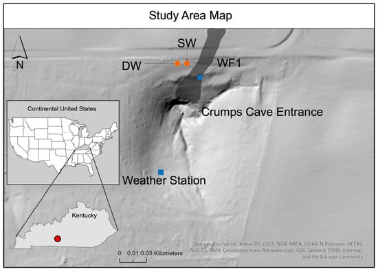
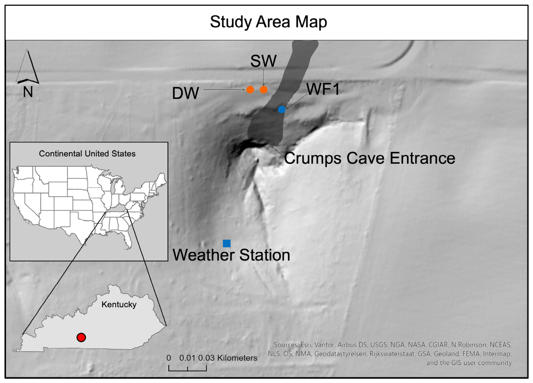
Crumps Cave, located in Smith’s Grove in northern Warren County, Kentucky (Figure 1), is part of the Pennyroyal Plateau sinkhole plain. The cave is owned by Western Kentucky University and encompasses several kilometers of mapped passages and multiple in-cave waterfalls located approximately 25 m below the surface. The entrance is part of a large one-hectare sinkhole with a nearly horizontal passage that measures on average 6 m tall and 18 m wide and is formed in upper St. Louis limestone with a roughly 2° dip to the northwest [18]. The surface vegetation surrounding the cave consists of deciduous trees and shrubs with diverse botanical flowering species and sub-tropic grasslands. The cave floor is about 25 m from the surface on which agriculture practices occur. Regional aquifer recharge lies within the Graham Springs groundwater basin and discharges at the Wilkins Blue Hole in the Barren River [19]. Water samples are collected as water drains through fractures and channels in the epikarst as a perennial waterfall (WF1) [20], which is located 40 m from the cave entrance and around 25 m below the surface, and is approximately 4.5 m in height, and at a shallow well (SW) at 15 m depth located above and adjacent to the cave and a deep well (DW) at 50 deep, located approximately 5 m apart. Both wells are 25.4 cm in diameter and cased to bedrock in the shallow soil.

Figure 1. Study area map of Crumps Cave in Warren County, Kentucky, U.S.A., with sampling locations of SW, DW, and WF1 indicated. Cave is in dark gray outline and not to scale. Red dot in Kentucky inset is study area location. Scale is for primary map, not insets.

An array of methodologies was used to collect, process, and analyze samples that originated from atmospheric and groundwater sources. Sampling occurred weekly between 30 September 2015, and 26 September 2017. A weather station south of the cave entrance was used to collect data on precipitation, relative humidity, and temperature. Agricultural production surrounds the cave and overlies the monitored waterfall, with various crop rotation through the seasons that primarily includes corn and soybean.

2.2. Field Sampling

Atmospheric GHG sample vials were prepared by using an evacuated 20 mL glass vial crimped with a gray butyl rubber septum. Samples were collected in triplicate from three different locations, at the surface, cave entrance, and near WF1, using a BD 60 mL syringe with a 23-gauge needle. The syringe was primed by filling and extracting three times to full capacity of the sampling air; thereafter, it was filled to 60 mL, where 35 mL was vented to the atmosphere and 25 mL was injected through the septum into the vial.

For the collection of dissolved GHGs, 9.5 mL of 0.1 N HCl was added to a 20 mL glass vial for each site in triplicate. Each vial was sealed using a gray butyl septum and placed on a built apparatus that would displace the air with ultra-high purity helium. At each sample site (DW, SW and WF1), a 0.5 mL of sample was injected through the septum using a 1 mL syringe with a 23-gauge needle into each vial and shaken to make a homogenous mixture [21].

On the surface, 1 L disposable well bailers (EcoBailer 78008, Forestry Suppliers, Jackson, MS, USA) were used to collect water samples from each well site, whereas grab samples were obtained from WF1. Water samples were transferred into a 500 mL Nalgene (Fisher Scientific, Pittsburgh, PA, USA), acid-washed, autoclaved bottle and placed into an ice-filled cooler. At each sample site, 100 mL of sample was used to clean and fill the reservoir of a YSI ProDSS (YSI Inc., Yellow Springs, OH, USA) water quality meter for determination of the water chemistry. The accuracy of the ProDSS is given according to the manufacturer for pH (±0.2 units), specific conductivity (SpC) (±0.001 uS∙cm⁻¹), temperature (±0.2 °C), and dissolved oxygen (DO) (±0.1 mg∙L⁻¹). Along with the water sampling at WF1, an EXO II data logger (YSI Inc., Yellow Springs, OH, USA) collected data every 10 min for pH (±0.2 units), specific conductivity (SpC) (±0.001 uS∙cm⁻¹), temperature (±0.2 °C), and dissolved oxygen (DO) (±0.1 mg∙L⁻¹), while pressure and temperature data within the discharge bucket located underneath the waterfall were collected every 10 min by a HOBO U-20 data logger (Onset Computer Corp, Bourne, MA, USA). All water samples were analyzed within a four-hour time frame of collection.

2.3. Meteorological Monitoring

Weather data were measured and recorded using a HOBO U-30 weather station (Onset Computer Corp., Bourne, MA, USA) on the surface of CC at a 10 min interval. Parameters monitored included temperature, relative humidity (RH), barometric pressure (BP), rainfall (mm/10 min), and wind speed. Inside the cave, near the entrance, a HOBO temperature/relative humidity datalogger collected data every ten minutes.

2.4. Sample Analysis

2.4.1. Greenhouse Gas Analysis

CO₂, N₂O, and CH₄ concentrations from aqueous samples were analyzed via headspace equilibration on a gas chromatograph (GC) (Varian CP-3800, Agilent Technologies, Santa Clara, CA, USA) that was modified to analyze greenhouse gases (RSC Group LLC, Katy, TX, USA). In total, 1 mL of vial headspace sample was injected by syringe and split by a switching valve, then transferred onto a 1.8 m × 1.6 cm column packed with 80/100 mesh Hay Sep Q (Varian Associates, Palo Alto, CA, USA) connected to a thermal conductivity detector (TCD) (Varian Associates, Palo Alto, CA, USA) that operated at 120 °C for CO₂ analysis. Another portion of the sample traveled from the TCD to a flame ionization detector (FID) (Varian Associates, Palo Alto, CA, USA) at 275 °C for CH₄ analysis. A third and final portion of the sample was split and transferred onto a 1.8 m × 1.6 cm Silicosteel column packed with 80/100 mesh Hay Sep Q (Varian Associates) connected to an electron capture detector (ECD) (Varian Associates, Palo Alto, CA, USA) that operated at 300 °C for N₂O analysis. Quantification was performed by calibration using standards of 1000, 5.0, and 2.0 µg L⁻¹ for CO₂, with an additional standard of 203,000 µg L⁻¹ included for CH₄ in N₂, and a two-point calibration for N₂O of 5.0 and 2.0 µg L⁻¹ in N₂ (Agilent Technologies, Santa Clara, CA, USA). Calibration standards were run every 30 samples and sample were all run in triplicate with the resulting data being the average of the three with Relative Standard Deviation (%RSD) ≤ 5% for all samples. Dissolved gas and bicarbonate concentrations were determined as previously described in [22], and all values are reported as dissolved gas in solution in units of mM/L (CO₂ and CH₄) or µM/L (N₂O), except for the cave atmospheric CO₂ data presented in ppmv.

2.4.2. Statistical Analysis

Data analysis was conducted across the dataset to derive means and standard deviations (SDs) for physicochemical data and medians and interquartile ranges (IQRs) for greenhouse gas (GHG) concentrations for each season and site. Two complementary statistical approaches were used to evaluate seasonal and site-level differences in dissolved CO₂ (mM), CH₄ (mM), and N₂O (µM) concentrations.

First, we tested for differences across the four individual seasons defined by common solstice and equinox periods: spring (21 March–20 June), summer (21 June–20 September), fall (21 September–20 December), and winter (21 December–20 March). Kruskal–Wallis H tests (df = 3) were applied separately to each site–gas combination (nine tests total). Effect size was quantified as η² = H/(N − 1), interpreted as: small ≥ 0.01, medium ≥ 0.06, large ≥ 0.14. Where the Kruskal–Wallis test was significant (α = 0.05), post hoc pairwise comparisons were conducted using the Mann–Whitney U test (two-sided) with Bonferroni correction across the six season pairs (α′ = 0.05/6 = 0.0083).

Second, to evaluate broader ecological patterns and improve statistical power, seasons were pooled into two groups: warm season (summer + fall) and cold season (winter + spring). Within each site–gas combination, warm and cold season concentrations were compared using Mann–Whitney U tests (two-sided, α = 0.05). Effect size for these comparisons was quantified using the rank-biserial correlation r, interpreted as: small ≥ 0.10, medium ≥ 0.30, large ≥ 0.50. To assess whether GHG concentrations differed between sites within each season group, Kruskal–Wallis H tests (df = 2) were applied across the three sites for each gas–season group combination. Where significant, pairwise site comparisons used Mann–Whitney U tests with Bonferroni correction across the three site pairs (α′ = 0.05/3 = 0.017). Effect size for site-level Kruskal–Wallis tests was again quantified as η² = H/(N − 1). All analyses were performed in Python v3.14.6, OriginPro v2024b, and SAS v15.4.

3. Results

3.1. Seasonal Physicochemical Variations

Annual rainfall was 1490.5 mm from 1 September 2015 to 30 September 2016 (15/16) and 1148.2 mm from 30 September 2016 to 1 October 2017 (16/17), with two major recorded rain events on 5 May 2016 and 12 May 2017. Discharge at WF1 was measured in liters per second (L s⁻¹) and baseflow was recorded at 0.013 L s⁻¹. The highest discharge level recorded was on 1 September 2017, at 11.319 L s⁻¹. This high discharge was due to Hurricane Harvey that produced 108.47 mm of precipitation within seven hours. The average discharge at WF1 for 2015–2016 and 2016–2017 was 0.042 and 0.036 L s⁻¹, respectively. Annual average cave air temperatures near WF1 remained mostly stable at 12.56 ± 2.01 °C during the study period.

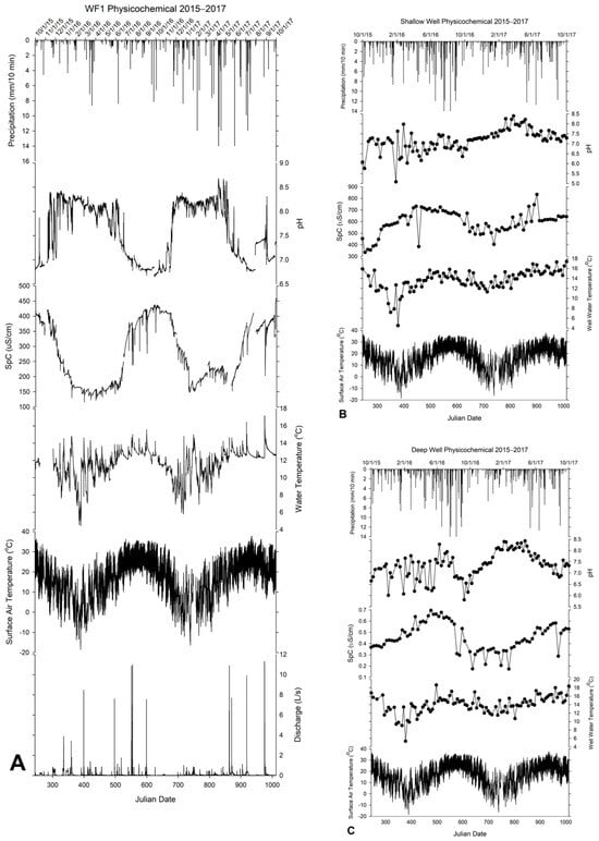
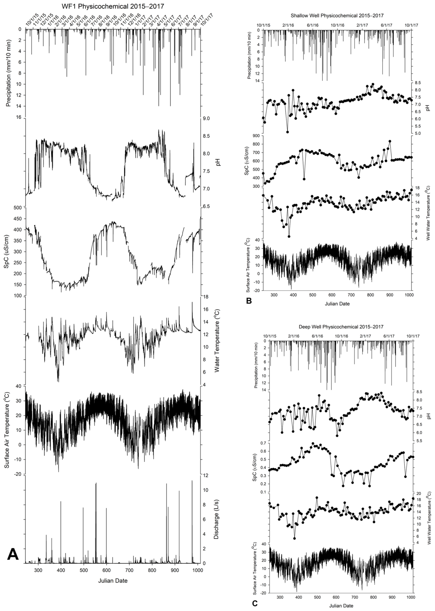
Hydrologic variations at SW and DW were measured as depth in meters, since it was not possible to measure discharge. Decreasing depth values indicate a rise in the water table. Base level at SW and DW was recorded during 2015–2017 when rainfall was at a minimum. SW had a base level of 16.28 m below the surface. At the highest level, SW peaked at 5.75 m below the surface on 24 November 2015. The rise occurred from a rain event that produced 27.14 mm two days prior. The average depth to the water table in SW was 14.58 m below the surface. SW is thought to be on a perched aquifer in the epikarst, approximately 15 m below the surface, that responds quickly to rain events. DW tends to follow the regional water table gradient and rise and fall in elevation similar to the Barren River, which flows around the City of Bowling Green, Kentucky, some 15 km to the south and reaches a base level depth of 41.23 m below the surface. The highest level of DW occurred on 20 December 2015, with a reading of 29.23 m when multiple rain events started on 25 October 2015, and ended on 28 December 2015, producing 50.66 mm of precipitation. Both SW and DW tend to lag in response to less extreme rain events compared to the faster flowpaths recharging WF1 per the discharge data (Figure 2).

Figure 2. Geochemistry of WF1, DW, and SW. (A) WF1 had a 10 min resolution sampling. Both (B) SW and (C) DW were sampled at weekly resolution.

The hydrogeochemical dynamics reflected in Table 1 give an indication of each sampling site as sampling progressed through each season. SW had the lowest recorded pH value (5.1) in the winter months and WF1 had the highest (8.9), which also occurred in the winter season. Waterfall and SW water temperatures during these extreme points were the coldest on average at 10.6 and 11.7 (°C), respectively.

Table 1. Average water physicochemistry from each sampling site pooled by season for the duration of the study.

	Average Physicochemical Parameter Values
	Temperature (°C)	Specific Conductivity (mS cm−1)	pH Average	pH Range	Turbidity (NTU)	Discharge (L s−1)
	Spring 2
WF1 1	12.1 ± 0.27	210 ± 40	7.7 ± 0.45	6.9–8.3	1.27 ± 15.80	0.09 ± 0.28
Shallow Well	14.8 ± 1.45	510 ± 10	7.3 ± 0.63	6.1–8.4	ND	ND
Deep Well	14.3 ± 1.74	370 ± 70	7.5 ± 0.66	6.2–8.4	ND	ND
	Summer 2
WF1 1	12.8 ± 0.65	380 ± 30	6.9 ± 0.22	6.7–8.3	0.27 ± 2.28	0.113 ± 0.58
Shallow Well	15.0 ± 1.02	630 ± 80	7.1 ± 0.32	6.4–7.7	ND	ND
Deep Well	15.4 ± 1.03	530 ± 80	7.1 ± 0.49	5.8–8.0	ND	ND
	Fall 3
WF1 1	10.6 ± 1.55	380 ±70	7.6 ± 0.61	6.7–8.4	−0.04 ± 0.761	0.07 ± 0.19
Shallow Well	13.3 ± 1.65	680 ± 20	7.0 ± 0.41	5.8–7.4	ND	ND
Deep Well	14.0 ± 1.93	560 ± 120	7.1 ± 0.36	6.0–7.7	ND	ND
	Winter 4
WF1 1	10.6 ± 1.95	180 ± 30	8.1 ± 0.12	5.9–8.9	0.19 ± 3.20	0.11 ± 0.022
Shallow Well	11.7 ± 2.31	540 ± 50	7.2 ± 0.76	5.1–8.3	ND	ND
Deep Well	12.1 ± 2.39	310 ± 60	7.6 ± 0.67	6.1–8.4	ND	ND

Note: NTU = Nephelometric Turbidity Units. ¹ 15 min resolution data represent the mean between 22,215 and 30,072 determinations ± standard deviation of the mean. ² Data represent the mean of 27 determinations. ³ Data represent the mean of 25 determinations. ⁴ Data represents the mean of 22 determinations ± standard deviation of the mean for both shallow and deep well only. ND = No data, as turbidity and discharge were not able to be measured for the wells.

At each site (WF1, DW, and SW), water temperature may have been a driving factor for geochemical SpC and pH changes, as shown in Figure 1. As the water temperature increases, movement of water molecules tends to be faster and can absorb more charged ions—indicating a rise in SpC [23]. Peak temperatures reached 17.1, 18.6, 17.4 °C at WF1, DW, and SW during the summer, spring, and fall, respectively (Figure 2). The corresponding pH values were 7.22, 7.45, and 7.29, respectively, for WF1, DW, and SW. SpC values peaked at 203, 431, and 643 µS cm⁻¹, respectively. Water temperatures decreased for WF1, DW, and SW to minimums of 4.4, 5.3, and 4.5 °C, respectively, and SpC values measured 163, 520 and 660 μS cm⁻¹, respectively, while pH measured 8.19, 6.85, and 6.22, all occurring in the winter months. Extreme fluctuations in temperature do not occur often in south-central Kentucky, due to mild winters and relatively low precipitation.

3.2. Dissolved Greenhouse Gases

Each site yielded 101 observations (n = 303 total), distributed across four meteorological seasons (spring, summer, fall, and winter) with 22–29 observations per site–season cell. Because gas concentration data are typically right-skewed, all central tendency and spread measures use medians and interquartile ranges (IQR = Q3 − Q1). Table 2 shows the median of the three GHGs at each sampling site for each season. Dissolved CO₂, CH₄, and N₂O vary seasonally due to dynamic factors such as weather, soil respiration, and anthropogenic processes. Water as a solvent entrains and transports more dissolved GHGs into and through the soil profile and epikarst into the groundwater, where they may later be emitted at remote sites. Seasonal medians and IQRs for each gas, site, and season are reported in Table 2, and statistical test results comparing seasons are summarized in Table 3. Pooled seasonal comparisons and site comparisons by season group are presented in Table 4 and Table 5.

Table 2. Seasonal dissolved greenhouse gas concentrations by site: medians, interquartile ranges, and Kruskal–Wallis test statistics (2015–2017).

		Spring		Summer		Fall		Winter		Kruskal–Wallis
Site	Gas	Median	IQR	Median	IQR	Median	IQR	Median	IQR	H	p-Value	η2
WF1	CO2 (mM/L)	1.60	0.76	4.59	1.42	3.35	3.62	1.42	0.55	62.31	<0.001	0.62
SW	CO2 (mM/L)	1.83	1.14	3.29	1.20	3.68	1.56	2.05	1.33	33.99	<0.001	0.34
DW	CO2 (mM/L)	2.26	0.66	4.21	1.42	4.87	3.56	2.01	0.96	55.8	<0.001	0.56
WF1	CH4 (mM/L)	0.02	0.02	0.03	0.07	0.03	0.02	0.03	0.03	5.43	0.143	0.05
SW	CH4 (mM/L)	0.03	0.04	0.21	0.31	0.50	1.62	0.13	1.34	19.73	<0.001	0.2
DW	CH4 (mM/L)	0.06	0.13	0.27	0.52	0.51	0.96	0.04	0.07	32.53	<0.001	0.33
WF1	N2O (µM/L)	2.64	9.80	1.36	4.05	0.85	2.66	5.74	35.29	10.46	0.015	0.1
SW	N2O (µM/L)	13.53	30.86	2.12	19.00	3.13	10.16	11.16	148.80	6.18	0.103	0.06
DW	N2O (µM/L)	5.24	10.92	0.77	7.50	2.18	3.36	7.34	51.81	9.19	0.027	0.09

Note: Medians pooled across 2015–2017 (n = 22–29 per site–season). IQR = Q3 − Q1. Kruskal–Wallis H test seasonal differences within each site–gas combination (df = 3); bold p-values indicate p < 0.05. η² = H/(N − 1); η² = size effect as small ≥ 0.01, medium ≥ 0.06, large ≥ 0.14.

Table 3. Pairwise seasonal comparisons: Mann–Whitney U p-values (Bonferroni-corrected, α′ = 0.0083) by site and GHG.

Site	Gas	Spr vs. Sum	Spr vs. Fal	Spr vs. Win	Sum vs. Fal	Sum vs. Win	Fal vs. Win
WF1	CO2 (mM/L)	<0.001 *	<0.001 *	0.020	0.097	<0.001 *	<0.001 *
SW	CO2 (mM/L)	<0.001 *	<0.001 *	0.608	0.253	<0.001 *	<0.001 *
DW	CO2 (mM/L)	<0.001 *	<0.001 *	0.066	0.701	<0.001 *	<0.001 *
WF1	CH4 (mM/L)	0.025	0.156	0.209	0.238	0.532	0.669
SW	CH4 (mM/L)	0.007 *	<0.001 *	0.017	0.015	0.937	0.174
DW	CH4 (mM/L)	<0.001 *	<0.001 *	0.165	0.062	<0.001 *	<0.001 *
WF1	N2O (µM/L)	0.231	0.241	0.084	0.768	0.007 *	0.004 *
SW	N2O (µM/L)	0.350	0.376	0.188	0.971	0.047	0.024
DW	N2O (µM/L)	0.145	0.350	0.175	0.341	0.006 *	0.020

Note: Two-sided Mann–Whitney U tests with Bonferroni correction (6 comparisons per site–gas; α′ = 0.0083). Bold values with * are statistically significant. Spr = spring, Sum = summer, Fal = fall, Win = winter.

Table 4. Greenhouse gas concentrations by grouped season (warm: summer + fall; cold: winter + spring) per site—Mann–Whitney U test results (2015–2017).

		Warm Season (Sum + Fall)			Cold Season (Win + Spr)			Mann–Whitney U
Site	Gas	Median	IQR	n	Median	IQR	n	U	p-Value	r
WF1	CO2 (mM/L)	4.30	2.86	52	1.49	0.59	49	2395	<0.001	−0.88
SW	CO2 (mM/L)	3.35	1.48	52	1.92	1.38	49	2123	<0.001	−0.67
DW	CO2 (mM/L)	4.41	2.46	52	2.22	1.02	49	2360	<0.001	−0.85
WF1	CH4 (mM/L)	0.03	0.03	52	0.02	0.03	49	1482	0.159	−0.16
SW	CH4 (mM/L)	0.30	0.73	52	0.05	0.33	49	1734	0.002	−0.36
DW	CH4 (mM/L)	0.43	0.49	52	0.05	0.13	49	2080	<0.001	−0.63
WF1	N2O (µM/L)	1.00	3.72	52	3.94	14.60	49	871	0.006	0.32
SW	N2O (µM/L)	2.63	13.18	52	12.24	33.38	49	964	0.035	0.24
DW	N2O (µM/L)	1.60	6.26	52	5.24	14.71	49	894	0.010	0.30

Note: Medians pooled across 2015–2017. IQR = Q3 − Q1. Mann–Whitney U test (two-sided); bold p-values significant at α = 0.05. r = rank-biserial correlation: small ≥ 0.10, medium ≥ 0.30, large ≥ 0.50. Positive r indicates cold > warm; negative r indicates warm > cold.

Table 5. Site comparisons within grouped seasons: medians, IQR, Kruskal–Wallis test, and Bonferroni-corrected pairwise site p-values (2015–2017).

		WF1		SW		DW		Kruskal–Wallis (Sites)			Pairwise Site p-Values
Season Group	Gas	Median	IQR	Median	IQR	Median	IQR	H	p-Value	η2	WF1 vs. SW	WF1 vs. DW	SW vs. DW
Warm (Sum + Fall)	CO2 (mM/L)	4.30	2.86	3.35	1.48	4.41	2.46	13.62	0.001	0.09	0.028	0.163	<0.001 *
Cold (Win + Spr)	CO2 (mM/L)	1.49	0.59	1.92	1.38	2.22	1.02	22.94	<0.001	0.16	0.001 *	<0.001 *	0.197
Warm (Sum + Fall)	CH4 (mM/L)	0.03	0.03	0.30	0.73	0.43	0.49	63.68	<0.001	0.41	<0.001 *	<0.001 *	0.300
Cold (Win + Spr)	CH4 (mM/L)	0.02	0.03	0.05	0.33	0.05	0.13	16.18	<0.001	0.11	<0.001 *	0.001 *	0.555
Warm (Sum + Fall)	N2O (µM/L)	1.00	3.72	2.63	13.18	1.60	6.26	5.66	0.059	0.04	0.020	0.326	0.150
Cold (Win + Spr)	N2O (µM/L)	3.94	14.60	12.24	33.38	5.24	14.71	4.09	0.129	0.03	0.061	0.392	0.169

Note: Medians pooled across 2015–2017. IQR = Q3 − Q1. Kruskal–Wallis H tests site differences within each season group (df = 2). η² = H/(N − 1); η² = size effect of small ≥ 0.01, medium ≥ 0.06, large ≥ 0.14. * Pairwise site comparisons use Mann–Whitney U with Bonferroni correction (3 pairs; α′ = 0.017); bold p-values (K-W) and those with * (Pairwise) are significant.

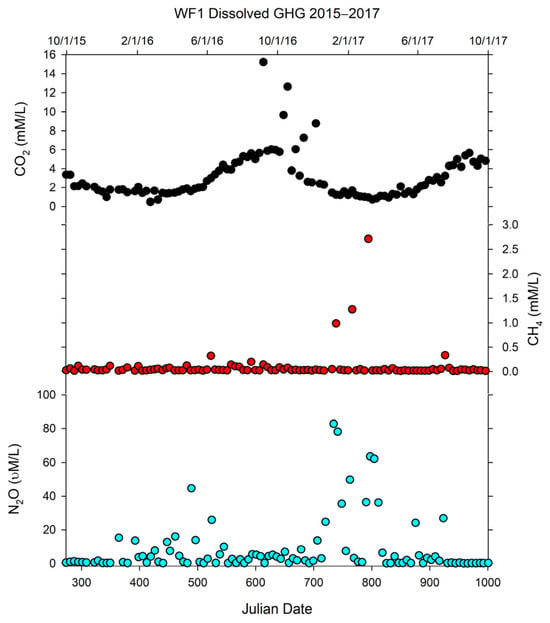
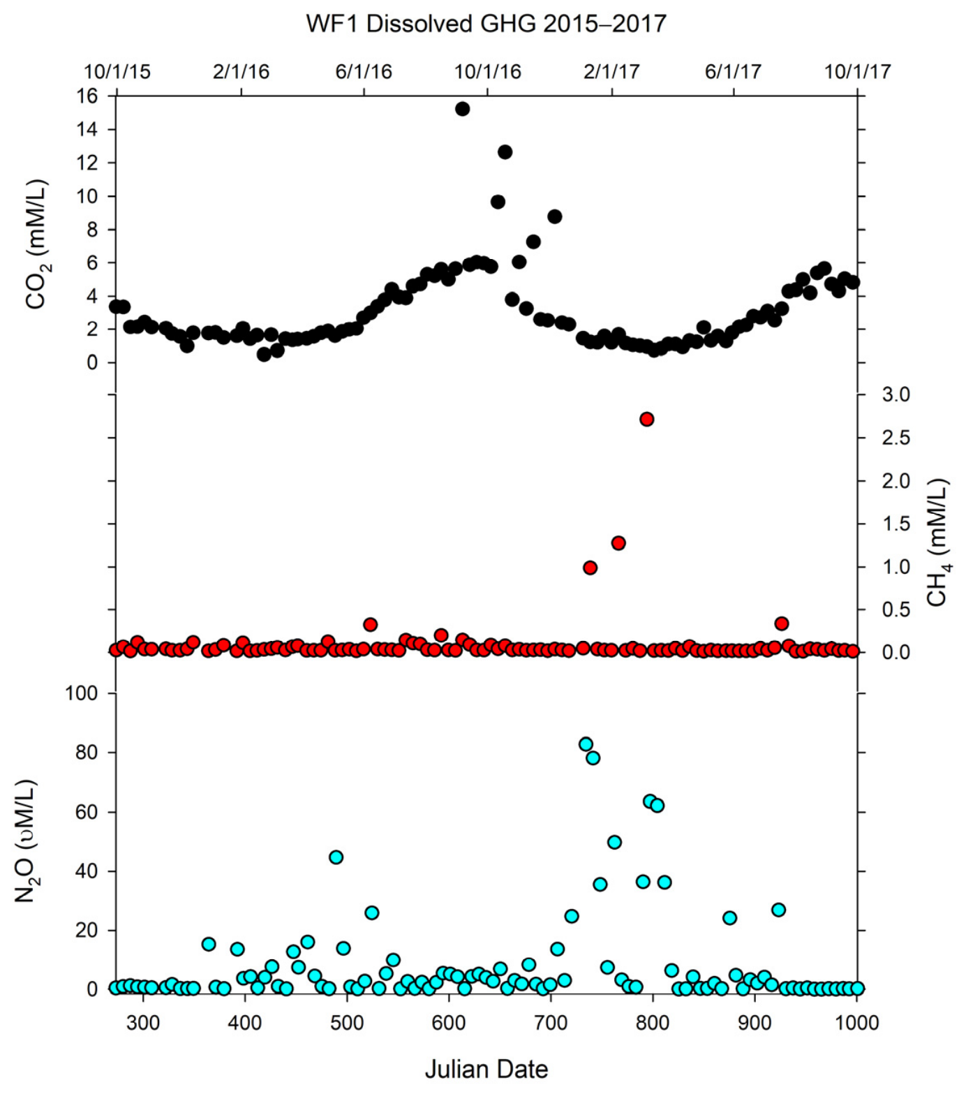
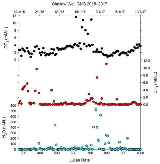
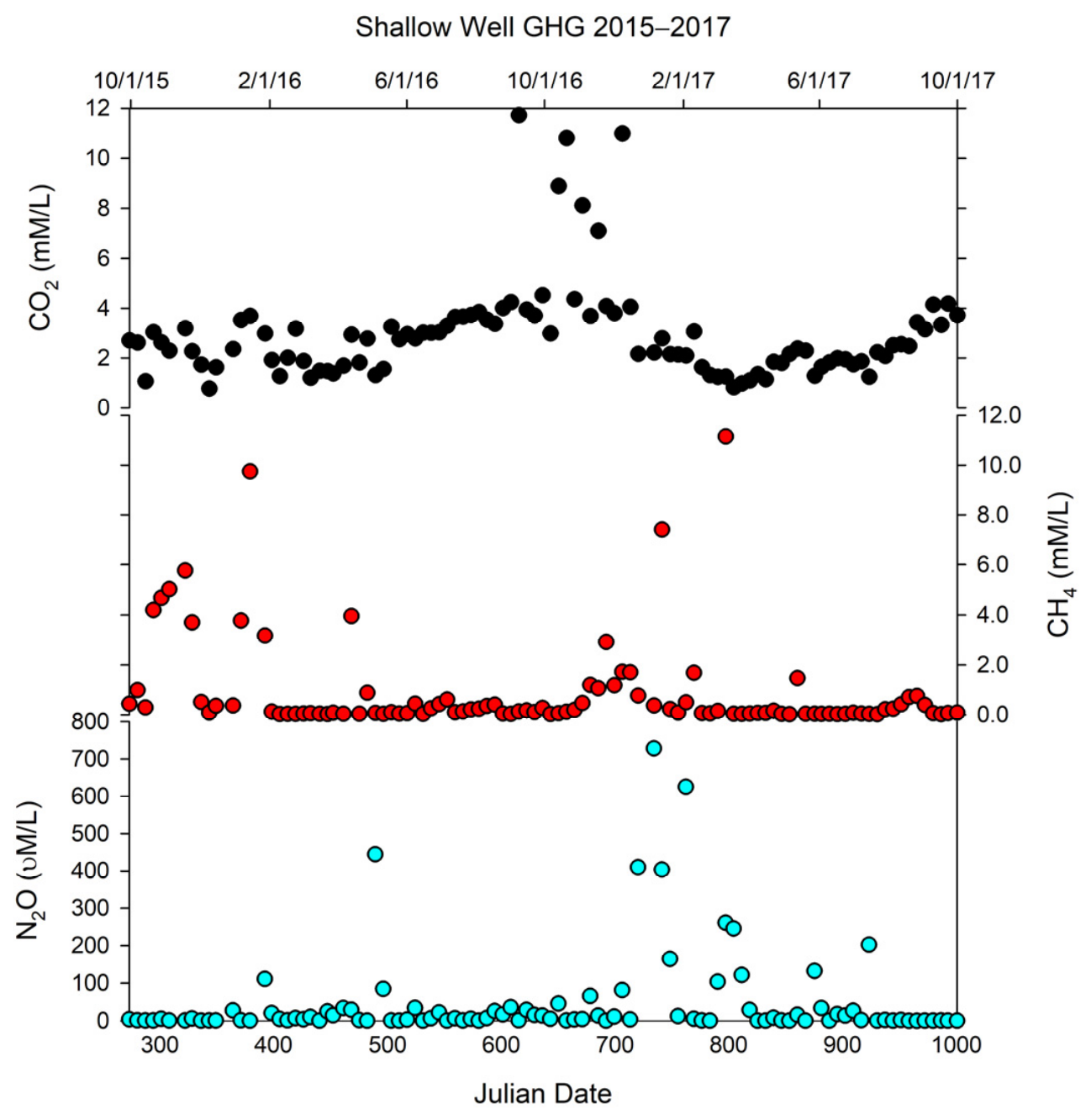
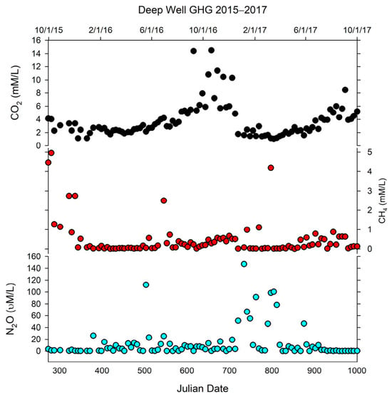
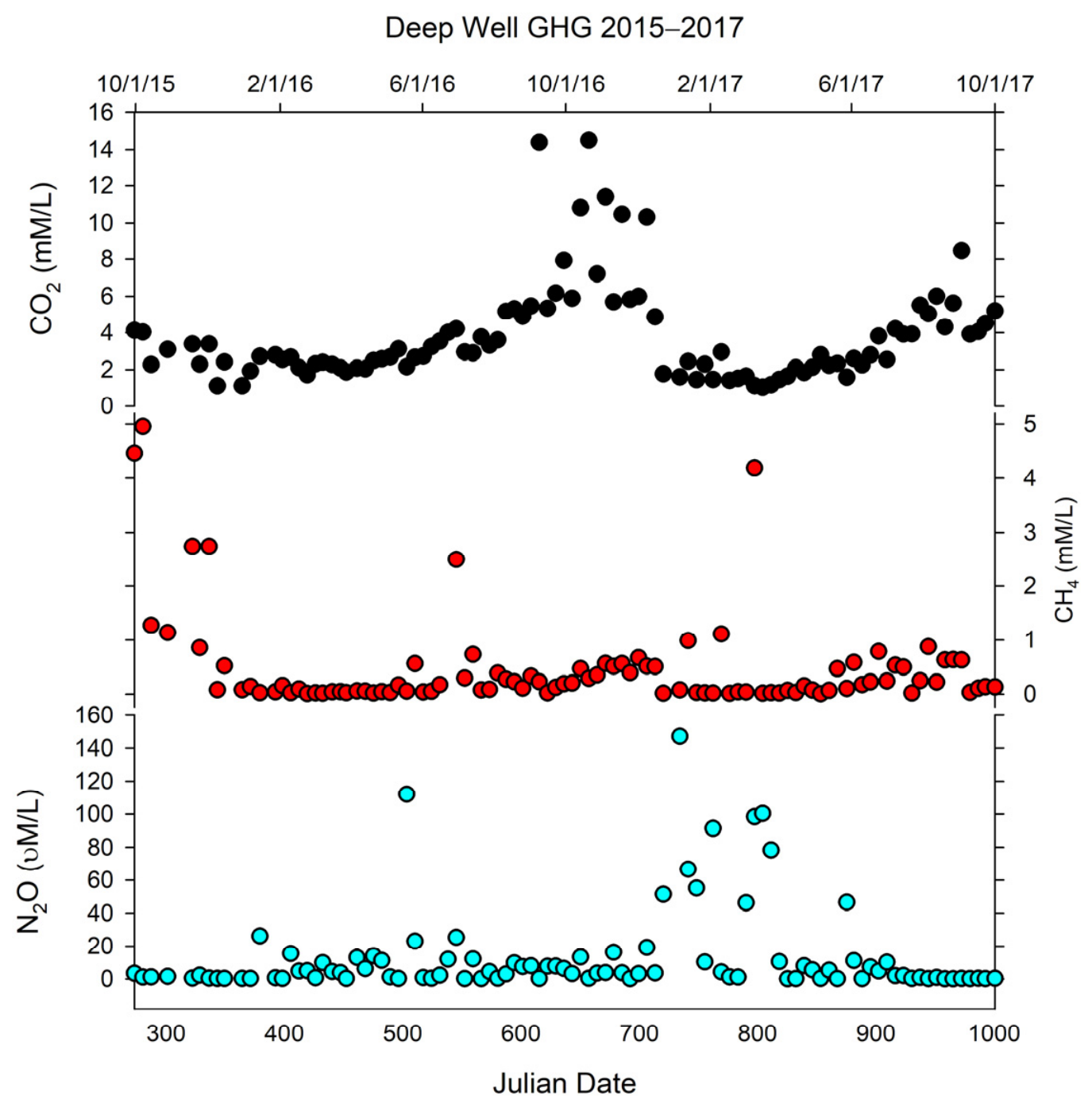
Table 2 and Figure 3, Figure 4 and Figure 5 indicate that the production of CO₂ increases in the warm season due to higher rates of soil respiration at all three sites (Kruskal–Wallis: WF1 H = 62.31, p < 0.001, η² = 0.62; SW H = 33.99, p < 0.001, η² = 0.34; DW H = 55.80, p < 0.001, η² = 0.56), with large effect sizes throughout (Table 2). Pairwise comparisons confirmed that summer and fall were each significantly higher than spring and winter at all sites (all p < 0.001 after Bonferroni correction), while summer and fall did not differ significantly from each other, nor did spring and winter (Table 3). When seasons were pooled, warm season (summer + fall) CO₂ was significantly higher than cold season (winter + spring) at all sites (all p < 0.001), with large effect sizes (rank-biserial r = −0.88 at WF1, −0.67 at SW, −0.85 at DW) (Table 4 and Table 5). At WF1, CO₂ may be stored in the epikarst or regional aquifer in dissolved form, causing higher concentrations and a longer infiltration period into the system during the summer and fall months. Because WF1 has more direct infiltration and rapid recharge, this would cause a more rapid change in CO₂ concentrations in response to warm seasons, when CO₂ accumulates in the epikarst due to root and biological activity. In Figure 3 and Figure 4, SW and DW have lag times where the seasonal increases in CO₂ are shifted later relative to WF1, due to the difference in depth and flowing water between WF1 and the two wells, which would take longer for dissolved CO₂ to reach via the groundwater system.

Figure 3. Dissolved greenhouse gas concentrations at Crumps Cave WF1.

Figure 4. Dissolved greenhouse gas concentrations at SW.

Figure 5. Dissolved greenhouse gas concentrations at DW.

CH₄ concentrations peak in the fall season across the sampling period, whereas N₂O concentrations were highest during the cooler months (winter/spring) (Figure 3, Figure 4 and Figure 5). Methane concentrations were significantly elevated in the warm season at SW and DW, but not at WF1, reflecting a site-dependent seasonal pattern (Figure 3, Figure 4 and Figure 5). Kruskal–Wallis tests were significant at SW (H = 19.73, p < 0.001, η² = 0.20) and DW (H = 32.53, p < 0.001, η² = 0.33), but not at WF1 (H = 5.43, p = 0.143, η² = 0.05), where concentrations remained uniformly low across all seasons (medians 0.02–0.03 mM). At SW and DW, CH₄ was highest in fall and summer and lowest in spring and winter. When seasons were pooled, warm season CH₄ was significantly higher than cold at SW (p = 0.002) and DW (p < 0.001), but not at WF1 (p = 0.159). Site comparisons confirmed that WF1 was significantly lower than both SW and DW in both warm (η² = 0.41) and cold season groups (all p < 0.001), while SW and DW did not differ significantly from each other in either season (Table 2, Table 3 and Table 4).

Nitrous oxide exhibited a seasonal pattern inverse to CO₂ and CH₄, with concentrations elevated in the cold season (winter + spring) and suppressed in the warm season (summer + fall) (Table 2, Table 3 and Table 4, Figure 3, Figure 4 and Figure 5). Kruskal–Wallis tests across the four individual seasons were significant at WF1 (H = 10.46, p = 0.015, η² = 0.10) and DW (H = 9.19, p = 0.027, η² = 0.09), and non-significant at SW (H = 6.18, p = 0.103, η² = 0.06) reflecting high intra-seasonal variability associated with episodic recharge events at that site (winter IQR = 148.80 µM). When seasons were pooled into warm and cold groups, cold season N₂O was significantly higher than warm at all three sites (WF1: p = 0.006, r = 0.32; SW: p = 0.035, r = 0.24; DW: p = 0.010, r = 0.30), with medium effect sizes throughout. Unlike CO₂ and CH₄, N₂O did not differ significantly between sites within either season group (warm: H = 5.66, p = 0.059; cold: H = 4.09, p = 0.129), indicating a consistent seasonal response across all sites regardless of their hydrological characteristics (Table 4 and Table 5).

3.3. Cave CO₂ Atmospheric Gas and Sampling Site Responses

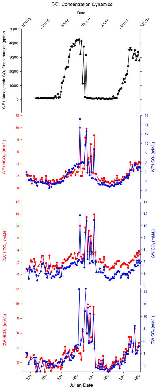
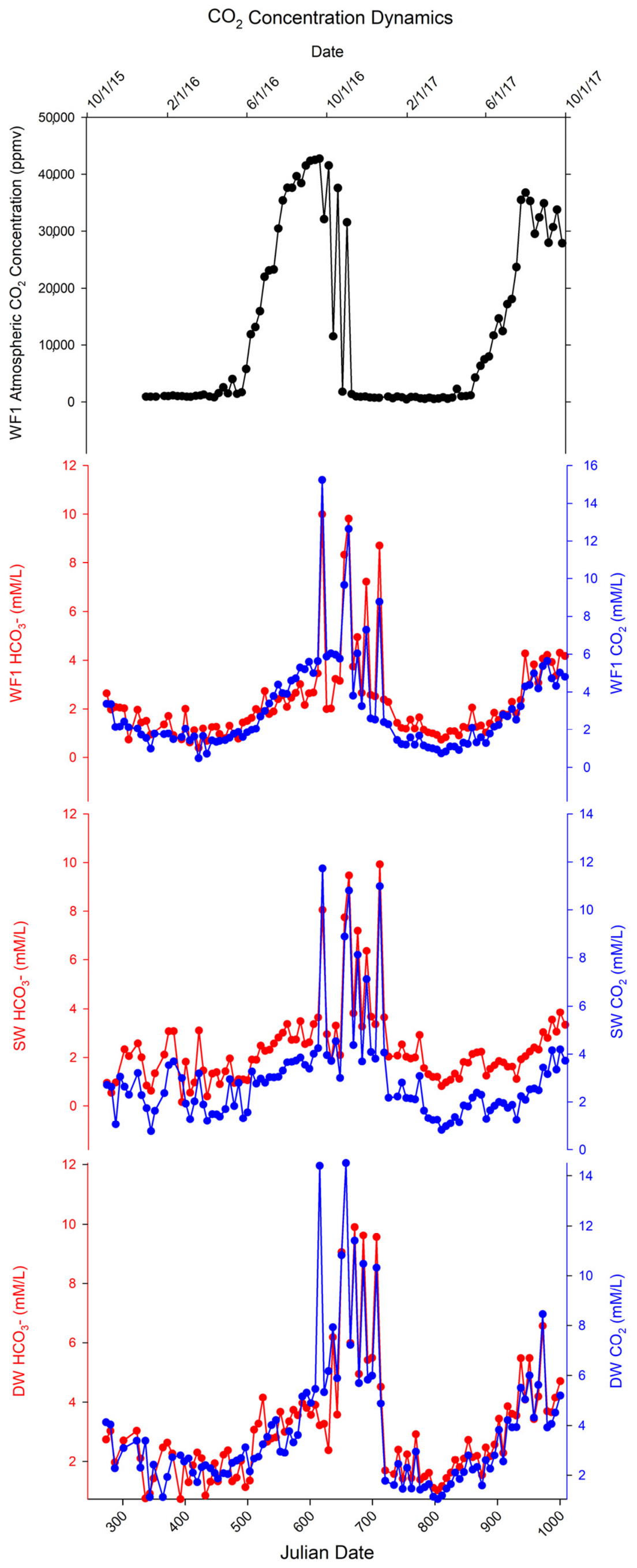
Cave atmospheric CO₂ (Figure 6) also followed a seasonal trend with the highest concentrations in the summer and fall, following the seasonal change in temperatures and vegetation activity. Root and microbial respiration increase dissolved CO₂ invading the groundwater system and creating carbonic acid, causing lower pH values during these months. This form of CO₂ is considered to influence cave formation [23,24,25]. Ref. [26] recently conducted a study on phreatic caves, which suggests that atmospheric CO₂ may help to accelerate cave genesis. Seasonal shifts reflect changes in cave atmosphere with respect to the growing season, which also influence CO₂ concentrations in the soil and epikarst [27]. Cave atmospheric carbon dioxide at WF1 was highest in the summer months at 42,800 ppmv and lowest in the winter at 422 ppmv. Table 3 presents the minimum/maximum concentrations of atmospheric CO₂, dissolved CO₂, and HCO₃- and the season when these extremes occurred. The seasonal trends indicate dissolution is actively occurring via carbonate dissolution primarily during the summer and fall periods when CO₂ concentration gradients are highest in the system. While the trends are similar between these datasets, the dissolved CO₂ values are more variable at each groundwater sampling site and more abrupt in response to changes in hydrologic drivers, while also being in a narrower range and lower concentrations than the cave air.

Figure 6. Cave atmospheric CO₂ at WF1 in conjunction with dissolved CO₂ and HCO³⁻ at WF1, SW, and DW. Notice the shift from WF1 to SW and DW. This is due to a “lag” time where the compounds must travel through the karst system and the effect of differing recharge rates. Seasonal effects on CO₂ exist across all sampling sites.

4. Discussion

4.1. Carbon Dioxide

Seasonal changes in pH at each sampling site are likely due to soil respiration from soil fauna, soil microorganisms and plant roots, all of which produce CO₂ in the soil zone that concentrates and may diffuse downward into the porous carbonate bedrock [24,25,26]. These factors represent seasonal differences that are either dormant or have slow respiration rates in cooler seasons and active respiration rates in warmer months, causing CO₂ concentration to fluctuate. Seasonal rain events generally transport CO₂ into the karst system, where it is transformed into carbonic acid which is mostly responsible for the dissolution of the limestone. The process slows down when temperatures decrease and reduces soil respiration.

Carbon dioxide at all three sites (Figure 2, Figure 3 and Figure 4) revealed concentrations and variability flow typical of a karst landscape [27,28]. This was confirmed statistically: Kruskal–Wallis tests showed highly significant seasonal variation in CO₂ at all three sites (WF1: H = 62.31, p < 0.001, η² = 0.62; SW: H = 33.99, p < 0.001, η² = 0.34; DW: H = 55.80, p < 0.001, η² = 0.56), with large effect sizes throughout (Table 2). Pairwise comparisons confirmed that summer and fall concentrations were each significantly higher than spring and winter at all three sites (all p < 0.001 after Bonferroni correction; Table 3), consistent with temperature-driven biological respiration during the growing season. During the growing season, increased soil temperatures encourage root growth and increase microbial activity in the soil, releasing respired CO₂ into the soil that can invade as dissolved CO₂ in the groundwater and lower its pH. This seasonal increase in soil CO₂ concentrations, and concomitant decrease in pH during the growing season, has been noted by previous researchers [29].

When seasons were pooled into warm (summer + fall) and cold (winter + spring) groups, the contrast remained highly significant at all sites (all p < 0.001), with large effect sizes (rank-biserial r = −0.88 at WF1, −0.67 at SW, −0.85 at DW; Table 3). The dissolved CO₂, along with carbonic acid and bicarbonate, transferred with the percolating waters moving through the epikarst and into the groundwater and caused a seasonal pH change. During the dry seasons of September to November, CO₂ was elevated in response to vegetation maturation at the surface which coincides with less precipitation, lower humidity, and lower soil moisture. As the seasons progress from warmer to cooler temperatures, soil microorganisms and root growth respond by decreasing respiration which may account for the limited CO₂ variation observed over the winter months [30]; however, bicarbonate concentration increased in the fall as pH increased and CO₂ values decreased in the winter (Table 1).

Carbon dioxide being produced and consumed may also be transported in groundwater through diffusion from high-concentration areas in the soil and epikarst. The deep well had more carbonate buffering as indicated by its specific conductivity values and bicarbonate values (Table 1). All three sites have different characteristics involving depth and lag time: SW and DW have slow recharge/discharge environments, while WF1 has a direct infiltration system where surface waters recharge directly and cause rapid changes in CO₂ concentrations. Site comparisons within season groups indicate that WF1 had significantly lower CO₂ than both SW and DW during the cold season (p = 0.001 and p < 0.001, respectively; Table 4), consistent with its direct epikarst infiltration characteristics. In both SW and DW, CO₂ can reversibly transform to bicarbonate where dissolution and deposition of bedrock occur. In the summer months, when pH is lower and CO₂ higher, latent CO₂ emissions seem more likely as groundwater moves downward at the sampling sites and causes a concentration gradient due to diffusion into the groundwater.

Carbon Dioxide Dynamics

Inorganic acids in the soil become more concentrated (due to higher rates of soil respiration) and rainfall transports dissolved CO₂ via rapid recharge through the soil and epikarst zones; hence, higher concentrations of carbonic acid enter the groundwater system where it dissolves the carbonate rock. As CO₂ moves into the groundwater, this may result in elevated CO₂ in the cave atmosphere, elevating it ten times or more compared to what is recorded at the surface [31], or may be released at the surface, redirecting back into the atmosphere. In the winter months, where the soil CO₂ produced at the surface is reduced due to microbial and/or root dormancy, cave atmospheric CO₂ may be diminished. Since the winter surface temperature may be lower than the average cave temperature (stable ~13 °C), the partial pressure is lower and the cave will vent out any accumulated CO₂. Ref. [32] recorded similar results in a show cave in Vietnam, where summer CO₂ concentrations recorded 13,500 ppmv compared to winter concentrations of 1500–3000 ppmv, which was explained by diminishing microbial activity and low surface temperatures. In this study, CO₂ concentrations in the cave were recorded exceeding 40,000 ppmv in September of 2016 and 30,000 ppmv in July–August 2017 (Figure 6). Dissolved CO₂ concentrations increased in water samples taken at WF1, SW, and DW during these periods. The spikes in the concentration of dissolved CO₂ were followed by increases in the concentration of HCO₃₋ suggesting resultant dissolution of carbonate minerals. There is a slight lag in the dissolved CO₂ response during the warm season transition, likely due to the slower buildup of CO₂ in the epikarst and vadose zones to create a gradient for downward migration into the groundwater system. These results suggest that karst groundwater in this region could be a large regional source of CO₂ emissions during the growing season, due to soil respiration, transport of CO₂ into the aquifer, and subsequent dissolution of carbonate minerals releasing CO₂ back to the environment. The magnitude of seasonal indirect CO₂ emissions would depend greatly upon the buffering capacity and pH of the receiving waters at the site of groundwater discharge (e.g., surface spring). Further studies would be needed to test this hypothesis and the magnitude of the potential emissions via this mechanism.

4.2. Methane

Since CH₄ is produced and consumed biologically, concentration peaks are likely driven by methanogenesis. Kruskal–Wallis tests revealed a significant site-dependent seasonal pattern: CH₄ varied significantly at SW (H = 19.73, p < 0.001, η² = 0.20) and DW (H = 32.53, p < 0.001, η² = 0.33), but not at WF1 (H = 5.43, p = 0.143, η² = 0.05; Table 2). The absence of a seasonal CH₄ signal at WF1, where concentrations remained uniformly low across all seasons (medians 0.02–0.03 mM), is consistent with its direct epikarst infiltration characteristics and predominantly oxic conditions, which suppress methanogenesis year-round. The low concentrations at WF1 may also reflect degassing and discharge occurring in the vadose zone. Soil tillage during the planting months of March–April may have caused concentration spikes as it releases organic matter (OM); however, OM availability and less dynamic recharge appear to be the principal drivers of CH₄ generation at SW and DW. CH₄ production in WFI was stable through the first year of the study (15–16) with a concentration peak of 0.32 mmol/L (Figure 3 and Figure 4), which occurred after a rain event on 5 June 2016, causing CH₄ to move through the epikarst and into the groundwater. The second year of the study (16–17) indicated a few spikes of CH₄ concentration (1.0 to 2.7 mmol/L) in late spring (Figure 3 and Figure 4), also occurring around rain events.

At SW and DW, CH₄ was markedly elevated in summer and fall and lowest in spring and winter, consistent with the fall and winter months providing decaying OM as a source for methanogenesis [33]. Pairwise tests confirmed these contrasts: at DW, spring values were significantly lower than summer and fall values, and winter values were significantly lower than summer and fall values (all p < 0.001; Table 2). Grouping seasons confirmed this pattern: warm season CH₄ was significantly higher than cold at SW (p = 0.002, r = −0.36) and DW (p < 0.001, r = −0.63), but not at WF1 (p = 0.159; Table 3). The erratic CH₄ concentrations observed at SW and DW during fall and winter, when OM from vegetation, arthropods, and seasonal biota is decaying and transported via precipitation, contrast with the minimal concentration differences during spring and summer, probably due to reduced rainfall and lower availability of organic carbon at the time. Ref. [1] also found an increase in CH₄ in the fall season due to OM decaying.

Importantly, WF1 was significantly lower than both SW and DW in both warm (p < 0.001, η² = 0.41) and cold seasons (p < 0.001 and p = 0.001, respectively; Table 4), while SW and DW did not differ from each other in either season group. This indicates that hydrological connectivity and anaerobic conditions, rather than specific site characteristics, are likely the key drivers of CH₄ production, with WF1’s variable flow and more oxic conditions suppressing methanogenesis that SW and DW sustain year-round through their slower recharge/discharge dynamics.

4.3. Nitrous Oxide

Nitrous oxide is significantly influenced by anthropogenic land use [34]. Ultimately, N₂O at all three sampling sites was driven by land use through fertilizer application and rainfall recharge events that supply the nitrogen source needed for the nitrogen cycle. Anhydrous ammonia was applied to the field adjacent to the site prior to planting corn in the spring. Winter wheat was planted in the fall, and soybeans which fix N and require no N fertilization were planted following the wheat harvest in mid-summer, reducing inorganic nitrogen accumulation during that period. The timing of when the N source enters the ground influences its residence time in the epikarst and potential concentration for availability in microbiological processes. Rapid recharge in the epikarst reduces the time available for nitrifiers and denitrifiers to utilize and reduce nitrates derived from surface fertilizer applications [35], and rapid discharge at WF1 may prevent denitrifiers from reducing NO₃⁻ to NO₂⁻. When water levels were low at SW and DW, indicating slower groundwater movement and less recharge, N₂O concentrations were low, consistent with denitrification proceeding more completely under extended residence times. Recharge flushes the NO₃⁻ into the groundwater, leaving an insufficient N source for the first stage of the nitrogen cycle to occur. This may affect other microbial populations in the denitrification process by reducing the population as a whole because of reduced soil moisture or oxygenated soil conditions [36]. Water levels were measured at SW and DW, since discharge could not be measured, and used as proxies for groundwater movement in the bedrock. When the water level was low, the well water was moving slower and receiving less recharge, allowing time for denitrification as evidenced by the low concentrations of N₂O (Figure 3) during late June through January, when rainfall was less (Figure 1, precipitation) in 2016 and 2017. Conversely, N₂O concentrations were higher at all three sample sites (WF1, SW, and DW) between February and June of 2016 and 2017. Aboveground agricultural practices where soil may be disturbed and applied fertilizers may increase soil nitrogen levels that would become mobile and able to enter the groundwater system.

Statistically, N₂O showed a seasonal pattern inverse to CO₂ and CH₄: concentrations were elevated in cold seasons (winter + spring) and suppressed in warm seasons at all three sites. Kruskal–Wallis tests across the four individual seasons were significant at WF1 (H = 10.46, p = 0.015, η² = 0.10) and DW (H = 9.19, p = 0.027, η² = 0.09), and marginally non-significant at SW (H = 6.18, p = 0.103, η² = 0.06; Table 1). At SW, winter and spring medians were notably elevated (11.16 and 13.53 µM, respectively) compared to summer (2.12 µM) and fall (3.13 µM); yet, no pairwise contrast survived Bonferroni correction due to extreme variability, as winter IQR at SW was 148.80 µM with individual observations reaching 728 µM (Table 2), likely reflecting episodic high-N₂O pulse events associated with freeze–thaw cycles or intermittent fertilizer loading. N₂O concentrations were higher at all three sites between February and June of 2016 and 2017, coinciding with aboveground agricultural practices, soil disturbance, and fertilizer application.

When seasons were pooled into warm and cold groups, the N₂O signal became clearer. Cold season concentrations were significantly higher than warm at all three sites, WF1 (p = 0.006, r = 0.32), SW (p = 0.035, r = 0.24), and DW (p = 0.010, r = 0.30; Table 3), with medium effect sizes throughout. This is consistent with cold-season denitrification dynamics: lower temperatures slow N₂O reductase activity relative to overall denitrification, leading to N₂O accumulation in winter and spring rather than complete reduction to N₂ [36]. Critically, N₂O concentrations did not differ significantly between sites within either season group (warm: H = 5.66, p = 0.059; cold: H = 4.09, p = 0.129; Table 4), indicating that seasonal, temperature-driven denitrification, rather than site-specific hydrology, governs N₂O dynamics across this system. This contrasts with CH₄, where site hydrology was the dominant control, and CO₂, where seasonal and site effects both contributed.

4.4. Impacts on Indirect Dissolved GHGs

The epikarst can store varying volumes of water on a local scale compared to primary aquifers that hold large volumes of water and supply large regions [28,37]; thus, karst groundwater systems may be a source of indirect GHG emissions under agricultural land use. The statistical analyses presented here support and extend this view, as each gas is governed by a distinct combination of seasonal and site-level controls, with CO₂ driven predominantly by temperature and seasonal respiration, CH₄ by site hydrology and anaerobic conditions, and N₂O by seasonal temperature effects on denitrification that are broadly consistent across all three sites regardless of hydrological characteristics. As stated by [3,38], the dynamics of indirect GHGs need more research to identify sources and sinks along with temporal evolution of karst systems under varying storm conditions and soil saturation and GHG production rates that are affected by land use. Nitrous oxide in particular requires further investigation to understand how soil biota, through the N cycle, affect GHG concentrations [39], especially given the episodic high-concentration pulse events observed at SW. By examining how NO₃⁻ is transformed through nitrification and denitrification, and the use of isotope tracers, a better understanding of which sources of N are being used, either organic or inorganic, can be gleaned. Organic N may stay in the soil longer due to mineralization, resulting in less N leachate transported into the groundwater system. New studies exploring the dynamics of dissolved inorganic carbon and OM may help to reveal how CH₄ is transported through the epikarst and into groundwater even in very deep aquifers.

5. Conclusions

Dissolved CO₂, N₂O, and CH₄ varied markedly across seasons at all three sampling sites, driven by a combination of agricultural practices, precipitation, soil biological activity, and site hydrology. Statistical analysis confirmed that each gas is governed by a distinct set of controls, with seasonal patterns and site-level differences that are ecologically interpretable and statistically robust. The fate of each GHG is determined by how it was formed and transported within the karst system.

Carbon dioxide showed the strongest and most consistent seasonal signal of the three gases, with significantly higher concentrations in warm seasons (summer + fall) than cold seasons (winter + spring) at all three sites (all p < 0.001, η² = 0.34–0.62). This pattern reflects temperature-driven soil respiration: microbial and root activity during the growing season elevates dissolved CO₂ in the soil zone, which is transported by rainfall into the karst system where it forms carbonic acid, lowers groundwater pH, and drives dissolution of carbonate bedrock. As a seasonal shift occurs from summer to winter, CO₂ production declines, pH rises, and bicarbonate concentrations increase [1,40,41,42,43]. Groundwater serves as the medium that entrains and transports each individual gas within the groundwater system, and the three sites differ in the rate at which this occurs: WF1, with its direct infiltration system, responds rapidly to surface CO₂ inputs, while the slower recharge environments of SW and DW buffer and delay the signal. These dynamics suggest that karst groundwater in this region may be a significant regional source of CO₂ emissions during the growing season, warranting further quantification.

Higher concentrations of dissolved N₂O seemed to be a result of fertilizer application whether in organic or inorganic form [1]. Since N₂O is a by-product of denitrification, its concentration is influenced by BMPs directly linked to land use [36]. Nitrous oxide exhibited a seasonal pattern inverse to CO₂ and CH₄: concentrations were significantly elevated in cold seasons (winter + spring) relative to warm seasons at all three sites (WF1: p = 0.006; SW: p = 0.035; DW: p = 0.010), consistent with cold-season denitrification dynamics in which lower temperatures slow N₂O reductase activity and lead to N₂O accumulation rather than complete reduction to N₂. Critically, N₂O did not differ significantly between sites in either season group, indicating that temperature-driven denitrification, rather than site hydrology, is the primary control. This site-independent response reflects the influence of surface agricultural practices and fairly consistent karst groundwater temperatures. Fertilizer application in spring and the nitrogen cycle processes that follow are broadly expressed across all three sites regardless of their hydrological characteristics. Residual nitrates leaching through the epikarst and bedrock accumulate in groundwater and may be redirected into streams and rivers, representing a diffuse nitrogen loss pathway linked directly to land use.

Methane concentrations were governed primarily by site hydrology rather than season alone. At WF1, CH₄ remained uniformly low year-round (medians 0.02–0.03 mM), consistent with the oxic conditions of a direct-infiltration upland site that suppress methanogenesis regardless of season. At SW and DW, CH₄ was significantly elevated in warm seasons relative to cold (p < 0.001 and p = 0.002, respectively), likely driven by the availability of decaying organic matter, particularly in fall and winter, and the anaerobic conditions sustained by slower groundwater recharge [44]. WF1 was statistically distinguishable from both SW and DW in both season groups (η² = 0.41 in warm seasons), while SW and DW did not differ from each other, suggesting that hydrological connectivity and persistent anoxia are the primary prerequisites for methane production in this karst system.

Collectively, these findings demonstrate that indirect greenhouse gas dynamics in karst groundwater under agricultural land use are gas-specific, seasonally structured, and mediated by the interplay of microbial activity, site hydrology, and land management. CO₂ and CH₄ are shaped by both season and site character, while N₂O is driven primarily by seasonal temperature and agricultural nitrogen inputs uniformly across sites. Indirect greenhouse gases are linked to karst groundwater systems and can be transported from, or stored within, the vadose and epiphreatic zones of karst aquifers under agricultural lands. Best management practices in karst agricultural areas, including timing of fertilizer application, tillage practices, and management of organic matter inputs, may influence indirect GHG concentrations through complex interactions of groundwater recharge, microbial activity, and seasonal land-use variability. Further quantification of both the transport and fate of indirect GHGs in karst systems may provide additional data to supplement GHG cycle modeling and inform air quality remediation strategies in rural karst areas where agricultural practices prevail.

References

- Sawamoto, T.; Kusa, K.; Hu, R.; Hatano, R. Dissolved N2O, CH4, and CO2 emissions from subsurface-drainage in a structured clay soil cultivated with onion in Central Hokkaido, Japan. Soil Sci. Plant Nutr. 2003, 49, 31–38. [Google Scholar]
- Jahangir, M.; Johnston, P.; Khalil, M.; Hennessy, D.; Humphreys, J.; Fenton, O.; Richards, K. Groundwater: A pathway for terrestrial C and N losses and indirect greenhouse gas emissions. Agric. Ecosyst. Environ. 2012, 159, 40–48. [Google Scholar] [CrossRef] [Scilit]
- Jurado, A.; Borges, A.V.; Pujades, E.; Hakoun, V.; Otten, J.; Knöller, K.; Brouyère, S. Occurrence of greenhouse gases in the aquifers of the Walloon Region (Belgium). Sci. Total Environ. 2018, 619, 1579–1588. [Google Scholar] [CrossRef] [Scilit] [PubMed]
- National Oceanic and Atmospheric Administration. Greenhouse Gases. 2016. Available online: https://gml.noaa.gov/ccgg/ (accessed on 20 May 2025).
- Environmental Protection Agency. Agriculture Sector Emissions. 2025. Available online: https://www.epa.gov/ghgemissions/agriculture-sector-emissions (accessed on 4 April 2025).
- Kasimir-Klemedtsson, A.; Klemedtsson, L.; Berglund, K.; Martikainen, P.; Silvola, J.; Oenema, O. Greenhouse gas emissions from farmed organic soils: A review. Soil Use Manag. 1997, 13, 245–250. [Google Scholar] [CrossRef] [Scilit]
- Bouwman, A.F. Direct emission of nitrous oxide from agricultural soils. Nutr. Cycl. Agroecosystems 1996, 46, 53–70. [Google Scholar] [CrossRef] [Scilit]
- Laini, A.; Bartoli, M.; Castaldi, S.; Viaroli, P.; Capri, E.; Trevisan, M. Greenhouse gases (CO2, CH4 and N2O) in lowland springs within an agricultural impacted watershed (Po River Plain, northern Italy). Chem. Ecol. 2011, 27, 177–187. [Google Scholar]
- Smith, P.; Martino, D.; Cai, Z.; Gwary, D.; Janzen, H.; Kumar, P.; McCarl, B.; Ogle, S.; O’Mara, F.; Rice, C.; et al. Greenhouse gas mitigation in agriculture. Philos. Trans. R. Soc. B Biol. Sci. 2008, 363, 789–813. [Google Scholar]
- Snyder, C.; Bruulsema, T.; Jensen, T.; Fixen, P. Review of greenhouse gas emissions from crop production systems and fertilizer management effects. Agric. Ecosyst. Environ. 2009, 133, 247–266. [Google Scholar] [CrossRef] [Scilit]
- Roberts, T. Right product, right rate, right time and right place… the foundation of best management practices for fertilizer. Fertil. Best Manag. Pract. 2007, 29, 1–8. [Google Scholar]
- Fixen, P. Can we define a global framework within which fertilizer best management practices can be adapted to local conditions? Fertil. Best Manag. Pract. 2007, 77. [Google Scholar]
- Snyder, C.S. Fertilizer Nitrogen BMPs to Limit Losses that Contribute to Global Warming. Fertilizer Best Management Practices. Norcross, Georgia, USA: International Plant Nutrition Institute; 2008, Ref. # 08057, Item 30-3210. Available online: http://npg.ipni.net/article/NPG-3005 (accessed on 4 April 2025).
- Reay, D.S.; Edwards, A.C.; Smith, K.A. Importance of indirect nitrous oxide emissions at the field, farm and catchment scale. Agric. Ecosyst. Environ. 2009, 133, 163–169. [Google Scholar] [CrossRef] [Scilit]
- Minamikawa, K.; Nishimura, S.; Sawamoto, T.; Nakajima, Y.; Yagi, K. Annual emissions of dissolved CO2, CH4, and N2O in the subsurface drainage from three cropping systems. Glob. Change Biol. 2010, 16, 796–809. [Google Scholar] [CrossRef] [Scilit]
- Madonia, P.; Bellanca, A.; Di Pietro, R.; Mirabello, L. The role of near-surface cavities in the carbon dioxide cycle of karst areas: Evidence from the Carburangeli Cave Natural Reserve (Italy). Environ. Earth Sci. 2012, 67, 2423–2439. [Google Scholar] [CrossRef] [Scilit]
- Madonia, P.; Cangemi, M.; Casamento, G.; Di Maggio, C.; Di Pietro, R.; Interlandi, M.; Barraco, G.; D’aleo, R.; Di Trapani, F. Atmospheric CO2 concentrations in caves protected as nature reserves and related gas hazard. Atmosphere 2022, 13, 1760. [Google Scholar] [CrossRef] [Scilit]
- Wang, J.; Li, L.; Liu, Y.; Li, W. A review of partial nitrification in biological nitrogen removal processes: From development to application. Biodegradation 2021, 32, 229–249. [Google Scholar] [CrossRef] [Scilit] [PubMed]
- Fierer, N. Embracing the unknown: Disentangling the complexities of the soil microbiome. Nat. Rev. Microbiol. 2017, 15, 579–590. [Google Scholar] [CrossRef] [Scilit] [PubMed]
- Groves, C.; Polk, J.S.; Miller, B.; Kambesis, P.; Bolster, C.; Vanderhoff, S.; Tyrie, B.; Ruth, M.; Ouellette, G.; Osterhoudt, L.; et al. The Western Kentucky University Crumps Cave Research and Education Preserve. In Proceedings of the 20th National Cave and Karst Management Symposium (NCKMS 3); National Cave and Karst Research Institute (NCKRI): Carlsbad, NM, USA, 2013. [Google Scholar]
- Polk, J.S.; Vanderhoff, S.; Groves, C.; Miller, B.; Bolster, C.; Thomas, S.A.; Meiman, J.; May, W.; Ruth, M.; Ouellette, G.; et al. Multiple Storm Event Impacts on Epikarst Storage and Transport of Organic Soil Amendments in South-central Kentucky. In Proceedings of the 20th National Cave and Karst Management Symposium (NCKMS 2013); National Cave and Karst Research Institute (NCKRI): Carlsbad, NM, USA, 2013. [Google Scholar]
- Loughrin, J.H.; Antle, S.W.; Polk, J. A gas chromatographic method for the determination of bicarbonate and dissolved gases. Front. Environ. Sci. 2017, 5, 65. [Google Scholar] [CrossRef] [Scilit]
- Groves, C.; Bolster, C.; Meiman, J. Spatial and temporal variations in epikarst storage and flow in south central Kentucky’s Pennyroyal Plateau sinkhole plain. In Proceedings of the U.S. Geological Survey Karst Interest Group Proceedings, Rapid City, SD, USA, 12–15 September 2005; pp. 64–73. [Google Scholar]
- Stroup, W.W.; Milliken, G.A.; Claassen, E.A.; Wolfinger, R.D. SAS for Mixed Models: Introduction and Basic Applications; SAS Institute: Cary, NC, USA, 2018. [Google Scholar]
- Cao, M.; Lei, J.; He, Q.; Zeng, Z.; Lü, X.; Jiang, Y. Rainfall-driven and hydrologically-controlled variations in cave CO2 sources and dynamics: Evidence from monitoring soil CO2, stream flow and cave CO2. J. Hydrol. 2021, 595, 126060. [Google Scholar] [CrossRef] [Scilit]
- Gulley, J.; Martin, J.; Moore, P.J.; Murphy, J. Formation of phreatic caves in an eogenetic karst aquifer by CO2 enrichment at lower water tables and subsequent flooding by sea level rise. Earth Surf. Process. Landf. 2013, 38, 1210–1224. [Google Scholar]
- Gulley, J.D.; Martin, J.B.; Moore, P.J.; Brown, A.; Spellman, P.D.; Ezell, J. Heterogeneous distributions of CO2 may be more important for dissolution and karstification in coastal eogenetic limestone than mixing dissolution. Earth Surf. Process. Landf. 2015, 40, 1057–1071. [Google Scholar] [CrossRef] [Scilit]
- Liu, Z.; Dreybrodt, W.; Wang, H. A new direction in effective accounting for the atmospheric CO2 budget: Considering the combined action of carbonate dissolution, the global water cycle and photosynthetic uptake of DIC by aquatic organisms. Earth-Sci. Rev. 2010, 99, 162–172. [Google Scholar] [CrossRef] [Scilit]
- Yang, R.; Liu, Z.; Zeng, C.; Zhao, M. Response of epikarst hydrochemical changes to soil CO2 and weather conditions at Chenqi, Puding, SW China. J. Hydrol. 2012, 468, 151–158. [Google Scholar] [CrossRef] [Scilit]
- White, W.B. Geomorphology and Hydrology of Karst Terrains; Oxford University Press: New York, NY, USA, 1988. [Google Scholar]
- Jackson, L.; Polk, J.S. Seasonal δ13CDIC sourcing and geochemical flux in telogenetic epikarst of south-central Kentucky. Earth Surf. Process. Landf. 2020, 45, 785–799. [Google Scholar] [CrossRef] [Scilit]
- Thompson, T.K.; Mclaughlin, D.L.; Schreiber, M.E.; Stewart, R.D. Assessing Landscape and Seasonal Controls on Soil CO2 Fluxes in a Karst Sinkhole. Environ. Eng. Geosci. 2023, 29, 217–229. [Google Scholar] [CrossRef] [Scilit]
- Doctor, D.H.; Kendall, C.; Sebestyen, S.D.; Shanley, J.B.; Ohte, N.; Boyer, E.W. Carbon isotope fractionation of dissolved inorganic carbon (DIC) due to outgassing of carbon dioxide from a headwater stream. Hydrol. Process. Int. J. 2008, 22, 2410–2423. [Google Scholar]
- Ek, C.; Gewelt, M. Carbon dioxide in cave atmospheres. New results in Belgium and comparison with some other countries. Earth Surf. Process. Landf. 1985, 10, 173–187. [Google Scholar] [CrossRef] [Scilit]
- Trinh, D.A.; Trinh, Q.H.; Tran, N.; Guinea, J.G.; Mattey, D. Eco-friendly remediation of lampenflora on speleothems in tropical karst caves. J. Cave Karst Stud. 2018, 80, 1–12. [Google Scholar] [CrossRef] [Scilit]
- Kotsyurbenko, O.; Nozhevnikova, A.; Zavarzin, G. Methanogenic degradation of organic matter by anaerobic bacteria at low temperature. Chemosphere 1993, 27, 1745–1761. [Google Scholar] [CrossRef] [Scilit]
- Lam, S.K.; Suter, H.; Bai, M.; Walker, C.; Davies, R.; Mosier, A.R.; Chen, D. Using urease and nitrification inhibitors to decrease ammonia and nitrous oxide emissions and improve productivity in a subtropical pasture. Sci. Total Environ. 2018, 644, 1531–1535. [Google Scholar] [CrossRef] [Scilit] [PubMed]
- Visser, A.-N.; Lehmann, M.F.; Rügner, H.; D’aFfonseca, F.M.; Grathwohl, P.; Blackwell, N.; Kappler, A.; Osenbrück, K. Fate of nitrate during groundwater recharge in a fractured karst aquifer in Southwest Germany. Hydrogeol. J. 2021, 29, 1153–1171. [Google Scholar] [CrossRef] [Scilit]
- Jahangir, M.; Johnston, P.; Barrett, M.; Khalil, M.; Groffman, P.; Boeckx, P.; Fenton, O.; Murphy, J.; Richards, K. Denitrification and indirect N2O emissions in groundwater: Hydrologic and biogeochemical influences. J. Contam. Hydrol. 2013, 152, 70–81. [Google Scholar] [CrossRef] [Scilit] [PubMed]
- Tobin, B.W.; Miller, B.V.; Niemiller, M.L.; Erhardt, A.M. Expanding Karst Groundwater Tracing Techniques: Incorporating Population Genetic and Isotopic Data to Enhance Flow-Path Characterization. Hydrology 2024, 11, 23. [Google Scholar] [CrossRef] [Scilit]
- Hakoun, V.; Orban, P.; Dassargues, A.; Brouyère, S. Factors controlling spatial and temporal patterns of multiple pesticide compounds in groundwater (Hesbaye chalk aquifer, Belgium). Environ. Pollut. 2017, 223, 185–199. [Google Scholar] [CrossRef] [Scilit] [PubMed]
- El-Hawwary, A.; Brenzinger, K.; Lee, H.J.; Veraart, A.J.; Morriën, E.; Schloter, M.; van der Putten, W.H.; Bodelier, P.L.E.; Ho, A. Greenhouse gas (CO2, CH4, and N2O) emissions after abandonment of agriculture. Biol. Fertil. Soils 2022, 58, 579–591. [Google Scholar] [CrossRef] [Scilit]
- Breecker, D.O.; Payne, A.E.; Quade, J.; Banner, J.L.; Ball, C.E.; Meyer, K.W.; Cowan, B.D. The sources and sinks of CO2 in caves under mixed woodland and grassland vegetation. Geochim. Cosmochim. Acta 2012, 96, 230–246. [Google Scholar] [CrossRef] [Scilit]
- Mattey, D.; Fisher, R.; Atkinson, T.; Latin, J.-P.; Durrell, R.; Ainsworth, M.; Lowry, D.; Fairchild, I. Methane in underground air in Gibraltar karst. Earth Planet. Sci. Lett. 2013, 374, 71–80. [Google Scholar] [CrossRef] [Scilit]
Disclaimer/Publisher’s Note: The statements, opinions and data contained in all publications are solely those of the individual author(s) and contributor(s) and not of MDPI and/or the editor(s). MDPI and/or the editor(s) disclaim responsibility for any injury to people or property resulting from any ideas, methods, instructions or products referred to in the content. |
© 2026 by the authors. Licensee MDPI, Basel, Switzerland. This article is an open access article distributed under the terms and conditions of the Creative Commons Attribution (CC BY) license.