Gas-Phase Chlorinated Organic Solvent Plume Analysis Through Numerical Simulation

Abstract

At subsurface waste disposal sites, degradation of containment materials can cause leaks of chlorinated volatile organic compounds (Cl-VOCs) in the vadose zone. Material Disposal Area L (MDA L) is a heavily monitored waste site at Los Alamos National Laboratory in Northern New Mexico where a sharp increase in contaminant concentrations was measured in February 2019. Subsequently, soil vapor extraction (SVE) was performed as part of an ongoing interim measure. Here, we demonstrate a new method to introduce possible leakage within an existing numerical framework to bound possible leakage related to concentration increases seen in site monitoring data. A previously calibrated three-dimensional (3-D) model for SVE at MDA L is used to simulate the three conceptual stages from June 2017 to July 2024. The three conceptual stages based on the observed events are: leakage, passive diffusion, and soil vapor extraction. We use a 3-D multiphase flow simulator to introduce a simulated leak and attempt to approximately match monitoring data collected in February 2019, May 2024, and July 2024. After approximately matching the observed leak, outputs from the 3-D simulations were used to quantify the simulated mass of Cl-VOC leaked. Simulated results for a leak on the order of 40 kg of Cl-VOC showed general agreement with the monitoring data. Although the solution is non-unique, this paper presents a proof-of-concept addition to an existing case study, to show that a suspected subsurface container failure could create a signal consistent with the measured data and sets the stage for further analysis of future potential leak signals at the site. The work can also be adapted at other sites where changing subsurface conditions can require innovative modeling techniques to answer regulatory questions.

1. Introduction

Chlorinated volatile organic compounds (Cl-VOCs), a subcategory of volatile organic compounds (VOCs), have been introduced into the environment from anthropogenic sources since the 1900s [1]. Anthropogenic sources include metal surface degreasing, fertilizers, pesticide application, chlorination, and petroleum storage. Due to their high volatility, mobility, and resistance to degradation, Cl-VOCs can spread extensively once released into environmental systems [2]. Once introduced to the environment, Cl-VOCs may form plumes in groundwater or the atmosphere. The main sources of Cl-VOCs include releases during manufacturing (as intermediates or end-products), utilization of Cl-VOC-containing products, and improper storage and disposal that leads to evaporation, leaks, and other forms of environmental contamination [1]. Atmospheric transport followed by deposition represents one pathway by which Cl-VOCs enter the vadose zone. More importantly, subsurface disposal of Cl-VOCs can directly introduce Cl-VOCs into the vadose zone, where they can migrate towards groundwater. The environmental health consequences of Cl-VOCs have driven the development of remediation technologies. Among these developments are non-destructive methods that principally make use of the physicochemical properties of chlorinated compounds such as high volatility and hydrophobicity to physically remove contaminants, while keeping the nature of these compounds unchanged. Conventional non-destructive methods include their removal via air stripping and adsorption. Soil vapor extraction (SVE) is a process that uses a vacuum pump to pull contaminants out of the ground. SVE has been applied [3] and validated with numerical models at US DOE nuclear sites [4,5].

A specific Cl-VOC relevant to our work is 1,1,1-trichloroethane (TCA), an anthropogenic Cl-VOC, which is a highly volatile solvent with poor water solubility and resistance to degradation. The main sources of TCA in the environment are emissions from production sites, release from industrial applications, and leakage from disposal sites. TCA’s physical properties allow it to persist in the atmosphere for up to six years and undergo long-range transport over distances of hundreds of kilometers [6]. TCA has been a common groundwater contaminant that is frequently detected both at and far from industrial facility sites and waste disposal sites. Several nuclear facilities in arid/semi-arid climates contain VOCs, including TCA, in the vadose zone [7,8,9].

This paper presents a proof-of-concept leakage estimation technique, new to this site, to show that local simulated subsurface leakage can approximate the signal seen in subsurface monitoring data from a material disposal area (MDA) at Los Alamos National Laboratory (LANL). MDA L was used for disposal of non-radioactive liquid chemical waste between the early 1960s and 1985 [10]. A subsurface Cl-VOC plume was delineated at the site through extensive sampling from a network of vapor-monitoring wells [11,12,13,14,15,16,17]. At MDA L, the principal source of TCA in the subsurface is from disposed inventory contained within subsurface disposal pits and shafts. Consequently, SVE infrastructure was installed and used as an interim measure to remediate subsurface vapor contamination [5]. The conceptual model of VOC migration and subsequent SVE has been validated by numerical modeling and monitoring results [5,11,12,13,14]. The objective of this paper is to use the validated numerical model to demonstrate that a simulation of a suspected leak can approximately match an observed spike in TCA concentrations seen primarily in two boreholes in February 2019. To do this, the paper focuses on plume evolution from June 2017 through July 2024 with the inclusion of leakage sources added to the domain.

2. Geology

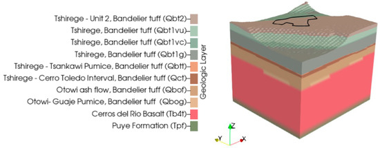
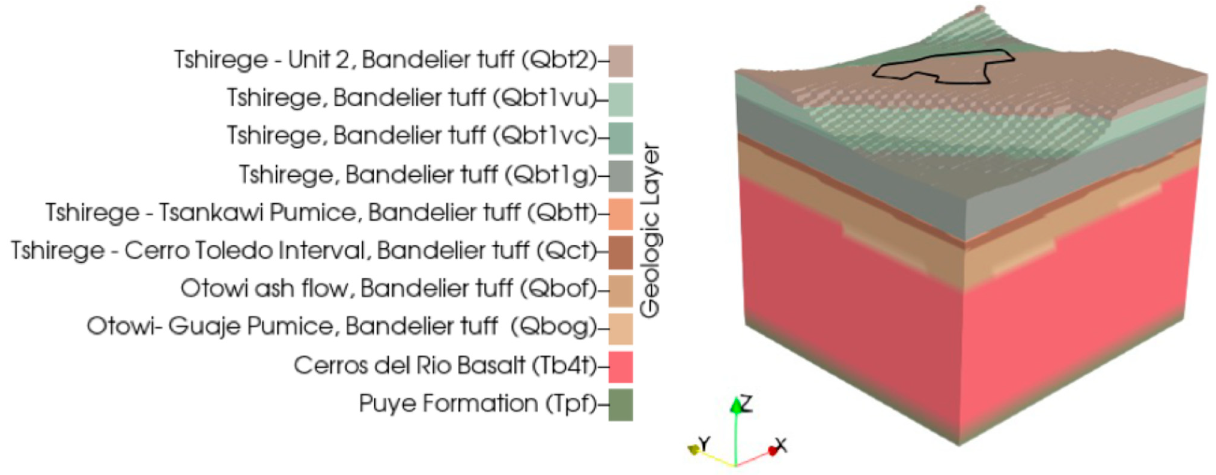
MDA L sits atop a narrow mesa with a flat surface underlain by thin, clay-rich soil and a series of volcanic ejecta. The stratigraphy is composed of Bandelier Tuff (Qbt), Cerro Toledo interval (Qct), Cerros del Rio basalt (Tb4), and Puye Formation (Tpf). A geologic framework representation of the stratigraphy is displayed in Figure 1. The Bandelier Tuffs, nearest to the surface, are composed of multiple-flow ash-and-pumice units that have heterogenous permeability based on the sequential emplacement and cooling of ash-flow tuff [16,18]. The Cerro Toledo interval is a stratified sequence of volcaniclastic sediments and tephra that separates the Tshirege member (Qbt) from the Otowi member (Qbo) of the Bandelier Tuff. Below these units lay the highly fractured Cerros del Rio basalt that comprises at least 35% of the vadose zone [17]. The basalt layer caps the top of the Puye Formation, a conglomerate of volcanic rock in a matrix of sand, silt, and clay. This layer extends from the base of the vadose zone into the saturated zone. The regional water table is estimated to be approximately 280 m (920 ft) below ground surface (bgs) [18].

Figure 1. Geologic model of the stratigraphy below MDA L (outlined in black) on the mesa.

3. Site History

MDA L is a 10,120 m² (2.5 acre) fenced area predominantly paved with asphalt that operated from the 1960s until decommissioning in the 1980s [5,9,14]. During operation, MDA L disposed of non-radioactive liquid chemical waste into unlined surface impoundments, a pit, and 34 shafts of 1 to 2 m (3 to 7 ft) diameter, 5 to 20 m (16–66 ft) deep, cutting through the youngest unit of Bandelier Tuff, the Tshirege member [5,7,14,16]. Waste was entombed in the subsurface in containers or un-containerized free release into waste disposal infrastructure. There was not sufficient documentation recorded to estimate waste volumes in the shafts [16]. Pore gas monitoring at MDA L has been required since 1985 [9]. Passive gas monitors placed on the surface around MDA L identified hot spots with VOC contamination exiting the vadose zone into the atmosphere in 1993 and 1994 [9]. A total of 28 monitoring boreholes have been drilled into the mesa to define the nature and extent of the subsurface plume. Historically, monitoring data identified TCA as the predominant VOC in the plume with the highest concentrations and greatest vertical and lateral extent [17].

In 2006 an SVE pilot test was conducted at MDA L to evaluate the effectiveness of this extraction method [17]. In this pilot test, the SVE process applied a vacuum to open boreholes in the ground where the volatile organic vapors were withdrawn and filtered using granular activated carbon at the ground surface [9,17]. The pilot test examined the potential of SVE to minimize plume growth if the source term changes substantially (e.g., one or more of the waste containers fail). An interim measure SVE operation and sequential rebound testing from 2015 to 2017 were successful in reducing the plume’s mass and mitigating VOC migration toward the water table [11]. Since then, the SVE system has been voluntarily run twice annually from 2024 to 2026 as a preventative measure to reduce VOC concentrations in the center of the plume [19]. Under non-SVE conditions, plume size is primarily controlled by diffusion away from two waste-containing-drum shaft clusters (northeast and southwest), while the atmosphere and pore water act as sinks for VOCs [12]. Aqueous transport of contaminants by unsaturated flow is not considered a viable mechanism for contaminant migration at this site since infiltration rates at mesas at LANL are generally low (<2 mm/yr) [7,13,20]. Plume rebound calculations suggest that in the absence of a catastrophic leak, the SVE system would only need to be operated for two to three months in each one-to-three-year period to retain the plume primarily within the Bandelier Tuff, well above the regional water table.

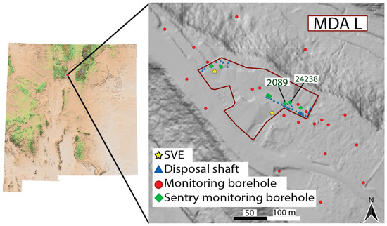
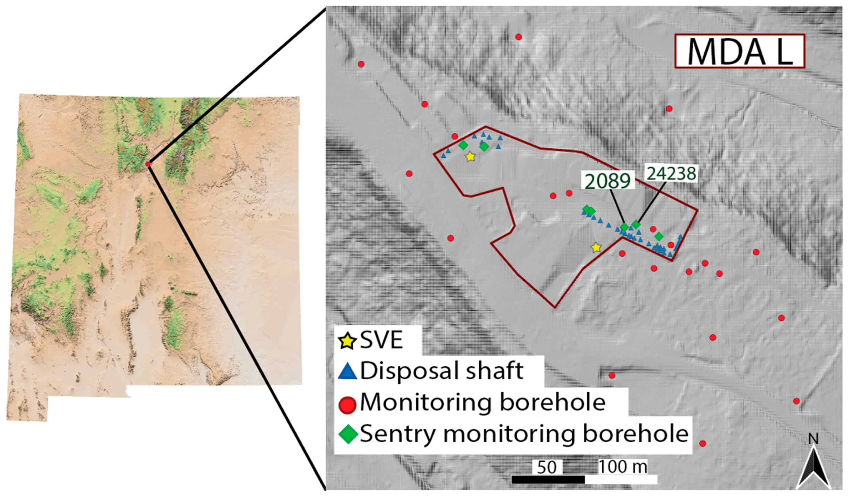
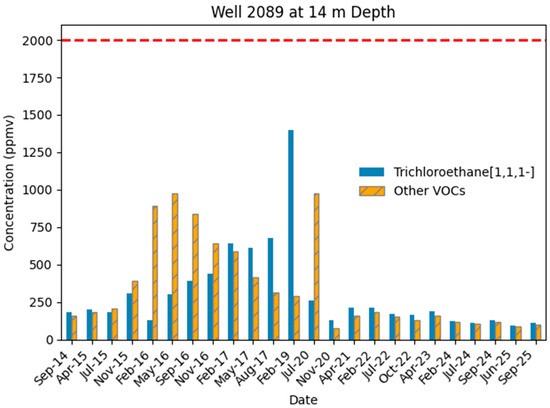
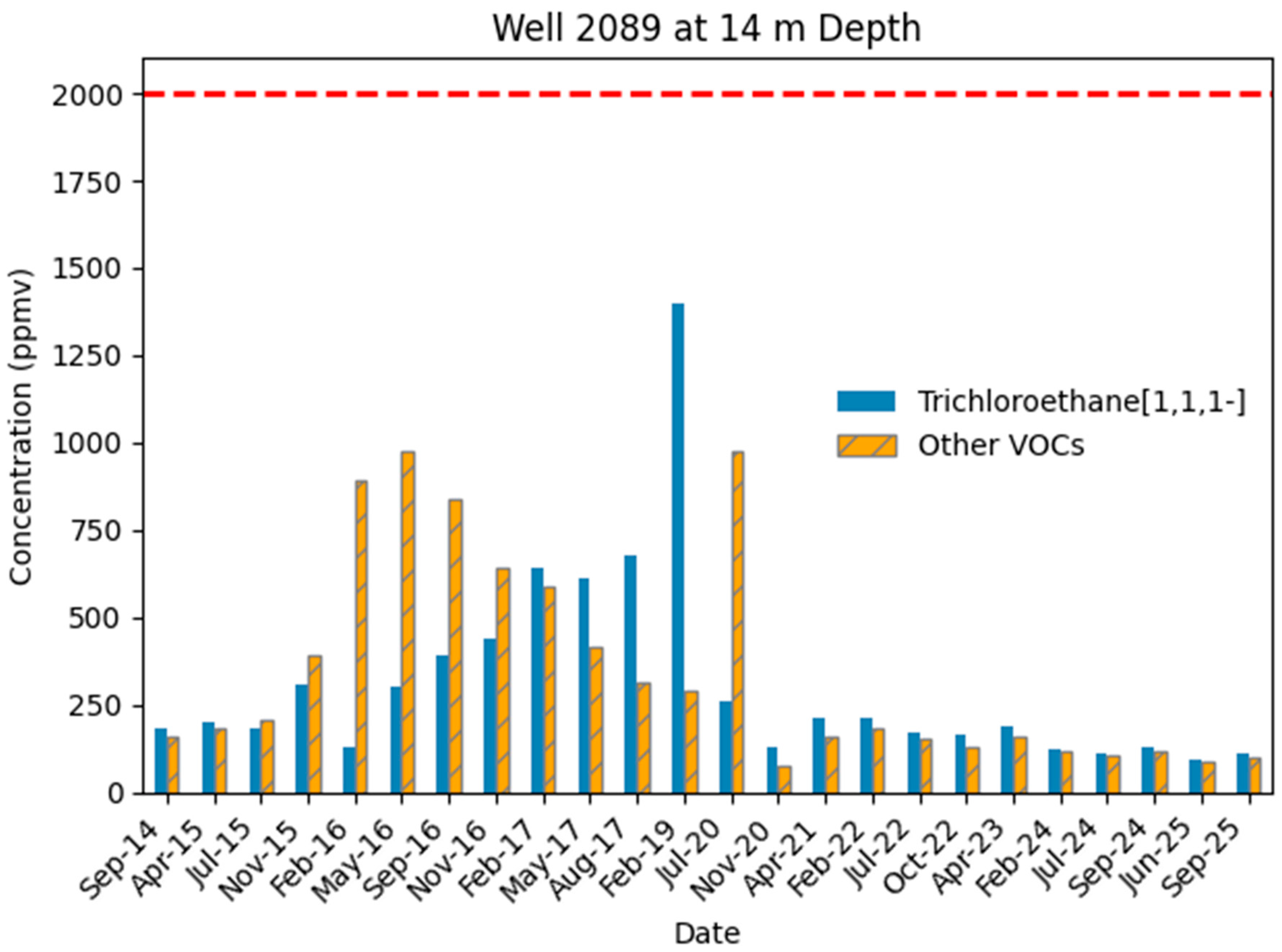
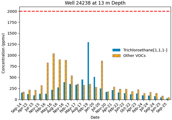
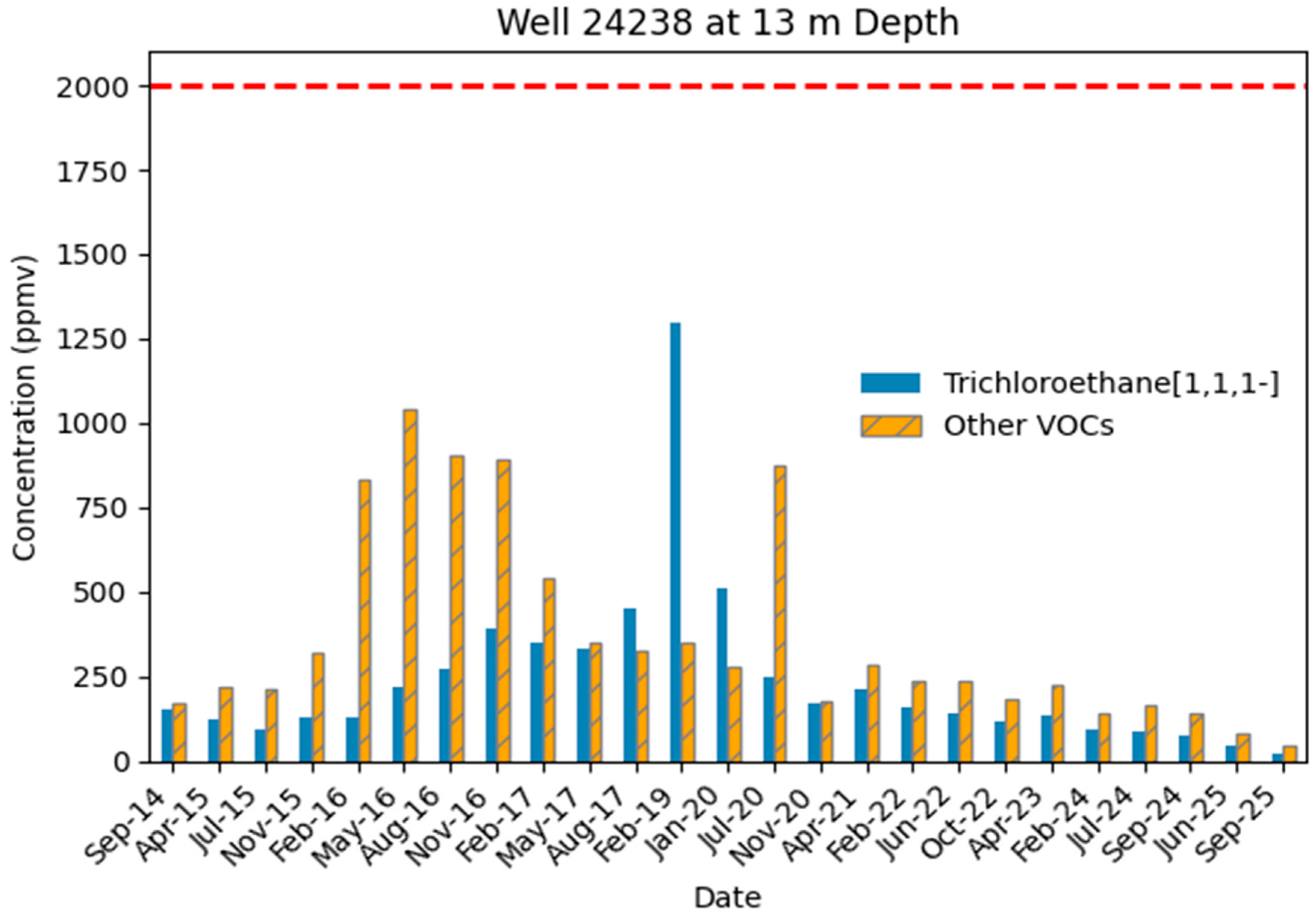
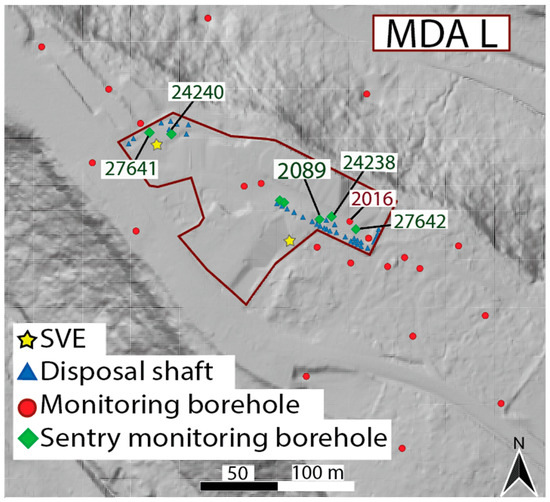
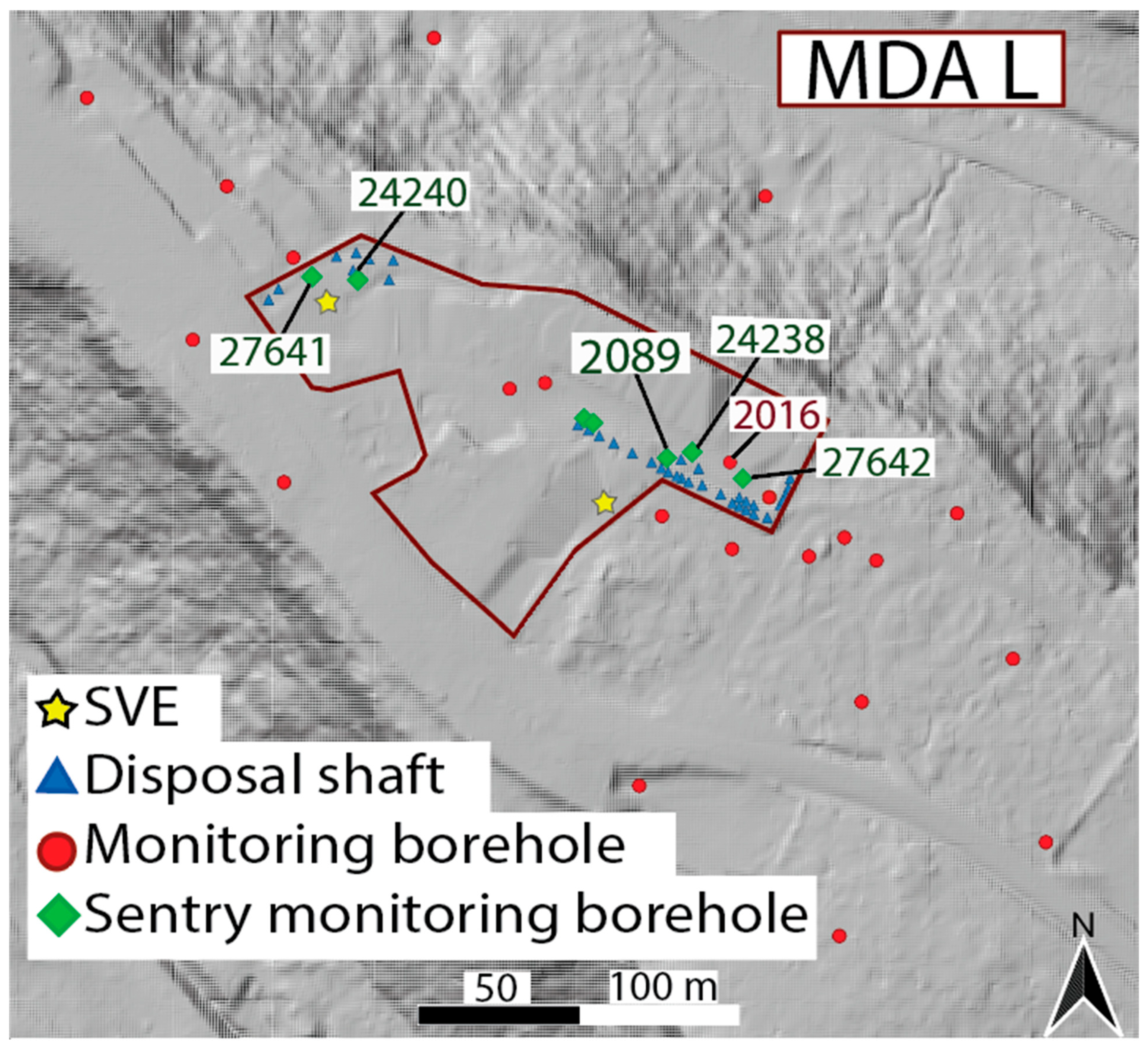
The current sampling program at MDA L reports trends in concentrations [15,19] from 28 monitoring boreholes. Seven of these monitoring boreholes are considered “sentry monitoring boreholes” (also referred to as “sentry wells”) that provide an early warning of contaminant leakage and are sampled semiannually while the other 21 monitoring wells are sampled every two years [5,19]. Previous leak modeling showed that above a threshold of 2000 parts per million by volume (ppmv) total VOC the plume could impact regional groundwater [21], thus this value was set as a trigger to activate the SVE system. Data from the 2022 MDA L Periodic Monitoring Report [15] show a noticeable increase in TCA concentrations measured in neighboring sentry monitoring boreholes 2089 and 24238 (highlighted in Figure 2, which was created using the U.S. Department of the Interior’s [22,23] publicly available data) at 14 m depth (2056 m elevation in model) which lies within the Tshirege member of Bandelier Tuff (Qbt1vc). The measured concentrations in sentry wells 2089 and 24238 increased from 640 ppmv to 1400 ppmv (Figure 3) and 350 ppmv to 1300 ppmv (Figure 4) respectively from February 2017 to February 2019. This increase has been attributed to a potential leak from source drums located near the two sentry monitoring boreholes in Figure 2. Understanding the magnitude and timing of a potential leak that could cause this increase is one of the primary purposes of our work.

Figure 2. Site located in Northern New Mexico atop a narrow mesa. MDA L is located within the maroon-colored boundary. The disposal shafts, monitoring boreholes, and SVE infrastructure are displayed using different colors and symbols. Two sentry monitoring boreholes, 2089 and 24238, are labeled on the east side. Data source courtesy of the U.S. Bureau of Land Management [22] and the U.S. Geological Survey [23].

Figure 3. Measured TCA and VOC concentrations (ppmv) at sentry well 2089 (14 m depth) from September 2014 to September 2025. SVE trigger value, 2000 ppmv, shown in red dashed line.

Figure 4. Measured TCA and VOC concentrations (ppmv) at sentry well 24238 (13 m depth) from September 2014 to September 2025. SVE trigger value, 2000 ppmv, shown in red dashed line.

4. Numerical Simulations

4.1. MDA L Model

The process of modeling MDA L began by using the Los Alamos Grid Toolbox (LaGriT) to build a computational mesh [24]. The computational mesh is used to build simulations of plume growth and subsequent SVE that are run using a finite volume multiphase simulator, the Finite Element Heat and Mass (FEHM) transfer code [5,11]. MDA L’s tetrahedral mesh is (without well refinement) composed of 142,707 primary nodes with each primary node having an associated Voronoi volume [11]. Air mass and tracer mass conservation are performed by accounting for transfer between volumes caused by pressure and concentration gradients, respectively. The minimum Voronoi volume is 12.5 m³ and the maximum Voronoi volume is 3126 m³. The mesh is 411 m long, 290 m wide, and 339.5 m in height (Figure 1). The mesh has a 10 m horizontal resolution and a varied vertical resolution. The vertical resolution is 1 m (defined by a digital elevation model) in the top 90 m, where most of the plume resides, and increases to 25 m toward the bottom of the mesh away from the VOC plume [5]. The model domain includes 10 geologic sublayers with varying saturation, permeability, porosity, and gas diffusion coefficients extending from the asphalt-covered surface to the Puye Formation (Tpf) as shown in Table 1. The gas diffusion coefficients were calculated in a 2005 paper that describes the development of MDA L as a conceptual model [11]. Permeability values were calibrated to SVE data from the 2015 interim measure [5].

Table 1. Geologic model properties.

	Density (kg/m3)	Specific Heat (J/(kg* K))	Porosity	West Permeability (m2)	East Permeability (m2)
Asphalt	1400	1000	0.5	1.75 × 10−13	1.75 × 10−13
Qbt2	1400	1000	0.41	x & y: 7.83 × 10−13 z: 5.53 × 10−13	1.00 × 10−13
Qbt1vu	1400	1000	0.49	x & y-: 7.22 × 10−12 z: 2.41 × 10−12	1.00 × 10−13
Qbt1vc	1400	1000	0.49	x & y: 1.23 × 10−13 z: 6.89 × 10−13	1.28 × 10−11
Qbt1g	1400	1000	0.46	x & y: 1.21 × 10−13 z: 6.18 × 10−13	1.00 × 10−13
Qbtt	1400	1000	0.45	6.03 × 10−13	1.00 × 10−13
Qct	1400	1000	0.45	6.03 × 10−13	1.00 × 10−13
Qbo	1400	1000	0.44	1.81 × 10−13	1.00 × 10−13
Qbog	1400	1000	0.44	1.75 × 10−13	1.75 × 10−13
Tb4t	1800	1200	0.1	1.75 × 10−13	1.75 × 10−13
Tpf	1400	1000	1	1.75 × 10−13	1.75 × 10−13

4.2. Boundary and Initial Conditions

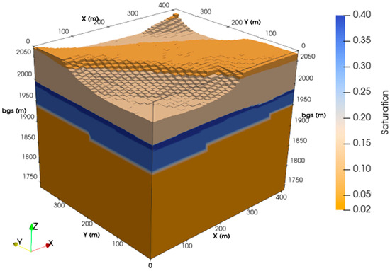
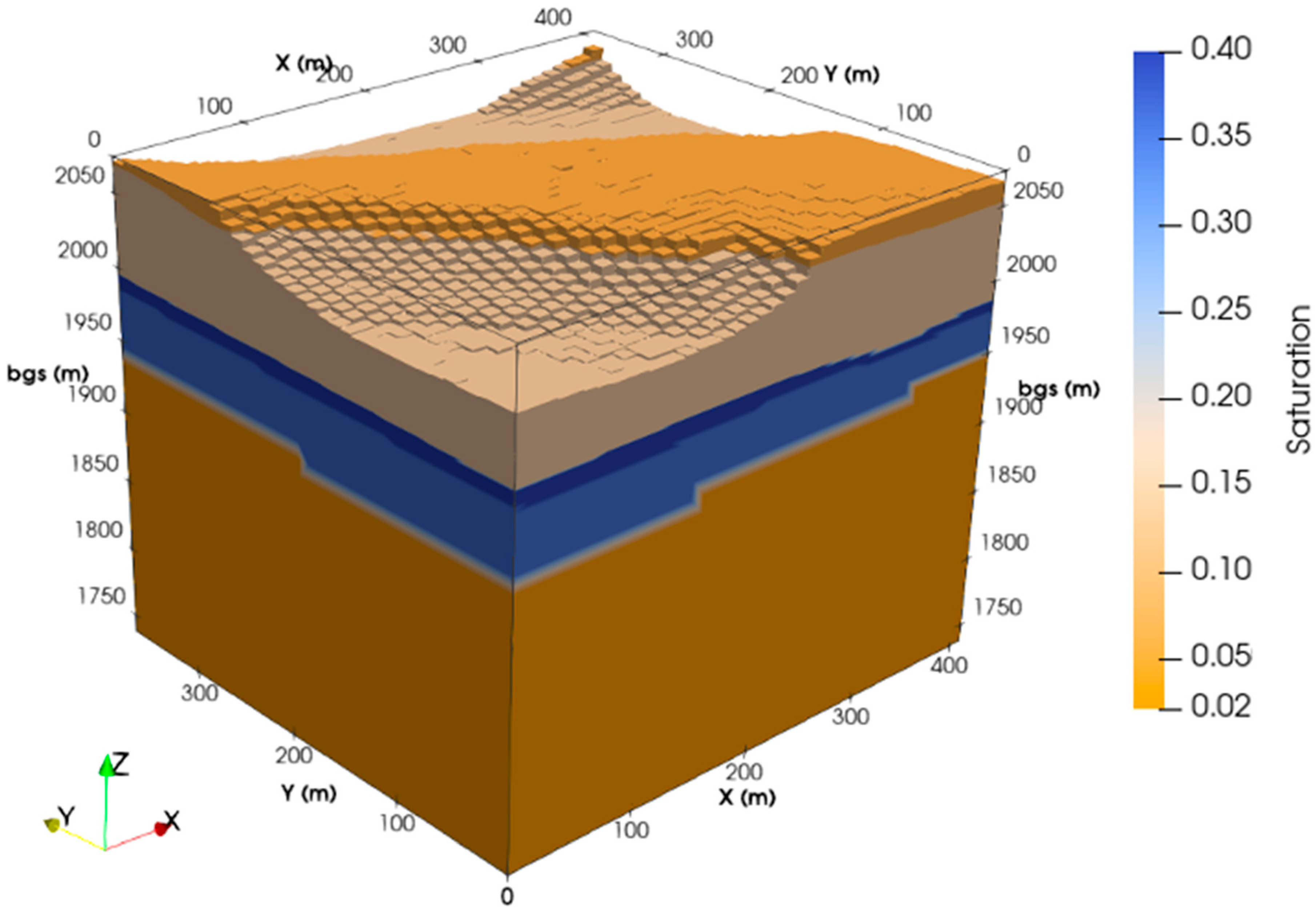
The computational mesh is populated with material properties (permeability, saturation, porosity) and TCA sources that are used to simulate changes in pressure, gas flow, and TCA concentrations. Liquid saturation remains constant in our MDA L simulations as shown in Figure 5, an assumption based on the very low water relative permeability in the tuff at the low in situ saturations [11]. The simulations are set to have isothermal gas flow with a stagnant liquid phase, a constant temperature of 15 °C, and atmospheric pressure of 0.08 MPa (Los Alamos is 80% of sea-level pressure) at the top of the domain [25]. The land surface is set to a fixed, air static pressure boundary that allows gas flow in or out of the model domain [26], with no airflow when the SVE is off. The bottom boundary of the domain (Tpf) is impermeable to water and vapor flow. Groundwater is excluded from the model, as evidenced by the saturation distributions in Figure 5. Vertically, the sides of the domain below the land surface are set to no flow for mass and heat. Long-term trends in the site monitoring data were used to set leak sources [20] along the west (shaded in gray) and east side (unshaded) of MDA L to maintain the plume in a pseudo-steady state (Table 2). See Behar 2019 for a description of drum failure probability [5].

Figure 5. Liquid saturation of MDA L model.

Table 2. Leak stage tracer (TCA) initial conditions: long-term slow leak source nodes, nearest well to the source node, model coordinates, and mass flow rates. Locations on the west side are shaded in gray and east locations are unshaded.

Long-Term Leakage Node	Nearest Well	X	Y	Z	TCA (kg/yr)
130108	27641	120	250	2055	0.20
132760	27641	120	250	2058	0.17
139195	27641	120	250	2066	0.34
130136	24240	140	260	2055	0.25
132787	24240	140	260	2058	0.21
139061	2089	230	190	2066	0.29
132594	2089	230	190	2058	0.18
129934	2089/24238	230	190	2055	0.16
129905	27642	260	180	2055	0.22
132566	27642	260	180	2058	0.23
139038	27642	260	180	2066	0.33

The boundary and initial conditions are included in the input file for each simulation using FEHM macro command statements [27]. All input decks for each simulation had the same macro commands for solvers, tolerances, and iterations. Table 3 shows the varying information included in the time macro per simulation. Additionally, automatic adaptive time stepping was used throughout where the time step is cut if the residual tolerance is exceeded. The maximum number of iterations was set to 3 in the overall Newton cycle. The maximum number of iterations for the time step size multiplier was set to 7. The time step multiplier was set to 1.8, with a minimum step size of 1.0 × 10⁻⁹.

Table 3. Time macro information per simulation.

	Leakage (July 2017–February 2019)	Passive Diffusion (February 2019–March 2023)	Passive Diffusion (March 2023–May 2024)	East SVE (May 2024)	5 min Pressure Reset	Passive Diffusion (May 2024–July 2024)
Initial time step size (days)	1	1	1	1 × 10−2	1 × 10−6	1
Final simulation time (days)	1502	3057	3408	3423	3423.0034	3470
Maximum number of time steps allowed	10,000	40,000	40,000	40,000	40,000	40,000

The tolerance used for all simulations was 1.0 × 10⁻⁶. The number of orthogonalizations in the linear equation solver was set to 40 with a maximum of 100 solver iterations per Newton iteration allowed. Since we are addressing an isothermal steady-state saturated flow, we used generalized minimum residual acceleration. The direction of the gravity vector was set as downward in the Z-direction.

The tolerances for the linear convergence and quadratic convergence for the Newton– Raphson method were set to 1.0 × 10⁻³ times the initial residual, tolerances for the residuals stopping criteria and the tolerance for each equation at each node were also set to 1.0 × 10⁻³. The over-relaxation factor was set to 1.2. Reduced degrees of freedom were not required, reordering was not done, Successive Over-Relaxation (SOR) iterations were not performed before calling the solver, and no SOR iterations were used in reduced degree of freedom methods.

Wellbores are represented in FEHM using 2-D axis-symmetric wells that couple into the primary 3-D mesh using the wellbore macro in the input file [28,29]. This well-building process is used to simulate the SVE East and SVE West pumping (calibration process is explained in [5,28] and validation in [30]). The 2-D axis-symmetric SVE wells have a central node with high permeability (10⁻⁴ m²) while the second node radially out from the center represents the casing and has a permeability of 10⁻¹⁹ m². The embedded wellbores extend from the land surface to approximately 66 m below ground surface with casing only in the top 20 m.

We use a previously calibrated 3-D SVE model of MDA L that simulated plume evolution from 2014 through June 2017 [20] to set the initial conditions for the simulations presented here. The initial conditions are set on 30 June 2017, after two days of East SVE activation and subsequent 5 min pressure reset. The initial conditions represent the subsurface TCA plume in 3-D. Additionally, the simulations include 11 TCA injection nodes (Table 2) near disposal shaft coordinates that set a slow background leakage that is required to mimic the plume data through time. Source nodes are located near monitoring/sentry wells 2089, 24238, 24240, 27641, 27642 near disposal shaft coordinate locations, Figure 6.

Figure 6. Additional sentry and monitoring well information at MDA L. Data courtesy of U.S. Geological Survey [23].

The simulations were split into three main categories: leak, passive diffusion (PD), and SVE. The simulation dates range from the end of June 2017 to July 2024. The leak phase simulates the spike measured on February 20, 2019. Because the locations of the waste shafts and impacted boreholes (2089 and 24238) are known, the available initial leakage nodes (listed in Table 2) in the 3-D model were limited. Six additional nodes near suspected disposal shafts are set as short-term leak sources in the mesh, four of which are near wells 2089 and 24238, one near 27641, and one by 24240 (new sources are bolded in Table 4). Leakage rates at these pre-selected nodes were varied manually to determine a solution that would approximately match the field data.

Table 4. Source information on the initial conditions used for each simulation (mass flow shown in kg/yr). Newly added nodes are bold. Grey highlight signifies boreholes on the west side of the site.

Nearest Well	Nodes	X	Y	Z	Leak (June 2017 to February 2019) (kg/yr)	PD (February 2019 to May 2023) (kg/yr)	PD (May 2023 to May 2024) (kg/yr)	SVE (July 2024) (kg/yr)	PD (July 2024) (kg/yr)
27641	130108	120	250	2055	0.20	0.20	0.01	0.01	0.01
27641	132760	120	250	2058	0.17	0.17	0.01	0.01	0.01
27641	136105	120	250	2062	0.13	0.85	0.00	0.00	0.00
27641	139195	120	250	2066	0.34	0.34	0.01	0.01	0.01
24240	130136	140	260	2055	0.13	0.03	0.01	0.01	0.01
24240	132787	140	260	2058	0.21	0.21	0.03	0.03	0.03
24240	136909	130	250	2063	0.01	0.04	0.00	0.00	0.00
2089	139061	230	190	2066	0.29	0.29	0.01	0.01	0.01
2089	139086	230	200	2066	0.05	0.05	0.00	0.00	0.00
2089	135164	230	200	2061	0.05	0.05	0.00	0.00	0.00
2089	132594	230	190	2058	0.18	0.18	0.07	0.07	0.07
2089	130866	230	200	2056	19.98	0.53	0.02	0.02	0.02
2089	129934	230	190	2055	0.19	0.12	0.07	0.07	0.07
2089	118841	230	200	2044	0.00	0.00	0.00	0.00	0.00
27642	129905	260	180	2055	0.02	0.02	0.02	0.02	0.02
27642	132566	260	180	2058	0.23	0.23	0.21	0.21	0.21
27642	139038	260	180	2066	0.00	0.00	0.00	0.00	0.00

The short-term leak sources used to simulate the rapid increase near well 2089 have much higher TCA mass releases per time than the passive diffusion leak sources used to model the long-term plume behavior (Table 4). A single node, 130866, accounts for most of the extra leak, as shown in Table 4. To better fit the long-term data trends, mass leakage also needed to be lowered during the passive diffusion phase for all the 17 slow leak source nodes in the model domain. Two weeks of East SVE were then simulated to match the approximate two weeks of SVE of the east well conducted in the field. A brief 5 min simulated pressure reset follows the SVE phase that allows pressure in the SVE borehole to equilibrate to an atmospheric gradient by connecting the top of the well to atmospheric pressure. Lastly, two weeks of passive diffusion were run. Measured monitoring borehole concentrations were available for February 2019, May 2023, and July 2024 (sentry wells only) and were compared to our simulated results.

5. Results and Discussion

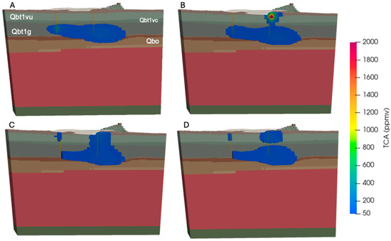
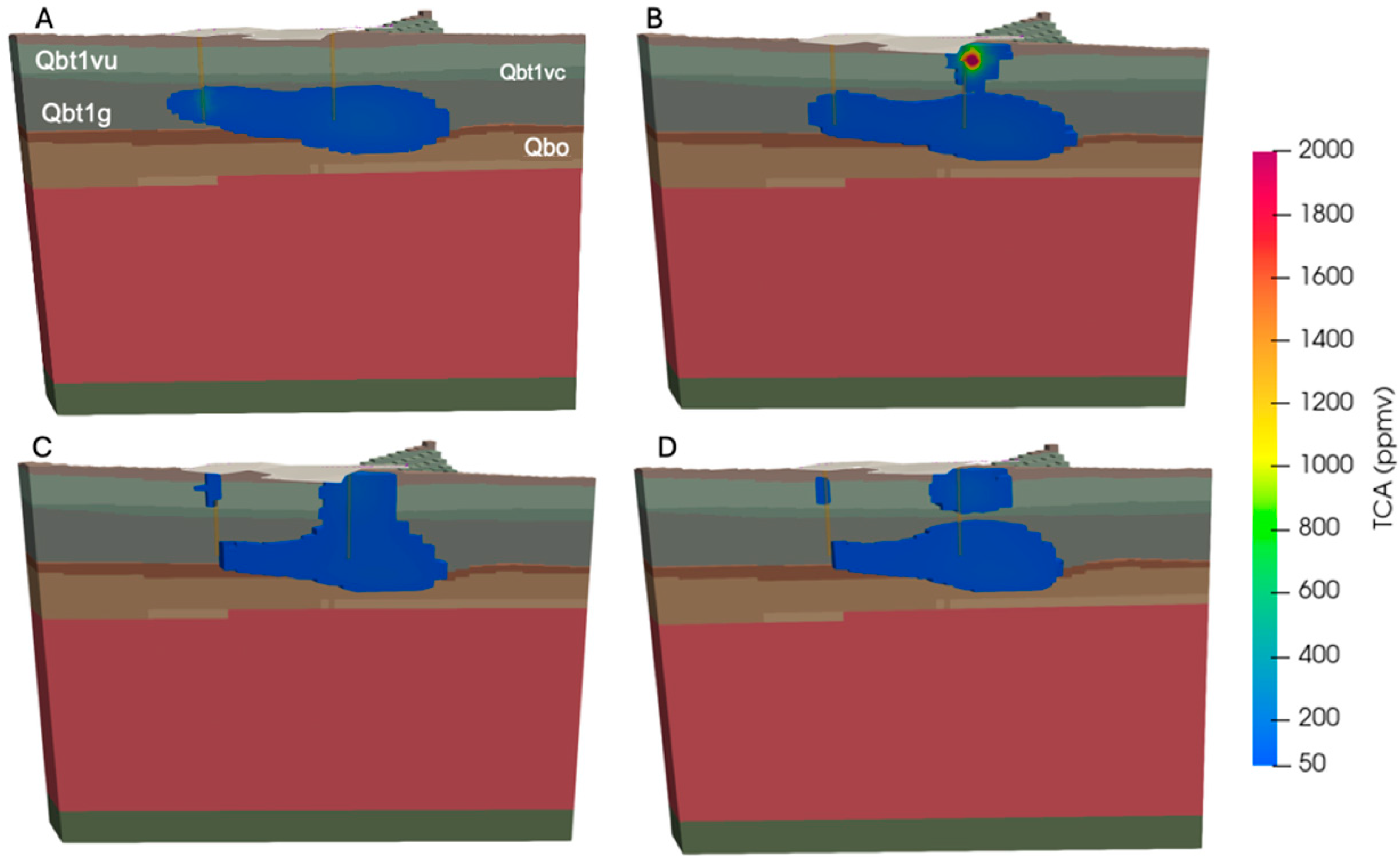
Simulating the observed concentrations allows us to determine processes that have impacted TCA plume behavior and predict the location of a potential drum failure. The simulated plume is visualized at different time steps in Figure 7. Figure 7A provides a visualization of the initial conditions where the TCA plume is two-lobed in the lower Bandelier Tuff (extending within Qbt1g to Qbo), and the highest concentration of the plume, 352 ppmv, is found on the west side of MDA L, hinted by a shade of green in Figure 7A.

Figure 7. Visualizations of the TCA plume at different timings. MDA L area is outlined in white at the surface and SVE wells are depicted in orange. Cooler shades are lower concentrations, and warmer colors are higher in concentration. (A) Initial condition (30 June 2017), (B) leak (20 February 2019), (C) end of passive diffusion post- leakage (15 May 2024), (D) post- SVE (30 May 2024). TCA concentrations truncated to only show values above 50 ppmv.

At the peak of the simulated leak, Figure 7B, a shallower plume approximately 45 m in diameter connects to the east side of the plume (~30 m depth, model Z is~2030 m) above the east lobe, showing the February 2019 leak near well 2089. One of the short-term source nodes, 130866, with the greatest mass leakage rate reached 4119 ppmv. After interpolation with nearby nodes, the average concentration at the 2089 monitoring port at model elevation 2056 m (corresponds to 14 m bgs) was 1881 ppmv. This short-duration leak remained below the SVE activation threshold value, though slightly above the measured concentration of 1400 ppmv. Other nearby wells did not have a significant impact on their concentrations by this spike. Five years of passive diffusion with the source nodes listed in Table 4 results in a shallow plume on the west side, above the west lobe (Figure 7C). New source nodes represented shallow sources in the northeast and southwest clusters. Two weeks of SVE in 2024 generally lowered the overall concentration of the plume. Visually, the more permeable unit (Qbt1vc) explains separation of the plume on the east side in Figure 7D. The top plume has the higher concentration of 132 ppmv. The morphology and connectivity of the plume over time can be best explained by the permeabilities of Tshirege members below Unit-2 (Qbt2, above Qbt1vu) that support good eastward vertical fluid flow at Qbt1vc. Despite individual source nodes surpassing the threshold, the plume returns to background concentrations over time, as seen in Figure 7D.

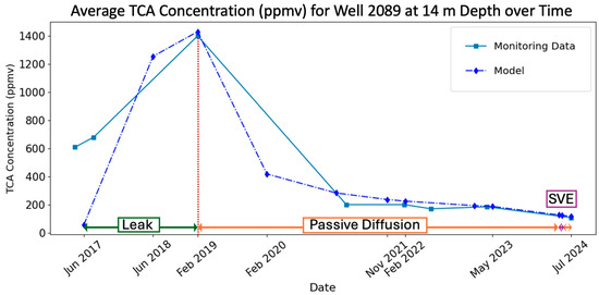
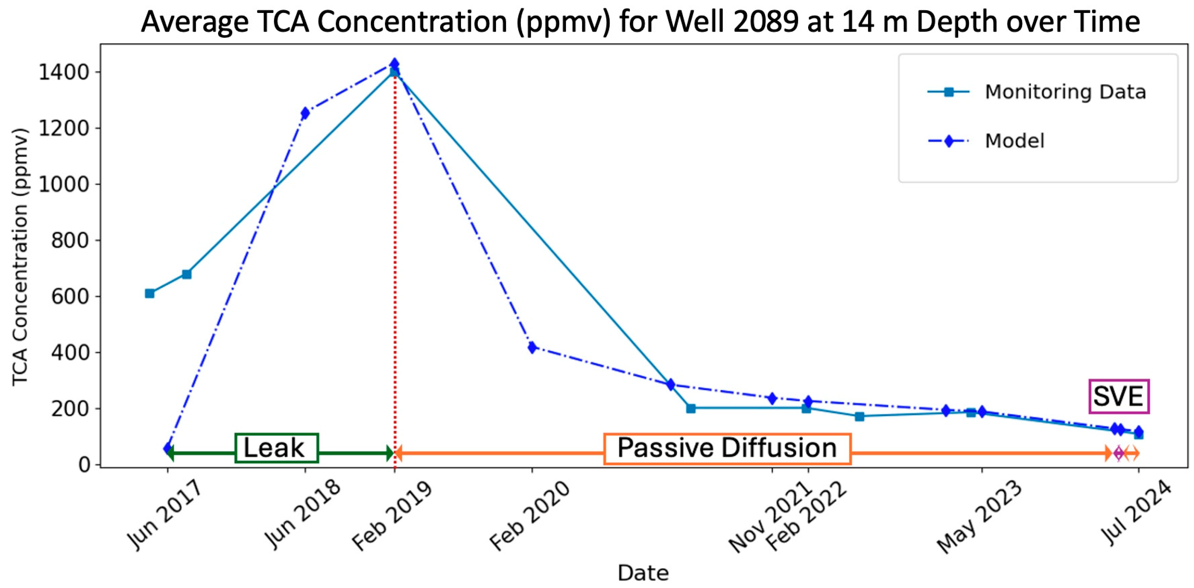
A nearest neighbor interpolation was used with the simulation results to get the average concentration at the corresponding depths along monitoring wells. These simulation results were compared to measured concentrations in monitoring boreholes along different depths. Many manual iterations were performed, adjusting leak rates to create a simulation that primarily agreed with the measured data for increasing concentrations near borehole 2089 while achieving alignment with the rest of the model domain as a secondary goal. Figure 8 is a time series comparing modeled and measured sentry well 2089 concentrations. Generally, the simulation trends match well with the data for sentry well 2089 at 14 m (2056 m in the model) depth as highlighted in Figure 8 from June 2017 to July 2024. The initial conditions for these runs were set in June 2017, after 24 days of SVE, explaining the concentration mismatch at the start date at this depth.

Figure 8. Time series comparison of TCA concentrations at sentry well 2089 at 14 m depth to measured concentrations. The three stages—leak, passive diffusion, and SVE—are color-coded in green, orange, and purple, respectively. The red vertical dotted line represents the date of the measured spike, which corresponds to the monitoring round with the largest leakage signal.

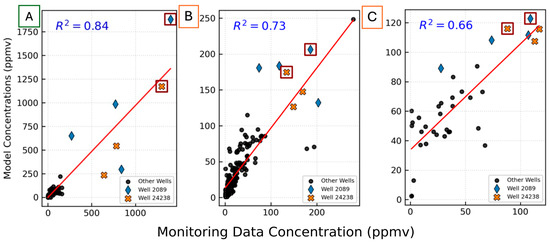
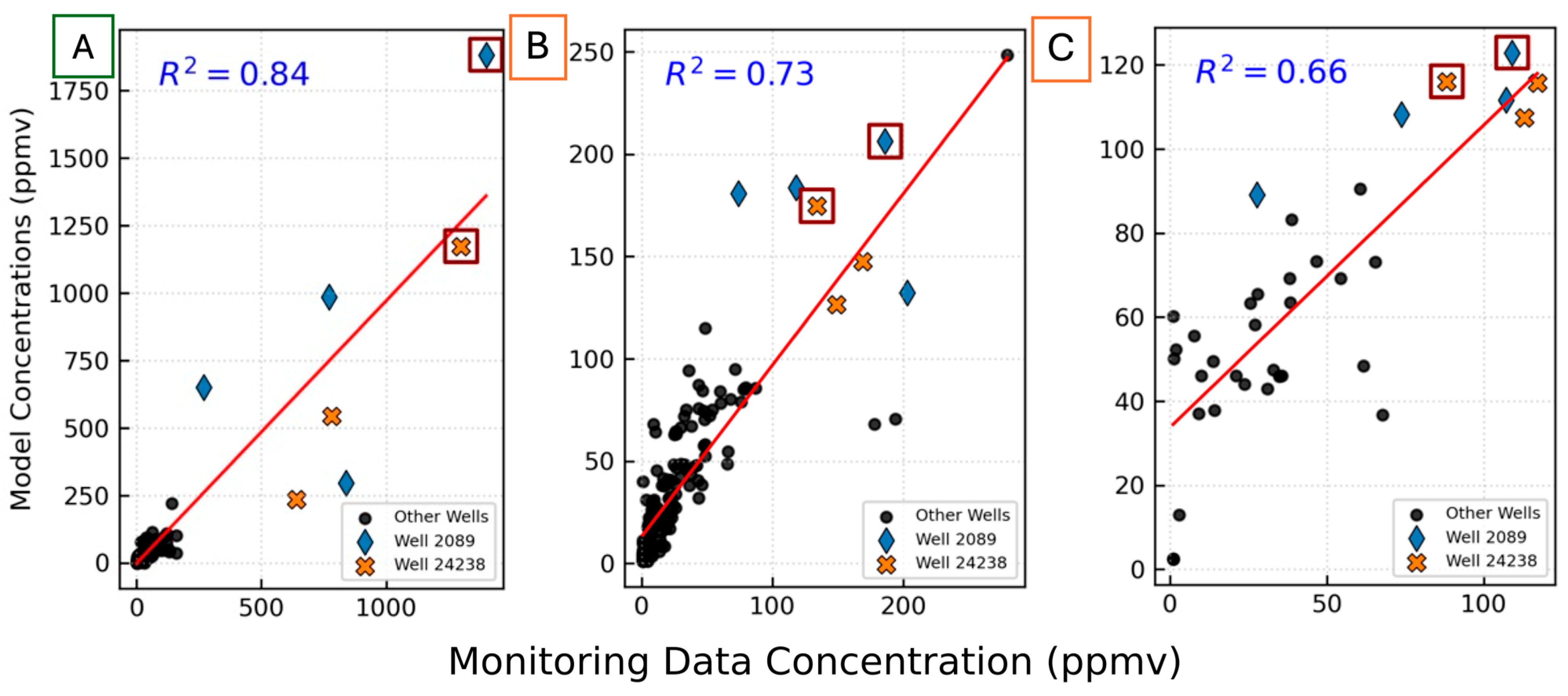
Figure 9 shows three regression plots between the model concentrations and monitored concentrations. It highlights the coefficient of determination (R²) for leakage in February 2019 and two passive diffusion stages in March 2023 and July 2024 (post-SVE). The linear regression plots indicate concentrations for sentry wells 2089 and 24238 at 14 m depth outlined with maroon boxes. The leak phase axes differ in range where the model’s maximum (y-axis) is above 1750 ppmv and the monitoring maximum (x-axis) is 1400 ppmv. Plots B and C show similar axis ranges around 250 ppmv and 120 ppmv, respectively, showing a contrast between concentration maximums in the model and those measured in the field.

Figure 9. Linear regression plots (A,B,C) of model concentrations versus monitored concentrations. Stages: leak and passive diffusion have color-coded boundaries of green and orange, respectively, around A, B, and C labels. Regression plots for (A) February 2019 (R² = 0.84), (B) March 2023 (R² = 0.73), and (C) July 2024 (R² = 0.66). Sentry wells 2089 and 24238 are marked by a blue diamond and orange cross, respectively. Boxed markers are data points at 14 m depth.

The regression analyses indicate a gradual decline in predictive agreement between simulated and observed data over time. The later R² values are less important since the goal of the proof-of-concept is to generate a leak signal that responds approximately like the data at wells 24238 and 2089 during the 2017 to 2020 period. After simulating the larger leak, all leakage source concentrations were dropped back down to background levels. The concentrations for wells 2089 and 24238 are both overestimated and underestimated at different depths. In Figure 9B the two points below the symbolled points were underestimated by the model and represent 24240 on the west side. All the data points in Figure 9C refer to sentry monitoring boreholes only (as opposed to all monitoring boreholes). Our efforts prioritized simulating the leak that resulted in the highest measured concentration in February 2019. Expanding the focus of this paper to sentry wells on the west side could ameliorate the decreasing trend in correlation coefficients.

Next, we explore the total mass injected and produced near borehole 2089 at each stage. All mass produced out of the model domain either diffuses out of the top boundary to the zero-concentration atmospheric boundary or is pulled into the SVE wells when they are operating. Approximately 34 kg of TCA is added to the model domain in the simulated leak around wells 2089 and 24238 from June 2017 to February 2019. This represents 93% of simulated TCA leakage in the model domain during this time, 13 times greater than the previously calibrated simulated background leakage. Later in May 2024, two weeks of simulated SVE on the east well removed 16 kg of TCA from the model domain. The initial mass of TCA in the model domain was 415 kg; post-leak the total TCA mass in the model domain was 447 kg. Post-SVE and short-term rebound resulted in the final mass of 415 kg in the model domain. Despite a brief leak within the model, the SVE method was successful in bringing concentrations back to near their initial values. However, the decrease in the regression analyses over time highlights that the example leak is not an ideal solution, but a useful proof-of-concept to guide the next steps in numerical site analysis. Further development, including uncertainty quantification and AI/ML, will rely on cost–benefit analysis by the site operators.

Integrating across the total model domain, from July 2017 to July 2024 the total amount of TCA leaked into the model domain was 51.2 kg while 51.6 kg was extracted/produced. The breakdown of these values is provided in Table 5. The net mass balance error was calculated per simulation as follows:

Net Mass Balance Error = (Current Mass − Initial Mass) − (Total Injected
Mass − Total Produced Mass),

(1)

Table 5. Model domain mass changes per simulation.

	Leakage (July 2017–February 2019)	Passive Diffusion (February 2019–March 2023)	Passive Diffusion (March 2023–May 2024)	East SVE (May 2024)	Passive Diffusion (May 2024–July 2024)
Total injected mass into model (kg)	36.49	14.17	0.45	0.02	0.06
Total produced mass out of model (kg)	4.64	24.11	6.05	16.22	0.59
Mass leaked near 2089 (kg)	34.11	5.23	0.17	0.01	0.02
Net mass change (kg)	31.85	−9.94	−5.60	−16.20	−0.53
Net mass balance error (kg)	2.15 × 10−5	−1.40 × 10−5	1.85 × 10−6	3.75 × 10−3	−8.53 × 10−6

To match the observed concentrations, it was necessary to drop the source concentrations significantly by the final time step, explaining the larger amount of TCA removed from the model compared to the amount leaked into the model domain. This further highlights the short-term leak impacts on plume behavior in the subsurface at MDA L.

6. Conclusions

A new method at this site for estimating subsurface leakage at LANL’s MDA L using discrete container failures within a previously calibrated 3-D SVE model is presented and validated using site monitoring data. Simulations show that a short-term leak of approximately 34 kg of TCA can approximately explain the increase in observed concentrations in monitoring data at boreholes 2089 and 24238, located within 4–8 m of the simulated leak. The simulations show that TCA concentrations remained below the SVE trigger value of 2000 ppmv at monitoring locations since 2017. The plume not only remains well above the regional aquifer, but it also maintains concentrations below the SVE trigger value despite new short-term leak sources. The plume starts as double-lobed within the lower Bandelier Tuff (Qbt1g, Qbtt, and Qct). Post-leakage, plume expansion evolves closer to the surface at both disposal shaft clusters. Separation of the plume post-east SVE activation within the model occurs along the Tshirege member (Qbt1vc) of the Bandelier Tuff and can be explained by the differences in permeability. This proof-of-concept study highlights the usefulness of calibrated 3-D numerical simulations to understand changes in site monitoring data and assign order of magnitude estimates to short-term VOC container leaks. The work further highlights the success of the current remediation plan in response to waste container failure. The new method presented for estimating leakage at MDA L in an active site provides impetus for other sites to build calibrated 3-D models that can be adapted as new needs will inevitably arise.

References

- Huang, B.; Lei, C.; Wei, C.; Zeng, G. Chlorinated volatile organic compounds (Cl-VOCs) in environment—Sources, potential human health impacts, and current remediation technologies. Environ. Int. 2014, 71, 118–138. [Google Scholar] [CrossRef] [Scilit] [PubMed]
- Pandey, P.; Yadav, R. A review on volatile organic compounds (VOCs) as environmental pollutants: Fate and distribution. Int. J. Plant Environ. 2018, 4, 14–26. [Google Scholar] [CrossRef] [Scilit]
- Noonkester, J.V.; Nichols, R.L.; Dixon, K.L. Innovative Technologies and Vadose Zone Treatment of Chlorinated Volatile Organic Compounds—Case Study. Environ. Geosci. 2005, 12, 219–233. [Google Scholar] [CrossRef] [Scilit]
- Oostrom, M.; Truex, M.J.; Tartakovsky, G.D.; Wietsma, T.W. Three-dimensional simulation of volatile organic compound mass flux from the vadose zone to groundwater. Groundw. Monit. Remediat. 2010, 30, 45–56. [Google Scholar] [CrossRef] [Scilit]
- Behar, H.R.; Snyder, E.E.; Marczak, S.; Salazar, L.J.; Rappe, B.; Fordham, G.F.; Chu, S.P.; Strobridge, D.M.; Birdsell, K.H.; Miller, T.A.; et al. An Investigation of Plume Response to Soil Vapor Extraction and Hypothetical Drum Failure. Vadose Zone J. 2019, 18, 1–21. [Google Scholar] [CrossRef] [Scilit]
- Lei, X.; Cheng, H.; Peng, J.; Jiang, H.; Lyu, X.; Zeng, P.; Wang, Z.; Guo, H. Impact of long-range atmospheric transport on volatile organic compounds and ozone photochemistry at a regional background site in central China. Atmos. Environ. 2021, 246, 118093. [Google Scholar] [CrossRef] [Scilit]
- Riley, R.G. Arid Site Characterization and Technology Assessment: Volatile Organic Compounds—Arid Integrated Demonstration; Technical Report; Pacific Northwest Laboratory: Richland, WA, USA, 1993. [Google Scholar]
- Baker, R.J.; Andraski, B.J.; Stonestrom, D.A.; Luo, W. Volatile Organic Compounds in the Unsaturated Zone from Radioactive Wastes. J. Environ. Qual. 2012, 41, 1324–1336. [Google Scholar] [CrossRef] [Scilit] [PubMed]
- Northern New Mexico Citizens’ Advisory Board (NNMCAB). Recommendation to the Department of Energy No. 2010-05: Recommendation for Interim Measure for Volatile Organic Constituent Contaminant Source Removal in MDA-L and MDA-G.; Drafted by the Combined Environmental Monitoring, Surveillance and Remediation and Waste Management Committees; NNMCAB: Los Alamos, NM, USA, 2010. Available online: https://www.energy.gov/node/1140771 (accessed on 20 April 2026).
- Carroll, K.C.; Truex, M.J.; Brusseau, M.L.; Parker, K.R.; Mackley, R.D.; Rohay, V.J. Characterization of persistent volatile contaminant sources in the vadose zone. Groundw. Monit. Remediat. 2013, 33, 68–84. [Google Scholar] [CrossRef] [Scilit]
- Stauffer, P.H.; Birdsell, K.H.; Witkowski, M.S.; Hopkins, J.K. Vadose Zone Transport of 1,1,1-Trichloroethane: Conceptual Model Validation through Numerical Simulation. Vadose Zone J. 2005, 4, 760–773. [Google Scholar] [CrossRef] [Scilit]
- Snyder, E.E.; Marczak, S.; Salazar, L.; Fordham, G.; Chu, S.; Birdsell, K.; Rich, K.; Stauffer, P. The Impact of Soil Vapor Extraction at Material Disposal Area L, Los Alamos National Laboratory; Paper No. 17155. In Proceedings of the 2017 Waste Management Symposia, Phoenix, AZ, USA, 5–9 March 2017. [Google Scholar]
- Stauffer, P.H.; Hopkins, J.K.; Anderson, T.; Vrugt, J. Soil Vapor Extraction Pilot Test at Technical Area 54, Material Disposal Area L: Numerical Modeling in Support of Decision Analysis; Los Alamos National Laboratory: Los Alamos, NM, USA, 2007. [Google Scholar]
- National Research Council. Plans and Practices for Groundwater Protection at the Los Alamos National Laboratory: Final Report; National Academies Press: Washington, DC, USA, 2007. [Google Scholar]
- Newport News Nuclear BWXT–Los Alamos, LLC (N3B). Periodic Monitoring Report for 2022 Vapor-Sampling and Soil-Vapor Extraction at Material Disposal Area L, Solid Waste Management Unit 54-006, at Technical Area 54, Los Alamos, New Mexico; Report No. EM2023-0049; N3B: Los Alamos, NM, USA, 2023. [Google Scholar]
- Anderson, T.; Stewart, B.; Mark, P.; Stauffer, P.; Hopkins, J. A Soil Vapor Extraction Pilot Study in a Deep Arid Vadose Zone, Part I: Field Study Summary. In Proceedings of the 2007 Waste Management Symposia, Tucson, AZ, USA, 25 February–1 March 2007. [Google Scholar]
- Environmental Programs Directorate. Periodic Monitoring Report for Vapor Sampling Activities at MDA L for Second Quarter FY08; Report No. LA-UR-08-4761; Los Alamos National Laboratory: Los Alamos, NM, USA, 2008. [Google Scholar]
- Environmental Programs Directorate–LANL Water Stewardship Project. 2009 Hydrogeologic Site Atlas; Report No. LA-UR-09-3763/EP2009-0191; Los Alamos National Laboratory: Los Alamos, NM, USA, 2009. [Google Scholar]
- Newport News Nuclear BWXT–Los Alamos, LLC (N3B). Periodic Monitoring Report for 2024 Vapor-Sampling and Soil-Vapor Extraction at Material Disposal Area L, Solid Waste Management Unit 54-006, at Technical Area 54, Los Alamos, New Mexico; Report No. EM2025-0239; N3B: Los Alamos, NM, USA, 2025. [Google Scholar]
- Kwicklis, E.; Witkowski, M.; Birdsell, K.; Newman, B.; Walther, D. Development of an Infiltration Map for the Los Alamos Area, New Mexico. Vadose Zone J. 2005, 4, 672–693. [Google Scholar] [CrossRef] [Scilit]
- Newport News Nuclear BWXT–Los Alamos, LLC (N3B). Interim Measures Final Report for Soil-Vapor Extraction of Volatile Organic Compounds from Material Disposal Area L, Technical Area 54, Revision 1; Report No. EM2022-0290; N3B: Los Alamos, NM, USA, 2022. [Google Scholar]
- U.S. Department of the Interior, Bureau of Land Management (BLM). RGIS. Available online: https://rgis.unm.edu/rgis6/ (accessed on 10 August 2024).
- U.S. Department of the Interior, U.S. Geological Survey (USGS). 3DEP LidarExplorer. Available online: https://apps.nationalmap.gov/lidar-explorer/#/ (accessed on 10 August 2024).
- Miller, T.A.; Vesselinov, V.V.; Stuaffer, P.H.; Birdsell, K.H.; Gable, C.W. Integration of Geologic Frameworks in Meshing and Setup of Computational Hydrogeologic Models, Pajarito Plateau, New Mexico. In New Mexico Geological Society Guidebook, 58th Field Conference: Geology of the Jemez Mountains Region III; New Mexico Geological Society: Socorro, NM, USA, 2007; pp. 121–128. [Google Scholar]
- Sulca, D.; Stauffer, P.H.; Ahmmed, B.; Hobbs, N.; Reid, K. Characterizing Contaminant Transport at Los Alamos National Laboratory Using a Vadose Zone Vapor Plume Model; Paper No. 25462. In Proceedings of the 2025 Waste Management Symposia, Phoenix, AZ, USA, 9–13 March 2025. [Google Scholar]
- Stauffer, P.H.; Rosenberg, N.D. Vapor Phase Transport at a Hillside Landfill. Environ. Eng. Geosci. 2000, 6, 71–84. [Google Scholar] [CrossRef] [Scilit]
- Input Data. Available online: https://lanl.github.io/FEHM/program-specification/input-data#alpha-macro (accessed on 21 May 2026).
- Stauffer, P.H.; Hopkins, J.K.; Anderson, T. A Soil Vapor Extraction Pilot Study in a Deep Arid Vadose Zone, Part 2: Simulations in Support of Decision Making Processes. In Proceedings of the 2007 Waste Management Symposia, Tucson, AZ, USA, 25 February–1 March 2007. [Google Scholar]
- Dash, Z.V.; Robinson, B.A.; Pawar, R.J.; Chu, S. Software Validation Report for the FEHM Application Version 3.1—3.X, Report (LA-UR-15-27776); Los Alamos National Laboratory: Los Alamos, NM, USA, 2015. [Google Scholar]
- Pawar, R.J.; Zyvoloski, G.A. A novel method to couple wellbore flow to reservoir flow. In Proceedings of the 16th International Conference on Computational Methods in Water Resources (CMWRXVI), Copenhagen, Denmark, 19–22 June 2006. LA-UR-06-3956. [Google Scholar]
Disclaimer/Publisher’s Note: The statements, opinions and data contained in all publications are solely those of the individual author(s) and contributor(s) and not of MDPI and/or the editor(s). MDPI and/or the editor(s) disclaim responsibility for any injury to people or property resulting from any ideas, methods, instructions or products referred to in the content. |
© 2026 by the authors. Licensee MDPI, Basel, Switzerland. This article is an open access article distributed under the terms and conditions of the Creative Commons Attribution (CC BY) license.