


Abstract
Travel–time-based thermal tracer tomography (TTT) has emerged as a promising technique for characterizing aquifer heterogeneity. However, the influence of travel–time definitions and data density on inversion performance is not well understood. In this study, we present a controlled two-dimensional sandbox experiment designed to systematically investigate three travel–time definitions (early-time t10, intermediate t50, and peak-time tpeak) under data-rich (32 travel times) and data-sparse (10 travel times) conditions. The obtained hydraulic conductivity (K) fields are benchmarked against permeameter measurements and a geostatistical inversion that assimilates dense steady-state head observations. The results demonstrate that all three travel–time definitions satisfactorily reproduce the primary layered heterogeneity when abundant travel–time data are available, with t50 and tpeak providing marginally better structural fidelity under data-rich conditions. However, only the early-time t10 definition preserves the spatial continuity of dominant geological structures under data-sparse conditions, exhibiting superior robustness. All TTT inversions systematically underestimate the K ranges and exhibit pronounced range compression, whereas the geostatistical inversion overestimates K and introduces spurious high-value extremes. Forward thermal transport simulations reveal that TTT-derived K fields yield systematically delayed thermal breakthroughs, while the geostatistical inversion yields more accurate predictions. These findings highlight the critical interplay between travel–time diagnostics and observation density. They also underscore the necessity of jointly inverting hydraulic and thermal data to overcome the limitations of single-dataset approaches for reliable aquifer characterization and transport prediction.
1. Introduction
Aquifer heterogeneity fundamentally controls groundwater flow and solute transport, governing preferential flow paths, plume migration, and heat transfer [1,2,3]. Among the inverse methods developed to characterize such heterogeneity, hydraulic tomography (HT) uses pressure responses from cross-well pumping tests to resolve spatial variations in hydraulic properties [4,5,6,7,8]. Tracer-based approaches [9,10,11], especially thermal tracer tomography, exploit temperature signals from heat injections to reconstruct subsurface hydraulic conductivity (K) distributions [12,13,14,15,16,17,18,19,20]. Geostatistical inversion provides another widely used framework that integrates observational data with spatial covariance models [21,22,23,24,25,26], and it has been validated in both sandbox and field settings [10,27,28]. Although numerical studies [15,16,17,29] and field experiments [18,19,30,31] have demonstrated the potential of these techniques, the lack of controlled ground truth often limits quantitative assessment of reconstruction fidelity.
Laboratory sandbox experiments provide a unique intermediate scale at which the true heterogeneity is known, and both hydraulic and thermal signals can be captured at high resolution [10,24]. Sandbox studies have successfully validated HT and geostatistical inversion, demonstrating their ability to recover heterogeneous structures and to predict solute transport [10,11,27,32,33]. Tracer tomography using gas tracers has also been demonstrated at the laboratory scale in fractured rock samples [11]. Despite these advances, travel-time-based thermal tracer tomography (TTT) has not yet been systematically evaluated in a controlled sandbox setting. Consequently, several key methodological questions remain open.
Previous TTT studies have primarily relied on numerical simulations [17,20] or field tests [18,19,34], where the true K field remains uncertain. In particular, the influence of travel–time definitions (e.g., early-time t10, intermediate t50, and peak-time tpeak) and observation density on the recovered heterogeneity structure and parameter range has not been isolated under known conditions. Without controlled experiments, it remains unclear which travel–time strategy best preserves spatial continuity under data-sparse conditions. To address this gap, we provide the first laboratory evaluation of TTT using a well-characterized heterogeneous sandbox. This enables direct assessment of both structural recoverability and parameter range recovery against known K distributions.
Using a controlled sandbox experiment, this study investigates the capability of TTT to recover aquifer heterogeneity under varying data densities and travel–time definitions.
Following this introduction, Section 2 describes the sandbox model and the experimental setup, Section 3 introduces the inversion method and the setup of travel–time strategy, Section 4 presents and discusses the experimental and reconstruction results, and Section 5 summarizes the main conclusions.
2. Laboratory Sandbox Experiment
2.1. Sandbox Model
A laboratory sandbox (120 cm × 60 cm × 10 cm) was employed to construct a two-dimensional heterogeneous aquifer. The left and right boundaries were maintained at constant heads via two reservoirs to establish the desired hydraulic gradient, while the other four sides were sealed as no-flow boundaries, as described in detail by Qiu et al. (2025) [33].
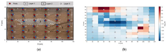
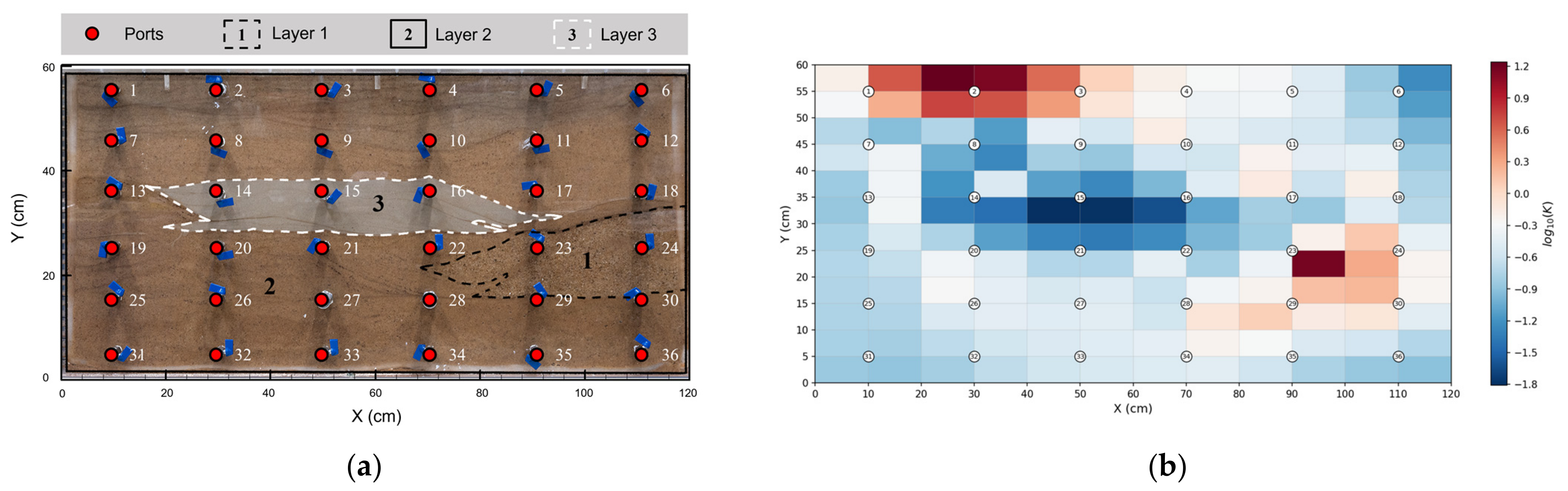
The heterogeneous aquifer was built by alternately depositing three sand grades under controlled flow conditions (Illman et al., 2010 [24]), yielding three distinct layers. These layers are designated as Layers 1, 2, and 3 (Figure 1a). Layer 2 serves as the background matrix and occupies the majority of the apparatus, except for Layer 1 (bottom right) and Layer 3 (middle section). Figure 1b illustrates the geostatistical inversion result based on previous studies by Qiu et al. (2025) [33]. The high-permeability zone in the upper-left corner (x = 10–50 cm; y = 50–60 cm) represents an unexpected deviation from the intended uniform fill, reflecting localized heterogeneity identified by the inversion.
Figure 1.
(a) Photograph of the laboratory sandbox with a three-layer synthetic heterogeneous aquifer (Reproduced from Qiu et al., 2025 [33], with permission from Elsevier); (b) geostatistical inversion result.
The three-layer configuration adopted here represents a simplified heterogeneity structure. This approach follows the established sandbox methodology in which layered heterogeneity with known properties is used to isolate specific inversion mechanisms under controlled ground-truth conditions [24,32,33]. This simplification enables unambiguous attribution of inversion artifacts to methodological factors (travel-time definition, data density) rather than to unresolved geological complexity. However, the advection-to-diffusion ratio may differ between this simplified system and natural aquifers with multi-scale, hierarchical heterogeneity. The quantitative metrics, such as the degree of K-range compression and breakthrough curve (BTC) delay magnitude, are therefore likely structure-dependent and should be recalibrated for field applications.
Locally, alternating layers of high- and low-permeability media were constructed near Ports 22 and 23. Additionally, a high-permeability zone was created in the upper-left area (Ports 1, 2, and 3), representing a complex structural feature.
For monitoring, 36 ports with pressure sensors on the front side and 16 ports with temperature sensors on the back side were installed throughout the aquifer. Each port has a diameter of 1.2 cm.
The grain size, dry density, porosity, and permeameter-derived K values of the three sands are summarized in Table 1. Detailed measurement procedures are provided in Supplementary Materials, which follow those reported in Qiu et al. (2025, Table 1) [33]. The aquifer was characterized by different approaches, as outlined in the sections that follow.
Table 1.
Physical properties of the three sand materials used for constructing the heterogeneous aquifer (Reproduced from Qiu et al., 2025 [33], with permission from Elsevier).
2.2. Experimental Setup and Data Collection
Sixteen cross-port pumping tests were performed across the aquifer (Ports 8–11, 14–17, 20–23, and 26–29). Pressure responses at all 36 ports were recorded with 0–20 kPa transducers; measurements from the topmost and bottommost ports were discarded due to excessive noise, leaving 24 reliable transducers. Full test details are provided in Qiu et al. (2025) [33].
Four thermal tracer tests were carried out at Ports 8, 14, 20, and 26, with temperature data collected at 16 monitoring ports (Ports 8–11, 14–17, 20–23, and 26–29) for thermal travel֪–time calibration. For each injection test, temperature data were recorded at 16 ports using temperature transducers with a range of 0–50 °C. The hydraulic gradient of 0.1 was imposed from the left boundary to the right boundary of the sandbox. Each thermal injection continued for 90 min with a constant flow rate of 300 mL/min.
The setup of thermal tracer test in the sandbox is as shown in Table 2. Of the 60 possible source–receiver pairs (4 injection ports × 15 monitoring ports, excluding the injection port itself), 32 pairs yielded clearly identifiable thermal breakthroughs with reliable travel-time picks. The remaining 28 pairs were excluded because of insufficient temperature response. These occurred primarily at monitoring locations far downstream or in low-permeability zones where the thermal signal was attenuated below the detection limit, or where the pick was judged unreliable.
Table 2.
Summary of thermal tracer injection test conditions.
Pressure transducers (0.5% precision) resolved head changes of approximately 1 cm (20 kPa × 0.5%), while temperature sensors (0.2% precision) resolved changes down to approximately 0.1 °C (50 °C × 0.2%).
3. Inversion Methodology
A three-dimensional domain of 120 cm × 60 cm × 10 cm was discretized into 144 elements, each with dimensions of 10 cm × 5 cm × 10 cm. This mesh is coarser than the 7200-element mesh employed by Qiu et al. (2025) [33] for the same sandbox, which was designed for high-resolution solute transport simulation. The coarser discretization used here was chosen to enable direct comparison with TTT inversion results at a consistent resolution and to reduce computational cost.
In this study, we utilized TTT to estimate the hydraulic heterogeneity of a synthetic aquifer and compared results with previous geostatistical inversion and permeameter test results.
3.1. Travel-Time-Based Thermal Tracer Tomography
TTT (Somogyvári et al., 2016 [17]) infers the K field from the propagation time of a heat front between an injection and a monitoring port. The thermal travel-time (ttt) is expressed as
where ϕ is the porosity of the aquifer, K(s) is the hydraulic conductivity along the path s from the injection source x1 to a receiver x2, and i(s) is the hydraulic gradient between the source and receiver ports. R is the thermal retardation factor, defined as
where Cm is the heat capacity of aquifer matrix, and Cw is the heat capacity of water.
In Equation (1), treating ϕ, R, and i as spatially uniform, follows the established TTT inversion practice [17,18,19,20]. A first-order error propagation from Equations (1) and (2) shows that the combined uncertainty introduced by this simplification is approximately ±0.2 log10 K, given the parameter ranges in Table 1. This is substantially smaller than the systematic K underestimation (about 1.0 log10 K) observed in the inversion results (Section 4.2.2). The constant-parameter assumption is therefore not the primary driver of the K bias, although incorporating spatially variable ϕ and i fields would further refine the absolute K estimates in future studies.
We solved the above inversion problem with the open-source pyGIMLi package (version 1.5.2) [35]. The algorithmic workflow follows Liu et al. (2022) [19].
3.2. Travel-Time Definitions
To systematically examine how the amount of travel–time data and the definition of thermal travel time influence the inversion results, we designed two scenarios to vary the data volume, and within each scenario, three cases were defined based on specific travel-time metrics extracted from the thermal breakthrough curves (Table 3).
Table 3.
Summary of inversion scenarios and travel-time definitions.
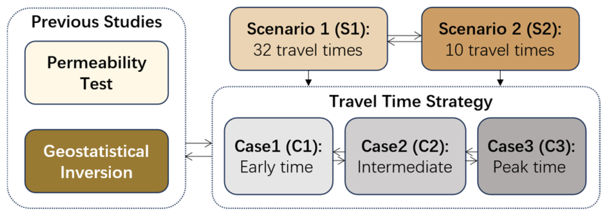
Scenario 1 utilizes all 32 available travel times obtained from the four thermal tracer injection tests, representing a relatively data-rich condition that fully exploits the collected temperature signals. Scenario 2 deliberately reduces the data set to 10 travel times (setting Ports 11, 17, 23, and 29 as observation ports), simulating a sparse-observation situation that is common in field applications where monitoring points are limited. The contrast between these two scenarios allows a direct assessment of how the density of travel–time information affects the resolution and robustness of the reconstructed hydraulic conductivity (K) field. In both scenarios, the inversion assimilated only the scalar travel–time values, the full temperature breakthrough curves were reserved exclusively for forward validation (Section 4.3).
Within each scenario, three alternative travel–time definitions (Cases 1–3) are employed, following the early-time diagnostics concept established by Brauchler et al. (2003) [36] for HT and subsequently extended to thermal tracer tomography by Somogyvári et al. (2016) [17]. Thermal diffusion smooths the raw temperature breakthrough curve, making the purely advective arrival difficult to pick directly.
Following Brauchler et al. (2003) [36] and Somogyvári et al. (2016) [17], an early characteristic time is identified on the rising limb of the first time-derivative of temperature (T′) at a selected fraction α of its peak. This pick is then converted to the equivalent advective breakthrough time via the correction factor fα:
and:
where α is the chosen fraction of the peak T′ value, τα is the relative time (ratio of the early time to the peak time of T′), and fα is the factor that corrects the picked early time to the ideal advective peak time. The three cases are defined as follows:
- Case 1 adopts the early arrival time t10, defined as the time at which the first derivative of temperature (T′) reaches 10% of its maximum value on the rising limb (α = 0.1). This time is multiplied by the corresponding correction factor f10 to obtain the equivalent advective breakthrough time. The 10% threshold targets the fastest components of the thermal signal, which are least affected by thermal diffusion and are expected to be predominantly sensitive to preferential flow paths and high-permeability channels.
- Case 2 uses a later characteristic time t50, defined at 50% of the peak T′ value (α = 0.5), and corrected by the factor f50. Compared to t10, the 50% threshold integrates thermal transport over a larger volume of the aquifer and is expected to reflect bulk transport properties more strongly than localized fast pathways.
- Case 3 employs the peak time of the first temperature derivative, tpeak, defined as the time when T′ reaches its maximum (i.e., the inflection point of the temperature breakthrough curve). This metric corresponds directly to the peak of the derivative and does not require correction via the transformation factor (i.e., fpeak = 1). Compared to the early-time thresholds, tpeak integrates the entire advective–diffusive history of the thermal front and may provide the most robust estimate under well-controlled advection-dominated conditions, albeit with potentially lower sensitivity to highly localized preferential pathways.
Note that identifying tpeak with the advective arrival time assumes advection-dominated transport. In diffusion-dominated regimes, such as very fine-grained sediments or low-gradient field conditions, the T′ peak can be offset from the true advective front. In the present experiment, the moderate-to-high hydraulic conductivities (Table 1) and the imposed gradient (i = 0.1) ensure advection-dominated conditions throughout the sandbox.
These three definitions systematically probe different portions of the thermal breakthrough curve. The early-time metrics t10 and t50 isolate the advancing thermal front at different stages of its propagation, while tpeak captures the bulk advective arrival.
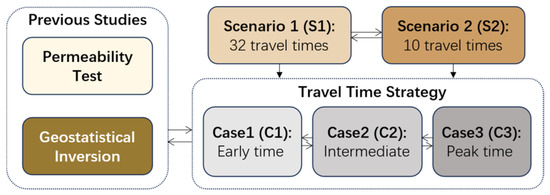
By comparing inversion results derived from these travel-time types under both high (Scenario 1) and low data-volume (Scenario 2) conditions (Figure 2), we aim to: (1) clarify which portion of the thermal signal carries the most valuable information for resolving heterogeneity; (2) determine whether the choice of travel–time definition systematically biases the reconstructed spatial patterns and parameter ranges; and (3) identify the most effective strategy for thermal tracer tomography when applied to limited observational data.
Figure 2.
Workflow of the TTT inversion experiment showing two data-density scenarios and three travel–time definitions.
4. Results and Discussion
The results are organized into three complementary parts that together provide a systematic assessment of the TTT inversion under controlled laboratory conditions.
We first examine the spatiotemporal characteristics of the thermal signals recorded during the four injection tests, presenting temperature contour maps and the extracted travel–time dataset to reveal how thermal breakthrough patterns reflect the known heterogeneous structure of the sandbox aquifer (Section 4.1).
Building on these observations, Section 4.2 evaluates the inversion performance from two perspectives: (1) structural recoverability, such as the ability of different travel–time definitions to reproduce the spatial patterns of the true heterogeneity; and (2) numerical accuracy, meaning how closely the inverted hydraulic conductivity values match the independently measured permeameter benchmarks. The geostatistical inversion result, which assimilated dense steady-state head data, serves as the reference tomogram for this comparison.
Finally, Section 4.3 validates the predictive capability of each inverted conductivity field by using them to forward-model independent thermal tracer tests that were not involved in the inversion, thereby assessing the practical utility of the estimated fields for transport prediction. Throughout, particular attention is paid to the interplay between travel–time definition (Case 1~3) and data density (Scenario 1 vs. Scenario 2), with the aim of identifying an optimal inversion strategy for sparse thermal datasets.
4.1. Thermal Signal Observations
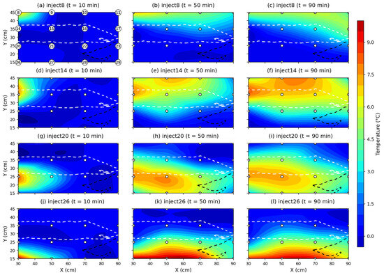
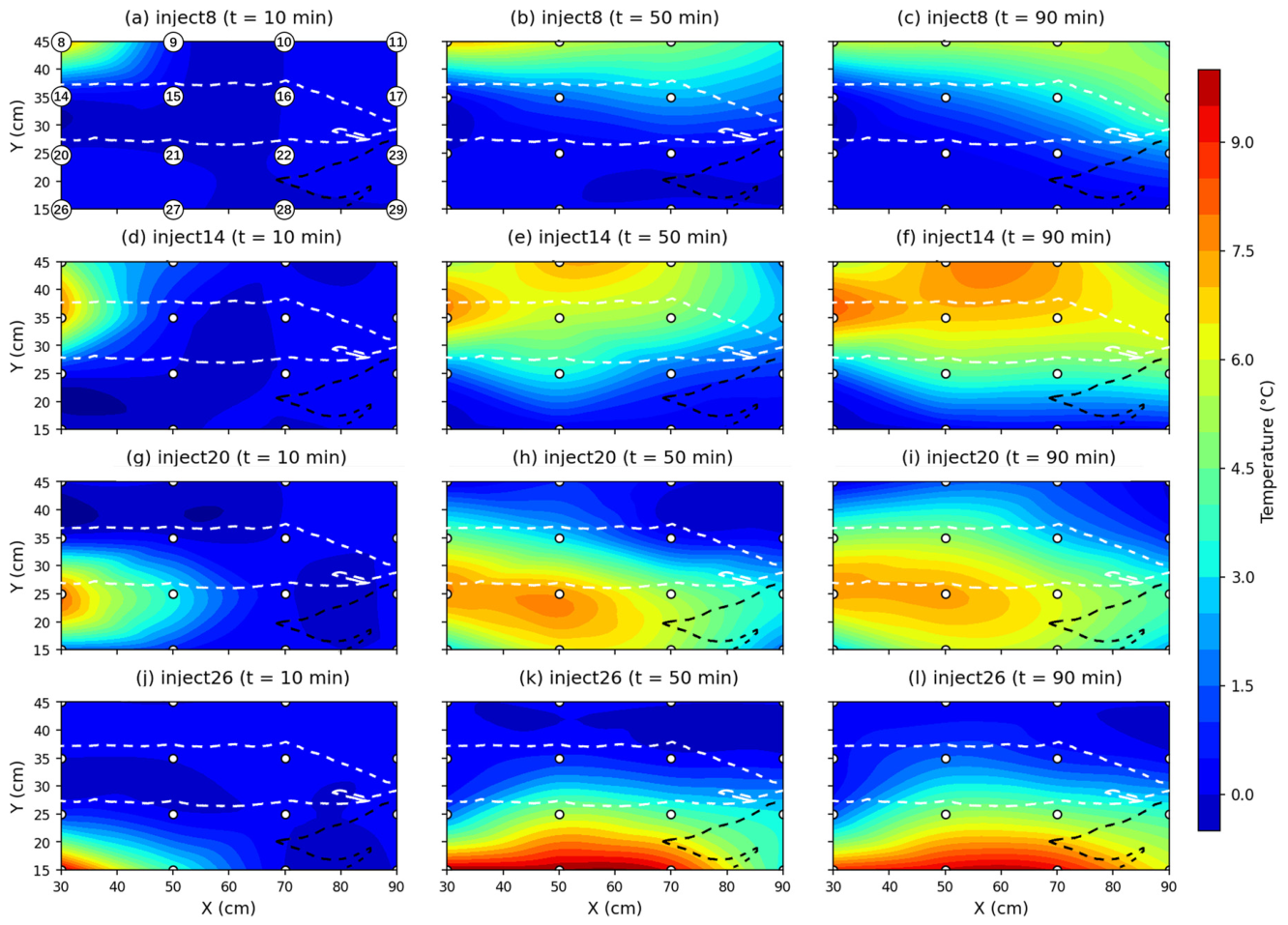
A thermal contour map of the synthetic aquifer (Figure 3) was generated using temperature data collected at the 16 monitoring ports. Figure 3 presents the temperature field at three time points within the sandbox (X: 30–90 cm, Y: 15–45 cm) during the four consecutive thermal tracer injection experiments. Over 16 temperature monitoring ports (arranged in four arrays: Ports 8–11, 14–17, 20–23, and 26–29), the thermal responses induced by heat injections at different locations were captured. Panels in each row correspond to injections at Ports 8 (Figure 3a–c), 14 (Figure 3d–f), 20 (Figure 3g–i), and 26 (Figure 3j–l). Columns indicate the elapsed time since the injection started: t = 10, 50, and 90 min.
Figure 3.
Thermal contour maps of the sandbox (X: 30–90 cm, Y: 15–45 cm) at t = 10, 50, and 90 min during four consecutive thermal tracer injections: (a–c) Port 8; (d–f) Port 14; (g–i) Port 20; (j–l) Port 26. The white and black dotted lines outline the low-permeability Layer 3 and high-permeability Layer 1, respectively.
The thermal transport behavior exhibits a clear dependence on the layered heterogeneity of the sandbox: (1) the low-permeability layer (white dotted line) acts as a barrier to thermal signal propagation; whereas (2) the high-permeability layer (black dotted line) acts as preferential pathways that attract thermal plumes. The apparent “gap” in Figure 3d–f (x = 40–50 cm, y = 38–43 cm) is an interpolation artifact resulting from the limited density of temperature sensors in this region.
As shown in the first column (t = 10 min), the thermal fronts originating from Ports 20 and 26 spread more rapidly in the lateral direction compared to those from Ports 8 and 14, which exhibit a tendency to migrate upward. These observations are consistent with the spatial distribution of hydraulic conductivity in the sandbox. In the second column (t = 50 min), the low-permeability layer near Ports 14, 15, and 16 effectively impedes the vertical propagation of the thermal signal. Meanwhile, the high-permeability layer located around Ports 23 and 29 attracts the thermal plumes injected from Ports 8 and 14, resulting in a downward migration trend after the heat front overcomes the low-permeability barrier.
The high-permeability area located above the monitored temperature area (outside the Y = 45 cm boundary) exerts a significant deflection effect on the thermal signal. Although the sandbox has a finite thickness (10 cm), this dimension is small relative to the lateral extent (120 cm × 60 cm) and the front and back boundaries are impermeable, so the flow field is predominantly two-dimensional in the X–Y monitoring plane. Localized three-dimensional flow components near injection ports cannot be ruled out but are expected to be secondary. The injection temperature rise was +7.3 °C at Ports 8 and 14, +7.8 °C at Port 20, and +9.8 °C at Port 26 (Table 2). However, the maximum temperature rise at the downstream monitoring ports during the Port 8 injection was approximately 5 °C (Ports 9–11), substantially lower than that at downstream ports during the injections at Ports 14 and 20. This suggests that most of the heat injected at Port 8 is diverted through the high-permeability area in the upper-left corner of the sandbox and exits through the right boundary. This high-permeability area was independently identified by geostatistical inversion (Figure 1b). As a result, the thermal response at Ports 9–11 is weaker than expected. Similarly, Figure 3d–f indicate that the thermal tracer injected at Port 14 tends to migrate toward the high-permeability area above the monitored zone, further confirming the preferential flow path induced by the upper high-permeability area.
4.2. Inversion Results
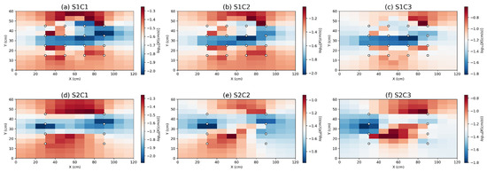
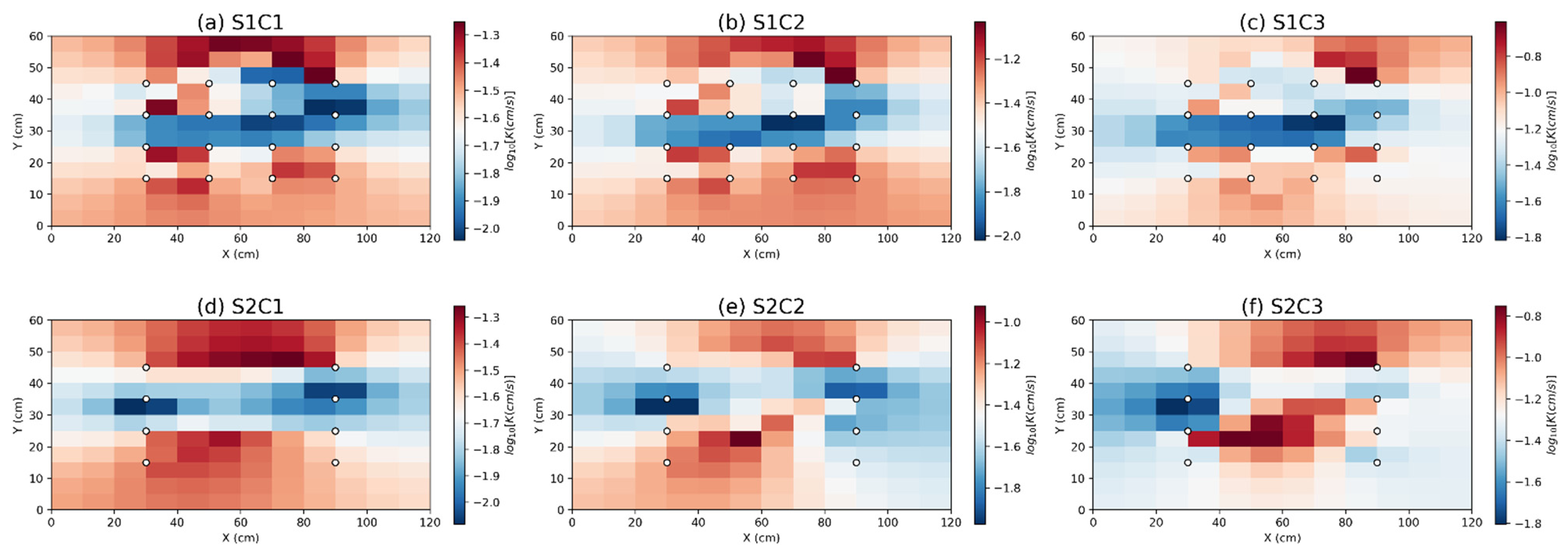
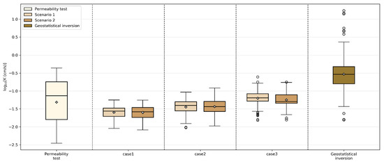
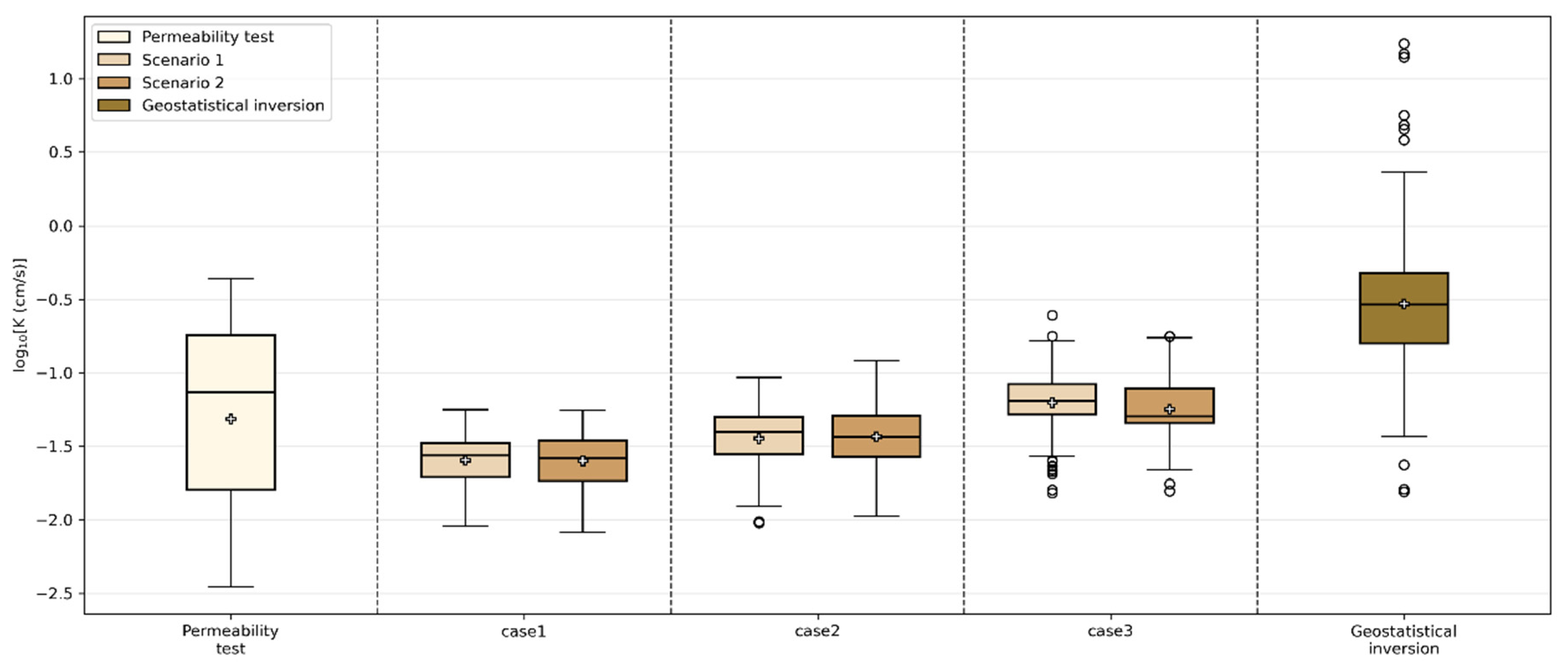
Thermal tracer tomography was performed using travel times obtained from 32 and 10 effective source-receiver combinations for Scenario 1 and Scenario 2, respectively (Table 3). These three travel-time definitions include early-time (t10), mid-time (t50), and peak-time (tpeak). The inversion was performed according to the scenario examples in Table 3, and the inversion results are shown in Figure 4. A box plot of log10 K was also generated based on the inversion results, as shown in Figure 5.
Figure 4.
Inversion results from TTT: (a–c) Scenario 1 (data-rich, n = 32) using Case 1–3; (d–f) Scenario 2 (data-sparse, n = 10) using Case 1–3.
Figure 5.
Boxplot comparison of log10 K distributions from TTT inversion cases (Scenarios 1 and 2), Permeameter Tests, and Geostatistical Inversion.
4.2.1. Structure Estimation Performance
In Scenario 1 (Figure 4a–c), where a sufficient number of travel–time data were available (n = 32), the three different travel–time definitions yielded generally comparable results in capturing the main geological structures and spatial continuity of the sandbox. As shown in Figure 4a–c, the inversions consistently reproduced three distinct zones: (1) Middle low-permeability zone (blue region): All definitions successfully identified this zone. The inversions based on the t50 and tpeak strategies exhibited a closer match to the actual packing design; (2) Top high-permeability zone (red region): All travel time strategies yielded similar performances in identifying this upper zone. However, the t10 and t50 strategies resulted in a slightly higher degree of spatial connectivity than the tpeak strategy; (3) Bottom-right high-permeability zone (red region): All definitions captured the high-permeability layer located near Ports 22 and 23. In addition, a secondary high-permeability area was resolved toward the left side. This may reflect localized hydraulic gradients near the injection ports, where higher flow velocities produce earlier thermal arrivals.
In Scenario 2 (Figure 4d–f), where data were sparse (only 10 travel times from Ports 11, 17, 23, and 29), the early-time t10 inversion proved superior to the t50 and tpeak inversions in preserving the continuity of the geological structure. As shown in Figure 4d, the t10 inversion produced a smoother field compared to Scenario 1 (Figure 4a), but successfully identified the distinct layered low-permeability structure in the middle of the sandbox. In contrast, the t50 (Figure 4e) and tpeak (Figure 4f) inversions failed to reconstruct this layered heterogeneity. Furthermore, the small high-permeability zone in the bottom-right corner was not captured by any of the travel–time definitions in Scenario 2, likely because of the limited spatial coverage and the small size of the target structure.
The contrast in structural recoverability among the three travel–-time definitions can be interpreted within the early-time diagnostics (ETD) framework originally proposed by Somogyvári et al. [17]. In their theoretical development, travel times extracted from the rising limb of the temperature derivative curve, specifically at low α fractions, are least affected by thermal diffusion and thus most faithfully represent the advective component of heat transport. Our experimental results provide direct laboratory evidence supporting this theoretical prediction: the t10 strategy, which targets the earliest detectable fraction of the thermal signal, uniquely preserves structural continuity under sparse monitoring conditions, where t50 and tpeak fail.
The superior structural imaging capability of t10, and its trade-off against transport prediction accuracy, can be understood from the physics of thermal diffusion. Early travel times (t10) are extracted at low α fractions (α = 0.1) on the rising limb of the temperature derivative curve, where the thermal signal has experienced the least cumulative diffusive smoothing. These earliest-arriving components propagate predominantly along the fastest advective pathways, streamline bundles that are narrow and highly sensitive to local K contrasts. Because each t10 value carries information about a spatially localized K feature, the inversion problem remains well-conditioned even with limited ray coverage (Scenario 2). In contrast, t50 and tpeak integrate thermal transport over progressively larger volumes of the aquifer, accumulating diffusive history that smooths away the signatures of sharp K boundaries. When ray coverage is sparse, this diffusive dilution leads to insufficient constraints for resolving fine-scale heterogeneity (as observed in Figure 4e,f). This physical mechanism explains why t10 uniquely preserves structural continuity under sparse monitoring conditions. This structure–accuracy trade-off is a fundamental characteristic of TTT that should inform strategy selection in field applications.
In summary, the comparative inversion results demonstrate a clear trade-off between data density and the robustness of different travel–time definitions for thermal tracer tomography. Under high data density conditions (Scenario 1), all three travel–time definitions provided satisfactory reconstructions, with the t50 and tpeak strategies offering a slightly better match to the known packing structure. However, under sparse data conditions (Scenario 2), the t10 strategy proved significantly more resilient, successfully capturing the primary layered heterogeneity where the t50 and tpeak strategies failed. These findings suggest that early travel times (t10) provide a more robust and reliable choice for characterizing the structural continuity of heterogeneous aquifers when monitoring networks are limited or data sets are incomplete.
4.2.2. Numerical Estimation Accuracy
Figure 5 presents the distribution of logarithmic permeability, log10 K, derived from different inversion methods and travel–time strategies using boxplots. Specifically, the TTT inversion results exhibit significant parameter range compression:
- Case 1 (t10): The inversion results exhibit pronounced low-value clustering. The boxes for both scenarios (Scenario 1 and Scenario 2) concentrate within a narrow range of approximately −2.1 to −1.25. This indicates that inversions utilizing early travel times (t10) yield a relatively low and uniform estimation of permeability with minimal spatial variability.
- Case 2 (t50): Compared to Case 1, the median shifts slightly upward (approximately −1.4), yet the distribution range remains constrained, failing to capture extreme permeability values.
- Case 3 (tpeak): This strategy demonstrates the best performance among the TTT cases. Scenario 1 Case 3 (32 travel times) exhibits a slightly extended upper quartile, with outliers reaching higher values (approximately −0.7). In contrast, Scenario 2 Case 3 (10 travel times) presents a much more compressed distribution.
Within the reference groups: (1) Permeameter test: The median is approximately −1.0, with a broad distribution ranging from −2.5 to −0.4, reflecting the inherent physical heterogeneity of the test domain; (2) Geostatistical inversion: The distribution is skewed substantially toward high values, with a median of approximately −0.5 and extreme outliers above 1.0.
Comparison of the results reveals differences among the inversion strategies. First, all TTT inversions underestimate the absolute permeability, with their medians falling below that of the reference test. Conversely, the geostatistical inversion generally overestimates permeability. Second, within the TTT approaches, we find that the choice of travel–time definition directly impacts the spatial variability of the inversion results. As evident in Figure 5, Case 3 (utilizing peak arrival time) yields greater data variance and more high-value outliers compared to Case 1 (utilizing early arrival time). This suggests that, under the high-gradient conditions of this sandbox, the fα correction (Equation (4)) applied to the early-time picks t10 and t50 produces equivalent travel times (tpeak*) that exceed the directly measured tpeak, leading to more pronounced K compression. The raw early-time picks themselves correspond to the fastest arrival, and the fα correction extrapolates beyond the true advective peak under these conditions. This overcorrection may be related to the simplified one-dimensional advection–diffusion model used to derive fα (Equation (4)), which may not fully capture the multi-path geometry of thermal transport in heterogeneous media.
The systematic underestimation of K ranges by TTT observed in this study converges with findings from several independent investigations. Somogyvári et al. [17] reported slightly underestimated K values in their synthetic numerical experiments, while Somogyvári and Bayer [18] mentioned that their field-inverted K values were consistently lower than those from slug tests. Liu et al. [19] similarly observed that travel–time-based inversion averages K along fracture pathways in fractured rock, suppressing true spatial variability. The recurrence of this pattern across numerical, laboratory, and field scales, and across both porous and fractured media, strongly suggests that the travel–time integration method is the dominant contributor to the observed K underestimation. We note that experimental factors (including temperature sensor precision, injection flow-rate stability, and travel-time picking uncertainty) may also contribute to the observed compression. However, this underestimation pattern recurs across studies with substantially different experimental setups [17,18,19]. This suggests that the primary cause lies in the TTT methodology itself rather than in specific equipment limitations. A definitive separation of methodological and experimental contributions would require a formal uncertainty propagation analysis, which is beyond the scope of the present study.
The physical origin of this systematic K underestimation lies in the travel–time integral formulation (Equation (1)). The inversion solves for the harmonic-mean-like K along each source-receiver ray path, which inherently down-weights high-K channels and compresses the recovered K range toward lower values. As shown in Section 3.1, the simplification of constant ϕ, R, and i contributes minimal additional bias (about ±0.2 log10 K).
Collectively, the results from Figure 5 indicate that TTT provides a relatively stable yet systematically underestimated K field. Compared with geostatistical inversion based on steady-state hydraulic head, TTT exhibits a significant “numerical compression” phenomenon and can be expected to underestimate the migration rate of thermal tracers. This limitation can be partially alleviated by employing the tpeak strategy (Case 3) combined with a larger travel-time dataset (Scenario 1). However, a fundamental resolution likely requires more advanced mitigation strategies, such as incorporating spatially variable hydraulic gradient and porosity fields derived from steady-state head data, applying a post-inversion bias correction, or adopting a joint inversion framework that simultaneously assimilates hydraulic and thermal observations [18,19].
4.3. Forward Validation of Transport Prediction
For validation, the reconstructed 2D K fields were implemented in a numerical forward model using the identical setup as the laboratory experiments. Homogeneous thermal properties were assumed in the forward simulations. Although thermal diffusivity varies with lithology in reality, the same assumption is applied uniformly to all inverted K fields, so the relative ranking of their predictive performance is unaffected. Future studies should explore coupled hydraulic–thermal parameter inversion to improve absolute prediction accuracy.
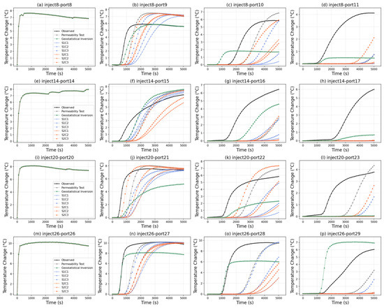
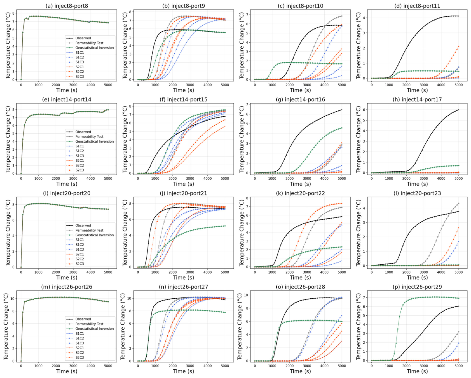
A full tomographic experiment was simulated, incorporating four independent thermal tracer injections (Ports 8, 14, 20, and 26). In the numerical model, the actual recorded time-series temperature data from the laboratory injection ports were applied as the boundary condition, rather than assuming a constant injection temperature. Consequently, the simulated breakthrough curves inherently reflect the minor temperature fluctuations observed at the injection ports (Figure 6a,e,i,m), caused by unavoidable ambient temperature variations during the long-duration experiments. The simulated BTCs were then compared against the observed BTCs from the laboratory data.
Figure 6.
Comparison of observed (black solid line) and simulated thermal breakthrough curves for validation. Each row corresponds to one injection test: (a–d) Port 8; (e–h) Port 14; (i–l) Port 20; (m–p) Port 26.
To evaluate the predictive capability of the inverted fields, the observed thermal responses were compared with simulated responses using fields derived from the Permeameter Test, Geostatistical Inversion, and the cases of two inversion scenarios (S1C1-3 and S2C1-3). The parameter settings of numerical validation are shown in Table 4. The complete data can be obtained from the attachment. Note that the inversion used only the scalar travel times extracted from the BTCs, whereas the validation tests the ability of the inverted K field to reproduce the complete temperature time-series. Although the inversion and validation data originate from the same set of thermal tracer experiments, they are distinct in type (scalar vs. time-series) and serve fundamentally different purposes. The validation therefore constitutes an out-of-sample prediction test, as the time-series information fed into the forward model was excluded from the inversion, with the caveat that a fully independent experimental validation (e.g., using tracer tests not involved in travel–time extraction) was not performed.
Table 4.
Input parameters for numerical forward simulations.
Figure 6 shows that all three model types have inherent limitations in predicting tracer transport. The TTT inversion results are relatively similar to those from the Permeameter Test, as both methods produce comparable estimates of the mean hydraulic conductivity. This leads to a systematic underestimation of the thermal front velocity, with prediction errors increasing as the source-receiver distance grows.
The geostatistical inversion serves as a reference benchmark rather than a directly comparable alternative to TTT. It assimilated 368 steady-state hydraulic head observations, over an order of magnitude more data than the 32 travel times used in TTT Scenario 1, and it therefore provides an upper-bound estimate of the predictive performance achievable with dense hydraulic data for the same aquifer. Details of the geostatistical inversion methodology are provided in Qiu et al. (2025) [33]. A controlled comparison with balanced data volumes would require future work and is beyond the scope of this study.
As expected, all simulated BTCs derived from the TTT inverted fields exhibit a systematic delayed arrival of the thermal signal (quantified in Table 5) relative to the observed data (black solid line). This time-lag behavior is consistent across the four injection events and is particularly pronounced for the TTT inversion based on early-time travel time (S1-2C1), which tends to underestimate the velocity of the thermal front.
Table 5.
Quantitative metrics for thermal transport prediction performance.
To complement the visual comparison, two categories of quantitative performance metrics were computed for each inverted K field (Table 5). Temperature amplitude metrics (RMSE, MAE, and Pearson correlation coefficient r) were calculated over the full BTC time-series at each source–receiver pair. Thermal arrival time errors were derived by extracting travel times from the temperature derivative dT/dt at characteristic thresholds (10%, 50%, and peak) and computing the absolute (abs [s]) and relative (rel [%]) deviation from the observed travel times. For each injection test, the three downstream observation ports were used for performance evaluation (Ports 9–11 for injection at Port 8; Ports 15–17 for injection at Port 14; Ports 21–23 for injection at Port 20; Ports 27–29 for injection at Port 26), yielding a total of 12 source–receiver pairs. The injection port itself was excluded because its temperature serves as the model boundary condition and does not reflect predictive performance. Detailed metrics are provided in the Supplementary Materials.
The quantitative metrics confirm and strengthen the qualitative observations from Figure 6. The geostatistical inversion achieves the highest Pearson correlation (r = 0.89) and the lowest RMSE (2.31 °C) among all methods, with thermal arrival time errors of only 289~589 s (36~41% relative). Among the TTT strategies, tpeak (S1C3 and S2C3) consistently outperforms t50 and t10 on every metric: higher r (0.66~0.69 vs. 0.50~0.55), lower RMSE (2.73~2.79 °C vs. 3.36~3.60 °C), and substantially lower arrival time errors (132~132% vs. 171~228% relative). Scenario 2 (10 travel times) degrades only marginally from Scenario 1 (32 travel times) for all three strategies, confirming that the choice of travel–time definition exerts a stronger influence on predictive performance than data density within the tested range.
An apparent paradox emerges when comparing these predictive metrics (Table 5) with the structural inversion results (Section 4.2.1): t10 best preserves structural continuity under sparse data yet yields the poorest transport predictions. This reveals a fundamental structure–accuracy trade-off in TTT. Early travel times (t10) are the least diffusion-affected portion of the thermal signal and therefore capture the advective structure most faithfully, which explains the superior structural imaging capability of t10. However, the fα correction required to convert early picks to equivalent advective travel times overcompensates under the high-gradient conditions of this sandbox (as discussed in Section 4.2.2), producing systematically overestimated travel times, compressed K ranges, and consequently the largest transport prediction errors. Conversely, tpeak integrates more diffusive history and yields slightly blurred structural images, but its K estimates are less compressed and its transport predictions are substantially more accurate. This trade-off suggests that the optimal TTT strategy depends on the end goal: t10 is preferable for structural characterization in sparse monitoring networks, while tpeak or joint inversion approaches should be favored when transport prediction accuracy is paramount.
The interplay between data density and inversion performance observed here extends previous findings from the same sandbox platform. Qiu et al. (2025) [33] demonstrated that enriching a hydraulic head dataset with tracer injection data (from 184 to 272 measurements) significantly improved solute transport predictions from HT-based K fields. Zhao et al. (2022) [32] showed that reducing calibration data from eight to four pumping tests degraded HT performance, though accurate geological prior information could partially compensate. Our results complement these findings from the thermal tracer perspective: while data density clearly affects TTT performance, the choice of travel–time definition provides an additional degree of freedom; the early-time t10 strategy effectively compensates for reduced data volume, functioning analogously to the geological prior information in Zhao et al.’s (2022) [32] HT analysis. This suggests that in field scenarios where dense monitoring networks are impractical, the combination of optimal travel–time diagnostics with sparse but strategically placed sensors may offer a viable characterization strategy.
Nevertheless, despite these relative differences, all inversion methods based on a single data source exhibit significant limitations when predicting tracer transport in heterogeneous aquifers. This indicates that relying on a single type of observation (either thermal travel times or steady-state heads) is insufficient to fully characterize the complex transport behavior.
4.4. Limitations
Several limitations of this study should be noted. The sensitivity of inversion results to porosity, hydraulic gradient, and thermal retardation factor was assessed via first-order error propagation from Equations (1) and (2) (Section 3.1), indicating a combined uncertainty of approximately ±0.2 log10 K, substantially smaller than the observed K compression (approximately 1.0 log10 K). The effect of data density was explicitly examined through comparison of Scenario 1 and Scenario 2 (32 vs. 10 travel times; Figure 4).
Two additional factors that may influence the results were not systematically quantified in this study. First, the spatial arrangement, total number, and selection of the 16 monitoring ports directly determine which regions of the aquifer are sampled by thermal rays, potentially affecting both the resolved structures and the degree of K compression. The finding that t10 outperforms t50 and tpeak under sparse monitoring (Scenario 2) is specific to the four-port layout (Ports 11, 17, 23, and 29) tested here; alternative sensor layouts could yield different rankings of travel–time definitions. Second, measurement noise includes temperature sensor precision (0.1 °C), injection flow-rate fluctuations, and the uncertainty inherent in picking travel times from smoothed BTCs. These noise sources propagate into the inversion and may amplify the K compression. Controlled noise injection tests and systematic comparison of alternative sensor layouts would be valuable for future work to further constrain these contributions.
5. Conclusions
This study presents a controlled laboratory sandbox investigation to evaluate the efficacy of TTT for characterizing aquifer heterogeneity. Thermal injection experiments were conducted in a 2D heterogeneous aquifer with known hydraulic conductivity distributions, and arrival times were extracted using three distinct travel–time definitions (t10, t50, and tpeak) under both data-rich (32 travel times) and data-sparse (10 travel times) conditions. The resultant TTT inversion fields were benchmarked against permeameter tests and a geostatistical inversion that assimilated dense steady-state head data, with the performance assessed in terms of structural recoverability, parameter range recovery, and forward-prediction capability. The key findings are summarized as follows:
- Under abundant observational data, all three travel–time definitions satisfactorily reproduce the primary layered heterogeneity of the sandbox, with the t50 and tpeak providing marginally better fidelity to the true low-permeability interlayer. Crucially, when the data volume is severely reduced, only the t10 preserves the spatial continuity of the dominant heterogeneity patterns, demonstrating its superior robustness for structural identification in sparse monitoring networks.
- All TTT inversion results exhibit pronounced compression of the inverted K range, with median values systematically lower than those obtained from permeameter tests. This numerical compression causes a low-value clustering that substantially suppresses spatial variability. In contrast, the geostatistical inversion overestimates absolute conductivity and generates spurious high-value extremes. Among the TTT schemes, the tpeak strategy combined with a larger travel-time dataset partially alleviates the range compression, yielding slightly greater variance and a shift towards higher values.
- Forward simulations using the inverted K fields reveal that all TTT-based models systematically delay the arrival of thermal breakthrough curves (Table 5), with the discrepancy increasing with source–receiver distance. Quantitative performance metrics confirm that among TTT strategies, tpeak achieves the best transport predictions (r = 0.66~0.69), while t10, despite superior structural imaging under sparse data, yields the largest prediction errors because of fα overcorrection. Although the geostatistical inversion, benefiting from abundant hydraulic head data, reproduces some late-time tailing and breakthrough truncation features more accurately, it still fails to fully capture the observed thermal transport behavior. These results collectively demonstrate that neither thermal travel times nor steady-state heads alone are sufficient to fully resolve the subsurface flow and transport properties.
- The complementary biases revealed in this study strongly motivate a joint hydraulic–thermal inversion framework. Specifically, TTT underestimates K but preserves structural connectivity, particularly via early-time diagnostics, while geostatistical inversion overestimates K with spurious extremes. Conceptually, thermal travel times would constrain the spatial pattern of heterogeneity, steady-state head data would anchor the absolute K magnitude, and temperature time-series would calibrate transport parameters. Liu et al. (2022) [19] and Somogyvári and Bayer (2017) [18] reached the same conclusion, and our experimental results provide the first controlled laboratory evidence quantifying the complementary biases that such a framework must reconcile. Future sandbox and field investigations should prioritize the development of computationally efficient joint inversion algorithms capable of assimilating transient hydraulic and thermal signals concurrently.
Overall, this work provides the first controlled experimental evidence quantifying how travel-time selection and data volume govern the performance of thermal tracer tomography at the laboratory scale. The findings highlight that although early-time diagnostics offer a robust pathway for structural imaging under sparse data, accurate quantification of parameter ranges and reliable transport prediction demand the fusion of multiple hydrogeological data streams.
Supplementary Materials
The following supporting information can be downloaded at: https://www.mdpi.com/article/10.3390/w18131543/s1, Supplementary_Material_s1: Table S1. Permeameter test results; Figures S1–S12. Thermal tracer tomography results at ports 8, 14, 20, and 26, including temperature breakthrough curves (e.g., S1, S3, S5, and S7), derivative curves (e.g., S2, S4, S6, and S8), and validation results (e.g., S9–S12). Supplementary_Material_s2: Observed thermal data, steady hydraulic head for geostatistical inversion, and detailed metrics.
Author Contributions
Data curation, Y.S. and L.F.; Formal analysis, H.Q. and Y.S.; Methodology, R.H., H.Q. and Y.S.; Software, Y.S.; Supervision, R.H.; Writing—original draft, H.Q. and Y.S.; Writing—review and editing, H.Q., R.H. and Y.S. All authors have read and agreed to the published version of the manuscript.
Funding
This research was funded by the National Natural Science Foundation of China (NSFC Grant No. 42372280), “Investigating the permeability loss and the spatial heterogeneous permeability change of zero-valent iron permeable reactive barrier for groundwater remediation”.
Data Availability Statement
The original contributions presented in this study are included in the article and Supplementary Materials. Further inquiries can be directed to the corresponding author.
Acknowledgments
During the preparation of this manuscript, the authors used DeepSeek V4 Pro for the purposes of text checking. The authors have reviewed and edited the output and take full responsibility for the content of this publication.
Conflicts of Interest
The authors declare no conflicts of interest.
Abbreviations
The following abbreviations are used in this manuscript:
| TTT | travel-time-based Thermal Tracer Tomography |
| HT | Hydraulic Tomography |
| DTS | Distributed Temperature Sensing |
| BTCs | Breakthrough Curves |
References
- Bear, J. Dynamics of Fluids in Porous Media; Dynamics of Fluids in Porous Media; American Elsevier Publishing Company: Amsterdam, The Netherlands, 1972; ISBN 978-0-444-00114-6. [Google Scholar]
- Dagan, G. Flow and Transport in Porous Formations; Springer: Berlin/Heidelberg, Germany; New York, NY, USA, 1989; ISBN 978-0-387-51602-8. [Google Scholar]
- Zheng, C.; Gorelick, S.M. Analysis of Solute Transport in Flow Fields Influenced by Preferential Flowpaths at the Decimeter Scale. Groundwater 2003, 41, 142–155. [Google Scholar] [CrossRef] [Scilit] [PubMed]
- Vasco, D.W.; Keers, H.; Karasaki, K. Estimation of Reservoir Properties Using Transient Pressure Data: An Asymptotic Approach. Water Resour. Res. 2000, 36, 3447–3465. [Google Scholar] [CrossRef] [Scilit]
- Brauchler, R.; Cheng, J.-T.; Dietrich, P.; Everett, M.; Johnson, B.; Liedl, R.; Sauter, M. An Inversion Strategy for Hydraulic Tomography: Coupling Travel Time and Amplitude Inversion. J. Hydrol. 2007, 345, 184–198. [Google Scholar] [CrossRef] [Scilit]
- Brauchler, R.; Hu, R.; Hu, L.; Jiménez, S.; Bayer, P.; Dietrich, P.; Ptak, T. Rapid Field Application of Hydraulic Tomography for Resolving Aquifer Heterogeneity in Unconsolidated Sediments. Water Resour. Res. 2013, 49, 2013–2024. [Google Scholar] [CrossRef] [Scilit]
- Vasco, D.W. An Extended Trajectory Mechanics Approach for Calculating the Path of a Pressure Transient: Derivation and Illustration. Water Resour. Res. 2018, 54, 2642–2660. [Google Scholar] [CrossRef] [Scilit]
- Vasco, D.W.; Doetsch, J.; Brauchler, R. An Extended Trajectory-Mechanics Approach for Calculating the Path of a Pressure Transient: Travel-Time Tomography. Hydrol. Earth Syst. Sci. 2019, 23, 4541–4560. [Google Scholar] [CrossRef] [Scilit]
- Vasco, D.W.; Datta-Gupta, A. Asymptotic Solutions for Solute Transport: A Formalism for Tracer Tomography. Water Resour. Res. 1999, 35, 1–16. [Google Scholar] [CrossRef] [Scilit]
- Illman, W.A.; Berg, S.J.; Yeh, T.-C.J. Comparison of Approaches for Predicting Solute Transport: Sandbox Experiments. Groundwater 2012, 50, 421–431. [Google Scholar] [CrossRef] [Scilit] [PubMed]
- Brauchler, R.; Böhm, G.; Leven, C.; Dietrich, P.; Sauter, M. A Laboratory Study of Tracer Tomography. Hydrogeol. J. 2013, 21, 1265–1274. [Google Scholar] [CrossRef] [Scilit]
- Saar, M.O. Review: Geothermal Heat as a Tracer of Large-Scale Groundwater Flow and as a Means to Determine Permeability Fields. Hydrogeol. J. 2011, 19, 31–52. [Google Scholar] [CrossRef] [Scilit]
- Leaf, A.T.; Hart, D.J.; Bahr, J.M. Active Thermal Tracer Tests for Improved Hydrostratigraphic Characterization. Groundwater 2012, 50, 726–735. [Google Scholar] [CrossRef] [Scilit] [PubMed]
- Rau, G.C.; Andersen, M.S.; McCallum, A.M.; Roshan, H.; Acworth, R.I. Heat as a Tracer to Quantify Water Flow in Near-Surface Sediments. Earth-Sci. Rev. 2014, 129, 40–58. [Google Scholar] [CrossRef] [Scilit]
- Bakker, M.; Caljé, R.; Schaars, F.; van der Made, K.-J.; de Haas, S. An Active Heat Tracer Experiment to Determine Groundwater Velocities Using Fiber Optic Cables Installed with Direct Push Equipment. Water Resour. Res. 2015, 51, 2760–2772. [Google Scholar] [CrossRef] [Scilit]
- Doro, K.O.; Cirpka, O.A.; Leven, C. Tracer Tomography: Design Concepts and Field Experiments Using Heat as a Tracer. Groundwater 2015, 53, 139–148. [Google Scholar] [CrossRef] [Scilit] [PubMed]
- Somogyvári, M.; Bayer, P.; Brauchler, R. Travel-Time-Based Thermal Tracer Tomography. Hydrol. Earth Syst. Sci. 2016, 20, 1885–1901. [Google Scholar] [CrossRef] [Scilit]
- Somogyvári, M.; Bayer, P. Field Validation of Thermal Tracer Tomography for Reconstruction of Aquifer Heterogeneity. Water Resour. Res. 2017, 53, 5070–5084. [Google Scholar] [CrossRef] [Scilit]
- Liu, Q.; Hu, R.; Hu, L.; Xing, Y.; Qiu, P.; Yang, H.; Fischer, S.; Ptak, T. Investigation of Hydraulic Properties in Fractured Aquifers Using Cross-Well Travel-Time Based Thermal Tracer Tomography: Numerical and Field Experiments. J. Hydrol. 2022, 609, 127751. [Google Scholar] [CrossRef] [Scilit]
- Song, Y.; Hu, R.; Liu, Q.; Qiu, H.; Hou, X.; Qi, J.; Konadu-Amoah, B. Comparison of Hydraulic Travel Time and Attenuation Inversions, Thermal Tracer Tomography and Geostatistical Inversion for Aquifer Characterization: A Numerical Study. Water 2023, 15, 2401. [Google Scholar] [CrossRef] [Scilit]
- Yeh, T.-C.J.; Liu, S. Hydraulic Tomography: Development of a New Aquifer Test Method. Water Resour. Res. 2000, 36, 2095–2105. [Google Scholar] [CrossRef] [Scilit]
- Zhu, J.; Yeh, T.-C.J. Characterization of Aquifer Heterogeneity Using Transient Hydraulic Tomography. Water Resour. Res. 2005, 41, W07028. [Google Scholar] [CrossRef] [Scilit]
- Zhu, J.; Yeh, T.-C.J. Analysis of Hydraulic Tomography Using Temporal Moments of Drawdown Recovery Data. Water Resour. Res. 2006, 42, W02403. [Google Scholar] [CrossRef] [Scilit]
- Illman, W.A.; Zhu, J.; Craig, A.J.; Yin, D. Comparison of Aquifer Characterization Approaches through Steady State Groundwater Model Validation: A Controlled Laboratory Sandbox Study. Water Resour. Res. 2010, 46, W04502. [Google Scholar] [CrossRef] [Scilit]
- Schwede, R.L.; Li, W.; Leven, C.; Cirpka, O.A. Three-Dimensional Geostatistical Inversion of Synthetic Tomographic Pumping and Heat-Tracer Tests in a Nested-Cell Setup. Adv. Water Resour. 2014, 63, 77–90. [Google Scholar] [CrossRef] [Scilit]
- Berg, S.J.; Illman, W.A. Comparison of Hydraulic Tomography with Traditional Methods at a Highly Heterogeneous Site. Groundwater 2015, 53, 71–89. [Google Scholar] [CrossRef] [Scilit] [PubMed]
- Luo, N.; Zhao, Z.; Illman, W.A.; Berg, S.J. Comparative Study of Transient Hydraulic Tomography with Varying Parameterizations and Zonations: Laboratory Sandbox Investigation. J. Hydrol. 2017, 554, 758–779. [Google Scholar] [CrossRef] [Scilit]
- Qiu, H.; Hu, R.; Luo, N.; Illman, W.A.; Hou, X. Comparison of Travel-Time and Geostatistical Inversion Approaches for Hydraulic Tomography: Synthetic Modeling Study on Data Density and Well Configuration Issues. J. Hydrol. 2023, 618, 129247. [Google Scholar] [CrossRef] [Scilit]
- Sarris, T.S.; Close, M.; Abraham, P. Using Solute and Heat Tracers for Aquifer Characterization in a Strongly Heterogeneous Alluvial Aquifer. J. Hydrol. 2018, 558, 55–71. [Google Scholar] [CrossRef] [Scilit]
- Pouladi, B.; Bour, O.; Longuevergne, L.; de La Bernardie, J.; Simon, N. Modelling Borehole Flows from Distributed Temperature Sensing Data to Monitor Groundwater Dynamics in Fractured Media. J. Hydrol. 2021, 598, 126450. [Google Scholar] [CrossRef] [Scilit]
- Römhild, L.; Ringel, L.M.; Liu, Q.; Hu, L.; Ptak, T.; Bayer, P. Hybrid Discrete Fracture Network Inversion of Hydraulic Tomography Data From a Fractured-Porous Field Site. Water Resour. Res. 2024, 60, e2023WR036035. [Google Scholar] [CrossRef] [Scilit]
- Zhao, Z.; Berg, S.J.; Illman, W.A.; Qi, Y. Improving Predictions of Solute Transport in a Laboratory Sandbox Aquifer through High-Resolution Characterization with Hydraulic Tomography. J. Hydrol. 2022, 615, 128673. [Google Scholar] [CrossRef] [Scilit]
- Qiu, H.; Zhang, J.; Zhang, Y.; Song, Y.; Li, T.; Amoah, B.K.; Hu, R.; Huang, Y. Comparative Predictions of Solute Transport with Hydraulic Tomography in a Laboratory Sandbox Aquifer: The Importance of the Injection Data. Adv. Water Resour. 2025, 206, 105150. [Google Scholar] [CrossRef] [Scilit]
- Somogyvári, M.; Kühn, M.; Reich, S. Reservoir-Scale Transdimensional Fracture Network Inversion. Adv. Geosci. 2019, 49, 207–214. [Google Scholar] [CrossRef] [Scilit]
- Rücker, C.; Günther, T.; Wagner, F.M. pyGIMLi: An Open-Source Library for Modelling and Inversion in Geophysics. Comput. Geosci. 2017, 109, 106–123. [Google Scholar] [CrossRef] [Scilit]
- Brauchler, R.; Liedl, R.; Dietrich, P. A Travel Time Based Hydraulic Tomographic Approach. Water Resour. Res. 2003, 39, 1370. [Google Scholar] [CrossRef] [Scilit]

Disclaimer/Publisher’s Note: The statements, opinions and data contained in all publications are solely those of the individual author(s) and contributor(s) and not of MDPI and/or the editor(s). MDPI and/or the editor(s) disclaim responsibility for any injury to people or property resulting from any ideas, methods, instructions or products referred to in the content. |
© 2026 by the authors. Licensee MDPI, Basel, Switzerland. This article is an open access article distributed under the terms and conditions of the Creative Commons Attribution (CC BY) license.