


Abstract
Some countries grapple with data scarcity for calibration purposes when establishing current hydrodynamic models, which often require many parameters. In this context, this research presents a practical simulation methodology for hydrodynamic modelling suitable for application in bay and estuarine systems based on mass and momentum equations and requiring only one parameter for calibration—bed friction. The proposed simulation methodology is applied to a linear open channel measuring 200,000 m long. A sensitivity analysis of the bed friction is conducted to assess the proposed methodology’s response to the maximum water levels achieved. The results are compared to linear theory, indicating that the proposed simulation methodology effectively represents the water phase. In all simulations, the maximum root mean square error is less than 2.1% when neglecting bed friction and 4.69% when a bed friction of 0.005 is considered. The proposed simulation methodology can be a practical tool for hydrodynamic modelling in shallow waters.
1. Introduction
In recent decades, hydrodynamic modelling has gained significant attention from engineers and researchers, driven by advances in computational techniques and their applications to tidal, coastal, and river interactions for addressing practical challenges [1,2,3]. Early computational models were designed to examine long-period and ordinary tidal-wave propagation through the finite difference method as a numerical integration technique [4,5].
Initially, two-dimensional hydrodynamic models were proposed, with subsequent developments incorporating water quality models that integrated hydrodynamic components. As computational power increased, hydrodynamic models evolved, incorporating more sophisticated theoretical approaches. Quasi-three-dimensional models, such as multilayer models, emerged alongside new numerical solutions like finite difference and finite element methods [6,7]. Additionally, three-dimensional models were developed [8].
With the advancement of modelling techniques such as finite elements, numerical stability issues became apparent, related to the shape of discretisation elements and interpolation functions at boundary conditions [9]. These challenges prompted improvements in discretisation techniques and a renewed focus on accurately representing boundary conditions using curvilinear coordinate systems.
Field data and numerical integration have been used to analyse tidal propagation into estuaries through channels, highlighting significant attenuation due to friction effects and the asymmetrical nature of tides entering estuarine systems [10,11,12]. Studies also examined the changes in tides due to channel constriction between the sea and a lagoon and the impact of bed friction [13,14]. The role of viscosity (eddy effects), bottom topography, wind-generated waves, and their interactions in shallow bay circulation has been investigated using a three-dimensional hydrodynamic model of an idealised estuary with a continuous vertical current profile [15].
Tidal-wave propagation in channels has been explored, such as, for example, on the Gran Canaria Island shelf [16]. This study examined the effects of friction on tidal-wave propagation and the influence of introducing a stationary current at the channel entrance. Numerical experiments utilised explicit finite-difference schemes along a one-dimensional channel of constant depth. Analytical solutions for Kelvin waves in rectangular channels with linearly and exponentially varying depths were also proposed and compared with numerical solutions [17]. The communication between the sea and shallow water bodies through narrow connections has been examined from various perspectives using different models. A three-dimensional hydrodynamic model was used for the numerical analysis of a stratified estuary connected to the sea by a narrow mixed channel [18]. The effect of specific tidal constituents and their relationship with the bed-friction factor using a numerical model applied to the Bristol Channel has been explored [19]. Their findings indicated that the bed-friction coefficient produced contradictory results when calibrating both primary tidal constituents and nonlinear components.
Three-dimensional hydrodynamic finite difference models have been developed for homogeneous and stratified marine regions, employing energy-based models [20]. Advancements in the study of bottom drag coefficients have been made using Doppler current metres. Field data have demonstrated that drag coefficients vary with depth, exhibiting higher values in shallow waters and lower values in deeper waters, where reductions in drag coefficients correlate with increases in the water depth-to-bottom roughness ratio [21].
The Danish Hydraulic Institute (DHI) has developed the MIKE 21 software package over the past few decades for the hydrodynamic modelling of estuaries, bays, and coastal areas [22,23,24]. With hundreds of reported applications worldwide, this software comprises 13 modules applied to four specific areas: Coastal Oceanography and Hydraulics, Environmental Hydraulics, Wave Dynamics, and Coastal Sediment Processes. The hydrodynamic module (HD) is a numerical model for simulating levels and flows in estuaries, bays, and coastal zones, modelling two-dimensional unsteady flow in a vertically homogeneous layer.
As hydrodynamic models have advanced, so has their complexity, the number of parameters they employ, and the quantity and quality of data required for calibration. While these models have been applied globally, where field data are available for calibration, some countries often lack systematic data collection over time and space, hindering the calibration of models with numerous parameters. Consequently, model outcomes frequently depend on the expert judgement of engineers and researchers when selecting calibration parameters.
This research proposes a new simulation methodology for estuaries and bays designed to simplify and reduce calibration costs, making it more appealing from an engineering perspective. This is particularly relevant when evaluating projects at the technical, economic, and social pre-feasibility stages, where assessments are conducted at a macroscopic level with similar precision. The primary objective for government entities is to identify the most probable path to success, optimising the allocation and planning of necessary actions and resources for managing water bodies. The formulation of this methodology is based on the Eulerian equations of mass and momentum conservation, with the proposed methodology focusing on horizontal and surface flows. It incorporates the concept of hydraulic radius for bottom friction, commonly used in channel hydraulics, to account for the effects of lateral wall friction in channels with a narrow width relative to their depth. This simulation methodology aims to provide a simple, versatile, and easily calibratable tool for decision making in planning hydraulic engineering projects that interact with environmentally sensitive water bodies.
The proposed simulation methodology employs a finite-difference discretisation approach. Its innovation lies in proposing a method to calculate water levels at successive wave positions, simplifying the final calculation matrix and enabling rapid convergence.
The novel aspect is estimating water levels at each discretised domain element, a critical factor for adequately operating the proposed methodology in this research. To compute each coefficient in the solution matrix, it is necessary to understand the variation in the water surface level across space (in the X and Y directions). This estimation is grounded in the theory of long-wave velocities in shallow waters, as described by Dean and Dalrymple (1991) [25]. These velocities may be amplified or attenuated due to energy concentration, energy dissipation, bottom friction, and/or lateral wall effects. The proposed procedure estimates the wave’s travel time from the boundary condition (e.g., tide level) to each element and its four sides. It is assumed that the water level at each side of a component is equal to the boundary condition level at time , where is the wave travel time, modified by damping, dissipation, and/or amplification coefficients. The functions used to estimate water levels can be analytical functions derived from linear theory or parametric functions obtained from field data.
This research is structured into the following sections: (i) Materials and Methods, which outlines the simulation methodology used for modelling hydrodynamics in bays and estuarine systems; (ii) Results, where a practical application of the simulation methodology is demonstrated for a rectangular channel measuring 200,000 m in length; and (iii) Discussion, in which a comparison is made between the proposed simulation methodology and linear theory.
2. Materials and Methods
This section presents the proposed simulation methodology developed in this research. It is particularly suited for use in some countries where field data are scarce [25,26,27,28].
2.1. Assumptions
The development of the proposed simulation methodology is based on the following assumptions [5,25,29,30,31]:
- Water density is assumed to be constant.
- No stratification is present.
- The fluid is incompressible.
- The Eulerian equations for the conservation of mass and momentum are valid for non-viscous fluids.
- The theory of long waves in shallow water is applicable.
- The ocean bottom is considered waterproof.
- The driving forces of movement include tides, winds, surface runoff, inputs, and outputs through channels and conduits, and the effect of the Earth’s rotation (Coriolis).
- The dissipative forces of movement include bottom friction, friction with lateral walls, and local losses due to hydraulic structures (bridges, gates, etc.).
2.2. Governing Equations
Considering the Eulerian equations for the conservation of momentum (for an ideal fluid, under a variable regime, with gravity as the only external force) and the conservation law of mass, then:
The general form of the momentum conservation equation can be expressed in terms of its , , and components as follows:
Equation (1a–c) present the theoretical equations for an ideal fluid. Subsequently, friction factors and other inflow and outflow terms are incorporated for real-world conditions.
The principle of the mass conservation equation was applied to account for the fact that mass is neither created nor destroyed within the fluid, as follows:
where , and are water velocities in the , , and , respectively; = water density, and = gravitational acceleration.
For an incompressible flow (), the mass conservation equation (Equation (2)) is transformed to:
The methodology is valid for long waves in shallow waters. For a progressive long wave [25]:
where = wave celerity, = wave height, = wave number , = frequency, = mean water depth, and = time.
Considering that (see Appendix A), then the magnitude of the first-order term in is much greater compared to the advective term in . The momentum equation in direction can be expressed by Equation (6a). Similarly, for the and directions, the momentum equations are given by Equation (6b,c).
The integration of the mass conservation equation can be expressed in terms of the mean horizontal velocities , , and the surface vertical velocity as follows (see Appendix B):
where = initial depth, and = water level.
Momentum and mass equations are expressed in terms of the mean velocities , , the surface variation, the Coriolis parameter () [5], the hydraulic radius (relationship between area and perimeter) as characteristic length, the Chezy resistance coefficient (), and other external forces like wind and barometric pressure represented by and . The Coriolis force is described as an external force; however, in some cases, particularly near the equator, its magnitude becomes negligible. For this theoretical test analysis, it was not considered. Furthermore, its practical implications in everyday engineering applications are often minimal due to the small scale involved. The following expressions are obtained [31]:
where = hydraulic radius.
The initial equations are formulated as the inviscid Euler equations, considering an ideal fluid. Viscosity and other losses are not considered, as real shallow water problems incorporate parameters encompassing theoretical simplifications and are subject to calibration using field data. The effect of bed and wall friction is included because it has the most significant localised impact on water levels and allows, in practice, for all the simplifications made to be accounted for through calibration with field data.
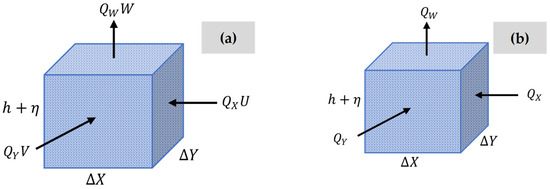
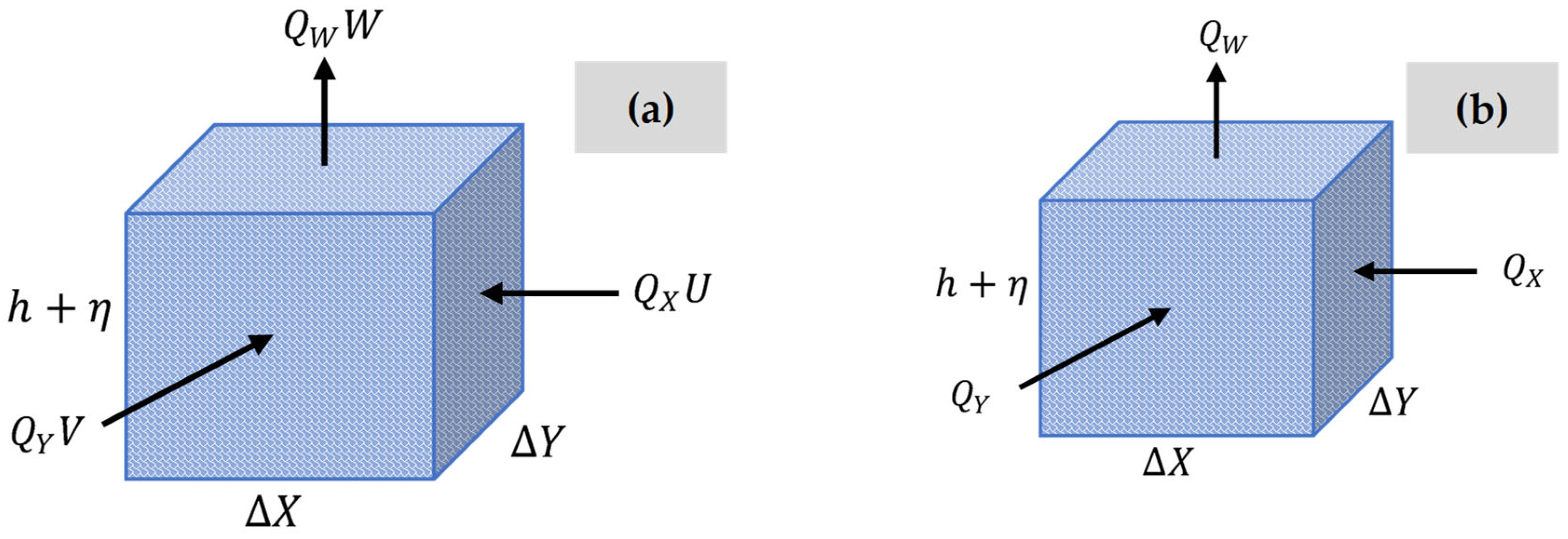
The momentum and mass conservation equations are described as a function of flow rate for an element considering a rectangular parallelepiped with dimensions , , and , as shown in Figure 1.
Figure 1.
Analysis of an element: (a) flows and velocity direction; and (b) diagram of flows.
Multiplying both sides of the momentum equation in the direction by , and considering , and , then:
The term incorporates additional external forces [5,32], encompassing the effects of wind and barometric pressure. It represents a simplified variable that accounts for a finite set of external forces. Despite this simplification, the core concept remains consistent. Wind is typically considered the most significant among these forces due to its pronounced influence on system dynamics.
The following notation was adopted as follows: = flow in the axis direction = , = flow in the axis direction = , = flow in the direction = , water surface level at time in the direction, = water surface level at time , and .
Then, it is possible to demonstrate that:
where and
The hydraulic radius in Equation (10) is presented in a general form. When the equation is transformed to express it in terms of flow rates, it is more specifically denoted as , to emphasise that it corresponds to the -direction.
Considering the definition of , then Equation (11) is expressed as:
Equation (12) is formulated for a discrete element with dimensions , , and . It accounts for variations in flow rate and velocities in the and directions, which are predominantly driven by changes in water level and external forces such as bottom friction, the Coriolis force, and additional influences like wind.
2.3. Numerical Resolution
This section shows the numerical resolution for the simplified hydrodynamic model for estuaries and bays. The terms , , and were used.
The first-order partial derivatives are computed as , , and . Using the finite-difference approximation applied to the variables , Equation (12) is then transformed into:
Rearranging the terms at and , Equation (14) is obtained for the flow in the direction:
Equation (15) is obtained by applying a similar procedure to the momentum equation for the direction:
The mass conservation equation is transformed into a function of the flows in the directions (see Figure 1b).
The finite-difference approximation for the mass conservation law can be expressed as:
However, , , and ; then, the mass conservation equation transforms into:
In this case, the first-order partial derivatives were considered as and . Substituting the finite-difference approximation for the partial derivatives of and with respect to and , using the forward difference method, the following equations are then obtained:
Equation (18) can be extended for time , obtaining:
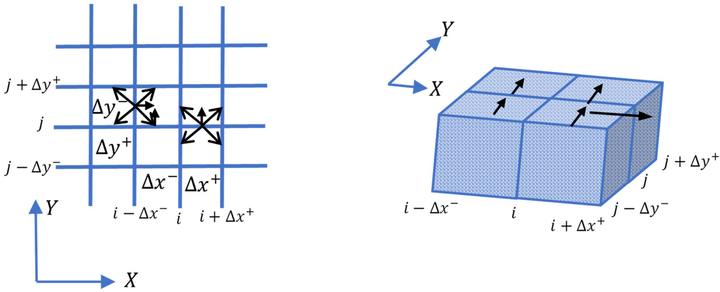
The following notation is defined for the discretisation of the equations in the and domains, where is the flow in the direction, in column , forward of at time , and is the flow in the direction, in row , forward of , as shown in Figure 2 [31].
Figure 2.
Discretisation diagram.
In summary, the momentum equations in and , and the mass conservation equation centred on elements and , are expressed as follows:
where .
The continuity equation is arranged term by term to the momentum equations, resulting in two equations in this research.
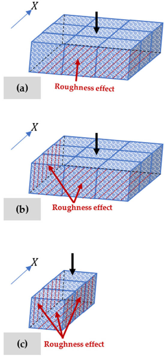
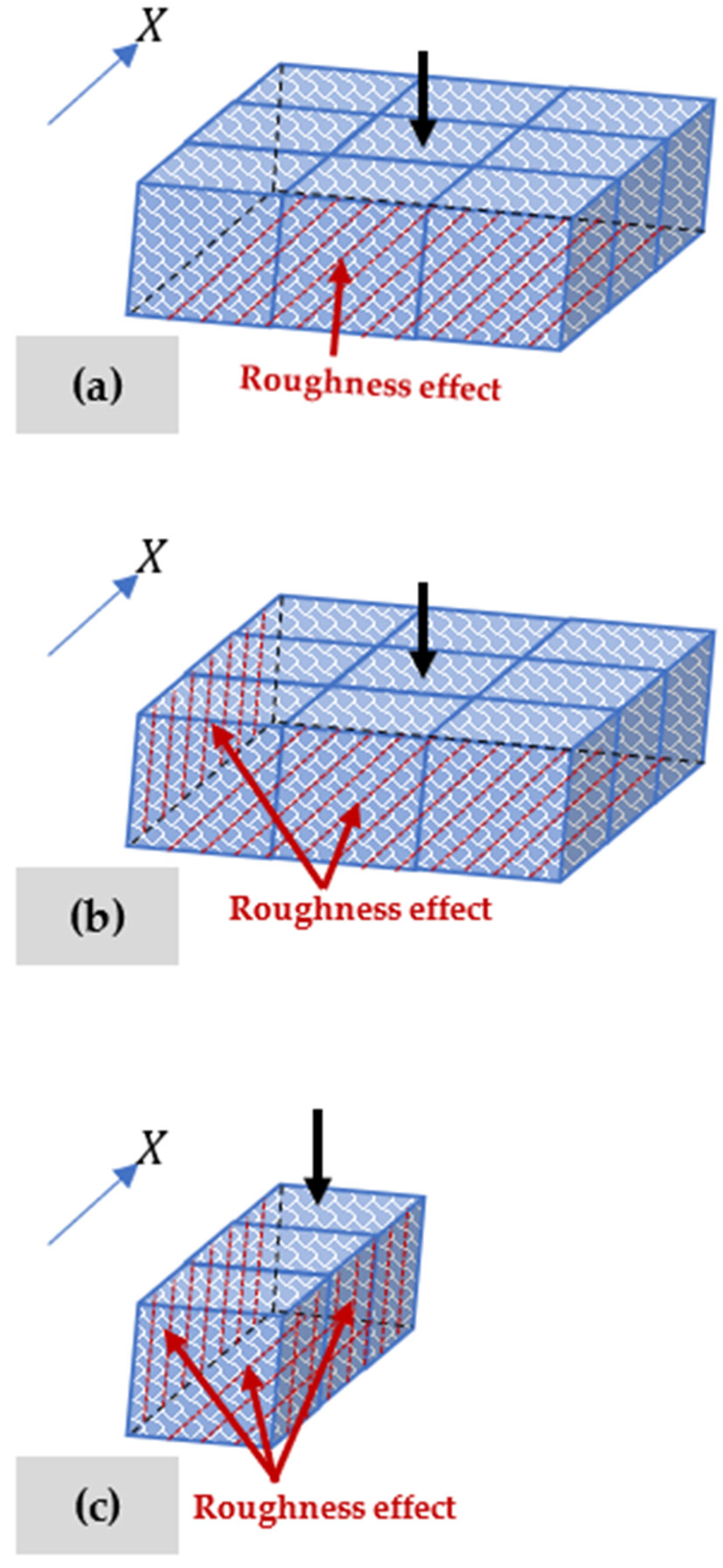
The hydraulic radius () will be given a specific treatment that more sensitively reflects the effect of bottom roughness and lateral walls. Therefore, the cases presented in Figure 3 are defined. Table 1 presents the definition of these cases.
Figure 3.
Defined cases for analysing hydraulic radius: (a) element within the domain; (b) element with one lateral wall; and (c) element with two lateral walls.
Table 1.
Definition of hydraulic radius in directions and .
The effect of the friction factor was included in Section 4.2 because theoretical solutions were available for comparison.
2.4. Boundary Conditions
In this section, four possibilities are analysed for having an open boundary to the sea with a given tidal condition, whether the boundary is to the left, right, top, or bottom of the shallow body being studied [25,32,33,34].
- (a)
- Flow in the direction, with an open-sea condition to the left, (Left):
For this condition, the following assumptions are considered:; and .
Equation (23) is transformed into the following expression:
- (b)
- Flow in the direction, with an open-sea condition to the right, (Right):
For this condition, the following assumptions are considered:; and . Then,
- (c)
- Flow in the direction, with an open-sea condition to the bottom, :
The assumptions considered are: ; ; and . Then,
- (d)
- Flow in the direction, with an open-sea condition to the top, (top):
For this condition, the assumptions are: and . Then,
- (e)
- Formulation of a channel in the direction
For a one-dimensional channel alienated in the direction:
The coefficient matrix for a one-dimensional channel has the form shown in Table 2. Here, the last term depends on the boundary condition
Table 2.
Coefficient matrix for a straight channel.
The open-boundary conditions are specified using a surface elevation function.
The simulation methodology considered the following forces: tides (water levels), winds (shear stress), surface-runoff inflows (rivers), and contributions and discharges through pipes or open channels. Only water levels were considered for validation testing, represented by a cosine or sine equation to simulate a long wave.
Engineers and designers can employ tidal components as desired, either as a single function or as individual superpositions of each tidal component.
Boundary conditions include an impermeable seabed, lateral walls, zero velocity, and water-level conditions at open boundaries.
2.5. Discretisation Scheme
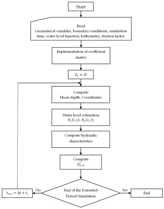
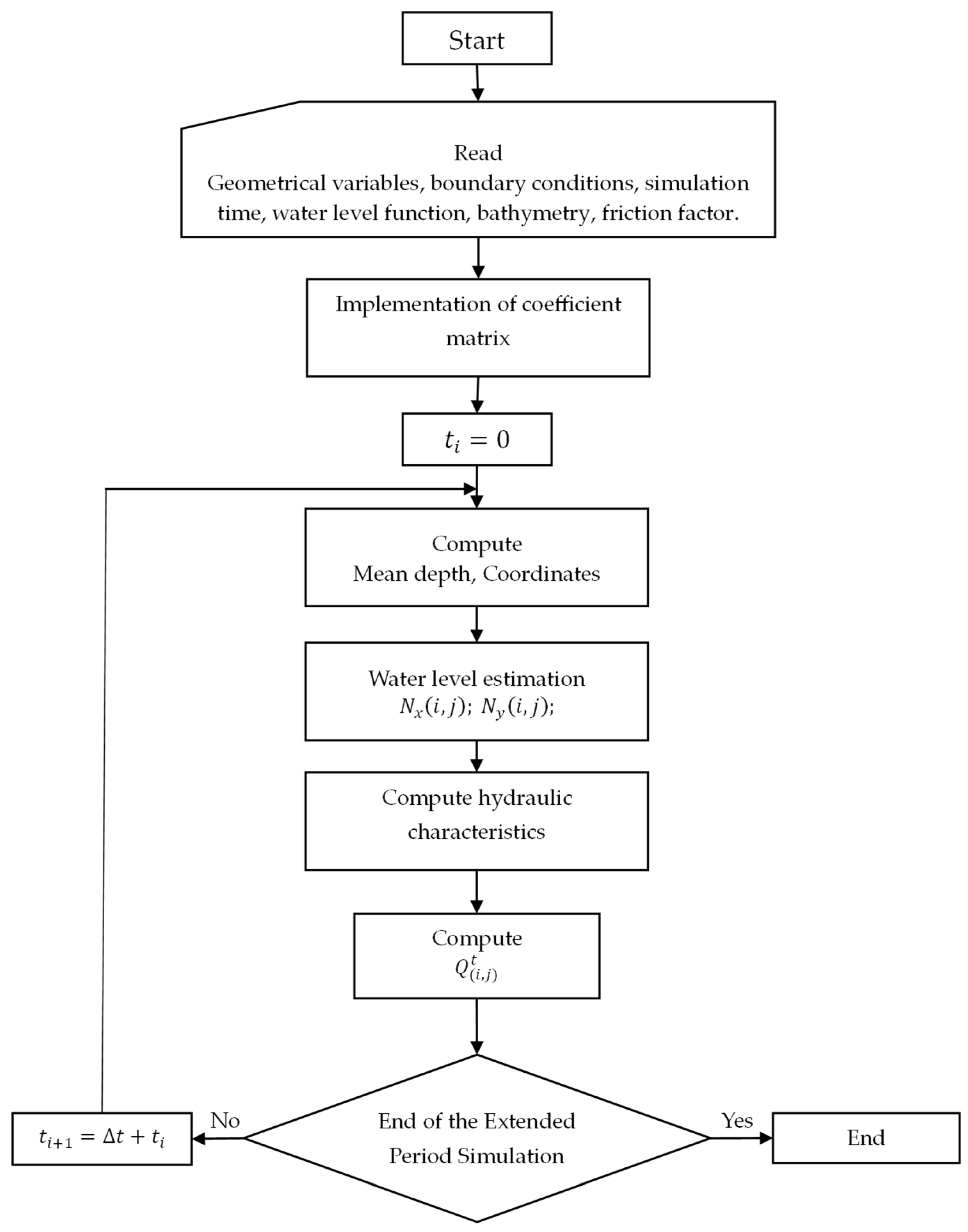
This section illustrates how the discretisation grids of the domain are considered (Figure A1). The blue line represents an open-boundary condition (left, right, top, and bottom) towards the sea. The water level is imposed in an analysed element. The flow rate is introduced as a new variable, which represents the flow in the X direction at the analysed element. Figure A2a presents the position of water levels along the contours of an element with (red) and (blue), along with the average water level at the centre of the element (green). Figure A2b shows the positions (red) where the depth or bathymetry values for the modelled area are introduced, as well as the representative position of the average depth computed with the proposed methodology (blue). Figure 4 presents the flowchart for applying the proposed methodology in this research.
Figure 4.
Flowchart for applying the simulation methodology.
Estimating levels in each of the elements into which the domain is discretised is one of the most significant aspects of ensuring the correct operation of this model. To calculate each of the coefficients of the solution matrix, it is necessary to know how the water surface level varies in space (X and Y directions).
This estimation is based on the theory of long-wave velocity in surface waters [25]. This velocity can be amplified or attenuated due to energy concentration effects, energy dissipation, bottom friction, and/or lateral wall friction. The procedure estimates the wave travel time from the boundary condition level (tide) to each element on its four sides. It is assumed that the level at each side of the element equals the boundary-condition level function at time , where represents the wave travel time influenced by a damping, dissipation, and/or amplification coefficient.
The level estimation functions may be analytical functions derived from linear theory and/or parametric functions obtained from field data.
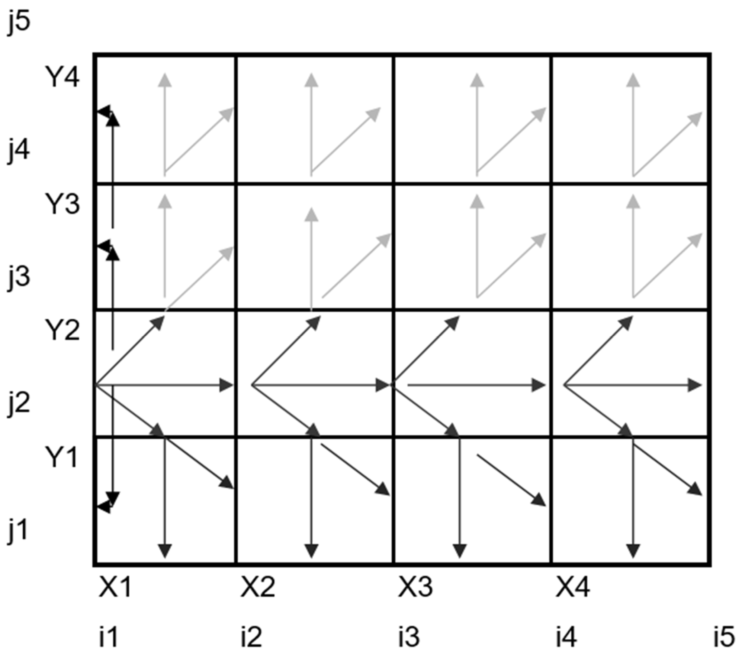
Figure A3 presents a representative scheme of the sequence in which levels are estimated for a boundary condition on the left side of the domain, considering the trajectories indicated by the arrows. Within the programming algorithm, the levels of the elements in the cell containing the boundary-condition level are initially estimated. This is followed by the estimation of levels in the cells above, then in the cells below, and finally, in the first row (), both above and below the boundary-condition level.
3. Results
To validate the modelling methodology proposed in this research, the simplified hydrodynamic model (proposed model) was compared to the analytically obtained results for a one-dimensional rectangular channel with one open end (known water-level condition) and one fully reflective closed end (zero-flow condition).
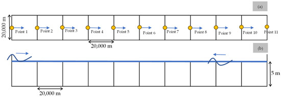
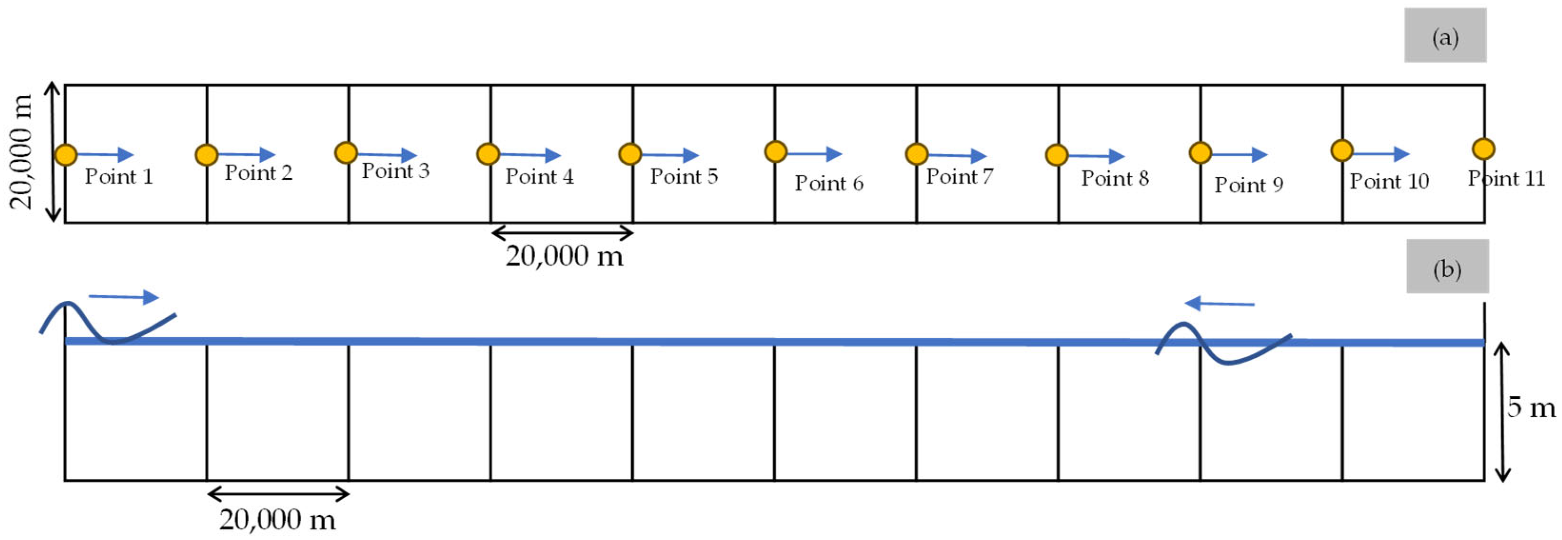
For the analysis, a channel with a length of (where is the wavelength) and a width of has been considered, divided into 10 elements of a similar length, with a constant depth h (5 m).
A rectangular channel measuring 20,000 m in width and 200,000 m in length was analysed to assess the model’s sensitivity. The length was divided into 10 elements, each 20,000 m long. As a result, each element is square-shaped, with dimensions of 20,000 m in width and 20,000 m in length (Figure 5). Points 1–11 are identified to observe the behaviour of some variables.
Figure 5.
A schematic of the rectangular channel discretization into ten elements: (a) plan view; and (b) profile view.
3.1. Neglecting the Friction
For this scenario, a cosinusoidal wave with a height (0.5 m) and a period (24 h) is used as the incident wave.
This wave is propagated through the channel and combined with the reflected wave.
Table 3 presents the matrix coefficients for the one-dimensional rectangular channel, where the terms correspond to the time-independent terms at time
Table 3.
Coefficient matrix for the case study.
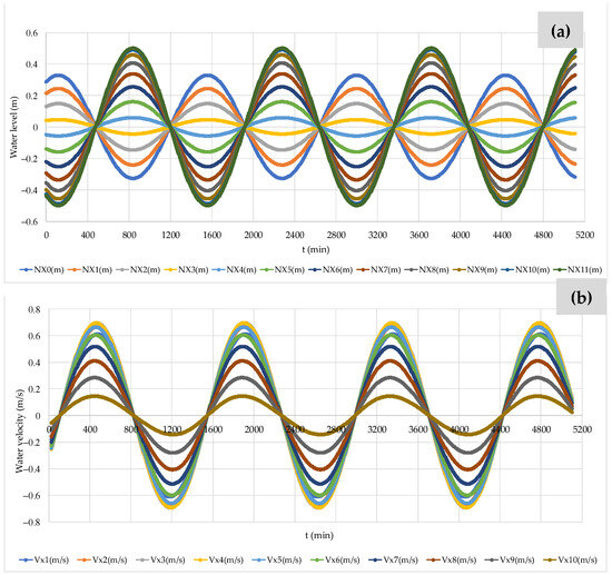
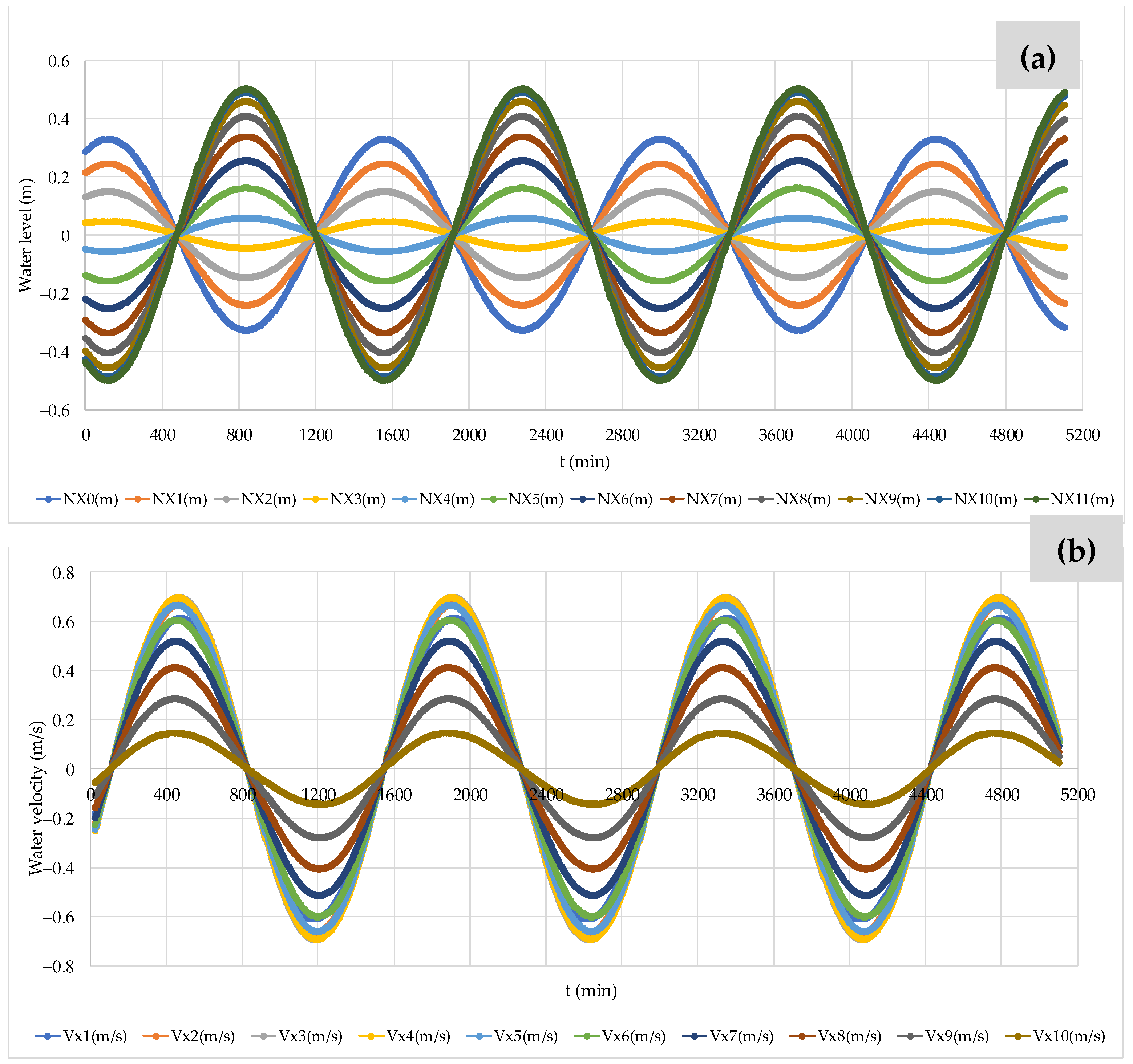
Figure 6a compares the estimated water levels at each position in the channel, corresponding to the elements into which the channel has been divided. It shows that the first three water levels are out of phase with the last seven. The velocities calculated by the model for each discretisation element are shown in Figure 6b, where it can be observed that they are all in phase. The maximum water level computed by the proposed model at Point 11 is 0.499 m (i.e., at 3720 min), whereas the maximum velocity has a value of 0.159 m/s for Position 5.
Figure 6.
Analysis of variables computed by the proposed model neglecting the friction: (a) water levels; (b) water velocity.
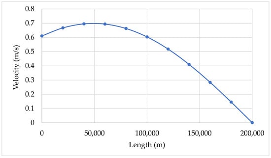
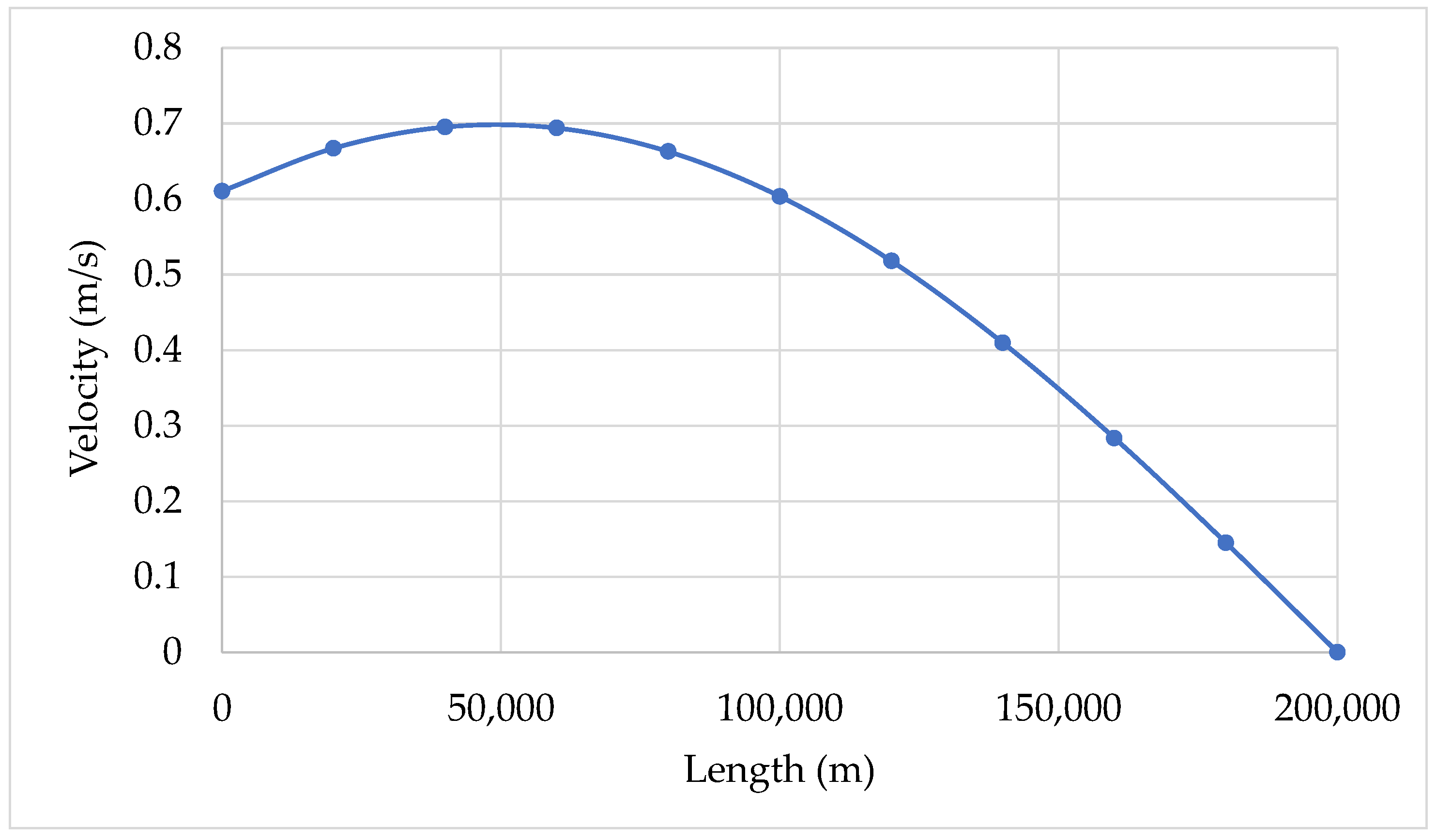
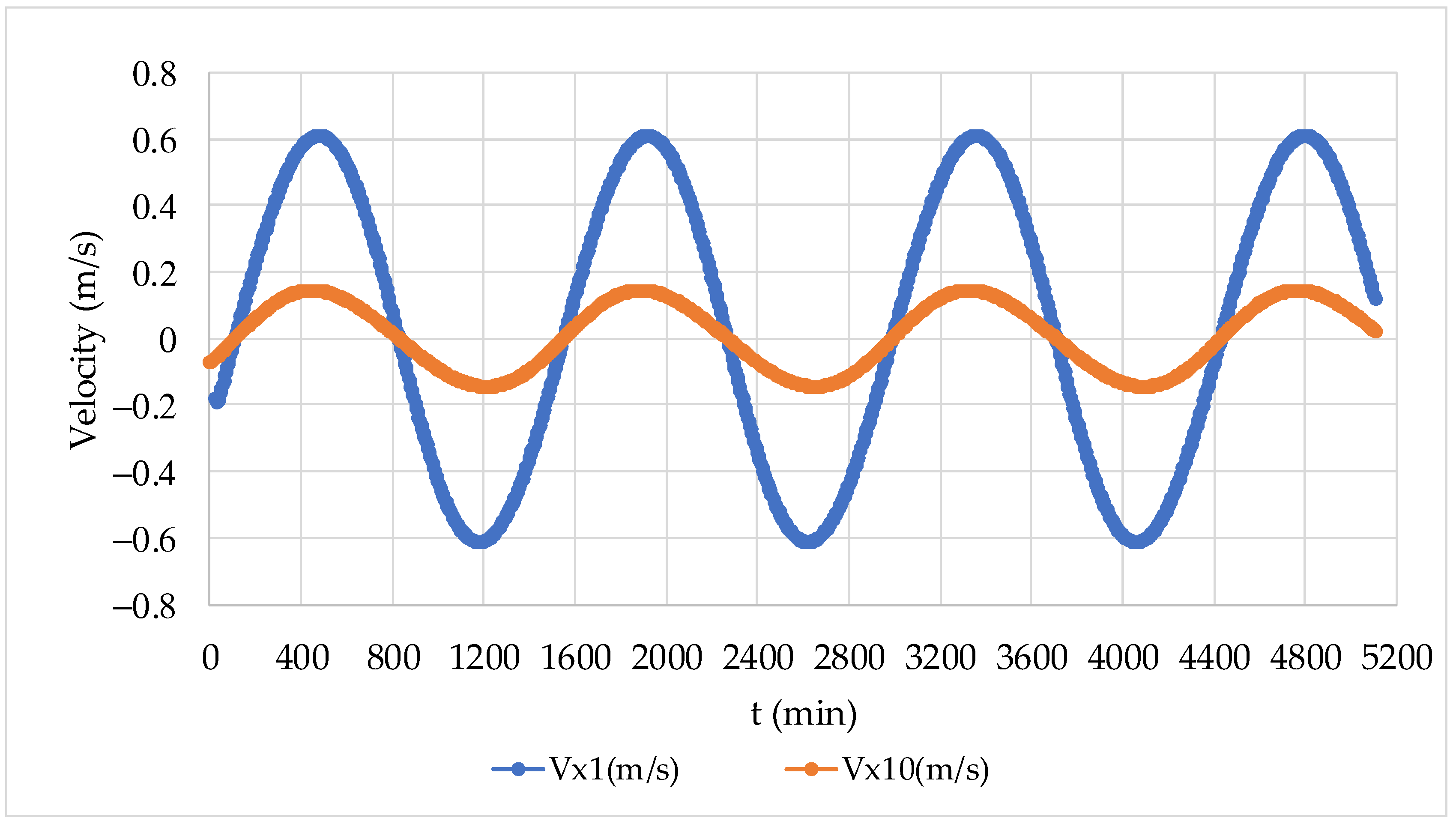
Figure 7 shows a longitudinal profile of the velocity along the channel as a function of the wavelength, aimed at validating the longitudinal behaviour of the velocity and the presence of the velocity node at , which the model accurately reproduces. Along the channel, the maximum velocity is 0.695 m/s, which occurs at a distance of 40,000 m. Figure 8 shows the behaviour of velocity and level at positions one and ten in the model’s discretisation. The proposed model is suitable for wave routing, where the maximum values of velocities for positions 1 and 10 are 0.611 and 0.145 m/s, respectively.
Figure 7.
Longitudinal profile of maximum velocity.
Figure 8.
Velocities are calculated at positions one and ten.
3.2. Considering the Bed Friction
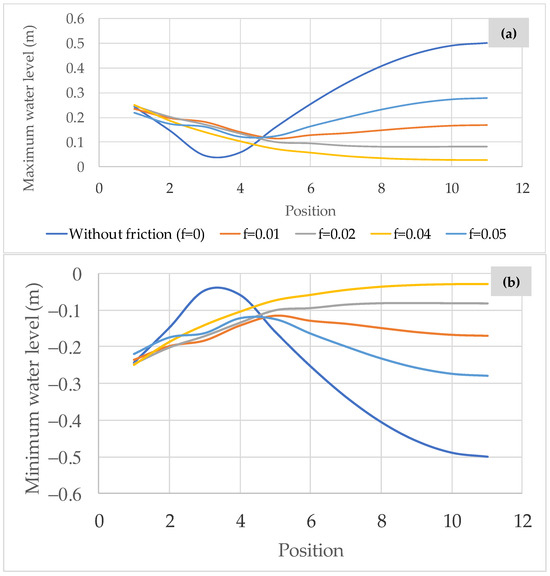
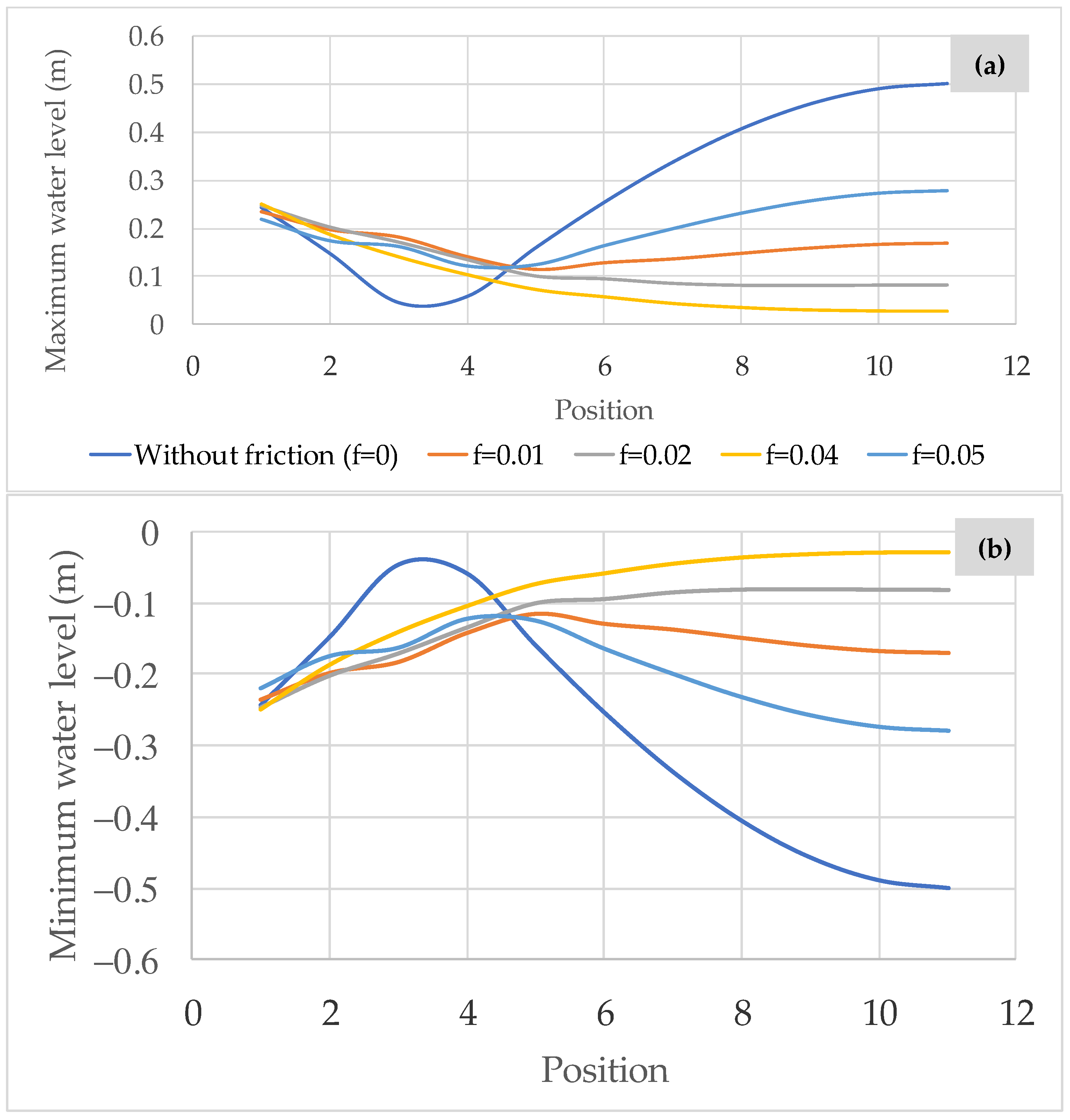
This section includes the effect of level damping due to bottom friction in the wave propagation. The proposed model was applied for friction factors () of 0.005, 0.01, 0.02, and 0.04, as illustrated in Figure 9. The results were compared to the scenario where the friction factor is disregarded. It was observed that the higher the friction factor, the lower the maximum water levels attained (Figure 9a). For instance, considering a friction factor of 0.005, a value of 0.27 m is observed at Position 11, whereas for a friction factor of 0.04, a maximum water level of 0.03 m is achieved. Figure 9b shows the minimum attained water levels.
Figure 9.
Analysis of water levels considering different values of friction factor: (a) maximum water levels and (b) minimum water levels.
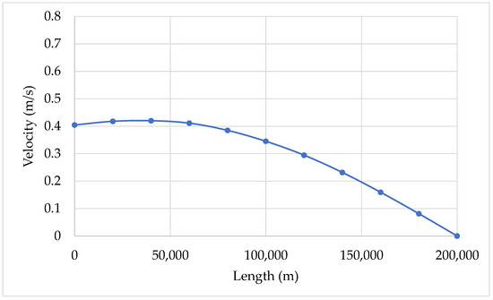
In addition, Figure 10 presents a longitudinal profile of the velocity to illustrate the effect of the friction factor for a value of 0.05. The behaviour is similar to that without friction but with a maximum magnitude of 40% lower. In this case, the maximum velocity is 0.424 m/s, which occurs at a distance of 69560 in the rectangular channel.
Figure 10.
Longitudinal profile of reached maximum velocities for .
4. Discussion
4.1. Neglecting the Bed Friction
The simplified hydrodynamics model was compared to the analytical solution for the water level and velocity at each position along the channel, according to linear theory for a rectangular channel without friction. In this sense, the following equations were employed:
where = channel length, = incident wave level, and = the sum of the incident wave level and reflected wave.
The horizontal velocity () in the direction is yielding by
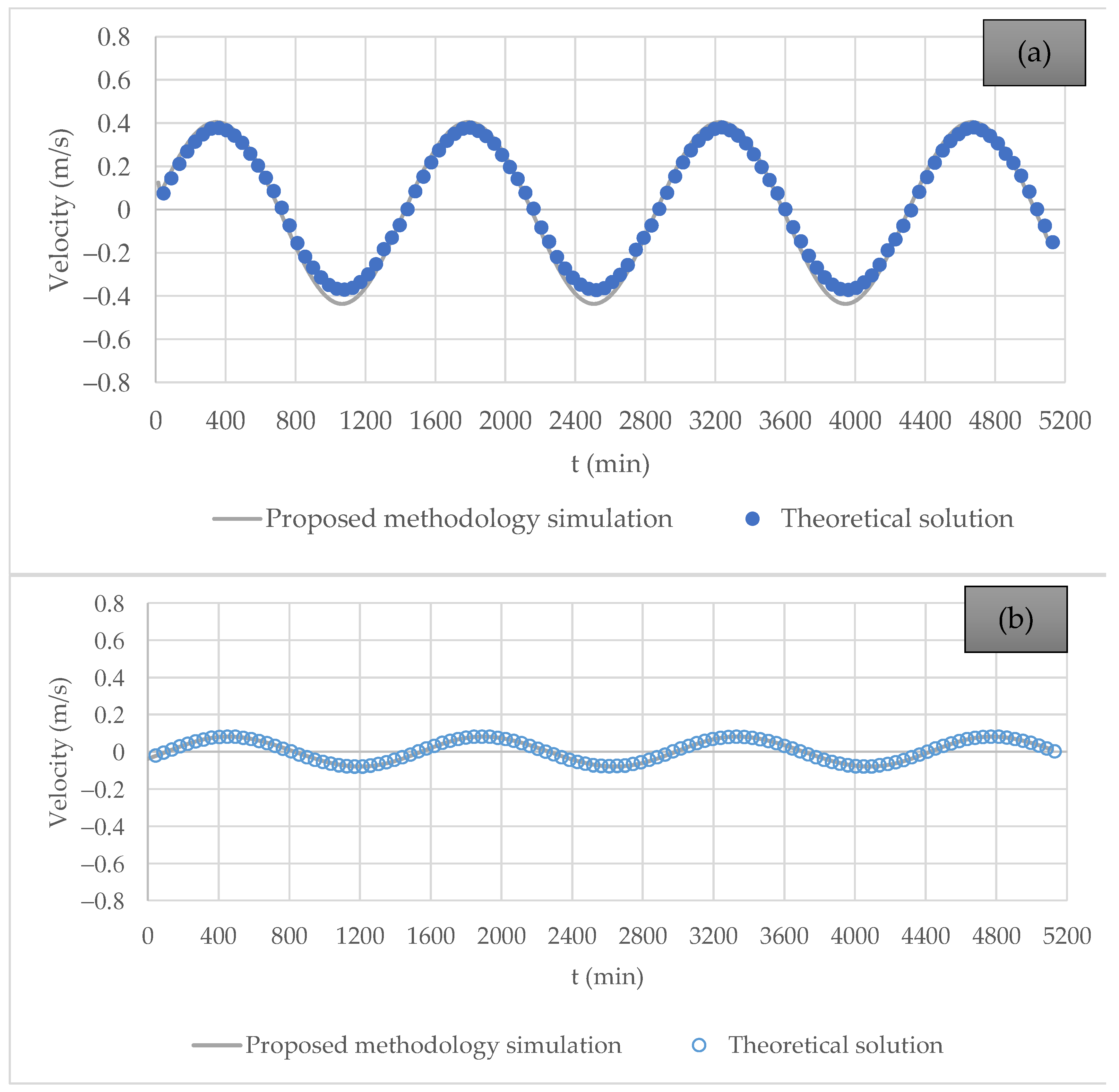
Figure 11 shows the results obtained by the proposed methodology for two positions within the rectangular channel: one at the open-boundary condition (1) and a second at the element with a zero-flow boundary condition on the right (10). The results shown in the graphs are relatively similar.
Figure 11.
Comparison of water velocity between the proposed model and linear theory neglecting the bed friction: (a) Position 1 (inlet channel); and (b) Position 10 (last element).
To evaluate the proposed simulation methodology about linear theory, the correlation coefficient () was computed as follows:
where represents the velocity calculated using the proposed simulation methodology, is the velocity obtained from linear theory, and is the number of analysed points.
The was computed for the velocity oscillations presented in Figure 11, yielding values of 0.9998 and 0.9988 for Positions 1 and 10, respectively. These results demonstrate that the proposed methodology provides values that closely agree with the linear theory.
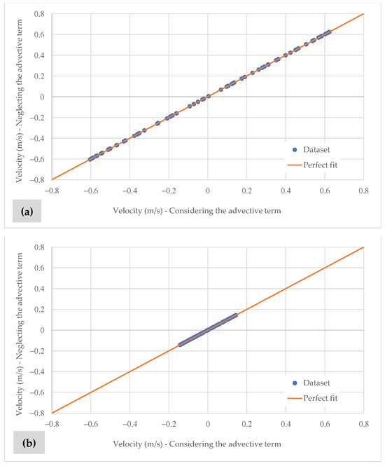
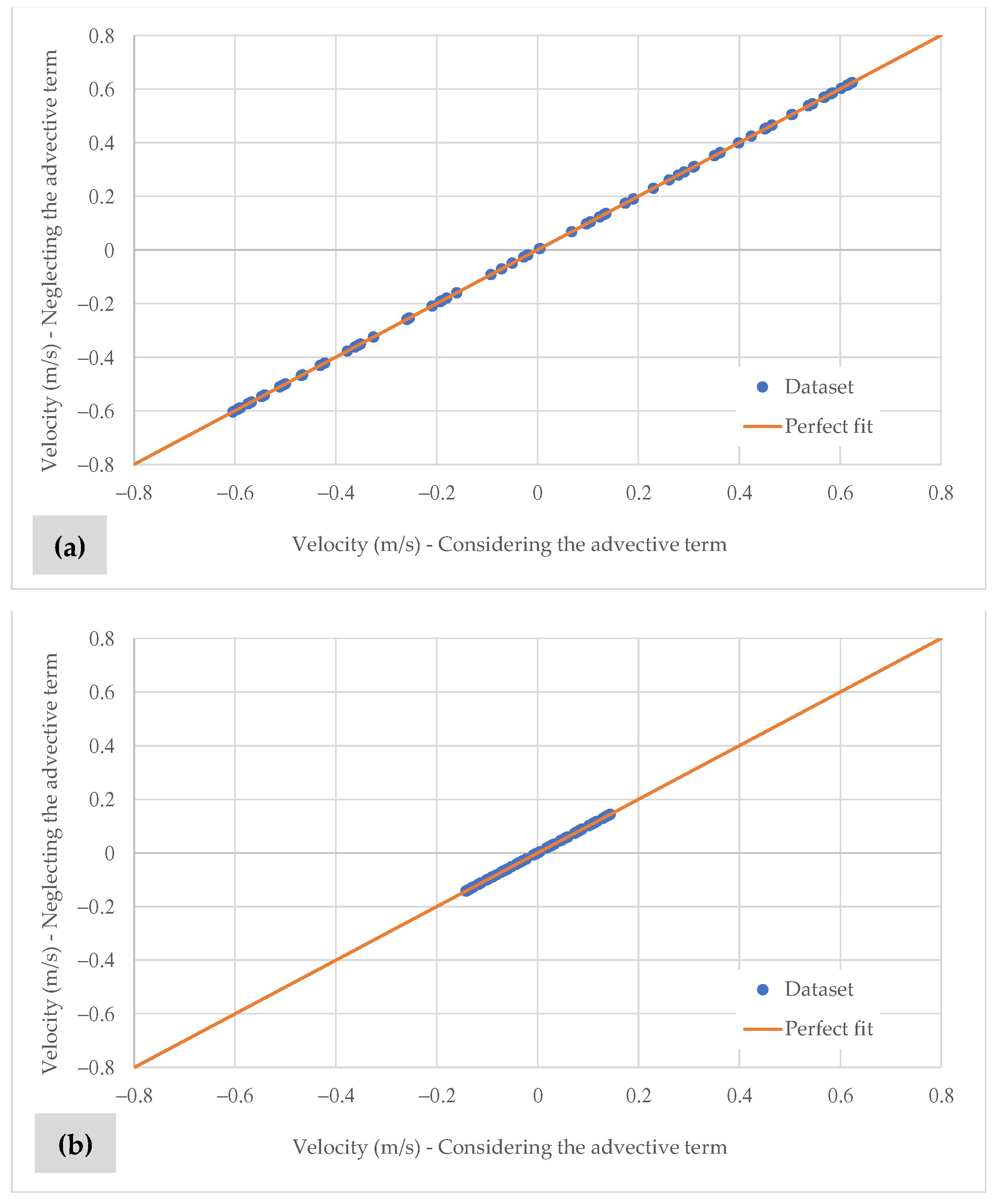
A second analysis was conducted to evaluate the effect of including or excluding the advective terms in the model. Figure 12 shows that this effect is negligible, as expected, given that the channel is one-dimensional. Again, the proposed simulation methodology proves suitable for modelling this scenario.
Figure 12.
Effect of the advective terms: (a) Position 1 (inlet channel); (b) Position 10 (last element).
4.2. Considering the Friction
The damping effect is described by the linearised solution presented in Reference [25], which expresses the relationship between the wave level at two points in the channel. This expression is determined as follows:
where = friction factor coefficient, = modulus of maximum velocity, = depth, , , = original wavelength, = period, = level at zero distance, and = level at distance.
For a horizontal velocity of a progressive wave [25], the following expression has been found:
By subtracting the velocity of the reflected wave from the velocity of the incident wave, the following theoretical equation is obtained for calculating the horizontal velocity in a channel of length :
The terms and are computed as:
The friction coefficient classification was established according to the following criterion [35]: (a) for a low friction coefficient, ; and (b) for a high friction coefficient, . The value can be computed as , where . is defined as maximum velocity modulus.
Data presented as follows have been considered: , m/s, s, m, and . According to Prandle’s classification [35], the friction used falls within an intermediate range.
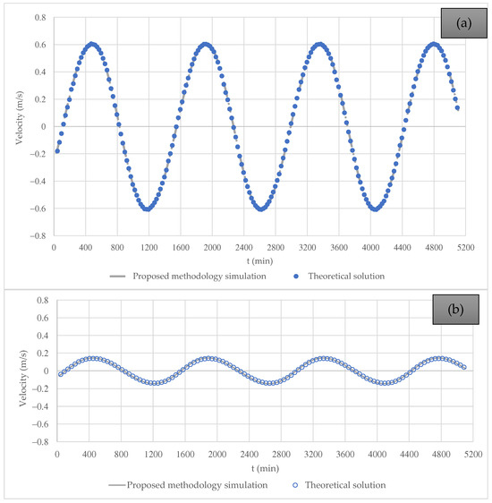
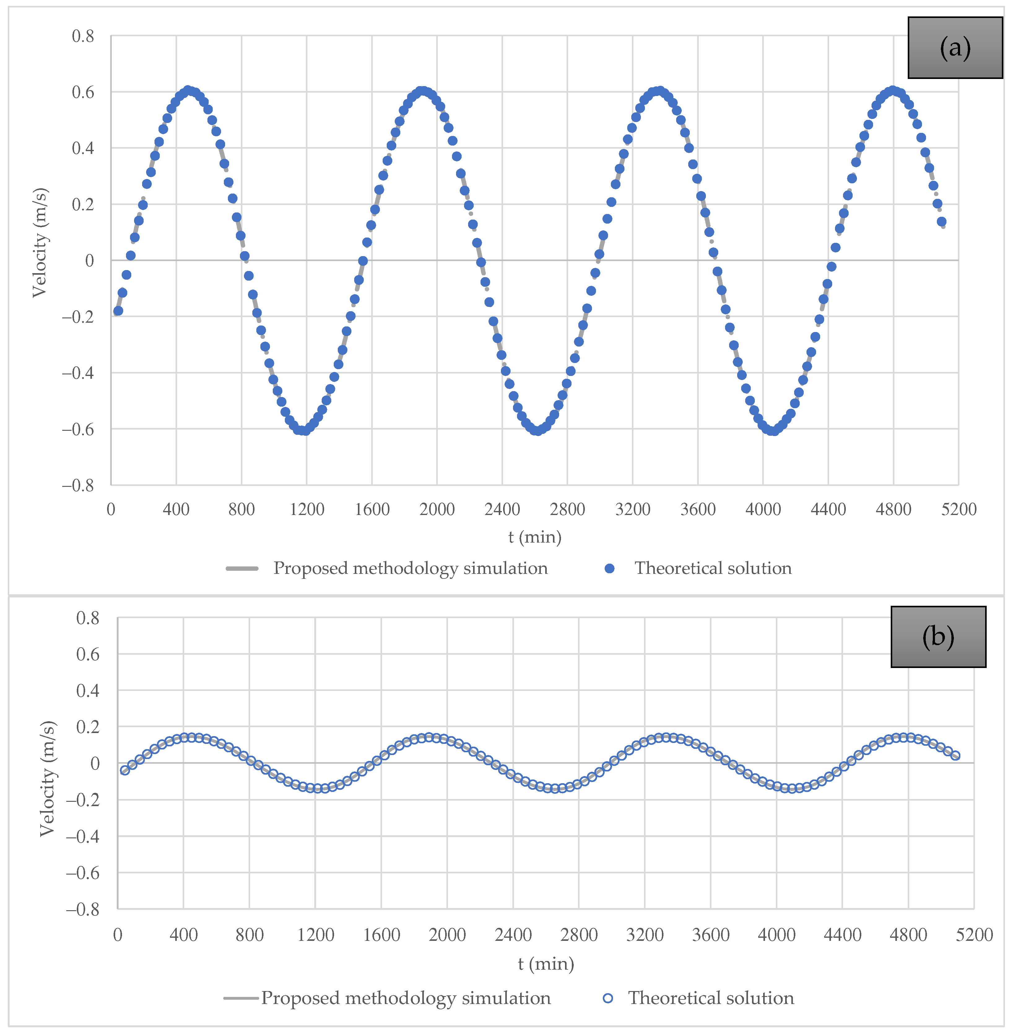
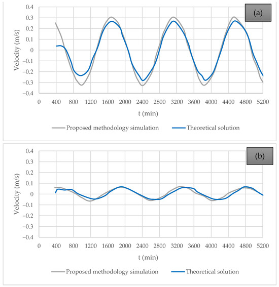
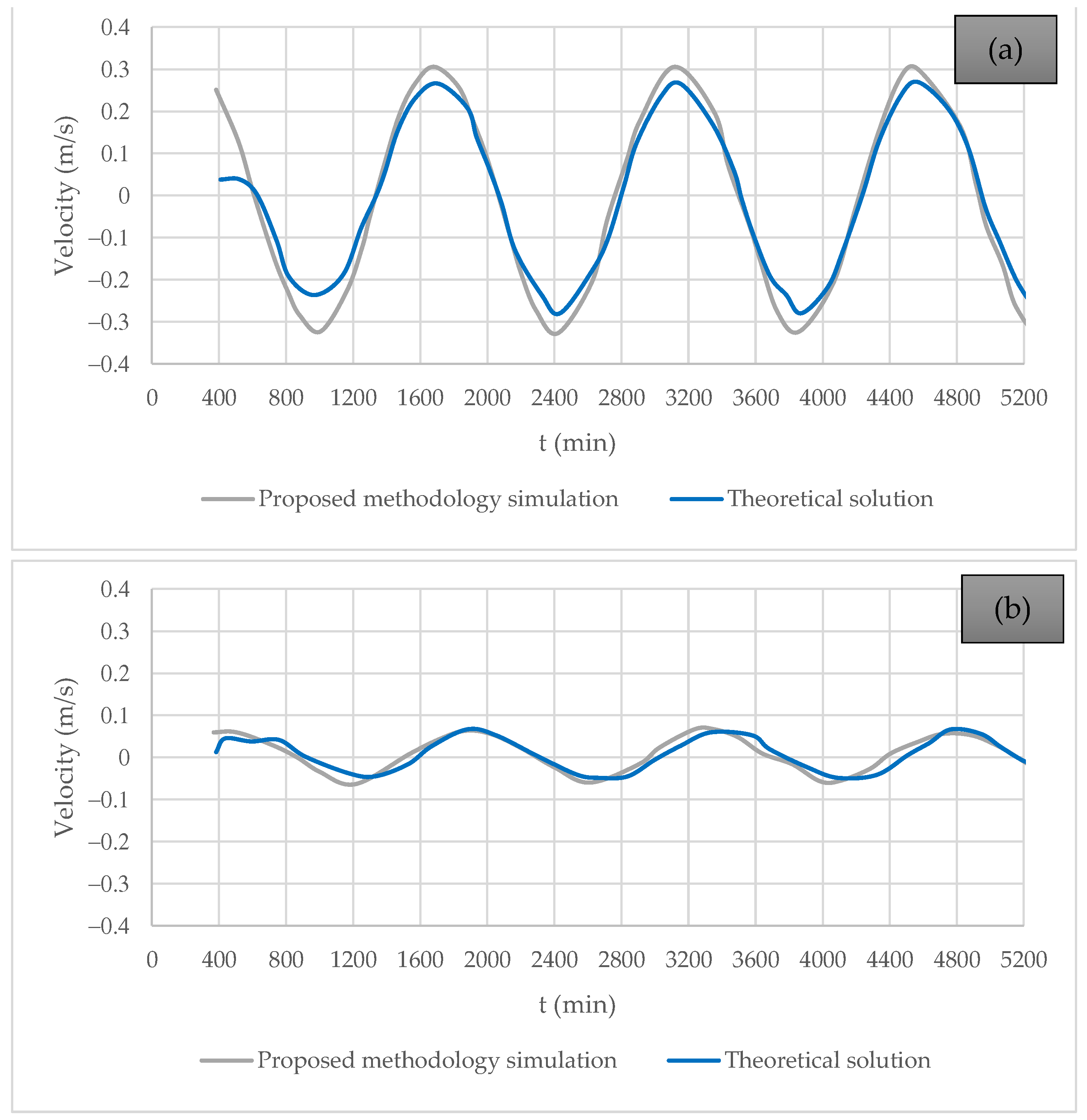
Figure 13 compares the theoretical equations and the proposed methodology (simplified hydrodynamic simulation methodology) for Positions 1 and 10. Both models present similar results.
Figure 13.
Comparison of water velocity computed using the proposed methodology and the theoretical formulation using = 0.005: (a) Position 1 (inlet channel); and (b) Position 10 (last element).
For Positions 1 and 10, the values are 0.9975 and 0.9947, respectively, again demonstrating the suitability of the proposed approach.
The proposed simulation methodology is an alternative for modelling hydrodynamics in bays and estuaries. It is a valuable tool, particularly in regions with limited data availability, as it is well-suited to reproducing the wave phase in scenarios with impermeable walls.
The proposed simplified simulation methodology is potentially more applicable to engineering solutions that rely on average or extreme values, serving as a support tool for decision making. In this case, wind acts as a surface shear stress and is included in the formulation. However, it was excluded from the initial model test to minimise noise during the validation process.
It is of utmost importance to mention that linear theory can be applied when the principles of additivity and multiplicativity are present. At the same time, the proposed simulation methodology corresponds to an approximation that can be employed when these principles are not fulfilled.
4.3. Analysis Using an Exponentially Varying Width
The width was exponentially varied to compute the behaviour of the hydrodynamic model for the analysed interconnection. The simulation was performed using the conventional model and the hydrodynamic model presented in this research, using a friction coefficient (f) of 0.01 and an exponential variation coefficient in the width with . A constant depth of 5 m was used for the analysis.
For modelling considering the theoretical solution, the following equations were used:
where = water level to a distance at time , = velocity to a distance at time , = initial width () in the channel at the wall (15,000 m), = channel width, and = amplitude in the wall ().
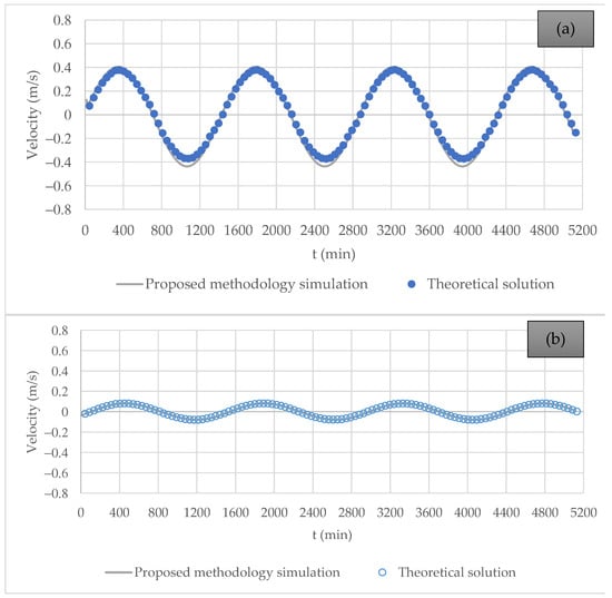
Figure 14 shows the velocity component results for elements 1 and 10, illustrating that the proposed methodology simulation is suitable for representing velocity compared to the theoretical solution. It is essential to highlight that the hydrodynamic model appropriately describes the wave phase.
Figure 14.
Comparison of water velocity for an exponentially widening channel, computed using the proposed methodology and the theoretical formulation with = 0.01: (a) Position 1 (inlet channel); and (b) Position 10 (last element).
4.4. Application of the Proposed Methodology Simulation to a Case Study
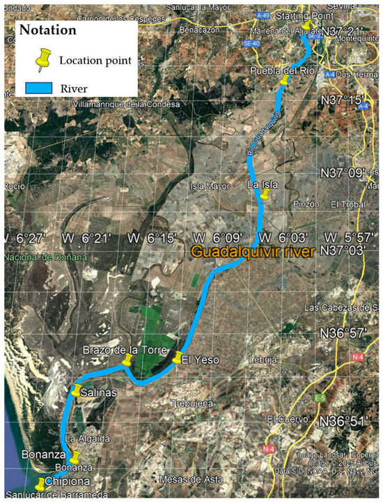
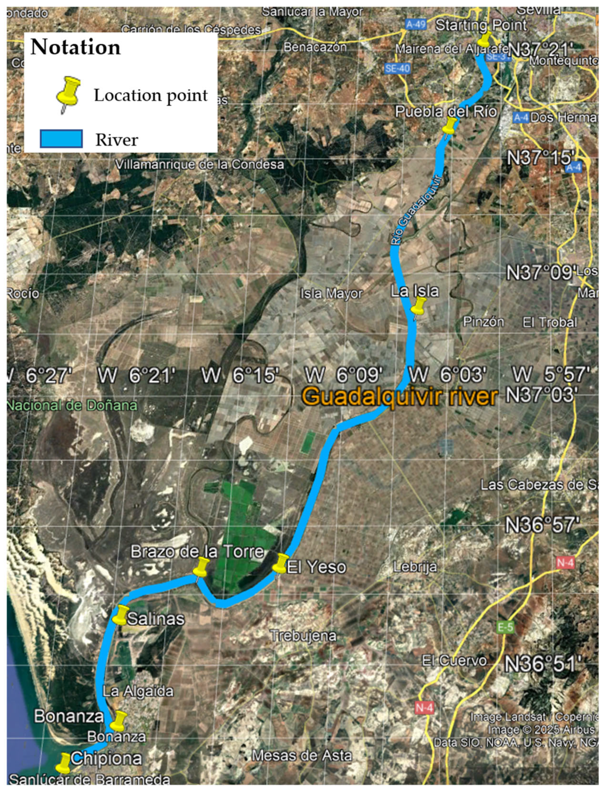
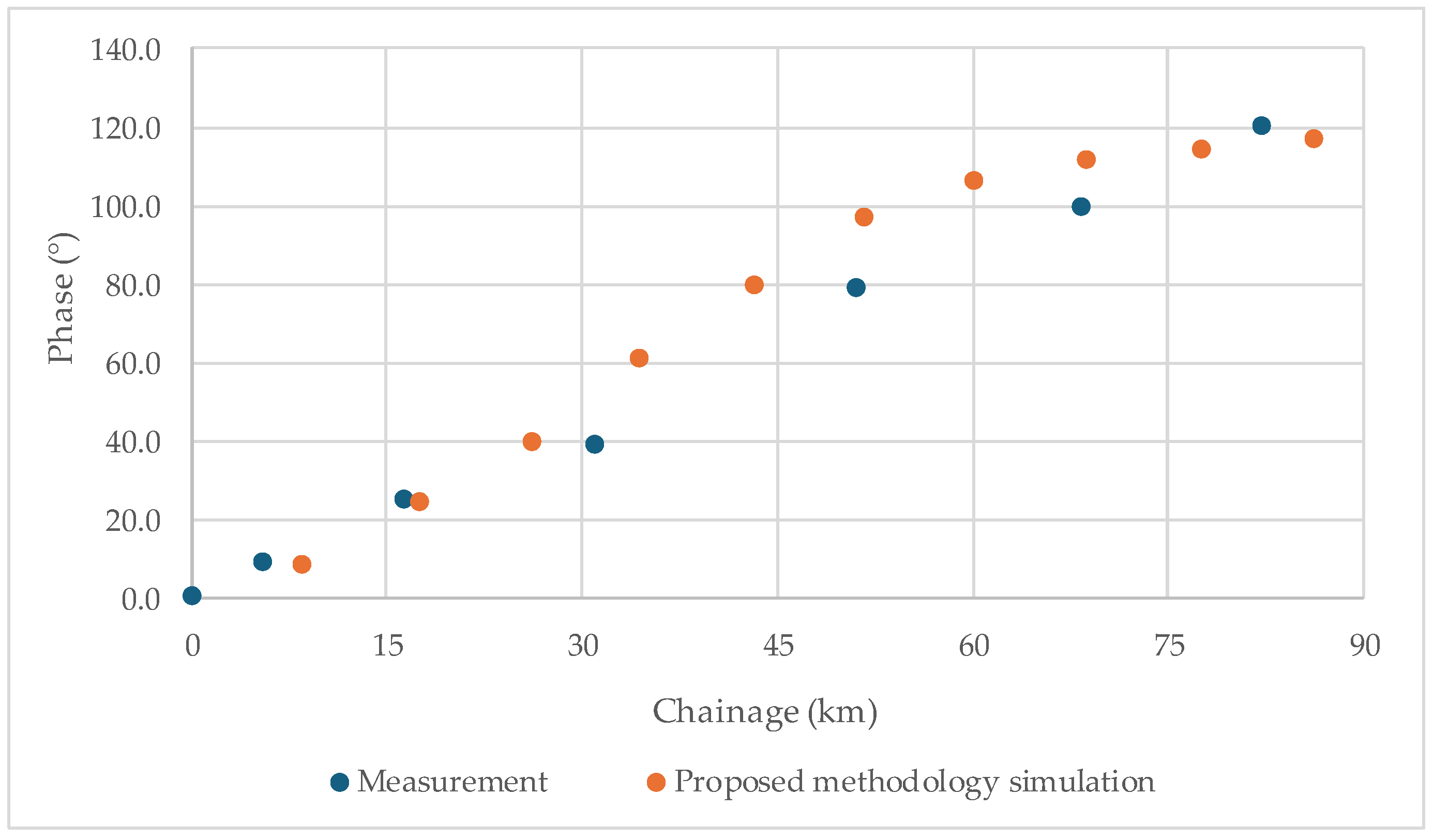
This section examines the amplification phenomenon of the M2 tidal component in the Guadalquivir River, as recorded by the University of Cádiz, Spain [31]. The corresponding amplitudes and phases along the channel are presented in Table 4. Figure 15 presents the location of the measurements along the Guadalquivir River.
Table 4.
The amplitude of the M2 tidal component along the Guadalquivir River (Spain).
Figure 15.
Location of the case study.
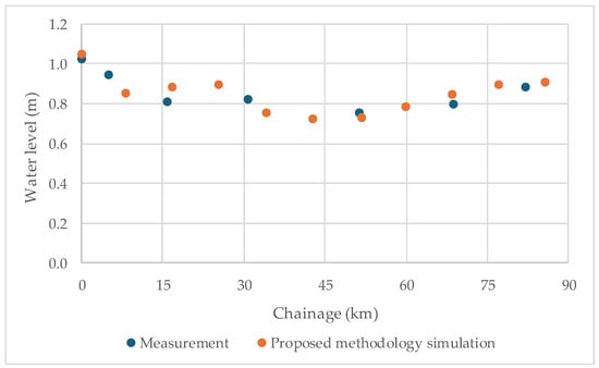
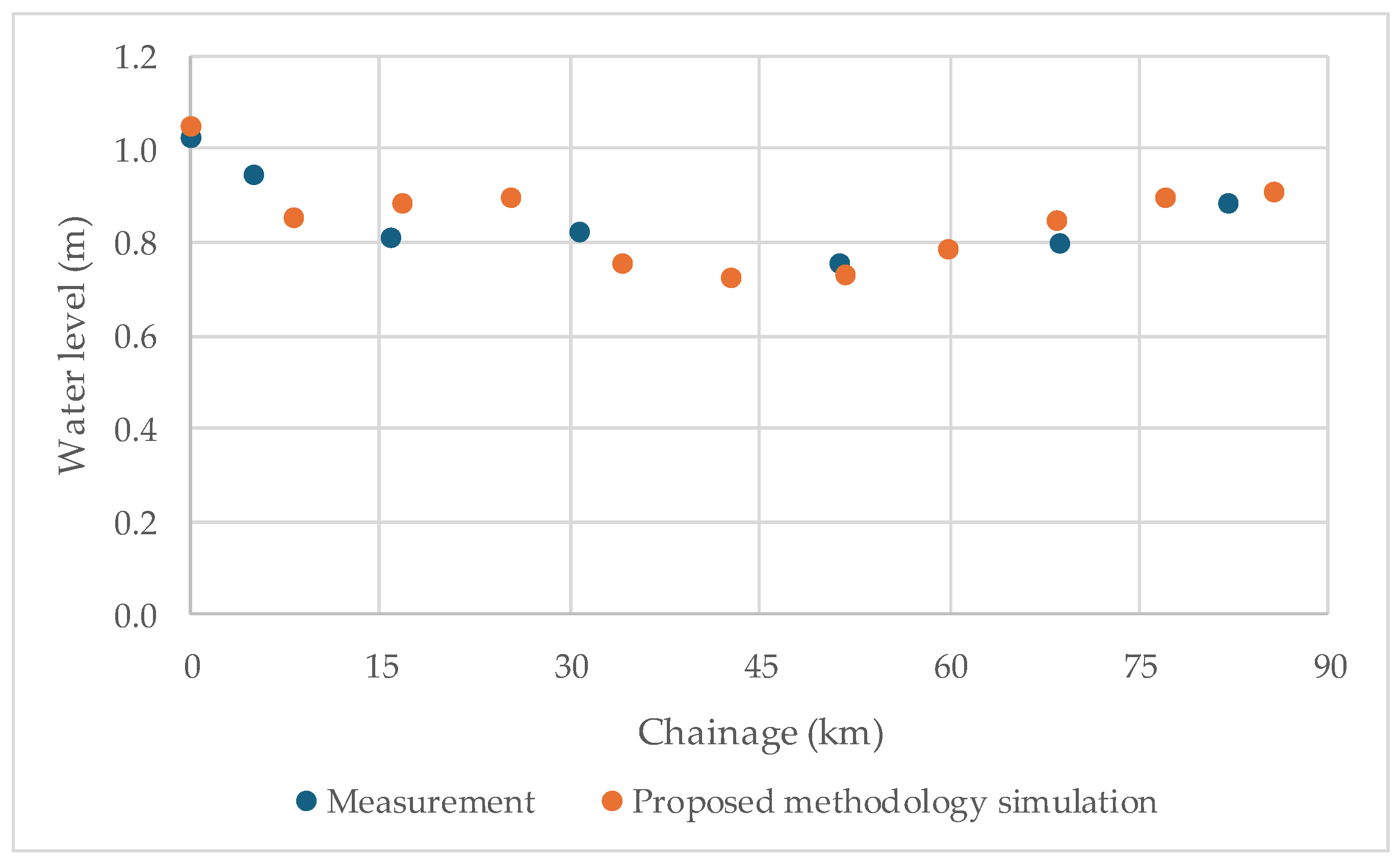
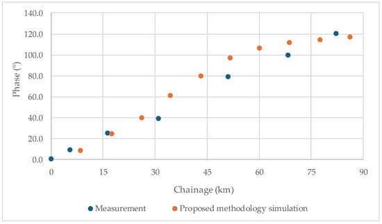
The model was used as input data for a period of T = 735 s, with an incident wave height of 2.2 m and a bed-friction coefficient () of 0.012. Figure 16 presents the wave amplitude profile along the channel, comparing field measurements (blue) with modelled results (orange), which have been adjusted using the bed-friction coefficient. Similarly, Figure 17 displays the phase results, showing the phase difference relative to the channel entrance (Chipiona).
Figure 16.
Longitudinal profile of the amplitude along the channel.
Figure 17.
Longitudinal profile of phase relative to the channel entrance (Chipiona).
5. Conclusions
This research presents the development of a hydrodynamic simulation methodology for estuaries and bays that prioritises practical applications. The methodology was developed based on a vertically integrated model. The proposed method is straightforward, producing a unique solution that converges quickly and independent of initial flow values. The simplicity of the simulation methodology is further underscored by the fact that it requires only one calibration parameter: the bed-friction coefficient. Compared to current hydrodynamic models, the main advantage of the proposed simulation methodology is its significantly reduced need for parameter calibration.
It is demonstrated that more complex models necessitate a significantly more significant number of parameters. While the methodology remains straightforward and appealing for engineering applications, it is essential to note that as the number of parameters increases, so does the computational cost. Furthermore, including additional parameters does not invariably lead to more accurate solutions, highlighting a potential trade-off between complexity and precision.
Consequently, it also reduces computational time. Compared with linear theory, the proposed methodology demonstrated its suitability for representing the wave phase, making it a practical tool for computing water levels and velocities in bays and estuaries.
The proposed methodology’s flexibility is evident in its ability to accommodate varying discretisation in both the X and Y directions. Additionally, in narrow and deep channels, the methodology’s proposed hydraulic radius within the bed-friction equation better captures the influence of channel sidewalls on flow magnitude. The proposed methodology’s sensitivity to the bed-friction coefficient is particularly advantageous from an engineering standpoint, as it facilitates the examination of hydraulic structures with varying roughness and their impacts on circulation. Furthermore, velocity results in the X direction remain consistent regardless of the number of elements used. Overall, the proposed simulation methodology is versatile and easy to implement using any system of equations, with the accuracy of the simulation methodology being closely tied to the quality of initial level estimation, whether determined analytically, empirically, or through a combination of both methods.
Future research should focus on applying the simulation methodology to real-world case studies, mainly where bidimensional flow effects are present. The simulation methodology ought to be compared with existing hydrodynamic models. Furthermore, the methodology’s implementation within a commercial software package could be developed to analyse hydrodynamics in practical scenarios. The proposed simulation methodology is formulated in Cartesian coordinates, requiring a higher discretisation level for complex coastlines.
Author Contributions
Conceptualization, A.A.-P.; methodology, A.A.-P. and O.E.C.-H.; formal analysis, A.A.-P.; validation, A.A.-P.; writing—original draft preparation, A.A.-P.; writing—review and editing, V.S.F.-M. and O.E.C.-H. All authors have read and agreed to the published version of the manuscript.
Funding
This research received no external funding.
Data Availability Statement
Databases are available in this article.
Conflicts of Interest
The authors declare no conflicts of interest.
Appendix A. Derivation of Equations
This appendix aims to quantify the order of magnitude of each component of the equation to identify which terms can be neglected and which must be retained, as well as the conditions under which these approximations are valid
By differentiating Equation (4) with respect to time and space:
and,
Establishing the relationship ; then, , which represents the spatial and temporal variations in velocity as they relate to wave characteristics. The average ratio is yielded by:
where .
From the above, it is concluded that, on average, the relationship between the first-order term and the advective term is , given the ratio of . Generally, the minimum average value of the absolute relation between the first-order term and the advective term is greater than .
Applying a similar procedure to the momentum equation in the direction and using the expression for the vertical velocity (Equation (5)), differentiating concerning both time and space, yields:
Considering the advective term to the first-order term:
The average value of this relationship is yielded by:
The relationship between the first-order term and the advective term is:
The relationship between the first-order and advective terms is the same for both the horizontal and vertical directions according to the momentum equation. The third term in the momentum in direction is:
Establishing the relationship between the first-order term and the advective term results in:
The average value of the relationship between the first-order term and the advective term is yielded by the integral of Equation (A9) between and .
Appendix B
The advective terms in Equation (6a) are the smallest and can be neglected; as a consequence, the momentum equation in the direction can be simplified as:
The integration of the mass conservation equation along the depth [5], expressed in terms of the mean velocities, is described as follows:
Based on the momentum equation and integrating along the axis, then:
Deriving about the :
The vertical velocity for a long wave is yielded by:
By deriving Equation (A18):
The second term on the right side of Equation (A13) can be expressed as:
Integrating along , then:
Organazing terms:
Then,
Expanding some terms, then:
Then,
By plugging Equation (A25) into Equation (A13), then:
Applying Equation (A19) for and then:
where
Deriving concerning and , then:
Neglecting the second-order terms in Equations (A28) and (A29) since is independent of and , substituting into the momentum Equation (6b,c), and expressing the partial derivative of the velocity in as a function of the derivative of the velocity with respect to , the following expressions are obtained:
Since is close to 1, has an order of magnitude of 10−9, and the horizontal velocity for long waves is uniform with respect to the depth, the mass conservation and momentum equations can be expressed in terms of the mean horizontal velocities ( and ) and the surface velocity as follows:
Appendix C
Figure A1.
Scheme of the discretisation domain: (a) intermediate position; (b) boundary condition at left level; (c) boundary condition at right level; (d) boundary condition at top level; and (e) boundary condition at bottom level.
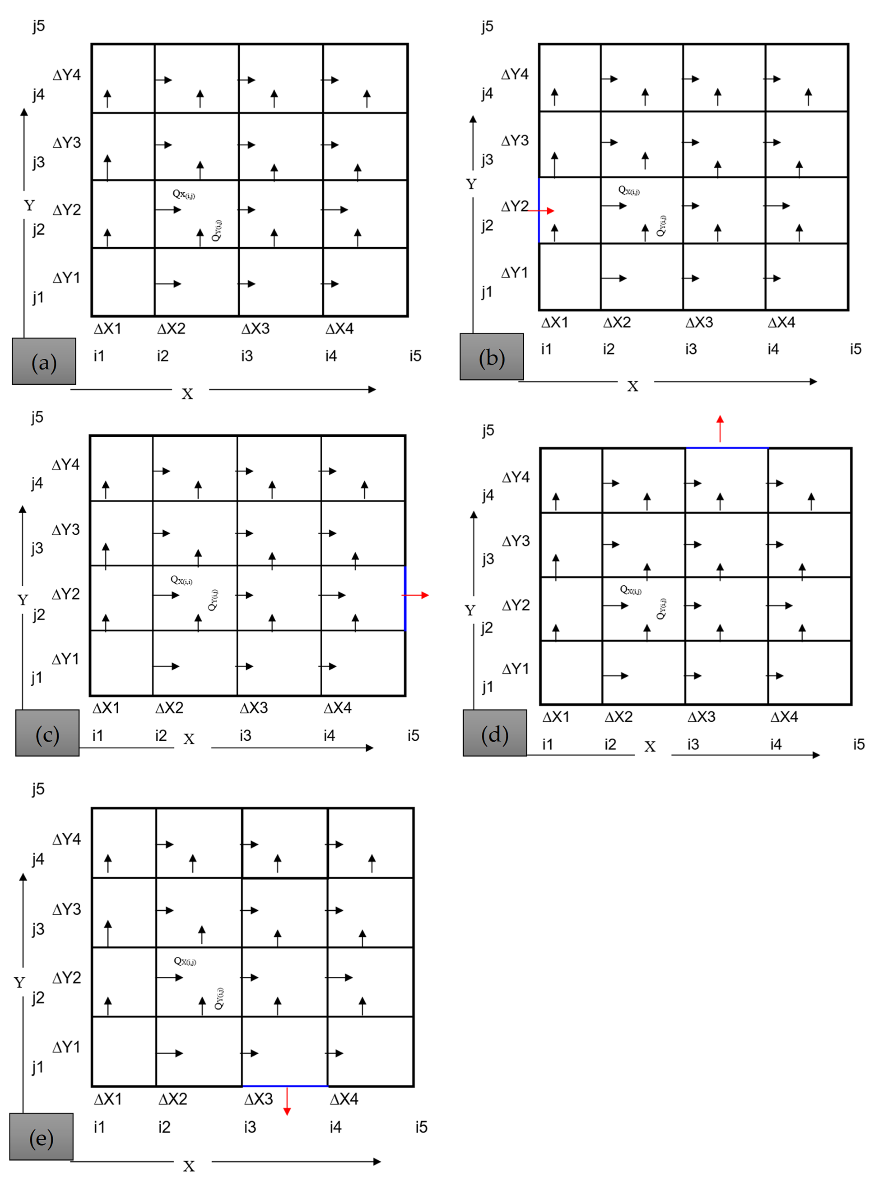
Figure A2.
Scheme of location points: (a) position of level of each element; and (b) position of bathymetric points for modelling purposes.
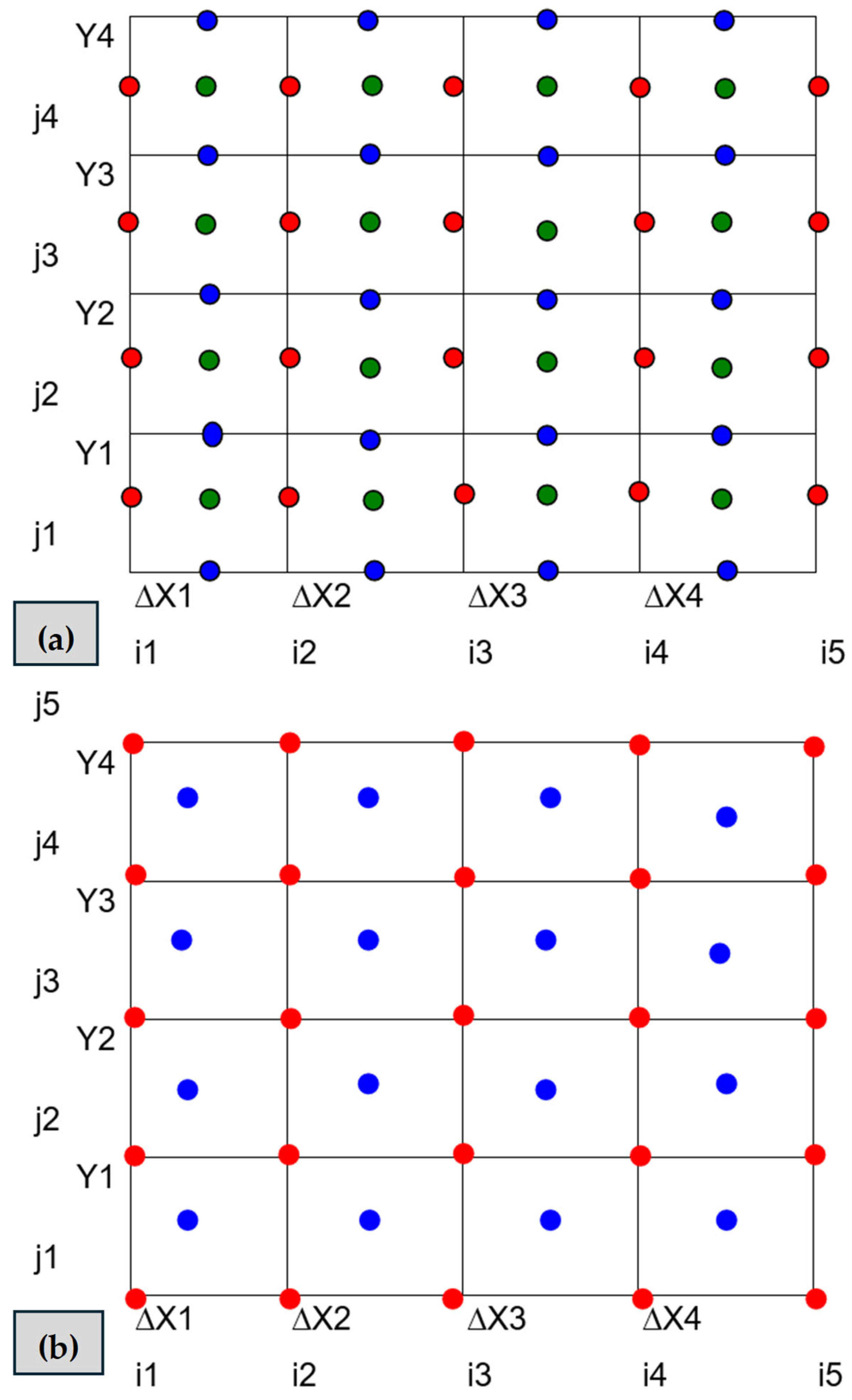
Figure A3.
Scheme for water-level estimation.
References
- Armandei, M.; Linhoss, A.C.; Camacho, R.A. Hydrodynamic Modeling of the Western Mississippi Sound Using a Linked Model System. Reg. Stud. Mar. Sci. 2021, 44, 101685. [Google Scholar] [CrossRef] [Scilit]
- Dronkers, J.J. Tidal Computations in Rivers and Coastal Waters; North-Holland Publishing Company: Amsterdam, The Netherlands, 1964. [Google Scholar]
- Coastal Engineering Research Center (USA). Shore Protection Manual; USA Army Coastal Engineering Research Center: San Francisco, CA, USA, 1973; Volume 1. [Google Scholar]
- Ozturk, M.; Yuksel, Y. Tidal and Non-Tidal Sea Level Analysis in Enclosed and Inland Basins: The Black, Aegean, Marmara, and Eastern Mediterranean (Levantine) Seas. Reg. Stud. Mar. Sci. 2023, 61, 102848. [Google Scholar] [CrossRef] [Scilit]
- Leendertse, J.J. Aspects of a Computational Model for Long-Period Water-Wave Propagation; The Rand Corporation: Santa Monica, CA, USA, 1967. [Google Scholar]
- Toro, F. A Two Dimensional Finite Element Model for Coastal Hydrodynamic Simulation. Ph.D. Thesis, University of Mississippi, Jackson, MS, USA, 1985. [Google Scholar]
- Marín, S.; Toro, F.M. Modelamiento Matemático de Fenómenos Hidrodinámicos En Regiones Cercanas a La Costa. Revista Avances en Recur. Hidraúlicos 1991, 49–61. [Google Scholar]
- Habib, M.A.; Zarillo, G.A. Construction of a Real-Time Forecast Model with Deep Learning Techniques for Coastal Engineering and Processes: Nested in a Basin Scale Suite of Models. J. Mar. Sci. Eng. 2024, 12, 1152. [Google Scholar] [CrossRef] [Scilit]
- García, M.A. Contribución Al Estudio De La Circulación Marina Mediante El Método De Los Elementos Finitos: Aplicación Al Área Del Delta Del Ebro Y Al Golfo De St. Jordi. Ph.D. Thesis, Universidad Politécnica de Cataluña, Barcelona, Spain, 1990. [Google Scholar]
- Morozov, E.G.; Frey, D.I.; Salyuk, P.A.; Budyansky, M.V. Amazon River Plume in the Western Tropical North Atlantic. J. Mar. Sci. Eng. 2024, 12, 851. [Google Scholar] [CrossRef] [Scilit]
- Kim, D.H.; Hwang, J.H.; Jeong, J.; Hong, Y.; Lee, M. Comprehensive Modeling from Watersheds to a Bay and Its Validation with Radar, Drifters, and MVP Methods. Reg. Stud. Mar. Sci. 2023, 68, 103262. [Google Scholar] [CrossRef] [Scilit]
- Speer, P.E.; Aubrey, D.G. A Study of Non-Linear Tidal Propagation in Shallow Inlet/Estuarine Systems Part II: Theory. Estuar. Coast. Shelf Sci. 1985, 21, 207–224. [Google Scholar] [CrossRef] [Scilit]
- Arrieta-Pastrana, A.; Coronado-Hernández, O.E.; Fuertes-Miquel, V.S. Analysis of the Impact of Hydraulic Gates on a Stabilized Tidal Inlet Structure: Mathematical Model and Data Measurements. Hydrology 2024, 11, 46. [Google Scholar] [CrossRef] [Scilit]
- Hill, A.E. Fortnightly Tides in a Lagoon With Variable Choking. Estuar. Coast. Shelf Sci. 1994, 38, 423–434. [Google Scholar] [CrossRef] [Scilit]
- Glorioso, P.D.; Davies, A.M. The Influence of Eddy Viscosity Formulation, Bottom Topography, and Wind Wave Effects upon the Circulation of a Shallow Bay. J. Phys. Oceanogr. 1995, 25, 1243–1264. [Google Scholar] [CrossRef] [Scilit]
- Martínez-Marrero, A. Estudio Sobre La Propagación De Ondas De Marea En Canales: Aplicación Al Análisis De Niveles Y Corrientes En La Plataforma De Gran Canaria. Ph.D. Thesis, Universidad de las Palmas de Gran Canarias, Las Palmas, Spain, 1995. [Google Scholar]
- Webb, D.J.; Holmes, R.M.; Spence, P.; England, M.H. Propagation of Barotropic Kelvin Waves around Antarctica. Ocean Dyn. 2022, 72, 405–419. [Google Scholar] [CrossRef] [Scilit]
- Wheless, G.H.; Valle-Levinson, A. A Modeling Study of Tidally Driven Estuarine Exchange through a Narrow Inlet onto a Sloping Shelf. J. Geophys. Res. Ocean. 1996, 101, 25675–25687. [Google Scholar] [CrossRef] [Scilit]
- Amin, M.; Flather, R.A. Calibration of a Numerical Model with a Limited Number of Tidal Constituents. Estuar. Coast. Shelf Sci. 1996, 43, 637–652. [Google Scholar] [CrossRef] [Scilit]
- Davies, A.M.; Jones, J.E.; Xing, J. Review of Recent Developments in Tidal Hydrodynamic Modeling. II: Turbulence Energy Models. J. Hydraul. Eng. 1997, 123, 293–302. [Google Scholar] [CrossRef] [Scilit]
- Ullman, D.S.; Wilson, R.E. Model Parameter Estimation from Data Assimilation Modeling: Temporal and Spatial Variability of the Bottom Drag Coefficient. J. Geophys. Res. Ocean. 1998, 103, 5531–5549. [Google Scholar] [CrossRef] [Scilit]
- Nguyen, V.T.; Vu, M.T.; Zhang, C. Numerical Investigation of Hydrodynamics and Cohesive Sediment Transport in Cua Lo and Cua Hoi Estuaries, Vietnam. J. Mar. Sci. Eng. 2021, 9, 1258. [Google Scholar] [CrossRef] [Scilit]
- Seenath, A. A New Approach for Handling Complex Morphologies in Hybrid Shoreline Evolution Models. Appl. Ocean Res. 2023, 141, 103754. [Google Scholar] [CrossRef] [Scilit]
- Group, D.H.I. Mike 21 & Mike 3 FLOW MODEL FM: Hydrodynamic and Transport Module Scientific Documentation. DHI Group Hørsholm Den. 2011. [Google Scholar]
- Dean, R.G.; Dalrymple, R.A. Water Wave Mechanics for Engineers and Scientists; World Scientific: Singapore, 1991; Volume 2. [Google Scholar] [CrossRef]
- Ji, Z.-G.; Moustafa, M.Z.; Hamrick, J. Hydrodynamic Modeling of a Large, Shallow Estuary. J. Mar. Sci. Eng. 2024, 12, 381. [Google Scholar] [CrossRef] [Scilit]
- Roelvink, D.; Reniers, A.; van Dongeren, A.; van Thiel de Vries, J.; McCall, R.; Lescinski, J. Modelling Storm Impacts on Beaches, Dunes and Barrier Islands. Coast. Eng. 2009, 56, 1133–1152. [Google Scholar] [CrossRef] [Scilit]
- Yu, H.; Weng, Z.; Chen, G.; Chen, X. Improved XBeach Model and Its Application in Coastal Beach Evolution under Wave Action. Coast. Eng. J. 2023, 65, 560–571. [Google Scholar] [CrossRef] [Scilit]
- Tang, P.; Lin, X.; Wang, W.; Zhang, H. Numerical Simulation of Hydrodynamic Performance of an Offshore Oscillating Water Column Wave Energy Converter Device. J. Mar. Sci. Eng. 2024, 12, 2289. [Google Scholar] [CrossRef] [Scilit]
- Lynett, P.J.; Kaihatu, J.M. Modeling of Coastal Waves and Hydrodynamics. In Springer Handbook of Ocean Engineering; Dhanak, M.R., Xiros, N.I., Eds.; Springer International Publishing: Cham, Switzerland, 2016; pp. 597–610. [Google Scholar] [CrossRef] [Scilit]
- Arrieta-Pastrana, A. Metodología de Simulación Hidrodinámica de Estuarios y Bahías. Ph.D. Thesis, Universidad de Cádiz, Cádiz, Spain, 2000. [Google Scholar]
- Thompson, E.F.; Leenknecht, D.A. Wind Estimation for Coastal Modeling Applications. J. Coa. Res. 1994, 10, 3. Available online: http://www.jstor.org/stable/4298258 (accessed on 17 February 2025).
- Ningsih, N.S.; Al Azhar, M. Modelling of Hydrodynamic Circulation in Benoa Bay, Bali. J. Mar. Sci. Technol. 2013, 18, 203–212. [Google Scholar] [CrossRef] [Scilit]
- Ganju, N.K.; Brush, M.J.; Rashleigh, B.; Aretxabaleta, A.L.; del Barrio, P.; Grear, J.S.; Harris, L.A.; Lake, S.J.; McCardell, G.; O’Donnell, J.; et al. Progress and Challenges in Coupled Hydrodynamic-Ecological Estuarine Modeling. Estuaries Coasts 2016, 39, 311–332. [Google Scholar] [CrossRef] [Scilit] [PubMed]
- Prandle, D.; Rahman, M. Tidal Response in Estuaries. J. Phys. Oceanogr. 1980, 10, 1552–1573. [Google Scholar] [CrossRef] [Scilit]

Disclaimer/Publisher’s Note: The statements, opinions and data contained in all publications are solely those of the individual author(s) and contributor(s) and not of MDPI and/or the editor(s). MDPI and/or the editor(s) disclaim responsibility for any injury to people or property resulting from any ideas, methods, instructions or products referred to in the content. |
© 2025 by the authors. Licensee MDPI, Basel, Switzerland. This article is an open access article distributed under the terms and conditions of the Creative Commons Attribution (CC BY) license (https://creativecommons.org/licenses/by/4.0/).