Predicting Future Flood Risks in the Face of Climate Change: A Frequency Analysis Perspective

Abstract

The frequency analysis of maximum flows represents a direct method to predict future flood risks in the face of climate change. Thus, the correct use of the tools (probability distributions and methods of estimating their parameters) necessary to carry out such analyzes is required to avoid possible negative consequences. This article presents four probability distributions from the generalized Beta families, using the L- and LH-moments method as parameter estimation. New elements are presented regarding the applicability of Dagum, Paralogistic, Inverse Paralogistic and the four-parameter Burr distributions in the flood frequency analysis. The article represents the continuation of the research carried out in the Faculty of Hydrotechnics, being part of larger and more complex research with the aim of developing a normative regarding flood frequency analysis using these methods. According to the results obtained, among the four analyzed distributions, the Burr distribution was found to be the best fit model because the theoretical values of the statistical indicators calibrated the corresponding values of the observed data. Considering the existence of more rigorous selection criteria, it is recommended to use these methods in the frequency analysis.

1. Introduction

The accurate determination of the maximum flows has the role of representing extremely important data in the design of hydrotechnical constructions as well as in the establishment of constructive and non-constructive measures to protect the areas subject to flooding, especially in the perspective of changes in the climatic conditions and the restoration of forested areas.

A direct method of determining these maximum flows with certain return periods is the frequency analysis [1,2,3,4], which can use the series of maximum annual flows or the partial series of these flows, their advantages and disadvantages being highlighted in previous materials [5].

Regardless of the analyzed series, the FFA is exclusively based on the use of statistical distributions and on various parameter estimation methods. Thus, the correct choice of probability distributions becomes particularly important.

The Gamma, the Generalized Pareto, and the GEV family distributions are some of the probability distributions that are most frequently employed in FFA or regional FFA [1,3,4,5,6,7,8]. But, in recent materials [9,10,11,12,13], other distributions and families of distributions have been introduced in FFA, such as distributions from the generalized beta family, generalized beta prime, and beta exponential [13], using the method of ordinary moments (MOM) and the L-moments method as parameter estimation.

Regarding the parameter estimation methods, the most used are the ordinary moments method (MOM), the L-moments method, the maximum likelihood method (MLE) and the least squares method (LSM). Among these, the L-moments method has received special attention, currently being one of the most popular methods, an aspect due to the advantage that this is a more robust method, which is less subject to bias and less affected by sampling variability [2,5,11,14,15,16,17].

Since 1997, Wang [18] postulated another parameter estimation method that has received a special attention, namely the higher order linear moments (LH-moments). This represents a generalization of the L-moments method, having the main advantage of assigning a lower importance to the small values of the maximum annual data series, knowing that these are not always floods. Thus, the “separation effect” stated by Matalas [1,14,19] is partially fulfilled. Since then, the LH-moments method was used for regional FFA [20,21,22,23], FFA [18,24,25,26], low-flow frequency analysis [27], and the annual maximum rainfall frequency analysis [28,29,30].

Important contributions, regarding the applicability of probability distributions using the LH-moments method, were made by Anghel and Ilinca, who presented all the elements necessary to apply a significant number of distributions from different families [31].

The relations and equations required to apply the L- and LH-moment approach to the Dagum (DG), Paralogistic (PR), Inverse Paralogistic (IPR), and four-parameter Burr (BR4) distributions are presented in this article. Table 1 summarizes all the novelty elements from this article.

Table 1. New elements of distributions.

New Elements	Distribution
Exact relationships for LH moments	DG, PR, IPR, BR4
Approximate relations for LH moments	PR, IPR
Approximate relations for L-moments	PR
LH moments diagrams and relationships	PR, IPR
Exact frequency factors	DG, PR, IPR, BR4
Approximate frequency factors	PR, IPR

The article’s primary goal is to give researchers all the tools (approximate estimates, frequency factors, frequency factor approximations, etc.) they need to use these distributions in frequency analysis in hydrology. The presented analysis refers only to the pure Statistics component and not to the component of the analysis of the physical phenomena of the formation of maximum flows (physical systems, dynamics, etc.).

All these new elements are applied on four case studies, with the aim of verifying the relationships, determining the maximum flows for the usual annual exceedance probabilities.

2. Methods

The method for estimating the parameters of the analyzed distributions is the L- and the first level LH-moments methods.

2.1. Probability Distributions

In this section, only the inverse functions of the analyzed distributions are presented (see Table 2), the L- and LH-moments are based on the inverse function. Density functions and cumulative functions can be found in others materials [13,32,33].

Table 2. The quantile functions.

Probability Distribution	$\mathbf{Quantile}\mathbf{Functions}\mathit{x}\left(\mathit{p}\right)$
Dagum	$\beta \cdot {\left({\left(1-p\right)}^{-\frac{1}{\gamma }}-1\right)}^{-\frac{1}{\alpha }}$
Burr	$\gamma +\lambda \cdot {\left(\frac{1}{{\left(\frac{1}{1-p}\right)}^{\frac{1}{\alpha }}-1}\right)}^{\frac{1}{\beta }}$
Paralogistic	$\gamma +\beta \cdot {\left(p^{-\frac{1}{\alpha }}-1\right)}^{\frac{1}{\alpha }}$
Inverse Paralogistic	$\gamma +\beta \cdot {\left(\frac{{\left(1-p\right)}^{\frac{1}{\alpha }}}{1-{\left(1-p\right)}^{\frac{1}{\alpha }}}\right)}^{\frac{1}{\alpha }}$

Considering that these inverse functions can be expressed using frequency factors [11,13], the exact and approximate relationships of these frequency factors are presented in the Supplementary File.

2.2. Determination of Distribution Parameters

This section presents the relationships for the L- and first level LH-moments. The sample L-moments and LH-moments are determined according to [1,6,7,8,9], and, respectively, [18,24].

In general, the parameters are determined by solving systems of nonlinear equations. This is also the main disadvantage in using these distributions. This obstacle is overcome by presenting approximate relationships (for PR and IPR), characterized by very small errors.

Considering that in general, the L-skewness and the LH- skewness depend on a single parameter, the latter can be approximately determined using different functions (logarithmic, rational and exponential functions).

In the next section, the relations for the exact and approximate estimation of the parameters are presented.

2.2.1. Dagum Distribution (DG)

The equations for the L-moments are:

$$L_1=\beta \cdot \frac{\mathsf{\Gamma }\left(\gamma +\frac{1}{\alpha }\right)\cdot \mathsf{\Gamma }\left(1-\frac{1}{\alpha }\right)}{\mathsf{\Gamma }\left(\gamma +1\right)}$$

(1)

$$L_2=\gamma \cdot \beta \cdot \left(2\cdot \frac{\mathsf{\Gamma }\left(2\cdot \gamma +\frac{1}{\alpha }\right)\cdot \mathsf{\Gamma }\left(1-\frac{1}{\alpha }\right)}{\mathsf{\Gamma }\left(2\cdot \gamma +1\right)}-\frac{\mathsf{\Gamma }\left(\gamma +\frac{1}{\alpha }\right)\cdot \mathsf{\Gamma }\left(1-\frac{1}{\alpha }\right)}{\mathsf{\Gamma }\left(\gamma +1\right)}\right)$$

(2)

$$L_3=\gamma \cdot \beta \cdot \left(\begin{array}{l}6\cdot \frac{\mathsf{\Gamma }\left(3\cdot \gamma +\frac{1}{\alpha }\right)\cdot \mathsf{\Gamma }\left(1-\frac{1}{\alpha }\right)}{\mathsf{\Gamma }\left(3\cdot \gamma +1\right)}-6\cdot \frac{\mathsf{\Gamma }\left(2\cdot \gamma +\frac{1}{\alpha }\right)\cdot \mathsf{\Gamma }\left(1-\frac{1}{\alpha }\right)}{\mathsf{\Gamma }\left(2\cdot \gamma +1\right)}+\\ \frac{\mathsf{\Gamma }\left(\gamma +\frac{1}{\alpha }\right)\cdot \mathsf{\Gamma }\left(1-\frac{1}{\alpha }\right)}{\mathsf{\Gamma }\left(\gamma +1\right)}\end{array}\right)$$

(3)

where, $L_1,L_2$ and $L_3$ represent the first three linear moments; $\alpha$ and $\gamma$ are the shape parameters; $\beta$ is the scale parameter.

The following equations apply to the first level LH-moments:

$$L_{H1}=\beta \cdot \frac{\mathsf{\Gamma }\left(2\cdot \gamma +\frac{1}{\alpha }\right)\cdot \mathsf{\Gamma }\left(1-\frac{1}{\alpha }\right)}{\mathsf{\Gamma }\left(2\cdot \gamma \right)}$$

(4)

$$L_{H2}=\frac{3}{2}\cdot \beta \cdot \mathsf{\Gamma }\left(1-\frac{1}{\alpha }\right)\cdot \left(\frac{\mathsf{\Gamma }\left(3\cdot \gamma +\frac{1}{\alpha }\right)}{\mathsf{\Gamma }\left(3\cdot \gamma \right)}-\frac{\mathsf{\Gamma }\left(2\cdot \gamma +\frac{1}{\alpha }\right)}{\mathsf{\Gamma }\left(2\cdot \gamma \right)}\right)$$

(5)

$$L_{H3}=4\cdot \beta \cdot \mathsf{\Gamma }\left(1-\frac{1}{\alpha }\right)\cdot \left(5\cdot \frac{\mathsf{\Gamma }\left(4\cdot \gamma +\frac{1}{\alpha }\right)}{6\cdot \mathsf{\Gamma }\left(4\cdot \gamma \right)}-\frac{4\cdot \mathsf{\Gamma }\left(3\cdot \gamma +\frac{1}{\alpha }\right)}{3\cdot \mathsf{\Gamma }\left(3\cdot \gamma \right)}+\frac{\mathsf{\Gamma }\left(2\cdot \gamma +\frac{1}{\alpha }\right)}{2\cdot \mathsf{\Gamma }\left(2\cdot \gamma \right)}\right)$$

(6)

where, $L_{H1},L_{H2}$ and $L_{H3}$ represent the first three high-order linear moments.

2.2.2. Paralogistic Distribution (PR)

The linear moments are:

$$L_1=\gamma +\frac{\beta \cdot \mathsf{\Gamma }\left(1+\frac{1}{\alpha }\right)\cdot \mathsf{\Gamma }\left(\alpha -\frac{1}{\alpha }\right)}{\mathsf{\Gamma }\left(\alpha \right)}$$

(7)

$$L_2=\beta \cdot \mathsf{\Gamma }\left(1+\frac{1}{\alpha }\right)\cdot \left(\frac{\mathsf{\Gamma }\left(\alpha -\frac{1}{\alpha }\right)}{\mathsf{\Gamma }\left(\alpha \right)}-\frac{\mathsf{\Gamma }\left(2\cdot \alpha -\frac{1}{\alpha }\right)}{\mathsf{\Gamma }\left(2\cdot \alpha \right)}\right)$$

(8)

$$L_3=\beta \cdot \mathsf{\Gamma }\left(1+\frac{1}{\alpha }\right)\cdot \left(\frac{\mathsf{\Gamma }\left(\alpha -\frac{1}{\alpha }\right)}{\mathsf{\Gamma }\left(\alpha \right)}+\frac{2\cdot \mathsf{\Gamma }\left(3\cdot \alpha -\frac{1}{\alpha }\right)}{\mathsf{\Gamma }\left(3\cdot \alpha \right)}-\frac{3\cdot \mathsf{\Gamma }\left(2\cdot \alpha -\frac{1}{\alpha }\right)}{\mathsf{\Gamma }\left(2\cdot \alpha \right)}\right)$$

(9)

where, $\alpha ,\beta$ and $\gamma$ are the shape, the scale and the position parameters.

For the parameter $\alpha$, the following approximation can be used:

$$\alpha =\exp \left(\begin{array}{l}0.000006321-0.499775727\cdot \ln \left({\tau }_3\right)+0.126690856\cdot \ln {\left({\tau }_3\right)}^2+\\ 0.067638333\cdot \ln {\left({\tau }_3\right)}^3+0.002255123\cdot \ln {\left({\tau }_3\right)}^4-0.00279206\cdot \ln {\left({\tau }_3\right)}^5-\\ 0.000477164\cdot \ln {\left({\tau }_3\right)}^6-0.000016444\cdot \ln {\left({\tau }_3\right)}^7+0.000001032\cdot \ln {\left({\tau }_3\right)}^8\end{array}\right)$$

(10)

$$\beta =\frac{L_2\cdot \alpha }{\mathsf{\Gamma }\left(\frac{1}{\alpha }\right)\cdot \left(\frac{\mathsf{\Gamma }\left(\alpha -\frac{1}{\alpha }\right)}{\mathsf{\Gamma }\left(\alpha \right)}-\frac{\mathsf{\Gamma }\left(2\cdot \alpha -\frac{1}{\alpha }\right)}{\mathsf{\Gamma }\left(2\cdot \alpha \right)}\right)}$$

(11)

$$\gamma =L_1-\frac{\beta \cdot \mathsf{\Gamma }\left(1+\frac{1}{\alpha }\right)\cdot \mathsf{\Gamma }\left(\alpha -\frac{1}{\alpha }\right)}{\mathsf{\Gamma }\left(\alpha \right)}$$

(12)

where, ${\tau }_3=\raisebox{1ex}{$L_3$}\!\left/ \!\raisebox{-1ex}{$L_2$}\right.$ is the L-skewness.

The linear moments for the first level LH-moments are as follows:

$$L_{H1}=\gamma +\frac{\beta }{\alpha }\cdot \mathsf{\Gamma }\left(\frac{1}{\alpha }\right)\cdot \left(\frac{2\cdot \mathsf{\Gamma }\left(\alpha -\frac{1}{\alpha }\right)}{\mathsf{\Gamma }\left(\alpha \right)}-\frac{\mathsf{\Gamma }\left(2\cdot \alpha -\frac{1}{\alpha }\right)}{\mathsf{\Gamma }\left(2\cdot \alpha \right)}\right)$$

(13)

$$L_{H2}=\frac{3\cdot \beta }{\alpha }\cdot \mathsf{\Gamma }\left(\frac{1}{\alpha }\right)\cdot \left(\frac{\mathsf{\Gamma }\left(3\cdot \alpha -\frac{1}{\alpha }\right)}{2\cdot \mathsf{\Gamma }\left(3\cdot \alpha \right)}-\frac{\mathsf{\Gamma }\left(2\cdot \alpha -\frac{1}{\alpha }\right)}{\mathsf{\Gamma }\left(2\cdot \alpha \right)}+\frac{\mathsf{\Gamma }\left(\alpha -\frac{1}{\alpha }\right)}{2\cdot \mathsf{\Gamma }\left(\alpha \right)}\right)$$

(14)

$$L_{H3}=\frac{2\cdot \beta }{\alpha }\cdot \mathsf{\Gamma }\left(\frac{1}{\alpha }\right)\cdot \left(\frac{4\cdot \mathsf{\Gamma }\left(3\cdot \alpha -\frac{1}{\alpha }\right)}{\mathsf{\Gamma }\left(3\cdot \alpha \right)}-\frac{5\cdot \mathsf{\Gamma }\left(4\cdot \alpha -\frac{1}{\alpha }\right)}{3\cdot \mathsf{\Gamma }\left(4\cdot \alpha \right)}-\frac{3\cdot \mathsf{\Gamma }\left(2\cdot \alpha -\frac{1}{\alpha }\right)}{\mathsf{\Gamma }\left(2\cdot \alpha \right)}+\frac{2\cdot \mathsf{\Gamma }\left(\alpha -\frac{1}{\alpha }\right)}{3\cdot \mathsf{\Gamma }\left(\alpha \right)}\right)$$

(15)

The parameter $\alpha$ can be estimated, using a rational function ($0.1<{\tau }_{H3}<0.88$):

$$\alpha =\frac{30.67728772+43.85465205\cdot {\tau }_{H3}+17.39998218\cdot {\tau }_{H3}{}^2+4.59707366\cdot {\tau }_{H3}{}^3}{1+48.74542611\cdot {\tau }_{H3}+53.51830483\cdot {\tau }_{H3}{}^2}$$

(16)

$$\beta =\frac{L_{H2}}{\frac{3}{\alpha }\cdot \mathsf{\Gamma }\left(\frac{1}{\alpha }\right)\cdot \left(\frac{\mathsf{\Gamma }\left(3\cdot \alpha -\frac{1}{\alpha }\right)}{2\cdot \mathsf{\Gamma }\left(3\cdot \alpha \right)}-\frac{\mathsf{\Gamma }\left(2\cdot \alpha -\frac{1}{\alpha }\right)}{\mathsf{\Gamma }\left(2\cdot \alpha \right)}+\frac{\mathsf{\Gamma }\left(\alpha -\frac{1}{\alpha }\right)}{2\cdot \mathsf{\Gamma }\left(\alpha \right)}\right)}$$

(17)

$$\gamma =L_{H1}-\frac{\beta \cdot \mathsf{\Gamma }\left(\frac{1}{\alpha }\right)}{\alpha }\cdot \left(\frac{2\cdot \mathsf{\Gamma }\left(\alpha -\frac{1}{\alpha }\right)}{\mathsf{\Gamma }\left(\alpha \right)}-\frac{\mathsf{\Gamma }\left(2\cdot \alpha -\frac{1}{\alpha }\right)}{\mathsf{\Gamma }\left(2\cdot \alpha \right)}\right)$$

(18)

where, ${\tau }_{H3}=\raisebox{1ex}{$L_{H3}$}\!\left/ \!\raisebox{-1ex}{$L_{H2}$}\right.$ is the LH-skewness.

2.2.3. Inverse Paralogistic (IPR)

The equations for the L-moments are:

$$L_1=\gamma +\frac{\beta \cdot \mathsf{\Gamma }\left(\frac{1}{\alpha }+\alpha \right)\cdot \mathsf{\Gamma }\left(1-\frac{1}{\alpha }\right)}{\mathsf{\Gamma }\left(\alpha \right)}$$

(19)

$$L_2=\beta \cdot \mathsf{\Gamma }\left(1-\frac{1}{\alpha }\right)\cdot \left(\frac{\mathsf{\Gamma }\left(\frac{1}{\alpha }+2\cdot \alpha \right)}{\mathsf{\Gamma }\left(2\cdot \alpha \right)}-\frac{\mathsf{\Gamma }\left(\frac{1}{\alpha }+\alpha \right)}{\mathsf{\Gamma }\left(\alpha \right)}\right)$$

(20)

$$L_3=\beta \cdot \mathsf{\Gamma }\left(1-\frac{1}{\alpha }\right)\cdot \left(\frac{\mathsf{\Gamma }\left(\alpha +\frac{1}{\alpha }\right)}{\mathsf{\Gamma }\left(\alpha \right)}+\frac{2\cdot \mathsf{\Gamma }\left(3\cdot \alpha +\frac{1}{\alpha }\right)}{\mathsf{\Gamma }\left(3\cdot \alpha \right)}-\frac{3\cdot \mathsf{\Gamma }\left(2\cdot \alpha +\frac{1}{\alpha }\right)}{\mathsf{\Gamma }\left(2\cdot \alpha \right)}\right)$$

(21)

where, $\alpha ,\beta$ and $\gamma$ are the shape, the scale and the position parameters.

An approximate form for parameter $\alpha$ can be adopted:

If $0.17\le {\tau }_3\le \frac{1}{3}$:

$$\alpha =\frac{5.07675\cdot {10}^3-7.55684\cdot {10}^4\cdot {\tau }_3+5.36797\cdot {10}^5\cdot {\tau }_3^2-1.35970\cdot {10}^6\cdot {\tau }_3^3+1.30233\cdot {10}^6\cdot {\tau }_3^4}{1-4.59437\cdot {10}^3\cdot {\tau }_3+2.70167\cdot {10}^4\cdot {\tau }_3^2}$$

(22)

If $\frac{1}{3}<{\tau }_3<1$:

$$\begin{array}{l}\alpha =5.37952\cdot 10-4.84016\cdot {10}^2\cdot {\tau }_3+2.02215\cdot {10}^3\cdot {\tau }_3^2-4.79644\cdot {10}^3\cdot {\tau }_3^3+\\ 6.86370\cdot {10}^3\cdot {\tau }_3^4-5.88301\cdot {10}^3\cdot {\tau }_3^5+2.78592\cdot {10}^3\cdot {\tau }_3^6-5.61108\cdot {10}^2\cdot {\tau }_3^7\end{array}$$

(23)

$$\beta =\frac{L_2}{\mathsf{\Gamma }\left(1-\frac{1}{\alpha }\right)\cdot \left(\frac{\mathsf{\Gamma }\left(\frac{1}{\alpha }+2\cdot \alpha \right)}{\mathsf{\Gamma }\left(2\cdot \alpha \right)}-\frac{\mathsf{\Gamma }\left(\frac{1}{\alpha }+\alpha \right)}{\mathsf{\Gamma }\left(\alpha \right)}\right)}$$

(24)

$$\gamma =L_1-\frac{\beta \cdot \mathsf{\Gamma }\left(\frac{1}{\alpha }+\alpha \right)\cdot \mathsf{\Gamma }\left(1-\frac{1}{\alpha }\right)}{\mathsf{\Gamma }\left(\alpha \right)}$$

(25)

For the first level LH-moments, the equations are:

$$L_{H1}=\gamma +\beta \cdot \frac{\mathsf{\Gamma }\left(2\cdot \alpha +\frac{1}{\alpha }\right)\left(1-\frac{1}{\alpha }\right)}{\mathsf{\Gamma }\left(2\cdot \alpha \right)}$$

(26)

$$L_{H2}=\frac{3\cdot \beta }{2}\cdot \mathsf{\Gamma }\left(1-\frac{1}{\alpha }\right)\cdot \left(\frac{\mathsf{\Gamma }\left(3\cdot \alpha +\frac{1}{\alpha }\right)}{\mathsf{\Gamma }\left(3\cdot \alpha \right)}-\frac{\mathsf{\Gamma }\left(2\cdot \alpha +\frac{1}{\alpha }\right)}{\mathsf{\Gamma }\left(2\cdot \alpha \right)}\right)$$

(27)

$$L_{H3}=2\cdot \beta \cdot \mathsf{\Gamma }\left(1-\frac{1}{\alpha }\right)\cdot \left(\frac{5\cdot \mathsf{\Gamma }\left(4\cdot \alpha +\frac{1}{\alpha }\right)}{3\cdot \mathsf{\Gamma }\left(4\cdot \alpha \right)}-\frac{8\cdot \mathsf{\Gamma }\left(3\cdot \alpha +\frac{1}{\alpha }\right)}{3\cdot \mathsf{\Gamma }\left(3\cdot \alpha \right)}+\frac{\mathsf{\Gamma }\left(2\cdot \alpha +\frac{1}{\alpha }\right)}{\mathsf{\Gamma }\left(2\cdot \alpha \right)}\right)$$

(28)

An approximate form for parameter $\alpha$ can be adopted:

If $0.25\le {\tau }_{H3}\le 1/3$:

$$\alpha =\frac{16517.60198-82738.36913\cdot {\tau }_{H3}+644148.00047\cdot {\tau }_{H3}{}^2-645765.89383\cdot {\tau }_{H3}{}^3}{1-54573.65663\cdot {\tau }_{H3}+224419.26179\cdot {\tau }_{H3}{}^2}$$

(29)

If $1/3<{\tau }_{H3}<89$:

$$\alpha =\frac{5.9986867-60.4311085\cdot {\tau }_{H3}-29.7201729\cdot {\tau }_{H3}{}^2}{1+18.5442652\cdot {\tau }_{H3}-81.3230745\cdot {\tau }_{H3}{}^2-35.3549804\cdot {\tau }_{H3}{}^3}$$

(30)

$$\beta =\frac{L_{H2}}{\frac{3}{2}\cdot \mathsf{\Gamma }\left(1-\frac{1}{\alpha }\right)\cdot \left(\frac{\mathsf{\Gamma }\left(\frac{1}{\alpha }+3\cdot \alpha \right)}{\mathsf{\Gamma }\left(3\cdot \alpha \right)}-\frac{\mathsf{\Gamma }\left(\frac{1}{\alpha }+2\cdot \alpha \right)}{\mathsf{\Gamma }\left(2\cdot \alpha \right)}\right)}$$

(31)

$$\gamma =L_{H1}-\frac{\beta \cdot \mathsf{\Gamma }\left(\frac{1}{\alpha }+2\cdot \alpha \right)\cdot \mathsf{\Gamma }\left(1-\frac{1}{\alpha }\right)}{\mathsf{\Gamma }\left(2\cdot \alpha \right)}$$

(32)

2.2.4. The Four Parameters Burr Distribution (BR4)

For the L-moments, the equations are:

$$L_1=\gamma +\frac{\lambda \cdot \mathsf{\Gamma }\left(1-\frac{1}{\beta }\right)\cdot \mathsf{\Gamma }\left(\alpha +\frac{1}{\beta }\right)}{\mathsf{\Gamma }\left(\alpha \right)}$$

(33)

$$L_2=\lambda \cdot \mathsf{\Gamma }\left(1-\frac{1}{\beta }\right)\cdot \left(\frac{\mathsf{\Gamma }\left(2\cdot \alpha +\frac{1}{\beta }\right)}{\mathsf{\Gamma }\left(2\cdot \alpha \right)}-\frac{\mathsf{\Gamma }\left(\alpha +\frac{1}{\beta }\right)}{\mathsf{\Gamma }\left(\alpha \right)}\right)$$

(34)

$$L_3=\lambda \cdot \mathsf{\Gamma }\left(1-\frac{1}{\beta }\right)\cdot \left(\frac{2\cdot \mathsf{\Gamma }\left(3\cdot \alpha +\frac{1}{\beta }\right)}{\mathsf{\Gamma }\left(3\cdot \alpha \right)}-\frac{3\cdot \mathsf{\Gamma }\left(2\cdot \alpha +\frac{1}{\beta }\right)}{\mathsf{\Gamma }\left(2\cdot \alpha \right)}+\frac{\mathsf{\Gamma }\left(\alpha +\frac{1}{\beta }\right)}{\mathsf{\Gamma }\left(\alpha \right)}\right)$$

(35)

$$L_3=\lambda \cdot \mathsf{\Gamma }\left(1-\frac{1}{\beta }\right)\cdot \left(\frac{5\cdot \mathsf{\Gamma }\left(4\cdot \alpha +\frac{1}{\beta }\right)}{\mathsf{\Gamma }\left(4\cdot \alpha \right)}-\frac{10\cdot \mathsf{\Gamma }\left(3\cdot \alpha +\frac{1}{\beta }\right)}{\mathsf{\Gamma }\left(3\cdot \alpha \right)}+\frac{6\cdot \mathsf{\Gamma }\left(2\cdot \alpha +\frac{1}{\beta }\right)}{\mathsf{\Gamma }\left(2\cdot \alpha \right)}-\frac{\mathsf{\Gamma }\left(\alpha +\frac{1}{\beta }\right)}{\mathsf{\Gamma }\left(\alpha \right)}\right)$$

(36)

where, $\alpha$ and $\beta$ are the shape parameters; $\lambda$ is the scale parameter; $\gamma$ is the position parameter.

The equations for the first level LH-moments are:

$$L_{H1}=\gamma +\frac{\lambda \cdot \mathsf{\Gamma }\left(1-\frac{1}{\beta }\right)\cdot \mathsf{\Gamma }\left(2\cdot \alpha +\frac{1}{\beta }\right)}{\mathsf{\Gamma }\left(2\cdot \alpha \right)}$$

(37)

$$L_{H2}=\frac{3}{2}\cdot \lambda \cdot \mathsf{\Gamma }\left(1-\frac{1}{\beta }\right)\cdot \left(\frac{\mathsf{\Gamma }\left(3\cdot \alpha +\frac{1}{\beta }\right)}{\mathsf{\Gamma }\left(3\cdot \alpha \right)}-\frac{\mathsf{\Gamma }\left(2\cdot \alpha +\frac{1}{\beta }\right)}{\mathsf{\Gamma }\left(2\cdot \alpha \right)}\right)$$

(38)

$$L_{H3}=2\cdot \lambda \cdot \mathsf{\Gamma }\left(1-\frac{1}{\beta }\right)\cdot \left(\frac{5\cdot \mathsf{\Gamma }\left(4\cdot \alpha +\frac{1}{\beta }\right)}{3\cdot \mathsf{\Gamma }\left(4\cdot \alpha \right)}-\frac{8\cdot \mathsf{\Gamma }\left(3\cdot \alpha +\frac{1}{\beta }\right)}{3\cdot \mathsf{\Gamma }\left(3\cdot \alpha \right)}+\frac{\mathsf{\Gamma }\left(2\cdot \alpha +\frac{1}{\beta }\right)}{\mathsf{\Gamma }\left(2\cdot \alpha \right)}\right)$$

(39)

$$L_{H4}=\frac{5}{2}\cdot \lambda \cdot \mathsf{\Gamma }\left(1-\frac{1}{\beta }\right)\cdot \left(\frac{21\cdot \mathsf{\Gamma }\left(5\cdot \alpha +\frac{1}{\beta }\right)}{6\cdot \mathsf{\Gamma }\left(5\cdot \alpha \right)}-\frac{15\cdot \mathsf{\Gamma }\left(4\cdot \alpha +\frac{1}{\beta }\right)}{2\cdot \mathsf{\Gamma }\left(4\cdot \alpha \right)}+\frac{5\cdot \mathsf{\Gamma }\left(3\cdot \alpha +\frac{1}{\beta }\right)}{\mathsf{\Gamma }\left(3\cdot \alpha \right)}-\frac{\mathsf{\Gamma }\left(2\cdot \alpha +\frac{1}{\beta }\right)}{\mathsf{\Gamma }\left(2\cdot \alpha \right)}\right)$$

(40)

3. Case Studies

The case studies consist in determining the maximum flows with the annual exceedance probabilities of 0.01%, 0.1%, 0.5%, 1%, 40% and 80%, on the Jijia, Buhai, Miletin and Sitna Rivers from the Prut River basin, Romania.

The Jijia river is a tributary of the Prut River, originating from the Hiliseu-Horia locality, Botosani. The rivers Buhai, Miletin and Sitna are part of the hydrographic basin of the River Jijia, being its right tributaries [34].

The analyzed rivers are located in the eastern part of Romania with a general northeast orientation, as shown in Figure 1 (47°55′59.6″ N 26°24′17.1″ E).

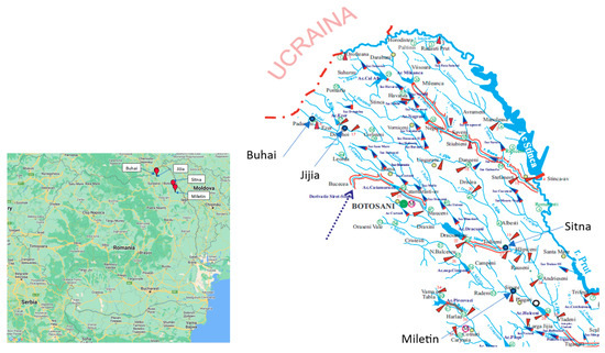
Figure 1. The positioning of the rivers: Jijia, Buhai, Miletin and Sitna; and the positioning of the hydrometric stations: Dorohoi, Padureni, Sipote and Todireni.

The Prut River has its sources in the Wooded Carpathians (Ukraine); its length on the territory of Romania is 742 km; and it has a hydrographic basin of 10,990 km², representing about 4.6% of Romania’s surface [34].

A temperate continental climate characterizes the Prut-Barlad hydrographic space. In terms of thermal regime and precipitation, a multiannual average temperature of 9.0 °C and multiannual average precipitation quantities ranging from 400 mm to 600 mm per year are reported. From a geological perspective, siliceous features dominate the landscape of the analyzed river’s watershed.

The morphometric elements of the four analyzed rivers are presented centrally in Table 3 [34].

Table 3. The morphometric elements for the analyzed rivers.

River	Length [km]	Average Stream Slope [‰]	Sinuosity Coefficient [-]	Average Altitude, [m]	Catchments Area, [km2]
Jijia	275	1.0	1.45	152	5757
Buhai	18	10	1.17	279	134
Miletin	90	3.0	1.24	166	675
Sitna	78	2.0	1.4	166	943

The four monitoring stations are positioned so that the regime of maximum recorded flows is a natural one. Appendix A presents a tabular and graphical series of the maximum yearly flows recorded at each of the four stations over time. The analysis period varies between 37 years (the Buhai and Miletin Rivers) and 57 years (the Jijia and Sitna Rivers).

The statistical indicators specific to these recorded data are presented in Table 4.

Table 4. The statistical indicators for the analyzed rivers.

River	MOM		L-Moments Method							LH-Moments Method
	$\mathit{\mu }$	${\mathit{C}}_{\mathit{v}}$	${\mathit{L}}_1$	${\mathit{L}}_2$	${\mathit{L}}_3$	${\mathit{L}}_4$	${\mathit{\tau }}_2$	${\mathit{\tau }}_3$	${\mathit{\tau }}_4$	${\mathit{L}}_{\mathit{H}1}$	${\mathit{L}}_{\mathit{H}2}$	${\mathit{L}}_{\mathit{H}3}$	${\mathit{L}}_{\mathit{H}4}$	${\mathit{\tau }}_{\mathit{H}2}$	${\mathit{\tau }}_{\mathit{H}3}$	${\mathit{\tau }}_{\mathit{H}4}$
	[m3/s]	[-]	[m3/s]	[m3/s]	[m3/s]	[m3/s]	[-]	[-]	[-]	[m3/s]	[m3/s]	[m3/s]	[m3/s]	[-]	[-]	[-]
Jijia	32.1	1.22	32.1	18.3	8.22	4.47	0.5703	0.4483	0.2436	50.5	19.9	8.46	4.59	0.3945	0.4247	0.2307
Buhai	14.4	1.452	14.4	8.78	4.93	3.28	0.6102	0.5607	0.3731	23.2	10.3	5.47	3.40	0.4436	0.5319	0.3303
Miletin	42.5	0.883	42.5	18.1	5.52	4.89	0.264	0.3041	0.2698	60.7	17.8	6.94	5.63	0.2924	0.3912	0.3175
Sitna	53.9	0.931	53.9	24.3	8.53	5.96	0.4508	0.3513	0.2451	78.2	24.6	9.66	6.15	0.3149	0.3923	0.2496

Notes: $\mu$ and $C_v$ represents the arithmetic mean and the coefficient of variation; $L_1,L_2,L_3$ and $L_4$ represents the first four L-moments; ${\tau }_2,{\tau }_3$ and ${\tau }_4$ represents the coefficient of L-variation, L-skewness and L-kurtosis. Analyzing the values of the coefficient of variation, we can observe an average torrentiality, with the exception of the Buhai river with a more pronounced torrentiality.

Considering that the first stage consists of checking the homogeneity of the data as well as identifying the possible outliers, the testing of these two conditions was carried out with the help of the von Neumann and Grubb-Beck tests with a confidence level of 10%. No extreme values were identified, and the analyzed data are homogeneous (see Table 5).

Table 5. Results of statistical tests for homogeneity and outliers.

River	Homogeneity	Outliers	Qmax for the Observed Data
	von Newman	Grubb-Beck
	[-]	[m3/s]	[m3/s]
Jijia	2.0712	548	190
Buhai	2.3503	159	96
Miletin	2.1681	353	204
Sitna	2.4471	507	290

4. Results and Discussions

In general, FFA involves the determination of maximum flows, regardless of the length of the analyzed data series, for the annual exceedance probabilities corresponding to rare and very rare events (the flow with a return period of 10,000 years, the value used in the design of hydrotechnical dam-type retention constructions—First class of importance, Category A). It is important that the values are characterized by as small as possible errors and uncertainties, depending (from a statistical point of view) on the statistical distributions and the method of estimating the parameters used.

The four analyzed probability distributions were applied to determine the maximum flows on the Jijia, Buhai, Miletin and Sitna Rivers, using the L- and first order LH-moments methods, as parameter estimation methods.

In the analysis, the annual maximum flow series (AMS) was used, its main advantage being the ease of data selection, the data which represents the maximum flows characteristic of each year of analysis (block maxima). The major disadvantage is the fact that the lower maximum values do not, in many cases, also represent floods. There are values higher than this in the chronological series of maximum flows, which naturally should be taken into consideration, but whose selection requires additional and often difficult operations. This principle is the basis of the analysis with partial series, both Peak Over Threshold (POT) [35,36,37,38] and Annual Exceedance Series (AES) [39,40]. A similar principle is also the basis of the LH-moments method, by reducing the importance of the lower maximum flows.

4.1. Estimated Parameters and Quantiles

The resulting values of the parameters are summarized in Table 6. Their presentation is necessary so that the results can be reproduced, thus ensuring the objectivity of the analysis.

Table 6. Estimated parameters using L-moments and LH-moments.

Parameter	Distribution
	DG	PR	IPR	BR4	DG	PR	IPR	BR4
	L-Moments				LH-Moments (First Level)
	Jijia River
$\alpha$	2.3353	1.5672	2.3426	0.1799	2.5609	1.6837	2.9441	0.1437
$\beta$	48.1	34.5	22.7	2.6613	59.0	43.8	35.0	2.8001
$\gamma$	0.3093	−4.27	−16.1	2.32	0.2334	−9.86	−35.1	3.95
$\lambda$	-	-	-	66.6	-	-	-	74.6
	Bahna River
$\alpha$	1.798	1.3757	1.8029	0.2621	1.906	1.4172	1.9788	0.1528
$\beta$	12.1	10.3	6.57	1.9499	16.2	11.9	8.2	2.1129
$\gamma$	0.5647	−0.298	−2.56	1.34	0.3994	−1.345	−5.34	2.67
$\lambda$	-	-	-	20.7	-	-	-	30.1
	Miletin River
$\alpha$	3.1175	1.9546	4.2066	1.0611	2.8317	1.7967	3.5184	0.761
$\beta$	57.5	58.9	56.7	3.2033	46.8	47.3	42.4	2.6568
$\gamma$	0.3811	−4.56	−51.8	−16.34	0.5509	2.12	−31.99	0.25
$\lambda$	-	-	-	48.7	-	-	-	38.8
	Sitna River
$\alpha$	2.7591	1.8033	3.297	22.676	2.7679	1.7925	3.4943	5.3107
$\beta$	66.5	66.3	52.7	3.7366	67.0	65.2	58.2	3.5955
$\gamma$	0.4376	−3.47	−41.6	−63.8	0.4323	−2.83	−49.5	−55.3
$\lambda$	-	-	-	41.0	-	-	-	55.2

The values of the derived quantiles are displayed in Table 7 using the two parameter estimation methods. The quantile values are presented only for the annual exceedance probabilities interested in flood frequency analysis, namely for rare events (left-hand, upper part of the graph) where, in most cases, there are no recorded data.

Table 7. Estimated flood discharge (m³/s), for 0.01%, 0.1%, 0.5%, 1%, 40% and 80%.

Distribution	Annual Exceedance Probabilities [%]
	L-Moments Method						LH-Moments (First Level)
	0.01	0.1	0.5	1	40	80	0.01	0.1	0.5	1	40	80
	Jijia River
DG	1503	560	280	207	26.0	5.20	1219	496	263	199	26.3	4.0
PR	1460	566	287	213	25.5	6.14	1117	487	267	204	26.3	3.89
IPR	1652	608	297	217	25.5	6.76	1118	492	270	206	26.4	3.86
BR4	1116	471	257	197	25.8	4.63	1005	443	250	195	25.1	5.32
	Buhai River
DG	1471	409	166	113	9.72	2.55	1257	375	161	111	9.84	1.98
PR	1337	394	166	114	9.60	2.62	1160	366	162	113	9.74	2.06
IPR	1505	418	169	114	9.65	2.81	1211	374	163	113	9.86	1.96
BR4	1176	362	158	111	9.60	2.23	968	327	153	110	8.95	2.87
	Miletin River
DG	810	387	230	184	41.2	14.9	981	435	246	192	40.3	17.0
PR	649	349	223	182	40.1	15.4	820	399	239	191	39.8	17.5
IPR	660	360	229	186	40.4	16.1	799	400	241	192	39.9	17.5
BR4	863	412	242	192	40.2	16.4	1122	471	257	198	39.7	18.6
	Sitna River
DG	1388	602	335	260	49.9	17.7	1379	600	335	260	49.9	17.6
PR	1119	545	325	258	49.3	18.1	1140	550	327	259	49.2	18.3
IPR	1195	574	336	264	49.0	19.1	1112	551	329	261	49.3	18.4
BR4	1049	537	326	260	49.1	18.7	1083	545	328	261	49.2	18.4

In general, all these annual exceedance probabilities are used for the design of important hydrotechnical constructions, especially dams for water storage and for bankfull discharge. For high annual exceedance probabilities (>80%), the values are not of interest in the analysis of maximum flows.

Figure 2, Figure 3, Figure 4 and Figure 5 show the fitting models of the four analyzed rivers. The Hazen empirical probability was used [1,3,4,41]. In general, for the L-moments, the most suitable empirical probabilities are the Hazen empirical probability ($P=\left(i-0.5\right)/n$) and the IEC 56 empirical probability ($P=\left(i-0.5\right)/\left(n+25\right)$) [42].

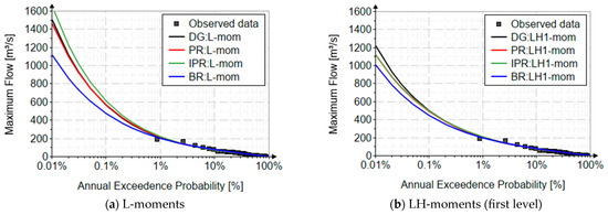
Figure 2. The graphical results for the Jijia River—Dorohoi Station.

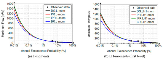
Figure 3. The graphical results for the Buhai River—Padureni Station.

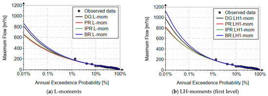
Figure 4. The graphical results for the Miletin River—Sipote Station.

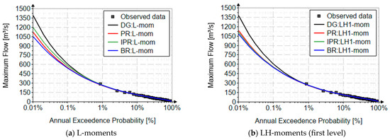
Figure 5. The graphical results for the Sitna River—Todireni Station.

In order to emphasize the heavy tail (the domain of rare events), the decimal logarithmic scale was employed on the horizontal axis.

As can be seen from the results, the values generated in the field of annual excess probabilities less than 1%, have a variability depending on the particularities of each analyzed distribution, the influence being given by the number of parameters that characterize each distribution. The DG, PR and IPR distributions have three parameters, properly calibrating the L-skewness, but generating different values of the L-kurtosis, an extremely important aspect in choosing the best distribution using these estimation methods. The four-parameter Burr distribution properly calibrates all four linear moments specific to the two analyzed methods.

Examining the results for the probability of exceeding 0.01%, it can be observed that, for Jijia River, they vary between 1652 m³/s (IPR distribution) and 1116 m³/s (BR4 distribution) using L-moments, between 1219 m³/s (DG distribution) and 1005 m³/s (BR4 distribution) using LH-moments. In the case of the Buhai river, the maximum flows vary between 1505 m³/s (IPR distribution) and 1176 m³/s (BR4 distribution) using L-moments, between 1257 m³/s (DG distribution) and 968 m³/s (BR4 distribution) using LH-moments. For the Miletin river, these maximum values vary between 863 m³/s (BR4 distribution) and 649 m³/s (PR distribution) using L-moments, between 1122 m³/s (BR4 distribution) and 799 m³/s (IPR distribution) using LH-moments. The results in the case of the Sitna river vary between 1388 m³/s (DG distribution) and 1049 m³/s (BR4 distribution) using L-moments, between 1379 m³/s (DG distribution) and 1083 m³/s (BR4 distribution) using LH-moments.

The differences in the distribution curves and the resulting quantile values, for the two estimation methods, are mainly due to the variation of the parameter that characterizes L-skewness, which imposes a different behavior, especially in the area of rare and very rare events, with a more or less pronounced heavy tail. As could be observed in the case of other distributions from other families [5,11] using the L-moments method, this stability between methods of some distributions, is due to the reduced variability of the distribution parameter that characterizes L-skewness, LH-skewness, around the value of the sample L-skewness.

4.2. Best-Fit Distribution Selection

The main advantage of the analyzed methods, compared to other estimation methods (the method of ordinary moments, the method of maximum likelihood, the method of least squares, the principle of maximum entropy, etc.), is that there is a more rigorous selection criterion.

In general, due to the small lengths of the data series, statistical tests and performance metrics are only valid in the field of empirical probabilities (recorded data). Outside of this field, indicators and statistical tests lose their relevance (especially in the case of small and medium data series), because it is desired to determine the maximum values for small annual probabilities, where generally there is no recorded data.

Table 8 shows the performance quotes used in the case of the four case studies, with the mention that the RAE (the relative absolute error) and RME (the relative mean error) indicators [43,44,45] are relevant only in the conditions described previously:

$$\mathrm{R}\mathrm{M}\mathrm{E}=\frac{1}{\mathrm{n}}\cdot \sqrt{{{\displaystyle \sum _{\mathrm{i}=1}^{\mathrm{n}}\left(\frac{{\mathrm{x}}_{\mathrm{i}}-\mathrm{x}\left(\mathrm{p}\right)}{{\mathrm{x}}_{\mathrm{i}}}\right)}}^2}$$

(41)

$$\mathrm{R}\mathrm{A}\mathrm{E}=\frac{1}{\mathrm{n}}\cdot {\displaystyle \sum _{\mathrm{i}=1}^{\mathrm{n}}\left|\frac{{\mathrm{x}}_{\mathrm{i}}-\mathrm{x}\left(\mathrm{p}\right)}{{\mathrm{x}}_{\mathrm{i}}}\right|}$$

(42)

where $\mathrm{n},{\mathrm{x}}_{\mathrm{i}}$ and $\mathrm{x}\left(\mathrm{p}\right)$ represent the length of the recorded series, the observed value, and the estimated value for a given probability.

Table 8. Performance measurement for the Jijia, Buhai, Miletin and Sitna Rivers.

Distribution	L-Moments				Observed Data		LH-Moments				Observed Data
	RME	RAE	${\mathit{\tau }}_3$	${\mathit{\tau }}_4$	${\mathit{\tau }}_3$	${\mathit{\tau }}_4$	RME	RAE	${\mathit{\tau }}_{\mathit{H}3}$	${\mathit{\tau }}_{\mathit{H}4}$	${\mathit{\tau }}_{\mathit{H}3}$	${\mathit{\tau }}_{\mathit{H}4}$
	Jijia River
DG	0.0319	0.1724	0.4483	0.2881	0.4483	0.2436	0.0415	0.2125	0.4247	0.2586	0.4247	0.2307
PR	0.0773	0.2668		0.3106			0.1867	0.5742		0.2717
IPR	0.119	0.3504		0.3327			0.2714	0.7564		0.2777
BR4	0.0287	0.1476		0.2436			0.0651	0.2426		0.2307
	Buhai River
DG	0.0327	0.1252	0.5607	0.4157	0.5607	0.3731	0.0478	0.1986	0.5319	0.3689	0.5319	0.3303
PR	0.0341	0.1186		0.4115			0.0799	0.2493		0.3684
IPR	0.061	0.166		0.4309			0.14	0.3625		0.375
BR4	0.0305	0.1312		0.3731			0.0899	0.2695		0.3303
	Miletin River
DG	0.0292	0.1275	0.3041	0.2143	0.3041	0.2698	0.0399	0.1424	0.3912	0.2596	0.3912	0.3175
PR	0.0402	0.1544		0.2125			0.0552	0.1992		0.2457
IPR	0.0619	0.1858		0.2300			0.0473	0.1706		0.2507
BR4	0.0635	0.1852		0.2698			0.0603	0.2095		0.3175
	Sitna River
DG	0.0174	0.0781	0.3513	0.2470	0.3513	0.2451	0.0175	0.0781	0.3923	0.257	0.3923	0.2496
PR	0.0221	0.089		0.2406			0.0205	0.0872		0.2465
IPR	0.0399	0.1172		0.2606			0.0482	0.1276		0.2516
BR4	0.0341	0.1084		0.2451			0.0435	0.1202		0.2496

According to the results of the statistical indicators of the probability distributions, for the two analyzed methods (L- and LH-moments), the BR4 distribution has the best results, since it is a four-parameter distribution which calibrates accordingly all linear moments. The theoretical values of the statistical indicators of the distribution best approximate those of the data set.

Although the DG, PR and IPR distributions have a lower number of parameters than the BR4 distribution, it can be seen that these distributions have applicability in FFA, as long as the use of the distributions respects as much as possible the selection criteria imposed by the analyzed methods.

Thus, it can be observed that in certain situations the three-parameter distributions can represent alternatives to the four-parameter distributions whose applicability requires more laborious calculations. This aspect is all the more important since for many distributions there are approximate relationships for parameter estimation, characterized by very small errors, which greatly simplifies the calculation. The same can be observed in the case of the Siret and Buhai Rivers, where the PR distribution can be used as an alternative to the BR4 distribution, similarly with the DG distribution in the case of the Miletin River, the values generated for Q_0.01% being characterized by a bias of less than 20%, a more than acceptable error regarding the rarity of this event.

Considering that this represents the main preselection and selection criterion of the best fit distribution, the approximate relationships of the L-kurtosis–L-skewness variation are necessary. This information is presented in detail in Supplementary File.

4.3. Confidence Intervals

Taking into account the relatively short length of the analyzed series, the RME and RAE performance indicators are presented as indicative, making a performance classification valid only for the probability area of the recorded data, observation also valid for statistical tests such as Kolmogorov–Smirnov [46], Anderson-Darling, Akaike Information Criteria and Bayesian Information Criteria.

It is noteworthy that the quantile results exhibit some degree of uncertainty, mostly due to the short data length and the inability of three-parameter distributions to accurately calibrate the fourth-order linear moment.

The statistical uncertainties resulting from the variability of the observed data length, as demonstrated by other materials [47], need to be emphasized on three levels that are particular to the parameter estimation method: the estimation of statistical indicators, the estimation of parameters, and—most importantly—the estimation of quantiles.

The confidence interval (C.I) for these distributions must be shown, in light of all these statistical uncertainties. In this article, the interval is built based on Chow’s relation [48], presented and promoted by another research such as those in Bulletin 17B, Bulletin 17 C, Rao et al. [1,3,4,48], being a simplified approach, using the quantile and the frequency factor specific to the LH-moments, information also presented in previous materials [4,11,12,13]. Of course, there are other ways to calculate the C.I as well, including the conventional Bootstrap procedure [49,50,51], but these still have certain drawbacks, need a more involved analysis, and are not available to everyone.

Figure 6, Figure 7, Figure 8 and Figure 9 highlights the quantiles of the distributions with the analyzed estimation methods, as well as the confidence interval for the L- and LH-moments.

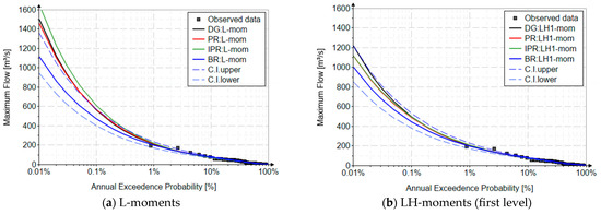
Figure 6. The confidence interval for the best fit model: Jijia River—Dorohoi Station.

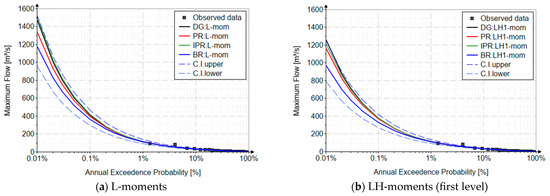
Figure 7. The confidence interval for the best fit model: Buhai River—Padureni Station.

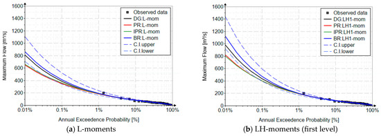
Figure 8. The confidence interval for the best fit model: Miletin River—Sipote Station.

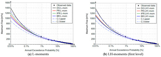
Figure 9. The confidence interval for the best fit model: Sitna River—Todireni Station.

It is recommended to include an easy method for the confidence interval, even based on a Gaussian assumption, if we consider that the existing Romanian legislation [52] for determining the maximum flows suffers from great deficiencies, both in terms of the use of distributions and parameter estimation methods, but especially of the recommendations regarding the determination of the confidence interval (the respective normative contains non-technical elements, such as the uncertainty interval [52,53]).

5. Conclusions

In the recent period, the use of these distributions from the generalized beta families has been greatly simplified with the presentation of important elements to apply in FFA, using MOM, and similarly in L-moments.

Considering the main advantage of the LH-moments, namely the fulfillment of the so-called “separation effect” of the maximum flow rates, this article presents all the exact and approximate relationships necessary for their use using this parameter estimation method.

The approximate relations for the frequency factors are a significant benefit in determining the maximum values of the flows for the required probability.

Another element of particular importance is the relationships and variation diagrams of the higher-order statistical indicators; they represent the main selection criterion of the best-fit distribution in the case of these parameter estimation methods. It also constitutes the basis for the preselection of certain distributions in FFA, especially regarding three-parameter distributions, using the two methods.

The performances of the analyzed distributions are checked on the four case studies, i.e., the Jijia, Buhai, Miletin and Sitna Rivers, from Romania, to find the maximum flows corresponding to the interested probabilities.

Following the results obtained, the BR4 distribution gives the best results for all four case studies, with the values of their theoretical statistical indicators correspondingly calibrating the similar values of the analyzed series. Among the distributions with three parameters, the best results were obtained by the distribution DG (Jijia and Sitna), followed by the distributions PR (Buhai) and IPR (Miletin). However, it should be highlighted that the results do not differ much from the BR4 distribution, the values being in general (for the maximum flow with the annual probability of exceeding 0.01%) below 20%, which represent a more than acceptable error considering this very rare event. The advantage of using PR and IPR distributions is that the parameters are considerably easier to estimate due to the availability of approximate relations for their estimation, thus avoiding solving systems of nonlinear equations, which are frequently an impediment.

The novelty elements presented regarding these methods will help researchers in frequency analysis, thus offering, in addition to classical approaches, other means of analyzing extreme events in hydrology.

The article does not rule out the use of different parameter estimation methods and probability distributions, especially as their relevant information has already been covered in prior papers, both in terms of the presentation of inverse functions, exact and approximate estimation relations of the parameters for different methods, diagrams and relationships of variation of high-order indicators characteristic of the methods, graphs of variation of shape parameters for different methods (and their comparative presentation),

The research presented in this article supplements the broader research begun within the Faculty of Hydrotechnics on the proposal to develop some norms regarding frequency analysis in hydrology for maximum flows, average flows, low flows, and hydrological drought, the results of which have been presented in previous materials [5,9,10,11,12,13,31].

All of these new aspects will be provided in separate open-source applications, making it easier to apply these probability distributions and parameter estimate methods in extreme event frequency investigations.

References

- Rao, A.R.; Hamed, K.H. Flood Frequency Analysis; CRC Press LLC: Boca Raton, FL, USA, 2000. [Google Scholar]
- Gaume, E. Flood frequency analysis: The Bayesian choice. WIREs Water 2018, 5, e1290. [Google Scholar] [CrossRef]
- Bulletin 17B Guidelines for Determining Flood Flow Frequency; Hydrology Subcommittee; Interagency Advisory Committee on Water Data; U.S. Department of the Interior; U.S. Geological Survey; Office of Water Data Coordination: Reston, VA, USA, 1981.
- Bulletin 17C Guidelines for Determining Flood Flow Frequency; U.S. Department of the Interior, U.S. Geological Survey: Reston, VA, USA, 2017.
- Anghel, C.G.; Ilinca, C. Evaluation of Various Generalized Pareto Probability Distributions for Flood Frequency Analysis. Water 2023, 15, 1557. [Google Scholar] [CrossRef]
- Hosking, J.R.M.; Wallis, J.R. Regional Frequency Analysis: An Approach Based on L-Moments; Cambridge University Press: Cambridge, UK, 1997. [Google Scholar] [CrossRef]
- Hosking, J.R.M. L-moments: Analysis and Estimation of Distributions using Linear, Combinations of Order Statistics. J. R. Statist. Soc. 1990, 52, 105–124. [Google Scholar] [CrossRef]
- Singh, V.P. Entropy-Based Parameter Estimation in Hydrology; Springer Science + Business Media: Dordrecht, The Netherlands, 1998. [Google Scholar]
- Ilinca, C.; Anghel, C.G. Flood-Frequency Analysis for Dams in Romania. Water 2022, 14, 2884. [Google Scholar] [CrossRef]
- Anghel, C.G.; Ilinca, C. Hydrological Drought Frequency Analysis in Water Management Using Univariate Distributions. Appl. Sci. 2023, 13, 3055. [Google Scholar] [CrossRef]
- Ilinca, C.; Anghel, C.G. Flood Frequency Analysis Using the Gamma Family Probability Distributions. Water 2023, 15, 1389. [Google Scholar] [CrossRef]
- Anghel, C.G.; Ilinca, C. Parameter Estimation for Some Probability Distributions Used in Hydrology. Appl. Sci. 2022, 12, 12588. [Google Scholar] [CrossRef]
- Ilinca, C.; Anghel, C.G. Frequency Analysis of Extreme Events Using the Univariate Beta Family Probability Distributions. Appl. Sci. 2023, 13, 4640. [Google Scholar] [CrossRef]
- Greenwood, J.A.; Landwehr, J.M.; Matalas, N.C.; Wallis, J.R. Probability Weighted Moments: Definition and Relation to Parameters of Several Distributions Expressable in Inverse Form. Water Resour. Res. 1979, 15, 1049–1054. [Google Scholar] [CrossRef]
- Murshed, S.; Park, B.-J.; Jeong, B.-Y.; Park, J.-S. LH-Moments of Some Distributions Useful in Hydrology. Commun. Stat. Appl. Methods 2009, 16, 647–658. [Google Scholar] [CrossRef]
- Papukdee, N.; Park, J.-S.; Busababodhin, P. Penalized likelihood approach for the four-parameter kappa distribution. J. Appl. Stat. 2022, 49, 1559–1573. [Google Scholar] [CrossRef] [PubMed]
- Shin, Y.; Park, J.-S. Modeling climate extremes using the four-parameter kappa distribution for r-largest order statistics. Weather Clim. Extremes 2023, 39, 100533. [Google Scholar] [CrossRef]
- Wang, Q.J. LH moments for statistical analysis of extreme events. Water Resour. Res. 1997, 33, 2841–2848. [Google Scholar] [CrossRef]
- Houghton, J.C. Birth of a parent: The Wakeby distribution for modeling flood flows. Water Resour. Res. 1978, 14, 1105–1109. [Google Scholar] [CrossRef]
- Meshgi, A.; Davar, K. Comprehensive evaluation of regional flood frequency analysis by L- and LH-moments. II. Development of LH-moments parameters for the generalized Pareto and generalized logistic distributions. Stoch. Environ. Res. Risk Assess. 2009, 23, 137–152. [Google Scholar] [CrossRef]
- Meshgi, A.; Khalili, D. Comprehensive evaluation of regional flood frequency analysis by L- and LH-moments. I. A revisit to regional homogeneity. Stoch. Environ. Res. Risk Assess. 2009, 23, 119–135. [Google Scholar] [CrossRef]
- Bhuyan, A.; Borah, M.; Kumar, R. Regional Flood Frequency Analysis of North-Bank of the River Brahmaputra by Using LH-Moments. Water Resour. Manag. 2010, 24, 1779–1790. [Google Scholar] [CrossRef]
- Gheidari, M.H.N. Comparisons of the L- and LH-moments in the selection of the best distribution for regional flood frequency analysis in Lake Urmia Basin. Civ. Eng. Environ. Syst. 2013, 30, 72–84. [Google Scholar] [CrossRef]
- Wang, Q.J. Approximate Goodness-of-Fit Tests of fitted generalized extreme value distributions using LH moments. Water Resour. Res. 1998, 34, 3497–3502. [Google Scholar] [CrossRef]
- Fawad, M.; Cassalho, F.; Ren, J.; Chen, L.; Yan, T. State-of-the-Art Statistical Approaches for Estimating Flood Events. Entropy 2022, 24, 898. [Google Scholar] [CrossRef]
- Lee, S.H.; Maeng, S.J. Comparison and analysis of design floods by the change in the order of LH-moment methods. Irrig. Drain. 2003, 52, 231–245. [Google Scholar] [CrossRef]
- Hewa, G.A.; Wang, Q.J.; McMahon, T.A.; Nathan, R.J.; Peel, M.C. Generalized extreme value distribution fitted by LH moments for low-flow frequency analysis. Water Resour. Res. 2007, 43, W06301. [Google Scholar] [CrossRef]
- Deka, S.; Borah, M.; Kakaty, S.C. Statistical analysis of annual maximum rainfall in North-East India: An application of LH-moments. Theor. Appl. Climatol. 2011, 104, 111–122. [Google Scholar] [CrossRef]
- Zakaria, Z.A.; Suleiman, J.M.A.; Mohamad, M. Rainfall frequency analysis using LH-moments approach: A case of Kemaman Station, Malaysia. Int. J. Eng. Technol. 2018, 7, 107–110. [Google Scholar] [CrossRef]
- Bora, D.J.; Borah, M. Regional analysis of maximum rainfall using L-moment and LH-moment: A comparative case study for the northeast India. J. Appl. Nat. Sci. 2017, 9, 2366–2371. [Google Scholar] [CrossRef]
- Anghel, C.G.; Ilinca, C. Predicting Flood Frequency with the LH-Moments Method: A Case Study of Prigor River, Romania. Water 2023, 15, 2077. [Google Scholar] [CrossRef]
- Crooks, G.E. Field Guide to Continuous Probability Distributions; Berkeley Institute for Theoretical Science: Berkeley, CA, USA, 2019. [Google Scholar]
- Domma, F.; Condino, F. Use of the Beta-Dagum and Beta-Singh-Maddala distributions for modeling hydrologic data. Stoch. Environ. Res. Risk Assess. 2017, 31, 799–813. [Google Scholar] [CrossRef]
- Ministry of the Environment. The Romanian Water Classification Atlas, Part I—Morpho-Hydrographic Data on the Surface Hydrographic Network; Ministry of the Environment: Bucharest, Romania, 1992. [Google Scholar]
- Kołodziejczyk, K.; Rutkowska, A. Estimation of the Peak over Threshold-Based Design Rainfall and Its Spatial Variability in the Upper Vistula River Basin, Poland. Water 2023, 15, 1316. [Google Scholar] [CrossRef]
- Kolaković, S.; Mandić, V.; Stojković, M.; Jeftenić, G.; Stipić, D.; Kolaković, S. Estimation of Large River Design Floods Using the Peaks-Over-Threshold (POT) Method. Sustainability 2023, 15, 5573. [Google Scholar] [CrossRef]
- Zhao, X.; Zhang, Z.; Cheng, W.; Zhang, P. A New Parameter Estimator for the Generalized Pareto Distribution under the Peaks over Threshold Framework. Mathematics 2019, 7, 406. [Google Scholar] [CrossRef]
- Gharib, A.; Davies, E.G.R.; Goss, G.G.; Faramarzi, M. Assessment of the Combined Effects of Threshold Selection and Parameter Estimation of Generalized Pareto Distribution with Applications to Flood Frequency Analysis. Water 2017, 9, 692. [Google Scholar] [CrossRef]
- Ciupak, M.; Ozga-Zielinski, B.; Tokarczyk, T.; Adamowski, J. A Probabilistic Model for Maximum Rainfall Frequency Analysis. Water 2021, 13, 2688. [Google Scholar] [CrossRef]
- Shao, Y.; Zhao, J.; Xu, J.; Fu, A.; Wu, J. Revision of Frequency Estimates of Extreme Precipitation Based on the Annual Maximum Series in the Jiangsu Province in China. Water 2021, 13, 1832. [Google Scholar] [CrossRef]
- Dau, Q.V.; Kangrang, A.; Kuntiyawichai, K. Probability-Based Rule Curves for Multi-Purpose Reservoir System in the Seine River Basin, France. Water 2023, 15, 1732. [Google Scholar] [CrossRef]
- Yah, A.S.; Nor, N.M.; Rohashikin, N.; Ramli, N.A.; Ahmad, F.; Ul-Sau, A.Z. Determination of the Probability Plotting Position for Type I Extreme Value Distribution. J. Appl. Sci. 2012, 12, 1501–1506. [Google Scholar] [CrossRef][Green Version]
- Singh, V.P.; Singh, K. Parameter Estimation for Log-Pearson Type III Distribution by POME. J. Hydraul. Eng. 1988, 114, 112–122. [Google Scholar] [CrossRef]
- Shaikh, M.P.; Yadav, S.M.; Manekar, V.L. Assessment of the empirical methods for the development of the synthetic unit hydrograph: A case study of a semi-arid river basin. Water Pract. Technol. 2021, 17, 139–156. [Google Scholar] [CrossRef]
- Gu, J.; Liu, S.; Zhou, Z.; Chalov, S.R.; Zhuang, Q. A Stacking Ensemble Learning Model for Monthly Rainfall Prediction in the Taihu Basin, China. Water 2022, 14, 492. [Google Scholar] [CrossRef]
- Miniussi, A.; Marani, M.; Villarini, G. Metastatistical Extreme Value Distribution applied to floods across the continental United States. Adv. Water Resour. 2020, 136, 103498. [Google Scholar] [CrossRef]
- Singh, V.P.; Guo, H. Parameter estimation for 2-Parameter log-logistic distribution (LLD2) by maximum entropy. Civ. Eng. Syst. 1995, 12, 343–357. [Google Scholar] [CrossRef]
- Chow, V.T.; Maidment, D.R.; Mays, L.W. Applied Hydrology; McGraw-Hill, Inc.: New York, NY, USA, 1988; ISBN 007-010810-2. [Google Scholar]
- Rao, G.S.; Albassam, M.; Aslam, M. Evaluation of Bootstrap Confidence Intervals Using a New Non-Normal Process Capability Index. Symmetry 2019, 11, 484. [Google Scholar] [CrossRef]
- Beaumont, J.-F.; Émond, N. A Bootstrap Variance Estimation Method for Multistage Sampling and Two-Phase Sampling When Poisson Sampling Is Used at the Second Phase. Stats 2022, 5, 339–357. [Google Scholar] [CrossRef]
- Bochniak, A.; Kluza, P.A.; Kuna-Broniowska, I.; Koszel, M. Application of Non-Parametric Bootstrap Confidence Intervals for Evaluation of the Expected Value of the Droplet Stain Diameter Following the Spraying Process. Sustainability 2019, 11, 7037. [Google Scholar] [CrossRef]
- Ministry of Regional Development and Tourism. The Regulations Regarding the Establishment of Maximum Flows and Volumes for the Calculation of Hydrotechnical Retention Constructions; Indicative NP 129–2011; Ministry of Regional Development and Tourism: Bucharest, Romania, 2012. [Google Scholar]
- Drobot, R.; Draghia, A.F.; Chendes, V.; Sirbu, N.; Dinu, C. Consideratii privind viiturile sintetice pe Dunare. Hidrotehnica 2023, 68, 37–52. (In Romanian) [Google Scholar]
Disclaimer/Publisher’s Note: The statements, opinions and data contained in all publications are solely those of the individual author(s) and contributor(s) and not of MDPI and/or the editor(s). MDPI and/or the editor(s) disclaim responsibility for any injury to people or property resulting from any ideas, methods, instructions or products referred to in the content. |
© 2023 by the authors. Licensee MDPI, Basel, Switzerland. This article is an open access article distributed under the terms and conditions of the Creative Commons Attribution (CC BY) license (https://creativecommons.org/licenses/by/4.0/).