


Abstract
Oblique and Fork-shaped traces in ionosonde’s ionograms have been identified as manifestations of nighttime and daytime Medium-Scale Traveling Ionospheric Disturbances (MSTIDs), respectively. The MSTIDs associated with these singular patterns have been verified by analyzing the evolution of detrended total electron content (dTEC) perturbation maps derived from the Global Navigation Satellite System (GNSS) signals. This has made it possible to create a database of MSTIDs characterized by their dominant period, horizontal propagation speed, wavelength, and propagation direction. This also allowed comprehensive case studies and statistical analyses of their temporal occurrence, direction of propagation, seasonal dependence, and its association with Spread-F (SF) phenomena. The results reveal that approximately 92% of the “Oblique” traces and 86% of the “Fork” traces in ionograms correspond to nighttime and daytime MSTID activity, respectively, as observed in the dTEC maps. Oblique traces are predominantly observed during southwestward propagating MSTIDs and exhibit a marked seasonal occurrence during summer and winter. Fork traces occurred predominantly during equatorward propagating MSTIDs and are most frequently observed in winter. A statistically significant association has been found between daytime MSTID activity (Fork traces) and the subsequent appearance of SF, with conditional probabilities ranging from ~87% to ~78% at mid-to-high latitudes and from ~76% to ~61% at mid-to-low latitudes. However, when overall MSTID activity was considered—taking into account both the disturbances associated with the daytime Forks and those associated with nighttime Oblique traces—the statistical association with subsequent occurrence of SF increased to approximately 91%. These results show a strong statistical relationship but do not establish a direct causal link between an individual daytime MSTID activity and nighttime SF. Instead, the occurrence of MSTID is seen as an indicator of ionospheric conditions that are favorable for the development of SF at mid-latitudes. These findings offer new insights into the ionogram-based characterization of MSTID signatures and their association with nighttime SF over Europe. The results highlight that MSTID occurrence serves as a strong indicator of favorable conditions for the development of instabilities in the mid-latitude ionosphere, offering valuable implications for the possible modeling of the ionosphere and the prediction of ionospheric weather.
1. Introduction
Since the early 1960s, extensive studies have been devoted to understanding travelling ionospheric disturbances (TIDs) and their fundamental role in ionospheric variability. Hines [1] first proposed that TIDs represent the ionospheric manifestation of atmospheric gravity waves (AGWs) that propagate upward from the lower atmosphere and perturb the ionospheric plasma at F-region heights. These gravity-wave-induced oscillations generate fluctuations in plasma density, leading to wave-like ionospheric structures detectable by a range of ionospheric sensors. Georges [2] summarized the early observational evidence of these disturbances, while Hunsucker [3] emphasized their central importance in coupling the neutral atmosphere and ionized plasma. Subsequent research established TIDs as a major component of ionospheric dynamics at mid-latitudes, with quasi-periodic plasma perturbations that can span from hundreds to thousands of kilometers [4]. These disturbances can significantly modulate the electron density distribution, affecting radio wave propagation, the accuracy of Global Navigational Satellite System (GNSS) positioning, and ionospheric stability [5,6].
TIDs are generally classified into two categories based on their spatial and temporal scales: large-scale TIDs (LSTIDs) and medium-scale TIDs (MSTIDs) [4]. LSTIDs are typically linked to geomagnetic activity and are driven by auroral processes, such as Joule heating and Lorentz forcing, in the high-latitude ionosphere. They have horizontal wavelengths exceeding 1500 km, phase velocities ranging from 400 to 1000 m/s, and periods of 30 to 180 min [3,7,8,9]. These large-scale disturbances generally propagate equatorward from the auroral zones and can traverse mid-latitudes during geomagnetically disturbed periods. The resulting perturbations manifest as travelling fronts of enhanced and depleted electron density, often accompanied by simultaneous thermospheric wind and temperature variations. The coupling mechanism involves the propagation of AGWs from the high-latitude energy deposition region, which then induces plasma motion through the action of meridional wind that redistributes ionization along geomagnetic field lines. In contrast, MSTIDs are more frequently observed during geomagnetically quiet conditions and are thought to originate primarily from lower-atmospheric sources or in situ electrodynamic instabilities [5]. They are characterized by horizontal wavelengths between 100 and 1500 km, horizontal phase velocities of approximately 50–400 m/s, and periods ranging from 15 min to about 1 h [3,4,10,11]. Unlike LSTIDs, which propagate nearly equatorward, MSTIDs at mid-latitudes typically travel southwestward (SW) at night and equatorward during the daytime in the Northern Hemisphere [5,11], in accordance with the background ionospheric wind and electric field. MSTIDs may manifest as periodic perturbations in F-region height, critical frequency (foF2), and total electron content (TEC). Their generation mechanisms include AGWs originating from tropospheric convection, orographic forcing, and jet stream activity that can propagate into the ionosphere, while internal electrodynamic processes can amplify these perturbations.
The development of MSTIDs involves a combination of neutral atmospheric forcing and ionospheric electrodynamics. AGW-induced perturbations can redistribute plasma through ion-neutral coupling, producing wave-like structures in electron density and F-region height. Observations have shown that nighttime MSTIDs frequently exhibit significant internal plasma drifts and electric-field perturbations, indicating that electrodynamic processes play an important role in their evolution [12,13]. In addition, Ogawa et al. [14] reported a daytime MSTID exhibiting LSTID-like propagation characteristics but lacking associated F-region irregularities, suggesting that the ionospheric response to travelling disturbances depends strongly on the prevailing background conditions.
One of the main electrodynamic processes invoked for the structuring of the nighttime F region in mid-latitude is the Perkins instability [15]. Its growth depends on the background electric field, the strength of the neutral wind, the geometry of the geomagnetic field, and the Pedersen conductivity of the F region integrated along the field lines. The isolated Perkins mode grows slowly, but the nighttime ionosphere does not behave as an isolated F region. Conductivity inhomogeneities within sporadic-E (Es) layers can support polarization electric fields, and since these fields efficiently transmit along geomagnetic field lines, perturbations in the E and F regions can become electrodynamically coupled [16,17]. Therefore, the coupled E–F instability can amplify and organize disturbances at F-region height more effectively than the isolated Perkins mode, while neutral wind perturbations driven by gravity waves (GWs) can provide an additional source of seeding and plasma redistribution [18,19,20]. These processes influence the magnitude and orientation of the ionospheric plasma disturbance, causing electron density gradients and tilted reflecting surfaces that affect the paths of radio signals probing the ionosphere.
Digital ionosondes, including Digisondes, have historically played a central role in detecting and interpreting TIDs. Since the mid-20th century, several distinctive ionogram features have been associated with travelling disturbances [21,22,23,24,25]. TIDs disturb both the distribution of electron density and the height of the F layer, producing horizontal density gradients and tilted or curved iso-density surfaces. The ionosonde transmissions reflected by the ionosphere can then return along more than one ray path, including an almost vertical return from the main layer and non-vertical returns from horizontally displaced or tilted parts of the disturbed layer. The coexistence and temporal evolution of these ray paths can produce cusp-like, loop-like, or bifurcated traces, as demonstrated by ray-tracing studies [21,22,26]. Oblique traces can be interpreted within the same geometrical framework when a sufficiently tilted or horizontally displaced reflecting region produces a secondary off-vertical return separated from the main F-layer trace [25,26]. “Fork” or “Cusp” structures in ionograms, which appear as Y- or U-shaped deformations near the upper end of the F-region echoes or bifurcations of the F-region trace are ionogram signatures of a horizontally non-uniform ionosphere. Thus, the immediate cause of the different ionogram morphologies is the geometry and strength of the TID-induced electron-density gradients and reflecting-surface tilts. Neutral winds, background electric fields, ionospheric conductivity, and E–F region coupling are upstream processes that control the formation and evolution of the disturbed plasma structure. The preferential nighttime occurrence of Oblique traces and daytime occurrence of Fork traces are therefore treated in this study as an observational result of induced ionospheric disturbances.
Spread-F (SF) [24,27,28] is an ionogram manifestation of a structured F region, but its physical interpretation depends strongly on latitude. At equatorial latitudes, post-sunset SF is commonly associated with plasma depletion structures generated through the generalized Rayleigh–Taylor instability [29]. Mid-latitude SF is physically distinct and should not automatically be interpreted as the same plasma-bubble process. At mid-latitudes, range and frequency SF can occur when the bottom-side F region develops pronounced horizontal or vertical electron-density gradients, tilted iso-density surfaces, and small-scale irregularities that provide multiple off-vertical, specular, or scattered return paths to the ionosonde [24,27,28,29,30,31,32]. MSTIDs can contribute to this environment by modulating the F-region height and electron-density gradients, while Perkins-instability growth, gravity-wave forcing, background electric fields and neutral winds, and E–F region electrodynamic coupling can amplify or organize the disturbed plasma [12,16,17,18,19,20]. Midlatitude SF should therefore be regarded as an observational signature of F-region plasma structuring rather than as a unique diagnostic of a single instability mechanism. Mid-latitude SF and its characteristic ionogram morphology are well documented in European Digisonde observations [27,28,33]; a representative manually confirmed SF ionogram is shown in Figure 1b of Paul et al. [33]. Previous investigations have reported a close relationship between TID/MSTID activity and midlatitude SF occurrence [24,27,34], motivating the present assessment of their statistical correspondence over the European sector.
Figure 1.
Example of ionograms showing Fork (or cusp) traces (a) and Obliquely reflected traces (b). The color bar indicates the vertical echoes and the horizontal arrival direction of the received for non-vertical echoes.
Despite extensive investigations of MSTIDs and their relationship with ionospheric irregularities, several aspects remain insufficiently understood. Most previous studies have identified MSTIDs using GNSS-derived TEC observations, airglow imaging, or radar measurements [11,15,35,36], while Digisonde observations have primarily been used to examine localized ionospheric responses and characteristic ionogram signatures associated with travelling disturbances [21,23,26].
The present study combines Digisonde observations from two European mid-latitude stations, Roquetes (Spain) and Dourbes (Belgium), with GNSS-derived detrended total electron content (dTEC) measurements to investigate MSTID activity during 2020 and 2024. The objectives of this research are (a) to identify and validate Fork and Oblique Digisonde signatures associated with MSTIDs using independent dTEC observations; (b) to characterize the associated MSTID properties in terms of dominant period, horizontal propagation velocity, wavelength, and propagation direction; and (c) to assess their statistical association with subsequent nighttime SF occurrence. Through this approach, the study provides a comprehensive assessment of Digisonde-observed MSTID signatures and their relationship with mid-latitude ionospheric irregularities. Section 2 describes the datasets and methodology; Section 3 and Section 4 present the results and discussion; and Section 5 summarizes the main findings.
2. Data and Methodology
To investigate TIDs and their possible association with nighttime SF over the mid-latitude region, we analyzed observations from two European Digisonde stations: Dourbes (geographic coordinates: 50.1° N, 4.6° E; geomagnetic latitude: 47.2° N; URSI Code: DB049) in Belgium and Roquetes (EBRE) (geographic coordinates: 40.8° N, 0.5° E; geomagnetic latitude: 36.1° N; URSI Code: EB040) in Spain. These stations were selected because they form a nearly north–south pair separated by about 10° in latitude, providing an ideal geometry for tracking meridional TID propagation across the mid-latitude ionosphere. Both sites maintain long-term, continuous Digisonde records and are supported by dense surrounding GNSS receiver networks, facilitating a combined ionogram–TEC analysis.
For this study, Digisonde and detrended Total Electron Content (dTEC) data were analyzed for two distinct solar activity years, 2020 and 2024. 2020 is a low solar activity year with an annual mean sunspot number (SSN) of 8.8 and an annual mean Kp index of 1.17, while 2024 represented a high solar activity year with an average SSN of 154.7 and an average Kp index of 1.92. Yearly solar indices were obtained from the Solar Influences Data Analysis Centre (SIDC) of the Royal Observatory of Belgium (https://www.sidc.be/SILSO/datafiles/; accessed on 8 May 2026), and the geomagnetic activity Kp index was obtained from the GFZ Helmholtz Centre for Geosciences website (https://kp.gfz.de/en/; accessed 21 August 2026).
2.1. Digisonde Observations
Both Dourbes and Roquetes operate modern DPS-4D digital Digisondes, which provide high-resolution ionograms suitable for detecting small-scale plasma irregularities. Ionogram data from these stations were obtained from the Digital Ionogram Database (DIDBase) (https://giro.uml.edu/ionoweb/; accessed on 10 April 2026) [37]. The nominal temporal cadence of ionogram recordings is 5 min. However, the available sampling was not uniform across the four station-year datasets. We quantified the availability of each station-year dataset based on the total number of recorded ionograms relative to the total number of ionograms that should have been recorded at a 5 min interval; that is, 105,408 expected over a full leap year (366 days × 288 5 min time intervals per day). Table 1 summarizes the annual and seasonal availability of the data sets, as well as the range of minimum to maximum availability across the 24 UT-hour sectors (UT-h range). Seasonal availability is indicated as percentages for December to February (DJF), for March to May (MAM), for June to August (JJA), and for September to November (SON).
Table 1.
Availability of Digisonde ionograms used in the 2020 and 2024 analyses at Dourbes and Roquetes after removing those where the phenomena could not be identified. See text for details.
The varying levels of data availability shown in Table 1 are the result of various technical issues that occurred with the recording sensors. These sampling differences were considered when interpreting the raw seasonal and diurnal distributions of the identified ionogram signatures.
All ionograms were visually inspected to identify signatures of TID activity and nighttime SF. Nighttime SF events were assessed during local post-sunset hours, spanning 16:00 UT to 08:00 UT of the following day [24], to capture the development of F-region irregularities. In contrast, the detection of TID activity was done for both daytime and nighttime ionograms.
Two distinctive ionogram signatures were used to identify TID activity:
- Fork (or cusp) traces, which appear as bifurcations of the main F-layer trace and are widely accepted indicators of TID passage [21,22]. Some examples are shown in Figure 1a.
- Obliquely reflected traces, which are less frequently documented but may arise from wavefront tilts associated with TID propagation [25]. Some examples are shown in Figure 1b.
Both signatures were systematically examined across all ionograms for Dourbes and Roquetes. The DPS-4D ionograms use color coding to indicate the horizontal arrival direction of the received echoes. Six directional classes are provided for non-vertical echoes: NNE (0° ≤ θ < 60°), E (60° ≤ θ < 120°), SSE (120° ≤ θ < 180°), SSW (180° ≤ θ < 240°), W (240° ≤ θ < 300°), and NNW (300° ≤ θ < 360°). Therefore, oblique-trace events contain directional information on the sector from which echoes arrive, and the temporal evolution of the color-coded secondary echoes across consecutive ionograms can be used to estimate the direction of propagation of the associated irregularities. However, Fork traces usually do not contain a distinct directional secondary echo from which the propagation direction of the associated irregularities could be inferred.
We conducted a visual inspection of the ionograms to classify nighttime SF events using the method for identifying SF in mid-latitudes described by Paul et al. [33]; we used this classification for further statistical analysis of the potential association of ionospheric irregularities with the SF. Two principal SF morphologies were distinguished during the inspection: Range SF (RSF), identified from vertical spreading of the F-region trace along the virtual-height axis (typically over approximately 10–50 km), and Frequency SF (FSF), identified from horizontal spreading of the F-region trace in frequency (typically over approximately 0.2–1 MHz). Ionograms exhibiting either morphology, including cases in which both forms of spreading were present, were treated as SF-positive for the binary occurrence analysis. RSF and FSF were thus distinguished during identification but were not analyzed as separate statistical populations in the present study. To avoid ambiguous classification, an SF event was considered valid only if it persisted through at least three consecutive ionograms (a minimum duration of 15 min, given the 5 min cadence) [24]. Ionograms in which the Es-layer blanketed or obscured the F-region trace or in which the F-region morphology could not be classified unambiguously were excluded from the analysis.
In addition to the ionogram observations, Digisonde skymap measurements were used to provide information on the ionospheric tilt angles associated with the detected disturbances. The corresponding phase data (.DFT files), available at the same 5 min temporal resolution as the ionograms, were obtained from the DriftBase repository (https://lgdc.uml.edu/common/DFDBFastStationList; accessed on 9 May 2026) and processed using Drift Explorer version 1.2.14 (https://giro.uml.edu/drift-explorer.html; accessed on 9 May 2026) following the methodology described by Paznukhov et al. [38]. At each 5 min epoch, the zenith angle of the received echo, obtained as 90° minus the measured elevation angle, was resolved into east–west and north–south tilt components using the corresponding echo’s azimuth. To emphasize short-term fluctuations in the orientation of the reflecting ionospheric surface, consecutive first differences and, subsequently, second differences of these components were calculated. The resulting quantities are referred to here as the E–W and N–S tilt deviations. No additional temporal smoothing or filtering was applied after this differencing procedure. The tilt deviations were used as a local consistency check for changes in the reflecting-surface geometry during the identified disturbed intervals.
2.2. GNSS dTEC Data
We use the global detrended total electron content (dTEC) data of the GRID2 product distributed and maintained by Nagoya University (https://stdb2.isee.nagoya-u.ac.jp/GPS/shinbori/GRID2/nc/; accessed on 14 May 2026) to examine whether Fork and Oblique signatures identified in the Digisonde ionograms were accompanied by TIDs and to characterize the corresponding TID-related TEC perturbations. The GRID2 files provide geographic latitude, geographic longitude, observation time, and dTEC values derived from the global GNSS receiver network. The dTEC field is distributed on a 0.25° × 0.25° geographic latitude–longitude sampling grid. The source product applies a 5 × 5 grid-cell spatial boxcar average, so the 0.25° grid spacing represents the sampling interval rather than an independent physical resolution at every grid point. The source-level averaging spans approximately five grid cells in each horizontal coordinate direction and therefore smooths structures approaching the smallest scales represented by the gridded product.
The dTEC represents short-period TEC perturbations relative to the slowly varying ionospheric background. The TEC-mapping and instrumental-bias framework follows Otsuka et al. [39], while the TID-scale perturbation component is obtained by removing a 1-h running average (±30 min) from the raw TEC time series as applied in the European MSTID analysis of Otsuka et al. [11]. No additional interpolation to a 0.15° × 0.15° grid and no additional 5° × 5° geographic smoothing were applied to the GRID2 data used in this analysis. The latitude, longitude, time, and dTEC variables were read directly from the NetCDF files and retained on the coordinates supplied by the archive. The 0.15° × 0.15° grid used in earlier regional European TEC-mapping studies was therefore not imposed on the GRID2 product analyzed here.
We extracted a station-centered subset of dTEC values with the same start and end times defined from the Digisonde ionogram sequence for each manually identified Fork or Oblique event. The spatial limits extended ±2.5° in geographic latitude and ±2.5° in geographic longitude from the corresponding Digisonde, yielding a 5° × 5° geographic analysis domain centered on Dourbes or Roquetes. This 5° × 5° region defines only the spatial search domain used to examine the TID-related TEC perturbation and is distinct from the source-level grid-cell averaging. Only dTEC records falling within the ionogram-defined event interval were retained; no additional temporal lag was introduced before or after the event. We organized the retained dTEC records into nominal 5 min. map epochs by rounding the archive timestamps to the nearest 5 min. and averaging records that shared the same epoch and geographic grid point for direct comparison with the 5 min. Digisonde observations. We generated in this way the sequential dTEC maps to be used for event validation without changing the geographic grid. The filtered GRID2 records at their archive timestamps were retained separately for the numerical TID-parameter calculations described below. Consequently, the map-based validation and the parameter-estimation stage used the same event subset without introducing additional spatial interpolation.
The source-level spatial averaging must be considered when interpreting the disturbance morphology and the derived propagation characteristics. Spatial averaging can reduce the apparent amplitude of localized TEC perturbations and smooth sharp horizontal TEC gradients, particularly for structures approaching the smallest scales represented by GRID2. The analysis therefore characterizes coherent regional-scale TID signatures resolved in the gridded dTEC field rather than the fine-scale plasma structure below the effective spatial resolution of the product.
2.2.1. Validation of Digisonde TID Signatures Using GNSS dTEC Observations
We applied the following criteria to validate whether ionogram signatures relate to TID activity. Each identified Fork and Oblique event was examined using the chronological sequence of dTEC maps covering the same ionogram-defined interval. The Digisonde–dTEC correspondence was constrained both spatially and temporally. Spatially, the associated dTEC perturbation was required to occur within the ±2.5° latitude–longitude region centered on the corresponding Digisonde. Temporally, the perturbation had to be present and exhibit coherent evolution during the same event interval identified from the ionograms. Thus, the ionogram and dTEC signatures were compared over their common event duration rather than through an independently imposed time-offset window. We additionally imposed a quantitative amplitude criterion to the spatial and temporal coherence of the dTEC disturbance: the magnitude of the dTEC perturbation was required to exceed 0.2 TECU within the station-centered region of analysis. Moreover, amplitude disturbance alone was not considered sufficient for TID identification. The perturbation was additionally required to exhibit an organized wave-like structure, with at least two coherent dTEC phase fronts and systematic horizontal progression through successive map epochs. Positive TEC perturbation crests and negative perturbation troughs were followed chronologically across the map sequence. Isolated dTEC enhancements or depletions that exceeded 0.2 TECU but did not maintain a coherent wavefront morphology or systematic phase progression were not accepted as evidence of a propagating TID. Therefore, 0.2 TECU dTEC disturbance, together with wavefront coherence, temporal evolution and matching the region of the Digisonde sensor, was used to validate whether ionogram signatures relate to TID activity.
Figure 2 illustrates the observational geometry used for this correspondence analysis. Consecutive dTEC maps show the displacement of a coherent perturbation pattern through time, while the propagation direction is assumed to be approximately normal to the orientation of the phase fronts. The schematic time-distance representation in Figure 1 is included to illustrate the physical meaning of systematic phase progression. Section 2.2.2 describes the numerical calculation of TID characteristics.
Figure 2.
Schematic representation of the procedure used to validate Digisonde-observed TID signatures and determine the propagation characteristics of the corresponding disturbances from GNSS-derived dTEC observations. (a) Schematic consecutive dTEC maps at t0, t1 = t0 + Δt, and t2 = t0 + 2Δt, showing the displacement of a selected same-phase wavefront, WFti (indicated by dotted lines), near the Digisonde location indicated by the black triangle. (b) Geometric representation of the tracked wavefront positions where arrows indicate the direction pointing to the geographic North and the direction of propagation of the wave front. The displacements ΔS1 and ΔS2 are measured in the direction normal to the wavefronts and are used to estimate the horizontal phase velocity, Vh. (c) Schematic time–distance representation of the dTEC perturbation along a transect oriented normal to the wavefronts, together with the corresponding local dTEC time series. The inclined perturbation bands indicate phase progression, while τ denotes the time interval between successive same-phase extrema.
The temporal evolution of the color-coded echoes of Oblique-trace events in the ionograms can provide information on the propagation sector of the disturbance, and this direction was compared with that obtained with the regional dTEC evolution. Therefore, Oblique events were retained in the directional statistics only when the ionogram-derived direction and the progression of the corresponding dTEC disturbance were consistent. Fork-trace events do not provide an equivalent directional estimation, and in these cases the propagation direction of the disturbance was obtained directly from the associated dTEC wavefront evolution.
2.2.2. Determination of MSTID Propagation Characteristics
If Fork- or Oblique-associated dTEC disturbance satisfied the spatial, temporal, amplitude, and coherence criteria described above, we calculated its respective dominant period, horizontal wavelength estimate, horizontal propagation speed, and propagation direction according to the following formulations.
Dominant Period
The dominant oscillation period, τ, was determined from the dTEC time series at the GRID2 point nearest to the geographic coordinates of the corresponding Digisonde station. Let x(tk) denote the dTEC value at epoch tk. The temporal mean over the event interval was first removed, and a Fast Fourier Transform was applied using the sampling interval of the retained GRID2 records. The zero-frequency component was excluded, and the positive-frequency component with the largest Fourier amplitude was identified as fpeak. The dominant period was then calculated as
where τ is expressed in minutes. When a valid positive-frequency spectral peak could not be determined, the duration between the first and last available dTEC records was used as the event’s temporal scale.
Horizontal Wavelength Estimation
The horizontal wavelength, λh, of the TID-associated dTEC perturbation was estimated from the spatial extent of the prominent peak-to-peak TEC response within the station-centered analysis region. The temporal peak-to-peak dTEC variation was evaluated at each geographic grid point, and the dominant spatially coherent perturbation region in the vicinity of the Digisonde was isolated from weaker peripheral variations. The geographic positions delimiting the latitudinal extent of this prominent perturbation region were identified, and their geodesic separation provided the basis for the estimate of λh.
This procedure characterizes the horizontal extent of the dominant coherent TID-related TEC perturbation resolved by GRID2. Because λh was obtained from the spatial extent of the prominent perturbation region rather than by directly measuring the separation between two adjacent same-phase crests in an individual dTEC map, it is interpreted as an operational estimate of the horizontal TID wavelength. The resulting value was therefore used consistently as an estimated horizontal wavelength in the subsequent propagation-parameter analysis.
Horizontal Propagation-Speed Estimation
For disturbances with dominant periods τ ≤ 60 min, the primary propagation-speed estimator followed the geographic position of the maximum positive dTEC perturbation through the available event records. If Pk denotes the latitude–longitude position of this positive dTEC maximum at time tk, the geodesic distances between consecutive positions were accumulated and divided by the elapsed time between the first and last valid records:
where dgeo(Pk, Pk+1) is the surface geodesic distance between successive positive-dTEC maxima in kilometers, tn − t1 is the total elapsed tracking time in seconds, and the factor 1000 converts kilometers to meters. Vtrack therefore represents the mean apparent horizontal propagation speed of the trajectory defined by the epoch-wise positive dTEC maximum. Because this estimator follows the positive dTEC maximum rather than tracking a single same-phase crest throughout the complete event, the resulting value is treated as an operational propagation-speed estimate rather than an exact phase velocity of an individually resolved TID wavefront.
For this short-period branch, propagation-speed estimates were constrained to a maximum of 600 m/s. When the tracking estimate exceeded this bound, or when a valid tracking estimate could not be obtained, an alternative speed was calculated by combining the operational horizontal wavelength estimate with the dominant period:
where λh is expressed in kilometers and τ in minutes. The factors 1000 and 60 convert distance and time to meters and seconds, respectively, yielding Vscale in m/s. When Vtrack exceeded 600 m/s, Vscale replaced it if Vscale ≤ 600 m/s; otherwise, the short-period estimate was limited to 600 m/s. The 600 m/s value was used only as an upper numerical safeguard in the propagation-speed calculation and was not used independently as a physical criterion for MSTID identification.
For disturbances with τ > 60 min, a separate local planar-gradient estimator was applied to represent the regional dTEC perturbation field. At each epoch, the fit used dTEC values within ±0.4° in geographic latitude and longitude of the Digisonde. At each epoch t, the local dTEC distribution was represented by
where φ and θ denote geographic latitude and longitude, respectively, and at, bt, and ct are the fitted planar coefficients at epoch t. The magnitude of the horizontal dTEC gradient was then calculated as
The gradient magnitude was converted to the empirical horizontal scale used by this estimator according to
where 111 km per geographic degree is the degree-to-distance conversion used in the calculation. Because gt is derived directly from the spatial gradient of the dTEC field, Lg is treated as an empirical gradient-derived spatial-scale proxy rather than a direct crest-to-crest TID wavelength. An epoch-wise propagation-speed estimate was subsequently obtained from Lg(t) and the dominant period, and the representative event value was defined as the median over the valid epochs:
where Lg is expressed in kilometers and τ in minutes, giving Vplane in m/s. For this long-period branch, an upper numerical bound of 2000 m/s was applied. When the plane-fit estimate was unavailable or zero, Vscale from Equation (3) was used as the alternative estimate, subject to the same 2000 m/s bound. As for the short-period branch, this 2000 m/s upper bound was applied only as a numerical safeguard to prevent unrealistically large values from poorly constrained estimates and was not used as a physical TID-classification threshold.
Propagation Direction and TID Scale Classification
The horizontal propagation direction was determined independently from the systematic spatial progression of coherent dTEC phase-fronts through successive map epochs. The propagation vector was taken approximately normal to the observed phase-front orientation and expressed as an azimuth α measured clockwise from the geographic north. For consistency with the directional classification of the Digisonde echo-direction classes, the dTEC-derived azimuths were grouped into six equal 60° sectors: NNE (0° ≤ α < 60°), E (60° ≤ α < 120°), SSE (120° ≤ α < 180°), SSW (180° ≤ α < 240°), W (240° ≤ α < 300°), and NNW (300° ≤ α < 360°).
For Oblique traces, the propagation sector inferred from the regional dTEC-derived phase-front progression was compared with the direction inferred independently from the color-coded secondary echoes in the ionograms. For Fork traces, which do not provide an equivalent directional secondary-echo signature, the propagation direction was obtained from the dTEC wavefront evolution and subsequently classified as poleward or equatorward according to the sign of its meridional component.
The validated disturbance population included structures spanning both medium- and large-scale TID regimes. The numerical velocity bounds described in the Horizontal Propagation-Speed Estimation Section were therefore treated only as computational safeguards and were not used as physical TID-classification thresholds. Identification of the MSTID subset was based on the combined temporal and spatial characteristics of the disturbance relative to the characteristic MSTID ranges discussed in Section 1, including periods of approximately 15–60 min, horizontal propagation speeds of approximately 50–400 m/s, and horizontal wavelengths generally below about 1500 km. These ranges are considered as characteristic rather than as discontinuous physical boundaries.
Because individual derived characteristics may extend beyond a conventional boundary owing to natural variability and characteristic-estimation uncertainty, an event was not reassigned to the large-scale category solely because one parameter crossed a nominal MSTID limit. Events exhibiting mixed or transitional characteristics were retained as an uncertain TID category. LSTIDs were identified when, at the event level, at least two of the three derived descriptors—dominant period, horizontal propagation speed, and horizontal wavelength—showed clear large-scale characteristics. This three-category treatment separates clearly large-scale disturbances from boundary or mixed cases while avoiding an artificial hard separation between the MSTID and LSTID populations. For the subsequent analyses explicitly based on MSTID occurrence or MSTID characteristics, only disturbances assigned to the MSTID category were included; uncertain TIDs and LSTIDs were excluded from those MSTID-specific calculations.
Uncertainty of the Derived TID Parameters
The horizontal wavelength estimate depends on two spatial limits delimiting the coherent perturbation region. Propagation of the localization uncertainty through these two endpoints gives representative one-standard-deviation wavelength uncertainties of approximately 30 km over Dourbes and 32 km over Roquetes, corresponding to Gaussian-equivalent 95% intervals of approximately ±59 km and ±62 km, respectively. These values quantify the uncertainty associated with localization of the perturbation limits; the source-level GRID2 smoothing remains an additional resolution limitation for structures approaching the smallest scales represented by the product.
The timing of each disturbance interval was defined by the 5 min Digisonde sequence. Treating the start and end boundaries as limited by the ionogram cadence gives a combined timing uncertainty of approximately 2 min at the one-standard-deviation equivalent level, or approximately ±4 min at the 95% equivalent level. The dominant period also depends on the finite duration of the dTEC series used in the FFT. Because the FFT frequency spacing is inversely proportional to the event duration, the period resolution is event-dependent and becomes progressively less precise for longer-period disturbances observed over comparatively short intervals. A single fixed Gaussian uncertainty was therefore not assigned to all FFT-derived periods.
The uncertainty of the horizontal propagation-speed estimate is likewise event-dependent because it depends on both the spatial localization and the elapsed tracking time. Propagation of the localization uncertainty through the available event-records gives a representative median one-standard-deviation velocity uncertainty of approximately 21 m/s, corresponding to a Gaussian-equivalent 95% interval of approximately ±42 m/s for a typical event; shorter-duration events exhibit larger uncertainty. Values equal to the numerical safeguards of 600 or 2000 m/s were treated as bounded computational estimates rather than independently resolved propagation speeds and were therefore not assigned symmetric Gaussian uncertainties.
Propagation direction was represented using six 60° azimuth sectors, giving a nominal directional resolution of approximately ±30°. The principal uncertainty and resolution contributions are summarized in Table 2. These estimates were used to interpret disturbances close to the conventional MSTID–LSTID transition, but they were not used to redefine the established occurrence percentages. Events showing mixed or boundary-scale parameter characteristics were retained as uncertain TIDs, whereas clearly large-scale disturbances were identified from the combined behavior of multiple derived characteristics, as described in the preceding section.
Table 2.
Principal uncertainty and resolution estimates associated with the GNSS dTEC-derived TID parameters. For the random localization and timing components, the quoted 95% values are Gaussian-equivalent intervals (approximately 1.96σ) provided as a common uncertainty scale. The GRID2 sampling interval and source-level smoothing footprint are reported separately as deterministic resolution limitations. The uncertainty of the FFT-derived period is event-dependent because it varies with the duration of the available dTEC interval.
3. Results
Following the methodology described in Section 2, daytime and nighttime TIDs identified from Digisonde Fork and Oblique trace signatures were validated using GNSS-derived dTEC observations. The validated disturbances were subsequently characterized in terms of their dominant period, wavelength, horizontal propagation speed, and propagation direction. The results of this analysis are presented in the following sections, beginning with representative examples of Oblique and Fork-trace events, followed by their statistical characteristics over the European mid-latitude sector.
3.1. Oblique Traces
Among the various TID signatures observed in ionograms, the Oblique trace represents one of the most distinctive yet comparatively understudied features. Although similar signatures have previously been reported [25,31,32], their physical interpretation and propagation characteristics have received limited attention. Earlier studies suggested that TID-related stratification in the F region may produce additional traces separated from the main ionogram trace. However, the relatively coarse temporal and spectral resolution available in earlier observations often made it difficult to distinguish these features from the main F-layer reflection or to determine their propagation characteristics. The availability of modern DPS-4D Digisonde observations, together with independent GNSS-derived dTEC measurements, provides an opportunity to investigate these signatures in greater detail.
3.1.1. Case: 25 February 2020
A representative example of an Oblique trace event observed over Roquetes on 25 February 2020 is presented in Figure 3a–h. Between 00:00 and 00:45 UT, a distinct secondary trace was observed in addition to the main F-layer reflection. The different colors shown in Figure 3a–g represent echoes arriving from different azimuthal directions. At 00:05 UT (Figure 3a), the Oblique trace appeared above the main F-layer trace and was detected in the northeastern sector. During the subsequent ionograms (Figure 3b,c), the separation between the Oblique and main traces progressively decreased until both traces nearly merged around 00:15 UT. Thereafter, the secondary trace reappeared and gradually moved away from the main trace toward the southwestern sector, remaining visible until approximately 00:45 UT (Figure 3d–g).
Figure 3.
Representative Oblique-trace event observed over Roquetes on 25 February 2020. Panels (a–g) show consecutive DPS-4D Digisonde ionograms between 00:05 and 00:40 UT, illustrating the temporal evolution of the Oblique trace relative to the main F-layer trace. Different colors indicate echoes arriving from different azimuthal directions. Panel (h) shows the temporal variation of the virtual heights of the main F-layer trace (black symbols) and the Oblique trace (red symbols). Blue arrows indicate the virtual-height separation between the two traces.
The temporal evolution of the event is summarized in Figure 3h, where the range of vertical echoes, the virtual height of the main trace, and the range of the Oblique traces are plotted as a function of time. The black symbols represent the virtual height of the F-layer trace, while the red symbols denote the range of the Oblique trace. The figure illustrates the progressive approach of the Oblique trace toward the main trace during the first half of the event, followed by its subsequent separation. The difference between the ranges of the vertical and oblique traces decreased from approximately 43.4 km at 00:05 UT to 15.4 km at 00:15 UT before increasing again to about 115 km by 00:40 UT. This systematic variation in virtual-height separation captures the complete evolution of the disturbance, indicating the passage of a travelling structure across the ionospheric reflection region. It should be noted that all heights shown in Figure 3h correspond to virtual heights derived from the ionograms (which in the case of oblique echoes should be interpreted as virtual slant ranges).
To examine rapid changes in the local orientation of the reflecting ionospheric surface, the E–W and N–S tilt deviations derived from the Roquetes Digisonde (EB040) were analyzed for the same interval. These quantities represent the second temporal differences of the corresponding tilt components rather than the absolute tilt angles. Figure 4a presents the values at 5 min resolution, with consecutive samples connected by straight line segments. The red dashed box marks the 00:00–00:45 UT interval during which the Oblique traces were observed. Marked alternating excursions are evident in both components during the early part of this interval, followed by lower-amplitude variability. Their coincidence with the Oblique-trace observations supports rapid changes in the local reflecting-surface geometry during the disturbance. The direction of propagation of the irregularity was inferred from the temporal evolution of the color-coded Oblique echoes and subsequently validated using the dTEC wavefront displacement.
Figure 4.
Validation of the Oblique-trace event shown in Figure 2. (a) North–south and east–west ionospheric tilt deviations derived at 5 min resolution from Roquetes (EB040) Digisonde observations on 25 February 2020. The red dashed box marks the 00:00–00:45 UT interval during which the Oblique traces were observed. (b) Consecutive GNSS-derived dTEC maps during the same interval. Roquetes (R) and Dourbes (D) are indicated by black triangles. White dashed lines mark the successive positions of a selected same-phase dTEC wavefront, while white arrows indicate the corresponding direction normal to the wavefront.
To independently verify the presence and propagation of the disturbance, GNSS-derived dTEC observations over Europe were examined. Figure 4b presents consecutive dTEC maps between 00:00 and 00:45 UT, with Roquetes (R) and Dourbes (D) Digisondes indicated by black triangles. The maps reveal coherent dTEC perturbation wavefronts oriented approximately NW–SE over the Roquetes region. The white dashed lines mark the successive positions of a selected same-phase wavefront, while the white arrows drawn perpendicular to the wavefront indicate its southwestward phase propagation. The systematic progression of the marked wavefront is consistent with the directional evolution inferred from the color-coded Oblique echoes in the ionograms (Figure 3).
The disturbance exhibited a maximum perturbation amplitude exceeding 0.4 TECU, a dominant period of approximately 45 min, a horizontal wavelength of about 422 km, and a horizontal propagation speed of approximately 380 m/sec. These characteristics are consistent with those commonly reported for MSTIDs in the literature [3,4,10,11]. The agreement between the directional evolution inferred from the ionograms and the independently derived dTEC wavefront progression, together with the supporting tilt-deviation variations, indicates that the observed Oblique traces were associated with an MSTID propagating across the Roquetes region from northeast toward southwest.
3.1.2. Statistical Presentation of Oblique Traces
To evaluate the occurrence characteristics of Oblique traces, all events identified over Roquetes and Dourbes during 2020 and 2024 were examined using the corresponding GNSS-derived dTEC observations. A total of 431 Oblique-trace cases were identified over Roquetes during the two study years, of which 19 did not show dTEC perturbations exceeding the adopted detection criterion. The remaining 412 cases were included in the characteristics analysis summarized in Table 3. On the other hand, 160 Oblique-trace cases were identified over Dourbes, with nine cases showing no corresponding dTEC perturbation. The remaining 151 cases were also included in the parameter analysis summarized in Table 3. The validated disturbances presented in Table 3 are separated into MSTIDs, uncertain TIDs, and LSTIDs according to the combined period, horizontal propagation-speed, and wavelength characteristics described in the Propagation Direction and TID Scale Classification Section.
Table 3.
Characteristics of TID events associated with Oblique traces over Dourbes and Roquetes during 2020 and 2024. “Uncertain” denotes events exhibiting mixed or transitional scale characteristics for which an unambiguous MSTID/LSTID assignment was not supported by the combined parameters. The listed ranges represent the observed values within each class rather than parameter-estimation uncertainties. The corresponding uncertainty estimates are summarized in Table 2.
The corresponding disturbance characteristics are presented separately for MSTIDs, uncertain TIDs, and LSTIDs in Table 3. A total of 328 out of 348 Oblique-associated TID cases over Roquetes were identified as MSTIDs in 2020, or approximately 94%. In addition, 58 out of 64 Oblique-associated TID cases were identified over Roquetes as MSTIDs in 2024, or approximately 91%. Approximately 95% of Oblique-associated TID cases, 54 out of 57, seen over Dourbes were identified as MSTIDs in 2020, and approximately 82%, or 77 out of 94 cases, in 2024. Overall, 517 of the 563 Oblique-associated disturbances included in the parameter analysis were classified as MSTIDs, corresponding to approximately 92% of the total. The remaining 46 cases comprised 18 uncertain TIDs and 28 LSTIDs. The uncertain population contains events with mixed or transitional temporal and spatial characteristics, whereas the LSTID population shows clear large-scale behavior in multiple derived characteristics. Separating these populations prevents the long-period and high-velocity extrema of the broader TID population from being interpreted as characteristic MSTID values. The Oblique-associated MSTID subset remained dominated by periods up to approximately 60 min and horizontal propagation speeds within approximately 400 m/s, while the substantially longer-period and higher-speed disturbances occurred within the uncertain and LSTID populations. The dominant propagation direction of the Oblique-associated MSTIDs remained southwestward.
Figure 5a–d illustrates the diurnal and annual distribution of Oblique-trace events over Roquetes and Dourbes during 2020 and 2024. The red and green curves denote sunset and sunrise, respectively, calculated at an ionospheric altitude of approximately 250 km, while the black markers identify Oblique traces temporally associated with nighttime SF. The colored markers denote the four populated Oblique-trace propagation sectors—SSW, SSE, NNE, and W—obtained by comparing the sector inferred from the temporal evolution of the color-coded ionogram echoes with the independently determined dTEC propagation sector.
Figure 5.
Annual and diurnal distribution of Oblique traces over (a) Roquetes in 2020, (b) Roquetes in 2024, (c) Dourbes in 2020, and (d) Dourbes in 2024.
Both the Digisonde and dTEC directions were classified using the same six 60° sectors. Four sectors were represented among the directionally validated events, while no validated cases occurred in the E or NNW sectors. Their absence from Figure 5 therefore reflects the observed directionally validated dataset rather than a mismatch between the two classification systems.
Oblique traces occurred predominantly between the sunset and sunrise curves, supporting their interpretation as primarily nighttime MSTID-related signatures. Over Roquetes in 2020, occurrences were observed during both summer and winter, whereas the 2024 events were concentrated mainly during summer. In winter, Oblique traces over Roquetes were detected broadly between 19:00 and 05:00 UT, while during summer they occurred between approximately 20:00 and 04:00 UT. At Dourbes, the corresponding occurrence intervals were approximately 18:00–06:00 UT in 2020 and 20:00–05:00 UT in 2024. Because Figure 5 presents individual events rather than normalized hourly occurrence rates, it should not be used to identify specific diurnal occurrence maxima.
The association between oblique traces and nighttime SF events was also quantified. Over Roquetes, the conditional association was approximately 65% in 2020 and increased to 75% in 2024. Over Dourbes, the association was 65% in 2020 but decreased to 58% in 2024. Overall, considering both stations and years, the oblique trace–SF association was approximately 66%. The observed latitudinal differences align with the findings of Otsuka et al. [11], who reported that the maximum occurrence rate of nighttime MSTIDs in Europe is around 50% at lower latitudes, while higher-latitude regions experience significantly fewer MSTID events.
To investigate whether the association between Oblique traces and nighttime SF varied with propagation direction, the events were grouped according to the four populated sectors of the common six-sector directional classification used in Figure 5. Figure 6 presents the total number of directionally validated Oblique traces and the corresponding events temporally associated with SF. Vertically hatched bars represent the total number of Oblique traces, while solid-colored bars represent the SF-associated subset.
Figure 6.
Propagation-direction distribution of directionally validated Oblique traces and their association with nighttime Spread-F over Roquetes and Dourbes during 2020 and 2024. Hatched bars indicate the total number of Oblique-trace events in the populated SSW, NNE, W, and SSE propagation sectors, while solid bars denote the corresponding events associated with nighttime Spread-F. The Digisonde- and dTEC-derived directions were classified using the same six 60° sectors, and an event was retained only when the two directional classifications were consistent. No directionally validated events occurred in the E or NNW sectors.
Among the four populated sectors, approximately 72% of the SF-associated directionally validated Oblique-trace events occurred in the SSW sector, while approximately 15% occurred in the SSE sector. Thus, disturbances propagating within the SSW sector represented the largest fraction of the SF-associated Oblique-trace population. These percentages refer to the complete SF-associated directionally validated population presented in Figure 6. Within the common six-sector classification, no directionally validated events occurred in the E or NNW sectors. The dominant southwestward propagation preference is consistent with previous observations of nighttime MSTIDs in the Northern Hemisphere [5,11].
3.2. Fork Traces
Fork traces represent one of the most widely recognized ionogram signatures of TIDs and have been reported extensively in previous ionosonde studies [21]. In the present study, Fork traces identified over Roquetes and Dourbes during 2020 and 2024 were independently validated using GNSS-derived dTEC observations and subsequently characterized in terms of the propagation properties.
3.2.1. Case: 3 August 2024
A representative Fork-trace event observed over Dourbes on 3 August 2024 is presented in Figure 7 and Figure 8a,b. Fork signatures were identified repeatedly between approximately 08:00 and 11:00 UT, forming one of the more prolonged daytime events in the dataset. Figure 6 shows selected ionograms during this interval, with the Fork structures highlighted by blue dashed circles. The signatures were not confined to a single isolated ionogram but appeared during several intervals, particularly around 08:30–08:50 UT, 09:10–09:35 UT, and 10:10–10:30 UT. The traces appear as bifurcated or cusp-like structures associated with the F-region reflection, indicating temporary deformation of the reflecting layer during the passage of the disturbances.
Figure 7.
Selected Digisonde ionograms from the representative Fork-trace event observed over Dourbes on 3 August 2024. The panels show observations at 08:10, 08:30, 09:10, 09:35, 10:25, and 10:50 UT. Blue dashed circles identify the recurrent bifurcated or cusp-like Fork signatures associated with the F-region reflection.
Figure 8.
Supporting observations for the Fork-trace event shown in Figure 7. (a) East–west and north–south ionospheric tilt deviations derived from Dourbes (DB049) Digisonde observations between 07:00 and 12:00 UT. The shaded region marks the approximately 08:00–11:00 UT interval during which recurrent Fork signatures were observed. The values are plotted at their original temporal resolution using straight line segments, without additional temporal smoothing or filtering. (b) Consecutive GNSS-derived dTEC maps between 08:00 and 10:45 UT. Dourbes (D) and Roquetes (R) are indicated by black triangles. White dashed lines mark representative coherent dTEC wavefronts in the individual snapshots, while white arrows indicate the corresponding direction perpendicular to the wavefronts.
To examine the corresponding local changes in the reflecting-surface geometry, the east–west and north–south tilt deviations derived from the Dourbes Digisonde (DB049) were analyzed between 07:00 and 12:00 UT. Figure 8a presents the tilt deviation time-series at the original temporal resolution, with consecutive values connected by straight line segments. No additional temporal smoothing or filtering was applied. The shaded interval denotes the approximately 08:00–11:00 UT period during which the recurrent Fork signatures were observed. The tilt deviations do not show a sustained enhancement throughout the complete shaded interval compared with the surrounding periods. However, intermittent excursions occur within the interval, including the most pronounced variation near 10:20 UT, which coincides with the clearer Fork signatures observed during approximately 10:10–10:30 UT. The tilt results are therefore considered supporting evidence of localized changes in the reflecting-surface geometry rather than independent confirmation of the complete event interval.
GNSS-derived dTEC observations were subsequently examined to independently verify the presence and propagation of associated ionospheric disturbances. Figure 8b presents consecutive dTEC maps between 08:00 and 10:45 UT, with Dourbes (D) and Roquetes (R) Digisondes indicated by black triangles. White dashed lines mark the positions of representative coherent dTEC wavefronts in the individual snapshots, while the white arrows are drawn perpendicular to the corresponding wavefronts and indicate their direction of phase propagation. Because several Fork episodes occurred during the analyzed interval, the marked structures represent successive coherent wavefronts observed during the event rather than one single wavefront tracked continuously throughout the complete three-hour period. Their temporal evolution shows predominantly equatorward propagation across the Dourbes region.
The dTEC analysis yielded a horizontal propagation speed of approximately 293 m/sec, a dominant period of about 60 min, and a horizontal wavelength of approximately 374 km. These values are consistent with MSTID activity. The recurrent Fork signatures and the independently observed dTEC wavefront progression therefore indicate that the event was associated with repeated equatorward-propagating MSTID activity over the European mid-latitude sector.
3.2.2. Statistical Presentation of Fork Traces
To characterize the disturbances associated with Fork traces, GNSS-derived dTEC perturbations were analyzed for all identified events over Roquetes and Dourbes during 2020 and 2024. A total of 526 Fork-trace cases were identified over Roquetes during the two years, of which 11 showed no corresponding dTEC according to the adopted detection criterion. The remaining 515 cases were included in the characteristics analysis summarized in Table 4. Similarly, 627 Fork-trace cases were identified over Dourbes, with 10 cases lacking a detectable dTEC signature; the remaining 617 cases were also included in Table 4. Again, the validated disturbances are separated into MSTIDs, uncertain TIDs, and LSTIDs according to the combined period, horizontal propagation-speed, and wavelength characteristics described in the Propagation Direction and TID Scale Classification Section.
Table 4.
Characteristics of TID events associated with Fork traces over Dourbes and Roquetes during 2020 and 2024. “Uncertain” denotes disturbances showing mixed or transitional scale characteristics that could not be assigned unambiguously to the MSTID or LSTID population. The listed ranges represent the observed parameter values within each class; numerical uncertainty estimates for the derived TID parameters are given separately in Table 2.
The corresponding disturbance characteristics are presented separately for MSTIDs, uncertain TIDs, and LSTIDs in Table 4. Approximately 83% of Fork-associated TIDs cases, 137 out of 165, were identified over Dourbes as MSTIDs in 2020, and approximately 88%, or 398 out of 452 cases, in 2024. Roquetes reports approximately 84% of Fork-trace-associated TIDs, or 354 out of 422 cases, as MSTIDs in 2020, and 90%, or 84 out of 93 events, in 2024. Overall, 973 of the 1132 Fork-associated disturbances included in the parameter analysis were classified as MSTIDs, corresponding to approximately 86% of the population. The remaining 159 disturbance events comprised 66 uncertain TIDs and 93 LSTIDs. The uncertain group contains events with mixed or transitional periods, propagation-speed, and wavelength characteristics, whereas the LSTID group shows clear large-scale behavior in multiple derived parameters. The Fork-associated MSTID subset exhibited periods predominantly within approximately 15–60 min and horizontal propagation speeds generally below approximately 400 m/s, whereas periods extending well beyond 1 h and the highest propagation-speed values occurred principally within the uncertain and LSTID populations. The dominant meridional propagation of the Fork-associated MSTIDs remained equatorward in all four station-year datasets.
Figure 9a–d presents the annual occurrence distribution of Fork traces over Roquetes and Dourbes during 2020 and 2024. The green and red curves denote the sunrise and sunset terminators, respectively, calculated at an altitude of approximately 250 km. The results show that Fork-trace occurrence is predominantly confined to daytime hours, generally between 08:00 and 16:00 UT. The only notable exception occurs at Dourbes during summer 2024, where several nighttime events were also observed. For both stations, Fork traces occur mainly after sunrise and persist throughout the daytime period, consistent with the known climatology of daytime MSTIDs.
Figure 9.
Annual and diurnal distribution of Fork traces over (a) Roquetes 2020, (b) Roquetes 2024, (c) Dourbes 2020, and (d) Dourbes 2024.
Seasonally, the highest occurrence is generally observed during winter months. Over Roquetes, the Fork-trace occurrence rate was higher in 2020 than in 2024, particularly during the latter half of the year, although the first half of 2024 was affected by data gaps. In contrast, Dourbes exhibited a marked increase in Fork-trace occurrence during 2024, together with a broader seasonal distribution. The difference between the two stations is relatively small during 2020 but becomes more pronounced in 2024, when Dourbes experienced a high number of daytime Fork-trace events. These observations are consistent with the climatological results of Otsuka et al. [11], who reported that daytime MSTID occurrence reaches a maximum during winter daytime hours and exhibits weaker latitudinal variability than nighttime MSTIDs. The predominance of daytime occurrence, together with the equatorward propagation identified from the dTEC observations, indicates that Fork traces provide a robust indicator of daytime MSTID activity over the European mid-latitude region.
3.2.3. Association Between Daytime Fork Trace and Nighttime SF
Daytime Fork-associated MSTIDs and nighttime SF can be separated by several hours; therefore, the present analysis does not assume that an individual daytime disturbance persists unchanged into the nighttime interval or directly generates the later SF. Instead, the same-day comparison tests whether daytime Fork occurrence is statistically associated with an ionospheric environment that subsequently becomes favorable for nighttime irregularity development. Such an environment may involve the evolving background electron-density gradients, neutral winds, electric fields, conductivity structure, and E–F region coupling discussed above [12,16,17,18,19,20,27,31]. These quantities were not measured continuously through the complete day-to-night interval, and the Fork occurrence is therefore treated as a statistical precursor or indicator rather than evidence of direct physical continuity between the daytime TID and the nighttime SF.
Figure 10a–d shows the occurrence distribution of SF over Dourbes and Roquetes during 2020 and 2024. The overall distributions are consistent with the climatological patterns previously reported by Paul et al. [33] and are reproduced here to facilitate direct comparison with the distributions of Fork-trace occurrence shown in Figure 9a–d. Dourbes shows a predominantly wintertime maximum in SF occurrence, closely resembling the seasonal behavior of Fork traces. In contrast, Roquetes displays a more complex distribution, with a pronounced summer maximum and a secondary winter peak, reflecting the influence of additional low-mid-latitude processes previously discussed by Paul et al. [33].
Figure 10.
Annual and diurnal distribution of nighttime SF over (a) Dourbes 2020, (b) Dourbes 2024, (c) Roquetes 2020, and (d) Roquetes 2024. Sunset and sunrise times are calculated at an ionospheric altitude of approximately 250 km.
The relationship between daytime Fork traces and subsequent nighttime SF occurrence is quantified in Figure 11a–e. In Figure 11a, the red bars represent the total number of days on which Fork traces were observed, the blue bars denote the number of nights affected by SF, and the shaded regions indicate days on which both phenomena occurred. For Dourbes and Roquetes in 2020, the number of Fork-trace days exceeded the number of SF nights, whereas in Roquetes during 2024, SF occurrence exceeded the number of daytime Fork-trace days. This behavior suggests that although daytime MSTIDs are frequently associated with nighttime SF, they are not the sole mechanism responsible for SF generation. Additional processes, including E–F region electrodynamic coupling and other instability drivers, may also contribute to SF occurrence, particularly at lower mid-latitudes [28]. Furthermore, some SF events may be associated with MSTIDs occurring during nighttime rather than during the daytime interval examined here.
Figure 11.
Statistical association between Fork traces and nighttime SF. (a) Total number of Fork traces, SF events, and common occurrences for Roquetes and Dourbes during 2020 and 2024. (b–e) Conditional probability of SF occurrence in the presence (SF|Fork) and absence (SF|no Fork) of Fork traces for each station and year; (f) occurrence rates of Fork-trace-associated MSTIDs grouped according to the meridional component of their dTEC-derived propagation direction: poleward or northward (N) and equatorward or southward (S), including the corresponding SF-associated subsets.
The conditional probability of nighttime SF occurrence following daytime Fork-trace activity, P(SF|Fork), was approximately 87% and 78% over Dourbes during 2020 and 2024, respectively. Over Roquetes, the corresponding probabilities were approximately 76% in 2020 and 61% in 2024. These values indicate a substantial association between daytime Fork traces and subsequent nighttime SF occurrence at both stations, although the relationship appears stronger at the higher mid-latitude station.
To evaluate the statistical significance of this relationship, daily observations were classified into four categories: (i) days with both Fork traces and SF, (ii) days with Fork traces but no SF, (iii) days with SF but no Fork traces, and (iv) days without either phenomenon. These classifications were used to construct 2 × 2 contingency tables, from which odds ratios (ORs) and Fisher’s exact test p-values were calculated [40]. It should be noted that the analysis was based on daily classifications of Fork trace and SF occurrence. Consequently, consecutive days associated with the same long-lasting geophysical conditions may not be completely independent. In addition, MSTID and SF activity can exhibit temporal clustering and autocorrelation, particularly during extended periods of favorable ionospheric conditions. Therefore, the calculated odds ratios and p-values should be interpreted as measures of statistical association rather than strictly independent event probabilities.
The results are summarized in Table 5a and Figure 11b–e. For all four datasets, the odds ratios exceed unity and are accompanied by extremely small p-values, indicating a statistically significant association between daytime Fork traces and subsequent nighttime SF occurrence. The strongest association was observed for Dourbes in 2020 (OR = 10.16) and Roquetes in 2024 (OR = 9.17), while all p-values remained well below conventional significance thresholds. Because many Fork events precede the nighttime SF interval by several hours, these odds ratios quantify a same-day statistical association and should not be interpreted as implying that the daytime disturbance survives until nighttime or directly triggers the subsequent irregularity.
Table 5.
Odds ratios and p-values for (a) Fork traces versus nighttime SF, (b) overall MSTID activity versus nighttime SF, and (c) SF-favorable MSTID events versus events without SF.
Unlike Oblique traces, Fork traces do not contain a distinct directional secondary echo from which a propagation sector can be inferred directly from the ionogram. Their direction was therefore determined solely from the corresponding dTEC wavefront motion. For statistical presentation, the full dTEC velocity vector was reduced to two categories according to its meridional component: poleward or northward propagation and equatorward or southward propagation. The N and S categories in Figure 11f therefore represent this simplified meridional classification and do not imply that the zonal components of the disturbances were absent. Within this classification, approximately 75% of the daytime MSTIDs exhibited an equatorward component, and nearly 65% of these cases were associated with subsequent nighttime SF occurrence. This behavior is consistent with the daytime MSTID climatology reported by Otsuka et al. [11].
3.3. MSTID–SF Association
Although the previous section demonstrated a significant association between daytime Fork traces and nighttime SF occurrence, Fork traces represent only a subset of the observed MSTID events. Oblique traces, which are primarily associated with nighttime MSTIDs, also exhibited a substantial correspondence with SF occurrence. Therefore, the analysis was extended to investigate the relationship between the complete MSTID population, including both daytime and nighttime disturbances, and nighttime SF events.
Figure 12a–e summarizes the association between overall MSTID occurrence and nighttime SF. Figure 12a presents the percentage of SF events associated with MSTID activity for each station and year. The results reveal a consistently high association between both phenomena across all datasets. Over Dourbes, approximately 87% of SF events in 2020 and 90% in 2024 occurred on days affected by MSTIDs. Over Roquetes, the corresponding values were approximately 98% in 2020 and 89% in 2024. These results indicate that the association becomes higher when both daytime and nighttime MSTIDs are considered rather than daytime Fork traces alone.
Figure 12.
Statistical association between TID activity and nighttime Spread-F. (a) Percentage of TID-associated Spread-F occurrence for Roquetes and Dourbes during 2020 and 2024. (b–e) Conditional probability of Spread-F occurrence in the presence (SF|TID) and absence (SF|no TID) of TID activity.
Following the statistical framework described in Section 3.2.3, the association between overall MSTID occurrence and nighttime SF was evaluated using contingency-table analysis, Fisher’s exact test [40], and odds ratios. The resulting statistics are summarized in Table 5b. It should be noted that the analysis is based on daily classifications of MSTID and SF occurrence. Consequently, consecutive days may not be entirely independent because MSTID and SF activity can persist under similar geophysical conditions for several days, introducing temporal clustering and autocorrelation. Therefore, the calculated odds ratios should be interpreted as measures of statistical association rather than strictly independent event probabilities. The results presented in Table 5b indicate a strong and statistically significant relationship between MSTID occurrence and nighttime SF at both stations. The odds ratios range from 34.12 to 92.60, while all p-values are several orders of magnitude below conventional significance thresholds. These values indicate that SF occurrence is more likely on days affected by MSTIDs than on MSTID-free days.
The conditional probability distributions shown in Figure 12b–e further illustrates this association. Over Dourbes, SF occurred on approximately 87.3% of MSTID-active days in 2020 and 89.5% in 2024. At Roquetes, the corresponding probabilities reached approximately 98.4% in 2020 and 88.7% in 2024. In contrast, the probability of SF occurrence on MSTID-free days remained below 20% in all cases. The large difference between the two probabilities, together with the high odds ratios, indicates that nighttime SF is considerably more likely to occur on days characterized by MSTID activity.
To further investigate the characteristics of MSTIDs associated with nighttime SF, the dominant period, horizontal propagation speed, and propagation direction were examined separately for Oblique- and Fork-trace-associated events. Figure 13a,b presents the normalized percentage distributions of dominant-period and horizontal-propagation speed for 2020 and 2024. Each distribution was normalized independently by the total number of corresponding SF-associated MSTID events. The vertical dashed lines indicate the adopted characteristic values retained from the threshold analysis. Figure 13c,d presents the corresponding propagation-direction occurrence rates.
Figure 13.
Normalized percentage distributions of MSTID characteristics associated with nighttime SF occurrence. (a) Dominant-period distributions of Oblique- and Fork-trace-associated MSTIDs during 2020 and 2024. (b) Corresponding horizontal propagation speed distributions. Each curve in panels (a,b) was normalized independently by the total number of corresponding SF-associated events. Vertical dashed lines indicate the adopted characteristic values used in the subsequent SF-favorable-event analysis. (c) Meridional propagation occurrence rate of Fork-trace-associated MSTIDs, where S denotes equatorward propagation and N denotes poleward propagation. (d) Propagation-direction occurrence rate of Oblique-trace-associated MSTIDs within the populated SSW, SSE, NNE, and W sectors of the six-sector directional classification.
Figure 13a shows that the Fork-trace-associated distributions are concentrated toward shorter periods, whereas the Oblique-trace-associated distributions extend toward comparatively longer periods, particularly during 2024. The adopted characteristic periods are approximately 21 min for Fork traces and 28 min for Oblique traces. Figure 13b shows that the Fork-trace-associated events are shifted toward higher horizontal propagation speed, with an adopted characteristic value of approximately 80 m/sec, compared with approximately 67 m/sec for Oblique-trace-associated events.
The propagation-direction occurrence rates in Figure 13c,d show distinct directional preferences. Fork-trace-associated MSTIDs predominantly exhibit an equatorward component, whereas Oblique-trace-associated MSTIDs show a strong preference for the SSW sector, corresponding to predominantly southwestward propagation. These characteristics are consistent with the daytime and nighttime MSTID climatology reported by Otsuka et al. [11].
Based on the distributions and the adopted characteristic values, Oblique-trace-associated MSTIDs were characterized by τc ≈ 28 min, Vc ≈ 67 m/sec, and predominantly southwestward propagation. Fork-trace-associated MSTIDs were characterized by τc ≈ 21 min, Vc ≈ 80 m/sec, and predominantly equatorward propagation.
Using these adopted operational characteristics, SF-favorable MSTID events were identified according to
SFfav = Oblique Trace (τ > τc & Vh > Vc & D = SSW) OR Fork Trace (τ > τc & Vh > Vc & D = Equatorward)
Here, τc and Vc denote the adopted operational characteristic values for the corresponding trace type, while D denotes the propagation-direction category. The conditions within each parenthesis are applied jointly, and the two trace-specific conditions are connected by the logical OR operation.
Figure 14a compares the occurrence of observed TID-associated SF events with the occurrence of SF-favorable MSTID events identified using the characteristics described above. The blue bars represent observed TID-associated SF events, the red bars indicate SF-favorable MSTID events, and the shaded regions denote events common to both groups. Although the number of SF-favorable MSTID events slightly exceeds the number of observed SF events, a strong correspondence is evident for both years.
Figure 14.
Identification of SF-favorable MSTID events using the adopted operational characteristics shown in Figure 12. (a) Comparison between observed TID-associated SF events, SF-favorable MSTID events, and events common to both groups. (b,c) Conditional probability that observed SF events are associated with SF-favorable MSTID characteristics during 2020 and 2024, respectively.
The statistical comparison summarized in Table 5c further demonstrates this correspondence. The analysis yields odds ratios of 48.17 for 2020 and 38.48 for 2024, both associated with extremely small p-values. Figure 14b,c shows that approximately 93.4% of SF events in 2020 and 93.2% in 2024 were associated with SF-favorable MSTID characteristics. These results indicate that the identified MSTID characteristics capture most SF-associated disturbances observed over the European mid-latitude sector.
4. Discussion
TIDs have often been identified using GNSS-derived TEC observations, airglow imaging, radar measurements, and ionosonde observations [3,4,11,15,35,36]. Characteristic TID signatures have also long been reported in ionograms [21,25,26,31,32]. However, systematic validation of these local ionogram signatures using independent regional observations remains comparatively limited. The present study combines high-resolution Digisonde observations with GNSS-derived dTEC maps over the European mid-latitude sector to examine this correspondence and to characterize the associated disturbances in terms of dominant period, horizontal propagation speed, wavelength, and propagation direction. Approximately 92% of Oblique traces and 87% of Fork traces were associated with coherent dTEC perturbations classified as MSTIDs. Events exhibiting mixed or transitional scale characteristics were retained as uncertain TIDs, while clearly large-scale disturbances were separated as LSTIDs; consequently, the extreme parameter values in Table 3 and Table 4 are not interpreted as characteristic MSTID properties. This high Oblique/Fork correspondence therefore demonstrates that these Digisonde signatures are generally accompanied by regional-scale ionospheric structures resolved independently in the dTEC observations. The present findings should be interpreted in the context of the mid-latitude ionosphere investigated here. Their applicability to equatorial and high-latitude ionospheres, where substantially different plasma dynamics and electrodynamic processes operate, remains uncertain, and further validation would be required before extending these ionogram signatures to those latitude regions.
Among the two signatures investigated, Oblique traces represent the less explored ionogram morphology. Similar secondary or stratified traces have previously been reported in ionogram studies [25,31,32], but their relationship with regional MSTID propagation has remained unconfirmed. In the representative event examined here, the evolving secondary trace, its changing virtual-height separation from the main F-layer trace, the local tilt deviations, and the independently observed dTEC wavefront motion provide a consistent geometrical interpretation. The strong southwestward propagation preference of the Oblique-trace-associated disturbances is consistent with the established climatology of nighttime MSTIDs in the Northern Hemisphere [5,11,35]. A physically plausible framework for this behavior is the coupled nighttime E–F electrodynamic system discussed in the Introduction Section.
In contrast to Oblique traces, Fork traces in the present dataset were found to be predominantly associated with daytime MSTIDs. The present dTEC validation shows that approximately 85% of the analyzed Fork traces correspond to MSTID. Bhardwaj et al. [41] reported Y-forking in ionogram traces at low- to mid-latitude Indian stations during earthquake-related ionospheric disturbances and discussed these Y-forked signatures in relation to TID activity. The Fork morphology itself, however, should be distinguished from the physical origin of the associated daytime MSTID. The bifurcated or cusp-like F-region trace is consistent with the formation of multiple HF reflection paths when TIDs affect the sounding region as discussed in the introduction. The predominantly daytime occurrence of Fork traces is an observational result of this study and does not imply that the Fork morphology is intrinsically tied to one unique daytime generation mechanism.
The nonuniform Digisonde sampling summarized in Table 1 should be considered when comparing the absolute numbers of Oblique and Fork traces and their seasonal and diurnal distributions among the four station-year datasets. The strongest coverage limitation occurs at Dourbes in 2020, where annual coverage was 37.3% and observations were particularly sparse from March through August. Roquetes 2024 also contains reduced sampling during the first part of the year. Consequently, relatively small event numbers during poorly sampled intervals cannot be interpreted solely as reduced physical TID occurrence. The diurnal distributions are therefore interpreted as distributions of detected events rather than normalized occurrence rates. These coverage differences affect the opportunity to observe events and the corresponding raw totals, but they do not alter the event-level Oblique/Fork-to-MSTID percentages or the matched daily Fork–SF and MSTID–SF association analyses, because missing ionograms were not treated as evidence for event absence.
The predominance of an equatorward component among Fork-trace-associated MSTIDs is consistent with previous daytime MSTID observations and with disturbances in which AGW-induced neutral-wind perturbations redistribute ionospheric plasma through ion-neutral coupling [11,36,42,43]. Such forcing can modulate F-region height and electron density, while the background electric field and the day–night variation of ionospheric conductivity modify the electrodynamic response of the plasma. The present observations, however, do not include direct measurements of neutral winds, electric fields, or conductivity. The data therefore do not uniquely identify the source mechanism of each Fork-associated event. AGW forcing is interpreted here as a physically plausible and literature-supported contributor to the observed daytime MSTID population rather than as the universal generation mechanism responsible for Fork traces.
A major objective of this study was to investigate the relationship between MSTID activity and nighttime SF occurrence. When only daytime Fork traces were considered, the conditional association with subsequent nighttime SF ranged from approximately 61% to 87%, depending on station and year. However, when both daytime and nighttime MSTIDs were included, the association increased substantially, reaching approximately 87–90% at Dourbes and 89–98% at Roquetes. The corresponding odds ratios ranged from 34.12 to 92.60 and were statistically significant across all datasets, indicating that SF occurrence is considerably more likely on days affected by MSTIDs than on MSTID-free days. These results are consistent with previous reports of a close statistical association between MSTID activity and nighttime SF occurrence [24,27,31,34].
The stronger association obtained when both daytime and nighttime MSTIDs are considered provides an important context for interpreting the daytime Fork–nighttime SF relationship. Because daytime Fork events can precede nighttime SF by several hours, the observations do not support continuous tracking of an individual daytime TID wavefront into the nighttime instability interval. The Fork–SF relationship is therefore interpreted as a same-day statistical association rather than evidence of direct causal persistence. Daytime Fork occurrence may mark a broader interval of ionospheric and thermospheric conditions involving evolving electron-density gradients, neutral-wind forcing, background electric fields, conductivity structure, Perkins-instability susceptibility, and E–F region coupling [5,11,12,16,17,18,19,20]. The temporal evolution of these background quantities was not directly measured in the present study. The larger association obtained when nighttime MSTIDs are included suggests that SF occurrence is more closely related to the overall MSTID environment than to a single disturbance occurring during a particular local-time interval. MSTIDs are therefore treated here as indicators and, in a temporal/statistical sense, possible precursors of ionospheric conditions favorable for instability development rather than as direct triggers or sole controlling mechanisms of SF.
The observation that some MSTIDs are associated with SF while others are not further supports this interpretation. The characteristics analysis presented in Figure 12 shows that SF-associated MSTIDs exhibit preferred combinations of period, velocity, and propagation direction rather than representing a random subset of the observed disturbances. Nighttime Oblique-trace MSTIDs associated with SF preferentially propagated southwestward after combined ionogram–dTEC directional validation, whereas daytime Fork-trace MSTIDs associated with SF predominantly exhibited an equatorward component in the dTEC-derived propagation field. These directional preferences are consistent with the established importance of background electrodynamic conditions in the development and propagation of mid-latitude MSTIDs [5,11,12,16,17,18,19,20]. The representative MSTID characteristics identified in this study should therefore be interpreted as the descriptors of MSTIDs most frequently associated with SF occurrence rather than as strict physical thresholds for SF generation.
5. Summary and Conclusions
The present work first identified Digisonde-observed TID signatures, validated them using GNSS-derived dTEC observations, characterized their dominant period, horizontal propagation speed, wavelength, and propagation direction, and then investigated their relationship with SF occurrence. Earlier studies primarily began with SF occurrence and subsequently examined whether MSTID signatures were present during those intervals [23,24,28]. The present approach therefore provides complementary information by examining daytime and nighttime MSTID populations before assessing their statistical association with nighttime SF. The high correspondence between Digisonde signatures and MSTIDs identified from the dTEC maps, therefore, highlights the complementary value of ionograms and regional GNSS dTEC observations for investigating MSTID dynamics and their association with mid-latitude plasma irregularities.
This research investigated MSTID signatures observed in Digisonde ionograms over the European mid-latitude sector using observations from Dourbes and Roquetes during 2020 and 2024. Two characteristic ionogram signatures, namely Oblique traces and Fork traces, were systematically identified and validated using GNSS-derived dTEC maps. By combining ionogram observations with regional dTEC maps and using tilt measurements as supporting evidence in the representative cases, propagation properties and seasonal behavior of these signatures were examined together with their association with nighttime SF.
The results show that Oblique traces represent predominantly nighttime MSTID activity, with approximately 92% of the observed cases corresponding to MSTIDs identified in the dTEC observations. These disturbances occurred mainly during nighttime hours and exhibited a strong southwestward propagation preference, as determined from agreement between the directional evolution of the color-coded Oblique echoes and the corresponding dTEC wavefront propagation. Fork traces were found to be characteristic of daytime MSTIDs, with approximately 86% of the events associated with MSTIDs in the dTEC observations. These disturbances occurred primarily between 08:00 and 16:00 UT and showed a predominantly equatorward meridional component in the dTEC-derived propagation analysis.
A significant statistical association was observed between MSTID activity and nighttime SF occurrence. The conditional association between daytime Fork traces and subsequent nighttime SF ranged from approximately 61 to 87%, depending on station and year. When both daytime and nighttime MSTIDs were considered together, the association increased to approximately 87–90% over Dourbes and 89–98% over Roquetes. Contingency-table analysis yielded consistently large odds ratios (34–93) with highly significant p-values, indicating that SF occurrence was significantly more likely on days affected by MSTIDs than on MSTID-free days. Because the analysis is based on same-day occurrence, and daytime Fork events may precede nighttime Spread-F by several hours, these statistics do not demonstrate that an individual daytime MSTID persists until nighttime or directly causes Spread-F. Instead, daytime Fork occurrence and the broader MSTID population are interpreted as indicators of ionospheric conditions favorable for subsequent instability development.
The high correspondence between Digisonde-observed MSTID signatures and MSTIDs identified in regional GNSS-derived dTEC maps demonstrates that Oblique and Fork traces provide reliable indicators of nighttime and daytime MSTID activity, respectively. The combined analysis of Digisonde and GNSS observations, therefore, provides a useful framework for investigating MSTID characteristics and their relationship with nighttime SF over the European mid-latitude ionosphere. These findings offer new insights into the ionogram-based characterization of MSTID signatures and their association with nighttime SF over Europe. The results highlight that MSTID occurrence serves as a strong indicator of conditions favorable for instability development in the mid-latitude ionosphere, offering valuable implications for possible ionospheric modelling and ionospheric weather forecasting.
Author Contributions
Conceptualization, K.S.P. and H.H.; methodology, K.S.P., A.N. and D.A.; software, K.S.P.; validation, K.S.P., A.N. and H.H.; formal analysis, K.S.P.; investigation, K.S.P. and A.N.; resources, D.A. and T.G.W.V.; data curation, H.H.; writing—original draft preparation, K.S.P.; writing—review and editing, H.H., D.A., T.G.W.V. and T.J.M.; visualization, K.S.P.; supervision, H.H., D.A. and T.G.W.V.; project administration, H.H. and K.S.P.; funding acquisition, K.S.P. All authors have read and agreed to the published version of the manuscript.
Funding
This research was funded by the project “Towards A Global Model for Spread F (TAGMOS-F, Ref. No: EXCELLENCE/0524/0526),” co-funded by the Republic of Cyprus and the European Regional Development Fund (ERDF) through the ‘EXCELLENCE HUBS’ Programme of the Research and Innovation Foundation (RIF), under the Operational Programme ‘ΘAλΕΙA’ 2021–2027, and by the project “Operational Ground Ionospheric Irregularity Detection Service” (OGIIDS), implemented under the Plan for European Cooperating States (PECS, ESA Contract CfP/5-50045/23/NL/MH). Funding for this research was also provided by the project ‘Validating Algorithms for Single Ionogram Detection of Ionospheric Irregularities’ (Ref. No. BRIDGE2HORIZON/0823/0013). The work of D.A. was funded by the projects ENIGMATID (PID2024-158182NB-I00) of the Spanish Ministerio de Ciencia Innovación y Universidades and ESPARREG (2026-URL-Proj-079) of the Departament de Recerca i Universitats de la Generalitat de Catalunya i la Universitat Ramon Llull.
Institutional Review Board Statement
Not applicable.
Informed Consent Statement
Not applicable.
Data Availability Statement
Digital ionograms from stations EB040 and DB049 can be accessed via the Digital Ionogram DataBase (DIDBase) of the Global Ionospheric Radio Observatory (GIRO) portal (https://giro.uml.edu/ionoweb/; accessed on 10 April 2026). Differential TEC (dTEC) data are available through the Global GNSS TEC database (https://stdb2.isee.nagoya-u.ac.jp/GPS/GPS-TEC/; accessed on 14 May 2026). The ionospheric drift data were downloaded from (https://lgdc.uml.edu/common/DFDBFastStationList; accessed on 9 May 2026) and processed using Drift Explorer version 1.2.14 (https://giro.uml.edu/drift-explorer.html; accessed on 9 May 2026).
Acknowledgments
We gratefully acknowledge the Digital Ionogram DataBase (DIDBase) of the Global Ionospheric Radio Observatory (GIRO) portal (https://giro.uml.edu/didbase/acknowledgements.html; accessed on 10 April 2026) for providing the ionogram data, and the Global GNSS TEC database (https://stdb2.isee.nagoya-u.ac.jp/GPS/GPS-TEC/; accessed on 14 May 2026) for the dTEC data. This publication uses data from the ionospheric observatory in Roquetes, Spain, owned and operated by the Fundació Observatori de l’Ebre. This publication also uses data from the ionospheric observatory in Dourbes, owned and operated by the Royal Meteorological Institute (RMI) of Belgium.
Conflicts of Interest
The authors declare no conflicts of interest.
Abbreviations
The following abbreviations are used in this manuscript:
| MSTIDs | Medium-Scale Traveling Ionospheric Disturbances |
| dTEC | Detrended Total Electron Content |
| TIDs | Traveling Ionospheric Disturbances |
| AGWs | Atmospheric Gravity Waves |
| GNSS | Global Navigation Satellite System |
| LSTIDs | Large-Scale Traveling Ionospheric Disturbances |
| TEC | Total Electron Content |
| SF | Spread-F |
| URSI | Union Radio Scientifique Internationale |
| SSN | Sunspot Number |
| LT | Local Time |
| UT | Universal Time |
| TECU | Total Electron Content Unit |
References
- Hines, C.O. Internal atmospheric gravity waves at ionospheric heights. Can. J. Phys. 1960, 38, 1441–1481. [Google Scholar] [CrossRef] [Scilit]
- Georges, T.M. HF Doppler studies of traveling ionospheric disturbances. J. Atmos. Terr. Phys. 1968, 30, 735–746. [Google Scholar] [CrossRef] [Scilit]
- Hunsucker, R.D. Atmospheric gravity waves generated in the high-latitude ionosphere: A review. Rev. Geophys. 1982, 20, 293–315. [Google Scholar] [CrossRef] [Scilit]
- Hocke, K.; Schlegel, K. A review of atmospheric gravity waves and traveling ionospheric disturbances: 1982–1995. Ann. Geophys. 1996, 14, 917–940. [Google Scholar] [CrossRef] [Scilit]
- Kelley, M.C. On the origin of mesoscale TIDs at midlatitudes. Ann. Geophys. 2011, 29, 361–366. [Google Scholar] [CrossRef] [Scilit]
- Cander, L.R. Ionospheric irregularities and waves. In Ionospheric Space Weather; Springer Geophysics; Springer: Cham, Switzerland, 2019. [Google Scholar] [CrossRef] [Scilit]
- Francis, S.H. Global propagation of atmospheric gravity waves: A review. J. Atmos. Terr. Phys. 1975, 37, 1011–1054. [Google Scholar] [CrossRef] [Scilit]
- Hajkowicz, L.A. Auroral riometer absorptions and the F-region disturbances observed over a wide range of latitudes. J. Atmos. Terr. Phys. 1983, 45, 175–179. [Google Scholar] [CrossRef] [Scilit]
- Hajkowicz, L.A.; Hunsucker, R.D. A simultaneous observation of large-scale periodic TIDs in both hemispheres following an onset of auroral disturbances. Planet. Space Sci. 1987, 35, 785–791. [Google Scholar] [CrossRef] [Scilit]
- Bowman, G.G. Some aspects of mid-latitude spread-Es and its relationship with spread-F. Planet. Space Sci. 1985, 33, 1081–1089. [Google Scholar] [CrossRef] [Scilit]
- Otsuka, Y.; Suzuki, K.; Nakagawa, S.; Nishioka, M.; Shiokawa, K.; Tsugawa, T. GPS observations of MSTIDs over Europe. Ann. Geophys. 2013, 31, 163–172. [Google Scholar] [CrossRef] [Scilit]
- Fukao, S.; Kelley, M.C.; Shirakawa, T.; Takami, T.; Yamamoto, M.; Tsuda, T.; Kato, S. Turbulence upwelling of the midlatitude ionosphere. 1. Observational results by the MU radar. J. Geophys. Res. 1991, 96, 3725–3746. [Google Scholar] [CrossRef] [Scilit]
- Kelley, M.C.; Fukao, S. Turbulent upwelling of the midlatitude ionosphere. 2. Theoretical framework. J. Geophys. Res. 1991, 96, 3747–3753. [Google Scholar] [CrossRef] [Scilit]
- Ogawa, T.; Nishitani, N.; Otsuka, Y.; Shiokawa, K.; Tsugawa, T.; Hosokawa, K. MSTIDs observed with SuperDARN, airglow imager, and GPS network. J. Geophys. Res. 2009, 114, A03316. [Google Scholar] [CrossRef] [Scilit]
- Perkins, F.W. Spread F and ionospheric currents. J. Geophys. Res. 1973, 78, 218–226. [Google Scholar] [CrossRef] [Scilit]
- Cosgrove, R.B.; Tsunoda, R.T. Instability of the E–F coupled nighttime midlatitude ionosphere. J. Geophys. Res. 2004, 109, A04305. [Google Scholar] [CrossRef] [Scilit]
- Cosgrove, R.B.; Tsunoda, R.T.; Fukao, S.; Yamamoto, M. Coupling of the Perkins instability and the sporadic E layer instability derived from physical arguments. J. Geophys. Res. 2004, 109, A06301. [Google Scholar] [CrossRef] [Scilit]
- Huang, C.S.; Miller, C.A.; Kelley, M.C. Basic properties and gravity wave initiation of the midlatitude F-region instability. Radio Sci. 1994, 29, 395–405. [Google Scholar] [CrossRef] [Scilit]
- Kelley, M.C.; Miller, C.A. Electrodynamics of midlatitude spread F. 3. Electrohydrodynamic waves? J. Geophys. Res. 1997, 102, 11539–11547. [Google Scholar] [CrossRef] [Scilit]
- Yokoyama, T.; Hysell, D.L.; Otsuka, Y.; Yamamoto, M. 3-D simulation of coupled Perkins and Es-layer instabilities. J. Geophys. Res. 2009, 114, A03308. [Google Scholar] [CrossRef] [Scilit]
- Munro, G.H.; Heisler, L.H. Cusp type anomalies in variable frequency ionospheric records. Aust. J. Phys. 1956, 9, 343. [Google Scholar] [CrossRef] [Scilit]
- Laryunin, O. Reconstruction of medium-scale TID characteristics from vertical incidence ionograms with inner cusps. Adv. Space Res. 2025, 75, 6425–6430. [Google Scholar] [CrossRef] [Scilit]
- Paul, K.S.; Haralambous, H.; Oikonomou, C.; Paul, A. Investigation of satellite trace and multi-reflected echo signatures. Adv. Space Res. 2021, 67, 1958–1967. [Google Scholar] [CrossRef] [Scilit]
- Paul, K.S.; Haralambous, H.; Oikonomou, C.; Singh, A.K.; Gulyaeva, T.L.; Panchenko, V.; Altadill, D.; Buresova, D.; Mielich, J.; Verhulst, T. Mid-latitude spread F over an extended European area. J. Atmos. Sol.-Terr. Phys. 2023, 248, 106093. [Google Scholar] [CrossRef] [Scilit]
- Paul, K.S.; Haralambous, H. Association of topside and bottomside ionospheric irregularities. Appl. Sci. 2025, 15, 506. [Google Scholar] [CrossRef] [Scilit]
- Lobb, R.J.; Titheridge, J.E. The effects of traveling ionospheric disturbances on ionograms. J. Atmos. Terr. Phys. 1977, 39, 129–138. [Google Scholar] [CrossRef] [Scilit]
- Bowman, G.G. Nighttime mid-latitude traveling ionospheric disturbances associated with mild spread-F conditions. J. Geomagn. Geoelectr. 1991, 43, 899–920. [Google Scholar] [CrossRef] [Scilit]
- Paul, K.S.; Haralambous, H.; Oikonomou, C.; Paul, A. Long-term aspects of nighttime spread F over Europe. Adv. Space Res. 2019, 64, 1199–1216. [Google Scholar] [CrossRef] [Scilit]
- Sultan, P.J. Linear theory and modeling of the Rayleigh–Taylor instability leading to the occurrence of equatorial spread F. J. Geophys. Res. 1996, 101, 26875–26891. [Google Scholar] [CrossRef] [Scilit]
- Hysell, D.L.; Larsen, M.F.; Fritts, D.C.; Laughman, B.; Sulzer, M. Major upwelling and overturning in the midlatitude F region ionosphere. Nat. Commun. 2018, 9, 3326. [Google Scholar] [CrossRef] [Scilit] [PubMed]
- Bowman, G.G. Small-scale stratification of the mid-latitude F-region. J. Atmos. Terr. Phys. 1987, 49, 1007–1015. [Google Scholar] [CrossRef] [Scilit]
- Bowman, G.G. Large-scale ionospheric structures associated with mid-latitude spread-F. J. Geophys. Res. 1988, 93, 5955–5958. [Google Scholar] [CrossRef] [Scilit]
- Paul, K.S.; Biswas, T.; Haralambous, H. Evaluation of Automated Spread-F (SF) detection over the Midlatitude Ionosphere. Atmosphere 2025, 16, 642. [Google Scholar] [CrossRef] [Scilit]
- Paul, K.S.; Haralambous, H.; Altadill, D.; Segarra, A.; Navas-Portella, V.; de Paula, V. Climatology of the spread F over Roquetes, Spain: Impact of the medium-scale traveling ionospheric disturbances. J. Space Weather Space Clim. 2025, 15, 49. [Google Scholar] [CrossRef] [Scilit]
- Shiokawa, K.; Ihara, C.; Otsuka, Y.; Ogawa, T. Statistical study of nighttime medium-scale traveling ionospheric disturbances using airglow imagers. J. Geophys. Res. 2003, 108, 1052. [Google Scholar] [CrossRef] [Scilit]
- Kotake, N.; Otsuka, Y.; Tsugawa, T.; Ogawa, T.; Saito, A. Climatological study of GPS total electron content variations caused by medium-scale traveling ionospheric disturbances. J. Geophys. Res. 2006, 111, A04306. [Google Scholar] [CrossRef] [Scilit]
- Reinisch, B.W.; Galkin, I.A. Global Ionospheric Radio Observatory (GIRO). Earth Planets Space 2011, 63, 377–381. [Google Scholar] [CrossRef] [Scilit]
- Paznukhov, V.; Altadill, D.; Juan, J.M.; Blanch, E. Ionospheric tilt measurements applied to TID climatology. Radio Sci. 2020, 55, e2019RS007012. [Google Scholar] [CrossRef] [Scilit]
- Otsuka, Y.; Ogawa, T.; Saito, A.; Tsugawa, T.; Fukao, S.; Miyazaki, S. A new technique for mapping TEC using GPS networks in Japan. Earth Planets Space 2002, 54, 63–70. [Google Scholar] [CrossRef] [Scilit]
- Fisher, R.A. On the interpretation of χ2 from contingency tables, and the calculation of P. J. R. Stat. Soc. 1922, 85, 87–94. [Google Scholar] [CrossRef] [Scilit]
- Bhardwaj, A.; Gupta, A.; Ahmed, Q.; Singh, A.; Gupta, S.; Sarkhel, S.; Sunil Krishna, M.V.; Pallamraju, D.; Pant, T.; Upadhayaya, A.K. Signature of Y-forking in ionogram traces observed at low-mid latitude Indian station, New Delhi, during the earthquake events of 2020: Ionosonde observations. Front. Astron. Space Sci. 2023, 10, 1170288. [Google Scholar] [CrossRef] [Scilit]
- Evans, J.V.; Holt, J.M.; Wand, R.H. A differential-Doppler study of traveling ionospheric disturbances from Millstone Hill. Radio Sci. 1983, 18, 435–451. [Google Scholar] [CrossRef] [Scilit]
- Oliver, W.L.; Otsuka, Y.; Sato, M.; Takami, T.; Fukao, S. A climatology of F-region gravity wave propagation over MU radar. J. Geophys. Res. 1997, 102, 14499–14512. [Google Scholar] [CrossRef] [Scilit]
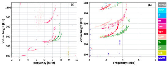
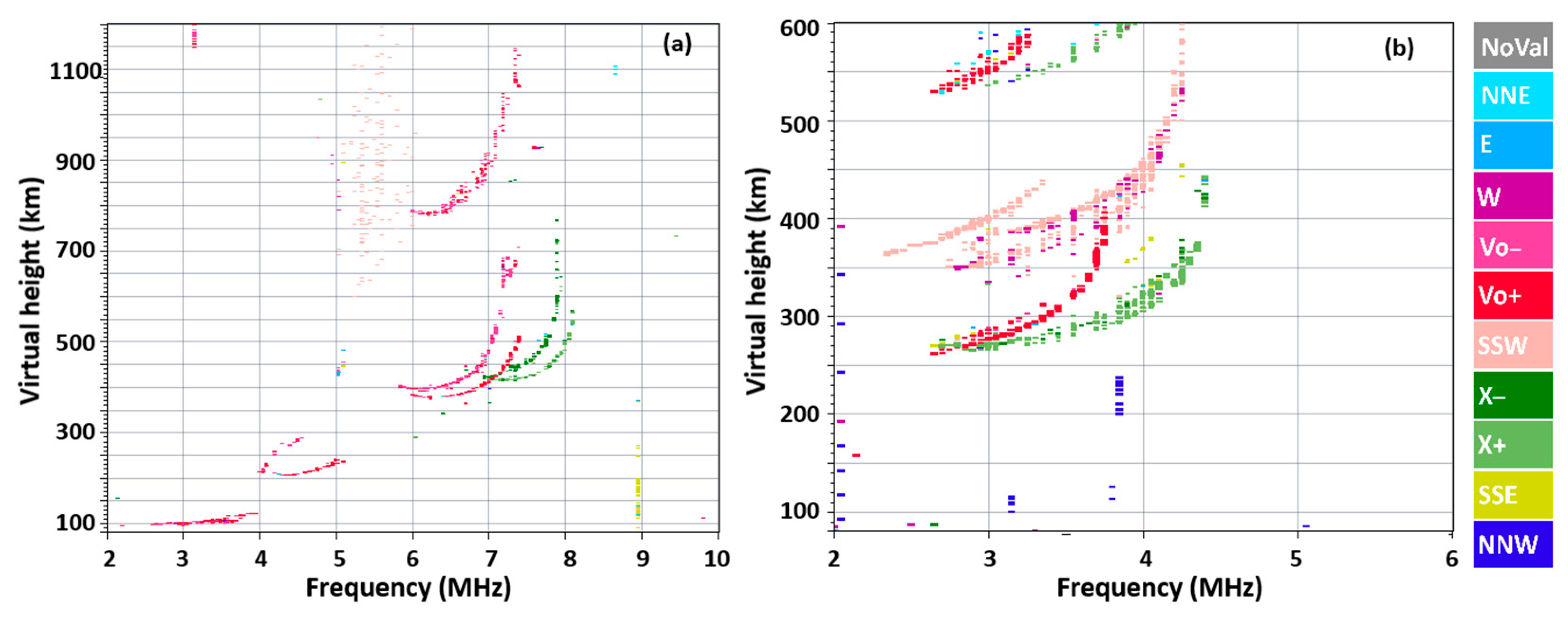
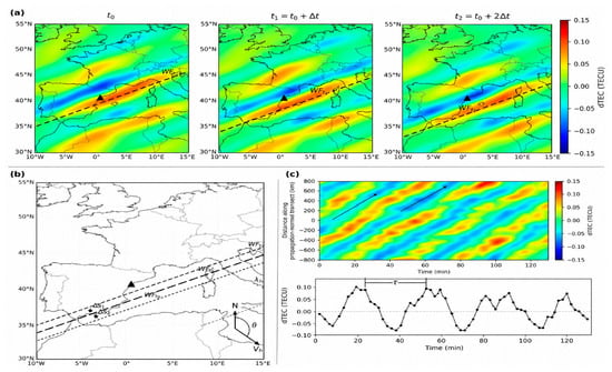
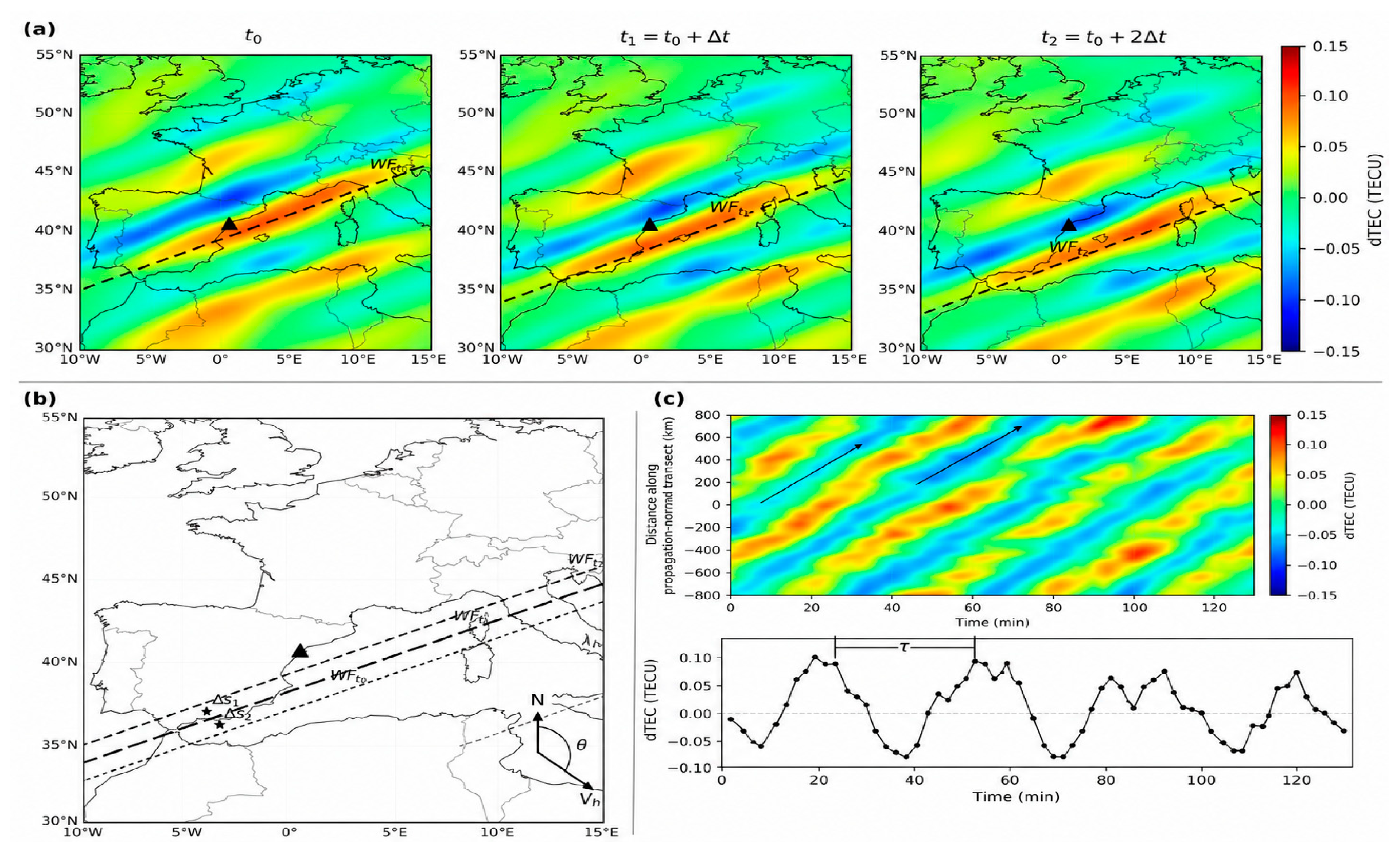
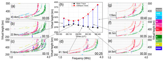
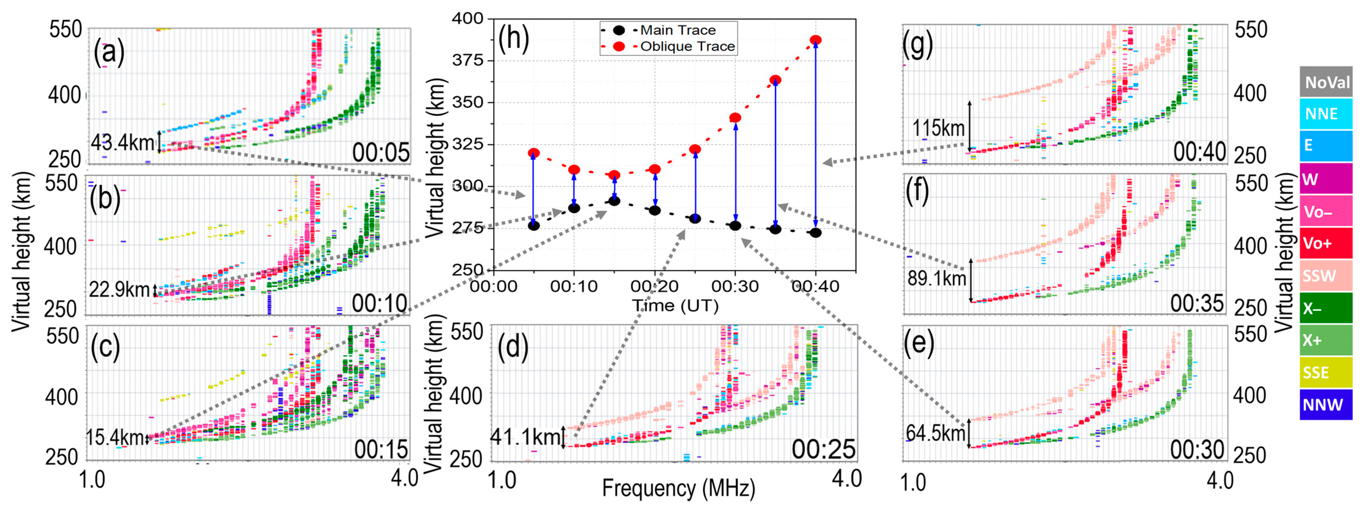
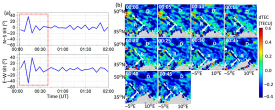
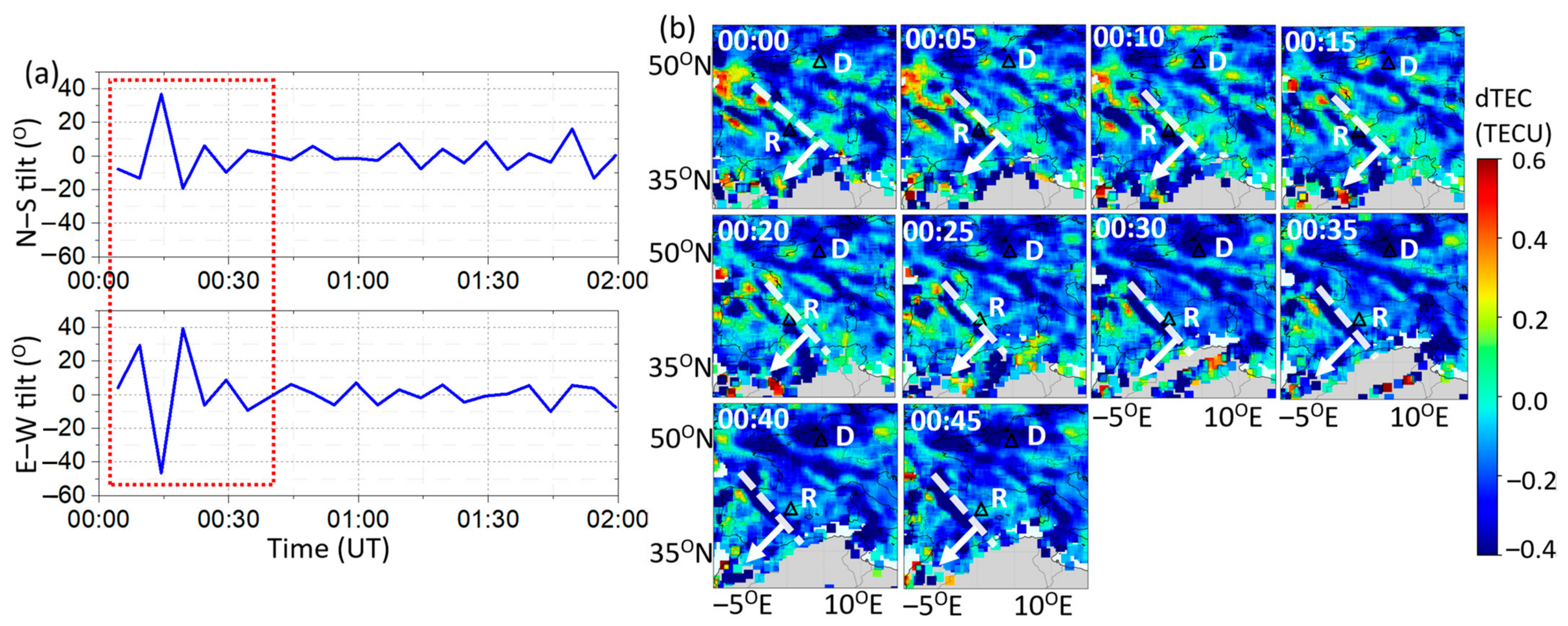
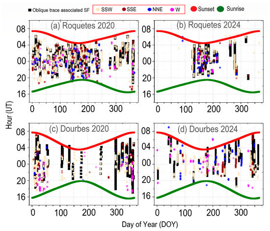
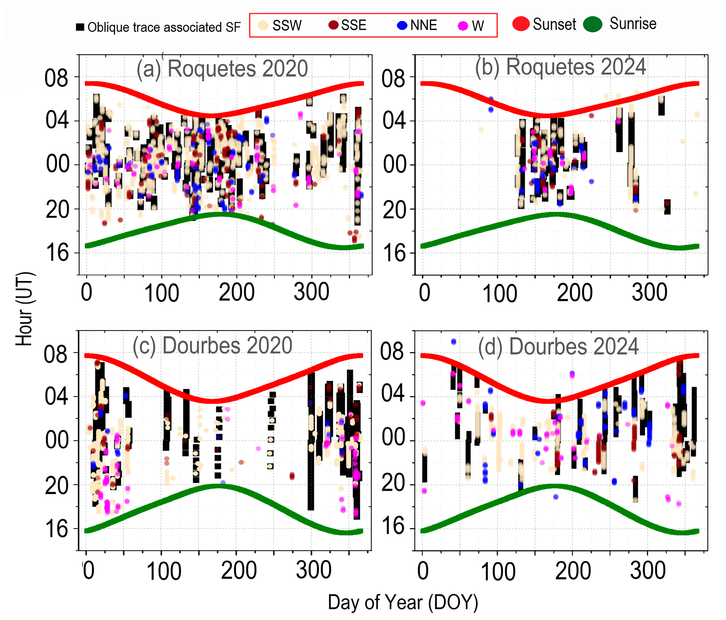
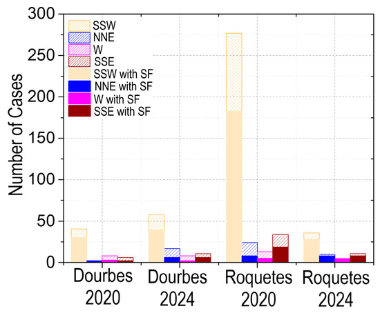
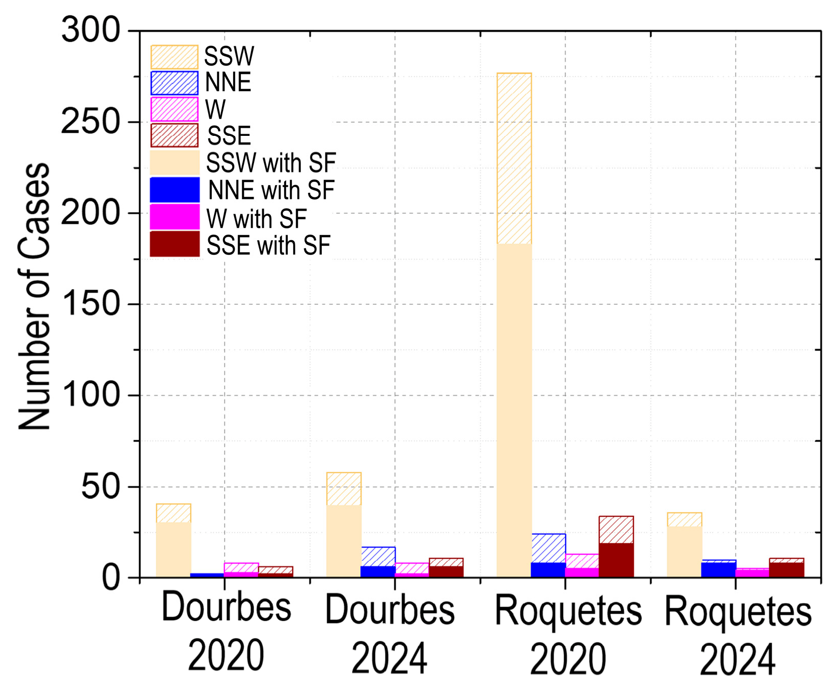
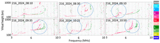
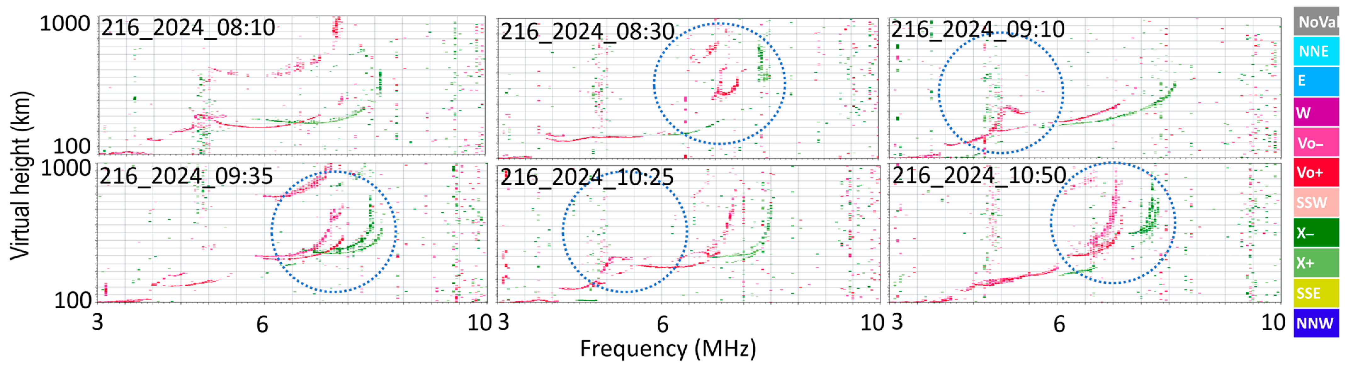
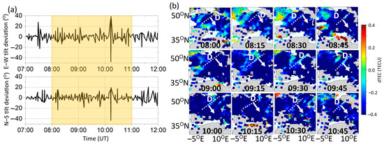
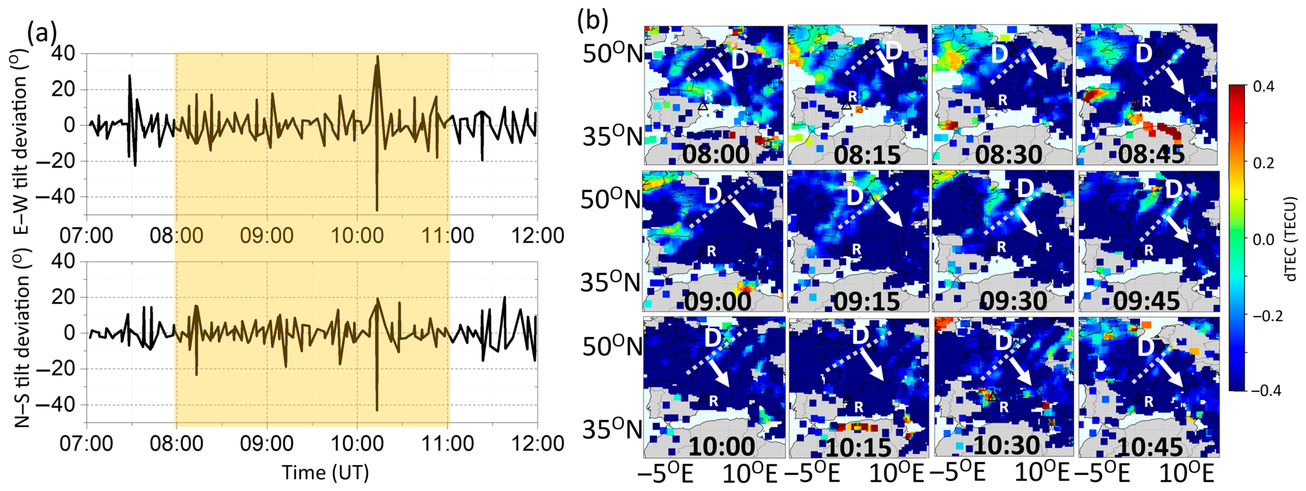
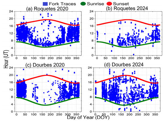
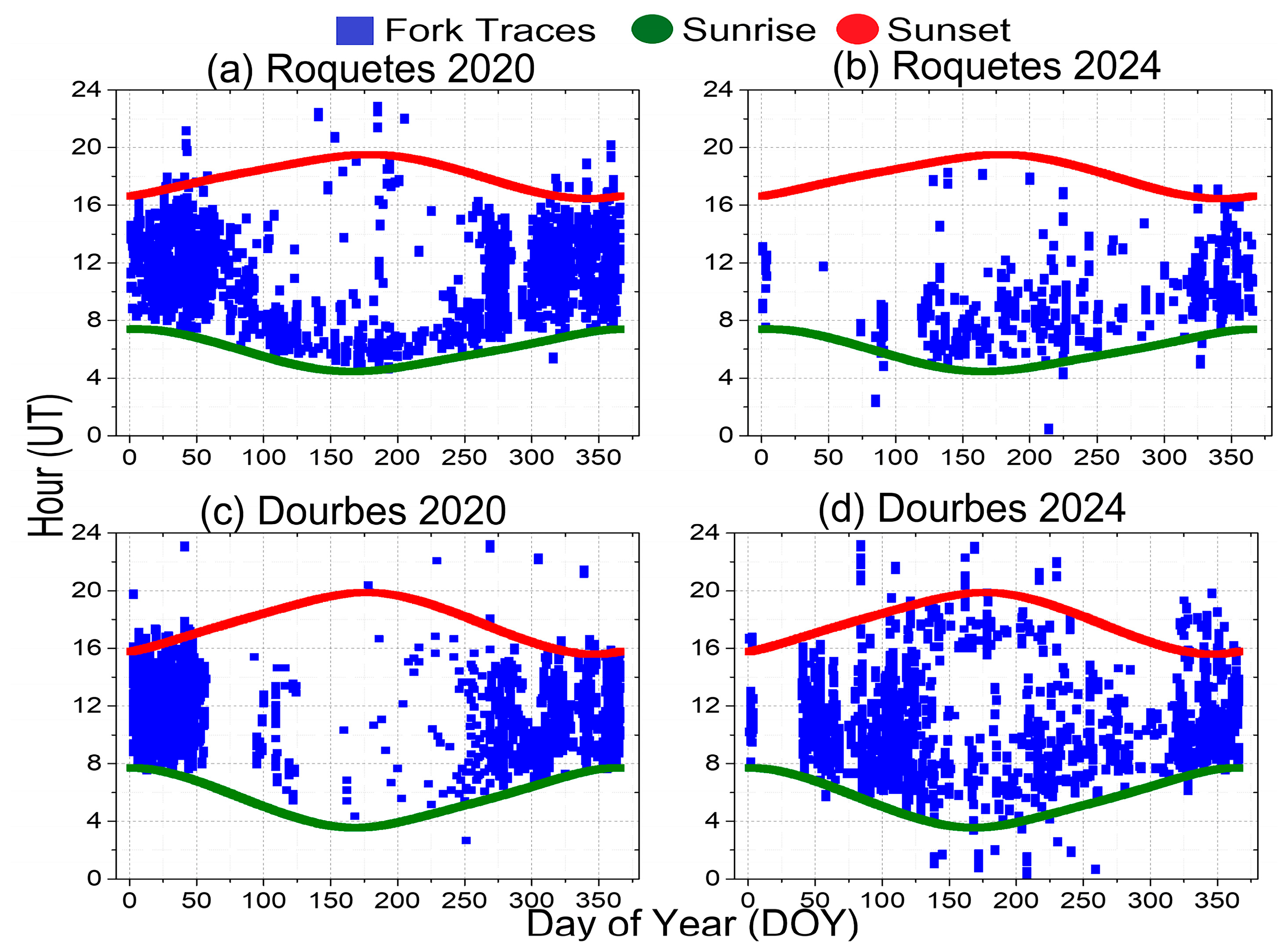
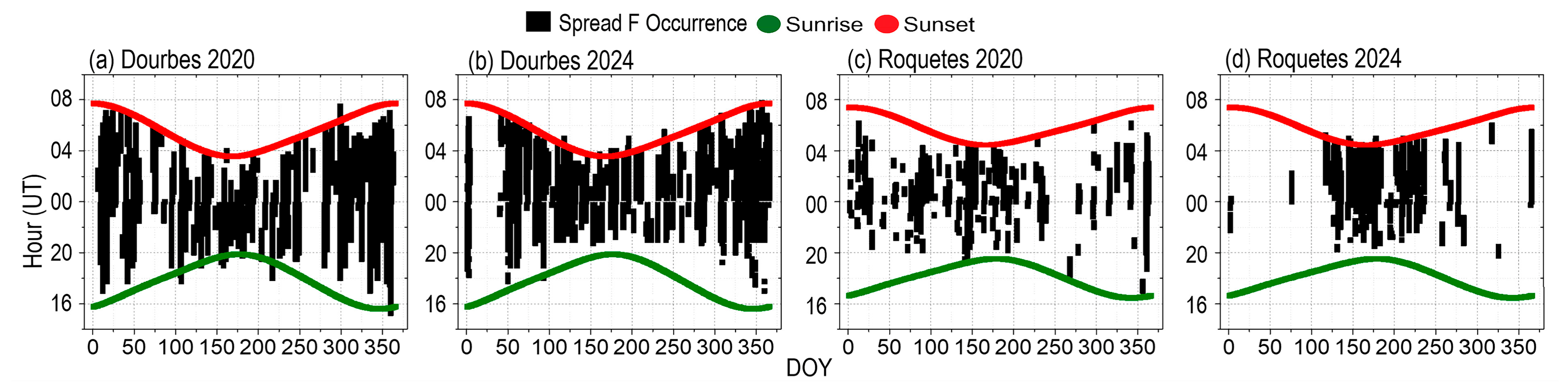
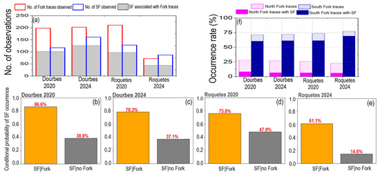
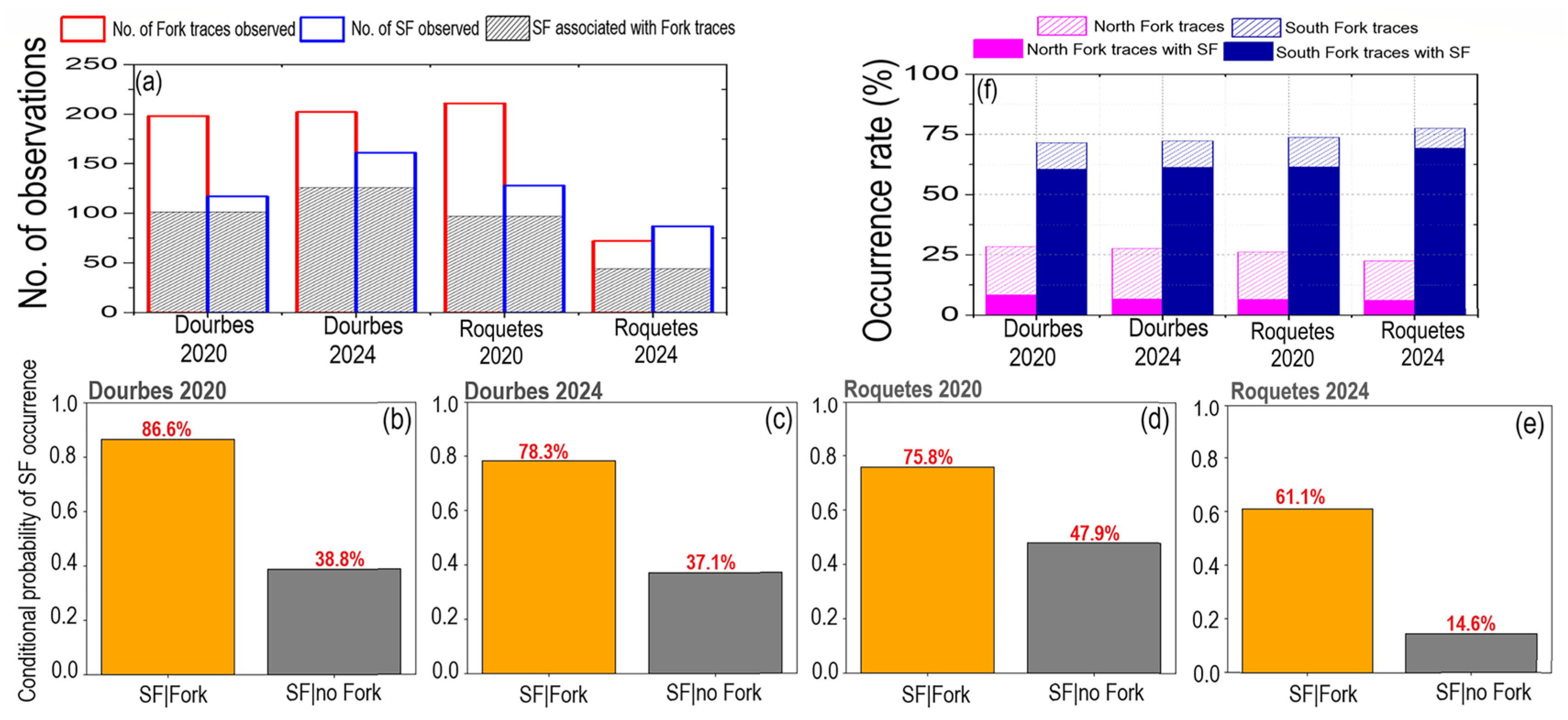
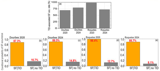
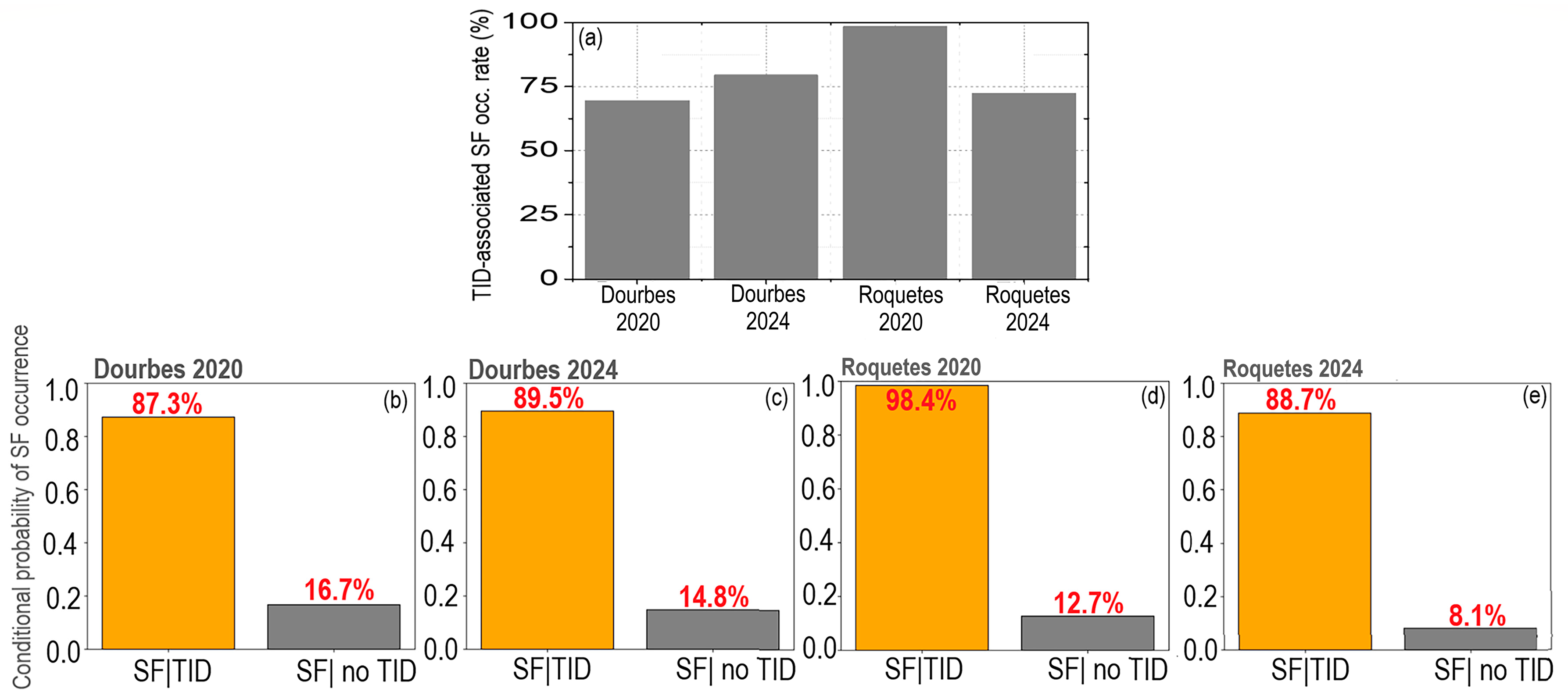
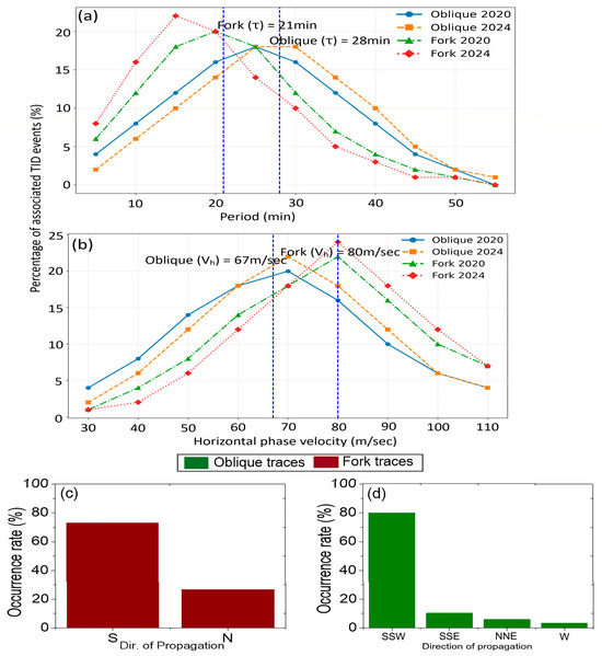
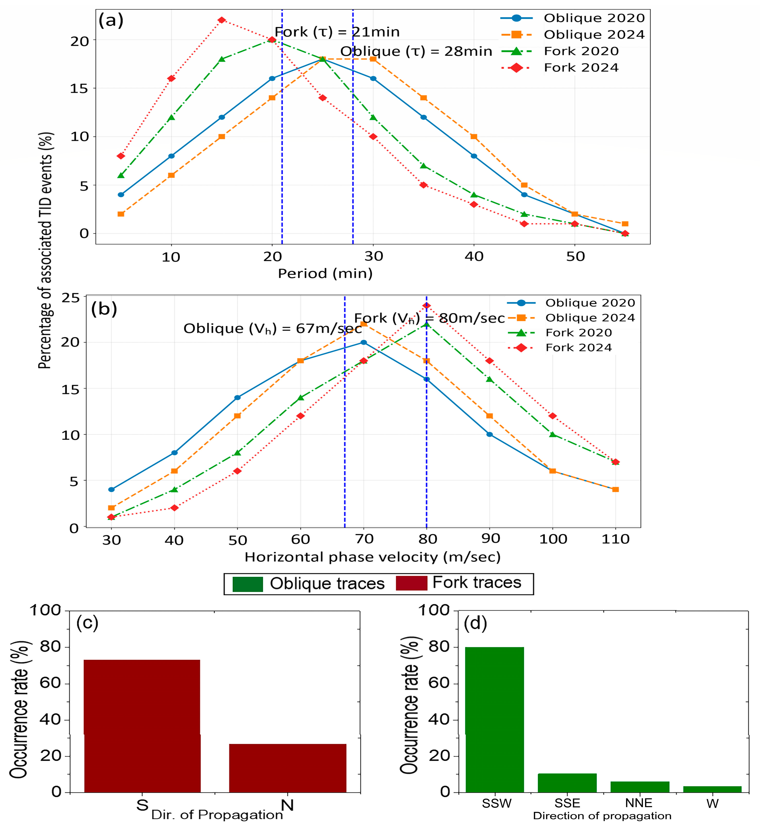
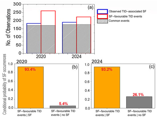
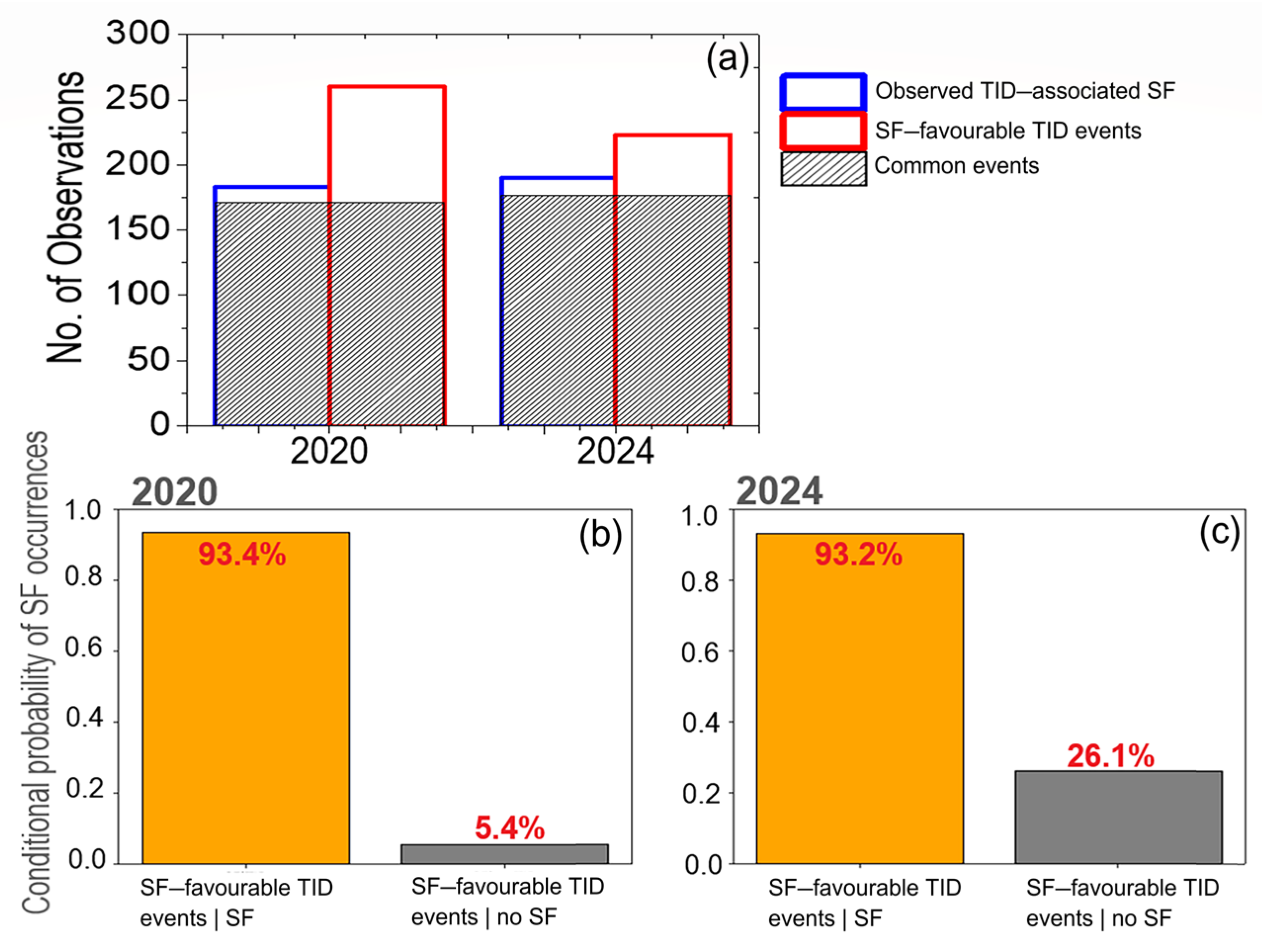

Disclaimer/Publisher’s Note: The statements, opinions and data contained in all publications are solely those of the individual author(s) and contributor(s) and not of MDPI and/or the editor(s). MDPI and/or the editor(s) disclaim responsibility for any injury to people or property resulting from any ideas, methods, instructions or products referred to in the content. |
© 2026 by the authors. Licensee MDPI, Basel, Switzerland. This article is an open access article distributed under the terms and conditions of the Creative Commons Attribution (CC BY) license.