A Validation of Temporal Downscaling Models of Estimating Hourly Temperatures Under South African Conditions

Abstract

High-resolution weather data is essential for studies related to fruit production, building sciences and other mathematical modelling. Most of the historical weather data prior to 1980 was mainly daily. The introduction of automatic weather stations led to the introduction of hourly, minute, and second interval weather data, depending on the period during which the measurement was conducted. In order to conduct studies on climate change and generate the Climate normal, at least 30 years of data is required, and for most of the stations in South Africa, which have long-term data, their normal period was from 1961 to 1990, and the new normal was from 1981 to 2010. It becomes difficult to use daily temperatures only to do analysis for studies that require hourly temperatures, such as the calculation or estimation of chill units or chilling hours. Therefore, there is a need to find a mathematical model or stochastically generating model to derive high temporal resolution temperature data. The temporal downscaling model was used to obtain a full record of hourly temperatures for the period 1981–2010. The validation was based on all winter days within this base period for which observed data were available. A sine curve with input parameters, including daily minimum and maximum temperatures, as well as the day of the year, was more suitable. Other models were also tested, and the results were similar. All the models performed very well under normal weather conditions, while all models failed to simulate the sudden disruption in temperature due to a cold front or any storm activity. Only models for weather forecasting are able to predict sudden changes, but the historical simulators failed, as their inputs were only the daily minimum and maximum, and there was no recording of hourly temperatures available.

1. Introduction

Daily weather variables, such as temperature, rainfall, relative humidity, wind speed, and solar radiation, are essential inputs for the analysis, simulation, and design of many engineering, biological, and agricultural systems [1,2,3]. The type and format of weather data required depend on the objectives of the study, the nature of the analysis, and the specific model being applied [3]. Among these variables, temperature is one of the most critical drivers of agricultural systems and a fundamental input for crop models used to analyse crop responses to climate variability and change [1].

In many cases, however, only daily minimum and maximum temperature data are available, particularly where observations were recorded manually at fixed times of the day (e.g., 08:00 and 14:00 local time). To address this limitation, methods have been developed to simulate hourly temperatures from daily minimum and maximum values, thereby enabling the use of extensive historical datasets [2]. Reconstructed diurnal temperature patterns are particularly useful as inputs to models simulating plant physiological processes, such as photosynthesis, transpiration, and crop development [4]. In addition, methods have been developed to estimate diurnal patterns of air temperature, wind speed, global radiation, and relative humidity from daily observations [4].

Numerous studies have investigated the modelling of hourly temperatures from daily, weekly, or monthly data [1,5,6,7]. For example, Richardson et al. [5] proposed a simple model for estimating hourly temperatures for the calculation of chill units, while [1] used a linear equation to represent the 12 h period between minimum and maximum temperature. Richardson, while applying this approach to estimate chill units, highlighted the limitations of assuming a symmetrical daily temperature curve and suggested that the interval between maximum and minimum temperatures should vary seasonally to better reflect changes in day length.

In a subsequent evaluation, Reicosky et al. [1] used independent hourly temperature observations collected over four years to validate five different methods that estimate missing hourly values from daily maximum and minimum temperatures. The study concluded that the model developed by [7], which used a cosine curve to describe the diurnal temperature cycle, produced the best performance. Under smooth diurnal temperature conditions, this model achieved a minimum root mean square error (RMSE) of 1.5 °C. Other approaches have also been explored, including the use of Fourier series [8], least-squares linear regression [9], and various temporal temperature downscaling models [6,10,11,12,13,14]. Most of these models employ modified sine functions to represent daytime heating [12].

Temperature plays a central role in biological development processes, with crop growth and phenology often being linearly related to thermal time accumulation [1]. While daily mean temperature influences overall crop growth and development, the diurnal temperature cycle is even more important because it affects plant morphological characteristics, such as leaf orientation, shoot growth, plant height, internode length, and nutrient balance [7]. Consequently, analysing crop responses to hourly temperature variations is more informative than relying solely on daily averages.

Most existing algorithms for downscaling daily temperature data to hourly values assign the daily maximum and minimum temperatures to specific times of the day and connect them using sinusoidal functions [2]. Such methods are particularly important in climate change research, where long-term historical datasets are required. Many temperature-based indices, including chill units, heat units, and phenological models, depend on hourly temperature data to capture diurnal temperature trends accurately [15].

In South Africa, a large proportion of historical weather observations from the 1960s to the 1990s were recorded manually, resulting in limited availability of continuous hourly temperature records. This study was therefore motivated by the lack of historical hourly data for the selected study sites during the 1980–1990 period. To overcome this limitation, temperature downscaling models were used to derive hourly temperature data from daily minimum and maximum observations. The main objective of the study was to generate hourly temperature datasets from daily temperature extremes and to evaluate the accuracy of the selected model in reproducing observed hourly temperature patterns [16].

2. Materials and Methods

2.1. Historically Observed Data

The historical climate data used in this study were obtained from two weather stations located in distinct climatic regions of South Africa. The datasets represent observations collected from two generations of weather monitoring systems. During the early 1980s, weather observations were recorded manually at specific times of the day, whereas later records were obtained from automated weather stations.

Daily and hourly temperature data for Bethlehem and Upington (Table 1) were acquired from the South African Weather Service (SAWS). For Bethlehem, hourly temperature observations were available from 1980, while historical records dating back to 1969 contained measurements at selected observation times (08:00, 12:00, 14:00, 16:00, and 20:00). In Upington, continuous hourly observations became available from 1980 following the installation of automatic weather stations. Gaps in the observational record can be supplemented using weather generators or temperature simulation models, thereby enabling the reconstruction of continuous hourly datasets for periods where observations are unavailable.

Table 1. Climate summary for the period 1981–2010 for the two study sites [17].

				Mean	Average Temperature (°C)
Area	Latitude (S)	Longitude (E)	Altitude (m)	Annual	Maximum	Minimum
				Rainfall (mm)	January July	January July
Bethlehem	28°20′	28°15′	1680	680	27.2 16.4	13.2 −2.0
Upington	21°15′	28°24′	840	94	35.5 20.8	19.8 4.1

The analyses were conducted separately for each month of the year, as the performance of temperature reconstruction algorithms may vary seasonally. Different modelling approaches were evaluated and compared. The Sinusoidal and Parabolic methods [1] generally assume a sinusoidal temperature curve during the daytime and a separate function for nighttime cooling. While these approaches are computationally simple and widely applied, they may perform poorly during overcast conditions or periods characterised by abrupt weather changes.

The Wave Model [16,18] was also evaluated to determine its ability to capture sudden temperature fluctuations associated with synoptic weather systems such as cold fronts. Unlike conventional temperature reconstruction methods, artificial intelligence (AI) and machine learning approaches are capable of identifying complex, non-linear relationships and anomalous patterns within climatic datasets. Although these methods have demonstrated high predictive accuracy in weather forecasting applications, often achieving concordance correlation coefficients exceeding 90%, their primary strength lies in forecasting future conditions rather than reconstructing observed hourly temperatures from daily summary statistics [18]. Nevertheless, AI-based methods have shown promise in accounting for regional climatic variability and non-idealised temperature patterns that are difficult to represent using traditional deterministic approaches.

The performance of the temperature reconstruction algorithms was evaluated using several statistical measures. Daily maximum and minimum temperature observations from the period of 1981 to 2010 were extracted from the historical records and used as inputs to generate hourly temperature values using each of the selected algorithms. The generated hourly temperature datasets were then compared with observed hourly temperatures using three complementary approaches:

• Root Mean Square Error (RMSE): To quantify the overall magnitude of prediction errors between observed and simulated hourly temperatures.
• Cumulative Temperature Comparison: To assess differences between observed and simulated cumulative temperature values over time, which is particularly important for applications such as chilling accumulation, heat unit calculations, and crop phenology modelling.
• Average Hourly Temperature Profiles: To evaluate the ability of each algorithm to reproduce the observed diurnal temperature cycle and hourly temperature patterns.

These evaluation procedures provided a comprehensive assessment of the accuracy and reliability of each model across different climatic regions and seasons, enabling the identification of the most suitable approach for generating hourly temperature data from daily temperature observations.

The assumptions

The assumption made in this study is that for all the models used, the only input available is the daily minimum and maximum temperatures. The models are only simulating the diurnal hourly temperatures from the two inputs, and also the day length and the seasonal distinction of sunrise and sunset times during winter months and summer months. The paper is a chapter from the unpublished work, which was conducted during the period 2011 to 2014, which explains the reason behind the choice of data range of 1981 to 2010.

2.2. Temporal Downscaling Model

The process of deriving hourly temperature values from daily minimum and maximum temperatures is far from straightforward, as demonstrated by numerous studies on this subject [1,2,3,5,12,19,20]. Diurnal temperature variation is governed by a complex interaction of atmospheric and surface processes, including day length, air moisture content, cloud cover, wind speed, precipitation events, the movement of air masses, proximity to high- and low-pressure systems, soil heat flux, and evaporative cooling from the land surface.

Most temporal downscaling models (TDMs) are based on the assumption that daily minimum and maximum temperatures occur at relatively consistent times of the day, with minimum temperatures typically occurring during the early morning and maximum temperatures during the afternoon. However, these assumptions are not always valid under real-world conditions. For example, the passage of a cold front during the morning hours may result in the daily maximum temperature occurring earlier than expected, rather than during the afternoon period [21]. Similarly, the daily minimum temperature may occur later in the day under certain weather conditions.

The timing of observations can also influence historical temperature records, particularly when data are collected manually at fixed observation times [22]. In some instances, temperatures may not exceed or fall below those recorded at the previous observation time, causing the reported 24 h maximum or minimum temperature to correspond to the preceding day. Although it is impossible to control the natural timing of temperature extremes, the use of 12 h maximum and minimum temperature observations can help reduce errors associated with observation timing and improve the reliability of reconstructed hourly temperature profiles.

A sinusoidal function is often considered an appropriate representation of the daytime temperature curve because air temperature closely follows the daily cycle of incoming solar radiation. The cooling phase during the night, however, is considerably more complex and is influenced by several environmental factors, including atmospheric moisture, cloud cover, wind conditions, and soil heat exchange processes. Consequently, various approaches have been proposed to represent nocturnal cooling.

For example, Parton and Logan [23] suggested a cooling function based on the square root of the elapsed time since sunset, while another formulation by [23] employed an exponential decay function to describe nighttime cooling rates. Eckersten [24] modified the model developed by Parton and Logan into a sine–sine exponential formulation, resulting in improved representation of the cooling period between daily maximum and minimum temperatures. Similarly, Linvill [2] adopted a sine–sine approach to describe both daytime heating and nighttime cooling and incorporated a logarithmic function to represent nocturnal temperature decline.

The temperature wave model proposed by [2,3] was adopted in this study to reconstruct hourly temperature values from daily temperature observations. This approach combines concepts from several earlier models [1,5,6,7] to provide a relatively simple yet robust method for estimating hourly temperatures, particularly for applications such as chill unit calculations and crop modelling. The model assumes that the daily maximum temperature occurs approximately two hours after solar noon and that the daytime temperature curve follows the pattern of the solar radiation cycle. Under these assumptions, the temperature wave between sunrise and sunset can be represented using a sinusoidal function that describes the daytime heating process. The mathematical formulation of the model used to estimate hourly temperatures during the daylight period is presented in the following section.

$$\mathrm{T}\left(\mathrm{t}\right)=\left({\mathrm{T}}_{\mathrm{m}\mathrm{a}\mathrm{x}}-{\mathrm{T}}_{\mathrm{m}\mathrm{i}\mathrm{n}}\right)\times \sin \left[{\displaystyle \frac{\mathsf{\pi }\mathrm{t}}{\mathrm{D}\mathrm{L}+4}}\right]+{\mathrm{T}}_{\mathrm{m}\mathrm{i}\mathrm{n}}$$

(1)

where T(t) is the temperature (in °C) at time t after sunrise;

T_max is the maximum temperature (in °C);

T_min is the minimum temperature (in °C);

DL is the day length (in hours).

The temperature at sunrise was set equal to the observed minimum temperature for the day. A second expression was used to define nighttime cooling starting after sunset. Minimum daily temperatures were thus reached near the time of sunrise [2,3]:

$$\mathrm{T}\left(\mathrm{t}\right)={\mathrm{T}}_{\mathrm{s}}-{\displaystyle \frac{{\mathrm{T}}_{\mathrm{s}}-{\mathrm{T}}_{\mathrm{m}\mathrm{i}\mathrm{n}}}{\mathrm{l}\mathrm{n}(24-\mathrm{D}\mathrm{L})}}\times \ln \left(\mathrm{t}\right)$$

(2)

where T(t) is the temperature at time t > 1 h after sunset;

T_{s is} the sunset temperature (in °C);

T_min is the minimum temperature on the following morning (in °C).

The day length (DL) was calculated from the following algorithm developed by Stuff and Dale (1973), and cited by [2]:

$$\mathrm{C}\mathrm{D}=\mathrm{I}\mathrm{N}\mathrm{T}\mathrm{E}\mathrm{G}\mathrm{E}\mathrm{R}(30.6\times \mathrm{M}\mathrm{O}\mathrm{Y}+\mathrm{D}\mathrm{O}\mathrm{M}-91.3)$$

(3)

$$\mathrm{D}\mathrm{L}=12.25+3.34\times \mathrm{t}\mathrm{a}\mathrm{n}\mathrm{\varnothing }\times \mathrm{c}\mathrm{o}\mathrm{s}(0.0172\times \mathrm{C}\mathrm{D}-1.95)$$

(4)

where CD is the climatological day number (numbered from 1 March);

MOY is the month of the year;

DOM is the day of the month;

Ø is the latitude (in °) with Ø < 0 in the southern hemisphere.

A computational problem arose with respect to the first hour after sunrise, which was never clarified in [2,3]. As stated correctly, the nighttime cooling curve (Equation (2)) calculates the temperature T(t) at time t > 1 after sunset, implying it cannot be used when t = 1 h after sunset, as this setting yields the same value as for the sunset hour. Simply applying the daytime curve (Equation (1)) for another hour after sunset was not an option either, as this was not its intended purpose or resulted in irregular cooling (viz. a perturbation in the cooling portion of the curve). The Southern Hemisphere experiences different seasons, and during those seasons, the sunset happens at different times. The reason for altering the equation for T = 1 to T = 1.5 for the first hour after sunrise is due to the changes in the sunset time and sunrise during the winter season, as compared to the summer season, wherein the sun rises earlier, of which the model will use 1 h after sunrise and in winter will be delayed by half an hour. The data used for the study was collected during the winter period.

TDMs have limitations in real-world systems, and they hardly imitate the exact real-world system. Therefore, any model should be validated to the degree needed for the model’s intended purpose [25]. Chow and Levermore [26] found that it is important to measure the significance of various conventional downscaling procedures and to determine whether they are acceptable for use in validation.

2.3. Validation of the Model

Validation of the model was performed for two stations in South Africa, falling in different climate regions, for which hourly temperature records were available. The coefficients of the recommended model were determined using the hourly data observed during at least 30 years between 1981 and 2010.

The choice of statistical metrics was based on the literature and previous studies performed on the validation of models [1,2,3,12,26,27,28]. The “goodness of fit” measures used to validate the TDM included mean absolute error (MAE), root mean square error (RMSE), coefficient of determination (R²) and Model Efficiency (ME). The statistics such as RMSE and MAE have been used as standard statistical metrics to measure the model performance in meteorology, air quality and climate research studies [29]. In addition to these standard measures, graphs such as scatter plots, histograms and cumulative distribution functions were also used to judge model error subjectively.

2.3.1. Mean Absolute Error (MAE)

The MAE is defined as the sum of the absolute values of the difference between the predicted and observed temperature within the validation period [30]. The MAE is a linear score, meaning that all individual differences are weighted equally [31]. It measures the accuracy for continuous variables and is given by the following:

$$\mathrm{M}\mathrm{A}\mathrm{E}={\displaystyle \frac{1}{\mathrm{n}}}{\displaystyle {\sum }_{\mathrm{i}=1}^{\mathrm{n}}}\left|{\mathrm{x}}_{\mathrm{i}}-{\mathrm{y}}_{\mathrm{i}}\right|={\displaystyle \frac{1}{\mathrm{n}}}{\sum }_{\mathrm{i}=1}^{\mathrm{n}}\left|{\mathrm{e}}_{\mathrm{i}}\right|$$

(5)

where n is the number of observations;

y is the predicted temperature;

x is the observed temperature at any time.

The MAE can range from 0 to ∞. The lower the value of MAE, the better the accuracy of the model. The MAE is appropriate in describing uniformly distributed errors [29].

2.3.2. Root Mean Square Error (RMSE)

The RMSE is a quadratic scoring rule, which measures the average magnitude of the error [30]. Each value (hourly or daily temperature) generated by the model, y, is compared to the corresponding value from the real observed dataset, x. For n entries, the RMSE is given by the following:

$$\mathrm{R}\mathrm{M}\mathrm{S}\mathrm{E}=\sqrt{{\displaystyle \frac{{\displaystyle {\sum }_{\mathrm{i}=1}^{\mathrm{n}}}{({\mathrm{x}}_{\mathrm{i}}-{\mathrm{y}}_{\mathrm{i}})}^2}{\mathrm{n}}}}$$

(6)

where n is the number of observations;

x is the observed temperatures;

y is the predicted temperatures.

The RMSE is used to diagnose the variation in the errors of the predicted values. The RMSE ranges from 0 to ∞. Small RMSE values are desirable. The underlying assumption of the RMSE is that the errors are unbiased and follow a normal distribution [29].

2.3.3. Coefficient of Determination (R²)

The R² conveys information on whether it is possible to predict the future outcomes of a variable on the basis of the given information [32,33]. It provides a measure of how well future outcomes are likely to be predicted by the regression function. It can be defined as the variation in the dependent variable that can be explained by the regression line and the corresponding independent variable(s). The R² is given by the following:

$${\mathrm{R}}^2={\left[{\displaystyle \frac{1}{\mathrm{n}}}{\displaystyle \frac{\sum \left(\mathrm{x}-\overline{\mathrm{x}}\right)\left(\mathrm{y}-\overline{\mathrm{y}}\right)}{{\mathsf{\sigma }}_{\mathrm{x}}{\mathsf{\sigma }}_{\mathrm{y}}}}\right]}^2$$

(7)

where n is the number of observations;

$\overline{\mathrm{x}}$ is the mean of the observed values;

$\overline{\mathrm{y}}$ is the mean of the predicted values;

σ_x is the standard deviation of the x values;

σ_y is the standard deviation of the y values.

The R² provides information regarding the goodness of fit of a model, and it measures how well the regression line approximates the observed data [34]. R² is bounded by 0 ≤ R² ≤ 1 and can thus never be negative. An R² of 1 indicates that the regression line perfectly fits the data, whereas an R² value of 0 is indicative of a useless model.

2.3.4. Model Efficiency (ME)

The ME is commonly used to assess the predictive power of prediction models [35]. However, it can also be used to quantitatively describe the accuracy of model outputs (such as discharge nutrient loadings, temperatures and concentrations). In addition, ME measures how well a model reproduces measured data. It is given by the following:

$$\mathrm{M}\mathrm{E}=1-{\displaystyle \frac{{\displaystyle {\sum }_{\mathrm{i}=1}^{\mathrm{n}}}{({\mathrm{x}}_{\mathrm{i}}-{\mathrm{y}}_{\mathrm{i}})}^2}{{\displaystyle {\sum }_{\mathrm{i}=1}^{\mathrm{n}}}{({\mathrm{x}}_{\mathrm{i}}-\overline{\mathrm{x}})}^2}}$$

(8)

where n is the number of observations;

x is the observed values;

y is the predicted values;

$\overline{\mathrm{x}}$ is the mean of observed values.

ME can range from −∞ to 1. If ME = 1, the model produces an exact prediction for each data point. A zero value of ME implies that a single measured mean is as good an overall predictor as the model. A negative value of ME indicates that the measured mean is a better predictor than the model. Essentially, the closer the model’s efficiency is to 1, the more accurate the model.

The TDM was consequently used to obtain a full record of hourly temperatures for the period 1981–2010. The validation was based on all winter days within this base period for which observed data was available. Gaps in the data for Upington were encountered for the months of August 1989 and June 1992, which were subsequently omitted from the validation process.

2.4. The Wave Model

In this study, three regression models (linear, polynomial, and logistic) and the modified WF model were investigated to determine the model accuracy used to calculate hourly water temperature in a river from hourly air temperature. The linear regression model is the simple regression model shown as Equation (2), which was used in many previous studies for daily or weekly temperature regressions [9,14]; the polynomial regression model uses the second-order polynomial defined by Equation (9):

$${\mathrm{T}}_{\mathrm{w}}\left(\mathrm{t}\right)=\mathrm{c}\mathrm{c}·{\mathrm{T}}_{\mathrm{a}}(\mathrm{t}{)}^2+\mathrm{d}·{\mathrm{T}}_{\mathrm{a}}\left(\mathrm{t}\right)+\mathrm{f}$$

(9)

where Tw(t) is the hourly water temperature;

Ta(t) is the hourly air temperature with or without lag; a, b, c, d and f are regression coefficients. Water temperatures calculated from the linear model follow diurnal variations in hourly air temperatures. The coefficients a and b in Equation (9) are scale and translation parameters. When the polynomial regression model is used, the scale and translation from air temperature to water temperature are nonlinear. The logistic regression model has been used over the last few decades to develop air and water temperature relationships [36], and it is a four-parameter model defined using Equation (10):

$${\mathrm{T}}_{\mathrm{w}}=\mathsf{\mu }+{\displaystyle \frac{\mathsf{\alpha }-\mathsf{\mu }}{1+{\mathrm{e}}^{\mathsf{\gamma }(\mathsf{\beta }-{\mathrm{T}}_{\mathrm{a}})}}}$$

(10)

where μ (°C) is a coefficient that estimates minimum water temperature, α (°C) is a coefficient that estimates maximum water temperature, γ (dimensionless) represents the steepest slope (inflection point) of the logistic Tw function when plotted against Ta, and β (°C) is the air temperature at the inflection point. The diurnal variations in water temperature curves are a combination of periodic sine and exponential decay functions [2]. The wave model was initially presented by [16], and Reicosky et al. [1] used the sinusoidal to estimate hourly air temperatures using daily maximum and minimum air temperatures as input. It was obtained from the subroutine wave model in [7]. In this study, the wave model, as the fourth model, was used to estimate hourly water temperatures using daily maximum and minimum water temperatures as input. To predict hourly air temperatures, Reicosky et al. [1] assumes that the maximum air temperature is at 14:00 h and the minimum air temperature is at sunrise for each day, which is embedded in the guidelines of the World Meteorological Organization (WMO). Considering the time lag of water temperatures from air temperatures [14], the times of maximum and minimum water temperatures should be set differently from the times for maximum and minimum air temperatures.

For the modified WF model based on the WF used in previous studies [16,37,38], the intervening temperatures at time H hour (0:00 to 24:00 h) are calculated from the following equations: for 0 ≤ H < (RISE + 2) and 16:00 h < H ≤ 24:00 h,

TW(H) = TWAVE + AMP (cos (π H’/(10 + RISE)))

(11)

$$\mathrm{T}\mathrm{w}\left(\mathrm{H}\right)=\mathrm{T}\mathrm{w}\mathrm{a}\mathrm{v}\mathrm{e}+\mathrm{A}\mathrm{m}\mathrm{p}\left(\mathrm{C}\mathrm{o}\mathrm{s}\right({\displaystyle \frac{\mathsf{\pi }\mathrm{H}}{\left(10+\mathrm{R}\mathrm{i}\mathrm{s}\mathrm{e}\right)}}\left)\right)$$

(12)

For (RISE + 2) ≤ H ≤ 16:00 h,

TW(H) = TWAVE − AMP (cos (π ((H − RISE − 2)/(16 − RISE − 2)))

(13)

$$\mathrm{T}\mathrm{W}\left(\mathrm{H}\right)=\mathrm{T}\mathrm{w}\mathrm{a}\mathrm{v}\mathrm{e}-\mathrm{A}\mathrm{M}\mathrm{P}\left(\cos \left(\mathsf{\pi }\right({\displaystyle \frac{(\mathrm{H}-\mathrm{R}\mathrm{i}\mathrm{s}\mathrm{e}-2)}{(16-\mathrm{R}\mathrm{i}\mathrm{s}\mathrm{e}-2)}}\right)\left)\right)$$

(14)

where RISE is the time of sunrise in hours in each day and TW(H) is the water temperature at time H hour, H’ = H + 8 if H < (RISE + 2), H’ = H − 16 if H > 16:00 h, and TWAVE and AMP are defined as TWAVE = (TWMIN + TWMAX)/2 as the daily mean temperature and AMP = (TWMAX − TWMIN)/2 as temperature amplitude. TWMAX and TWMIN are estimated daily maximum and minimum water temperatures from logistic regressions using daily maximum and minimum air temperatures as input.

3. Results

Validation of the Temporal Downscaling Model

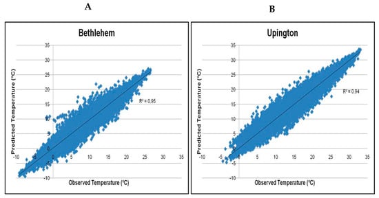
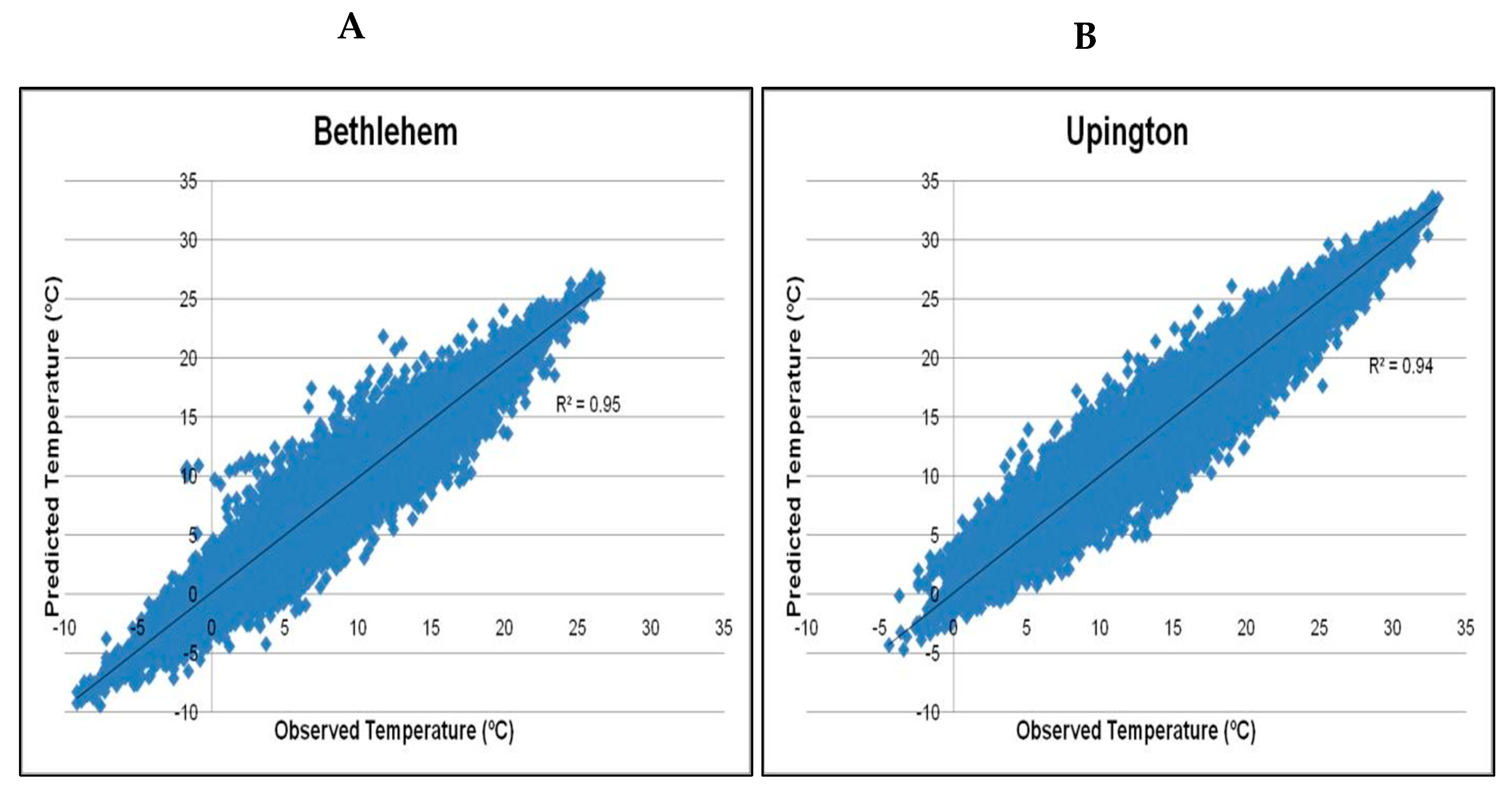
A very good fit is crucial, as the TDM was developed specifically to operate at high-resolution time scales. Table 2 contains a summary of the validation statistics for the selected days. In general, the TDM performed exceptionally well with R² values above 0.94 (Figure 1). The amount of data used for the validation is for all the hours from 1981 to 2010, which generates a good fit due to the amount of data, and therefore, sudden changes in weather were not factored in. The statistical results show a good correlation between the observed and the modelled data, which provides confidence in the use of these models. The models must always be used bearing the assumptions in mind that there will be no sudden changes in temperatures. All the days are assumed to have been clear skies and calm, from low temperatures during sunrise and reaching a peak during the day, and declining again towards sunset and overnight, with continuous decline.

Table 2. Validation statistics for hourly temperature predicted by the temporal downscaling model for selected weather stations for Short term Data sets.

Areas	MAE	RMSE	R2	ME
Bethlehem	1.18	1.61	0.95	0.94
Upington	1.22	1.63	0.94	0.95
Cold front Day (Bethlehem)	1.02	1.24	0.68	0.66

MAE = mean absolute error, R² = coefficient of determination, RMSE = root mean square error.

Figure 1. Scatterplot of observed against predicted hourly temperatures for Stations (A) and (B).

Table 2 shows the goodness of fit measures obtained when validating the TDM for two manual weather stations. The MAEs were between 1.18 and 1.22, whilst RMSEs were in the range of 1.61 and 1.63 for both stations. R² was equal to 0.95 and 0.94 (Table 2 and Figure 1). This means that the TDM used generally represented the measured data satisfactorily, and the correlation was very good. During the day of the cold front, the statistical analysis indicates that there was a decline in the correlation and the RMSE had a low value of 1.24 °C, as compared to the data during a normal day for the Bethlehem Station. The R² value was low and showed less correlation.

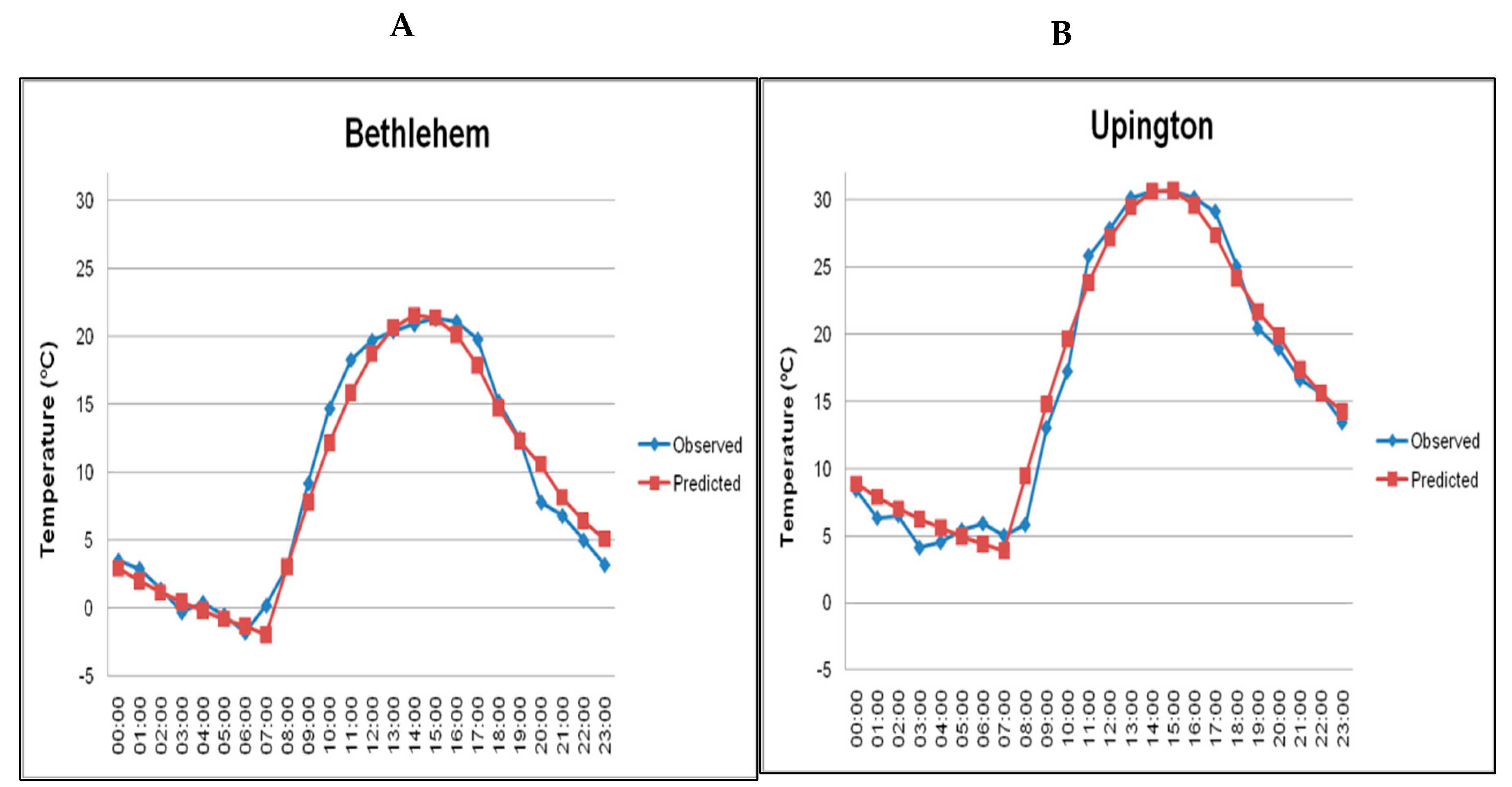
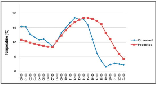
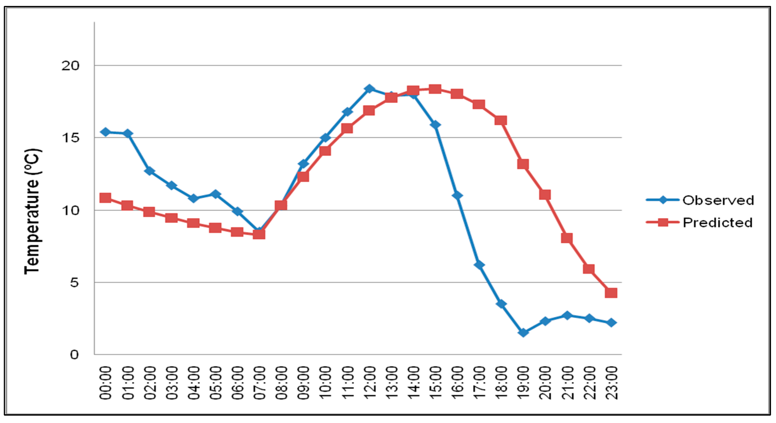
The temperature curves presented in Figure 2 for a randomly selected day within the validation period indicate a close correspondence between the observed and TDM-derived hourly temperatures at both sites. An investigation into some of the outliers in Figure 1 revealed that these were likely produced by the TDM failing to simulate sudden temperature changes associated with frontal passages. An example of such a case is presented in Figure 2, where a cold front moved over Bethlehem during the afternoon of 27 August 1996. It can be seen that the daytime curve faired reasonably well until the time of frontal passage (approximately 14:00 local time), where after, the observed temperature dropped abruptly, resulting in an increase in the forecast error until the nighttime cooling curve converged towards the next morning’s.

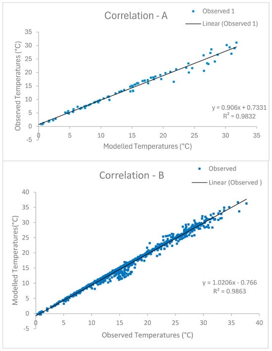
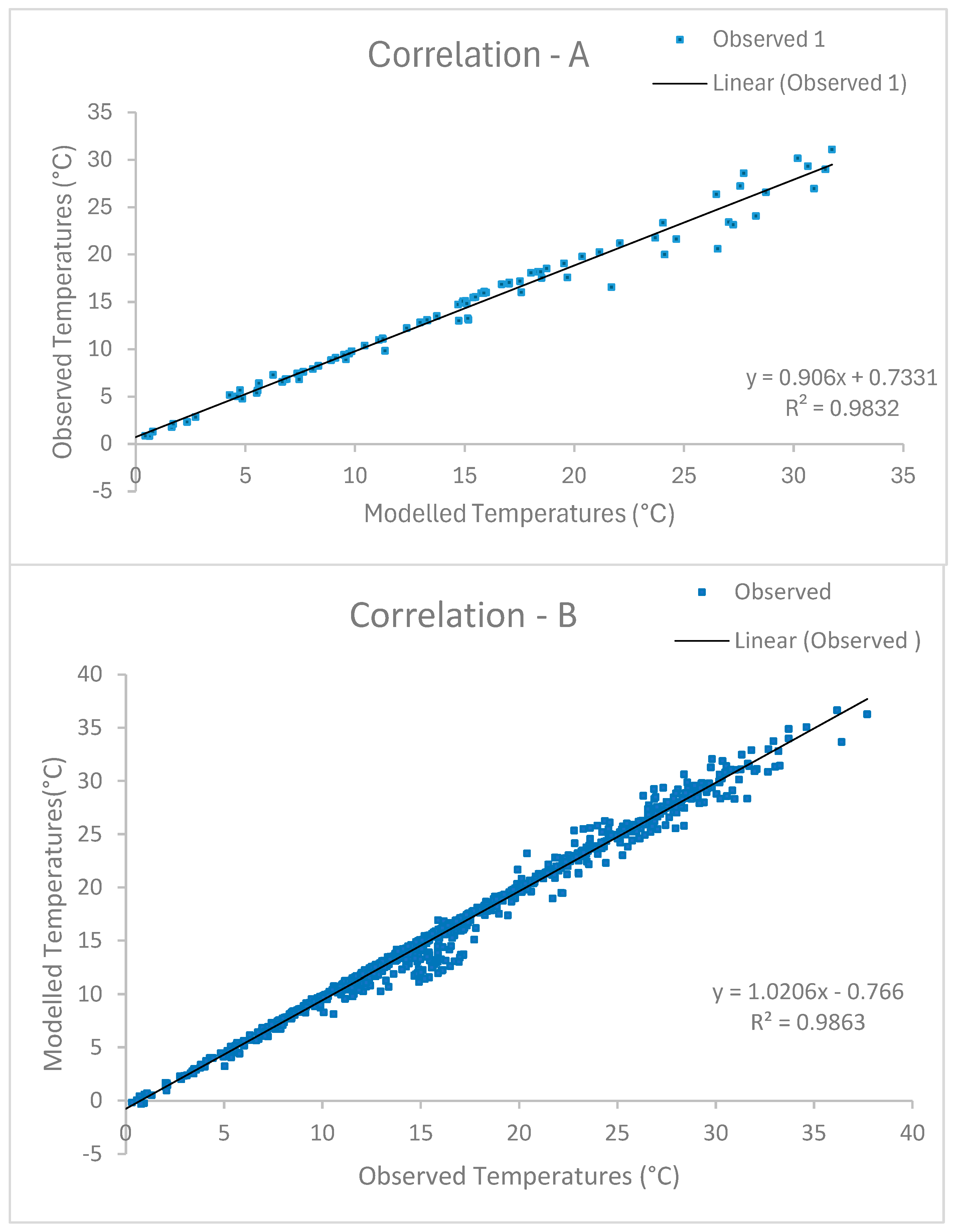
Figure 2. The correlation between the modelled temperature data and the observed hourly temperature data from the wave model algorithm for short term data (A) and long-term data (B).

The correlation between modelled data using a very few number of days shows a good correlation, and the outliers are only on the day where there was a sudden change in temperature due to the passing of a cold front (Figure 2). The correlation of modelled temperature from the wave model algorithm for more days does not show the outliers, as it shows a positive correlation. Figure 2 show graphic examples of linear and logistic regression models between hourly observed temperatures and hourly modelled air temperatures in Bethlehem. Table 3 gives a statistical summary of times or hours of maximum and minimum water temperatures. The average improvement in RMSE (Table 3) for linear regression with a time lag is approximately 0.3 °C. Morrill et al. [18] had similar results using lag times for regression models between daily water and air temperatures. Morrill et al. [18] used a time lag, ranging from four hours to seven days, depending on the depth of the stream, and determined that introducing a lag time had an effect only for major rivers and improved the predictions by 0.5 °C or less. For the statistical validation of the short-term data set and the long-term data sets, the RMSE provides an indication of how far each predicted value deviates, on average, from the actual values. It is, however, quite difficult to interpret RMSE values alone, because whether they indicate a good or poor model fit depends on how variable the actual values are.

Table 3. Validation statistics for hourly temperature predicted by the temporal downscaling model for selected weather stations.

Areas	MAE	RMSE	R2	ME
Short Term Data	1.06	1.47	0.98	0.96
Long Term Data	1.04	1.42	0.98	0.91

The data simulated by the wave model algorithm showed a good positive linear trend when compared to the observed hourly data for several days simulated. There are certain outliers, which have been generated by the sudden changes and underestimation of the hourly temperatures, when a short period of days is used (Figure 3).

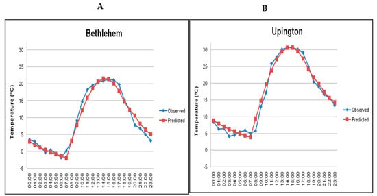
Figure 3. Temperature curves for Station (A) and Station (B) on 26 July 2006 derived from Sinusoidal model (TDM).

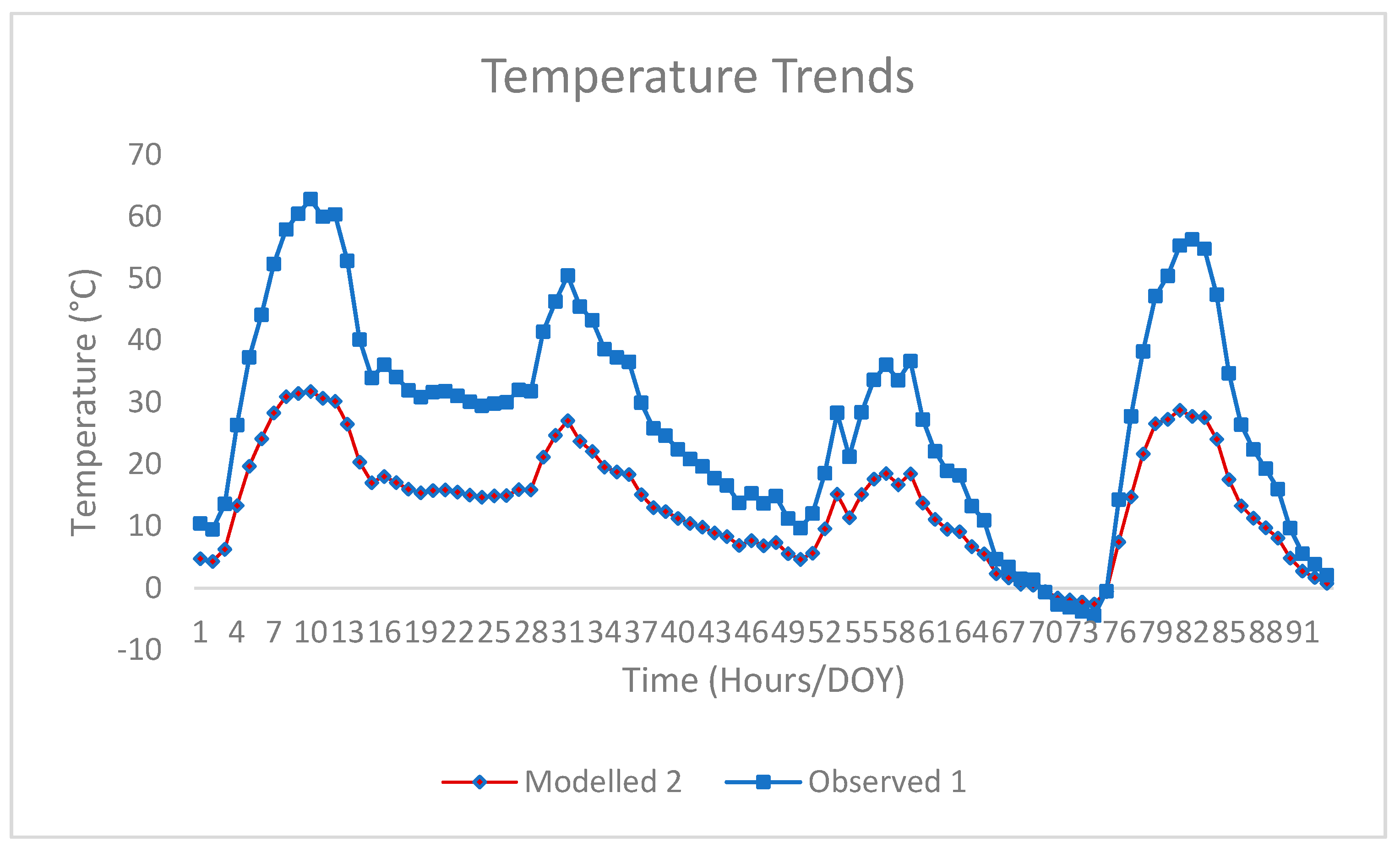
The trend or line graph of the short day’s data sets shows the underestimation of the actual measured data by the wave model algorithm (Figure 3). The modelled hourly temperatures from the wave model algorithm were off by more than 2 °C, and the algorithm managed to predict the night-to-early morning temperatures better than the evening ones. The pattern of the hourly data between the modelled and the observed are similar, even though there is underestimation. The same errors with the uncorrected models at other times of the day were observed in the study conducted by [39] with −1.4 °C, and also in a study conducted by [1], who also observed the least variation between estimated and observed hourly temperature when the minimum temperature was recorded, and the highest was observed during other times of the day. Further, Cesaraccio et al. [39] reported that the maximum temperature did not appear to affect the accuracy of the models employed to estimate hourly temperature from daily data.

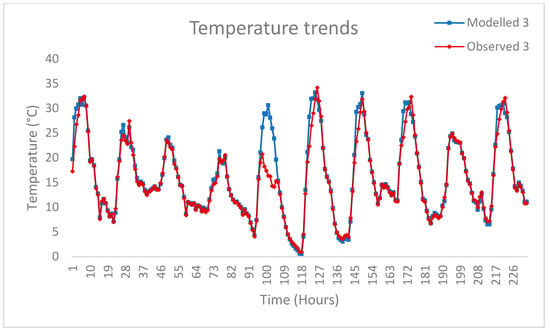
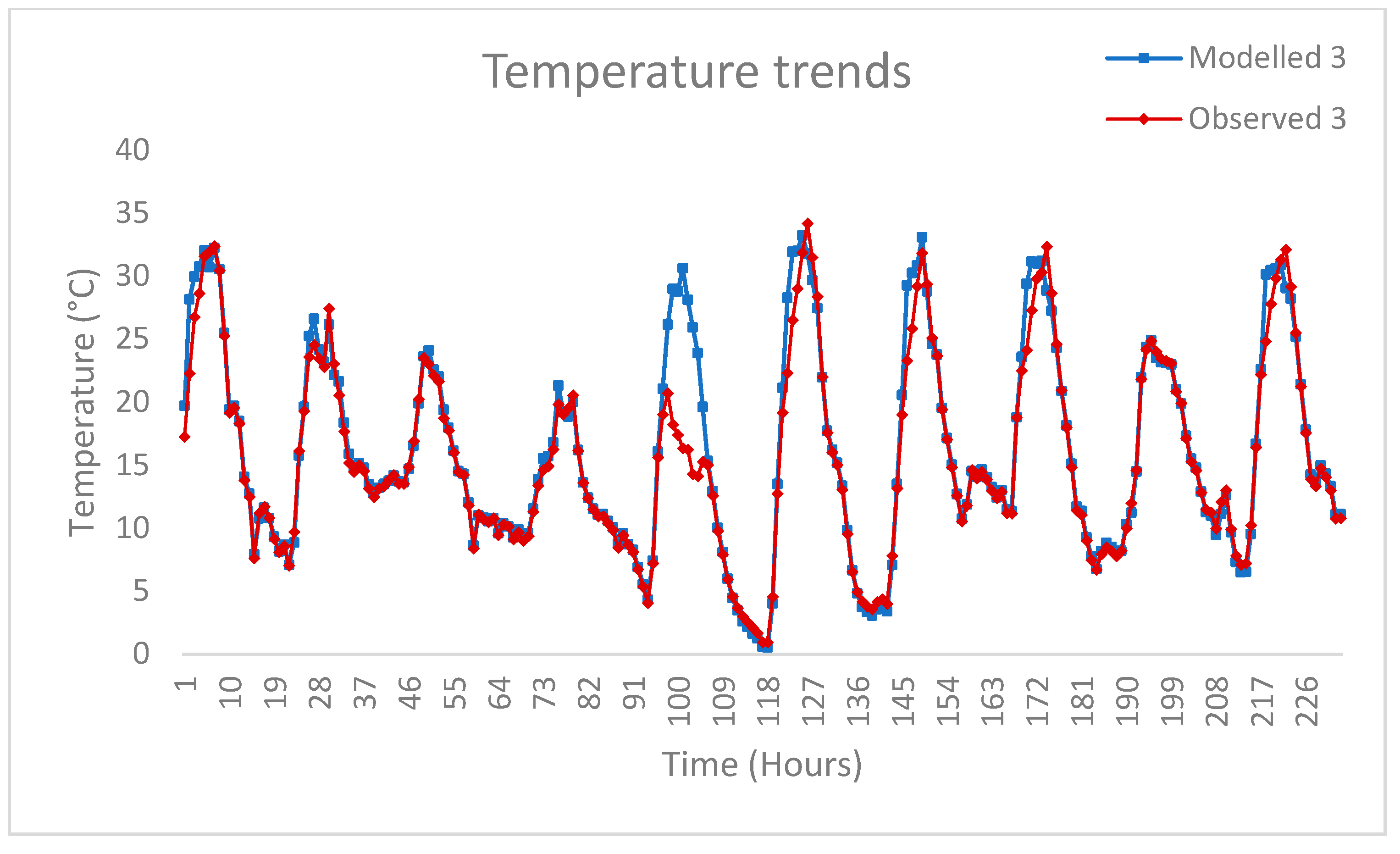
The underestimation of hourly temperatures by the wave model (Figure 4) could be attributed to the low diurnal variation in temperature that occurs during the winter season due to cloudy/overcast conditions for most of the day. Reicosky et al. [1] also found that predicted hourly temperature data from daily maximum and minimum temperatures fitted well during cloud-free days than cloudy days [15,37].

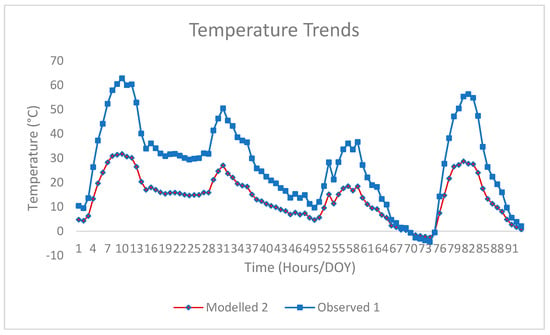
Figure 4. The trends of modelled and observed temperatures from the wave model algorithm using a few number of days.

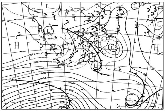
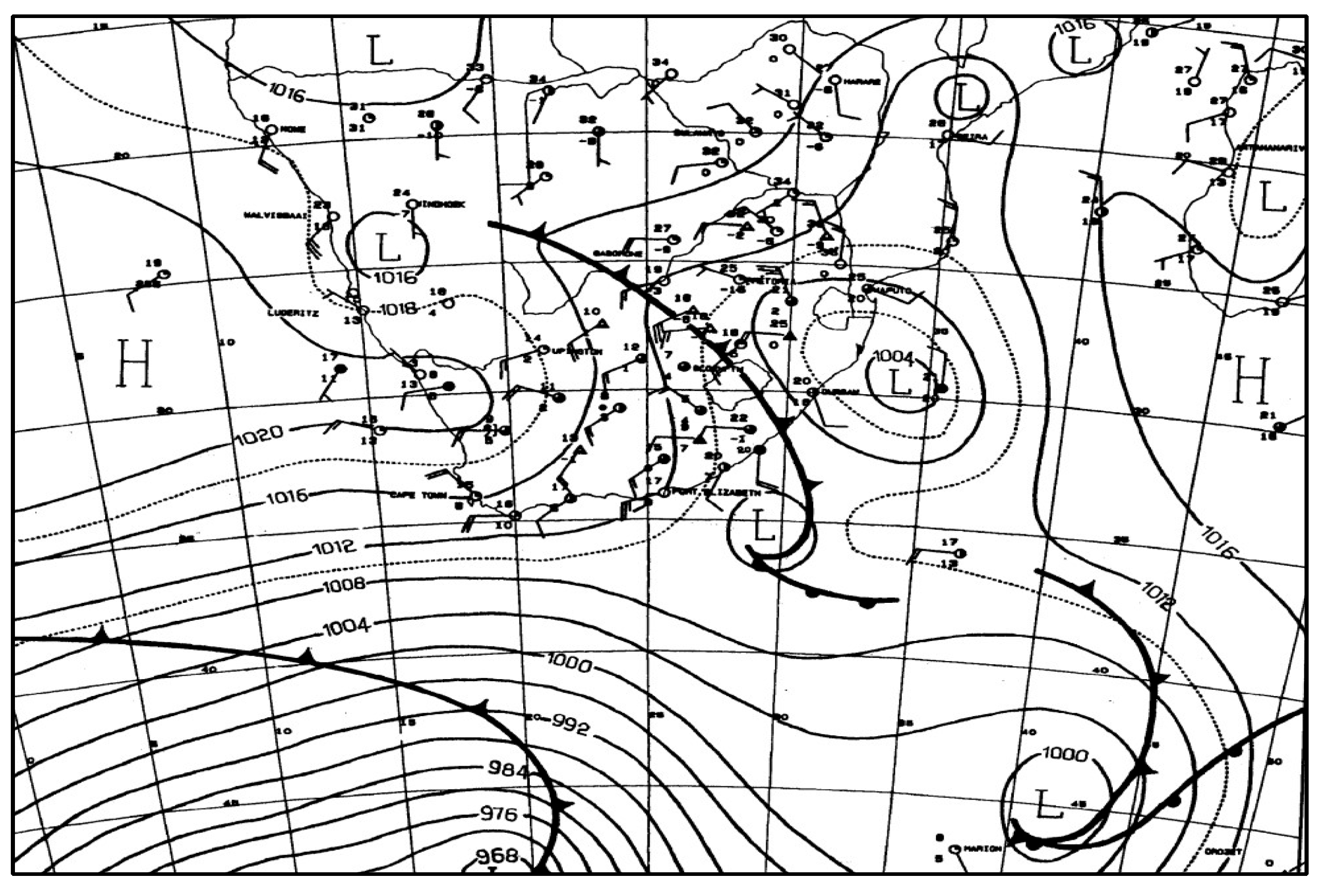
The synoptic chart (Figure 5) clearly shows the temperatures during the previous day and those of the current day. The difference between the temperatures of the area, which the cold front has also passed, is low compared to the areas which did not yet receive the cold front. The cold front’s trajectory showed its impact on the cloud cover, with a sudden drop in temperature and also changes in the direction of winds. The Sinusoidal model was unable to simulate the sudden changes in temperatures due to the passing of the cold front, which created a rapid decline in the temperatures recorded during the day (Figure 6). The same test was conducted on the data sets using the wave model and other different algorithms, but they all failed to simulate the sudden temperatures, based on the assumptions made for all the models. The input for all the models is just two variables, the minimum and the maximum temperatures, which makes it difficult to know what has happened during the course of the day.

Figure 5. Synoptic weather map of southern Africa, indicating a cold front over the eastern Free State at 14:00 on 27 August 1996 [17].

Figure 6. Temperature curve for station during the cold front passing over on 27 August 1996.

The long-term data or the use of more days, which tend to generate the average temperature trends, also failed to simulate or show the sudden changes in temperatures from the Wave model, which was used in the machine learning testing of the data and the model capability. It is clearly depicted in Figure 7 that the model could not simulate the sudden changes in temperatures, as it is not a forecasting model but a model based on observed data for certain times of the day.

Figure 7. The diurnal trend of the modelled data using the wave model embedded with parabolic methods.

The model data from the wave model also failed to simulate the diurnal trend when there was a sudden change in weather activity. The algorithm did not detect the timing of the cold front in the observed data. There is a difference between weather forecasting and prediction models, as those have different inputs compared to the modelling of the historical diurnal trend. When comparing the data simulated from the same model in Figure 5 and the data in Figure 7, it is clear that when adding more days to the data sets, the underestimation of the observed data or the overestimation disappears. The fewer the number of days, the clearer the flaws in the model tend to be, whereas large data sets tend to hide the flaws by averaging the trends. The long term, the average data set shows the consistency of the modelled temperatures vs. the observed temperatures is also due to the driest season of the year, during which mostly clear days and nights are observed.

4. Conclusions

Simple mathematical models based on trigonometric functions were developed to generate high-temporal-resolution temperature data for two locations in South Africa. The models used daily minimum and maximum temperatures, together with the day of the year, as input variables. Evaluation of the Temperature Derivation Model (TDM) using statistical performance indicators, including mean absolute error (MAE), root mean square error (RMSE), coefficient of determination (R²), and mean error (ME), demonstrated good agreement between the derived and measured hourly temperature data.

The results indicate that the derived hourly temperature values can serve as valuable inputs for crop growth models and other applications requiring high-resolution temperature information at specific locations. Among the models evaluated, the Sinusoidal method, which incorporates daily maximum, minimum, and average temperatures, reproduced hourly temperature patterns more accurately than algorithms based solely on daily maximum and minimum temperatures.

The timing assigned to daily temperature extremes was found to be critical for accurately reconstructing hourly temperatures. For all models, the most suitable times were 06:00 for the daily minimum temperature and 14:00 for the daily maximum temperature. The analysis further revealed that the optimal time for the daily minimum temperature corresponds closely to the hour before sunrise, while the timing of the daily maximum temperature aligns with recommendations provided by the World Meteorological Organization (WMO).

One important application of simulated hourly temperature data is within the deciduous fruit industry, including peach, sweet cherry, apple, and grapevine production systems. These industries rely on the calculation of chilling hours and chill units to monitor the accumulation of winter chilling and assess progress toward meeting crop-specific chilling requirements. The model performed particularly well under stable weather conditions. However, users should exercise caution when applying the TDM over short time periods, as abrupt temperature changes associated with weather disturbances, such as cold fronts, may reduce model accuracy.

The revised temperature-extreme timings are not exclusive to the Sinusoidal algorithm and can be adopted to improve traditional methods that rely only on daily maximum and minimum temperature observations. The algorithm is especially useful for generating future hourly temperature estimates from 7-day and 14-day weather forecasts, as well as from the outputs of global and regional climate models. This is particularly valuable because most climate prediction models provide daily maximum, minimum, and average temperatures rather than hourly temperature data.

Bias correction using linear regression was found to be highly effective in reducing model errors across all seasons and locations. The magnitude of errors in both uncorrected and bias-corrected models varied throughout the 24 h cycle, reflecting temporal differences in model performance. Comparative evaluation of four temperature estimation models across diverse agroecological regions of South Africa showed that the Wave model performed best during the summer season in hot sub-humid and semi-arid environments. In contrast, the Sinusoidal (TDM) model outperformed the other models during spring across most locations, ranging from hot per-humid to hot semi-arid climates.

The ability to generate accurate hourly temperature datasets from daily maximum and minimum temperature observations is particularly valuable where continuous hourly records are unavailable, incomplete, or interrupted. Such reconstructed datasets provide an important resource for agricultural, environmental, hydrological, and climate-related applications that require high-temporal-resolution temperature information.

References

- Reicosky, D.C.; Winkelman, L.J.; Baker, J.M.; Baker, D.G. Accuracy of hourly air temperatures calculated from daily minima and maxima. Agric. For. Meteorol. 1989, 46, 193–209. [Google Scholar] [CrossRef] [Scilit]
- Linvill, D.E. Calculating chilling hours and chill units from daily maximum and minimum temperature observations. HortScience 1990, 25, 14–16. [Google Scholar] [CrossRef] [Scilit]
- Bulut, H.; Buyukalaca, O.; Yilmaz, T. New models for simulating daily minimum, daily maximum and hourly outdoor temperatures. Proc. First Int. Exergy Energy Environ. Symp. 2003, 1, 499–504. [Google Scholar]
- Ephrath, J.E.; Goudriaan, J.; Marani, A. Modelling diurnal patterns of air temperature, radiation wind speed and relative humidity by equations from daily characteristics. Agric. Syst. 1996, 51, 377–393. [Google Scholar] [CrossRef] [Scilit]
- Richardson, E.A.; Seeley, S.D.; Walker, D.R. A model for estimating the completion of rest for ‘Red haven’ and ‘Elberta’ peach trees. HortScience 1974, 9, 331–332. [Google Scholar] [CrossRef] [Scilit]
- Knight, K.M.; Klein, S.A.; Duffie, J.A. A methodology for the synthesis of hourly weather data. Sol. Energy 1991, 46, 109–120. [Google Scholar] [CrossRef] [Scilit]
- Hoogenboom, G.; Huck, M.G.; Peterson, C.M. Root Growth Rate of Soybean as Affected by Drought Stress 1. Agron. J. 1987, 79, 607–614. [Google Scholar] [CrossRef] [Scilit]
- Yoshida, H. Modeling of weather data by time series analysis for air-conditioning load calculations. ASHRAE Trans. 1992, 98, 328–345. [Google Scholar]
- Alaruri, S.D.; Amer, M.F. Empirical regression models for weather data measured in Kuwait during the years 1985, 1986, and 1987. Sol. Energy 1993, 50, 229–233. [Google Scholar] [CrossRef] [Scilit]
- Sezai, I.; Taşdemiroǧlu, E. Evaluation of the meteorological data in Northern Cyprus. Energy Convers. Manag. 1995, 36, 953–961. [Google Scholar] [CrossRef] [Scilit]
- Sfetsos, A.; Coonick, A.H. Univariate and multivariate forecasting of hourly solar radiation with artificial intelligence techniques. Sol. Energy 2000, 68, 169–178. [Google Scholar] [CrossRef] [Scilit]
- Cesaraccio, C.; Spano, D.; Snyder, R.L.; Duce, P. Chilling and forcing model to predict bud-burst of crop and forest species. Agric. For. Meteorol. 2004, 126, 1–13. [Google Scholar] [CrossRef] [Scilit]
- Mellit, A.; Benghanem, M.; Kalogirou, S.A. An adaptive wavelet-network model for forecasting daily total solar-radiation. App. Energy 2006, 83, 705–722. [Google Scholar] [CrossRef] [Scilit]
- Shtiliyanova, A.; Bellocchi, G.; Borras, D.; Eza, U.; Martin, R.; Carrère, P. Kriging-based approach to predict missing air temperature data. Comput. Electron. Agric. 2017, 142, 440–449. [Google Scholar] [CrossRef] [Scilit]
- Elbeltagi, A.; Vishwakarma, D.K.; Katipoğlu, O.M.; Sushanth, K.; Heddam, S.; Singh, B.P.; Shukla, A.; Gautam, V.K.; Pande, C.B.; Hussain, S.; et al. Air temperature estimation and modeling using data driven techniques based on best subset regression model in Egypt. Sci. Rep. 2025, 15, 20200. [Google Scholar] [PubMed]
- Moore, J.L.; Remais, J.V. Developmental models for estimating ecological responses to environmental variability: Structural, parametric, and experimental issues. Acta Biotheor. 2014, 62, 69–90. [Google Scholar] [CrossRef] [Scilit]
- SAWS. Climate Data Supplied by South African Weather Service Climate Data Bank; SAWS: Pretoria, South Africa, 2013. [Google Scholar]
- Morrill, J.C.; Bales, R.C.; Conklin, M.H. Estimating stream temperature from air temperature: Implications for future water quality. J. Environ. Eng. 2005, 131, 139–146. [Google Scholar] [CrossRef] [Scilit]
- McCann, I.R. A Soil Temperature Model for Predicting the Overwinering Emergence of Heliothis Zea and Heliothis Virescens. Ph.D. Thesis, Texas A & M University, College Station, TX, USA, 1985. [Google Scholar]
- Liu, C.; Hofstra, N.; Leemans, R. Preparing suitable climate scenario data to assess impacts on local food safety. Food Res. Int. 2015, 68, 31–40. [Google Scholar] [CrossRef] [Scilit]
- Buzzi, A.; Foschini, L. Mesoscale meteorological features associated with heavy precipitation in the southern Alpine region. Meteorol. Atmos. Physics. 2000, 72, 131–146. [Google Scholar] [CrossRef] [Scilit]
- Ren, G.; Zhou, Y.; Chu, Z.; Zhou, J.; Zhang, A.; Guo, J.; Liu, X. Urbanization effects on observed surface air temperature trends in North China. J. Clim. 2008, 21, 1333–1348. [Google Scholar] [CrossRef] [Scilit]
- Parton, W.J.; Logan, J.A. A model for diurnal variation in soil and air temperature. Agric. For. Meteorol. 1981, 23, 205–216. [Google Scholar] [CrossRef] [Scilit]
- Eckersten, H. Simulated willow growth and transpiration: The effect of high and low resolution weather data. Agric. For. Meteorol. 1986, 38, 289–306. [Google Scholar] [CrossRef] [Scilit]
- Sargent, R.G. Verification and validation of simulation models. J. Simul. 2013, 7, 12–24. [Google Scholar] [CrossRef] [Scilit]
- Chow, D.H.C.; Levermore, G.J. New algorithm for generating hourly temperature values using daily maximum, minimum and average values from climate models. Build. Serv. Eng. Res. Technol. 2007, 28, 237–248. [Google Scholar] [CrossRef] [Scilit]
- Schlesinger, S. Terminology for model credibility. Simulation 1979, 32, 103–104. [Google Scholar] [CrossRef] [Scilit]
- Banks, J.; Carson, J.S.; Barry, L.N.; David, M.N. Discrete-Event System Simulation, 5th ed.; Pearson Education: Upper Saddle River, NY, USA, 2010. [Google Scholar]
- Chai, T.; Draxler, R.R. Root mean square error (RMSE) or mean absolute error (MAE)?—Arguments against avoiding RMSE in the literature. Geo. Model Dev. 2014, 7, 1247–1250. [Google Scholar] [CrossRef] [Scilit]
- Hamilton, J.D. Time Series Analysis; Princeton University Press: Princeton, NJ, USA, 1994. [Google Scholar]
- Hyndman, R.J.; Koehler, A.B. Another look at measures of forecast accuracy. Int. J. For. 2006, 22, 679–688. [Google Scholar] [CrossRef] [Scilit]
- Vemuri, S.; Hoveida, B.; Mohebbi, S. Short term load forecasting based on weather load models. Power Syst. Power Plant Control 1987, 20, 315–320. [Google Scholar] [CrossRef] [Scilit]
- Draper, N.R.; Smith, H. Serial correlation in the residuals and the Durbin–Watson test. In Applied Regression Analysis, 3rd ed.; John Wiley & Sons: Hoboken, NJ, USA, 2014; pp. 179–203. [Google Scholar]
- Everitt, B.; Skrondal, A. The Cambridge Dictionary of Statistics, 106; Cambridge University Press: Cambridge, UK, 2002. [Google Scholar]
- Arnold, J.G.; Moriasi, D.N.; Gassman, P.W.; Abbaspour, K.C.; White, M.J.; Srinivasan, R.; Santhi, C.; Harmel, R.D.; Van Griensven, A.; Van Liew, M.W.; et al. SWAT: Model use calibration validation. Trans. ASABE 2012, 55, 1491–1508. [Google Scholar] [CrossRef] [Scilit]
- Mohseni, O.; Stefan, H.G.; Erickson, T.R. A nonlinear regression model for weekly stream temperatures. Water Resour. Res. 1998, 34, 2685–2692. [Google Scholar] [CrossRef] [Scilit]
- Rodríguez, A.; Pérez-López, D.; Sánchez, E.; Centeno, A.; Gómara, I.; Dosio, A.; Ruiz-Ramos, M. Chilling accumulation in fruit trees in Spain under climate change. Nat. Hazards Earth Syst. Sci. 2019, 19, 1087–1103. [Google Scholar] [CrossRef] [Scilit]
- Luedeling, E.; Brown, P.H. A global analysis of the comparability of winter chill models for fruit and nut trees. Int. J. Biometeorol. 2011, 55, 411–421. [Google Scholar] [CrossRef] [Scilit] [PubMed]
- Cesaraccio, C.; Spano, D.; Duce, P.; Snyder, R.L. An improved model for determining degree-day values from daily temperature data. Int. J. Biometeorol. 2001, 45, 161–169. [Google Scholar] [CrossRef] [Scilit] [PubMed]
Disclaimer/Publisher’s Note: The statements, opinions and data contained in all publications are solely those of the individual author(s) and contributor(s) and not of MDPI and/or the editor(s). MDPI and/or the editor(s) disclaim responsibility for any injury to people or property resulting from any ideas, methods, instructions or products referred to in the content. |
© 2026 by the authors. Licensee MDPI, Basel, Switzerland. This article is an open access article distributed under the terms and conditions of the Creative Commons Attribution (CC BY) license.