


Abstract
In this study, we present a machine-learning approach—a land use random forest (LURF) model—to produce daily PM10 concentration maps at a 1 km resolution across the Campania region for the year 2022. The model combines daily measurements from 13 ARPA Campania monitoring stations with a wide set of spatial and atmospheric information. The predictors include population, land cover, road network, ERA5 meteorological data, satellite aerosol observations from MODIS, output from the CHIMERE chemistry transport model, and a flag identifying days affected by Saharan dust transport. The model is trained and validated using a station-based cross-validation scheme that accounts for spatial correlation between sites. Under this scheme, the LURF reproduces observed concentrations with substantially smaller errors than the raw CHIMERE output (RMSE of 11.0 vs. 23.6 g m−3). CHIMERE concentrations and ERA5 meteorology emerge as the most informative predictors, while the dust flag specifically improves the representation of episodic high-PM10 events. The resulting 1-km maps reveal clear urban–rural contrasts. They identify pollution hotspots in the Naples metropolitan area and along major motorways that are not visible in coarser model outputs. Probabilistic exceedance maps further show that meeting the future 2030 EU limit value of 20 g m−3 will be challenging across much of the metropolitan area. Overall, the proposed framework provides a low-cost, practical tool for high-resolution PM10 exposure assessment, supporting epidemiological studies, environmental justice analyses, and air quality management in regions with complex terrain and limited monitoring coverage.
1. Introduction
Particulate matter remains one of the most consequential air pollutants for public health across European and global contexts [1,2]. Chronic exposure to elevated PM10 concentrations is linked to a broad spectrum of adverse outcomes. These include cardiovascular and respiratory disease, premature mortality, and impaired agricultural productivity. The associated burdens fall disproportionately on residents of densely built city centres and other high-exposure microenvironments [1,2,3]. To contextualise the scale of the problem, the WHO Air Quality Guidelines set a PM10 annual mean guideline of 15 g m−3, while the current EU limit value stands at 40 g m−3. Annual mean concentrations in southern Italian urban areas regularly range between 25 and 45 g m−3, substantially exceeding the WHO guideline and approaching the EU limit [2,4]. Reliable, spatially resolved concentration estimates are therefore a prerequisite for epidemiological surveillance, health impact assessment, and implementation of the revised EU Air Quality Directive. The directive progressively tightens limit values towards World Health Organization guideline levels and demands more granular exposure information [2,5]. The core challenge is that regulatory monitoring networks, although providing high-quality measurements at a high temporal resolution, sample only a handful of locations per urban area. This sparse spatial footprint is insufficient to characterise the steep intra-urban gradients that develop downwind of traffic corridors, junctions, ports, or industrial zones, which are precisely the environments where human exposure is highest [6,7].
Land use regression (LUR) modelling was originally conceived to bridge the gap between discrete observations and spatially continuous concentration fields [8]. The approach links pollutant measurements at monitoring sites with geospatial covariates such as population density, land cover classes, road proximity, and meteorological context. These relationships are then projected across a fine-resolution grid. Over the past two decades, LUR methods have been widely adopted in multi-city European studies, most notably within the ESCAPE project [9,10,11], for mapping PM10, PM2.5, black carbon, and NO2 levels at spatial resolutions suitable for cohort-based health analyses [8,12]. Building on these foundations, more recent developments have integrated satellite-derived aerosol optical depth (AOD) products and chemistry transport model (CTM) output into the LUR predictor space. This integration improves coverage in regions with sparse ground monitoring and better constrains background aerosol fields [13,14].
The random forest extension of LUR, hereafter referred to as land use random forest (LURF), can accommodate nonlinear interactions and higher-order dependencies among predictors that classical linear LUR cannot capture. In this framework, ensembles of regression trees are trained on high-dimensional spatial covariate vectors and pollutant observations. The resulting model is then used to generate gridded concentration fields at resolutions much finer than the underlying monitoring network. LURF and related ensemble tree methods have been progressively adopted for mapping NO2 and particulate matter across European settings [12,15,16,17,18]. They offer improved predictive performance and robustness relative to traditional linear formulations, particularly under the small sample conditions typical of regulatory networks. In the Naples metropolitan area, for example, Chianese and Riccio [19] demonstrated the utility of the LURF approach for long-term NO2 exposure assessment by combining citizen science passive samplers with the ARPA Campania reference network. They achieved annual mean predictions with an uncertainty compatible with European Commission recommendations [5]. The present work builds on this methodological foundation and extends it to PM10 at the full regional scale of Campania.
Mapping PM10 poses particular challenges because this pollutant is a chemically and physically heterogeneous mixture. Road traffic emissions, brake and tyre wear, carbonaceous combustion products, marine sea salt, crustal material, and secondary inorganic aerosols each exhibit distinct spatial footprints and contrasting seasonal dynamics. Source apportionment and emission factor studies in Campania indicate that road traffic dominates PM in the Naples urban core, with maritime contributions more relevant at coastal sites, and show that even the inorganic ion fraction (nitrate, sulphate, and ammonium) retains spatial patterns linked to traffic intensity at the road segment scale [7]. Collectively, these findings motivate the adoption of a modelling architecture capable of resolving multi-source spatial heterogeneity; this is precisely the role that can be effectively addressed by an LURF ensemble. Among the episodic sources that can dominate daily PM10 in the Mediterranean basin, the long-range transport of Saharan mineral dust is particularly relevant. Such events can elevate ground-level concentrations by several tens of g m−3 within hours. They affect regulatory exceedance statistics and mask the local emission signal that the LURF approach is designed to resolve [20,21]. Explicitly flagging dust-affected days via the binary indicator IdDust allows the random forest to learn separate concentration–predictor relationships for dusty and non-dusty regimes, thereby reducing systematic underestimation on episodic high-PM10 days.
The LURF framework adopted here can be viewed as the spatial counterpart of machine learning models previously applied to air quality time series in southern Italy [22,23]. Rather than relying on temporal windows of past concentrations, it exploits the multivariate spatial structure embedded in land use-, road network-, meteorological-, satellite-, and CTM-derived predictors. The inclusion of meteorological data enriches the predictor space with information on boundary-layer dynamics, advection regimes, and moisture profiles. These factors influence PM10 dilution and transport across time scales ranging from hours to seasons [4,19].
The novelty of this study lies in the explicit integration of high-resolution CTM output, satellite-derived aerosol indicators, and ERA5 reanalysis within a unified random forest framework. This integration is combined with a spatially explicit validation strategy and the derivation of probabilistic exposure metrics at the regional scale. The hybrid use of CTM output is conceptually aligned with earlier European efforts that integrated CTM and satellite information into land use models for large-scale PM and NO2 mapping [13,14]. It is also aligned with the growing body of work combining meteorological data, satellite AOD, and machine learning for exposure estimation [4,24].
The primary research goals of this study are (1) to develop and validate an LURF model for spatially continuous daily PM10 mapping at a 1-km resolution across the Campania region; (2) to assess the added predictive value of embedding CTM output, satellite AOD, and ERA5 meteorology within the LURF predictor space; (3) to quantify the contribution of Saharan dust classification to model performance; and (4) to generate regulation-relevant annual exposure maps including probabilistic exceedance products for both the current EU limit and the forthcoming 2030 standard. From a practical standpoint, the resulting high-resolution maps can directly support epidemiological cohort studies, health impact assessments, and environmental justice analyses in the Campania region.
This paper is organised as follows. Section 2 describes the study area, monitoring data, and spatial predictor datasets, including the CTM configuration. Section 3 details the LURF architecture, predictor extraction, and cross-validation scheme. The results are presented in Section 4, which covers model performance, predictor importance, regional PM10 patterns, and a comparison with CHIMERE. Section 5 discusses the findings in the context of the LUR and LURF literature and highlights innovative aspects of the LURF–CHIMERE framework. It also explores implications for exposure and health impact assessment, together with limitations and future perspectives. Our conclusions are summarised in Section 6.
2. Study Area and Data
2.1. Study Domain
The Campania region (see Figure 1) lies along the eastern flank of the Tyrrhenian Sea in southern Italy. It covers approximately 13,600 km2 between the Apennine mountain chain to the northeast and the Gulf of Naples to the southwest. Its complex orography gives rise to a distinctive interplay between sea breeze circulation and orographic channelling, which strongly influences the accumulation and dispersion of primary and secondary aerosols. The Naples metropolitan area—home to roughly 3.1 million inhabitants and among the most densely urbanised territories in southern Europe—constitutes the dominant PM source region within this domain. Surrounding municipalities contribute additional industrial, agricultural, and maritime emissions. Together, these features make Campania an ideal, albeit demanding, test bed for spatially continuous PM exposure modelling.
Figure 1.
Map of European countries and Italian regions, with the Campania region outlined in bold black and highlighted in the upper-right inset.
2.2. Air Quality Monitoring Data
Observed daily mean PM10 concentrations were retrieved from the ARPA Campania regulatory monitoring network (see Figure 2) for the year 2022 [25]. The network comprises 42 stations spanning urban, suburban, traffic, industrial, and rural background typologies, classified in accordance with the European Air Quality Directive (2008/50/EC) [26]. However, only 13 stations provided quality-controlled PM10 records and were retained in this study. The remaining 29 stations either do not measure PM10 (monitoring NO2, O3, or PM2.5 only) or failed the quality control threshold of at least 75% valid daily observations over the 2022 reference period [5]. This threshold is the minimum data capture requirement prescribed by the EU Air Quality Directive for annual statistics. The 13 retained stations included 8 traffic, 3 industrial, and 2 background sites, providing a reasonable typological spread for training the LURF model across the range of exposure environments present in Campania. Table 1 summarises the name, type, coordinates, and data capture rate for each retained station. The spatial density of the retained network was approximately one station per 1046 km2. The eight traffic stations were mainly concentrated in the Naples metropolitan area while the three industrial stations lied in the northern Campania plain, and the two background stations occupied peri-urban locations north of Naples and the northern Campania plain. It is important to note that the limited number of monitoring stations () may have constrained the statistical representativeness of the training dataset, particularly in capturing the full range of spatial heterogeneity across rural and coastal environments. This limitation was partially mitigated by the inclusion of physically based predictors (e.g., CTM output and meteorological fields), which provided additional spatial structure beyond the monitoring network.
Figure 2.
Locations of ARPA Campania monitoring stations (black dots), with overlaid on the CORINE CLC map (level 1). The stations were unevenly distributed, with most concentrated in urban areas.
Table 1.
Summary of the 13 ARPA Campania PM10 monitoring stations retained in this study. Station types follow the EU Air Quality Directive (2008/50/EC) classification: T = traffic, I = industrial, and B = background. Data capture rate is the fraction of valid daily observations in 2022.
2.3. Spatial Predictors and ERA5 Reanalysis
Several categories of spatial predictors were assembled for each monitoring station within circular buffer radii of 20, 50, 100, 500, and 1000 m. Land cover information was drawn from the Corine Land Cover 2018 layer (CLC 2018) [27]. Individual classes were grouped into three broad categories: urban fabric, agriculture and natural vegetation, and water bodies. The built-up density and imperviousness fraction were extracted from the Copernicus High-Resolution Layers (HRLs) at a 10-m resolution [27]. Resident population counts were obtained from the Italian National Institute of Statistics (ISTAT) and disaggregated by census area. The road length and density by class were derived from the OpenStreetMap network (downloaded January 2026). Primary, secondary, and motorway classes were retained separately to reflect their contrasting emission profiles [7]. The distance to the nearest motorway centreline was also included as a geometric predictor.
Meteorological predictors—2-m air temperature (), dew point temperature (), surface pressure (), 10-m zonal () and meridional () wind components, and planetary boundary layer height (PBLH)—were derived from ERA5 global reanalysis at a 0.25° × 0.25° horizontal resolution (approximately 28 km over the Mediterranean).
A summary of all predictors, their sources, spatial resolutions, and buffer radii is provided in Table 2.
Table 2.
Summary of predictors used in the LURF model. Buffer radii apply to land use and road network variables; meteorological, AOD, and CTM predictors extracted as point values or spatially averaged over a 0.1° grid cell.
2.4. Satellite Aerosol Optical Depth
The columnar AOD at 550 nm was retrieved from the Collection 6.1 MCD19A2 product. This collection was sourced from NASA (National Aeronautics and Space Administration), Greenbelt, MD, USA, through the LAADS DAAC distribution system. Daily AOD values were quality-screened to retain only high-confidence retrievals. They were subsequently spatially averaged over a 0.1° × 0.1° grid centred on each monitoring station. The daily mean AOD, combining morning Terra and afternoon Aqua overpasses, was then computed for each station and used as a predictor variable. The dual-instrument configuration partially reduces diurnal sampling bias. It also provides a more representative estimate of daily aerosol loading, particularly over the frequently cloud-covered Campania coastline.
Missing AOD retrievals—arising from cloud cover or quality-screening rejection—were treated by exclusion. On days with no valid MAIAC pixel within the 0.1° aggregation box for a given station, the AOD and AOD/PBL predictors were set to NA (Not Available). The corresponding tree splits in the random forest then relied on the surrogate variable mechanism implemented in the ranger package [28], which selects the next best split predictor when the primary predictor is missing. This approach avoids imputation-induced bias while preserving the maximum number of training records.
In addition to the raw AOD, a derived variable was constructed by dividing the AOD by the planetary boundary-layer height (PBLH) obtained from ERA5, hereafter referred to as “AOD/PBL”. Specifically, AOD/PBL is the AOD value divided by PBLH, where AOD is dimensionless and PBLH is in metres, and thus the ratio’s unit is m−1. This variable provides a proxy for the near-surface aerosol concentration by accounting for vertical dilution processes within the boundary layer. While the AOD represents the total columnar aerosol load, its relationship with the surface PM10 depends strongly on the mixing depth of the atmosphere. For a given columnar aerosol burden, a deeper boundary layer implies greater vertical dispersion and thus lower surface concentrations. By contrast, shallow boundary-layer conditions favour pollutant accumulation near the ground. By dividing the AOD by the PBLH, the AOD/PBL indicator effectively incorporates this vertical mixing effect. It thereby enhances the physical interpretability of satellite-derived aerosol information and improves its relevance as a predictor of ground-level PM10 variability. Similar approaches have been widely adopted in the literature to improve the linkage between the columnar aerosol properties and ground-level concentrations, particularly under varying atmospheric stability conditions [29,30,31,32].
2.5. CHIMERE Chemical Transport Model Output
Gridded PM10 concentration fields were extracted from a CHIMERE [33,34,35] CTM simulation configured with a three-domain nested architecture and run for the full year of 2022. The European parent domain was discretised at a 25-km horizontal resolution, encompassing the entire continent. Nested Italian and Campania domains were run at 5-km and 1-km resolutions, respectively. The innermost domain covered the entire Campania region using a 390 × 382 grid cell configuration and fully encompassed the ARPA Campania monitoring network. All domains shared 14 terrain-following vertical layers starting at 20 m above ground level, with the layer thickness increasing with the altitude. Meteorological inputs were provided by the Weather Research and Forecasting (WRF) Model, driven by the NCEP initial and boundary conditions at a 0.25° × 0.25° resolution [36]. Anthropogenic and natural emissions for the European domain were derived from the CAMS-REG-ANT-v8.1 inventory [37], and emissions for the Italian and Campania nests were refined using high-resolution spatial proxies.
A multi-step downscaling procedure was implemented to redistribute emissions onto the target model grid. The downscaling procedure comprised two main stages: (1) sectoral mapping and (ii) spatial allocation. Emissions reported according to the nomenclature for reporting (NFR) classification were mapped onto Selected Nomenclature for Air Pollution (SNAP) sectors to enable sector-specific temporal and chemical profiles. Where a one-to-many correspondence existed between the NFR and SNAP categories, emissions were split using activity-based weighting factors derived from auxiliary datasets, such as fuel consumption, industrial statistics, or emission factor ratios. Spatial disaggregation was then performed using high-resolution reference datasets. These reference datasets are geospatial fields—derived from official statistics, land registries, or transport databases—that serve as spatial proxies for the activity intensity of a given emission sector within each model grid cell. Population density maps were used for residential combustion (SNAP 2); road network density were used for traffic emissions (SNAP 7); land use data were used for agricultural sources (SNAP 10); and industrial registries or point source databases were used for large combustion and industrial sectors (SNAP 3 and SNAP 4, respectively). Emissions were allocated to each grid cell according to
where is the emission assigned to grid cell i, is the total emission for a given sector and pollutant, is the value of the reference field (proxy) in cell i—for example, the population count for residential combustion or the road network density for traffic—and the denominator is the sum of the proxy values over all grid cells in the domain, ensuring that total emissions are conserved. The resulting emissions were formatted into NetCDF files compatible with the CHIMERE emission preprocessor (EMISURF).
The full modelling chain was run on a distributed HPC infrastructure using in-house tools [38,39,40,41].
2.6. Identification of Saharan Dust Days
Mineral dust transported from the Sahara Desert constitutes a recurrent and scientifically well-documented episodic perturbation to PM10 levels across the Mediterranean basin [20]. To represent this source explicitly in the LURF framework, a binary categorical variable IdDust was constructed for each day .
A day was labelled IdDust = 1 (dust-affected) only when all three of the following criteria were satisfied simultaneously:
- 1.
- Coarse fraction dominance: . The numerator represents the coarse particulate matter fraction, i.e., particles with an aerodynamic diameter between 2.5 and 10 m (“super-micron” or coarse-mode particles). A ratio above 0.5 means that more than half of the total PM10 mass is carried by these coarse, super-micron particles. Saharan mineral dust is predominantly in coarse mode, and thus this criterion selects days on which the aerosol composition is consistent with a crustal, dust-dominated regime rather than a fine mode-dominated anthropogenic regime (traffic, combustion, or secondary aerosol). This threshold is consistent with the aerosol-type discrimination approach developed for the Mediterranean by Barnaba and Gobbi [42], who showed that Saharan dust events are characterised by a marked shift towards coarse-mode aerosols relative to background continental or maritime conditions.
- 2.
- Elevated AOD: This indicates a daily mean AOD at 550 nm , derived from the MODIS Terra and Aqua MAIAC product described in Section 2.4. The threshold of 0.3 was not empirically chosen for this study; it was derived directly from the Mediterranean aerosol climatology of Barnaba and Gobbi [42] (Figure 1 in their work), who demonstrated that Saharan dust intrusions in the central Mediterranean are systematically associated with an MODIS AOD , while background continental and maritime aerosol conditions are characterised by an AOD under normal conditions. This climatological threshold thus provides a physically grounded and geographically appropriate criterion for dust episode detection over Campania.
- 3.
- PM10 exceedance: The third criterion requires the observed daily mean PM10 at station s to exceed the station-specific annual 75th percentile . The purpose of this criterion is straightforward; it restricts the IdDust flag to days with genuinely elevated concentrations. Even when the coarse fraction is high and the AOD is elevated, the PM10 level can remain within the normal range if the dust loading is moderate. By requiring that concentrations exceed the 75th percentile of the local annual distribution, we ensure that the flag identifies genuine concentration peaks, namely days when dust transport is not merely detectable but is actually driving the PM10 level above its typical seasonal background at that specific station.
Days satisfying the three criteria were further cross-checked against the operational ground-level dust surface concentration maps produced by the WMO Barcelona Dust Regional Center (BDRC; http://dust.aemet.es, accessed on 11 May 2026), operated jointly by the Agencia Estatal de Meteorología (AEMET) and the Barcelona Supercomputing Center (BSC) under WMO designation [21]. The BDRC provides daily dust forecasts and analysis maps at a resolution for the North African, Mediterranean, and European domain, and agreement between the derived IdDust flag and the BDRC dust surface concentration fields (daily maximum over Campania) was required to confirm each candidate dust episode. Of the candidate dust days identified by the three criteria, all were confirmed by the BDRC cross-check; no candidate days were rejected. In total, IdDust = 1 was assigned to 18 station days across the network during 2022, corresponding to six distinct calendar days with at least one affected station. These six events were distributed predominantly in spring (March–May), consistent with the known seasonal peak of Saharan dust transport to the central Mediterranean [20].
The PM2.5 data used in criterion (1) were available from a subset of the ARPA Campania network for the year 2022. At stations without co-located PM2.5 measurements, the coarse fraction criterion was evaluated using the network median PM2.5/PM10 ratio from stations where both species were measured on the same day, providing a conservative estimate of the coarse fraction. For stations and days where this imputation could not be applied with sufficient confidence (fewer than five co-measured station pairs on a given day), the IdDust flag was set to missing, and that record was excluded from training. In practice, imputation was required at 5 of the 13 stations (those without a co-located PM2.5 analyser) on all days with candidate dust episodes; the remaining 8 stations provided direct PM2.5 observations. Days with a missing IdDust flag (arising from imputation failures, i.e., fewer than five co-measured pairs) were excluded from the training set; this exclusion affected fewer than 2% of the total station day records.
3. Methods
3.1. Land Use Random Forest Framework
The LURF model follows the framework validated for long-term NO2 mapping in Naples [19] and extended from the spatiotemporal land use random forest approach developed for PM10 at a national scale in Italy by Stafoggia et al. [18]. It was adapted here for regional daily PM10 prediction. The modelling unit was the station–day pair , where s indexes the monitoring location and t is the calendar day. Each training record comprised a predictor vector and the corresponding observed daily mean PM10 concentration . The predictor vector included daily resolved ERA5 meteorological fields, CHIMERE PM10 levels, the MODIS AOD when available, the binary categorical variable IdDust, and time-invariant land use and road network descriptors. The resulting IdDust indicator was encoded as an integer binary variable ( non-dusty and dusty) and appended to the predictor vector .
3.2. Performance Metrics
Model performance was quantified using three standard metrics. The coefficient of determination is defined as follows:
where is the residual sum of squares and is the total variance of observations about their mean . A value of indicates a perfect prediction; indicates that the model is no better than a constant predictor equal to the observed mean; and indicates that the model performs worse than the observed mean, a situation that can arise when a deterministic model (such as a CTM) exhibits systematic biases large enough to produce residuals exceeding the natural variability of the observations. The root mean square error is , and the mean absolute error is . Both are expressed in g m−3 and equal zero for a perfect prediction. These metrics were computed by aggregating predictions and observations across all outer cross-validation folds (see Section 3.3).
3.3. Predictor Selection and Hyperparameter Optimisation
Model generalisability was assessed using a spatially structured cross-validation design defined at the station level and applied to the station day dataset. When station was assigned to the test fold, all associated daily observations were excluded from model fitting and used exclusively for validation, following a leave-location-out cross-validation (LLO-CV) scheme [43,44]. This approach is consistent with recent recommendations for spatially structured validation in machine learning models applied to environmental data [45,46].
The hyperparameters were optimised within a nested cross-validation framework. For each outer training set, an inner station-based cross-validation was used to perform a grid search over three hyperparameters: the number of predictor variables randomly sampled at each split (mtry), the minimum number of observations in the terminal nodes (min.node.size), and the number of trees in the ensemble (num.trees). The final model was then refitted on the full outer training set and evaluated on the corresponding held-out stations. Overall performance was quantified by aggregating the predictions across all outer folds. The grid search was conducted over the following sets: , and . These ranges were selected to cover the typical recommended values for random forest hyperparameters in regression settings [28,47]. Here, mtry was varied around the default of –5 (where p is the total number of predictors); min.node.size values of 3, 5, and 10 covered a range from flexible to conservative tree depth; and num.trees values of 500–1000 were generally sufficient for ensemble stabilisation. Table 3 summarises the grid and the most frequently selected values. Candidate configurations were ranked using the root mean square error (RMSE), and the optimal set was selected by minimising the RMSE. The most frequently selected hyperparameters across the outer folds were , , and .
Table 3.
Hyperparameter grid search ranges and most frequently selected values across outer LLO-CV folds.
3.4. Spatial Prediction and Uncertainty Mapping
Following hyperparameter selection, the model was refitted on the complete calibration dataset and applied to a 1-km prediction grid covering Campania. For each grid cell g and day t, the mean prediction across the decision trees provides the daily PM10 estimate . Annual statistics are then computed as temporal aggregates of the daily predictions at each grid cell. In particular, the annual mean PM10 concentration at grid cell g is defined as follows:
where T is the number of valid prediction days. Additional annual indicators (e.g., percentiles or exceedance counts) were derived consistently from the daily prediction time series .
The exceedance probability at each grid cell g is defined as the fraction of the individual tree predictions whose temporally aggregated annual mean exceeds a regulatory threshold :
where is the daily PM10 estimate of tree b at grid cell g on day t and is the indicator function. This formulation was applied to two regulatory thresholds: , corresponding to the current EU annual limit value under Directive 2008/50/EC, and , corresponding to the stricter limit value introduced by Directive (EU) 2024/2881 to be attained by 1 January 2030 [5]. This formulation propagates ensemble dispersion directly from the daily prediction scale to the annual regulatory indicator without assuming a parametric distribution for the tree-level predictions. It is, in this sense, a non-parametric analogue of probabilistic forecasting based on ensemble spread [48]. It should be noted, however, that daily predictions from the same tree share ERA5 and CHIMERE inputs across consecutive days. The inter-tree spread of the annual mean therefore primarily reflects structural uncertainty arising from the ensemble composition (bootstrap resampling and random feature selection), rather than the sampling uncertainty associated with temporal variability. The resulting exceedance probabilities should therefore be interpreted as a relative measure of prediction confidence across the grid cells, rather than as frequentist exceedance probabilities in a strict climatological sense.
3.5. Effective Spatial Resolution
While predictions were generated on a 1-km grid, the effective spatial resolution of the LURF output was constrained by the coarsest input predictors. ERA5 meteorological fields have a native resolution of ∼28 km; CHIMERE output was provided at 1 km but encoded physical smoothing at the grid cell scale; and the monitoring network density (one station per ∼1046 km2) further limited the spatial scales over which the statistical transfer function could be reliably estimated. In practice, the LURF output should be interpreted as a 1-km gridded field in which fine-scale gradients along road corridors and within the Naples metropolitan core are resolved by the road network and land use predictors, while background aerosol fields are modulated at the ERA5 and CTM scales. Claims of sub-kilometre precision are not made; the nominal 1-km grid spacing reflects the resolution of the output product and the finest spatial predictors (road network and imperviousness) and not the effective resolution of all input layers.
3.6. Ablation Experiment
To quantify the independent contribution of each major predictor group and address the concern that LURF may function primarily as a bias-corrected CTM rather than as an independent predictive framework, we performed an ablation experiment in which the LURF was retrained and re-evaluated under LLO-CV with three reduced predictor configurations: (1) No-CTM, with all predictors except CHIMERE PM10; (2) No-ERA5, with all predictors except ERA5 meteorological fields; and (3) No-AOD, with all predictors except the AOD and AOD/PBL. The performance metrics for each configuration are reported in Table 4 and discussed in Section 4.1.
Table 4.
Ablation experiment: LLO-CV performance of the full LURF model and three reduced predictor configurations. Removing CHIMERE produced the largest performance degradation, confirming its role as the dominant predictor; however, the No-CTM model still substantially outperformed the raw CHIMERE output, demonstrating that the LURF framework adds genuine predictive value beyond bias correction.
4. Results
4.1. Cross-Validation Performance and Error Structure
The predictive performance of the models was evaluated against the observed PM10 concentrations (from ARPA Campania’s daily mean in 2022) using standard error metrics as defined in Section 3.2 and a decomposition of the mean squared error (MSE) into systematic and random components.
The CTM output exhibited poor agreement with the observations, with , an RMSE of g m−3, and an MAE of g m−3 (see Figure 3). The negative value indicates that the raw CHIMERE output performed worse than a simple predictor equal to the observed annual mean. This is a direct consequence of the strong systematic underestimation of the peak concentrations and the large positive bias at the background sites, as illustrated by the shallow regression slope in Figure 3 (left panel). Decomposition of the MSE reveals that a substantial fraction of the error was systematic. This is evidenced by the shallow slope of the regression line and the strong underestimation of high PM10 concentrations. These results indicate that the CTM failed to reproduce both the magnitude and variability of the observed concentrations. The most likely causes are unresolved local emission sources and the spatial smoothing inherent to kilometre-scale grid discretisation.
Figure 3.
Observed versus predicted daily mean PM10 concentrations at ARPA Campania monitoring stations. The left panel shows the comparison with raw CHIMERE output (, RMSE g m−3, MAE g m−3), whereas the right panel reports the LLO-CV results for the LURF model (, RMSE g m−3, MAE g m−3). The dashed line denotes the 1:1 relationship, and the solid line indicates the least squares regression fit. Observations on dust days (IdDust = 1) are plotted as red-filled circles.
In contrast, the LURF model showed a marked improvement, with , an RMSE of g m−3, and an MAE of g m−3. The regression slope was closer to unity, indicating a substantial reduction in systematic bias. Although the predictive performance () represents a substantial improvement over the CTM baseline, a significant fraction of the variance remains unexplained. The most likely contributors are unresolved local emission sources, measurement representativeness errors, and the intrinsic stochasticity of particulate matter dynamics. The MSE decomposition suggests that the remaining error is predominantly random, reflecting residual variability not captured by the predictor set. Some dispersion persisted, particularly at higher concentration levels, indicating that extreme events remain only partially resolved.
To assess the specific performance on high-concentration events, we separately computed the error metrics for observations above 50 g m−3 (the EU daily limit value). For this subset ( station day records), the LURF achieved an RMSE of g m−3 and a mean bias of g m−3 (systematic underestimation), compared with an RMSE of g m−3 and a mean bias of g m−3 for the raw CHIMERE output on the same subset. Of these 47 high-concentration records, 31 (66%) coincided with IdDust = 1 days, confirming that Saharan dust transport was the dominant driver of extreme PM10 events in the dataset. At IdDust = 1 days alone, including the IdDust predictor reduced the mean bias from g m−3 (model without IdDust) to g m−3 (full LURF model), representing a 26% reduction in systematic underestimation during dust episodes.
The results of the ablation experiment (Table 4) confirm that CHIMERE was the most influential single predictor group; removing it degraded from 0.54 to 0.38 and increased the RMSE from 11.0 to 13.7 g m−3. Critically, however, the No-CTM configuration still achieved , substantially better than the raw CHIMERE output (), demonstrating that the LURF framework adds genuine predictive value beyond statistical bias correction of CTM output. Removing the ERA5 meteorological predictors produced a comparable but slightly smaller degradation (), while removing the satellite AOD variables had the smallest effect (). These results confirm that the LURF approach operates as a hybrid framework that fuses complementary information from multiple physical sources, rather than as a simple post-processor of CHIMERE output.
A systematic inspection of the scatter plot (Figure 3, right panel) reveals a noteworthy clustering of observations on IdDust days (red-filled circles, defined in Section 2.6) in the upper-right region of the diagram. These observations correspond to PM10 values well above 50 g m−3. On these days, LURF predictions tended to fall below the 1:1 line, indicating systematic underestimation that was larger in magnitude than the residuals observed for non-dusty days at comparable concentration levels. This bias is physically interpretable. During Saharan dust intrusions, the dominant PM10 source is long-range transported crustal aerosols. Such a source regime is morphologically and chemically distinct from the traffic, biomass combustion, and secondary aerosol signals that governed the non-dusty training population. The inclusion of the binary IdDust flag in the predictor vector partially mitigated this effect. It enabled the random forest approach to route tree splits into a dust-specific sub-space, thereby reducing the systematic underestimation relative to a model trained without any dust episode identifier. The residual bias visible in Figure 3 on IdDust days therefore represents the irreducible component that cannot be recovered from the available predictor set. This finding motivates the future replacement of the binary flag with a continuous dust surface concentration field (Section 5).
No marked over-prediction at the most polluted sites was evident. This differential bias is frequently observed in linear LUR applications but is largely suppressed in tree-based ensembles [14,49]. These performance figures are comparable to those reported in recent machine learning-based PM mapping studies that integrate satellite, meteorological, and land use predictors at regional and continental scales [15,16,17,18,50,51].
Residual diagnostics (Figure 4) revealed a near-Gaussian error distribution centred close to zero, with a mean bias of g m−3. This indicates the practical absence of systematic model bias. The distribution was, however, negatively skewed (skewness ), and a Shapiro–Wilk test formally rejected strict normality (). This departure from Gaussian behaviour was driven by a tail of large negative residuals at the highest observed concentrations (above ∼80 g m−3). Such residuals suggest a tendency to underestimate some extreme PM10 episodes, possibly linked to the limited number of training samples at such concentrations or to episodic transport events that were not fully captured by the daily mean CTM predictor. Inspection of the scatter diagram (Figure 3, right panel) further reveals that a disproportionate fraction of the largest negative residuals corresponded to observations on IdDust days (red-filled circles). This confirms that Saharan dust transport episodes were the primary driver of upper-tail underestimation.
Figure 4.
Residual diagnostics for LURF-predicted daily mean PM10 at ARPA Campania monitoring sites (skewness , Shapiro–Wilk p-value ). The dashed line represents the Gaussian fit to residuals. The histogram indicates an error distribution centred on zero with a slight negative skew driven by underestimation at the highest concentrations.
Heteroscedasticity was present in a mild form (see Figure 5). In particular, the spread of residuals became moderately wider and somewhat more asymmetric in the upper range of predictions, with a limited number of outliers. This pattern suggests that model uncertainty was not constant across the prediction domain and tended to increase with the PM10 levels. Such behaviour is consistent with the intrinsic variability of particulate matter, where higher concentrations are often associated with episodic events and local emission heterogeneity that are more difficult to capture with statistical models. The observed heteroscedasticity indicates that the model errors were dominated by random variability at low concentrations. By contrast, both the random and systematic components contributed at higher concentrations, leading to reduced predictive reliability in the upper tail of the distribution.
Figure 5.
Residuals (observed minus predicted daily mean PM10, g m−3) plotted against LURF-predicted values (g m−3) at ARPA Campania monitoring sites. The dashed horizontal line marks zero residual. Increasing spread at higher predicted concentrations reflects mild heteroscedasticity in the LURF error structure. Forecasts on dust days are plotted as red-filled circles.
Taken together, these diagnostics indicate that the predictor set captured the dominant emission patterns and meteorological modulation within Campania and that the remaining errors were compatible with typical regulatory PM10 measurement uncertainty and the representativeness error of fixed-site monitors in complex urban environments [3,8].
While the comparison against raw CTM output highlights the added value of the LURF framework, future work should also consider intermediate benchmarks (e.g., linear LUR or reduced-predictor models) to more explicitly quantify the contribution of each predictor group and to disentangle the respective roles of statistical learning and physical modelling.
4.2. Predictor Importance and Role of CHIMERE and ERA5
Figure 6 reports the relative importance of the main predictors entering the LURF model. CHIMERE PM10 fields, summarised at the monitoring locations, emerged as the single most influential predictor, accounting for ≈15.9 ± 1.4% of the total relative importance. The ERA5 mean sea-level pressure (mslp), 2-m air temperature (t2m), 10-m wind speed components (u10 and v10), 2-m dew point temperature (d2m), and planetary boundary-layer height (pbl) together contributed a further ≈40%. This indicates that large-scale and boundary-layer meteorological conditions exerted a strong control on the spatial variability of the daily mean PM10 level across the region. The AOD/PBL indicator () ranked as the second-most influential predictor, confirming that satellite aerosol products—once adjusted for vertical mixing—effectively captured background aerosol loading over both coastal and inland areas. In contrast, purely demographic or static land use descriptors such as the resident population showed comparatively low importance. This suggests that within the range of conditions sampled by the ARPA network, PM10 gradients were driven more by atmospheric dispersion and regional background than by population density alone.
Figure 6.
Relative importance of the top 10 predictors in the LURF model. Bars represent the mean relative importance (%) across outer-fold resampling, while error bars indicate the corresponding standard deviation, reflecting variability due to data partitioning. Importance was computed as the decrease in predictive performance (RMSE-based) when each predictor was randomly permuted. The AOD/PBL indicator was derived by dividing the MODIS AOD by the ERA5 boundary-layer height, accounting for vertical mixing effects.
However, the prominent role of CHIMERE as a predictor should be interpreted with caution. It reflects both the physical relevance of CHIMERE in representing regional background concentrations and its statistical correlation with observed PM10 levels. As demonstrated by the ablation experiment (Table 4), removing CHIMERE degraded model performance substantially but did not eliminate it; the LURF model without CTM still achieved , confirming that the framework is not reducible to a simple CTM bias correction. In this sense, the LURF model operates as a hybrid predictive framework in which CHIMERE provides the dominant regional background signal, ERA5 meteorology modulates boundary-layer dilution, and land use and road network predictors resolve fine-scale emission heterogeneity.
The binary categorical indicator IdDust (Section 2.6) appears among the secondary predictors in Figure 6, with a mean relative importance of approximately 3–5% (the precise value varied across the outer folds due to the limited number of dust-affected days in the 2022 dataset). Despite this modest overall weight, its inclusion produced a disproportionate improvement in the representation of the upper tail of the concentration distribution. On IdDust = 1 days, the LURF model is able to route tree splits towards a coarser aerosol dust-driven regime. This reduces the negative residuals that would otherwise arise from attempting to explain Saharan dust peaks with meteorological and traffic-based predictors alone. This behaviour is consistent with the known tendency of tree-based regressors to exploit categorical regime indicators for distributional partitioning [47]. It also aligns with the residual analysis of Section 4.1, where the largest negative residuals are concentrated precisely at the highest observed PM10 concentrations, events that predominantly correspond to dust episodes.
4.3. Regional PM10 Patterns at 1-km Resolution
The annual maps presented in this section were derived via temporal aggregation of daily LURF predictions, as described in Section 3.4, rather than being directly predicted as annual quantities.
4.3.1. LURF Annual Mean Map
The LURF-predicted annual mean PM10 (Figure 7) field revealed a pronounced urban–rural gradient over the Campania region. Peak concentrations—approaching or locally exceeding the EU annual limit value of 40 —were confined to the Naples metropolitan core, main motorway corridors, and select peri-urban industrial zones in the northern Campania plain. By contrast, elevated Apennine terrain, forested inland areas, and the southwestern coast remained around 30 . The spatial pattern was coherent with source apportionment evidence for the Campania domain, which attributed the high PM10 burden in the urban core primarily to road traffic, brake and tyre wear, and secondary inorganic aerosol [7]. Elevated concentrations also delineated the Port of Naples and the adjacent coastal infrastructure, where maritime emissions superimpose on road traffic signals in an area with sparse monitoring coverage.
Figure 7.
Spatial distribution of LURF-predicted annual mean PM10 concentrations across the Campania region at a 1-km resolution. Main roads are overlaid as thin lines.
4.3.2. CTM Annual Mean Map
The corresponding CHIMERE annual mean field (Figure 8) exhibited markedly different characteristics. The predicted concentrations spanned approximately 0–20 across the domain, falling substantially below the observed annual means at traffic and urban stations. The map shows a broad, spatially smooth hotspot centred on the Naples conurbation and its northern plain, reflecting the 1-km grid discretisation of the innermost CTM domain. However, sub-kilometre gradients along individual motorway corridors and port access roads are absent. Furthermore, concentrations in rural and mountainous areas were systematically overestimated relative to the LURF field. This pattern is consistent with the tendency of Eulerian transport models to spread emission plumes over coarser grid cells and underrepresent the steep near-road enhancements resolved by the LURF model [3].
Figure 8.
Spatial distribution of CTM-predicted annual mean PM10 concentrations across the Campania region at a 1-km resolution. Main roads are overlaid as thin lines. The colour scale is harmonised with Figure 7 for direct comparison.
4.3.3. Exceedance Probability Maps
Figure 9 shows the exceedance probability (Equation (2)) evaluated at two regulatory thresholds: (left panel), corresponding to the 2030 annual limit value under Directive (EU) 2024/2881 [5], and (right panel), corresponding to the current limit under Directive 2008/50/EC.
Figure 9.
Ensemble-based exceedance probability (Equation (2)) for the LURF-predicted annual mean PM10 level over the Campania region at a 1-km resolution. (left) Probability of exceeding the 2030 EU annual limit value of 20 (Directive (EU) 2024/2881). (right) Probability of exceeding the current EU annual limit value of 40 (Directive 2008/50/EC). Main roads are overlaid as thin lines.
For the current threshold, probabilities above 0.5 were confined to a compact zone encompassing the Naples metropolitan core (the Municipality of Naples, northern plain cluster, and western arc of the Campi Flegrei district), together with isolated hotspots along motorways. The majority of the Campania domain remained below 0.2, consistent with annual means in the 25–35 range.
For the stricter 2030 threshold , the spatial extent of high-probability cells expanded markedly. Probabilities above 0.5 covered not only the dense urban core but also a substantial fraction of the peri-urban plain extending northwards. This pattern reflects predicted annual means well above 20 over much of the metropolitan area. This result underscores the challenge that the Campania region—and southern Italian urban areas more broadly—will face in achieving compliance with the forthcoming 2030 standard. The finding is consistent with the gap documented by national-scale modelling studies [4].
The inter-tree standard deviation of the LURF ensemble (Figure 10) provided a spatially resolved measure of prediction uncertainty. Uncertainty was relatively low in the well-monitored urban core and along the main motorway axes, and it increased towards sparsely monitored mountainous and coastal areas, mirroring patterns reported in European-scale LURF and hybrid LUR/CTM studies [14,49].
Figure 10.
Standard deviation of LURF-predicted annual mean PM10 level (across 500 decision trees) at a 1-km resolution. Higher values indicate larger ensemble spread and, therefore, greater predictive uncertainty.
5. Discussion
5.1. Positioning and Innovative Aspects of the LURF–CHIMERE Framework
The Campania LURF model extends the growing family of land use-based machine learning frameworks for air quality exposure assessment. Compared with classical LUR studies developed within the ESCAPE project and subsequent multi-city efforts [8,9,11], the present work features four main distinguishing elements: (1) a random forest algorithm designed to handle high-dimensional, collinear predictor spaces; (2) the embedding of CTM-derived PM10 fields as a covariate, thereby fusing deterministic and statistical information; (3) the explicit classification of Saharan dust transport days via the binary indicator IdDust, constructed using the PM10/PM2.5 coarse fraction criterion and MODIS AOD thresholds and validated against WMO Barcelona Dust Regional Center operational products [21]; and (4) the application to a regional domain characterised by complex coastal and orographic meteorology and a heterogeneous mix of urban, industrial, and rural environments. Similar hybrid frameworks combining land use regression, satellite observations, and chemical transport modelling have been successfully applied across North America, Europe, and Asia [4,15,52,53,54], reinforcing the general applicability of the approach adopted here.
Recent reviews emphasise that machine learning extensions of LUR tend to outperform linear LUR in terms of predictive skill, particularly where monitoring is sparse and the spatial structure is complex [4,49]. The performance metrics reported in Section 4.1 are comparable to those of other European applications combining ERA5 reanalysis, satellite retrievals, and ground-based measurements, but the present framework differs in the explicit integration of a regional CTM field at a 1-km resolution. This positions the study close to the “hybrid” LUR/CTM/satellite models developed for NO2 and PM2.5 at continental scales [13,14], while pushing the spatial resolution down to 1000 m over a single, meteorologically complex region.
Several aspects of this study extend the current state of the art more specifically. The first distinguishing element is the hybrid use of a nested CTM as a predictor at a regional scale. Rather than relying on a generic continental CTM output, the present work integrates CHIMERE simulations from a dedicated three-domain nested configuration (25, 5, and 1 km) specifically tuned for Italy and Campania. The nested CHIMERE field provides a physically based background PM10 distribution that LURF refines to a 1000-m resolution, effectively implementing a CTM-informed statistical downscaling strategy. This hybrid architecture separates the problem into two complementary tasks: the CTM encodes regional-scale emission budgets and long-range transport dynamics, while the random forest algorithm learns the local transfer function that maps coarse grid cell concentrations onto the fine-scale emission heterogeneity captured by road network, land use, and boundary-layer predictors, a decomposition analogous to the “physical prior + statistical correction” paradigm advocated by de Hoogh et al. [14] and Fania et al. [4]. Closely related to this is the joint exploitation of ERA5, MODIS AOD, and CTM output within a single predictor space. The combination of ERA5 meteorological diagnostics, satellite-based AOD from the Terra and Aqua platforms, and CHIMERE concentration fields provides a rich, multi-source description of atmospheric processes across scales, fused with land use and traffic indicators. This degree of integration of reanalysis, satellite, and CTM information within a tree-based LURF framework has thus far received limited attention in the PM10 literature.
A further methodological contribution is the generation of probabilistic exceedance maps (Figure 9 defined formally in Equation (2)), an output layer absent in most comparable studies. By propagating ensemble uncertainty through to two regulatory indicators—the current EU limit of and the forthcoming 2030 limit of under Directive (EU) 2024/2881 [5]—the framework provides regulators and epidemiologists with spatially resolved risk products rather than point estimates. This output is conceptually analogous to probabilistic weather forecasting [48] and constitutes a significant step towards uncertainty-aware air quality assessment. Finally, the physical plausibility of the entire framework is underpinned by the rich body of local process knowledge available for the Campania domain. The region has been the subject of detailed emission factor and source apportionment studies [7]. Embedding these insights into the predictor design and interpretation illustrates how domain-specific, process-based understanding can guide and constrain the use of machine learning in air quality modelling.
5.2. Implications for Exposure and Health Impact Assessment
The exceedance-probability map (Figure 9) shows that probability values above 0.5 were spatially colocalised with the highest population density in the Naples metropolitan area. This implies that health burden estimates based on raw CTM output would systematically underestimate the fraction of the population exposed to concentrations above the EU’s limit value. This result has direct implications for health burden and environmental justice assessments, in line with recent work on high-resolution urban air pollution mapping and its use in environmental justice analyses [6,55]. The spatially resolved uncertainty estimates provided by the LURF ensemble further enable propagation of exposure uncertainty through to health impact calculations. This aspect is often treated only qualitatively in deterministic CTM studies [3,56].
Regarding the operational use of the model for real-time forecasting and early warning purposes, the LURF model as currently designed is a retrospective exposure mapping tool and not a real-time forecast system. All of its input predictors—ERA5 reanalysis, CHIMERE simulations, and MODIS AOD—are available only after the observation period has ended, with typical latencies ranging from hours (ERA5 near real time) to days (MODIS daily products). Consequently, the model in its present form cannot be used to issue same-day or next-day population warnings. However, the framework is architecturally compatible with a forecasting extension; ERA5 could be replaced by ECMWF operational forecasts (available up to 10 days in advance), and CHIMERE could be run in forecast mode, using forecast meteorology as the input. The MODIS AOD predictor could be approximated with Copernicus Atmosphere Monitoring Service (CAMS) aerosol optical depth forecasts. Such an extension would make the LURF framework operationally applicable for air quality warnings, and it is identified as a priority direction for future development.
5.3. Limitations, Critical Assessment, and Future Perspectives
Despite its strengths, the present framework has several limitations that merit explicit discussion. The first concerns network sparsity and spatial representativeness. The model was trained on 13 regulatory stations, the majority of which are located in or near the Naples metropolitan area. This uneven spatial coverage introduces a structural asymmetry; the LURF framework performed well in the well-observed urban domain but relied on extrapolation elsewhere. As correctly reflected by the ensemble uncertainty maps (Figure 10), predictive confidence decreased markedly over Apennine terrain and along the southern coastal fringe. The exceedance-probability map (Figure 9) should therefore be interpreted with caution in areas of high ensemble uncertainty, where low exceedance probabilities may partly reflect an insufficient training signal rather than genuinely clean air conditions. A more balanced station network—including rural background, coastal, and high-altitude sites—would be essential to consolidate the representativeness of regional exposure estimates. In terms of spatial representativeness, the 13 stations cover a region of approximately 13 600 km2, yielding an average density of one station per ∼1046 km2. By comparison, typical European ESCAPE studies operate at one station per ∼100–400 km2 within urban agglomerations [9]. The urban bias of the network (8 of 13 stations are classified as traffic) implies that the LURF transfer function is best constrained to urban traffic environments and that predictions for rural, coastal, and mountain sub-domains rely more heavily on physical extrapolation via CTM and ERA5 predictors. Despite this limitation, the small station count is not atypical for regional Italian studies and reflects the actual density of the ARPA Campania PM10 monitoring infrastructure. Any modelling approach operating in this context must accept the same constraint.
A second limitation concerns temporal scope. The present study was based on a single calendar year (2022) and produced an annual mean output only. While this is appropriate for regulatory compliance purposes, it precludes the characterisation of intra-annual variability that is ecologically and epidemiologically relevant. The Campania region is subject to marked seasonal contrasts. Summer sea breeze circulation promotes recirculation of polluted air masses in the Naples bay, whereas autumn and winter cold pool episodes lead to intense stagnation and biomass combustion episodes. A single annual mean map, whether LURF-based (Figure 7) or CTM-based (Figure 8), compresses this temporal complexity into a single spatial field, potentially masking seasonal exposure peaks of public health relevance. Extending the framework to monthly or seasonal maps—by incorporating time-stratified ERA5 and CHIMERE predictors—is therefore an important next step. A temporal leave-one-month-out cross-validation was not implemented in the present study because the training dataset was defined at the station day level, and the LLO-CV scheme already removed all temporal information from held-out stations; adding a temporal fold would further reduce the already small training set. Nonetheless, we acknowledge that seasonal validation is important for assessing model robustness across meteorological regimes, and we commit to implementing it in a multi-year extension of this work.
A third, methodologically more subtle limitation concerns the dual role of CHIMERE in this study. CHIMERE enters the LURF framework both as a predictor variable and as the deterministic benchmark against which LURF performance is assessed. This design is intentional. The LURF model was explicitly conceived as a statistical post-processor that learns to correct and downscale the CTM output using local observational and geospatial information in a manner conceptually analogous to model output statistics (MOS) approaches widely used in numerical weather prediction [48,57]. As a consequence, the performance gain of LURF over raw CHIMERE should be interpreted as the added value of data-driven downscaling and bias correction (Figure 7 versus Figure 8), rather than as evidence that the statistical model can operate independently of the CTM. Critically, this design also implies that systematic biases in CHIMERE will propagate into the LURF predictions. Examples include an underestimation of secondary inorganic aerosol formation during stagnation episodes or an inaccurate representation of maritime emission plumes in coastal grid cells. The degree of propagation depends on how consistently those biases manifest at the monitoring station locations included in the training set.
A further limitation concerns the potential bias of MODIS AOD retrievals over coastal and urban environments. The MAIAC algorithm is known to exhibit reduced accuracy over bright urban surfaces and near coastlines, where mixed land and sea pixels and aerosol–surface albedo interactions can introduce systematic retrieval errors [29,32]. Over the Naples coastal zone—precisely the area of highest exposure interest—this retrieval bias may introduce noise into the AOD and AOD/PBL predictors. The relatively modest contribution of these predictors in the ablation experiment (removing AOD reduced from 0.54 to 0.50) suggests that this bias, while non-negligible, did not dominate the overall model performance.
A further limitation specific to the IdDust categorical predictor concerns the availability and spatial representativeness of PM2.5 measurements within the ARPA Campania network. Because the PM2.5 level is not measured at all 13 stations retained in this study, the coarse fraction criterion required to assign IdDust = 1 must be partially imputed from the network median at the co-measuring stations on the same day (see Section 2.6). This imputation introduces an additional source of uncertainty for the stations and days where a PM2.5 level is absent. Moreover, the binary IdDust classification captures only the most intense dust episodes. It does not account for moderate or partially dust-contaminated days that fall below the combined threshold.
A final limitation concerns the interpretability of the random forest algorithm. While ensemble tree methods excel at capturing nonlinear associations, they do not provide the same level of parametric interpretability as classical regression models. Variable importance metrics (Figure 6) and partial dependence plots provide some insight. However, causal inference regarding individual predictors must remain grounded in process-based understanding and complementary modelling approaches [8,49]. In particular, the high importance attributed to CHIMERE (Figure 6) could partly reflect collinearity between the CTM field and other predictors (ERA5 and AOD/PBL) that are derived from the same meteorological forcing used to drive CHIMERE itself.
6. Conclusions
This study presented a hybrid land use random forest (LURF) model for spatially continuous PM10 exposure mapping across the Campania region at a 1-km resolution, trained on 2022 daily observations from 13 ARPA Campania regulatory stations and a high-dimensional predictor space comprising land use, road network, ERA5 meteorological, MODIS AOD, and CHIMERE CTM fields.
Under spatially aware leave-location-out cross-validation, the LURF model achieved a twofold reduction in error relative to the raw CHIMERE output (see Section 4.1). Residual diagnostics confirm the practical absence of systematic bias, while mild heteroscedasticity at the highest concentrations points to residual difficulties in representing episodic PM10 events. Predictor importance analysis identified the CHIMERE PM10 level as the single most influential covariate ( of total importance), followed by ERA5 pressure and boundary-layer fields (collectively ) and the AOD/PBL satellite composite. These results confirm that atmospheric dispersion and the regional background dominated PM10 variability over the region at the daily time scale. The binary categorical variable IdDust ranked among the secondary predictors and contributed to reducing systematic underestimation on episodic Saharan dust days, which accounted for some of the largest negative residuals observed under LLO-CV.
The 1-km annual mean maps resolved intra-urban gradients along motorway corridors and in the Naples metropolitan core that remained invisible at typical CTM grid spacings. Population-weighted exposure exceeded the simple area-averaged CTM estimate, with direct implications for health burden and environmental justice assessments. The probabilistic exceedance maps (Figure 9 and Equation (2)) further showed contrasting patterns at the two regulatory thresholds. Against the current EU limit of , probabilities above 0.5 were confined to the Naples metropolitan core and select motorway corridors. Against the forthcoming 2030 limit of under Directive (EU) 2024/2881 [5], high-probability cells expanded across the entire metropolitan area and peri-urban plain. This expansion highlights the scale of the compliance challenge that Campania—and comparable southern European urban regions—will face in the coming years.
Overall, the proposed framework demonstrates how the integration of physically based and data-driven approaches can enhance exposure assessment in data-sparse regions, while highlighting the need for careful interpretation of hybrid model outputs and continued investment in monitoring infrastructure.
Future developments should focus on a continuous dust-loading proxy—for example, the CHIMERE or CAMS dust surface concentration field—as a supplement or alternative to the binary flag. Such a proxy would allow the model to represent a continuum of dust influence rather than a hard classification. The extension of this framework to PM2.5 levels and the incorporation of time-varying ERA5 and CHIMERE predictors at a monthly resolution will enable seasonal exposure maps. Testing the transferability of the trained LURF framework to other Italian regions via domain adaptation strategies would further consolidate this approach as a versatile, low-cost complement to deterministic CTM modelling for regional air quality management.
Author Contributions
Conceptualisation, A.R. and E.C.; methodology, A.R. and E.C.; software, A.R.; validation, A.R. and E.C.; formal analysis, E.C.; investigation, E.C.; data curation, E.C.; writing—original draft preparation, E.C. and A.R.; writing—review and editing, A.R.; project administration, A.R. All authors have read and agreed to the published version of the manuscript.
Funding
This research received no external funding.
Institutional Review Board Statement
Not applicable.
Informed Consent Statement
Not applicable.
Data Availability Statement
Scripts used to implement the R-based workflow for training and validating the LURF model are publicly available at https://doi.org/10.5281/zenodo.19496301 under the GPL-3 license. ARPA Campania monitoring data are directly available (https://dati.arpacampania.it/dataset/dati-monitoraggio-qualita-aria, accessed on 11 May 2026). ERA5 reanalysis data are freely accessible from the Copernicus Climate Data Store (https://cds.climate.copernicus.eu, accessed on 11 May 2026). MODIS AOD products are distributed by NASA Earthdata (https://earthdata.nasa.gov, accessed on 11 May 2026). Corine Land Cover and Copernicus HRL data are available at https://land.copernicus.eu, accessed on 11 May 2026). Processed LURF outputs will be made available upon reasonable request to the corresponding author.
Acknowledgments
During the preparation of this manuscript, the authors used ChatGPT 5.5 for grammar checking and the preparation of figures and tables. The authors have reviewed and edited the output and take full responsibility for the content of this publication.
Conflicts of Interest
The authors declare no conflicts of interest.
References
- Cohen, A.J.; Brauer, M.; Burnett, R.; Anderson, H.R.; Frostad, J.; Estep, K.; Balakrishnan, K.; Brunekreef, B.; Dandona, L.; Dandona, R.; et al. Estimates and 25-year trends of the global burden of disease attributable to ambient air pollution: An analysis of data from the Global Burden of Disease Study 2015. Lancet 2017, 389, 1907–1918. [Google Scholar] [CrossRef] [Scilit]
- World Health Organization. WHO Global Air Quality Guidelines: Particulate Matter (PM2.5 and PM10), Ozone, Nitrogen Dioxide, Sulfur Dioxide and Carbon Monoxide; Technical Report; World Health Organization: Geneva, Switzerland, 2021. Available online: https://www.who.int/publications/i/item/9789240034228 (accessed on 1 April 2026).
- Solazzo, E.; Riccio, A.; Van Dingenen, R.; Valentini, L.; Galmarini, S. Evaluation and uncertainty estimation of the impact of air quality modelling on crop yields and premature deaths using a multi-model ensemble. Sci. Total Environ. 2018, 633, 1437–1452. [Google Scholar] [CrossRef] [Scilit] [PubMed]
- Fania, A.; Monaco, A.; Pantaleo, E.; Maggipinto, T.; Bellantuono, L.; Cilli, R.; Lacalamita, A.; La Rocca, M.; Tangaro, S.; Amoroso, N.; et al. Estimation of daily ground level air pollution in Italian municipalities with machine learning models using Sentinel-5P and ERA5 data. Remote Sens. 2024, 16, 1206. [Google Scholar] [CrossRef] [Scilit]
- European Commission. Directive (EU) 2024/2881 of the European Parliament and of the Council of 23 October 2024 on ambient air quality and cleaner air for Europe. Off. J. Eur. Union 2024. Available online: https://eur-lex.europa.eu/eli/dir/2024/2881/oj (accessed on 11 May 2026).
- Apte, J.S.; Manchanda, C. High-resolution urban air pollution mapping. Science 2024, 385, 380–385. [Google Scholar] [CrossRef] [Scilit]
- Riccio, A.; Chianese, E.; Tirimberio, G.; Prati, M. Emission factors of inorganic ions from road traffic: A case study from the city of Naples (Italy). Transp. Res. Part D Transp. Environ. 2017, 54, 239–249. [Google Scholar] [CrossRef] [Scilit]
- Hoek, G.; Beelen, R.; de Hoogh, K.; Vienneau, D.; Gulliver, J.; Fischer, P.; Briggs, D. A review of land-use regression models to assess spatial variation of outdoor air pollution. Atmos. Environ. 2008, 42, 7561–7578. [Google Scholar] [CrossRef] [Scilit]
- Eeftens, M.; Beelen, R.; de Hoogh, K.; Bellander, T.; Cesaroni, G.; Cirach, M.; Declercq, C.; Dëljus, E.; Dons, E.; Heinrich, J.; et al. Development of land use regression models for PM2.5, PM2.5 absorbance, PM10 and PMcoarse in 20 European study areas; results of the ESCAPE project. Environ. Sci. Technol. 2012, 46, 11195–11205. [Google Scholar] [CrossRef] [Scilit] [PubMed]
- Wang, M.; Beelen, R.; Basagaña, X.; Becker, T.; Cesaroni, G.; de Hoogh, K.; Dedele, A.; Declercq, C.; Dimakopoulou, K.; Eeftens, M.; et al. Evaluation of land use regression models for NO2 and particulate matter in 20 European study areas: The ESCAPE project. Environ. Sci. Technol. 2013, 47, 4357–4364. [Google Scholar] [CrossRef] [Scilit]
- Beelen, R.; Hoek, G.; Vienneau, D.; Eeftens, M.; Dimakopoulou, K.; Pedeli, X.; Tsai, M.Y.; Künzli, N.; Schikowski, T.; Marcon, A.; et al. Development of NO2 and NOx land use regression models for estimating air pollution exposure in 36 study areas in Europe–the ESCAPE project. Atmos. Environ. 2013, 72, 10–23. [Google Scholar] [CrossRef] [Scilit]
- Wolf, K.; Cyrys, J.; Harciníková, T.; Gu, J.; Kusch, T.; Hampel, R.; Schneider, A.; Peters, A. Land use regression modeling of ultrafine particles, ozone, nitrogen oxides and markers of particulate matter pollution in Augsburg, Germany. Sci. Total Environ. 2017, 579, 1531–1540. [Google Scholar] [CrossRef] [Scilit]
- Vienneau, D.; de Hoogh, K.; Beelen, R.; Fischer, P.; Hoek, G.; Briggs, D. Western European land use regression incorporating satellite- and ground-based measurements of NO2 and PM10. Environ. Sci. Technol. 2013, 47, 13555–13564. [Google Scholar] [CrossRef] [Scilit] [PubMed]
- de Hoogh, K.; Chen, J.; Gulliver, J.; Hoffmann, B.; Stafoggia, M.; Künzli, N.; Kloog, I.; Vineis, P.; Brunekreef, B.; Hoek, G.; et al. Development of West-European PM2.5 and NO2 land use regression models incorporating satellite-derived and chemical transport modelling data. Environ. Res. 2016, 151, 1–10. [Google Scholar] [CrossRef] [Scilit] [PubMed]
- Di, Q.; Amini, H.; Shi, L.; Kloog, I.; Silvern, R.; Kelly, J.; Sabath, M.B.; Choirat, C.; Koutrakis, P.; Lyapustin, A.; et al. An ensemble-based model of PM2.5 concentration across the contiguous United States with high spatiotemporal resolution. Environ. Int. 2019, 130, 104909. [Google Scholar] [CrossRef] [Scilit] [PubMed]
- Hu, X.; Waller, L.A.; Lyapustin, A.; Wang, Y.; Al-Hamdan, M.Z.; Crosson, W.L.; Estes, M.G., Jr.; Estes, S.M.; Quattrochi, D.A.; Puttaswamy, S.J.; et al. Estimating ground-level PM2.5 concentrations in the Southeastern United States using MAIAC AOD retrievals and a two-stage model. Remote Sens. Environ. 2014, 140, 220–232. [Google Scholar] [CrossRef] [Scilit]
- Chen, G.; Li, S.; Knibbs, L.D.; Hamm, N.A.; Cao, W.; Li, T.; Guo, J.; Ren, H.; Abramson, M.J.; Guo, Y. A machine learning method to estimate PM2.5 concentrations across China with remote sensing, meteorological and land use information. Sci. Total Environ. 2018, 636, 52–60. [Google Scholar] [CrossRef] [Scilit]
- Stafoggia, M.; Bellander, T.; Bucci, S.; Davoli, M.; de Hoogh, K.; De’ Donato, F.; Gariazzo, C.; Lyapustin, A.; Michelozzi, P.; Renzi, M.; et al. Estimation of daily PM10 and PM2.5 concentrations in Italy, 2013–2015, using a spatiotemporal land-use random-forest model. Environ. Int. 2019, 124, 170–179. [Google Scholar] [CrossRef] [Scilit]
- Chianese, E.; Riccio, A. Long-term variation in exposure to NO2 concentrations in the city of Naples, Italy: Results of a citizen science project. Sci. Total Environ. 2024, 931, 172799. [Google Scholar] [CrossRef] [Scilit]
- Vogel, F.; Putero, D.; Bonasoni, P.; Cristofanelli, P.; Zanatta, M.; Marinoni, A. Saharan dust transport event characterization in the Mediterranean atmosphere using 21 years of in-situ observations. Atmos. Chem. Phys. 2025, 25, 15453–15468. [Google Scholar] [CrossRef] [Scilit]
- WMO Barcelona Dust Regional Center. Operated by AEMET and BSC on behalf of WMO Daily Dust Products—Ground-Level Dust Concentration Maps. 2023. Available online: http://dust.aemet.es (accessed on 1 April 2026).
- Chianese, E.; Camastra, F.; Ciaramella, A.; Landi, T.; Staiano, A.; Riccio, A. Spatio-temporal learning in predicting ambient particulate matter concentration by multi-layer perceptron. Ecol. Inform. 2019, 49, 54–61. [Google Scholar] [CrossRef] [Scilit]
- Tateo, A.; Amoroso, N.; Bellantuono, L.; Monaco, A.; Pantaleo, E.; Maggipinto, T. Predicting Air Quality from Measured and Forecast Meteorological Data: A Case Study in Southern Italy. Atmosphere 2023, 14, 136. [Google Scholar] [CrossRef] [Scilit]
- Shtein, A.; Kloog, I.; Schwartz, J.; Silibello, C.; Michelozzi, P.; Gariazzo, C.; Viegi, G.; Forastiere, F.; Karnieli, A.; Just, A.C.; et al. Estimating daily PM2.5 and PM10 over Italy using an ensemble model. Environ. Sci. Technol. 2019, 54, 120–128. [Google Scholar] [CrossRef] [Scilit]
- Agenzia Regionale per la Protezione dell’Ambiente della Campania. Dati Monitoraggio Qualità dell’Aria, 2026. Data Set. Available online: https://dati.arpacampania.it/dataset/dati-monitoraggio-qualita-aria (accessed on 1 April 2026).
- European Parliament. Directive 2008/50/EC of the European Parliament and of the Council of 21 May 2008 on ambient air quality and cleaner air for Europe. Off. J. Eur. Union 2008. Available online: https://eur-lex.europa.eu/eli/dir/2008/50/2015-09-18 (accessed on 11 May 2026).
- Copernicus Land Monitoring Service. CORINE Land Cover, 2018. Available online: https://land.copernicus.eu/en/ (accessed on 1 April 2026).
- Wright, M.; Ziegler, A. ranger: A fast implementation of random forests for high dimensional data in C++ and R. J. Stat. Softw. 2017, 77, 1–17. [Google Scholar] [CrossRef] [Scilit]
- Hoff, R.M.; Christopher, S.A. Remote sensing of particulate pollution from space: Have we reached the promised land? J. Air Waste Manag. Assoc. 2009, 59, 645–675. [Google Scholar] [CrossRef] [Scilit]
- Gupta, P.; Christopher, S.A. Particulate matter air quality assessment using integrated surface, satellite, and meteorological products: Multiple regression approach. J. Geophys. Res. Atmos. 2009, 114, D14205. [Google Scholar] [CrossRef] [Scilit]
- Ma, Z.; Hu, X.; Sayer, A.M.; Levy, R.; Zhang, Q.; Xue, Y.; Tong, S.; Bi, J.; Huang, L.; Liu, Y. Satellite-based spatiotemporal trends in PM2.5 concentrations: China, 2004–2013. Environ. Health Perspect. 2015, 124, 184. [Google Scholar] [CrossRef] [Scilit]
- Li, T.; Shen, H.; Yuan, Q.; Zhang, X.; Zhang, L. Estimating ground-level PM2.5 by fusing satellite and station observations: A geo-intelligent deep learning approach. Geophys. Res. Lett. 2017, 44, 11–985. [Google Scholar] [CrossRef] [Scilit]
- Rouil, L.; Honoré, C.; Vautard, R.; Beekmann, M.; Bessagnet, B.; Malherbe, L.; Meleux, F.; Dufour, A.; Elichegaray, C.; Flaud, J.M.; et al. PREV’AIR: An operational forecasting and mapping system for air quality in Europe. Bull. Am. Meteorol. Soc. 2009, 90, 73–84. [Google Scholar] [CrossRef] [Scilit]
- Mailler, S.; Menut, L.; Khvorostyanov, D.; Valari, M.; Couvidat, F.; Siour, G.; Turquety, S.; Briant, R.; Tuccella, P.; Bessagnet, B.; et al. CHIMERE-2017: From urban to hemispheric chemistry-transport modeling. Geosci. Model Dev. 2017, 10, 2397–2423. [Google Scholar] [CrossRef] [Scilit]
- Mallet, V.; Menut, L.; Forêt, G.; Ung, A.; Achilleos, S.; Couvidat, F.; Quélo, D. The CHIMERE chemistry-transport model v2023r1. Geosci. Model Dev. 2024, 17, 5431–5457. [Google Scholar] [CrossRef] [Scilit]
- NOAA Physical Sciences Laboratory. NCEP/NCAR Reanalysis 1 Data Provided by the NOAA PSL, Boulder, Colorado, USA. Available online: https://psl.noaa.gov/data/gridded/reanalysis/ (accessed on 11 May 2026).
- Kuenen, J.; Dellaert, S.; Visschedijk, A.; Jalkanen, J.P.; Super, I.; Denier van der Gon, H. CAMS-REG-v4: A state-of-the-art high-resolution European emission inventory for air quality modelling. Earth Syst. Sci. Data 2022, 14, 491–515. [Google Scholar] [CrossRef] [Scilit]
- Giunta, G.; Montella, R.; Mariani, P.; Riccio, A. Modeling and computational issues for air/water quality problems: A grid computing approach. Nuovo C. Della Soc. Ital. Fis. C 2005, 28, 215–224. [Google Scholar] [CrossRef] [Scilit]
- Montella, R.; Giunta, G.; Riccio, A. Using grid computing based components in on demand environmental data delivery. In Proceedings of the Second Workshop on Use of P2P, GRID and Agents for the Development of Content Networks, Monterey, CA, USA, 26 June 2007; pp. 81–86. [Google Scholar]
- Riccio, A.; Ciaramella, A.; Giunta, G.; Galmarini, S.; Solazzo, E.; Potempski, S. On the systematic reduction of data complexity in multimodel atmospheric dispersion ensemble modeling. J. Geophys. Res. Atmos. 2012, 117, D05314. [Google Scholar] [CrossRef] [Scilit]
- Giunta, G.; Mariani, P.; Montella, R.; Riccio, A. pPOM: A nested, scalable, parallel and Fortran 90 implementation of the Princeton Ocean Model. Environ. Model. Softw. 2007, 22, 117–122. [Google Scholar] [CrossRef] [Scilit]
- Barnaba, F.; Gobbi, G.P. Aerosol seasonal variability over the Mediterranean region and relative impact of maritime, continental and Saharan dust particles over the basin from MODIS data in the year 2001. Atmos. Chem. Phys. 2004, 4, 2367–2391. [Google Scholar] [CrossRef] [Scilit]
- Roberts, D.R.; Bahn, V.; Ciuti, S.; Boyce, M.S.; Elith, J.; Guillera-Arroita, G.; Hauenstein, S.; Lahoz-Monfort, J.J.; Schröder, B.; Thuiller, W.; et al. Cross-validation strategies for data with temporal, spatial, hierarchical, or phylogenetic structure. Ecography 2017, 40, 913–929. [Google Scholar] [CrossRef] [Scilit]
- Ploton, P.; Mortier, F.; Réjou-Méchain, M.; Barbier, N.; Picard, N.; Rossi, V.; Dormann, C.; Cornu, G.; Viennois, G.; Bayol, N.; et al. Spatial validation reveals poor predictive performance of large-scale ecological mapping models. Nat. Commun. 2020, 11, 4540. [Google Scholar] [CrossRef] [Scilit]
- Meyer, H.; Reudenbach, C.; Hengl, T.; Katurji, M.; Nauss, T. Improving performance of spatio-temporal machine learning models using forward feature selection and target-oriented validation. Environ. Model. Softw. 2018, 101, 1–9. [Google Scholar] [CrossRef] [Scilit]
- Valavi, R.; Elith, J.; Lahoz-Monfort, J.J.; Guillera-Arroita, G. blockCV: An R package for generating spatially or environmentally separated folds for k-fold cross-validation of species distribution models. Methods Ecol. Evol. 2019, 10, 225–232. [Google Scholar] [CrossRef] [Scilit]
- Breiman, L. Random forests. Mach. Learn. 2001, 45, 5–32. [Google Scholar] [CrossRef] [Scilit]
- Wilks, D.S. Statistical Methods in the Atmospheric Sciences, 3rd ed.; Academic Press: Oxford, UK, 2011. [Google Scholar]
- Ma, X.; Zou, B.; Deng, J.; Gao, J.; Longley, I.; Xiao, S.; Guo, B.; Wu, Y.; Xu, T.; Xu, X.; et al. A comprehensive review of the development of land use regression approaches for modeling spatiotemporal variations of ambient air pollution: A perspective from 2011 to 2023. Environ. Int. 2024, 183, 108430. [Google Scholar] [CrossRef] [Scilit]
- Xue, T.; Zheng, Y.; Tong, D.; Zheng, B.; Li, X.; Zhu, T.; Zhang, Q. Spatiotemporal continuous estimates of PM2.5 concentrations in China, 2000–2016: A machine learning method with inputs from satellites, chemical transport model, and ground observations. Environ. Int. 2019, 123, 345–357. [Google Scholar] [CrossRef] [Scilit]
- Huang, K.; Xiao, Q.; Meng, X.; Geng, G.; Wang, Y.; Lyapustin, A.; Gu, D.; Liu, Y. Predicting monthly high-resolution PM2.5 concentrations with random forest model in the North China Plain. Environ. Pollut. 2018, 242, 675–683. [Google Scholar] [CrossRef] [Scilit]
- van Donkelaar, A.; Martin, R.V.; Brauer, M.; Kahn, R.; Levy, R.; Verduzco, C.; Villeneuve, P.J. Global estimates of fine particulate matter using a combined geophysical-statistical method with information from satellites, models, and monitors. Environ. Sci. Technol. 2015, 50, 3762–3772. [Google Scholar] [CrossRef] [Scilit]
- Kloog, I.; Chudnovsky, A.A.; Just, A.C.; Nordio, F.; Koutrakis, P.; Coull, B.A.; Lyapustin, A.; Wang, Y.; Schwartz, J. A new hybrid spatio-temporal model for estimating daily multi-year PM2.5 concentrations across northeastern USA. Atmos. Environ. 2014, 95, 581–590. [Google Scholar] [CrossRef] [Scilit]
- Just, A.C.; Wright, R.O.; Schwartz, J.; Coull, B.A.; Baccarelli, A.A.; Tellez-Rojo, M.M.; Moody, E.; Wang, Y.; Lyapustin, A.; Kloog, I. Using high-resolution satellite aerosol optical depth to estimate daily PM2.5 geographical distribution in Mexico City. Environ. Sci. Technol. 2015, 49, 8576–8584. [Google Scholar] [CrossRef] [Scilit] [PubMed]
- Southerland, V.A.; Brauer, M.; Mohegh, A.; Hammer, M.S.; Van Donkelaar, A.; Martin, R.V.; Apte, J.S.; Anenberg, S.C. Global urban temporal trends in fine particulate matter (PM2.5) and attributable health burdens: Estimates from global datasets. Lancet Planet. Health 2022, 6, e139–e146. [Google Scholar] [CrossRef] [Scilit] [PubMed]
- Solazzo, E.; Riccio, A.; Kioutsioukis, I.; Galmarini, S. Pauci ex tanto numero: Reduce redundancy in multi-model ensembles. Atmos. Chem. Phys. 2013, 13, 8315–8333. [Google Scholar] [CrossRef] [Scilit]
- Glahn, H.R.; Lowry, D.A. The use of model output statistics (MOS) in objective weather forecasting. J. Appl. Meteorol. Climatol. 1972, 11, 1203–1211. [Google Scholar] [CrossRef] [Scilit]
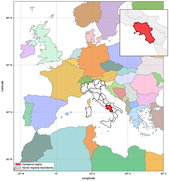
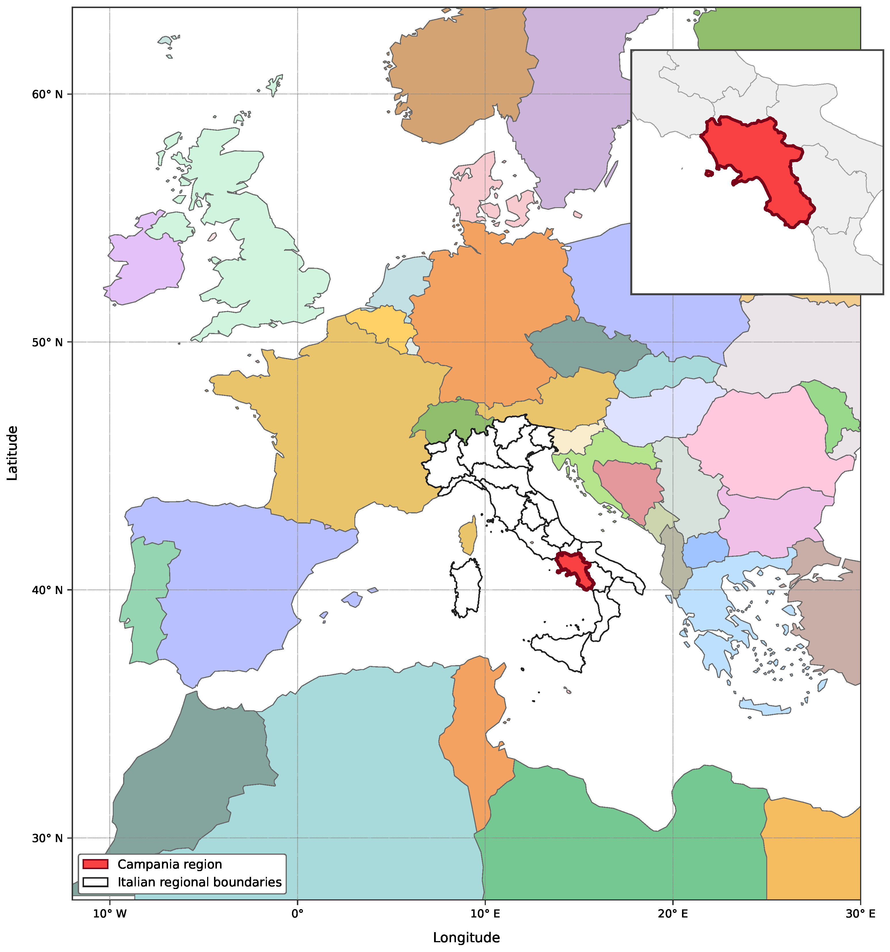
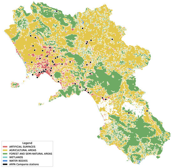
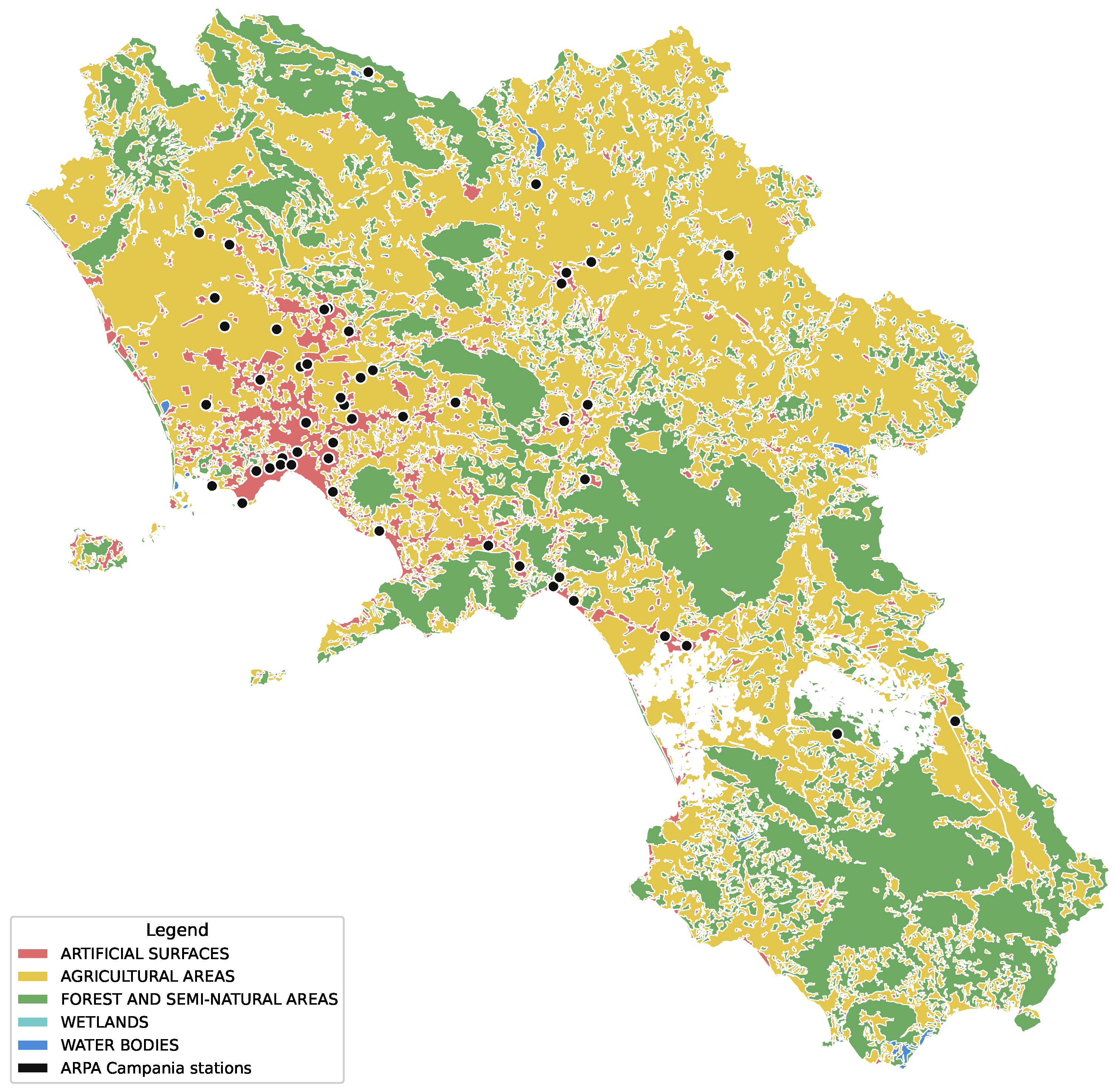
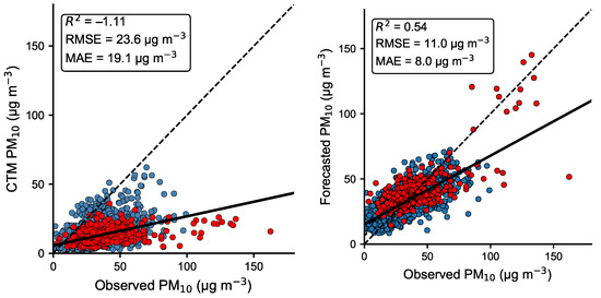
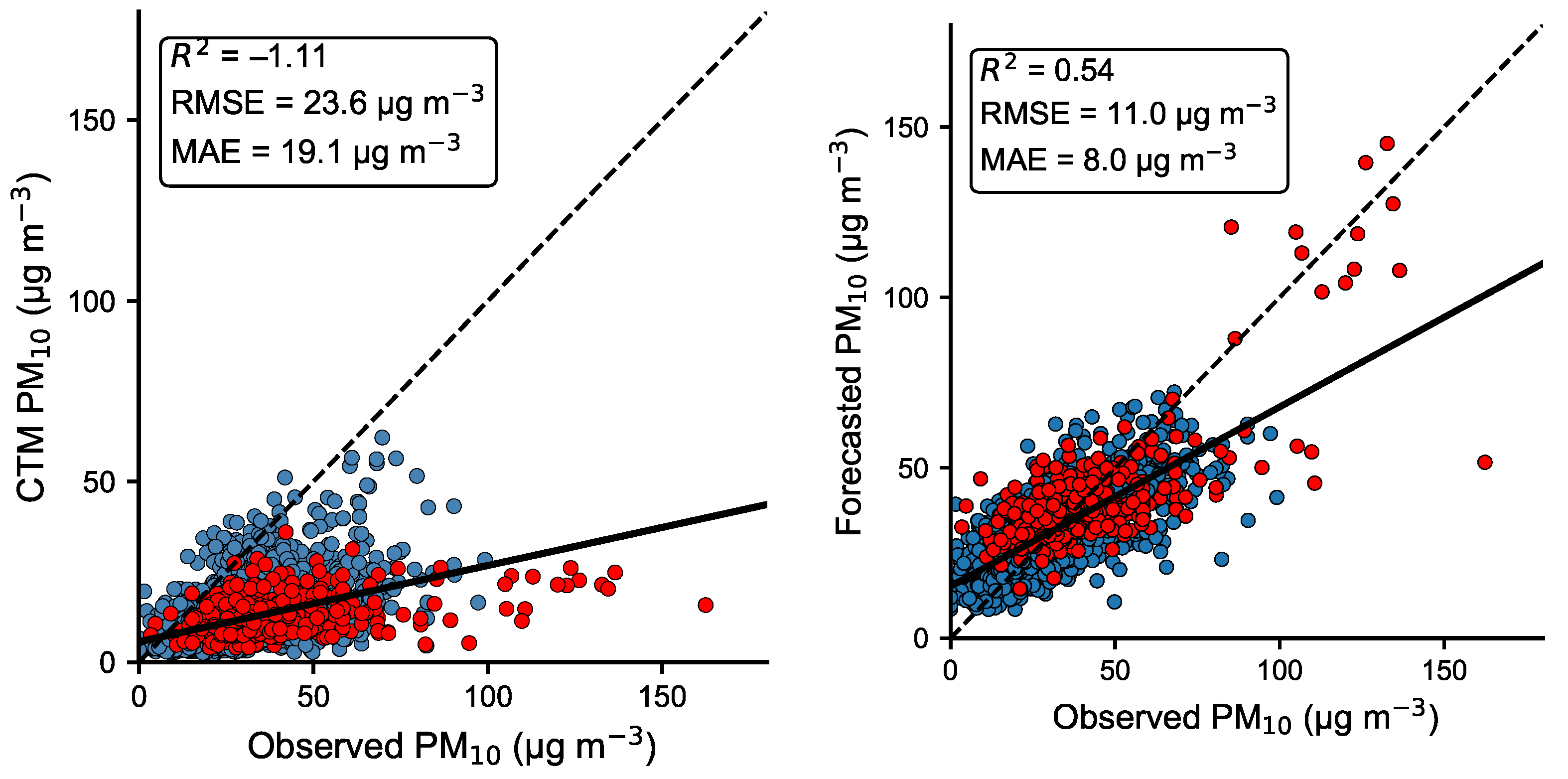
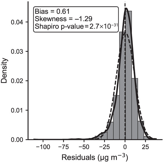
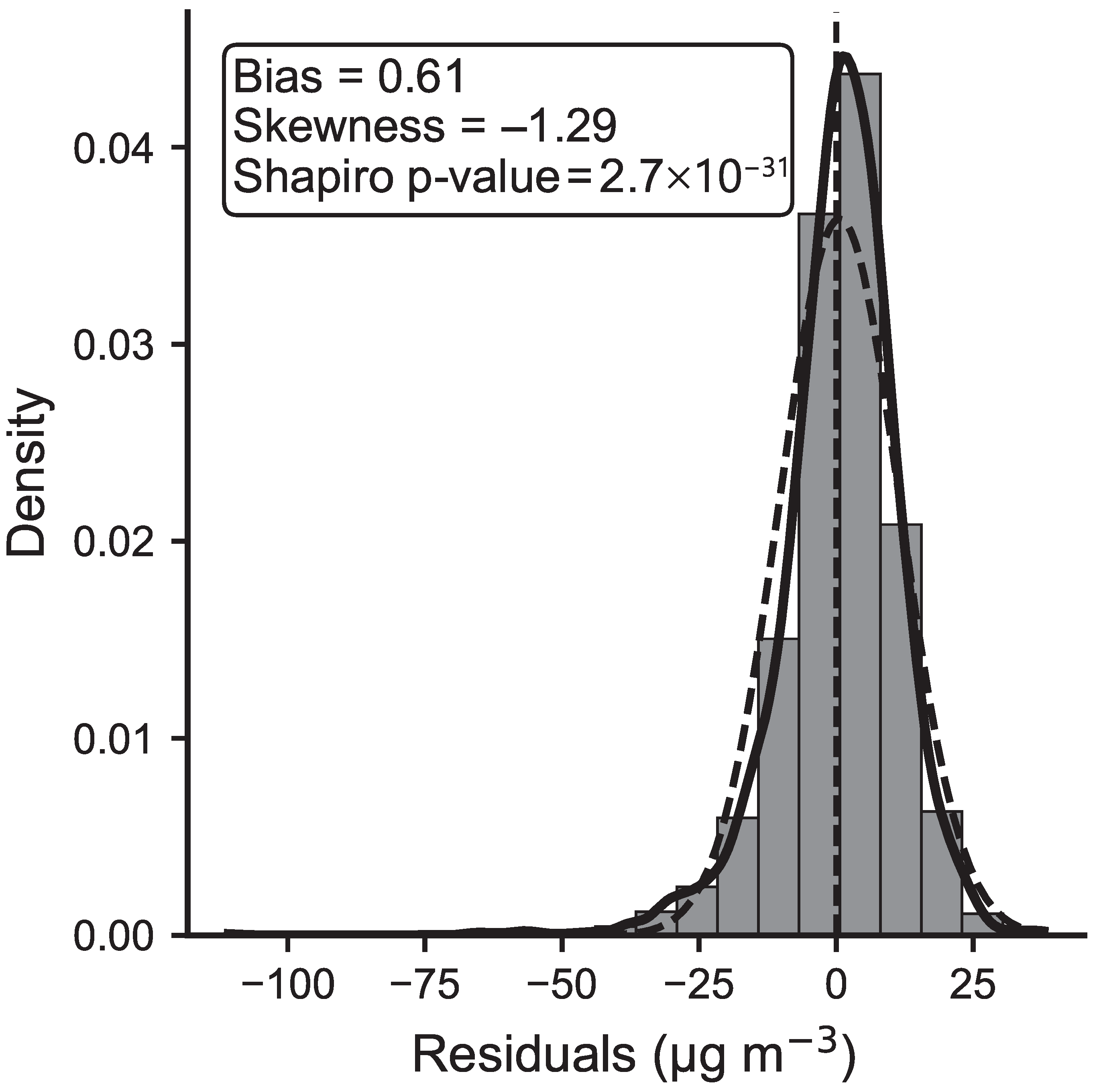
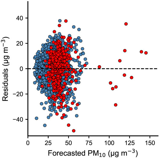
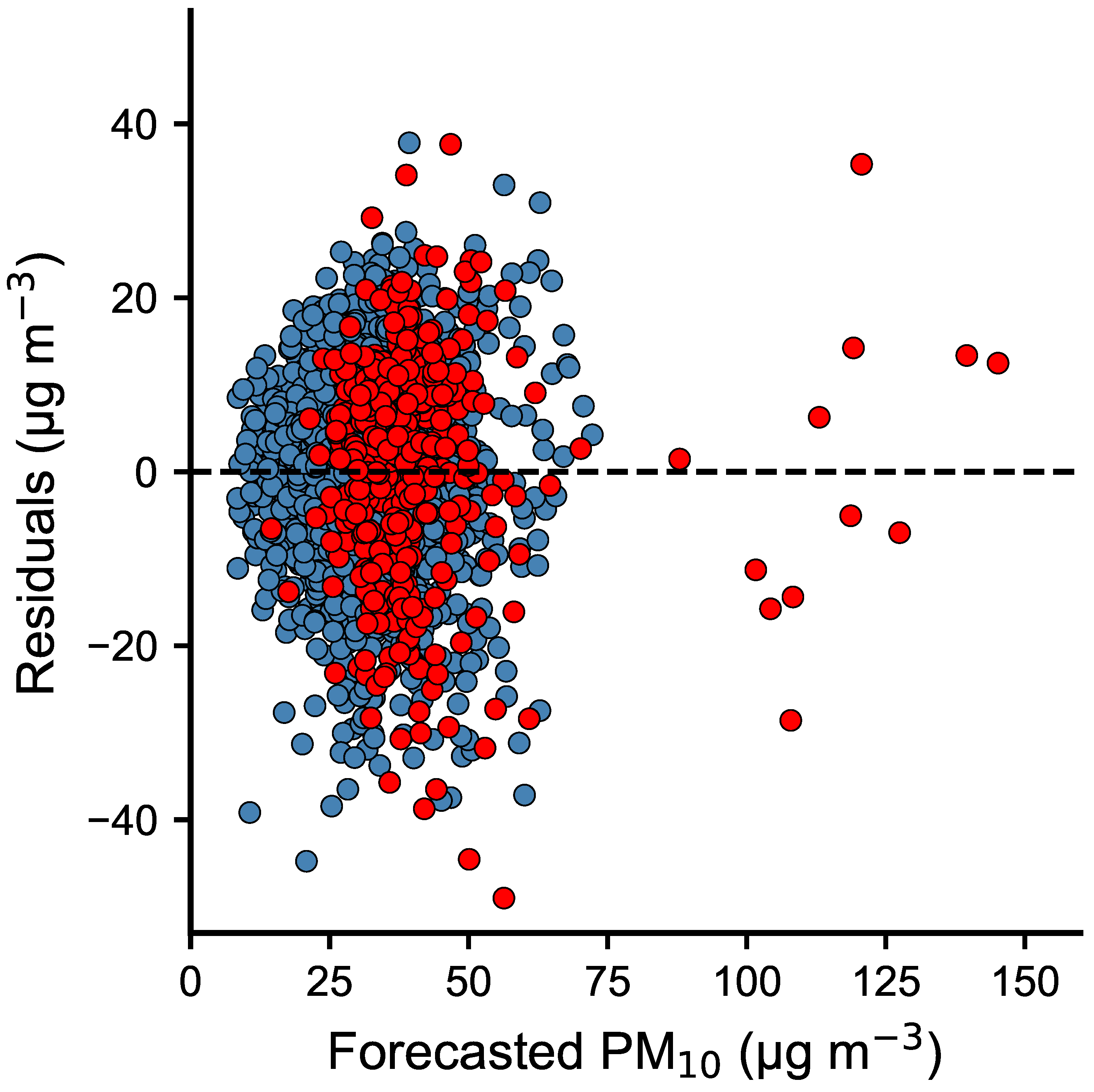
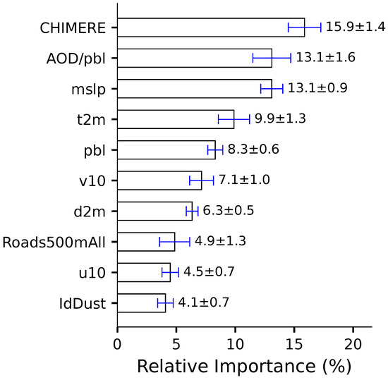
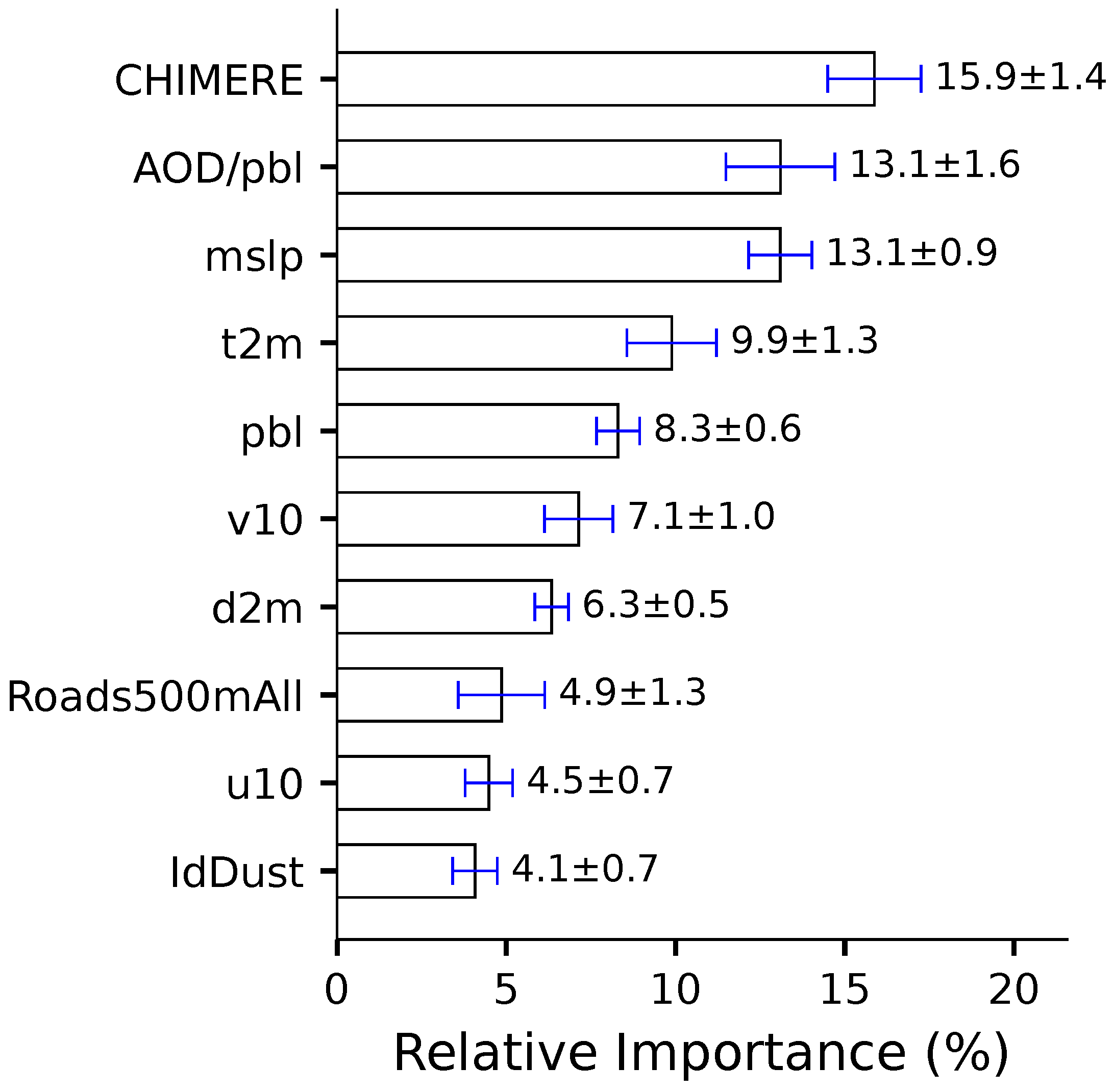
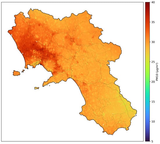
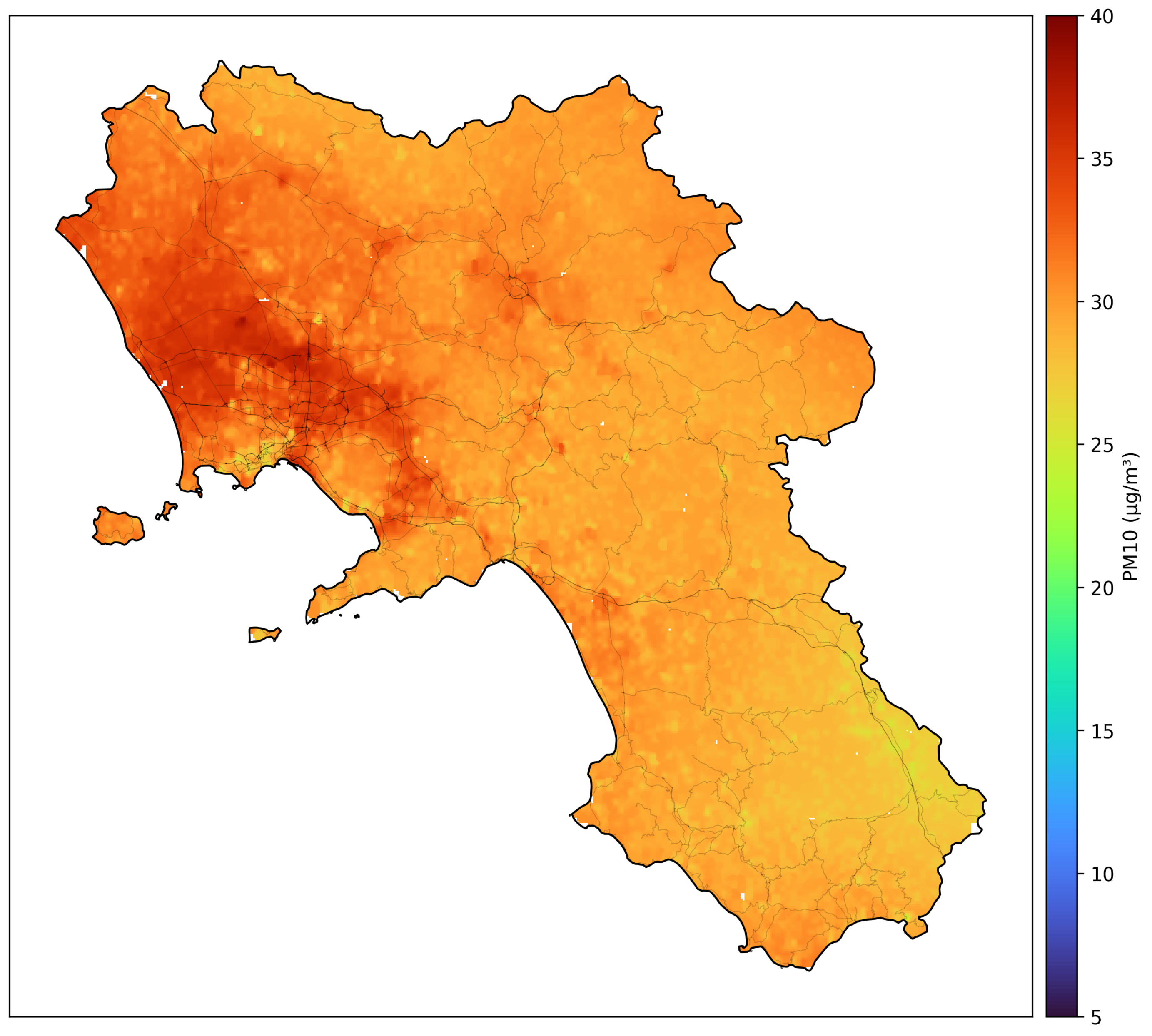
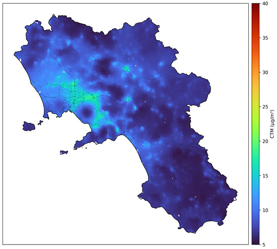
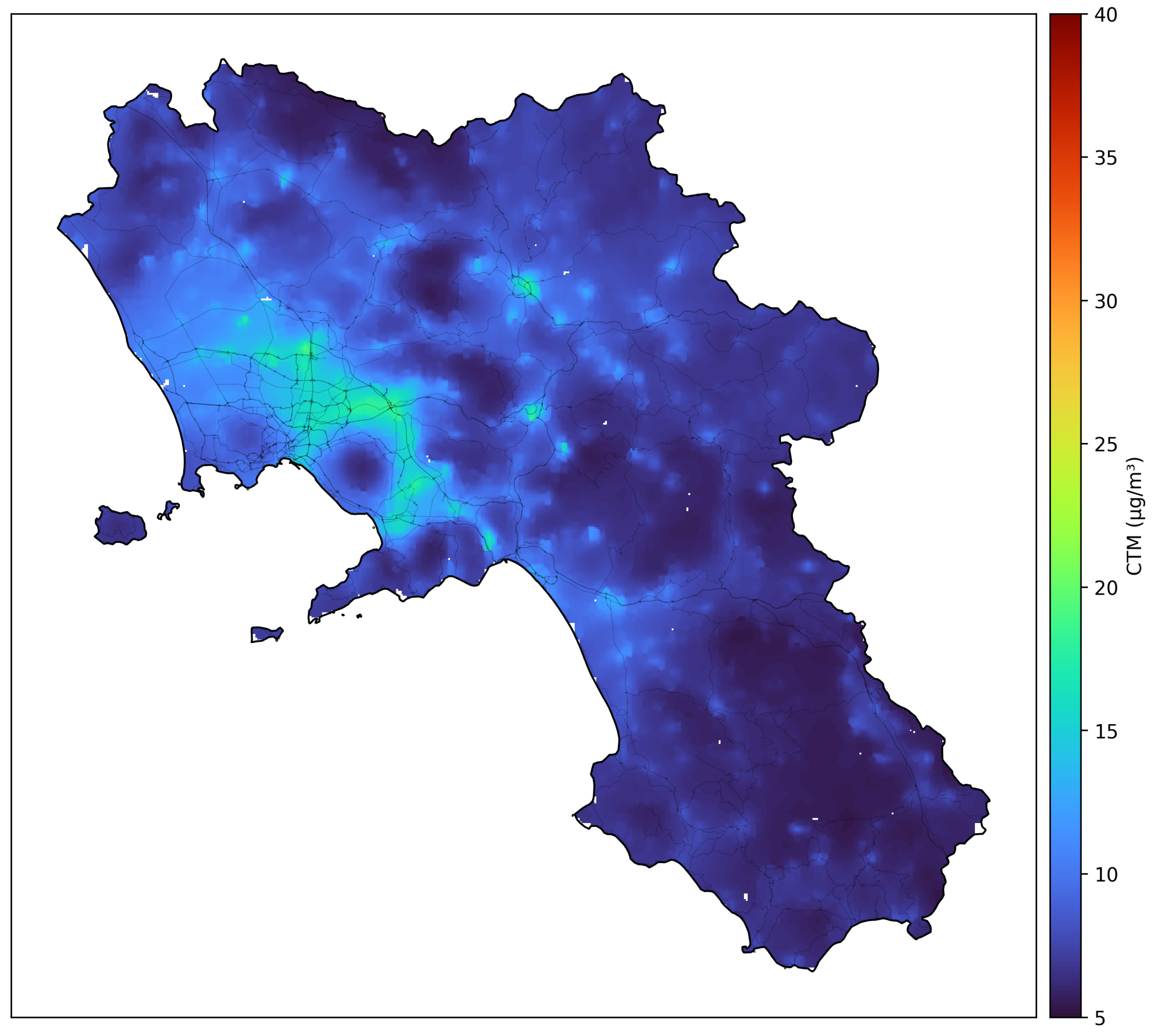
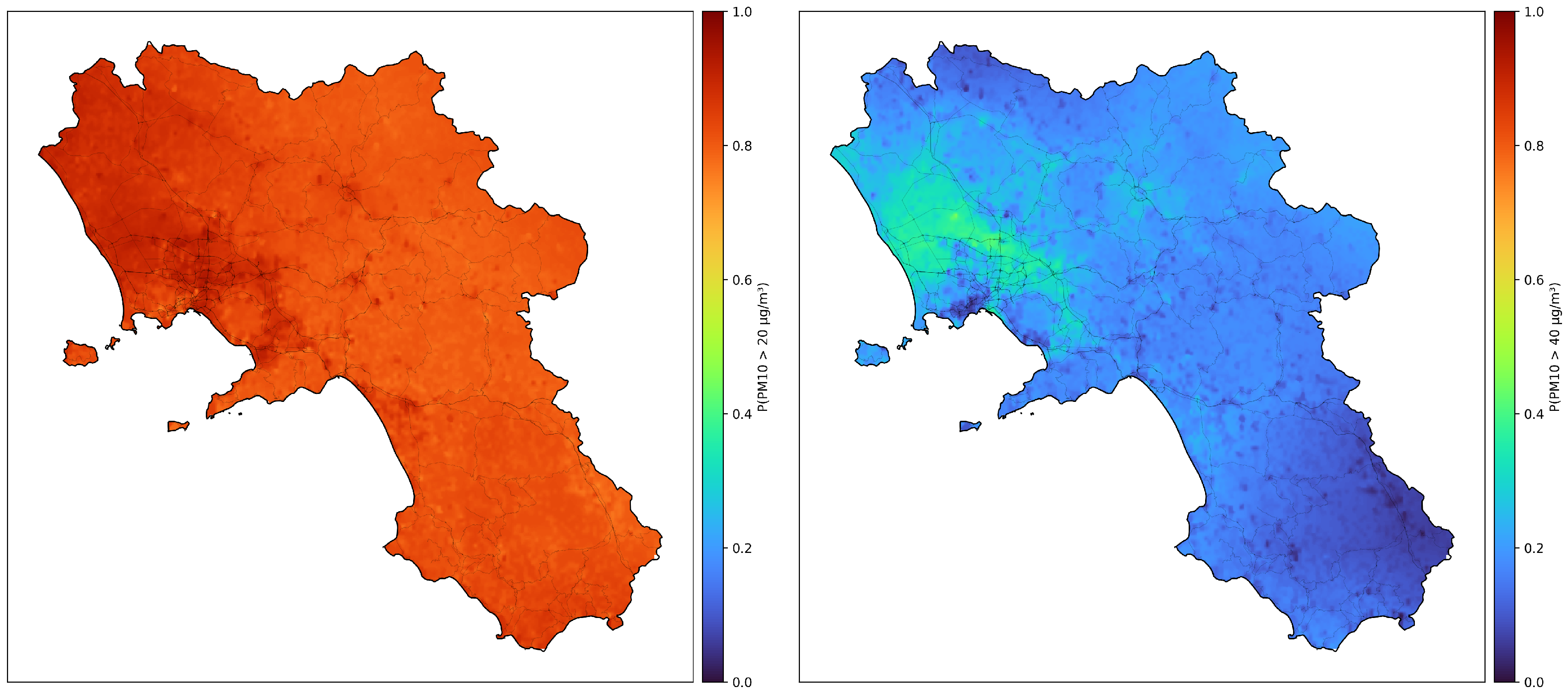
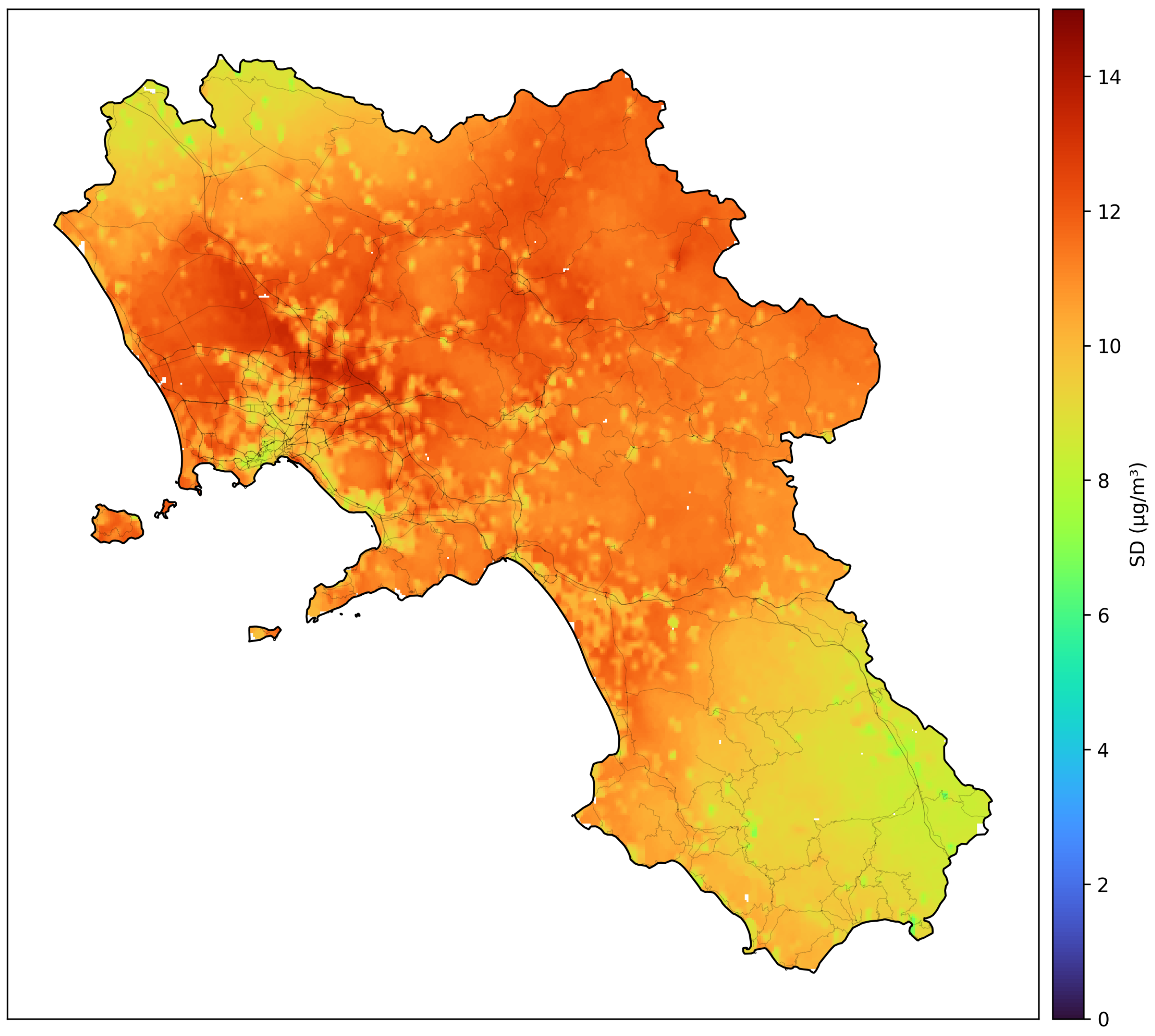

Disclaimer/Publisher’s Note: The statements, opinions and data contained in all publications are solely those of the individual author(s) and contributor(s) and not of MDPI and/or the editor(s). MDPI and/or the editor(s) disclaim responsibility for any injury to people or property resulting from any ideas, methods, instructions or products referred to in the content. |
© 2026 by the authors. Licensee MDPI, Basel, Switzerland. This article is an open access article distributed under the terms and conditions of the Creative Commons Attribution (CC BY) license.