Informer-Based Precipitation Forecasting Using Ground Station Data in Guangxi, China

Abstract

Precipitation forecasting is essential for disaster prevention, water resource management, and socio-economic resilience. The field has evolved from numerical weather prediction (NWP) and optical-flow-based methods toward data-driven deep learning approaches that can exploit larger observational datasets and model complex nonlinear relationships. Against this background, this study evaluates multi-station temporal forecasting models within a single-year, station-based proof-of-concept benchmark under unified data conditions. We adapt the Transformer and Informer architectures to this meteorological setting, rigorously preprocess the AWS dataset to avoid data leakage, and select predictive variables using complementary linear and nonlinear relevance criteria. Model performance is assessed using continuous and categorical precipitation metrics, including the Critical Success Index (CSI). The results show that the Informer outperforms the recurrent neural network (RNN) baselines and achieves the lowest mean MAE and RMSE together with the highest mean CSI among the evaluated models while using substantially fewer parameters than the standard Transformer. However, its sample-wise absolute error distribution remains statistically comparable to that of the standard Transformer. Overall, this study establishes a single-year, station-based proof-of-concept benchmark for comparing architectures in very-short-term (1–5 h ahead) precipitation forecasting.

1. Introduction

Precipitation forecasting is essential for disaster mitigation, water resource management, and socio-economic planning [1]. In China, accurate rainfall prediction is particularly important for flood and drought preparedness [2]. Automatic Weather Stations (AWSs) provide dense, routinely updated meteorological observations, including pressure, temperature, humidity, wind, sunshine duration, cloud cover, air quality, and precipitation [3]. These multivariate observations form a valuable basis for real-time forecasting and for subsequent data-driven studies. As a result, meteorological agencies have increasingly developed forecasting systems based on observational data, opening new opportunities for precipitation prediction [4].

Meteorological observations from multiple AWSs inherently contain both spatial and temporal information. They also include heterogeneous variables, such as geographic coordinates, pressure, humidity, and temperature-related indices, which together define a high-dimensional prediction problem. Earlier approaches largely relied on feature engineering to construct relationships between predictors and rainfall. More recently, deep learning methods such as convolutional neural networks (CNNs) [5] and recurrent neural networks (RNNs) [6] have provided new solutions for precipitation forecasting. In our previous work, for example, CNN-based models were used for cumulonimbus distribution forecasting, a task closely related to rainfall prediction [7]. However, as input dimensionality and forecasting horizons increase, the representational capacity of conventional models becomes more limited, motivating the exploration of more expressive architectures.

The Transformer is built on self-attention and is therefore well suited to long multivariate sequences because it supports parallel computation and flexible dependency modeling [8]. Transformer-based architectures have shown strong performance in natural language processing, computer vision, and time-series prediction [6,9,10]. More broadly, attention-based models have delivered competitive results across a wide range of multivariate time-series tasks and data conditions [11,12,13,14,15].

Recent studies have also explored hybrid designs that combine Graph Neural Networks (GNNs) with Transformers for traffic forecasting and multimodal prediction, highlighting the value of modeling both temporal structure and inter-station dependencies [11,16,17]. Nevertheless, research on pretrained Transformers for time series remains relatively limited, and much of the existing work has focused on classification rather than forecasting [18]. It is also important to distinguish station-based tabular forecasting from radar- or satellite-based nowcasting: the latter is primarily concerned with spatial extrapolation, whereas the former must model continuous multivariate physical sequences recorded at stations. Although graph and hybrid models are promising, they often rely on explicitly defined station topologies or rich spatial adjacency information that may not be readily available. In this study, we therefore examine the feasibility of Transformer-family architectures on large-scale AWS sequence data and position the analysis as a single-year, station-based proof-of-concept benchmark for architecture comparison under unified data conditions.

A ConvLSTM-based model has been developed for short-range precipitation forecasting during the Indian Summer Monsoon, showing that multivariable deep learning can provide competitive forecasting skill [19]. A subsequent CNN-LSTM framework for weather forecasting reported improved performance relative to a CNN-GRU baseline while maintaining reasonable computational cost [20]. In our own earlier work, we introduced a GCN-TrajGRU-attention framework for cumulonimbus cloud prediction from radar echo data in subtropical regions [5]. Transformer-based vision models have also demonstrated potential for short-term weather forecasting through a modified UNet with 3D shifted-window Transformers [21].

Vanilla Transformers face limitations in long-sequence time-series forecasting because of quadratic computational complexity, heavy memory consumption, and encoder-decoder inefficiency [22]. To address these issues, the Informer architecture introduced ProbSparse self-attention and a generative decoder for more efficient long-sequence forecasting [22]. Subsequent studies have applied Informer-type encoders to problems such as tool-wear prediction [23] and high-missing-rate time-series imputation [24], suggesting that the architecture is effective in extracting global temporal features under challenging sequence conditions.

In summary, although Transformer-based models have been widely studied in long-sequence forecasting, their application to station-based meteorological forecasting remains comparatively limited, especially for precipitation prediction. The present study therefore evaluates Transformer and Informer on the AWS dataset under a unified experimental setting.

2. Method

2.1. Transformer

The Transformer is built on the attention mechanism and uses multi-head self-attention to encode the input sequence and decode the output sequence. Unlike recurrent neural networks (RNNs), convolutional neural networks (CNNs), and recursive neural networks (RecNNs), the Transformer processes the full sequence simultaneously, allowing contextual dependencies to be modeled more efficiently. In this study, these properties make the model well suited to long multivariate meteorological sequences and efficient parallel training.

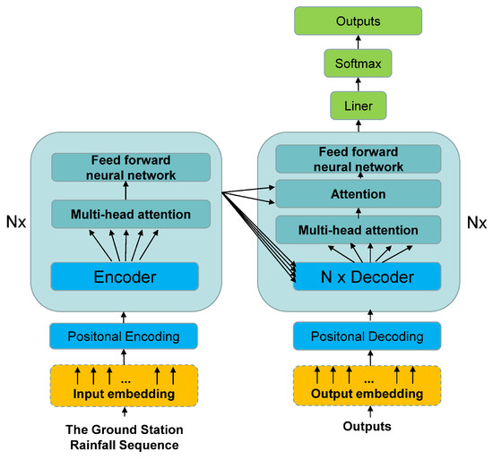
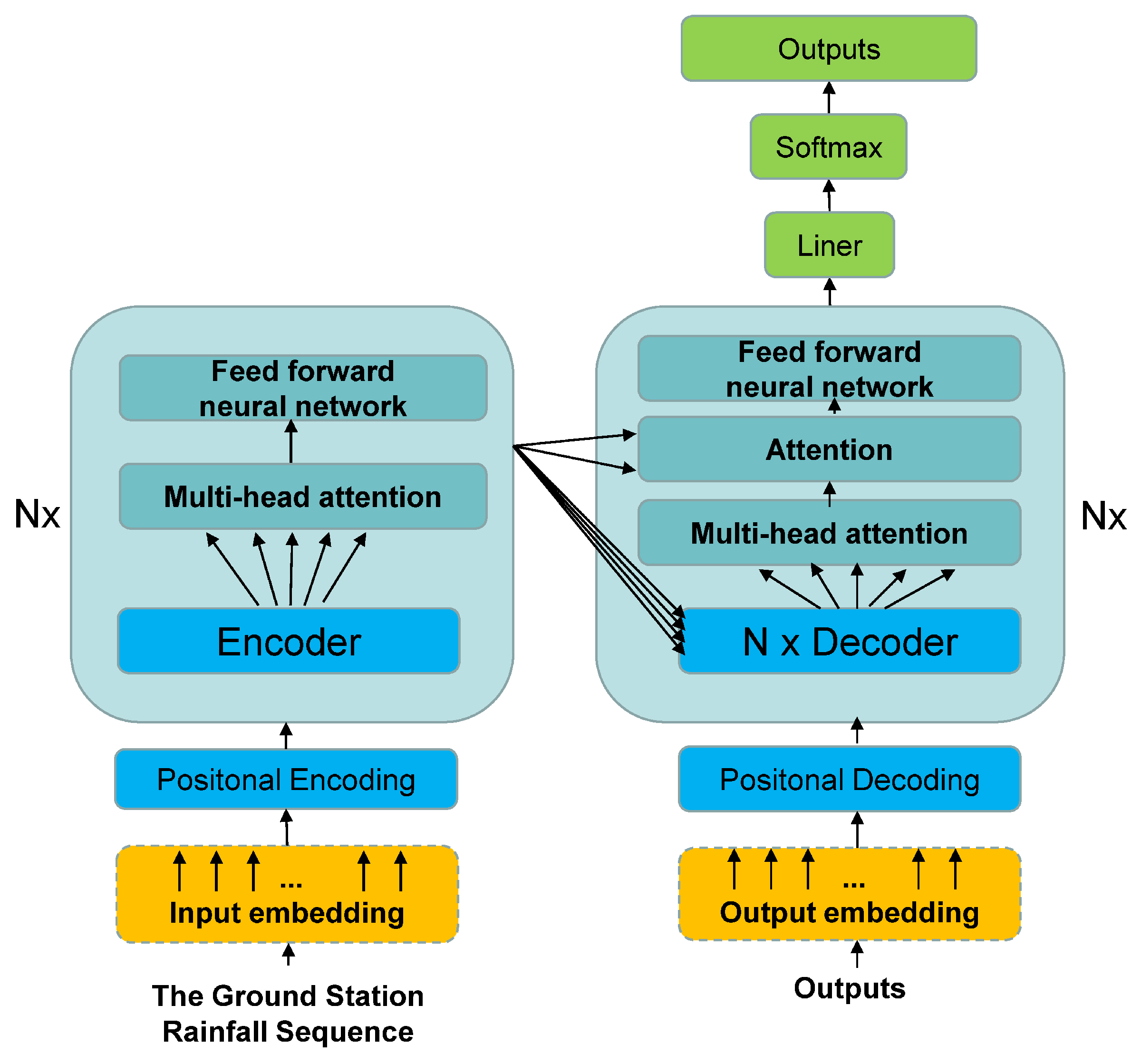
In this study, historical meteorological observations are used as input to the Transformer to predict near-future precipitation. As shown in Figure 1, the Transformer used in this study consists of an encoder and a decoder. Both are composed of multi-head attention modules and feed-forward layers. The encoder and decoder each contain $N=6$ repeated layers, and every layer includes two sub-layers: a multi-head self-attention block and a fully connected feed-forward network. Each sub-layer is followed by a residual connection and layer normalization, yielding the output shown in Equation (1):

$$Output=LayerNorm(x+Sublayer(x\left)\right)$$

(1)

Figure 1. The Structure of the Transformer.

The attention module takes three inputs, namely Query (Q), Key (K), and Value (V), and computes attention as follows:

$$\mathrm{Attention}(Q,K,V)=\mathrm{softmax}\left({\displaystyle \frac{Q{K}^T}{\sqrt{d}}}\right)V$$

(2)

The definitions of Q, K, and V are given in Equation (3):

$$\begin{array}{cc}\hfill Q& =W^{Q}X\hfill \\ \hfill K& =W^{K}X\hfill \\ \hfill V& =W^{V}X\hfill \end{array}$$

(3)

The attention value at a given time step is obtained from the similarity between its query vector and the keys at other time steps. In this way, the model can selectively retrieve relevant temporal information from the sequence. The scaling term reduces the variance of high-dimensional dot products and helps stabilize optimization [25].

As presented in Equations (3) and (5), multi-head attention applies h different linear transformations to the query, key, and value matrices to generate multiple attention heads, which are then concatenated into a single output representation.

$$\mathrm{MultiHead}(Q,K,V)=\mathrm{Concat}(hea{d}_1,\dots ,hea{d}_h)W^O$$

(4)

$$hea{d}_i=Attention(Q{W}_i^Q,K{W}_i^K,V{W}_i^V)$$

(5)

The Transformer model consists of two components, namely the encoder and the decoder, which share a similar input architecture. During inference, the decoder generates forecast values for future time steps from the encoded historical sequence and the previously generated outputs. In this forecasting setting, the encoder applies self-attention to the historical input sequence, whereas the decoder combines masked self-attention and encoder–decoder attention to produce temporally consistent predictions. During training, the decoder can use shifted ground-truth targets as context; during forecasting, it proceeds autoregressively because future observations are unavailable.

2.2. Informer

The Transformer has demonstrated strong performance in time-series forecasting. However, three limitations are particularly relevant in long-sequence settings: (1) self-attention has time and memory complexity of $O\left(L^2\right)$, where L is the sequence length; (2) memory consumption scales rapidly with the number of encoder and decoder layers; and (3) autoregressive decoding can slow inference.

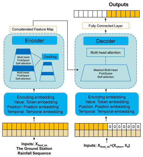
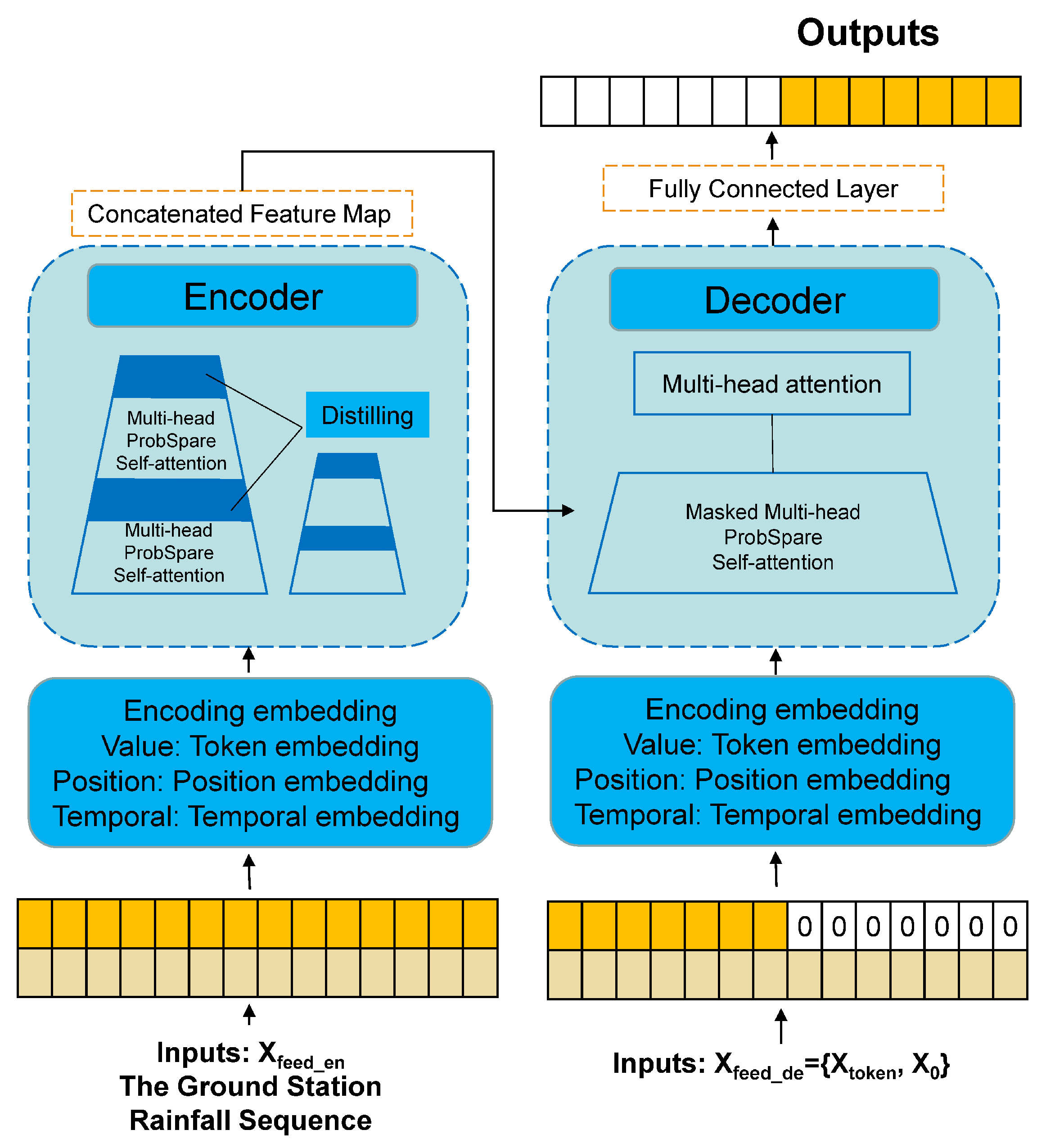
To address these issues, the Informer architecture was proposed with ProbSparse self-attention, thereby reducing time and memory complexity to $O\left(L\log L\right)$ [22]. In addition, self-attention distilling emphasizes dominant responses while shortening the input sequence passed to each successive layer, reducing the computational burden to $O\left(\right(2-ϵ\left)L\log L\right)$. The architecture also adopts a generative decoder that produces the forecast in a single forward pass. As shown in Figure 2, the main improvements introduced in Informer are summarized below.

Figure 2. The Structure of the Informer.

1.

As presented in Equation (6), ProbSparse self-attention ranks queries by importance and retains only the most influential top-u queries. By focusing computation on the dominant query-key interactions, the method improves efficiency while preserving the most informative dependencies.

$$\mathrm{Attention}(Q,K,V)=\mathrm{softmax}\left({\displaystyle \frac{Q{K}^T}{\sqrt{d}}}\right)V$$

(6)

2.

Self-attention distilling reduces the input sequence length at each layer and therefore lowers both computational cost and memory use. In practice, max-pooling with stride 2 compresses the representation passed to the next layer, allowing the model to focus on dominant information while handling long input sequences more efficiently.

3.

The generative decoder produces the target sequence in a single forward process rather than through step-by-step iterative decoding. This design improves memory efficiency and accelerates forecasting, especially for long sequences.

2.3. Data

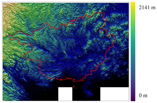
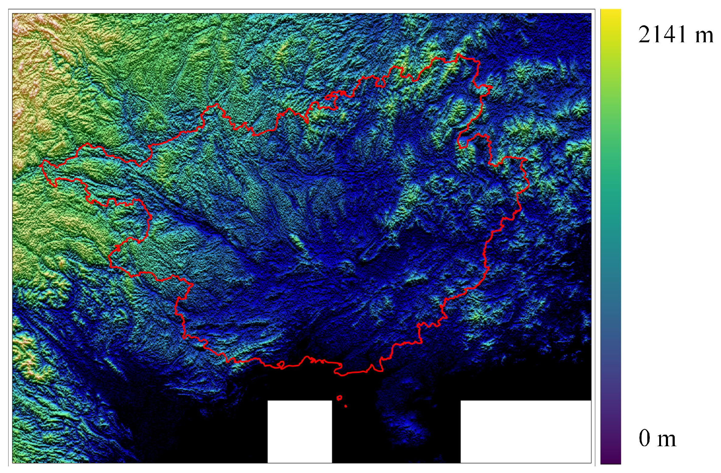
This study focuses on Guangxi (104° E–112° E, 21° N–27° N) and assesses the feasibility of hourly precipitation forecasting using observations collected at 2928 stations from January to October 2019. Guangxi is dominated by mountainous and hilly terrain and can be broadly divided into mountains, hills, plateaus, plains, rocky mountains, and water surfaces. Mountains above 800 m and low mountains between 400 and 800 m account for approximately 39.7% of the total land area, while hills between 200 and 400 m account for 10.3%. Landforms below 200 m, including valleys, piedmont plains, deltas, and low platforms, account for 26.9%, whereas water surfaces account for 3.4%. The topographic characteristics of Guangxi are shown in Figure 3.

Figure 3. DEM-Based Topographic Map of Guangxi. Colors Represent Surface Elevation from 0 m to 2141 m.

As shown in Figure 3, valleys and basins in Guangxi can generate local microclimates; therefore, topography may influence rainfall distribution through moisture trapping and rain-shadow effects.

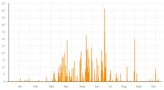
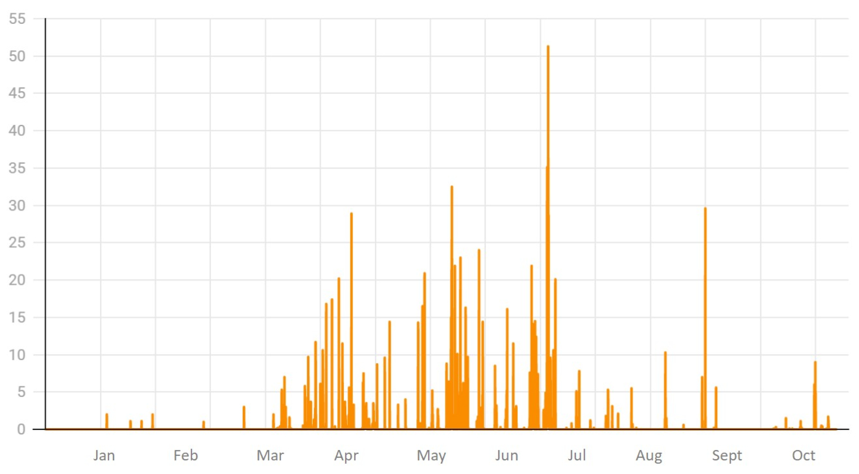
To characterize rainfall variability in 2019, we summarized the hourly precipitation records throughout the study period. As shown in Figure 4, rainfall occurred more frequently from March to September in Guangxi. During June, July, and August, most events were light to moderate, whereas heavy rainfall was relatively infrequent. Nevertheless, occasional intense downpours still occurred and posed substantial challenges for local communities and short-term disaster preparedness. After August, precipitation activity decreased.

Figure 4. Rainfall Records of Guangxi in 2019.

AWSs are automated observing sites equipped with sensors that measure variables such as pressure, precipitation, temperature, humidity, wind, sunshine duration, cloud cover, and air quality. These routinely updated observations can be used to characterize the occurrence and intensity of precipitation together with related meteorological conditions, thereby providing a reliable basis for data-driven weather forecasting [26].

Based on the above considerations, a dataset of hourly meteorological observations from sites across Guangxi was compiled. The dataset spans from 00:00 on 1 January 2019 to 23:00 on 30 October 2019. A summary of the raw surface observations is presented in Table 1.

Table 1. Summary of AWS Variables and Ranges.

Variable	Name	Definition	Unit	Range
station_ID	Station identifier	2928 stations in Guangxi	No.	59,053–846,805
Lat	Latitude	Station latitude	Degree	20°54′∼26°23′
Lon	Longitude	Station longitude	Degree	104°29′∼112°04′
PRS_Sea	Sea-level pressure	Air pressure reduced to sea level	hPa	995∼1024
PRS_Change_3h	3-h pressure change	Barometric pressure change over the previous 3 h	hPa	$-4.1$∼4.4
PRS_Change_24h	24-h pressure change	Barometric pressure change over the previous 24 h	hPa	$-7.7$∼8.8
TEM_Change_24h	24-h temperature change	Air-temperature change over the previous 24 h	°C	$-13.5$∼10.0
DPT	Dew-point temperature	Temperature at which saturation occurs at constant pressure and water vapor content	°C	3.4∼28.9
RHU	Relative humidity	Ratio of actual vapor pressure to saturation vapor pressure	%	20∼100
PRE_1h	1-h precipitation	Precipitation accumulated over the previous 1 h	mm	0∼250
PRE_3h	3-h precipitation	Precipitation accumulated over the previous 3 h	mm	0∼250

As summarized in Table 1, the dataset contains eleven hourly variables relevant to precipitation forecasting, including station identifiers, geographic coordinates, pressure-related variables, temperature-related variables, humidity, and recent precipitation history.

In practice, these observations were organized as multivariate time series, with rows representing hourly records and columns representing measured variables.

Ground station observations are generally regarded as one of the most reliable sources of near-surface meteorological information. Nevertheless, uneven station distribution, temporal gaps, erroneous values, and duplicated records can still degrade data quality in practice. Careful preprocessing of the raw AWS observations is therefore essential before model development [27].

2.4. Data Pre-Processing

Because of hardware and transmission limitations in the AWS system, some records contain abnormal placeholder values such as 9999 and 9998. These missing or abnormal values account for approximately 1.5% of the observations across all stations. In preprocessing, these values were first replaced with NaN and then filled by linear interpolation along the time dimension for each station and variable. This strategy preserves temporal continuity more naturally than simple mean imputation.

Initially, all eleven raw meteorological variables listed in Table 2 were considered. After data cleaning and feature screening, five predictors were retained for forecasting. Because these variables differ substantially in scale and physical units, direct use as model inputs would bias the optimization process. We therefore adopted min-max normalization rather than zero-mean standardization (Z-score). For sparse, non-negative precipitation variables, min-max scaling preserves the physical meaning of zero rainfall more naturally and avoids the negative artifacts introduced by centering. The normalization is defined as follows:

$$x^{\prime }={\displaystyle \frac{x-min\left(A\right)}{max\left(A\right)-min\left(A\right)}}$$

(7)

Here, $max(·)$ and $min(·)$ denote the maximum and minimum values of each variable. To prevent information leakage, these normalization parameters were estimated using only the training set and then applied unchanged to the validation and testing sets. This step places all predictors on a common scale, stabilizes optimization, and improves numerical efficiency during training.

Table 2. Minimum and Maximum Values of the Variables Listed in Table 1.

	PRS_Sea	PRS_Change_3h	PRS_Change_24h	TEM_Change_24h
Maximum	1024.2	4.4	8.8	10.0
Minimum	995.7	−4.1	−7.7	−13.5
	DPT	RHU	PRE_1h	PRE_3h
Maximum	28.9	100.0	51.3	101.6
Minimum	3.4	20.0	0.0	0.0

After these preprocessing steps, the dataset was screened for candidate predictors using Pearson correlation, Spearman rank correlation, and mutual information so that linear and nonlinear, as well as positive and negative, relationships could all be considered. The final feature set was selected according to both statistical relevance and meteorological interpretability. Mutual information was estimated using a k-nearest-neighbor (k-NN) approach in order to capture nonlinear dependence between continuous meteorological variables. The Pearson correlation coefficient is defined in Equation (8):

$$COR(X,Y)={\displaystyle \frac{{\sum }_i^n(X_i-\overline{X})(Y_i-\overline{Y})}{\sqrt{{\sum }_i^n{(X_i-\overline{X})}^2{\sum }_i^n{(Y_i-\overline{Y})}^2}}}$$

(8)

Equation (8) shows that the Pearson coefficient normalizes covariance by the standard deviations of the two variables. Unlike covariance, whose magnitude depends on the scale of the variables, the correlation coefficient is dimensionless and ranges from $-1$ to 1, making it easier to compare relationships across variables.

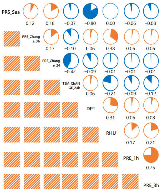
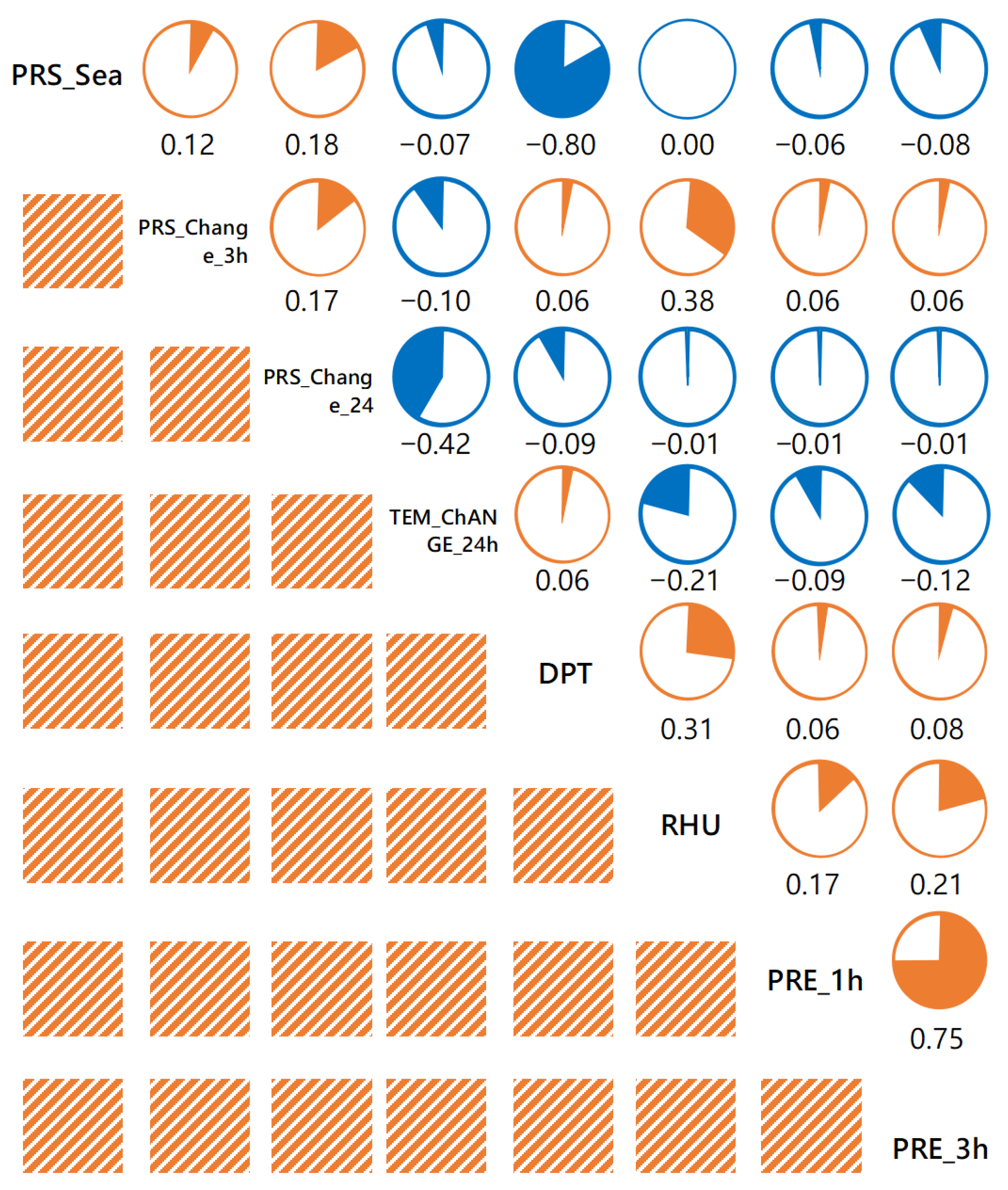
In Figure 5, the strength of the relationship between two variables can be interpreted from the coefficient magnitude. Values between 0.6 and 0.8 indicate strong correlation, values between 0.4 and 0.6 indicate moderate correlation, and values between 0.2 and 0.4 indicate weak correlation. Values close to zero suggest little or no linear relationship. Negative coefficients are equally important in meteorological analysis because they capture inverse physical relationships, such as pressure decreases preceding rainfall.

Figure 5. Pearson Correlation Coefficient Diagram.

As shown in Figure 5, sea-level pressure and its short-term changes exhibit only weak correlations with most of the other variables. By contrast, PRS_Change_3h shows a mild positive relationship with relative humidity, whereas TEM_Change_24h is negatively correlated with several predictors. Relative humidity is strongly correlated with dew point temperature and more moderately correlated with PRE_1h and PRE_3h. As expected, the strongest positive relationship is observed between PRE_1h and PRE_3h, with a Pearson coefficient of 0.75.

By combining Pearson correlation, Spearman correlation, and mutual information, we evaluated positive and negative associations together with potentially nonlinear relationships Table 3. A predictor was retained when it ranked consistently high in at least two of the three criteria, namely absolute Pearson correlation, absolute Spearman correlation, and mutual information. Under this rule, PRS_Change_3h, DPT, RHU, PRE_1h, and PRE_3h were selected. From a physical perspective, RHU and DPT are key moisture-related variables: high RHU indicates near-saturated conditions, whereas DPT reflects the absolute moisture content of the air. In a humid subtropical region such as Guangxi, both variables are particularly relevant to the initiation of short-term convective rainfall. By contrast, TEM_Change_24h showed limited statistical relevance in this dataset, which may reflect the fact that short-term moisture and pressure variations are more important than 24-h temperature change for the rainfall regimes examined here.

Table 3. Feature Selection Summary Using Multiple Criteria.

Variable	Pearson	Spearman	Mutual Info.	Decision
PRS_Sea	Low	Low	Low	Discard
PRS_Change_3h	Med	Med	Med	Retain
PRS_Change_24h	Low	Low	Low	Discard
TEM_Change_24h	Low	Low	Low	Discard
DPT	High	High	High	Retain
RHU	High	High	High	Retain
PRE_1h	High	High	High	Retain
PRE_3h	High	High	High	Retain

3. Experiment

3.1. Division of Datasets

After preprocessing, the data were converted to tensors and divided into training, validation, and testing sets. To preserve temporal causality and prevent data leakage, the split was strictly chronological, without random shuffling. As shown in Table 4, data from 1 January to 31 May 2019 were used for training, data from 1 June to 31 August 2019 were used for validation and hyperparameter tuning, and data from 1 September to 30 October 2019 were reserved for testing. Data loaders were constructed with batch sizes of 128 for training and 512 for testing. These settings were selected empirically to balance training efficiency and convergence stability.

Table 4. Detailed AWS Dataset Settings.

	Transformer and Informer Experiments
Number of Stations	2928
Predictor Variables	5
Training Period	01/01/2019–31/05/2019
Validation Period	01/06/2019–31/08/2019
Testing Period	01/09/2019–30/10/2019
Loss Function	MSE Loss
Evaluation Metric	MAE, MSE, RMSE, MAPE, CSI, POD, FAR

In the experiments, the previous 15 h of observations were used to forecast precipitation over the next 5 h at hourly intervals. Station records were updated hourly and provided to both the Transformer and Informer models. The encoder input dimension was eight, consisting of five retained meteorological predictors and three auxiliary temporal encoding terms. The decoder input dimension was seven, and the model generated precipitation forecasts for five future time steps. Multi-head attention was divided into eight heads, and both the encoder and decoder contained two layers Table 5.

Table 5. Overview of Hyperparameters and Model Settings.

Model	Layers	Hidden Size/${\mathit{d}}_{\mathit{model}}$	Heads	Parameters
LSTM	8	16	-	1369
GRU	8	16	-	1033
FNN	8	16	-	201
Transformer	2	32	8	119,297
Informer	2	32	8	38,305

3.2. Experimental Environment and Strategies

The models were implemented in Python 3.7 using PyTorch 1.7. All experiments were conducted on a Windows 10 workstation equipped with an Intel i5-9400F CPU and an NVIDIA RTX 2080Ti GPU. Following standard practice [28], we evaluated model performance using multiple complementary metrics.

All models were optimized using the mean square error (MSE) loss [28]. Given the size of the dataset, each method was trained for 150 epochs to ensure a fair and stable comparison. All baselines were tuned on the same validation set with comparable search budgets. For each epoch, the average loss across iterations was recorded, and the final model evaluation was conducted on the testing set.

To evaluate forecasting performance, we used mean absolute error (MAE, Equation (9)), mean square error (MSE, Equation (10)), root mean square error (RMSE, Equation (11)), and mean absolute percentage error (MAPE, Equation (12)). We also used three categorical precipitation metrics: Critical Success Index (CSI), Probability of Detection (POD), and False Alarm Ratio (FAR). For categorical verification, a threshold of 0.1 mm/h was used to define a measurable precipitation event. This threshold distinguishes rainy from non-rainy conditions rather than heavy rainfall. To complement this binary verification, we further examined model behavior under higher rainfall thresholds and through a continuous extreme-event case study (Figure 7).

$$MAE={\displaystyle \frac{1}{n}}\sum _{i=1}^n\left|{Predicted}_i-{Actual}_i\right|$$

(9)

$$MSE={\displaystyle \frac{1}{n}}\sum _{i=1}^n{({Predicted}_i-{Actual}_i)}^2$$

(10)

$$RMSE=\sqrt{{\displaystyle \frac{{\sum }_{i=1}^n{({Predicted}_i-{Actual}_i)}^2}{n}}}$$

(11)

$$MAPE={\displaystyle \frac{1}{n}}\sum _{i=1}^n\left|{\displaystyle \frac{{Actual}_i-{Predicted}_i}{{Actual}_i+ϵ}}\right|$$

(12)

where a small constant $ϵ$ is added to the denominator to avoid division by zero. Because precipitation data contain many near-zero values, MAPE can be disproportionately inflated and should therefore be interpreted together with absolute error metrics.

For categorical precipitation evaluation, events are classified as Hits (H), Misses (M), and False Alarms (F) using a predefined threshold. The metrics are defined as follows:

$$CSI={\displaystyle \frac{H}{H+M+F}}$$

(13)

$$POD={\displaystyle \frac{H}{H+M}}$$

(14)

$$FAR={\displaystyle \frac{F}{H+F}}$$

(15)

3.3. Experiment Results and Analysis

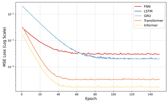
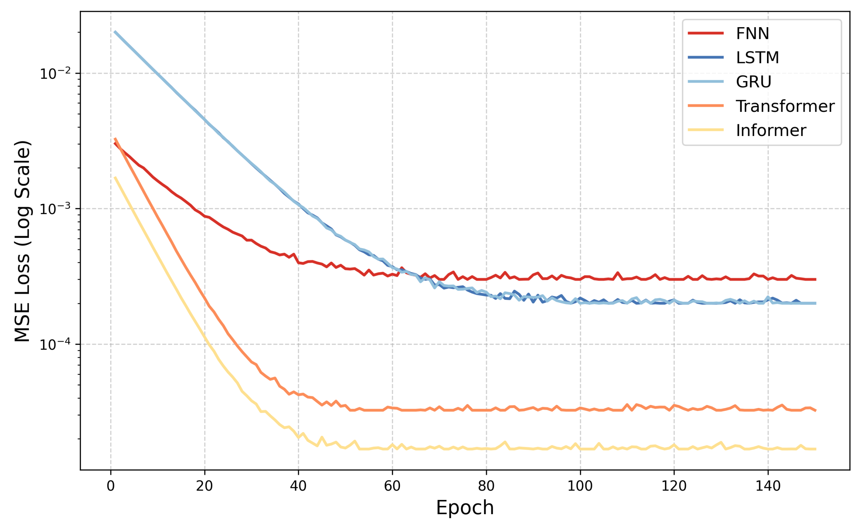
Figure 6 shows that the Informer converged more smoothly than the standard Transformer during training. This behavior may be related to Informer’s distilling strategy and generative decoding design, although a dedicated ablation study is beyond the scope of the present work. The Informer also achieved a lower final loss value.

Figure 6. Convergence of Different Methods.

After training, all models were evaluated on the AWS testing set. The average performance over three independent runs is reported in Table 6. Overall, the attention-based models outperformed the baseline networks. In terms of continuous errors, the Transformer and Informer achieved consistently lower MAE and RMSE than LSTM, GRU, and FNN. For categorical verification, LSTM, GRU, and FNN showed very high false alarm ratios (FAR > 0.89) and low CSI values (≤0.10), indicating a tendency to overpredict rainfall. By contrast, the Transformer and Informer improved CSI while reducing FAR, suggesting better discrimination between actual precipitation events and false alarms. Among the two attention-based models, the Informer achieved the lowest mean MAE and RMSE and the highest mean CSI, while using substantially fewer parameters than the standard Transformer (38,305 versus 119,297). Nevertheless, as shown by the paired Wilcoxon test below, its sample-wise absolute error distribution remained statistically comparable to that of the standard Transformer.

Table 6. Experimental Results of Different Methods (Mean ± Std over 3 Runs).

	MAE	MSE	RMSE	MAPE	CSI	POD	FAR
FFN (8 layers)	$0.0123\pm 0.0024$	$0.0003\pm 0.0001$	$0.0157\pm 0.0024$	$5.3211\pm 1.2349$	$0.0719\pm 0.0038$	$0.9828\pm 0.0243$	$0.9280\pm 0.0040$
LSTM (8 layers)	$0.0081\pm 0.0045$	$0.0002\pm 0.0001$	$0.0148\pm 0.0021$	$2.6597\pm 2.6663$	$0.0686\pm 0.0008$	$0.8129\pm 0.2646$	$0.9292\pm 0.0022$
GRU (8 layers)	$0.0066\pm 0.0003$	$0.0002\pm 0.0000$	$0.0126\pm 0.0013$	$1.1069\pm 0.3238$	$0.1026\pm 0.0115$	$0.7333\pm 0.0106$	$0.8933\pm 0.0125$
Transformer	$0.0093\pm 0.0077$	$0.0002\pm 0.0003$	$0.0118\pm 0.0091$	$0.7591\pm 0.3863$	$0.1107\pm 0.0246$	$0.7828\pm 0.2461$	$0.8838\pm 0.0241$
Informer	$\mathbf{0}.\mathbf{0023}\pm \mathbf{0}.\mathbf{0002}$	$\mathbf{0}.\mathbf{0000}\pm \mathbf{0}.\mathbf{0000}$	$\mathbf{0}.\mathbf{0057}\pm \mathbf{0}.\mathbf{0001}$	$\mathbf{0}.\mathbf{4110}\pm \mathbf{0}.\mathbf{2344}$	$\mathbf{0}.\mathbf{1823}\pm \mathbf{0}.\mathbf{0628}$	$0.9333\pm 0.0501$	$\mathbf{0}.\mathbf{8148}\pm \mathbf{0}.\mathbf{0648}$

To further assess robustness across rainfall intensities, we computed CSI, POD, and FAR at thresholds of 1.0, 5.0, and 10.0 mm/h. The results are summarized in Table 7. The baseline models deteriorated rapidly as the rainfall threshold increased. In contrast, the Informer retained higher skill than the baseline models, with CSI values of $0.8757$ at 5.0 mm/h and $0.7133$ at 10.0 mm/h. It also outperformed the standard Transformer at these thresholds, although the 10.0 mm/h results should be interpreted with caution due to the limited number of positive events.

Table 7. Categorical Metrics Under Varying Precipitation Thresholds (Mean ± Std over 3 Runs).

Model	Threshold: ≥1.0 mm/h			Threshold: ≥5.0 mm/h			Threshold: ≥10.0 mm/h
	CSI	POD	FAR	CSI	POD	FAR	CSI	POD	FAR
FFN	$0.0391\pm 0.0160$	$0.9147\pm 0.0842$	$0.9608\pm 0.0160$	$0.1333\pm 0.1886$	$0.1556\pm 0.2200$	$0.0877\pm 0.1241$	$0.0595\pm 0.0842$	$0.0667\pm 0.0943$	$0.1250\pm 0.1768$
LSTM	$0.0184\pm 0.0130$	$0.6080\pm 0.4312$	$0.9816\pm 0.0130$	$0.0000\pm 0.0000$	$0.0000\pm 0.0000$	$0.0000\pm 0.0000$	$0.0000\pm 0.0000$	$0.0000\pm 0.0000$	$0.0000\pm 0.0000$
GRU	$0.1360\pm 0.0618$	$0.5547\pm 0.1619$	$0.8492\pm 0.0672$	$0.0632\pm 0.0635$	$0.1000\pm 0.1080$	$0.8565\pm 0.1118$	$0.0244\pm 0.0345$	$0.0400\pm 0.0566$	$0.6140\pm 0.4389$
Transformer	$0.5327\pm 0.0897$	$0.7813\pm 0.0983$	$0.3296\pm 0.1935$	$0.6839\pm 0.0020$	$0.8056\pm 0.0208$	$0.1798\pm 0.0194$	$0.4195\pm 0.0223$	$0.5867\pm 0.0189$	$0.4050\pm 0.0268$
Informer	$\mathbf{0}.\mathbf{5811}\pm \mathbf{0}.\mathbf{1195}$	$\mathbf{0}.\mathbf{8907}\pm \mathbf{0}.\mathbf{0360}$	$\mathbf{0}.\mathbf{3658}\pm \mathbf{0}.\mathbf{1561}$	$\mathbf{0}.\mathbf{8757}\pm \mathbf{0}.\mathbf{0070}$	$\mathbf{0}.\mathbf{9000}\pm \mathbf{0}.\mathbf{0136}$	$\mathbf{0}.\mathbf{0295}\pm \mathbf{0}.\mathbf{0157}$	$\mathbf{0}.\mathbf{7133}\pm \mathbf{0}.\mathbf{0701}$	$\mathbf{0}.\mathbf{7333}\pm \mathbf{0}.\mathbf{0822}$	$\mathbf{0}.\mathbf{0327}\pm \mathbf{0}.\mathbf{0233}$

Note: Categorical verification was performed point-wise across all five forecast horizons of the 896 complete test windows, yielding 4480 evaluated forecast points. The numbers of observed positive events for thresholds of 1.0, 5.0, and 10.0 mm/h were 125, 60, and 25, respectively.

To assess statistical significance, we conducted a Wilcoxon signed-rank test on sample-wise mean absolute errors. Specifically, we performed a paired two-sided test on the absolute errors from the test loader generated with the same chronological split and windowing scheme ($n=896$ complete sequence windows), where each paired unit corresponded to a sequence-level error from two models. The Informer was compared separately with GRU and with the standard Transformer. In addition to p-values, we report rank-biserial correlation as an effect-size measure. The Informer-versus-GRU comparison yielded $p<0.05$ (e.g., $p\approx 5.75\times {10}^{-147}$) with a rank-biserial correlation of approximately $0.99$, whereas the comparison with the standard Transformer yielded $p=0.403$ and a rank-biserial correlation of approximately $-0.08$. These results indicate that the Informer significantly outperforms the RNN baselines, but remains statistically comparable to the standard Transformer in terms of sample-wise absolute error distribution. This sample count differs from the categorical verification counts because the Wilcoxon analysis uses one paired error per sequence window, whereas Table 6 and Table 7 evaluate precipitation events point-wise across all forecast horizons from the same windows.

Finally, to evaluate accumulation consistency, we compared the sum of the first three 1-h forecasts with the observed 3-h accumulated precipitation. The results are presented in Table 8. For the Informer, the mean absolute discrepancy $\left|{\sum }_{k=1}^3{PR\hat{E}\_1h}_k-PRE\_3h^{obs}\right|$ was $1.56$ mm, which is lower than that of the baseline models and suggests better physical consistency with the observed accumulation. Incorporating explicit physical constraints into the loss function remains an important direction for future work.

Table 8. Physical Accumulation Consistency: Discrepancy Between the 3-Hour Sum of 1-Hour Forecasts and Observed 3-Hour Precipitation (mm).

Model	Mean Absolute Discrepancy	Median Discrepancy	90th Percentile Discrepancy
FFN	$2.43$	$0.98$	$5.67$
LSTM	$2.21$	$0.85$	$5.12$
GRU	$1.95$	$0.72$	$4.58$
Transformer	$1.72$	$0.61$	$4.03$
Informer	1.56	0.52	3.65

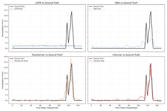
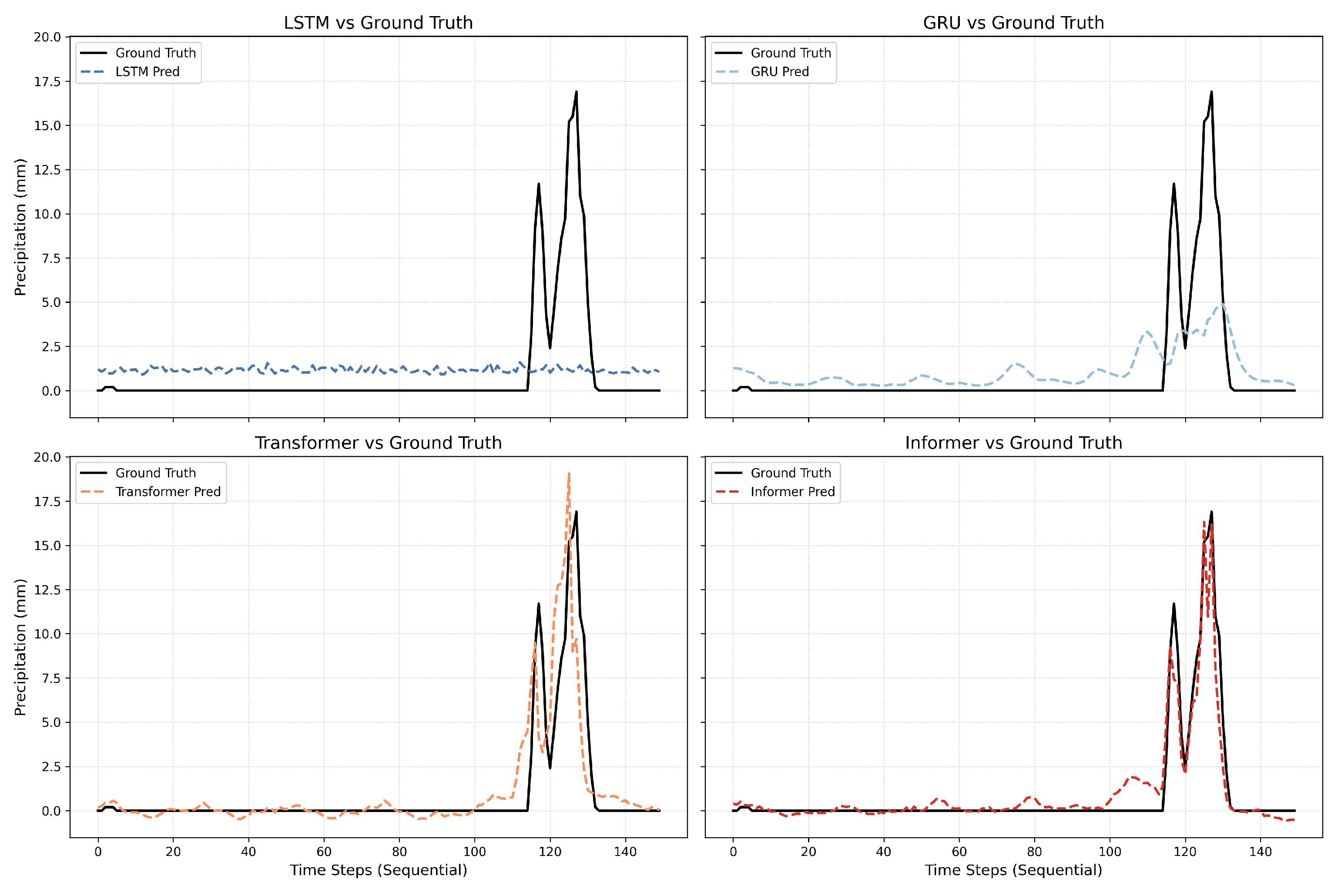
To further illustrate model behavior, we evaluated the trained models on a continuous forecasting segment from the test set. Specifically, we selected a 150-h window associated with an extreme rainfall event and compared the model predictions with the corresponding ground truth. The results for all baseline models and the attention-based models are shown in Figure 7. Notably, the Informer and Transformer tracked the major precipitation peaks more closely, whereas the RNN-based models and the FFN struggled to follow the abrupt changes.

Figure 7. Results of Continuous Extreme-Precipitation Forecasting.

This case study also highlights the remaining difficulty of forecasting extreme precipitation. Although the Informer reproduced the timing of the main peaks more faithfully than the recurrent baselines, some amplitude deviations remained, especially around the sharpest transitions. This behavior is consistent with the threshold-based evaluation in Table 7: performance remains comparatively strong at higher rainfall intensities, but the most extreme events are still difficult because they are rare, highly intermittent, and represented by only a limited number of positive samples in the present test set. The continuous extreme-event analysis should therefore be interpreted as evidence of improved relative skill rather than as evidence that extreme-rainfall forecasting has been fully solved. In addition, this case study represents only one continuous extreme-rainfall segment from the test period and should therefore be regarded as illustrative rather than exhaustive. A more complete assessment of extreme-event skill would require event-stratified statistics over a larger number of rare high-intensity cases.

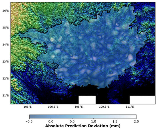
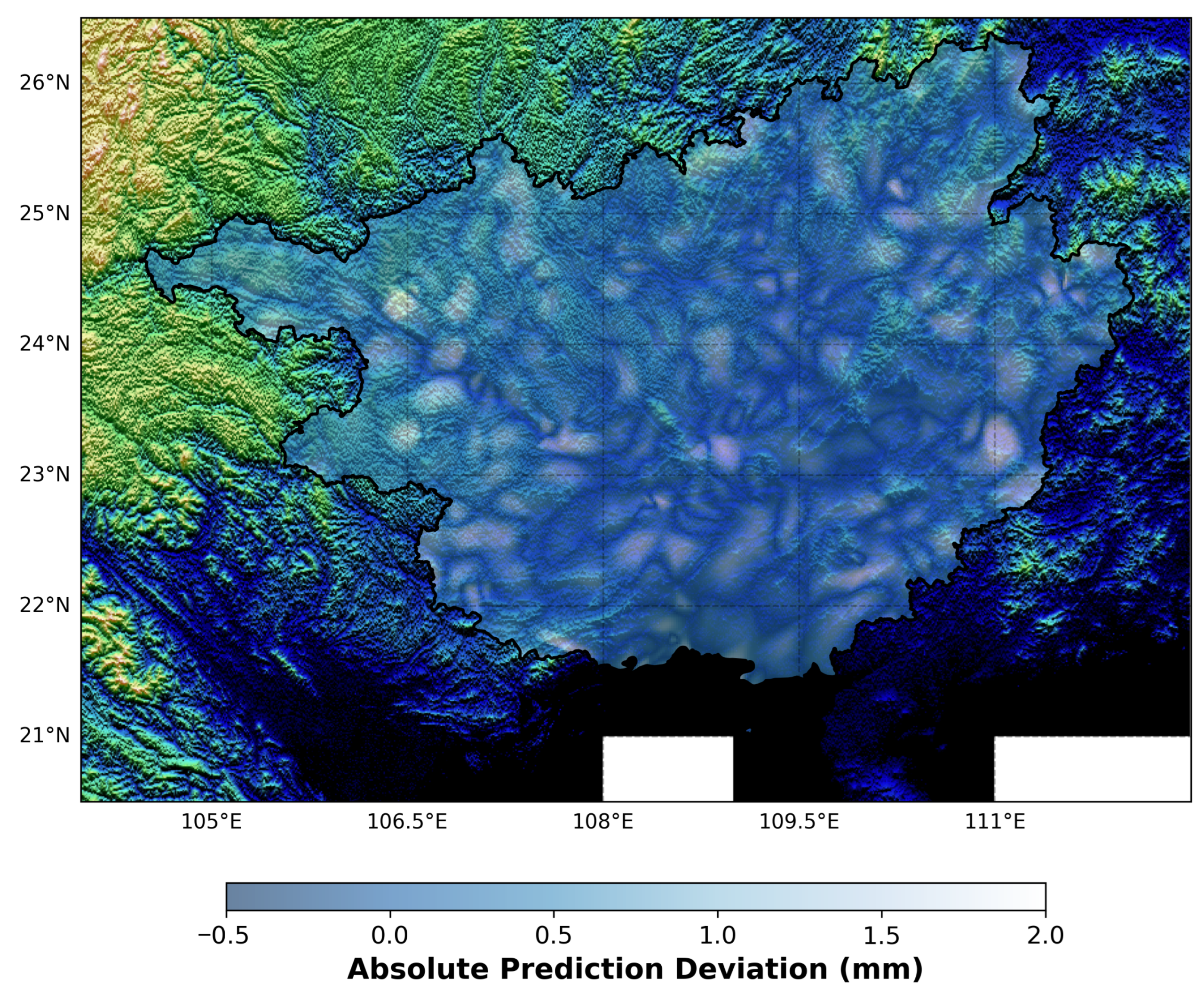
To complement the temporal evaluation, we further examined the spatial distribution of prediction errors across Guangxi. Figure 8 presents a continuous error heatmap produced by Kriging/Griddata interpolation and overlaid on a 3D digital elevation model (DEM). Compared with a point-based visualization, this representation provides a clearer view of the regional error pattern within the administrative boundary. Some larger errors appear over areas with more complex terrain, although this visual tendency should be interpreted cautiously because no formal terrain-stratified analysis was conducted. Overall, the figure provides a spatially interpretable summary of model error while also highlighting the challenges posed by complex topography.

Figure 8. Spatial Distribution of Absolute Prediction Deviation (mm) for the Informer Model Across the Guangxi Testing Set, Generated via Kriging Interpolation over a High-Resolution 3D DEM Background.

3.4. Discussion and Limitations

Although the proposed Informer model shows strong skill in precipitation forecasting, the results should be interpreted in light of several physical and modeling limitations.

First, the current architecture treats the data from 2928 meteorological stations primarily as multivariate time series. Although this design captures temporal evolution effectively, it does not explicitly encode the topological or spatial dependencies between stations, for example through Graph Neural Networks or spatial attention mechanisms. The spatial error heatmap in Figure 8 is therefore descriptive rather than evidence that the model has learned terrain-driven moisture transport. This point is important when comparing the present benchmark with ConvLSTM-style nowcasting systems, graph-based station models, and other hybrid spatial–temporal frameworks reported in the literature, because those approaches are designed to exploit spatial adjacency or image-like structure more directly. More specifically, ConvLSTM-style nowcasting models are typically designed for gridded radar or image-like inputs and are well suited to spatial extrapolation problems, whereas graph-based station models explicitly encode inter-station connectivity through predefined or learned graph structures. By contrast, the present study focuses on multivariate AWS sequences under a unified station-based benchmark and therefore emphasizes temporal representation learning rather than explicit spatial dependency modeling. Accordingly, the current results should not be interpreted as evidence that attention-based temporal models are universally superior to spatial or hybrid architectures, but rather as evidence that they provide competitive temporal forecasting skill under the current AWS setting. Hybrid spatial–temporal architectures, particularly GNN-enhanced station models, remain an important direction for future work.

Second, the feature-selection procedure prioritized variables with strong statistical relevance, such as RHU, DPT, and PRE_1h. However, precipitation in humid subtropical regions such as Guangxi is also influenced by broader thermodynamic and dynamical controls, including moisture convergence and vorticity. The exclusion of variables such as 24-h temperature change (TEM_Change_24h), although statistically justified in this dataset, may therefore simplify some convective triggers. Additional analyses stratified by altitude and terrain category would help clarify model behavior under different topographic conditions.

Third, the model outputs are not explicitly constrained by physical conservation laws. Enforcing accumulation consistency, for example by requiring 1-h forecasts to remain consistent with 3-h totals, would help reduce physically implausible precipitation behavior.

Finally, the temporal coverage of the dataset is limited to a single year (2019). The present study should therefore be interpreted as a proof-of-concept benchmark under a high-frequency single-year AWS setting, with the primary goal of comparing model architectures under unified data conditions rather than establishing a long-term climatological forecasting system. Even within these boundaries, the benchmark remains scientifically useful because it provides a controlled comparison of recurrent and attention-based architectures under the same preprocessing, splitting, and evaluation protocol. At the same time, the strong seasonality and non-stationarity of precipitation in Guangxi mean that the present results cannot be taken as evidence of long-term robustness across distinct climatic regimes. This architecture-oriented perspective helps identify which model classes merit further development before more demanding multi-year, terrain-stratified, and physics-constrained extensions are pursued. Future work should extend the analysis to multi-year datasets, more diverse climatic regimes, and loss functions that incorporate explicit physical constraints.

4. Conclusions

This study establishes a station-based benchmark for near-term precipitation forecasting based on AWS observations from Guangxi. The results support three main conclusions. First, rigorous chronological splitting and training-set-only normalization provide a leakage-resistant framework for comparing forecasting architectures under unified data conditions. Second, the retained predictors, selected through complementary linear and nonlinear criteria, highlight the importance of moisture-related variables such as RHU and DPT for short-term rainfall forecasting in Guangxi. Third, attention-based models show clear advantages for this task. In particular, the Informer achieved the lowest mean MAE and RMSE and the highest mean CSI among the evaluated models while requiring only about one-third of the parameters of the standard Transformer. The paired Wilcoxon test further showed that its sample-wise absolute error distribution remained statistically comparable to that of the standard Transformer, whereas its categorical detection was stronger at higher rainfall thresholds; however, the highest-threshold results should be interpreted cautiously because of the limited number of positive events. Overall, these findings indicate that efficient self-attention architectures such as Informer provide a compact and competitive solution for very-short-term (1–5 h ahead) precipitation forecasting under the present single-year AWS benchmark.

Despite these encouraging results, the present analysis remains limited by the temporal span of the dataset. The experiments use high-frequency hourly observations from a single year (2019) and do not yet incorporate explicit physical or spatial constraints. Given the strong seasonality and non-stationarity of precipitation, the study is best interpreted as a proof-of-concept comparison of model architectures, and its conclusions should not be generalized beyond the present benchmark without further multi-year validation. Therefore, the current findings are most appropriate for architecture benchmarking and methodological comparison, rather than for direct claims of operational robustness or climatological generalizability. Future work should extend the benchmark to multi-year datasets and include more detailed month-wise and terrain-stratified evaluations in order to better assess long-term robustness and generalizability.

References

- Ghamariadyan, M.; Imteaz, M.A. A wavelet artificial neural network method for medium-term rainfall prediction in Queensland (Australia) and the comparisons with conventional methods. Int. J. Climatol. 2021, 41, E1396–E1416. [Google Scholar] [CrossRef] [Scilit]
- Wang, X.; Liu, L.; Hu, P.; Gong, Z.; Feng, G. Improving the prediction skill for China summer rainfall through correcting leading modes in Beijing Climate Center’s Climate System Model. Int. J. Climatol. 2019, 39, 4329–4339. [Google Scholar] [CrossRef] [Scilit]
- Salmani Pour Avval, S.; Eskue, N.D.; Groves, R.M.; Yaghoubi, V. Systematic review on neural architecture search. Artif. Intell. Rev. 2025, 58, 73. [Google Scholar] [CrossRef] [Scilit]
- Shi, X.; Chen, Z.; Wang, H.; Yeung, D.Y.; Wong, W.K.; Woo, W.c. Convolutional LSTM network: A machine learning approach for precipitation nowcasting. Adv. Neural Inf. Process. Syst. 2015, 28, 802–810. [Google Scholar]
- Zhang, T.; Liew, S.Y.; Ng, H.F.; Qin, D.; Lee, H.C.; Zhao, H.; Wang, D. GraphAT Net: A Deep Learning Approach Combining TrajGRU and Graph Attention for Accurate Cumulonimbus Distribution Prediction. Atmosphere 2023, 14, 1506. [Google Scholar] [CrossRef] [Scilit]
- Wen, Q.; Zhou, T.; Zhang, C.; Chen, W.; Ma, Z.; Yan, J.; Sun, L. Transformers in time series: A survey. arXiv 2022, arXiv:2202.07125. [Google Scholar]
- Zhao, J.; Li, Q.; Wang, D.; Chang, X.; Feng, H.; Deng, B.; Liu, X.; Zhang, T. AGSE-Net: Predicting Cumulonimbus Distribution Through Channel Attention And Deep Layer Feature Fusion. In Proceedings of the 2025 International Conference on Advanced Computing and Intelligent Robotics Applications (ACIRA), Okayama, Japan, 6–9 August 2025; pp. 110–114. [Google Scholar] [CrossRef] [Scilit]
- Vaswani, A.; Shazeer, N.; Parmar, N.; Uszkoreit, J.; Jones, L.; Gomez, A.N.; Kaiser, L.; Polosukhin, I. Attention Is All You Need. arXiv 2017, arXiv:1706.03762. [Google Scholar] [CrossRef] [Scilit]
- Zhang, H.; Xia, Y.; Yan, T.; Liu, G. Unsupervised anomaly detection in multivariate time series through transformer-based variational autoencoder. In Proceedings of the 2021 33rd Chinese Control and Decision Conference (CCDC); IEEE: Piscataway, NJ, USA, 2021; pp. 281–286. [Google Scholar]
- Zhang, L.n.; Liu, J.w.; Song, Z.y.; Zuo, X. Temporal attention augmented transformer Hawkes process. Neural Comput. Appl. 2022, 34, 3795–3809. [Google Scholar] [CrossRef] [Scilit]
- Rahimi, A.; Yashooa, N.K.; Ahmed, A.N.; Sherif, M.; El-shafie, A. Different time-increment rainfall prediction models: A machine learning Approach using various input scenarios. Water Resour. Manag. 2025, 39, 1677–1696. [Google Scholar] [CrossRef] [Scilit]
- Wu, N.; Green, B.; Ben, X.; O’Banion, S. Deep transformer models for time series forecasting: The influenza prevalence case. arXiv 2020, arXiv:2001.08317. [Google Scholar] [CrossRef] [Scilit]
- Gao, Z.; Shi, X.; Wang, H.; Zhu, Y.; Wang, Y.; Li, M.; Yeung, D.Y. Earthformer: Exploring space-time transformers for earth system forecasting. arXiv 2022, arXiv:2207.05833. [Google Scholar]
- Yin, H.; Guo, Z.; Zhang, X.; Chen, J.; Zhang, Y. RR-Former: Rainfall-runoff modeling based on Transformer. J. Hydrol. 2022, 609, 127781. [Google Scholar] [CrossRef] [Scilit]
- Cai, L.; Janowicz, K.; Mai, G.; Yan, B.; Zhu, R. Traffic transformer: Capturing the continuity and periodicity of time series for traffic forecasting. Trans. GIS 2020, 24, 736–755. [Google Scholar] [CrossRef] [Scilit]
- Mavrogiannis, C.I.; Knepper, R.A. Multi-agent trajectory prediction and generation with topological invariants enforced by hamiltonian dynamics. In Proceedings of the International Workshop on the Algorithmic Foundations of Robotics; Springer: Berlin/Heidelberg, Germany, 2020; pp. 744–761. [Google Scholar]
- Chen, H.; Wang, Y.; Guo, T.; Xu, C.; Deng, Y.; Liu, Z.; Ma, S.; Xu, C.; Xu, C.; Gao, W. Pre-trained image processing transformer. In Proceedings of the IEEE/CVF Conference on Computer Vision and Pattern Recognition, Nashville, TN, USA, 19–25 June 2021; pp. 12299–12310. [Google Scholar]
- Kang, H.; Kang, P. Transformer-based multivariate time series anomaly detection using inter-variable attention mechanism. Knowl.-Based Syst. 2024, 290, 111507. [Google Scholar] [CrossRef] [Scilit]
- Kumar, B.; Abhishek, N.; Chattopadhyay, R.; George, S.; Singh, B.B.; Samanta, A.; Patnaik, B.; Gill, S.S.; Nanjundiah, R.S.; Singh, M. Deep learning based short-range forecasting of Indian summer monsoon rainfall using earth observation and ground station datasets. Geocarto Int. 2022, 37, 17994–18021. [Google Scholar] [CrossRef] [Scilit]
- Fan, M.; Imran, O.; Singh, A.; Ajila, S.A. Using CNN-LSTM Model for Weather Forecasting. In Proceedings of the 2022 IEEE International Conference on Big Data (Big Data), Osaka, Japan, 17–20 December 2022; pp. 4120–4125. [Google Scholar] [CrossRef] [Scilit]
- Bojesomo, A.; Al-Marzouqi, H.; Liatsis, P. Spatiotemporal Vision Transformer for Short Time Weather Forecasting. In Proceedings of the 2021 IEEE International Conference on Big Data (Big Data), Orlando, FL, USA, 15–18 December 2021; pp. 5741–5746. [Google Scholar] [CrossRef] [Scilit]
- Zhou, H.; Zhang, S.; Peng, J.; Zhang, S.; Li, J.; Xiong, H.; Zhang, W. Informer: Beyond efficient transformer for long sequence time-series forecasting. Proc. AAAI Conf. Artif. Intell. 2021, 35, 11106–11115. [Google Scholar] [CrossRef] [Scilit]
- Li, W.; Fu, H.; Han, Z.; Zhang, X.; Jin, H. Intelligent tool wear prediction based on Informer encoder and stacked bidirectional gated recurrent unit. Robot. Comput.-Integr. Manuf. 2022, 77, 102368. [Google Scholar] [CrossRef] [Scilit]
- Qian, Y.; Tian, L.; Zhai, B.; Zhang, S.; Wu, R. Informer-WGAN: High Missing Rate Time Series Imputation Based on Adversarial Training and a Self-Attention Mechanism. Algorithms 2022, 15, 252. [Google Scholar] [CrossRef] [Scilit]
- Ioannou, K.; Karampatzakis, D.; Amanatidis, P.; Aggelopoulos, V.; Karmiris, I. Low-cost automatic weather stations in the internet of things. Information 2021, 12, 146. [Google Scholar] [CrossRef] [Scilit]
- Shafqat, S.; Khan, M.; Nasim, F. Prediction of Heavy Rainfall and Flash Floods Using Machine Learning (Time Series Analysis). Al-Aasar 2025, 2, 225–239. [Google Scholar]
- Basu, A.; Warzel, D.; Eftekhari, A.; Kirby, J.S.; Freymann, J.; Knable, J.; Sharma, A.; Jacobs, P. Call for data standardization: Lessons learned and recommendations in an imaging study. JCO Clin. Cancer Inform. 2019, 3, 1–11. [Google Scholar] [CrossRef] [Scilit]
- Goodfellow, I.; Bengio, Y.; Courville, A. Deep Learning; The MIT Press: Cambridge, MA, USA, 2016. [Google Scholar]
Disclaimer/Publisher’s Note: The statements, opinions and data contained in all publications are solely those of the individual author(s) and contributor(s) and not of MDPI and/or the editor(s). MDPI and/or the editor(s) disclaim responsibility for any injury to people or property resulting from any ideas, methods, instructions or products referred to in the content. |
© 2026 by the authors. Licensee MDPI, Basel, Switzerland. This article is an open access article distributed under the terms and conditions of the Creative Commons Attribution (CC BY) license.