


Abstract
Deep learning has rarely been used to forecast corrections of the International Reference Ionosphere (IRI) total electron content (TEC). We forecast the difference between the Center for Orbit Determination in Europe (CODE) global ionospheric maps and IRI-2020 TEC (the residual) over China and adjacent regions at 1–24 h lead times with four deep neural networks, trained on 2008–2019, validated on 2020–2022 and tested during the Solar Cycle 25 maximum (2023–2025). Reusing the residual observed one day earlier lowers the root mean square error (RMSE) of IRI by 37.3%. At 24 h, direct-output networks do not significantly beat this naive forecast, whereas all four networks anchored to it, predicting only the day-to-day change, beat it significantly—the patch time series Transformer (PatchTST) by 12.4%. IRI then contributes only its day-to-day increment, which helps only if the regression coefficient β of the observed TEC change onto this increment exceeds 1/2. With IRI driven by indices observed at the target time, β is 0.23 in quiet periods but 0.90 for disturbance storm time (Dst) index ≤ −50 nT. Without IRI, anchored PatchTST beats the CODE 1-day predicted maps (C1PG) by 11.1%, a comparison favored by its final-map inputs. Naive observational forecasts should be routine benchmarks; β indicates when a background field adds predictive value.
1. Introduction
The ionosphere is an important part of the near-Earth space environment and strongly affects the propagation of transionospheric radio signals [1]. The refraction, phase shift and time delay that Global Navigation Satellite System (GNSS) signals experience in the ionosphere are among the main error sources in GNSS positioning, especially for single-frequency applications and during periods of high solar activity [2,3]. Total electron content (TEC) is a key parameter describing the state of the ionosphere. It is jointly controlled by solar radiation, geomagnetic activity, geographic latitude and season [4,5,6]. In time, it shows regular diurnal, seasonal and solar-cycle variations, on which transient disturbances caused by extreme events such as geomagnetic storms are superimposed [7,8,9,10]. The interaction of physical processes on multiple scales makes TEC time series strongly nonlinear, nonstationary and noisy, and accurate TEC forecasting has long been a major challenge in space weather and GNSS research [11,12].
The global ionospheric maps (GIMs) released by the International GNSS Service (IGS) have an accuracy of about 2–8 TECU (1 TECU = 1016 el m−2) [13]. Among them, the product of the Center for Orbit Determination in Europe (CODE) has maintained stable accuracy over the long term and is often used as a reference for ionospheric monitoring and model evaluation. The International Reference Ionosphere (IRI) is an empirical climatological model developed under the joint sponsorship of the Committee on Space Research (COSPAR) and the International Union of Radio Science (URSI), and it has been recognized as a standard model by the International Organization for Standardization (ISO) since 2014 [14,15]. IRI-2020 is fairly reliable under geomagnetically quiet conditions but has difficulty capturing the rapid spatiotemporal variations of TEC under disturbed conditions [16,17]. Many regional and global validation studies have shown that different IRI versions systematically overestimate or underestimate TEC, with the sign and magnitude of the bias varying with region, local time and solar activity [18,19,20]; comparisons with satellite altimetry and radio occultation observations show the same structure [21,22]. Over China, IRI-2020 TEC is generally lower than GIM TEC, and the difference is larger under high solar activity and at low latitudes [17]. The bias of IRI TEC is therefore not purely random noise but contains systematic spatiotemporal structure that can be modeled. This is the starting point for schemes that take IRI as the background field and let a model learn the residual.
To reduce the systematic bias of IRI TEC, machine learning, and deep learning in particular, have been used to learn the mapping between IRI TEC and GIM TEC. Ji et al. [23] proposed DeepIRI, which generates improved IRI TEC maps with a conditional generative adversarial network (cGAN). Dehvari et al. [24] used an extreme learning machine (ELM) to map spherical harmonic coefficients and thereby improve the accuracy of IRI-2016. Gao et al. [25] trained a deep learning model on IRI-2020 and GIM TEC maps to reconstruct IRI TEC, and Lei et al. [26] calibrated IRI-2020 global ionospheric maps with a global mean electron content (GMEC) model based on the Constellation Observing System for Meteorology, Ionosphere, and Climate-2 (COSMIC-2). A second group of studies bypasses the empirical model and forecasts future TEC directly from historical TEC with long short-term memory (LSTM) networks, the Transformer and its variants, and generally reports higher accuracy than IRI TEC [27,28,29].
The correction studies above reconstruct or calibrate IRI maps with observations at the same epoch and therefore involve no lead time. The forecasting studies either extrapolate directly from historical TEC or, when an empirical model is among the inputs, do not assess its contribution separately; most of them use IRI and the CODE 1-day predicted GIM product (C1PG) as benchmarks. If deep learning is used instead to forecast the TEC residual field of IRI, the network only needs to learn the part of the variation that the empirical model fails to describe, but three questions must first be answered. First, what should serve as the reference? TEC shows clear day-to-day persistence, and the residual field probably does as well. Simply taking the residual observed 24 h earlier as the forecast (hereafter the 24-h recurrence) may already remove a considerable part of the IRI error. A comparison with IRI alone would therefore overstate the skill of a network; naive forecasts of this kind, operational forecast products and linear models with the same inputs are also needed as references. Second, what should the network output? Solar activity around the Solar Cycle 25 maximum is markedly stronger than in Solar Cycle 24, so a network trained on earlier data may face residual amplitudes beyond its training range. The network can output the target field directly, or it can output only the increment relative to the most recent observation, as in general time-series forecasting [30] and machine learning weather prediction [31]. Time-series models with direct output are often combined with reversible instance normalization (RevIN) [32] to cope with the distribution shift between training and testing; RevIN adds the statistics of the input window back at the output and is thus intermediate between the two. For IRI residual forecasting, however, these output forms have not been compared when the test conditions require extrapolation to solar-activity levels beyond the training range (hereafter extrapolation in solar activity), and it is not known whether incremental output is needed for a stable gain. Third, the network input already contains recent observed residuals, so how much additional information the empirical background field provides has to be isolated separately.
In this study, the CODE GIM is taken as the truth, IRI-2020 as the background field and their difference (the residual) as the forecast target, with China and adjacent regions as the study area and the Solar Cycle 25 maximum as the test period. The study area includes the northern crest of the equatorial ionization anomaly, where the residual is largest and varies most from day to day. The test period is dominated by high solar activity, a level that accounts for only about 6% of the training period (Section 2.3), so the forecasts have to extrapolate in solar activity; the test period also includes two superintense storms. The work has three main parts.
- (1)
- We construct an hourly residual dataset covering 2008–2025 and extend IRI correction from same-epoch reconstruction to forecasts at lead times of 1–24 h. IRI-2020, the residual climatology, the 24-h recurrence, ridge regression and C1PG serve as references, and day-blocked tests are used to assess the significance of the differences between the four time-series networks and each reference.
- (2)
- With the networks, inputs and training settings held the same, we compare two output forms: direct output of the residual field and anchored output, in which the observed residual serves as the anchor and the network learns only the correction. RevIN is included as a control.
- (3)
- We express the contribution of the background field to the anchor as the IRI increment between the anchor and the target, ΔIRI. Using the decomposition of the mean squared error (MSE) skill score [33], we reduce the role of the background field to a regression coefficient β that can be computed directly from the data and estimated for different activity conditions. This criterion is tested with a control model that does not use IRI, an experiment with ΔIRI as an input, and a gate that keeps or discards the background field according to the disturbance storm time (Dst) index.
We find that, under extrapolation in solar activity, a stable gain over the naive forecast comes mainly from anchoring the output to observations rather than from the choice of network, and that with an anchor at the same universal time, IRI-2020 degrades the forecasts in quiet periods and may help during disturbances only when driven by the indices observed at the target time.
2. Materials and Methods
2.1. Data Sources and Activity Levels
The CODE final ionospheric product (CODG) was obtained from the NASA Crustal Dynamics Data Information System (CDDIS) and has a resolution of 2.5° in latitude and 5° in longitude. The study area spans 70°–140° E and 15°–55° N and contains 255 grid points, covering the northern crest of the equatorial ionization anomaly (EIA) [34]. The study period is 2008–2025, which covers the whole of Solar Cycle 24 and the rising phase and maximum of Solar Cycle 25. Before day of year 292 of 2014, the temporal resolution of CODE was 2 h, and the maps were linearly interpolated to 1 h. Linear interpolation makes each odd-hour map the mean of the two adjacent even-hour maps, so that the 24-h increment at odd hours is the mean of the increments at the neighboring even hours and is slightly smoothed. This affects only the training samples before 19 October 2014 (about 57% of the training period). The validation and test periods are entirely at the original 1-h resolution, so the evaluation is unaffected. The CODE GIM is taken as the reference truth, so its own errors are included in the residual. We use the CODE product rather than the GIMs of other IGS analysis centers, such as the Jet Propulsion Laboratory (JPL) and the Universitat Politècnica de Catalunya (UPC), or the IGS combined product, for three reasons. First, CODE provides a continuous final product for the whole period 2008–2025, at 1-h resolution since October 2014, from which a gap-free hourly residual dataset can be built. Second, CODE also releases the 1-day predicted product C1PG on the same grid, derived from the same series of spherical harmonic coefficients, so that the forecasts can be compared with an operational prediction without differences between analysis centers. After cropping to the study area, C1PG was used only as a benchmark in the test period, for which it has no gaps. Third, an independent validation against GNSS and altimeter observations at high (2014) and low (2018) solar activity found the CODE maps to perform best among the maps of the IGS analysis centers [35]. Using a single product also avoids mixing maps produced with different interpolation methods. The residual target, the anchored output and the background-field criterion (Section 2.7) do not depend on this choice and can be re-evaluated with other GIMs.
IRI-2020 was computed hourly on the CODE grid with the IRI-2020 Fortran code run through a MATLAB (R2025a; MathWorks, Natick, MA, USA) MEX interface (MATLAB Central File Exchange package 182245, version 1.0.0, released on 8 October 2025). The package includes the IGRF-14 coefficient files, which were added to the IRI-2020 distribution on 20 March 2025, so the build corresponds to that release or a later one and contains all modifications of the code released in 2023. The same build was used for all years, so that all residuals and all forecast schemes share the same background field. The default IRI options were used: the F2-layer critical frequency (foF2) was taken from the URSI coefficients [36], the peak height (hmF2) from the Shubin model [37], the topside profile from the COR2 option [38], and the bottomside thickness and shape parameters (B0 and B1) from the ABT-2009 model [39], with the foF2 storm-time correction [40] switched on. TEC was obtained by integrating the electron density from 60 to 2000 km in 10 km steps, so the plasmaspheric electron content above 2000 km is included in the residual. The driving indices were taken from the index files apf107.dat and ig_rz.dat, updated in January 2026, after the end of the study period: the 10.7 cm solar radio flux (F10.7; daily value and 81-day mean), the geomagnetic index ap, and the 12-month running means of the ionospheric index (IG12) and the sunspot number (Rz12). IRI at each epoch was driven by the indices for that epoch; the 81-day and 12-month running means are centered and therefore include values after that epoch. Because these running means change little from day to day, the day-to-day variation of the output comes mainly from the daily F10.7 and the 3-hourly ap.
The network inputs also include six indices from the hourly OMNI2 data: F10.7, the sunspot number (SSN), the planetary geomagnetic index Kp and its equivalent amplitude ap, Dst, and the auroral electrojet index (AE). F10.7 is missing for 0.09% of the hours; these gaps were filled by linear interpolation in the inputs and excluded from the statistics. Because SSN is highly correlated with F10.7 (Spearman rank correlation coefficient of 0.947) and ap is derived from Kp, only F10.7 and Dst were used for stratification. Solar activity was divided into four levels according to F10.7: low (F10.7 ≤ 100 sfu), moderate (100 < F10.7 ≤ 150 sfu), high (150 < F10.7 ≤ 200 sfu) and very high (F10.7 > 200 sfu), where sfu is the solar flux unit (1 sfu = 10−22 W m−2 Hz−1). Geomagnetic activity was divided into four levels according to the hourly Dst: quiet (Dst > −30 nT), weak (−50 < Dst ≤ −30 nT), moderate (−100 < Dst ≤ −50 nT) and intense (Dst ≤ −100 nT), with the thresholds following Gonzalez et al. [41].
2.2. Definition and Statistical Characteristics of the Residual
The residual is obtained by subtracting the IRI-2020 TEC from the CODE TEC at each grid point and each hour:
where each quantity is a field on the 255 grid points of the study area at time t, ΔTEC(t) ∈ ℝ255, and ΔTEC > 0 indicates that IRI underestimates TEC. The two datasets share the same grid and were matched grid point by grid point and hour by hour before differencing. The residual field has no gaps and comprises 4.02 × 10⁷ samples (157,800 h from 2008 to 2025 at 255 grid points).
Over all samples, IRI-2020 underestimates TEC by 3.38 TECU on average, and the underestimation grows with TEC (Figure 1a). This is related to the fact that the integral does not include the plasmaspheric electron content above 2000 km and that IRI underestimates the electron density in the topside F2 layer and in the EIA region. The underestimation also includes the bias of the GIM itself. The residual distribution is right-skewed and heavy-tailed (Figure 1b), and the Huber loss was therefore used for training (Section 2.5). The spread of the residual increases with solar activity: at the very high level, both the standard deviation and the interquartile range are more than three times those at the low level (Figure 1c). At this level, the skewness becomes negative, and the 1st percentile drops to −34 TECU, so cases in which IRI-2020 overestimates TEC become much more frequent.
Figure 1.
Overall distribution of the residual. (a) Two-dimensional density of TECCODE versus TECIRI; N is the number of samples, Bias is the mean of ΔTEC, RMSE is the root mean square error, and R is the Pearson correlation coefficient between the CODE and IRI TEC values (not of the residual). (b) Probability density of ΔTEC and the Gaussian distribution with the same mean (μ) and standard deviation (σ); γ1 and γ2 are the skewness and kurtosis. (c) Box plots of ΔTEC for all samples and for each solar activity level; boxes span the 25th–75th percentiles, whiskers the 5th–95th percentiles, and diamonds mark the mean.
Spatially, the residual is organized in east–west bands and increases from high to low latitudes. An enhancement band forms near the northern EIA crest in the south of the study area and strengthens with each solar activity level (Figure 2). The regional mean at the low level is only 1.90 TECU, whereas at the high level the grid-point maximum in the enhancement band approaches 12 TECU. At the very high level, the maximum shifts northward, and grid points south of 20° N show negative values down to about −8 TECU. This latitude band is mostly ocean with few ground stations, so the negative values may partly come from errors in the GIM itself. However, they appear only at the very high level and are consistent with a validation against altimeter satellites that does not depend on ground stations: over the oceans, IRI-2020 with the COR2 topside option turns to overestimation when F10.7 exceeds about 180 sfu [21]. In time, the regional mean residual is largest at 12 universal time (UT) and smallest at 02 UT (Figure 3a), which correspond to about 17–21 and 07–11 local time (LT) in the study area. Solar activity mainly changes the spread of the residual: the annual interquartile range increases almost linearly with the annual mean F10.7, from about 3 TECU at solar minimum to 9.8 TECU in 2024, whereas the annual median in 2024 is only 2.4 TECU (Figure 3b,c). Figure 3a also shows a semiannual modulation: in years of high solar activity, the residual peaks about twice a year, near the equinoxes. Such modulation is characteristic of the low-latitude ionosphere, where the EIA is strongest around the equinoxes. It is also characteristic of geomagnetic activity, whose semiannual variation has been attributed in part to the changing orientation of the Earth’s magnetic dipole relative to the interplanetary magnetic field as the Earth moves along its orbit [42]. Separating these contributions to the IRI residual is beyond the scope of this study.
Figure 2.
Spatial distribution of the residual at each solar activity level (2008–2025). (a–d) Multi-year mean ΔTEC at the low, moderate, high and very high levels; (e) zonal means, with the dashed line for all samples.
Figure 3.
Temporal variation of the residual. (a) Regional mean ΔTEC as a function of month and UT; (b) monthly median with the 25th–75th and 10th–90th percentile bands; (c) annual box plots (drawn as in Figure 1c). In (b,c), the right axis shows F10.7 and the background shading marks the training, validation and test periods in turn.
The simultaneous correlations between the regional mean residual and the six indices are all weak, with Spearman rank correlation coefficients not exceeding 0.38 (Figure 4a), and the lagged correlations show no usable lead relationship; the indices alone can hardly reconstruct the amplitude of the residual field. The residual itself, by contrast, is strongly autocorrelated (Figure 4b, computed from the training period only). After the multi-year mean at each grid point is removed, the autocorrelation oscillates with a period of 24 h, falling to 0.265 at a lag of 12 h and recovering to 0.785 at 24 h. When the month × UT climatology is also removed, it remains 0.738 at 24 h, so the high correlation comes mainly from day-to-day information beyond the climatology. In the training period, the root mean square (RMS) of the 24-h increment is 3.57 TECU, about half that of the 12-h increment. The residual at the same UT on the previous day is therefore a good reference for the target time, and the anchor in Section 2.4 is chosen accordingly.
Figure 4.
Correlation of the residual with the driving indices and its autocorrelation. (a) Zero-lag correlations among the six indices and the regional mean ΔTEC (lower triangle: Pearson; upper triangle: Spearman); (b) lagged autocorrelation function (ACF) of the residual in the training period (solid line: multi-year mean removed; dash-dotted line: month × UT climatology also removed) and the RMS of the lagged increment (dashed line, right axis).
2.3. Data Split and Identification of Geomagnetic Storms
The data were split by year into a training period (2008–2019), a validation period (2020–2022) and a test period (2023–2025). A random split was not used because the strong autocorrelation of the residuals would leak information between the subsets. The validation period was used for hyperparameter selection and early stopping, and the test period only for the final evaluation.
The activity levels differ greatly among the three periods (Table 1). The share of hours with high or very high solar activity rises from 6.2% in the training period to 68.8% in the test period, and the standard deviation of the residual increases from 5.54 to 9.77 TECU. In geomagnetic activity, the periods differ mainly in the frequency of storm events. Storms were identified as local minima of Dst with Dstmin ≤ −50 nT (prominence of at least 20 nT and at least 48 h between adjacent minima); those with Dstmin ≤ −100 nT are classed as intense and the rest as moderate. The number of events in each period is given in Table 1. In the test period, only the storms of 11 May 2024 (−406 nT) and 11 October 2024 (−333 nT) exceed the magnitudes in the training period, and both are superintense storms (Dstmin ≤ −250 nT) [43]. The 24 h before and the 48 h after the Dst minimum are referred to as the pre-minimum and post-minimum windows, respectively. They roughly correspond to the main and recovery phases, but because their lengths are fixed, they may include pre-storm conditions or omit part of a long recovery.
Table 1.
Data split, activity levels, residual statistics and storm events in each period.
2.4. Forecast Task and the Two Output Forms
Let t denote the forecast origin. The network takes as input a feature sequence of length L ending at t, Xt ∈ ℝL×d (Section 2.5), and outputs the residual field at lead time h; adding the background field gives the TEC forecast:
With CODE as the truth and using Equation (1), the TEC forecast error is
that is, the TEC error equals the residual error, and the background field cancels out. The loss function and the evaluation metrics are therefore defined in residual space, and their values give the TEC accuracy of “IRI plus predicted residual”. ΔTECpred ≡ 0 corresponds to uncorrected IRI. A TEC forecast that does not involve IRI, TECp, is included through its equivalent residual TECp − TECIRI, whose error is always ; C1PG and the no-background models (Section 2.7) are treated in this way. TECIRI(t + h) in Equation (2) is computed with the indices observed at the target time, as is usual in IRI correction studies, and is therefore a hindcast; the network inputs use only observations made up to t, although taken from the final CODE product, which is released with a delay. Section 4.2 summarizes the information used in each comparison. Lead times of h = 1, 3, 6, 12 and 24 h are considered, with the focus on 24 h, which matches the lead time of C1PG. All lead times share the same set of forecast origins (those for which the input window is complete and t + 24 h still lies within the period; see Table 1 for their numbers), so that no sample crosses a period boundary.
In the direct form, the network outputs the residual field at the target time directly:
where F denotes the encoder followed by the readout head (Section 2.5). In the anchored form, a parameter-free naive forecast taken from the input window serves as the anchor, and the network learns only the correction:
For h = 1 h, the anchor is persistence (ta = t); for h ≥ 3 h it is the 24-h recurrence (ta = t + h − 24), which performs better on the validation set: persistence has a root mean square error (RMSE) of 1.61 TECU at h = 1 h and 3.64 TECU at h = 3 h, against 3.12 TECU for the 24-h recurrence, so the crossover lies between 1 and 3 h. The lead time h = 2 h, which falls in this transition, was not evaluated; the five lead times sample 1–24 h approximately logarithmically. The anchor is the residual part of one row of the input window: the last row (time t) for persistence and the row at time t + h − 24 for the 24-h recurrence, i.e., row h when the 24 rows are numbered from 1 at t − 23 h. Because the anchor is a residual, it is called the residual anchor, where a distinction is needed. The TEC anchor, which uses the observed TEC itself, differs from it by the IRI increment between the anchor and target times and is introduced in Section 2.7. The residual anchor is added to the output of the readout head in standardized space and introduces no parameters; all other settings are identical to those of the direct form (Figure 5b). Equations (4) and (5) are evaluated in the space standardized with the mean and standard deviation of the training-period residual and then transformed linearly back to TECU (Section 2.5); this transformation is omitted from the equations.
Figure 5.
Methodological framework and overview of accuracy. The fields in (a,b) are from the same example, with target time 08 UT on 4 April 2024 (h = 24 h). (a) Residual target and data split; (b) direct and anchored output (rms is the root mean square of a field and RMSE is the root mean square error relative to the target field); (c) RMSE (TECU) of each scheme in the test period at h = 24 h, with the dashed line marking the 24-h recurrence; (d) decomposition of the background increment, the β criterion and the Dst gate, with values giving the test-period RMSE (TECU). TECIRI(t + h) and Dst(t + h) are target-time quantities (hindcast; Section 2.4), and the Dst gate shown is Gate A (Section 2.7). Colors distinguish the direct form (orange), the anchored form (blue) and the no-background configuration (purple); arrows indicate the flow of data, and ⊕ denotes addition.
The direct form has to output the whole residual field. For h ≥ 3 h, the amplitude in the anchored form is supplied by the observation of the previous day and the network only needs to predict the day-to-day change; with zero network output, the forecast reduces to the 24-h recurrence. What we test is whether, under extrapolation in solar activity, this output form is necessary for a stable gain. The anchored form uses the hyperparameters selected for the direct form without separate tuning, so the configuration does not favor it and the comparison, if anything, understates the gain from anchoring; a control with hyperparameters re-selected for the direct form on a high-activity validation period is given in Section 3.3. The comparison therefore concerns the output parameterization, that is, whether the amplitude of the forecast is taken from an observation or reconstructed by the network, rather than the capacity of the networks. Networks trained in the two forms are referred to as direct and anchored networks. Both output forms are compared for all four networks at h = 24 h; at h = 6 and 12 h the four anchored networks are also compared, and at h = 1 and 3 h only the patch time series Transformer (PatchTST) is reported. Figure 5 summarizes the overall workflow, from the residual target and the output forms to the evaluation and the decomposition of the background field.
2.5. Network Architectures and Training
Four time-series networks were used: LSTM [44], a convolutional neural network–bidirectional LSTM (CNN-BiLSTM) [45], the Transformer [46] and PatchTST [47]. The aim is to test whether the effect of the output form depends on the network type, not to rank the networks. The four share the same inputs, readout head and training settings and differ only in the encoder z = E(Xt). The LSTM takes the hidden state at the last time step. The CNN-BiLSTM applies two one-dimensional convolutional layers followed by a bidirectional LSTM and average pooling over time. The Transformer maps the input at each time step linearly, adds a learnable positional encoding, applies multi-head self-attention and then performs average pooling over time. PatchTST first divides the sequence of length L into Np = L/P non-overlapping patches of length P; each patch Xj ∈ ℝP×d is flattened, linearly projected and given a positional encoding to form a token:
where Wp is the projection matrix, and wj is a learnable positional encoding. Unlike the original PatchTST, we use neither channel independence nor RevIN [32]; the d-dimensional features are flattened jointly within each patch. The tokens are encoded by self-attention and then flattened into z; the patch settings are given in Table 2. RevIN restores the network output with the statistics of the input window and is thus an output form in its own right. To avoid confounding the comparison of the two output forms, it is not used in the main experiments, and its effect is examined separately in Section 3.3. The readout head is a two-layer perceptron:
where W1 and b1 are the weight matrix and bias vector of the hidden layer, W2 and b2 are those of the output layer, and ReLU is the rectified linear unit. The hidden layer has 128 units and uses dropout, and the 255 output units correspond one-to-one to the grid points.
Table 2.
Hyperparameter configurations for h = 24 h.
The input at each time step has d = 265 dimensions: the 255-dimensional residual, standardized with the global mean and standard deviation of the training period (3.31 and 5.54 TECU); the six indices, standardized without clipping (AE and ap after a log(1 + x) transform); and four sine and cosine encodings of UT and day of year. The look-back window is L = 24 h, which covers one diurnal cycle and contains the anchors required for all lead times. The Huber loss is used, with u denoting the difference between prediction and truth in standardized space:
with δ = 1 (i.e., 5.54 TECU). The optimizer is AdamW, with early stopping on the validation RMSE, a maximum of 40 epochs and a patience of 6 epochs. For three groups of models—both output forms of PatchTST at h = 1 and 3 h and the TEC-anchored model with ΔIRI input (Section 2.7)—some seeds had not stopped by epoch 40. These models were retrained with a maximum of 80 epochs and a patience of 10 epochs, after which all seeds stopped early except one seed of the direct form at h = 1 h. All results reported for them, including the test RMSE of 5.654 TECU, are from this relaxed setting; all other models use the 40-epoch setting. Relaxing the limit changed the validation RMSE at h = 1 and 3 h by no more than 0.04 TECU and the test RMSE of the ΔIRI-input model from 5.668 to 5.654 TECU. For each network and each lead time, 15 hyperparameter configurations were drawn by random search in the direct form and the one with the lowest validation RMSE was selected (Table 2 lists the configurations for h = 24 h). The anchored, no-background and ΔIRI-input models reuse these configurations. Each model was then retrained with five random seeds, and the mean and the standard deviation across seeds are reported. The test set was not involved in any selection. Data processing and statistical analysis were performed in MATLAB, and the networks were implemented in PyTorch 2.13.0 (Python 3.14.6) and trained on a CPU; a single seed at h = 24 h takes about 2–30 min.
2.6. Reference Schemes and Evaluation Methods
In order of increasing information used, the reference schemes are as follows: (1) IRI, for which the predicted residual is identically zero; (2) the residual climatology, i.e., the mean residual of the training period at each grid point for each month and UT; (3) the 24-h recurrence, ΔTEC(t + h − 24), i.e., the residual observed at the same UT on the previous day, which outperforms persistence on the validation set for h ≥ 3 h and is about as accurate as using the TEC observed on the previous day directly as the forecast (Section 3.5); (4) C1PG, included through its equivalent residual and compared only at h = 24 h, which uses no observations from the target day; and (5) ridge regression, which predicts the 255 grid points from the flattened input window and thus uses the same information as the networks, with the regularization coefficient selected on the validation set. An anchored ridge regression, trained on the increment relative to the anchor, serves as the linear counterpart of the anchored networks. The 24-h recurrence and ridge regression are included because residual forecasting takes observed residuals as input. Persistence, ΔTEC(t), is used as a reference only in the analysis of lead-time dependence. All schemes use the same forecast origins.
The evaluation metrics are the RMSE, the mean absolute error (MAE) and the Pearson correlation coefficient (R), computed over all grid points and times in the test period:
where ŷk and yk are the predicted and true residuals after de-standardization (TECU), μŷ and μy are their means, and N is the number of samples. RMSE and MAE take the same values in residual space and in TEC space (Equation (3)), whereas R is computed in TEC space, with ŷk and yk replaced by TECpred and TECCODE. The RMSE skill score (SS) relative to the 24-h recurrence is
where RMSErec is the RMSE of the 24-h recurrence. SS > 0 indicates better performance than the 24-h recurrence. All skill measures in this study have the form 1 − error/error of a reference. SS uses the RMSE with the 24-h recurrence as the reference, and the background benefit (Section 3.5) uses the RMSE with the corresponding scheme without the background field as the reference, expressed in percent. The MSE skill score of Murphy [33], referred to in Section 2.7, uses the MSE instead, so that for the same pair of schemes it equals 1 − (1 − SS)2. Because activity levels differ among the data periods, comparisons across periods and across lead times are always made in terms of SS, and RMSE is compared only with baselines for the same period and the same samples.
Significance was tested in daily blocks. Squared errors were aggregated by UT day (1095 days; for the networks, the daily squared errors were averaged over the five seeds). The 95% confidence interval of the RMSE difference between two schemes (ΔRMSE) was estimated with a moving-block bootstrap [48] using a block length of 7 days and 2000 resamples, and a Diebold–Mariano (DM) test [49] was performed with a Bartlett kernel and a maximum lag of 7 days. A difference is called significant when the confidence interval excludes zero and p < 0.05. Since the individual comparisons address different questions, the p-values were not corrected for multiple comparisons, and differences with 0.01 < p < 0.05 are regarded as only weak evidence. For the stratified evaluation, samples were binned by the year and the activity level at the target time; the metrics of each bin were computed seed by seed and then averaged, and bins with fewer than 300 h are given for reference only. Because the intense level has only 268 h in the test period, an additional bin with Dst ≤ −50 nT (1557 h), which merges the moderate and intense levels, was also tested. For the significance within a bin, only the hours belonging to that bin were accumulated on each day. Unless otherwise stated, the results reported are for h = 24 h, and the metrics of the deep models are means over the five random seeds.
2.7. Decomposition and Tests of the Role of the Background Field
The anchor is taken from the observed residual and therefore already contains the TEC observed at the anchor time. From the definition of the residual, the naive anchor can be written in terms of TEC as
where ΔIRI ≡ TECIRI(t + h) − TECIRI(ta). The left-hand side is the residual anchor. The first term on the right-hand side uses the observed TEC itself as the anchor and is hereafter called the TEC anchor. The two always differ by ΔIRI; that is, the information supplied by the background field is exactly the IRI increment between the anchor and the target. Let τ = t + h − ta denote the interval between the anchor and the target. When τ = 24 h, the two are at the same UT, so the diurnal variation of IRI cancels in ΔIRI, and only the day-to-day increment remains. When τ is shorter than one day (only h = 1 h in this study), ΔIRI also contains the diurnal variation. With the observed change denoted by ΔCODE ≡ TECCODE(t + h) − TECCODE(ta), the difference in MSE between the two anchors is
The background increment is beneficial if and only if β > 1/2. β is the coefficient of the regression of ΔCODE on ΔIRI through the origin: β ≈ 1 means that ΔIRI is correct in both direction and amplitude, and β ≈ 0 means that the two are unrelated. It is also the optimal weight in a linear combination of the two anchors and can be obtained from the decomposition of the MSE skill score [33]. Equation (14) is an identity and can be evaluated on any subsample directly from CODE and IRI, without any training. The 95% confidence interval of β in each bin was estimated with the method of Section 2.6. Equation (14) follows directly from the errors of the two anchors, ΔCODE for the TEC anchor and ΔCODE − ΔIRI for the residual anchor: their mean squares differ only by terms in E[ΔIRI2] and E[ΔCODE·ΔIRI], which gives β = E[ΔCODE·ΔIRI]/E[ΔIRI2]. Here E denotes the mean over the grid points and hours of the subsample considered, so β is a conditional quantity evaluated separately in each bin. It is positive when ΔCODE and ΔIRI tend to have the same sign.
To test whether this conclusion still holds after network correction, we also trained a no-background model that is identical to the anchored form except that it does not use IRI. The residual history is replaced by the TEC history, and the anchor and target by TECCODE(ta) and TECCODE(t + h). TEC is centered with its training-period mean and divided by the training-period standard deviation of the residual, so that the physical scale of the increment learned by the network and the transition point of the Huber loss are the same as in the anchored form. The architecture, hyperparameters, random seeds, early stopping and forecast origins are all identical. This model was trained for the four networks at h = 24 h, and its predictions are compared through their equivalent residuals using Equation (3).
We also supplied ΔIRI as a network input to test whether a network can learn by itself when to use the background field. The ΔIRI field at the target time (255 dimensions, divided by the training-period standard deviation of the residual and identical at all time steps of the window) was appended to the input at each time step, in combination with either the residual anchor or the TEC anchor: with zero network output, the former trusts ΔIRI fully and the latter ignores it. ΔIRI is computed with the indices observed at the target time and is thus a hindcast. The network is PatchTST, with the same hyperparameters and random seeds as in the anchored form.
If β varies with geomagnetic activity, the background field can be used conditionally: the anchored forecast is taken when Dst(t + h) ≤ θ at the target time and the no-background forecast otherwise, with θ = −30, −50 and −100 nT (fixed in advance from the classification of Gonzalez et al. [41] and not tuned on the test set). This Dst gate introduces no fitted parameters, but Dst at the target time is unknown in a real forecast, so it is a hindcast and is denoted Gate A; the gate that uses Dst(t) at the forecast origin as the criterion is denoted Gate B.
3. Results
The results are arranged around the three questions posed in the Introduction. Section 3.1 addresses the choice of reference: it compares the networks with the naive, linear and operational references and examines the dependence on lead time. Section 3.2, Section 3.3 and Section 3.4 address the output form: Section 3.2 compares the two forms across years, activity levels, months and grid points; Section 3.3 tests whether the failure of the direct form can be attributed to the inputs or the training setup, and Section 3.4 examines which information the anchored model uses. Section 3.5 addresses the background field by testing its criterion and the Dst gate, and Section 3.6 examines geomagnetic storms, in which the output form and the background field matter most. The information used in each comparison and the expected direction of the resulting bias are summarized in Section 4.2.
3.1. Accuracy of 24-h Forecasts and Dependence on Lead Time
Table 3 lists the results for the test period at h = 24 h. Relative to IRI-2020, the residual climatology of the training period (which does not depend on lead time and is not listed in Table 3) lowers the RMSE by 17.8%, and the 24-h recurrence lowers it by 37.3%. The RMSEs of C1PG and ridge regression are a further 3.9% and 4.7% below that of the 24-h recurrence; the former difference is significant, and the latter is not, and the two schemes do not differ significantly from each other. Most of the improvement over IRI therefore comes from the observed residual itself and can be obtained without training any model.
Table 3.
Forecast accuracy in the test period at h = 24 h.
The RMSEs of the four direct networks are 36.6–38.2% lower than that of IRI. They do not differ significantly from those of the 24-h recurrence and C1PG, and all are higher than that of ridge regression; at this lead time, the direct networks fail to exploit the observation history more effectively than a linear model does, a result that is robust to the loss function, the validation period and the look-back window (Section 3.3). When the anchored form is used with everything else unchanged, all four networks are significantly better than their direct counterparts and than the 24-h recurrence. Relative to C1PG, the LSTM, Transformer and PatchTST are significantly better, whereas the evidence is only weak for the CNN-BiLSTM. Relative to ridge regression, only PatchTST reaches significance (p = 0.019), and this is again only weak evidence. The anchored PatchTST is the best of the four and is used as the representative model in what follows. Its RMSE is 5.875 TECU, which is 45.0%, 12.4% and 8.8% lower than those of IRI, the 24-h recurrence and C1PG, respectively. In TEC space, the correlation coefficient between its ensemble forecast and CODE is 0.971, compared with 0.916 for IRI, and the error distribution is narrower and closer to symmetric (Figure 6a,b).
Figure 6.
Overall accuracy in the test period and its dependence on lead time. (a) Two-dimensional density of TECpred versus TECCODE for the anchored PatchTST at h = 24 h; Bias is the mean of the forecast error ε = TECCODE − TECpred (TECU) and N, RMSE and R are as in Figure 1a. (b) Probability density of the forecast error ε at h = 24 h. (c) RMSE and (d) skill score as functions of lead time, with the 95% confidence interval from the block bootstrap shaded in (d). The star marks C1PG (available only at h = 24 h and shifted slightly to the right on the logarithmic axis to avoid overlap with ridge regression). Panels (a,b) are based on the ensemble forecast of the five seeds, so the RMSE is slightly lower than in Table 3.
Of the schemes in Table 3, only the TEC anchor, C1PG and the no-background models use no indices at the target time. All the others contain TECIRI(t + h) driven by the indices observed at the target time and are therefore hindcasts. The TEC anchor, i.e., the TEC observed on the previous day, is significantly worse than C1PG (p = 0.002), whereas the four no-background networks anchored to it have RMSEs 7.6–11.1% lower than that of C1PG. Among the comparisons in this study, this is the one made under information conditions closest to those of operational forecasting. Even so, the network inputs are taken from the CODE final product, which is released with a delay, so the comparison still favors our schemes (Section 4.2). Part of the advantage also reflects the mean bias of C1PG: with this bias removed a posteriori, its RMSE would be about 5.92 TECU, still higher than the 5.726 TECU of the no-background PatchTST (Table 3).
As the lead time increases (Figure 6c,d), the RMSE of persistence grows rapidly up to h = 12 h; at h = 24 h, persistence coincides with the 24-h recurrence. The RMSE of the 24-h recurrence hardly changes with lead time and is lower than that of persistence at h = 3–12 h. The skill score of the direct PatchTST decreases monotonically from 0.65 at h = 1 h to 0.01 at h = 24 h. That of the anchored PatchTST is positive throughout, and its RMSE is 0.4–0.8 TECU lower than that of the direct form, a difference that is significant at all five lead times (p ≤ 0.003). At h = 1 and 3 h, ridge regression is slightly better than the anchored PatchTST, by less than 0.1 TECU, whereas for h ≥ 6 h the RMSE of the anchored PatchTST is 7.5–12.6% lower than that of ridge regression. At h = 1 and 3 h, the most recent residuals lie less than one day before the target. For such intervals, the background field supplies the diurnal variation and β ≥ 1 (Section 3.5), so a linear combination of the recent residuals is already a strong forecast. At h = 6 and 12 h, the four anchored networks also all outperform the 24-h recurrence (significantly so for all four at h = 12 h). PatchTST remains the best and is again the only network to reach significance relative to ridge regression, which it does at h = 12 h (p = 0.009). The largest RMSE difference among the four anchored networks is 0.38, 0.58 and 0.86 TECU at h = 24, 12 and 6 h, respectively; that is, it increases as the lead time shortens.
3.2. Stratified, Monthly and Spatial Performance
The direct form has negative skill during the periods of strongest solar activity and under geomagnetically quiet conditions (Table 4). The direct PatchTST outperforms the 24-h recurrence in 2023 but has negative skill in 2024 and at the very high solar activity level. When the results are stratified by geomagnetic activity, the negative skill occurs at the quiet level, which accounts for more than 80% of the hours in the test period. At the moderate and intense levels, which together account for only 5.9% of the hours, the RMSE of the direct form is in fact 0.1–0.2 TECU lower than that of the anchored form, possibly because the anchor is a less useful reference when geomagnetic activity is stronger. The anchored PatchTST has positive skill in all ten bins.
Table 4.
RMSE and skill score (SS) stratified by year and activity level.
The same holds for all four networks (Figure 7). In 2024, at the very high solar activity level and at the geomagnetically quiet level, the skill scores of the four direct networks are all negative. Switching to the anchored form raises them by 0.20, 0.26 and 0.12 on average, far more than the differences among the four direct networks in the same bins (no more than 0.07). In the other seven bins, both forms have positive skill and differ by no more than 0.04 on average. Under the conditions in which the direct form fails, the output form thus makes a larger difference than the choice of network. Among the anchored networks, the spread is concentrated in the two bins that require the furthest extrapolation (the very high solar activity level and 2024), in which only PatchTST retains clearly positive skill, and the other three are close to zero. The no-background models show no such spread in these two bins, where the skill scores of all four networks exceed 0.08. The spread therefore arises mainly from differences in how far each network offsets the errors of the background increment, and not from differences in extrapolation ability.
Figure 7.
Skill scores of the two output forms for the whole test period and for each year and activity level. Open symbols denote the direct form and filled symbols the anchored form. Symbol shapes distinguish the networks, and the two forms of the same network are connected by a vertical line.
Month by month (Figure 8), the anchored PatchTST has positive skill in all 36 months, with a minimum of 0.046 in July 2024. The direct PatchTST is worse than the 24-h recurrence in nine months of 2024 and two months of 2025, but in no month of 2023. Of the 864 month × UT cells, only 16 are negative for the anchored form, all of them in 2024, and the skill score is highest at 06–09 UT (about 13–16 LT). Individual storms, such as that of June 2025 (triangles in Figure 8a), do not produce dips in the monthly skill scores (Figure 8c). A storm occupies only a few days of a month, and the skill score is measured relative to the 24-h recurrence, which itself deteriorates during storms. Storms therefore tend to raise rather than lower the skill score (Section 3.6), as the high values in June 2025 in Figure 8d show.
Figure 8.
Monthly variation of accuracy in the test period. (a) Monthly mean F10.7; the dotted lines mark 150 and 200 sfu, and the triangles mark the Dst minima of intense storms. (b) Monthly RMSE. (c) Monthly skill scores of the direct and anchored PatchTST. (d) Skill score of the anchored PatchTST as a function of month and UT.
Spatially (Figure 9), the IRI error increases from high to low latitudes and is largest near 22.5° N. The 24-h recurrence lowers the error everywhere but leaves its spatial pattern unchanged. The anchored PatchTST outperforms the 24-h recurrence at all 255 grid points. Its zonal-mean reduction is largest at 22.5° N, at 1.57 TECU, and decreases toward the north and south; the largest improvements of the other three anchored networks are at the same latitude. This is the northern EIA crest, where the amplitude and the day-to-day variation of the residual are largest, and the learnable signal is also strongest. The direct PatchTST is worse than the 24-h recurrence at 37.6% of the grid points. Its zonal-mean improvement is positive only between 20° N and 50° N, is about half that of the anchored form at 22.5° N, and falls to −1.41 TECU at the southern edge (15° N). At the southern edge, the residual is large in amplitude and turns negative under very high solar activity (Figure 2), whereas the northern edge is where the error of the 24-h recurrence is smallest. Because the southern edge is mostly ocean with few ground stations, the CODE GIM that serves as the truth is itself less reliable there (Section 2.2), so RMSE changes at this edge, including the degradation of the direct form, should be interpreted with caution.
Figure 9.
Grid-point RMSE in the test period and its reduction relative to the 24-h recurrence. (a–c) RMSE of IRI-2020, the 24-h recurrence and the anchored PatchTST; (d,e) ΔRMSE = RMSErec − RMSEmodel for the direct and anchored PatchTST, where positive values indicate improvement; (f) zonal means of (d,e).
3.3. Ablation, Sensitivity Tests and the RevIN Control
Five groups of tests were carried out at h = 24 h, each changing a single setting and retraining the model (the first four are listed in Table 5): input ablation; replacing the Huber loss with MSE; using 2013–2015, which includes years of high solar activity, as the validation set; adding RevIN to the direct form (these four with PatchTST); and varying the look-back window from 12 to 72 h (for the four direct networks only, to rule out an unsuitable window as the cause of their failure). The six indices and the time encodings lower the RMSE of the anchored form by less than 0.1 TECU, about one-tenth of its total gain over the 24-h recurrence. With only the indices and time encodings as input, no anchor is available, and the RMSE of the direct form reaches 8.606 TECU, only 2% below that of the residual climatology. The loss function and the validation set change the RMSE of either form by no more than 0.1 TECU, and varying the look-back window between 12 and 72 h changes the validation RMSE of the four direct networks by −0.02 to +0.06 TECU. With the high-solar-activity validation set, the direct form is still comparable to the 24-h recurrence, so its failure cannot be attributed to the low solar activity of the default validation set; its sensitivity to the validation set is about three times that of the anchored form.
Table 5.
Input ablation, sensitivity tests and the RevIN control (PatchTST, h = 24 h).
These tests show that the failure of the direct form cannot be explained by the input composition, the loss function, the validation set or the look-back window. Re-selecting the hyperparameters of the direct form on the high-activity validation set (15 new random configurations) lowers its test RMSE only to 6.516 ± 0.055 TECU (SS = 0.028; Table 5), far above that of the anchored form (5.875 TECU). RevIN was designed precisely to mitigate the distribution shift between training and testing [32], but it is not used in our PatchTST (Section 2.5). We therefore added RevIN to the direct PatchTST as a control, keeping the hyperparameters, random seeds, and early stopping unchanged. RevIN is applied only to the residual history: for each sample and each grid point, the residuals are normalized with a reference value and the standard deviation of the 24-h window, and the network output is restored with the same statistics. The indices and time encodings are not normalized, so that the absolute level of solar activity is retained. The reference value is either the window mean (mean variant, the default in the original PatchTST) or the last value in the window (last-value variant); neither variant has learnable affine parameters. With zero network output, the mean variant reduces to a window-mean forecast (RMSE of 7.852 TECU) and the last-value variant to the 24-h recurrence. The latter has the same reference as the anchored form and differs from it only in the instance normalization and the scaling by the window standard deviation. RevIN was not combined with the anchored form, because the reference of the last-value variant is the anchor itself: the combination would add only the scaling by the window standard deviation.
The mean and last-value variants lower the RMSE of the direct form by 6.8% and 8.0%, respectively (Table 5), which recovers about 60–70% of the gap between the direct and anchored forms. Both are significantly better than the direct form and the 24-h recurrence; relative to C1PG, the last-value variant is significantly better (p = 0.003), whereas for the mean variant the evidence is only weak. Both nevertheless remain 4.8% and 3.5% above the anchored form (p = 0.005 and 0.019, the latter being only weak evidence). In the stratified results, the two variants have positive skill at the geomagnetically quiet level, and in 2023, 2025 and at the moderate and high solar activity levels their skill scores are within 0.02 of those of the anchored form. The gap is concentrated in the two bins that require the furthest extrapolation: the skill scores of the two variants are −0.020 and 0.008 in 2024 (0.084 for the anchored form) and −0.071 and −0.035 at the very high solar activity level (0.077 for the anchored form). In the validation period, in which the activity level is close to that of the training period, the RMSEs of the two variants (2.635 and 2.637 TECU) are in fact higher than those of the direct and anchored forms (2.584 and 2.575 TECU). This loss of accuracy where there is no distribution shift is discussed in Section 4.1.
Taken together, Section 3.1, Section 3.2 and Section 3.3 tie the failure of the direct form to the output parameterization rather than to the network type or the training setup: it occurs for all four networks, only where the test conditions lie beyond the training range, and it persists when the inputs, the loss function, the validation period and the look-back window are changed. Restoring the amplitude from the statistics of the input window (RevIN) closes about 60–70% of the gap to the anchored form, in which the amplitude is taken from an observation; Section 4.1 discusses why.
3.4. Permutation Importance
To find out which information the trained model actually uses, we carried out a grouped permutation importance analysis [50,51] of the anchored PatchTST. From the test period, 3000 quiet (Dst > −30 nT) and 3000 disturbed (Dst ≤ −30 nT) forecast origins were drawn according to Dst at the target time. One group of inputs at a time was permuted across samples (with the same permutation at all 24 positions of the window), and its importance was measured by the resulting increase in RMSE, ΔRMSE. The inputs were divided into eight groups (the residual history, each of the six indices, and the time encodings); each group was permuted twice, and the results were averaged over three seeds. Permuting by group preserves the spatial correlation within the residual field. Because the anchor is taken from the residual history, permuting the anchor together with the residual history gives the total effect; keeping the anchor at its original value gives the effect through the network path, and the difference between the two is attributed to the anchor path. Each lag position was also permuted separately to examine how the network depends on individual time steps of the window; these results are used for relative comparison only.
Permuting the residual history raises the RMSE by 5.53 TECU for all samples combined, about 70% of which comes from the anchor path (Figure 10a), so the bulk of the forecast comes from the observed anchor and the network supplies a correction. Because the anchor is part of the residual history, permuting the history necessarily destroys the anchor as well. The decomposition therefore shows that the anchor path dominates, but it does not by itself show that the network correction is small, since the network path still accounts for about 30% of the total. Under disturbed conditions, the contribution of the anchor path is about 40% smaller than under quiet conditions (2.93 versus 5.06 TECU), and that of the network path is slightly larger; the network then relies more on the recent residuals. Each of these values is computed over the 3000 samples of its own stratum, so the comparison does not depend on the stratum sizes, although the permuted values for both strata are drawn from the pooled sample. The contributions of the other seven groups are all small (Figure 10b). Those of Dst and the time encodings are the largest but do not exceed 0.15 TECU; from quiet to disturbed conditions, the contribution of Dst increases and that of the time encodings decreases. By lag position (Figure 10c), the dependence of the network is concentrated at the two ends of the window: it is largest at the forecast origin t, and the value at the earliest position, t − 23 h, is also much larger than at the neighboring lags. The time t − 23 h differs from the target time by only 1 h in UT and, like the anchor, carries information from close to the target UT; in addition, the two ends fall in the first and last patches of PatchTST. These results agree with the input ablation: the forecast is dominated by the observed anchor, and the information used by the network comes mainly from the observed residuals.
Figure 10.
Grouped permutation importance for the anchored PatchTST. (a) ΔRMSE caused by permuting the residual history and its decomposition into the network path and the anchor path. (b) ΔRMSE for the other seven input groups; light blue denotes quiet samples (Dst > −30 nT) and red denotes disturbed samples (Dst ≤ −30 nT). (c) ΔRMSE of the network path when individual lag positions are permuted (circles: residual history, with a light band showing ±1 standard deviation across seeds; squares: indices and time encodings); the gray shading marks the middle patch of PatchTST, and the value at lag 0 (1.91 TECU) lies beyond the axis range and is marked by a triangle. Because disturbed samples are over-represented, the baseline RMSE is higher than in Table 3.
3.5. Test of the Background-Field Criterion and the Dst Gate
Two related but distinct regression coefficients are used in this section and in Section 4.2. The criterion β (Equation (14)) compares the two naive anchors and is computed directly from CODE and IRI as the regression coefficient of the observed change ΔCODE onto ΔIRI. The network-level coefficient compares an anchored network with the corresponding no-background network. With D denoting the difference between their TEC forecasts, the MSE of the anchored form minus that of the no-background model equals E[D2](1 − 2), where is the coefficient of the regression of the error of the no-background model onto D through the origin. Both identities have the same form, so the background field helps if and only if the respective coefficient exceeds 1/2, but also reflects how the networks process ΔIRI and need not equal β (Section 4.2).
The contribution of the background field depends first on the anchor–target interval τ (Table 6). When τ is shorter than one day, the TEC anchor has to span different phases of the diurnal variation and its error is very large, whereas ΔIRI is dominated by the diurnal climatology. β is then no smaller than 1.00, and the background field lowers the RMSE by 45–67%. For τ = 24 h, ΔIRI contains only the day-to-day increment. Its RMS is less than 30% of that of the observed change, the uncentered correlation coefficient between the two is only 0.128, and the mean benefit of the background field is −0.3%. The persistence anchor used at h = 1 h therefore depends on the background field, and the conclusion below that the background field brings no detectable mean gain applies only to the same-UT anchor used for h ≥ 3 h.
Table 6.
Background-field criterion β and accuracy of the two naive anchors as functions of the anchor–target interval τ (whole test period).
β varies markedly with activity conditions (Figure 11a). By Equation (14), which of the two naive anchors performs better in a given bin is necessarily determined by whether β exceeds 1/2 (open bars in Figure 11c). What remains to be tested is whether the difference between β and 1/2 is larger than the sampling error. For the whole test period, β is 0.457 with a 95% confidence interval of 0.288–0.665, so the hypothesis β = 1/2 cannot be rejected; this is a failure to detect a difference rather than evidence that β equals 1/2. β increases with geomagnetic activity. Its confidence interval lies entirely on one side of 1/2 in only three bins: below 1/2 at the quiet level, and above 1/2 at the moderate level and in the merged bin with Dst ≤ −50 nT (β = 0.9). For the solar activity levels, all the intervals contain 1/2; the point estimate decreases with increasing solar activity, while the RMS of ΔIRI increases by a factor of about 3 (Figure 11b).
Figure 11.
Background-field criterion β and background benefit at different activity levels (h = 24 h). (a) β in the test period (filled circles; values are listed on the right, in bold where the 95% confidence interval excludes 1/2) with its 95% confidence interval (horizontal bars; daily moving-block bootstrap); open circles show β in the training period, and the dashed line marks 1/2. (b) RMS of ΔIRI; bars are for the test period and open circles for the training period. (c) Background benefit, i.e., the percentage reduction in RMSE when the background field is included, relative to the corresponding scheme without it: open bars, residual anchor relative to the TEC anchor; blue bars, anchored PatchTST; purple bars, ΔIRI input (TEC anchor); diamonds, Gate A (θ = −50 nT); the last three are relative to the no-background PatchTST. Dst ≤ −50 nT is the bin that merges the moderate and intense levels. The intense level (gray label) comprises only 268 h in the test period and is shown for reference only; it comprises only 216 h in the training period, for which no open circle is drawn.
β is not stable from one period to another (open circles in Figure 11a). In the training period, its overall value is 0.700, significantly above 1/2, so an estimate from the training period would indicate a beneficial background field, in contrast to the test period. Much of this change reflects the different solar-activity composition of the two periods. Within the same solar activity level, β is similar in the two periods (training and test values, respectively; moderate: 0.771 and 0.868; high: 0.546 and 0.500; very high: 0.305 and 0.345, the training value from only 384 h), whereas it decreases from the moderate to the very high level. Because β is a ratio of sums, each bin enters the overall value with its share of the sum of ΔIRI2; the very high level, where β is lowest and ΔIRI is largest, contributes 16.9% of the test hours but about half of this sum, against about 4% in the training period. Weighting the training-period values of the three levels by their test-period shares gives an overall β of about 0.44, close to the test value of 0.457. When the data are binned by geomagnetic activity, the discrepancy is concentrated at the quiet level, where β is 0.529 in the training period and 0.226 in the test period. This bin mixes the two factors: about 68% of the quiet hours in the test period, but only about 6% of those in the training period, fall at the high or very high solar activity levels. When the data are binned jointly by solar and geomagnetic activity (Appendix A, Table A1), β is similar in matching bins of the two periods, for example 0.682 and 0.580 at moderate solar activity and 0.223 and 0.333 at high solar activity under quiet conditions. The training-period estimates fall on the same side of 1/2 as the test-period values in 10 of the 12 bins with test-period samples; the two exceptions have only 5 and 2 h in the training period. Choosing the naive anchor in each bin according to these estimates lowers the test RMSE by 0.6% relative to the TEC anchor (6.642 versus 6.682 TECU), whereas the four geomagnetic bins alone give agreement in three bins and no gain (6.704 TECU). β therefore has to be estimated separately for different activity conditions, preferably in joint solar and geomagnetic bins, and the period used for the estimate should cover the activity levels of the period to which it is applied.
This pattern is largely preserved when the networks are added (blue bars in Figure 11c); for all four networks, including the background field raises the RMSE significantly, by 2.6–5.2% (Table 3). By bin, all the significant differences are on the detrimental side: the RMSE of the four networks rises by 4.5–8.0% under geomagnetically quiet conditions and by 8.4–15.1% under very high solar activity. The overall increase lies below these values because the other bins, in which the effect is smaller or reversed, also contribute, notably the disturbed hours, whose large errors give them a large weight in the pooled MSE. For Dst ≤ −50 nT, the anchored form is better for all four networks, with RMSEs 1.9–3.3% lower, but none of these differences is significant, and the reduction comes mainly from the intense level. At the moderate solar activity level, β is relatively high, yet the anchored and no-background models are almost identical in RMSE, because the RMS of ΔIRI is smallest in this bin: β determines the sign of the benefit, whereas its size also depends on the magnitude of ΔIRI. In every bin, the benefit at the network level is smaller than that for the naive anchors; the benefit shrinks where the background field helps, and the penalty grows where it hurts. The reason is given in Section 4.2.
The RMSE of Gate A is 3.1% lower than that of the anchored form and 0.6% lower than that of the no-background model; the latter difference is not significant (p = 0.131). Among the three thresholds (θ = −30, −50 and −100 nT), the RMSE varies by no more than 0.01 TECU. θ = −50 nT is exactly the upper bound of the moderate geomagnetic activity level, where the ranking of the anchored and no-background models reverses. The gate therefore picks the better of the two at every geomagnetic activity level (Figure 11c). Applying the same selection to the naive anchors lowers the RMSE from 6.68 and 6.70 TECU to 6.63 TECU, so the benefit is inherent in the data. The criterion of Gate B lags by one day, and the no-background model is still selected when a strong disturbance begins (Section 3.6). The result of Gate B does not differ significantly from that of the no-background model (p = 0.364). This lag removes the benefit of the gate where it matters. For Dst ≤ −50 nT, the skill score falls from 0.130 for Gate A to 0.095 for Gate B, below the 0.100 of the no-background model (RMSE 9.73, 10.11 and 10.06 TECU, respectively), and over the whole test period it falls from 0.151 to 0.144. At the intense level, Gate B is worse than both the anchored form and the no-background model. Hence, as long as the criterion uses only information available at the forecast origin, the background field brings no measurable gain, even though the anchored forecasts that are selected still contain IRI driven in hindcast mode.
When ΔIRI is supplied as an input, the TEC-anchored model has the lowest RMSE in Table 3, but it is only 1.3% lower than that of the no-background model. The difference is not significant (p = 0.057), nor does this model differ significantly from Gate A. Under geomagnetically quiet conditions, it is almost identical to the no-background model and significantly better than the anchored form; that is, the network has learned to make almost no use of ΔIRI in quiet periods. For Dst ≤ −50 nT, its RMSE is 6.3% lower than that of the no-background model, which is again not significant. The residual-anchored model is significantly worse than the TEC-anchored one and, in quiet periods, is still 3.4% worse than the no-background model; it has not learned to discard ΔIRI. A possible reason is that β is significantly above 1/2 in the training period, so trusting ΔIRI is beneficial on average during training. In the test period, moreover, the RMS of ΔIRI is nearly four times that in the training period (Figure 11b), so this input itself has to be extrapolated. Thus, even when the network is given ΔIRI computed with the indices observed at the target time, the overall benefit of the background field with a same-UT anchor is not significant.
3.6. Performance During Geomagnetic Storms
Of the 83 storms in the test period, the anchored PatchTST has positive skill in 77, including the two superintense storms (Figure 12a). The mean skill scores for moderate and intense storms are comparable to those for the whole test period (the mean over all 83 storms is 0.139, against 0.124), and there is no significant monotonic relationship between the skill score and |Dstmin| (Spearman rank correlation coefficient ρ = −0.13, p = 0.24). For all four anchored networks, the skill score is lower in the pre-minimum window than in the post-minimum window (Figure 12b). The direct form shows a larger contrast between the two windows and has negative skill in 18 events, about three times as many as the anchored form. Its event-mean skill score is nevertheless much higher than its score for the whole test period (0.112 versus 0.014), because the 24-h recurrence itself performs worse during storms. The no-background model has positive skill in 79 events and a slightly higher event mean than the anchored form, but its skill is negative for the superintense storm of May 2024, for which that of the anchored form is positive. The paired event-wise RMSE differences (anchored minus no-background, from 24 h before to 48 h after the Dst minimum) have a median of −0.02 TECU and an interquartile range of −0.15 to 0.33 TECU and are not significant (Wilcoxon signed-rank test, p = 0.39), but the difference reaches −2.85 TECU for the May 2024 superstorm. In a typical storm, the two models therefore perform similarly; the no-background model has a slightly higher average skill, but the anchored form avoids its largest failure.
Figure 12.
Forecast skill for the 83 storms in the test period. (a) Event skill score of the anchored PatchTST versus |Dstmin|; stars mark the two superintense storms (filled: anchored; open: no-background PatchTST; the two nearly coincide for the event of 11 October), and the dashed line is the skill score for the whole test period; dotted lines mark zero skill and |Dstmin| = 100 nT. (b) Mean skill score of each scheme by storm class and by window relative to the Dst minimum (pre-minimum: 24 h before; post-minimum: 48 h after).
Figure 13 shows this event. At 07 UT on 11 May, the regional mean TEC is 25.9 TECU lower than at the same time on the previous day. IRI decreases by 18.1 TECU over the same interval, about 70% of the observed change, mainly as a result of the foF2 storm-time correction driven by the observed ap. At this time, the network correction of the anchored form is close to zero, and almost all of the predicted decrease comes from the day-to-day increment of the background field; the regional mean error is −7.8 TECU, the same as for the 24-h recurrence. This benefit relies on the ap observed at the target time and would not be available in an operational forecast unless the storm itself were forecast (Section 4.2). The no-background model is anchored to the TEC observed on the previous day, and its network correction is only −2.7 TECU, which leaves a regional mean error of −23.2 TECU. Because its anchor, the TEC observed on the previous day, contains no information on the storm onset, its error rises abruptly when the storm arrives (purple line in Figure 13d). Over the six days shown in Figure 13 (72 h before to 72 h after the Dst minimum), the RMSEs of the anchored form, the 24-h recurrence, the no-background model and IRI are 8.82, 9.87, 10.81 and 11.35 TECU, respectively. The error of the anchored form peaks at 04 UT on 12 May, 26 h after the Dst minimum, and not at the Dst minimum itself (Figure 13d). Gate A switches to the anchored form already in the pre-minimum window, whereas Gate B lags by one day (Figure 13b).
Figure 13.
24-h forecasts around the superintense storm of 11 May 2024 (Dstmin = −406 nT). (a) Dst; the dotted line marks θ = −50 nT. (b) Selections of Gate A (based on Dst at the target time) and Gate B (based on Dst at the forecast origin); blue denotes the anchored form and purple the no-background model. (c) Regional mean TEC. (d) Regional RMSE. The horizontal axis is the target time, and all models are PatchTST. The gray shading marks the pre-minimum window (24 h before the Dst minimum) and the vertical dashed line marks the time of the Dst minimum.
Figure 14 shows the error fields on four consecutive days at 07 UT (about 14 LT), the hour at which the 24-h change in the regional mean TEC is largest on the storm day. On the day before the storm (10 May), the regional mean TEC is 7.4 TECU higher than on the previous day, and the 24-h recurrence underestimates TEC by up to 29.5 TECU in the crest region, whereas both the anchored form and the no-background model follow this increase. On the storm day, the error fields of the anchored form and the 24-h recurrence are similar, since both follow most of the decrease by way of the background field. The no-background model is too high over the whole area, with errors down to −45.2 TECU in the crest region and an RMSE about twice that of the anchored form. On 12 May, the negative phase of the ionospheric storm persists, and all three forecasts are too high in the crest region. The correction of the anchored form is biased toward a recovery, so its error is the largest of the four days and exceeds that of the 24-h recurrence. On 13 May, the regional mean TEC recovers by 22.2 TECU, and the RMSEs of the 24-h recurrence and the no-background model are about 2.2 and 1.8 times that of the anchored form, respectively.
Figure 14.
TEC and forecast error fields at 07 UT (about 14 LT) on 10–13 May 2024. (a) TECCODE; (b–d) error ε of the 24-h recurrence, the anchored PatchTST and the no-background PatchTST, with the RMSE (TECU) given in the lower right corner.
4. Discussion
4.1. Effect of the Output Form on Skill Under Extrapolation
With the same networks and inputs, changing only the output form is enough to move the skill from comparable to the 24-h recurrence to significantly better than it. The reason is that the two forms have to extrapolate different quantities. The direct form must reconstruct the amplitude of the whole residual field from the inputs, yet the standard deviation of the residual in the test period is about 1.8 times that in the training period (Table 1) and the driving indices are only weakly correlated with the residual (Figure 4a), leaving the network little basis for calibrating the amplitude. The further the extrapolation, the larger the error, and the skill scores are most negative in 2024 and at the very high solar activity level (Table 4 and Figure 7). In the anchored form, the amplitude is taken from the observation of the previous day, and the network learns only the day-to-day change. This change also becomes larger in the test period (the RMS of the 24-h increment rises from 3.57 TECU in the training period to 6.70 TECU in the test period), but when the network underestimates the increment, the forecast merely falls back toward the 24-h recurrence; the amplitude is still given by the observation, and no amplitude bias arises. In the validation period, whose activity level is close to that of the training period, the RMSEs of the two forms differ by no more than 0.02 TECU at all five lead times, whereas in the test period the RMSE of the anchored form is 0.4–0.8 TECU lower. The difference between the output forms thus appears only under extrapolation. The no-background models, which do not use IRI, likewise have RMSEs 11.2–13.3% lower than their direct counterparts (Table 3), so anchoring remains effective when the background field is removed. Because the advantage of anchoring appears here only under extrapolation, comparisons of output strategies across studies should take into account how far the test conditions lie outside the training range.
The RevIN control supports this explanation from another angle. RevIN restores the output with the statistics of the input window, and in the test period the median standard deviation of the 24-h window is about 1.8 times that in the training period, comparable to the growth in residual amplitude. With RevIN, the direct form no longer has to extrapolate the amplitude from globally standardized inputs, and its gap to the anchored form narrows considerably. In the validation period, where there is no distribution shift to correct, RevIN reduces the accuracy. Normalizing each window by its own statistics presumably removes the absolute level and amplitude of the residual history, which the networks can otherwise use; anchoring, by contrast, loses no accuracy there (2.575 versus 2.584 TECU for the direct form). Even the last-value variant, whose reference is the same as that of the anchored form, still lags clearly behind in the two bins that require the furthest extrapolation. Instance normalization is therefore no substitute for anchoring to observations.
The strength of the reference itself also varies with conditions. Under geomagnetically quiet conditions, the day-to-day change is smallest, and the RMSE of the 24-h recurrence is the lowest of all geomagnetic activity levels, so even a modest reconstruction error is enough for the direct form to fall behind. When geomagnetic activity is stronger, the 24-h recurrence deteriorates, and the direct form performs relatively better. The failures of the direct form at the southern and northern edges of the study area (Figure 9) correspond to these two situations: amplitude extrapolation and a strong reference, respectively.
Ridge regression provides supporting evidence. It uses the same information as the networks, with coefficients constrained by regularization, and under the same extrapolation, its RMSE is still lower than those of the four direct networks. This suggests that the problem of the direct form is not mainly one of capacity but the lack of constraints on a nonlinear mapping outside the training distribution, which is consistent with the greater sensitivity of the direct form to the validation set (Section 3.3). The comparison therefore indicts the output parameterization, that is, reconstructing the amplitude without an observational anchor, rather than network capacity or extrapolation ability as such. Nor is the failure an artifact of the hyperparameters: the four networks, each with its own configuration selected for the direct form, fail in the same bins (Figure 7), and re-selecting the hyperparameters of the direct PatchTST on the high-activity validation period lowers its test RMSE only to 6.516 TECU (Section 3.3). Ridge regression is, in effect, an anchored linear model, and anchoring has no effect on it. Because its input is the whole window, which already contains the anchor, the direct and anchored forms are merely two parameterizations of the same model; the selected regularization coefficients are small compared with the number of training samples (of the order of 105), and the test RMSEs of the two forms differ by no more than 0.001 TECU at every lead time. The gain of the anchored networks over ridge regression comes from nonlinear corrections to the anchor and is seen mainly for PatchTST. The other three anchored networks do not differ significantly from ridge regression at h = 24 h, and at h = 6 h the LSTM and the CNN-BiLSTM are even worse than ridge regression. PatchTST has an intermediate number of parameters but the highest accuracy and the smallest variation across seeds. It divides the 24-h window into three patches, so that the two ends of the window fall into different patches, which may help it exploit the information at both ends revealed by the permutation analysis (Section 3.4). Without the background field, the largest RMSE difference among the four networks decreases from 0.38 to 0.23 TECU, and PatchTST remains the best.
4.2. Physical Interpretation and Applicability of the Background Increment ΔIRI
The lack of a detectable mean benefit from the background field does not mean that the IRI bias has no systematic structure. With a same-UT anchor, this structure is already contained in the residual observed on the previous day, and all that the background field can add is the day-to-day increment. Hence, the finding that the background field is detrimental in quiet periods and may be beneficial in disturbed periods does not contradict the assessment cited in the Introduction that IRI-2020 is fairly reliable under quiet conditions but less so under disturbed conditions [16,17]: that assessment concerns the absolute TEC, whereas only the day-to-day increment is involved here.
The high and low values of β have different physical meanings. As geomagnetic activity increases, β rises above 1/2 and approaches 1 at the intense level, because the foF2 storm-time correction in IRI is driven by the 3-hourly ap and can supply storm-time changes that the observed anchor cannot carry (Figure 13 and Figure 14). At the quiet level, β is about 0.23: only a small part of ΔIRI agrees with the observed change, and adding it unconditionally only introduces error. The detrimental effect at very high solar activity is of the same kind. From the moderate to the very high level, the RMS of ΔIRI increases by a factor of about 3, whereas the point estimate of β decreases; the day-to-day increment is amplified, but a smaller fraction of it agrees with the observed change. One possible cause is an overly strong response of IRI to the daily F10.7, which would be consistent with the negative residuals at low latitudes at the very high level (Figure 2) and with the validation against altimeter satellites, in which IRI-2020 turns to overestimation when F10.7 exceeds about 180 sfu [21]. The joint binning of Section 3.5 (Table A1) shows that the effect is not caused by the larger share of disturbed hours at this level: under geomagnetically quiet conditions alone, β decreases from 0.58 at the moderate level to 0.33 at the high level and 0.12 (95% confidence interval −0.05 to 0.33) at the very high level, while the RMS of ΔIRI increases from 0.68 to 1.34 and 2.89 TECU. The low β at very high solar activity therefore does not arise from the ap-driven storm-time correction. Whether it arises from the daily F10.7 itself cannot be established with the present data, because about 70% of the samples at this level come from 2024; recomputing IRI with the F10.7 of the previous day would isolate this contribution and is left for future work.
The comparison at the network level satisfies an identity of the same form as Equation (14), with D and as defined in Section 3.5. For the whole test period, is 0.370, significantly below 1/2 and also below the β of the naive anchors. Because the anchored network does not see the indices at the target time, it passes most of ΔIRI into its forecast: regressing D on ΔIRI through the origin gives a pass-through coefficient of 0.855. This coefficient is a different quantity from : it describes how much of ΔIRI reaches the forecast, whereas describes how well D agrees with the error of the no-background model. Besides ΔIRI, D contains other differences between the corrections of the two networks, so its RMS (2.57 TECU) exceeds that of ΔIRI (1.87 TECU). With below 1/2, the penalty grows with the magnitude of D, which is why it is amplified in the detrimental bins; in the beneficial bins, is also lower than the naive β, so the benefit shrinks. Whether to use the background field at the network level thus cannot be inferred directly from the naive β; it has to be tested by letting the network see ΔIRI, as in Section 3.5.
These results indicate when an empirical model is useful as the background field in residual forecasting. When the anchor and the target are at different UTs, the background field supplies the diurnal climatology and is indispensable for the naive anchor. When the anchor is taken from an observation at the same UT, the background field contributes only the day-to-day increment; its value increases with geomagnetic activity and is low at very high solar activity, and on average it is close to zero for the naive anchors and negative for the networks. A uniform linear scaling of ΔIRI is of limited use in this case. Even if ΔIRI is scaled by the β estimated from the test period itself before it is added to the TEC anchor, the RMSE is only 0.8% lower than that of the TEC anchor alone. The same gain is obtained by applying the Dst gate, with its threshold fixed in advance, to the naive anchors (6.63 TECU). Unlike the scaling, the gate requires no parameter estimated from the test period, and it selects the better of the two anchors at both the quiet and the disturbed ends. Because β requires only the observations and the background field, it can be re-estimated for other regions, background models or lead times, provided that it is binned as in Section 3.5; the Dst gate is one implementation of this criterion with a specific index.
For operational forecasting with a same-UT anchor, these results lead to a simple rule: discard the background field, that is, use the observed TEC as the anchor, unless forecasts of the driving indices with skill beyond persistence are available. Gate B, whose selection uses only information available at the forecast origin, is indistinguishable from the no-background model (p = 0.364), even though the anchored forecasts it selects still contain IRI driven by target-time indices. Where such forecasts exist, β should be re-estimated with IRI driven by them, in activity bins (jointly by solar and geomagnetic activity where the samples allow) and from all data available up to the forecast date. The background field should then be kept only in bins in which β exceeds 1/2. Including the most recent years matters. Estimated from 2008 to 2022 rather than from 2008 to 2019 in the four geomagnetic bins, β falls on the same side of 1/2 as in the test period in all four bins instead of three. The resulting choice of anchor lowers the RMSE of the naive forecast by 0.9% (6.620 versus 6.682 TECU), the same as the a posteriori optimum for these bins. Because disturbed hours are rare, the disturbed bins need the longest windows: the confidence interval of β excluded 1/2 for the Dst ≤ −50 nT bin with about 1560 h, roughly three years of data at the storm rate of the solar maximum.
In this study, IRI is driven by the F10.7 and ap observed at the target time, and Gate A and the ΔIRI input also use information from the target time. All of these are hindcasts, so the comparison with C1PG favors our schemes. This setting mainly affects the ap-driven storm-time correction in ΔIRI and the timing of the gate. Because the anchored and direct forms use the same background field, the comparison between them is not affected. As an identity, the β criterion holds for any background field, but the value of β in each bin depends on how the background field is driven. The value close to 1 at the intense level relies on the ap observed at the target time. With forecast ap, the storm-time part of ΔIRI would be available only as far as the forecast anticipates the disturbance. A forecast that merely persists the indices observed at the origin cannot anticipate a storm onset. The gain at the onset would then be lost, and the gate would lag in the same way as Gate B in Figure 13b. This lag removes the disturbed-time gain entirely (Section 3.5). With persistence of the indices observed at the origin, the simplest index forecast, the background increment also nearly vanishes at h = 24 h: the anchor time coincides with the forecast origin, so IRI driven by the persisted indices changes between the anchor and the target only through the seasonal variation over one day and the ap history used by the storm-time correction. The anchored forecast then approaches the no-background configuration, whose skill (SS = 0.146 over the whole test period and 0.100 for Dst ≤ −50 nT for PatchTST) is therefore the relevant estimate under such index forecasts, apart from the use of final maps as inputs. In addition, the network inputs are taken from the CODE final product, which is released with a delay. This also favors the no-background models in the comparison with C1PG (Section 3.1). Table 7 summarizes, for each comparison, the target-time information used and the expected direction of the resulting bias. A full evaluation of the operational skill, which requires index forecasts archived as issued at each forecast origin and rapid or real-time GIMs with their actual latencies, is left for future work.
Table 7.
Information used in the main comparisons that is not available at the forecast origin, and the expected direction of the resulting bias (h = 24 h).
5. Conclusions
This study evaluated four deep neural networks for 1–24 h forecasts of the residual field over China and adjacent regions, taking the TEC difference between the CODE GIM and IRI-2020 as the forecast target and the Solar Cycle 25 maximum as the test period.
- (1)
- Observation-based naive forecasts are a competitive baseline: the 24-h recurrence alone lowers the RMSE of IRI-2020 by 37.3%. Residual forecasts should therefore be evaluated not only against IRI but also against such baselines and linear models that use the same input information. At a lead time of 24 h, the four networks that output the residual field directly show no statistically significant difference from the 24-h recurrence baseline and have higher RMSEs than ridge regression; their failure is concentrated under geomagnetically quiet conditions and under very high solar activity conditions.
- (2)
- Under extrapolation in solar activity, the output form affects skill more than the network type does. When the residual observed at the same UT on the previous day serves as the anchor and the networks learn only the correction, all four networks significantly outperform the 24-h recurrence. The anchored PatchTST is significantly better than its direct counterpart at all lead times. At 24 h, its RMSE is 45.0% and 12.4% lower than those of IRI and the 24-h recurrence, respectively, and its skill is positive in all years and activity levels, in all 36 months and in 77 of the 83 storms. RevIN recovers about 60–70% of the gap between the direct and anchored forms but still remains inferior in 2024 and at the very high solar activity level, so instance normalization cannot replace anchoring to observations.
- (3)
- The contribution of the background field equals the IRI increment between the anchor and the target, and whether this increment is beneficial is governed by the criterion β > 1/2. When the anchor and the target are at different UTs, the background field lowers the RMSE of the naive anchor by 45–67%. With a same-UT anchor and IRI driven by the indices observed at the target time, β is significantly below 1/2 under geomagnetically quiet conditions and significantly above 1/2 for Dst ≤ −50 nT. Its overall value is 0.70 in the training period but only 0.46 in the test period, a change that largely reflects the different solar-activity composition of the two periods, so β must be estimated separately for different activity conditions, preferably in joint solar and geomagnetic bins. Including the background field raises the RMSE of all four networks significantly, by 2.6–5.2% over the whole test period, 4.5–8.0% under geomagnetically quiet conditions and 8.4–15.1% under very high solar activity.
- (4)
- Without the background field, the anchored networks remain competitive with an operational product: the no-background PatchTST, which uses neither IRI nor indices at the target time, has an RMSE 11.1% lower than that of C1PG (with final rather than rapid maps as inputs), and supplying ΔIRI as an additional input lowers its RMSE by only a further 1.3%, a difference that is not significant. With a same-UT anchor, therefore, the IRI background field brings no significant mean gain: it is detrimental under geomagnetically quiet conditions and may be beneficial only during disturbed periods, and then only when IRI is driven by the indices observed at the target time. In storms, the no-background model has a slightly higher event-mean skill but fails in the May 2024 superstorm, in which the anchored form remains skillful, so the choice between the two trades average skill against tail risk. For operational use, the background field should be discarded unless index forecasts with skill beyond persistence are available, and β should then be re-estimated in activity bins with IRI driven by those forecasts.
These conclusions are limited to one region, one background model configuration and one GIM product. All results that involve IRI (the anchored and direct forms, Gate A, Gate B and the ΔIRI input) are hindcasts in which IRI is driven by the indices observed at the target time, and all network inputs are taken from the final CODE product. They therefore describe the skill attainable with observed indices and final maps, an upper bound on that of an operational system. Only the comparison between the no-background models and C1PG approaches operational information conditions, and even it favors the networks (Table 7). Future work will drive IRI with forecast indices and use rapid GIM products as inputs to assess the ΔIRI input and the gate under operational conditions, extend the no-background model to the other lead times, separate the contributions of F10.7 and ap to ΔIRI, estimate β for other longitude sectors and background models, and retrain the networks as data from the high-activity phase of Solar Cycle 25 accumulate.
Author Contributions
Conceptualization, R.W., Y.L. and T.J.; methodology, R.W. and Y.L.; software, Y.L.; validation, Y.L., Q.Z. and X.T.; formal analysis, Y.L.; investigation, Y.L. and Q.Z.; resources, R.W. and T.J.; data curation, R.W., Y.L. and Q.Z.; writing—original draft preparation, Y.L.; writing—review and editing, R.W., Y.L., Q.Z., X.L., T.J. and X.T.; visualization, Y.L.; supervision, R.W., X.L. and T.J.; project administration, R.W. and T.J.; funding acquisition, R.W., X.L. and T.J. All authors have read and agreed to the published version of the manuscript.
Funding
This research was funded by the National Natural Science Foundation of China, grant number 42504039; the Basic Research Program of Jiangsu, grant numbers BK20241060 and BK20251655; the 2025 Lianyungang Key Research and Development Program (Industrial Forward-looking and Key Technologies), grant number CG2527; the 2025 University-level Undergraduate Education and Teaching Reform Project of Jiangsu Ocean University, grant number JGX2025009; and the Chuzhou University Research Initiation Fund Project, grant number 2026qd02.
Institutional Review Board Statement
Not applicable.
Informed Consent Statement
Not applicable.
Data Availability Statement
The CODE CODG and C1PG products are publicly available through the NASA CDDIS archive (https://cddis.nasa.gov/archive/gnss/products/ionex/ (accessed on 16 November 2026)). The IRI-2020 source code and index files are available from the IRI homepage (https://irimodel.org/ (accessed on 16 November 2026)). The MATLAB build of IRI-2020 used in this study is available from MATLAB Central File Exchange (https://www.mathworks.com/matlabcentral/fileexchange/182245 (accessed on 16 November 2026), version 1.0.0). The hourly OMNI2 solar and geomagnetic indices are available from NASA/SPDF OMNIWeb (https://omniweb.gsfc.nasa.gov/ (accessed on 16 November 2026)). The residual dataset can be reproduced from these public sources as described in Section 2. The code is not publicly available because it is part of an ongoing study; requests to access it should be directed to the corresponding author.
Acknowledgments
The authors thank CODE for providing global ionospheric maps, NASA CDDIS for data archiving and distribution, the IRI Working Group for the IRI-2020 model, and NASA/GSFC SPDF for OMNIWeb. The Dst and AE indices available through OMNIWeb are provided by the World Data Center for Geomagnetism, Kyoto.
Conflicts of Interest
Qiyong Zhang is an employee of Suichang Zhekuang Liangshan Mining Co., Ltd. The company had no role in the design of the study; in the collection, analysis, or interpretation of data; in the writing of the manuscript; or in the decision to publish the results. The company provided no funding or data for this study. The paper reflects the views of the authors and not those of the company. The authors declare no other conflicts of interest.
Abbreviations
The following abbreviations are used in this manuscript:
| ACF | autocorrelation function |
| AE | auroral electrojet index |
| ap | equivalent amplitude of the 3-hourly geomagnetic index Kp |
| C1PG | CODE 1-day predicted global ionospheric map product |
| CDDIS | Crustal Dynamics Data Information System |
| cGAN | conditional generative adversarial network |
| CNN-BiLSTM | convolutional neural network–bidirectional long short-term memory |
| CODE | Center for Orbit Determination in Europe |
| CODG | CODE final global ionospheric map product |
| COSMIC-2 | Constellation Observing System for Meteorology, Ionosphere, and Climate-2 |
| COSPAR | Committee on Space Research |
| DM | Diebold–Mariano |
| Dst | disturbance storm time index |
| EIA | equatorial ionization anomaly |
| ELM | extreme learning machine |
| F10.7 | 10.7 cm solar radio flux |
| foF2 | F2-layer critical frequency |
| GIM | global ionospheric map |
| GMEC | global mean electron content |
| GNSS | Global Navigation Satellite System |
| hmF2 | F2-layer peak height |
| IG12 | 12-month running mean of the ionospheric index IG |
| IGS | International GNSS Service |
| IRI | International Reference Ionosphere |
| ISO | International Organization for Standardization |
| JPL | Jet Propulsion Laboratory |
| Kp | planetary geomagnetic index |
| LSTM | long short-term memory |
| LT | local time |
| MAE | mean absolute error |
| MSE | mean squared error |
| PatchTST | patch time series Transformer |
| ReLU | rectified linear unit |
| RevIN | reversible instance normalization |
| RMS | root mean square |
| RMSE | root mean square error |
| Rz12 | 12-month running mean of the sunspot number |
| sfu | solar flux unit |
| SS | skill score |
| SSN | sunspot number |
| TEC | total electron content |
| TECU | total electron content unit (1 TECU = 1016 el m−2) |
| UPC | Universitat Politècnica de Catalunya |
| URSI | International Union of Radio Science |
| UT | universal time |
Appendix A
Table A1.
β in joint solar × geomagnetic bins (τ = 24 h) in the test period (2023–2025) and the training period (2008–2019).
References
- Hernández-Pajares, M.; Juan, J.M.; Sanz, J.; Aragón-Àngel, À.; García-Rigo, A.; Salazar, D.; Escudero, M. The ionosphere: Effects, GPS modeling and the benefits for space geodetic techniques. J. Geod. 2011, 85, 887–907. [Google Scholar] [CrossRef] [Scilit]
- Chen, L.; Yi, W.; Song, W.; Shi, C.; Lou, Y.; Cao, C. Evaluation of three ionospheric delay computation methods for ground-based GNSS receivers. GPS Solut. 2018, 22, 125. [Google Scholar] [CrossRef] [Scilit]
- Paziewski, J.; Høeg, P.; Sieradzki, R.; Jin, Y.; Jarmolowski, W.; Hoque, M.M.; Berdermann, J.; Hernandez-Pajares, M.; Wielgosz, P.; Lyu, H.; et al. The implications of ionospheric disturbances for precise GNSS positioning in Greenland. J. Space Weather Space Clim. 2022, 12, 33. [Google Scholar] [CrossRef] [Scilit]
- Romero-Hernandez, E.; Denardini, C.; Takahashi, H.; Gonzalez-Esparza, J.; Nogueira, P.; De Padua, M.; Lotte, R.; Negreti, P.; Jonah, O.; Resende, L.; et al. Daytime ionospheric TEC weather study over Latin America. J. Geophys. Res. Space Phys. 2018, 123, 10345–10357. [Google Scholar] [CrossRef] [Scilit]
- Sarris, T.E. Understanding the ionosphere thermosphere response to solar and magnetospheric drivers: Status, challenges and open issues. Philos. Trans. R. Soc. A 2019, 377, 20180101. [Google Scholar] [CrossRef] [Scilit] [PubMed]
- Feng, J.; Zhang, Y.; Li, W.; Han, B.; Zhao, Z.; Zhang, T.; Huang, R. Analysis of ionospheric TEC response to solar and geomagnetic activities at different solar activity stages. Adv. Space Res. 2023, 71, 2225–2239. [Google Scholar] [CrossRef] [Scilit]
- Lean, J.; Meier, R.; Picone, J.; Sassi, F.; Emmert, J.; Richards, P. Ionospheric total electron content: Spatial patterns of variability. J. Geophys. Res. Space Phys. 2016, 121, 10367–10402. [Google Scholar] [CrossRef] [Scilit]
- Yao, Y.; Zhai, C.; Kong, J.; Liu, L. Contribution of solar radiation and geomagnetic activity to global structure of 27-day variation of ionosphere. J. Geod. 2017, 91, 1299–1311. [Google Scholar] [CrossRef] [Scilit]
- Riley, P.; Baker, D.; Liu, Y.D.; Verronen, P.; Singer, H.; Güdel, M. Extreme space weather events: From cradle to grave. Space Sci. Rev. 2018, 214, 21. [Google Scholar] [CrossRef] [Scilit]
- Wang, Y.; Huang, F.; Lei, J.; Luan, X.; Dou, X. Ionospheric diurnal double-maxima patterns observed by the TEC from Beidou geostationary satellites in the Asian-Australian sector during 2016–2018. J. Geophys. Res. Space Phys. 2021, 126, e2020JA028578. [Google Scholar] [CrossRef] [Scilit]
- Li, A.; Zhu, X.; Lin, M.; Tu, G.; Yan, Z. Ionospheric TEC prediction using the non-stationary inverted transformer fusion model and its performance in Chinese region. GPS Solut. 2025, 29, 204. [Google Scholar] [CrossRef] [Scilit]
- Sun, L.; Liu, H.; Le, H.; Yuan, J.; Li, S.; Yao, X.; Yuan, G. ST-TFFM-observer: A global ionospheric TEC prediction model based on dynamic system theory with enhanced time-frequency dependence modeling. Space Weather 2026, 24, e2025SW004876. [Google Scholar] [CrossRef] [Scilit]
- Liu, H.; Ren, X.; Xu, G. Investigating the performance of IGS real-time global ionospheric maps under different solar conditions. Remote Sens. 2023, 15, 4661. [Google Scholar] [CrossRef] [Scilit]
- Bilitza, D.; Altadill, D.; Truhlik, V.; Shubin, V.; Galkin, I.; Reinisch, B.; Huang, X. International Reference Ionosphere 2016: From ionospheric climate to real-time weather predictions. Space Weather 2017, 15, 418–429. [Google Scholar] [CrossRef] [Scilit]
- Bilitza, D.; Pezzopane, M.; Truhlik, V.; Altadill, D.; Reinisch, B.W.; Pignalberi, A. The international reference ionosphere model: A review and description of an ionospheric benchmark. Rev. Geophys. 2022, 60, e2022RG000792. [Google Scholar] [CrossRef] [Scilit]
- Marew, H.; Agmas, A.; Mersha, T. Performance evaluation for vertical TEC predictions over the East Africa and South America: IRI-2016 and IRI-2020 versions. Adv. Space Res. 2024, 73, 698–715. [Google Scholar] [CrossRef] [Scilit]
- He, R.; Li, M.; Zhang, Q.; Zhao, Q. A comparison of a GNSS-GIM and the IRI-2020 model over China under different ionospheric conditions. Space Weather 2023, 21, e2023SW003646. [Google Scholar] [CrossRef] [Scilit]
- Cele, G.; Andima, G.; Habyarimana, V.; Jurua, E.; Abedigamba, O.P. Assessment of the performance of international reference ionosphere models 2016 and 2020 in predicting TEC in the low-latitude ionosphere over Africa and South America. Adv. Space Res. 2025, 76, 4525–4538. [Google Scholar] [CrossRef] [Scilit]
- Ogwala, A.; Akinbuli, F.F.; Panda, S.K.; Jamjareegulgarn, P.; Siddiqui, M.I.H.; Kayode, Y.O.; Ashraf, I.; Somoye, E.O. On the variations in equatorial and low-latitude GPS-TEC and assessment of NeQuick-2, IRI-2016 and IRI-2020 models in the African longitude during solar cycle 24–25. Adv. Space Res. 2025, 75, 4291–4316. [Google Scholar] [CrossRef] [Scilit]
- Wang, W.; Yao, Y.; Zhang, Q.; Wang, R.; Zhang, L. A Multi-Channel CNN for Global Empirical Ionospheric Modeling. IEEE J. Sel. Top. Appl. Earth Obs. Remote Sens. 2026, 19, 7389–7400. [Google Scholar] [CrossRef] [Scilit]
- Pignalberi, A.; Azpilicueta, F.; Nava, B.; Pezzopane, M.; Bilitza, D. Validating the International Reference Ionosphere model through altimeter-satellite vTEC observations: Implications for the topside ionosphere modeling. J. Geod. 2025, 99, 81. [Google Scholar] [CrossRef] [Scilit]
- Jiang, C.; Song, S.; Zhu, H.; Chen, L.; An, Q.; Gao, X. Evaluation of the accuracy of ionospheric TEC parameters for FY-3G occultation. IEEE J. Sel. Top. Appl. Earth Obs. Remote Sens. 2026, 19, 21522–21538. [Google Scholar] [CrossRef] [Scilit]
- Ji, E.Y.; Moon, Y.J.; Park, E. Improvement of IRI global TEC maps by deep learning based on conditional generative adversarial networks. Space Weather 2020, 18, e2019SW002411. [Google Scholar] [CrossRef] [Scilit]
- Dehvari, M.; Karimi, S.; Farzaneh, S.; Sharifi, M.A. Improving IRI-2016 global total electron content maps using ELM neural network. Adv. Space Res. 2023, 72, 3903–3918. [Google Scholar] [CrossRef] [Scilit]
- Gao, X.; Yao, Y.; Wang, Y. Reconstruction of global ionospheric TEC maps from IRI-2020 model based on deep learning method. J. Geod. 2024, 98, 10. [Google Scholar] [CrossRef] [Scilit]
- Lei, Y.; Wang, W.; Yao, Y.; Zhang, L. A COSMIC-2-based global mean TEC model and its application to calibrating IRI-2020 global ionospheric maps. Remote Sens. 2025, 17, 2322. [Google Scholar] [CrossRef] [Scilit]
- Lin, M.; Ma, H.; Zhu, X.; Tu, G.; Li, A.; Pan, H. TEC prediction using cross-attention spatiotemporal feature weighted BiConvLSTM and improved pre-earthquake anomaly detection. Space Weather 2026, 24, e2025SW004787. [Google Scholar] [CrossRef] [Scilit]
- Wen, Z.; Li, S.; Li, L.; Wu, B.; Fu, J. Ionospheric TEC prediction using Long Short-Term Memory deep learning network. Astrophys. Space Sci. 2021, 366, 3. [Google Scholar] [CrossRef] [Scilit]
- Lin, Y.; Fang, H.; Duan, D.; Huang, H.; Xiao, C.; Ren, G. Enhanced forecasting of global ionospheric vertical total electron content maps using deep learning methods. Atmosphere 2024, 15, 1319. [Google Scholar] [CrossRef] [Scilit]
- Zeng, A.; Chen, M.; Zhang, L.; Xu, Q. Are transformers effective for time series forecasting? In Proceedings of the AAAI Conference on Artificial Intelligence, Washington, DC, USA, 7–14 February 2023; Volume 37, pp. 11121–11128. [Google Scholar] [CrossRef] [Scilit]
- Lam, R.; Sanchez-Gonzalez, A.; Willson, M.; Wirnsberger, P.; Fortunato, M.; Alet, F.; Ravuri, S.; Ewalds, T.; Eaton-Rosen, Z.; Hu, W.; et al. Learning skillful medium-range global weather forecasting. Science 2023, 382, 1416–1421. [Google Scholar] [CrossRef] [Scilit] [PubMed]
- Kim, T.; Kim, J.; Tae, Y.; Park, C.; Choi, J.-H.; Choo, J. Reversible instance normalization for accurate time-series forecasting against distribution shift. In Proceedings of the 10th International Conference on Learning Representations (ICLR), Virtual, 25–29 April 2022; Available online: https://iclr.cc/virtual/2022/poster/6034 (accessed on 16 November 2026).
- Murphy, A.H. Skill scores based on the mean square error and their relationships to the correlation coefficient. Mon. Weather Rev. 1988, 116, 2417–2424. [Google Scholar] [CrossRef] [Scilit]
- Balan, N.; Liu, L.; Le, H. A brief review of equatorial ionization anomaly and ionospheric irregularities. Earth Planet. Phys. 2018, 2, 257–275. [Google Scholar] [CrossRef] [Scilit]
- Wielgosz, P.; Milanowska, B.; Krypiak-Gregorczyk, A.; Jarmołowski, W. Validation of GNSS-derived global ionosphere maps for different solar activity levels: Case studies for years 2014 and 2018. GPS Solut. 2021, 25, 103. [Google Scholar] [CrossRef] [Scilit]
- Rush, C.; Fox, M.; Bilitza, D.; Davies, K.; McNamara, L.; Stewart, F.; PoKempner, M. Ionospheric mapping: An update of foF2 coefficients. Telecommun. J. 1989, 56, 179–182. [Google Scholar]
- Shubin, V. Global median model of the F2-layer peak height based on ionospheric radio-occultation and ground-based Digisonde observations. Adv. Space Res. 2015, 56, 916–928. [Google Scholar] [CrossRef] [Scilit]
- Bilitza, D.; Xiong, C. A solar activity correction term for the IRI topside electron density model. Adv. Space Res. 2021, 68, 2124–2137. [Google Scholar] [CrossRef] [Scilit]
- Altadill, D.; Torta, J.; Blanch, E. Proposal of new models of the bottom-side B0 and B1 parameters for IRI. Adv. Space Res. 2009, 43, 1825–1834. [Google Scholar] [CrossRef] [Scilit]
- Fuller-Rowell, T.; Araujo-Pradere, E.; Codrescu, M. An empirical ionospheric storm-time correction model. Adv. Space Res. 2000, 25, 139–146. [Google Scholar] [CrossRef] [Scilit]
- Gonzalez, W.; Joselyn, J.-A.; Kamide, Y.; Kroehl, H.W.; Rostoker, G.; Tsurutani, B.T.; Vasyliunas, V. What is a geomagnetic storm? J. Geophys. Res. Space Phys. 1994, 99, 5771–5792. [Google Scholar] [CrossRef] [Scilit]
- Russell, C.T.; McPherron, R.L. Semiannual variation of geomagnetic activity. J. Geophys. Res. 1973, 78, 92–108. [Google Scholar] [CrossRef] [Scilit]
- Echer, E.; Gonzalez, W.D.; Tsurutani, B.T. Interplanetary conditions leading to superintense geomagnetic storms (Dst ≤ −250 nT) during solar cycle 23. Geophys. Res. Lett. 2008, 35, L06S03. [Google Scholar] [CrossRef] [Scilit]
- Hochreiter, S.; Schmidhuber, J. Long short-term memory. Neural Comput. 1997, 9, 1735–1780. [Google Scholar] [CrossRef] [Scilit] [PubMed]
- Graves, A.; Schmidhuber, J. Framewise phoneme classification with bidirectional LSTM and other neural network architectures. Neural Netw. 2005, 18, 602–610. [Google Scholar] [CrossRef] [Scilit] [PubMed]
- Vaswani, A.; Shazeer, N.; Parmar, N.; Uszkoreit, J.; Jones, L.; Gomez, A.N.; Kaiser, Ł.; Polosukhin, I. Attention is all you need. In Advances in Neural Information Processing Systems; Neural Information Processing Systems Foundation: San Diego, CA, USA, 2017; Volume 30. [Google Scholar]
- Nie, Y.; Nguyen, N.H.; Sinthong, P.; Kalagnanam, J. A time series is worth 64 words: Long-term forecasting with transformers. arXiv 2022, arXiv:2211.14730. [Google Scholar] [CrossRef] [Scilit]
- Künsch, H.R. The jackknife and the bootstrap for general stationary observations. Ann. Stat. 1989, 17, 1217–1241. [Google Scholar] [CrossRef] [Scilit]
- Diebold, F.X.; Mariano, R.S. Comparing Predictive Accuracy. J. Bus. Econ. Stat. 1995, 13, 253–263. [Google Scholar] [CrossRef] [Scilit]
- Breiman, L. Random forests. Mach. Learn. 2001, 45, 5–32. [Google Scholar] [CrossRef] [Scilit]
- Fisher, A.; Rudin, C.; Dominici, F. All models are wrong, but many are useful: Learning a variable’s importance by studying an entire class of prediction models simultaneously. J. Mach. Learn. Res. 2019, 20, 177. [Google Scholar]
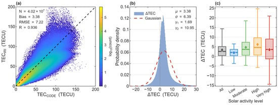
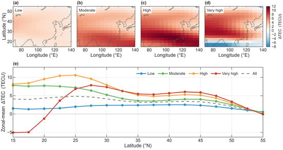
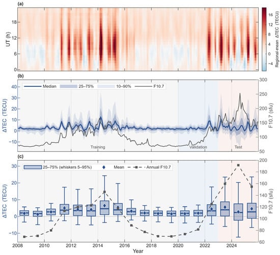
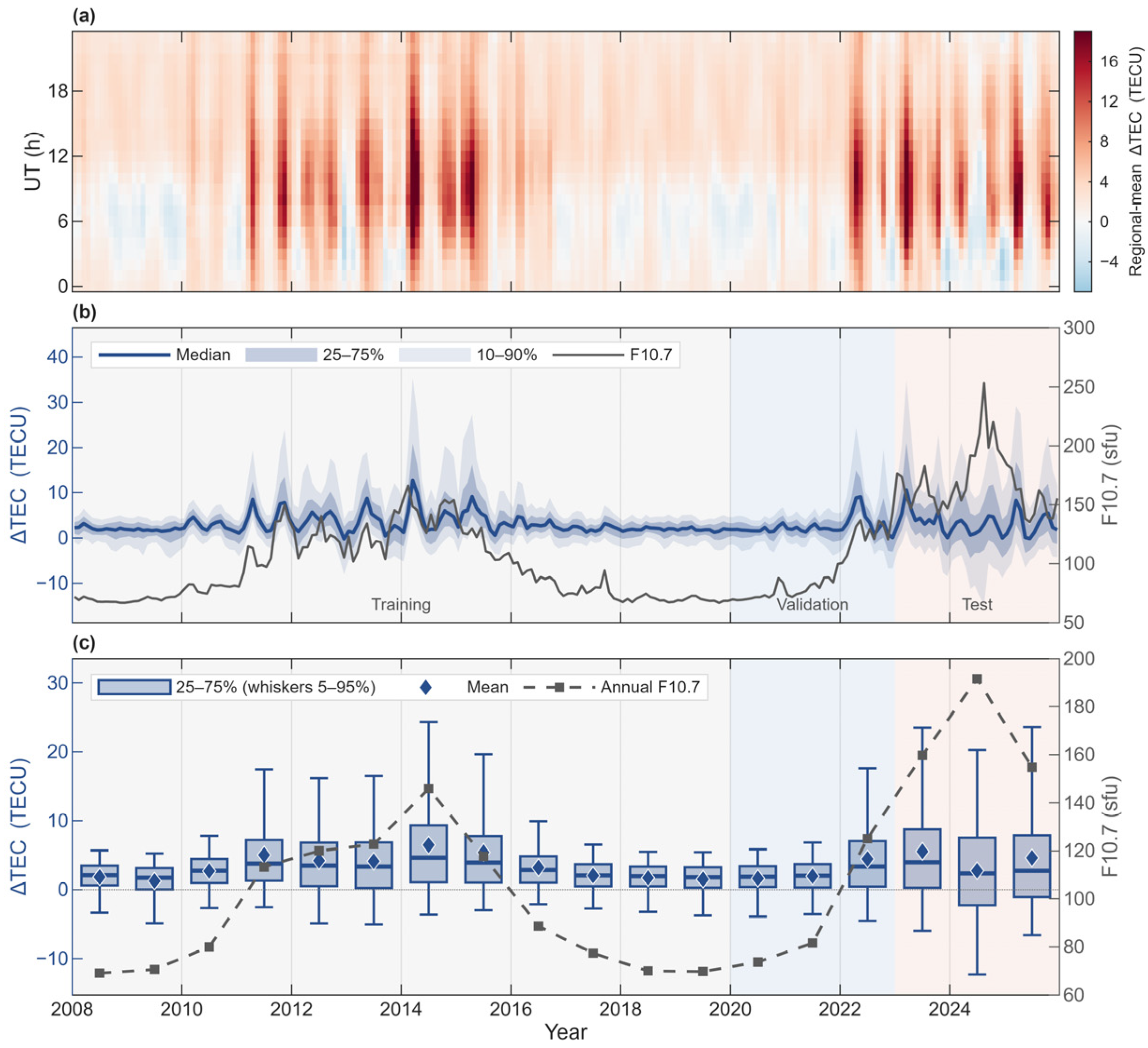
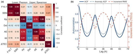
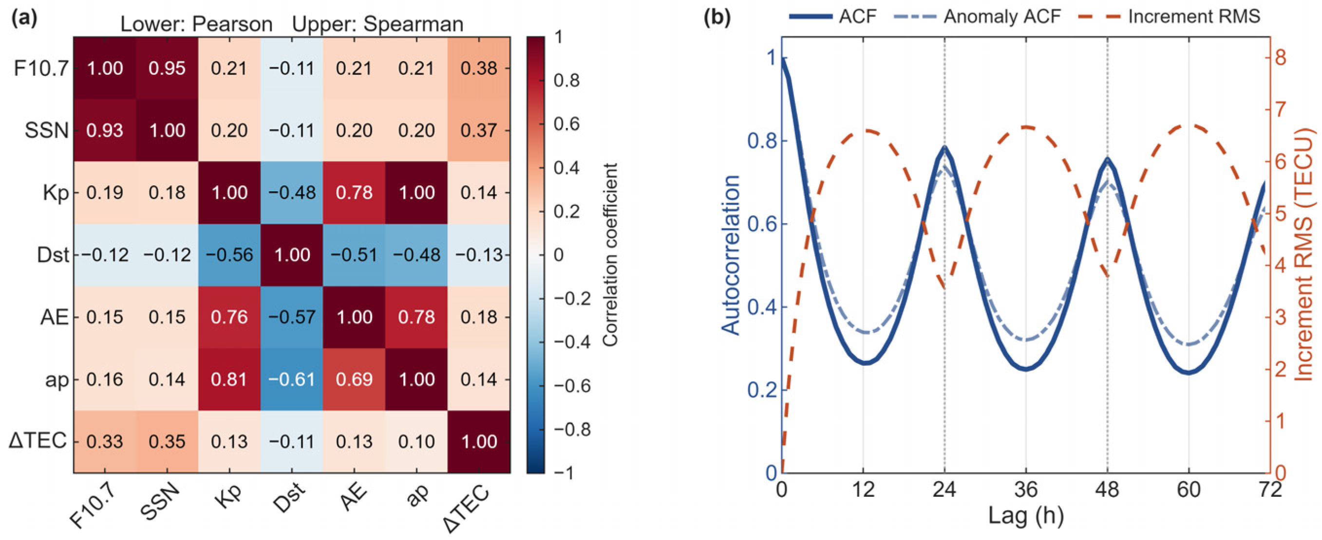
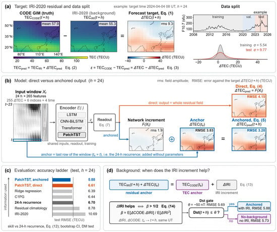
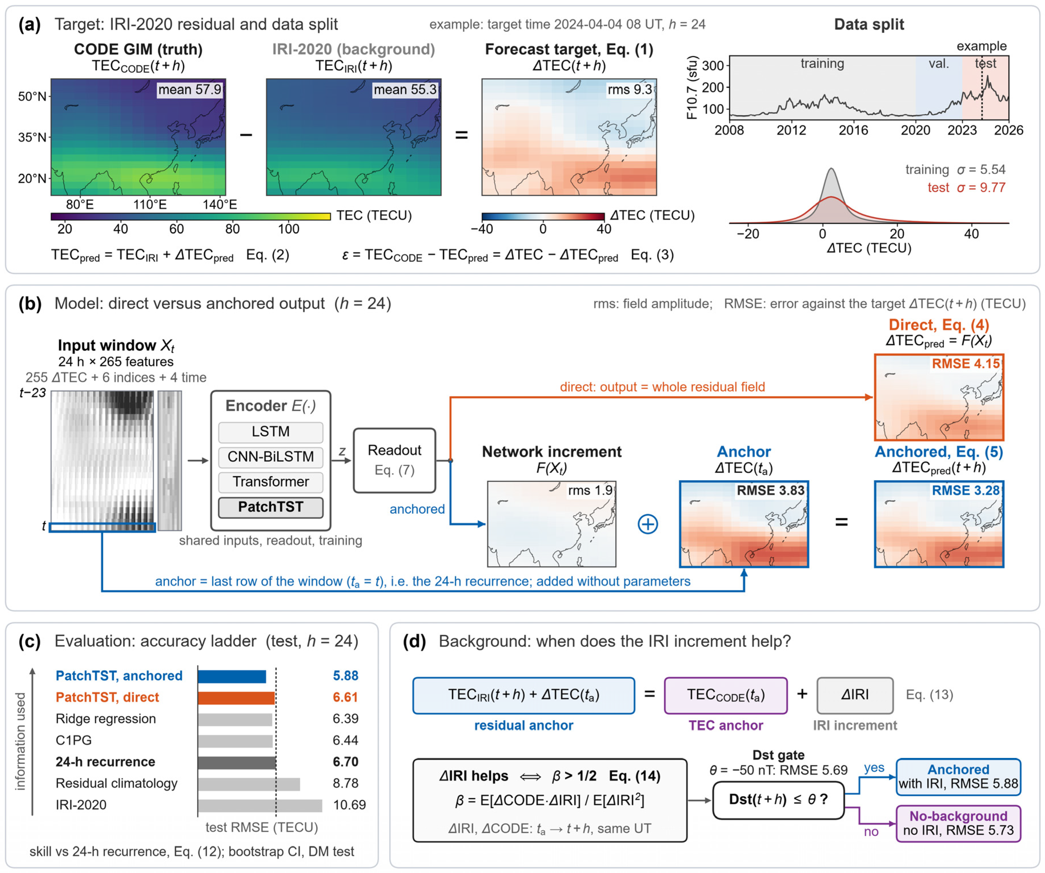
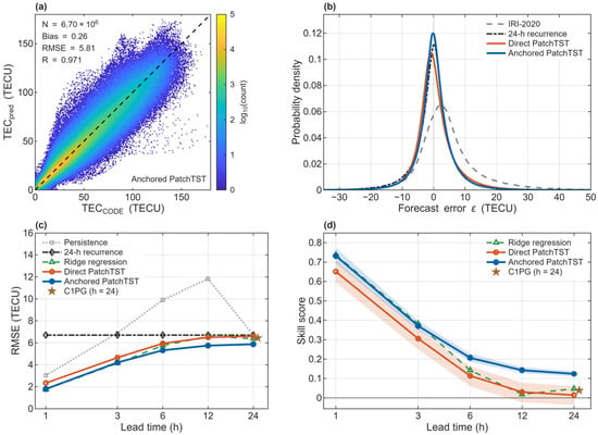
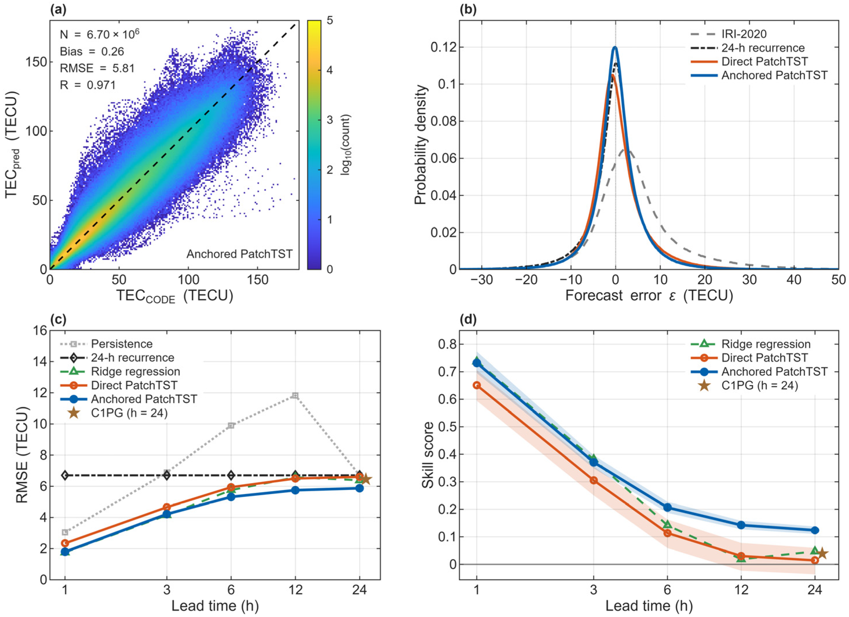
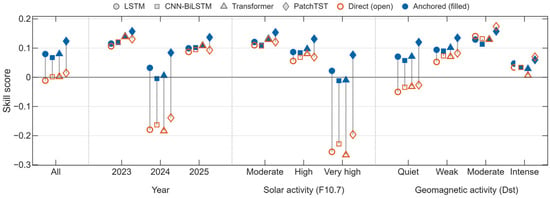
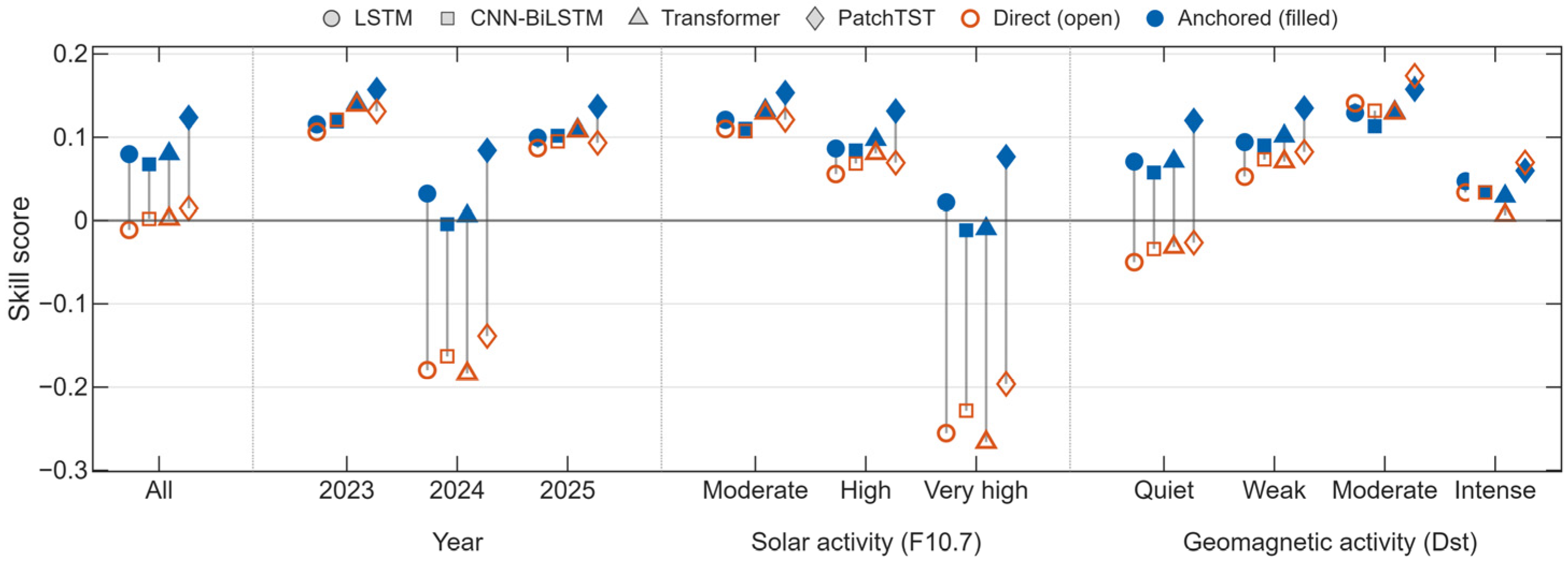
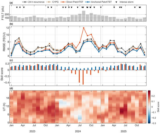
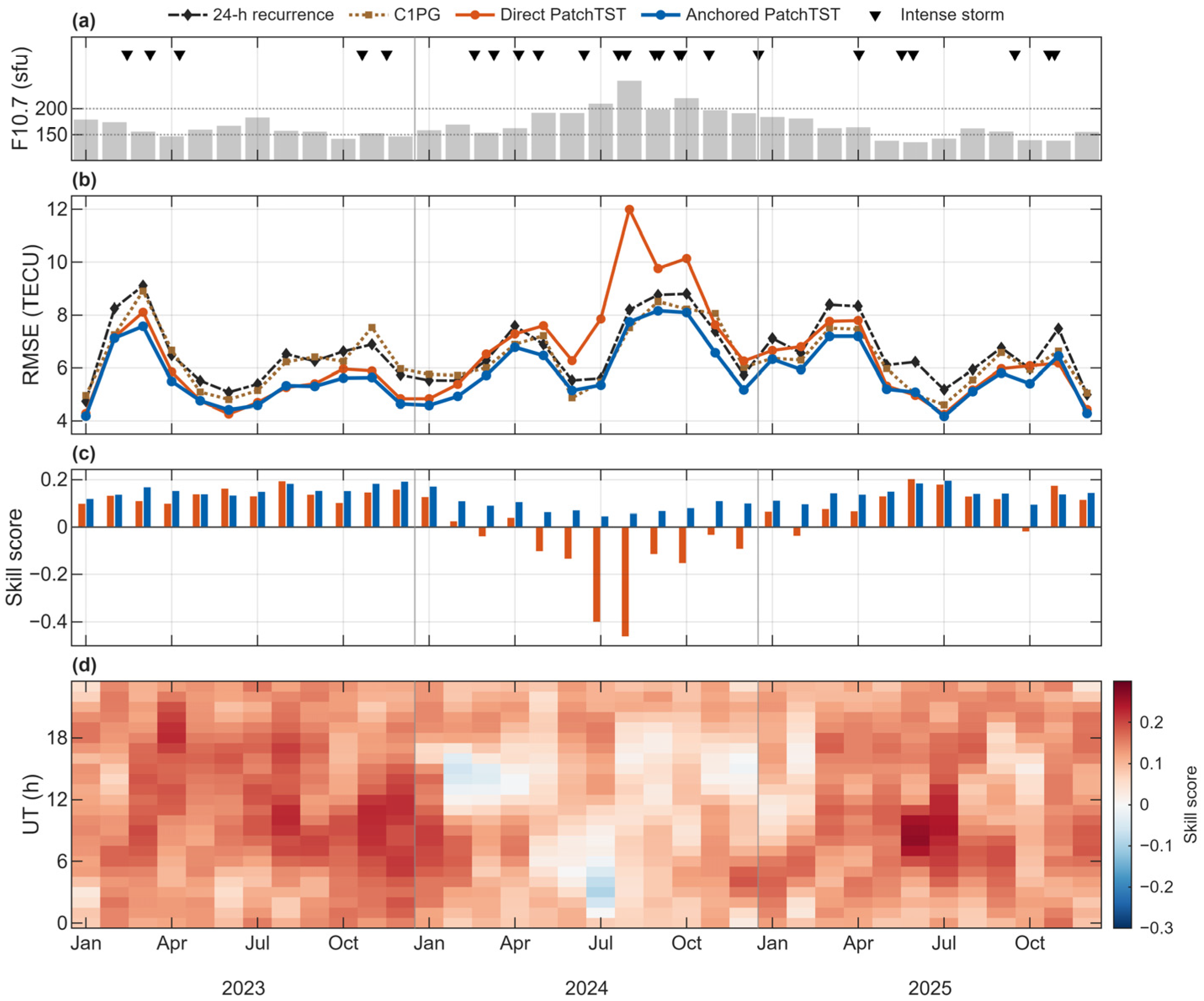
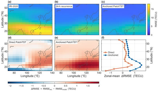
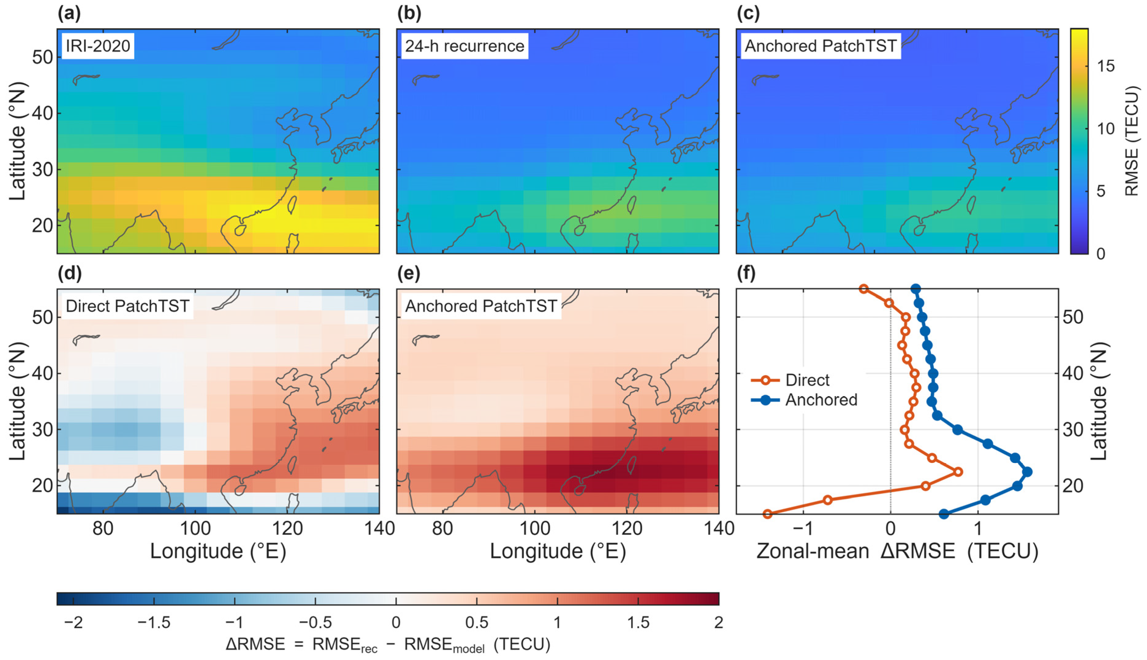
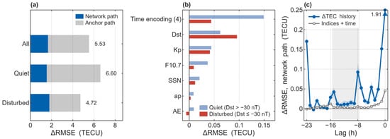
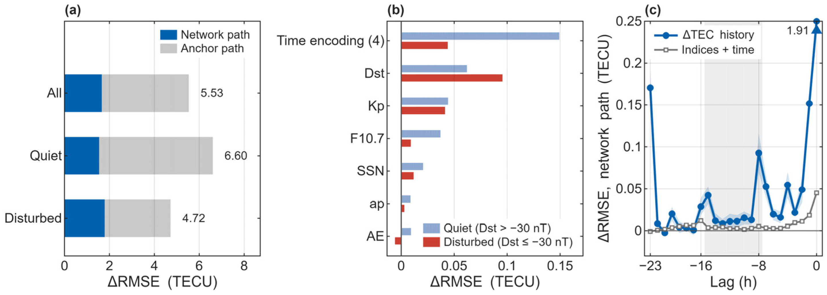
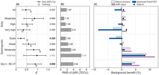
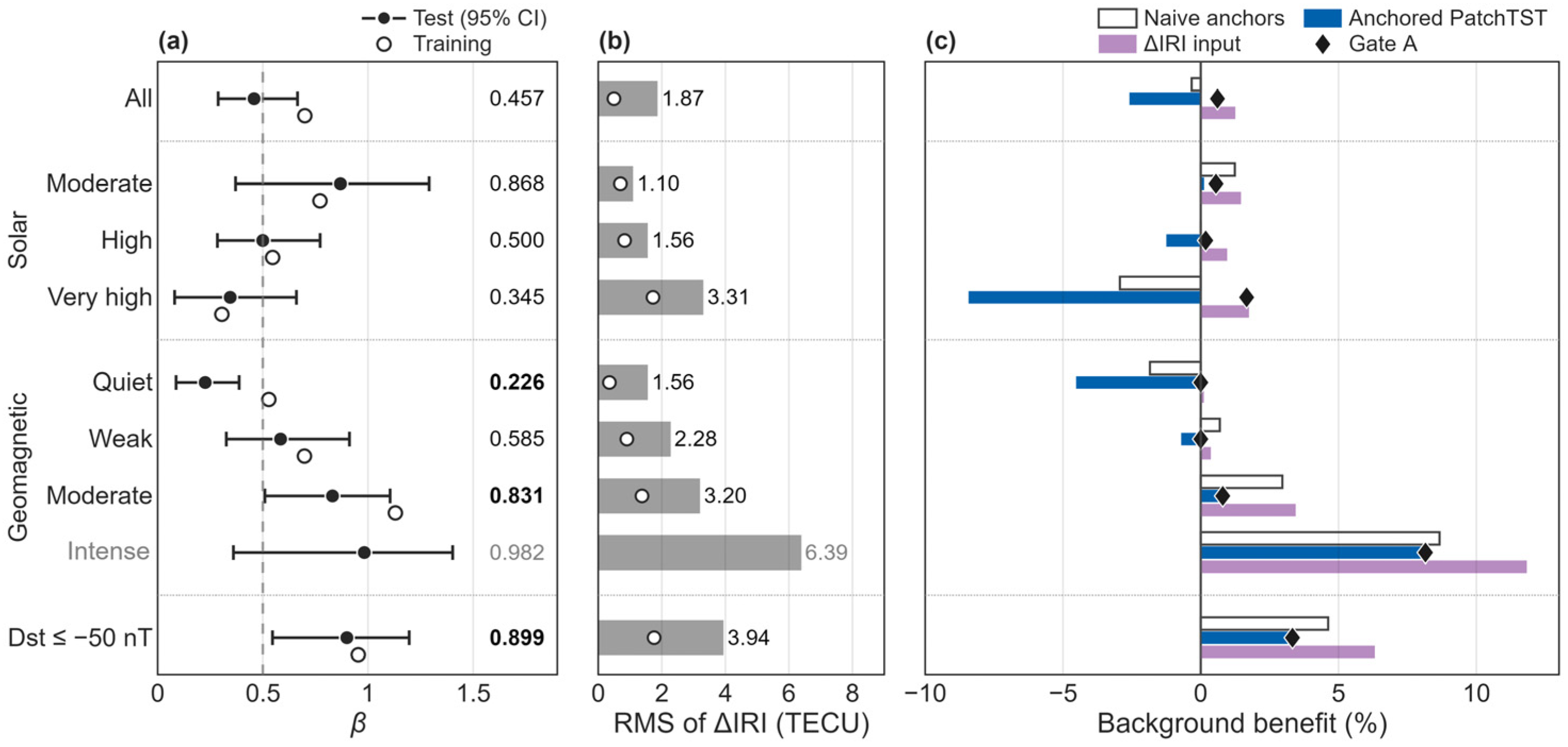
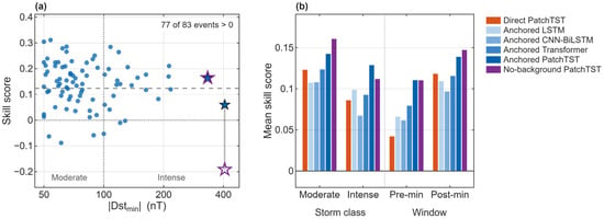
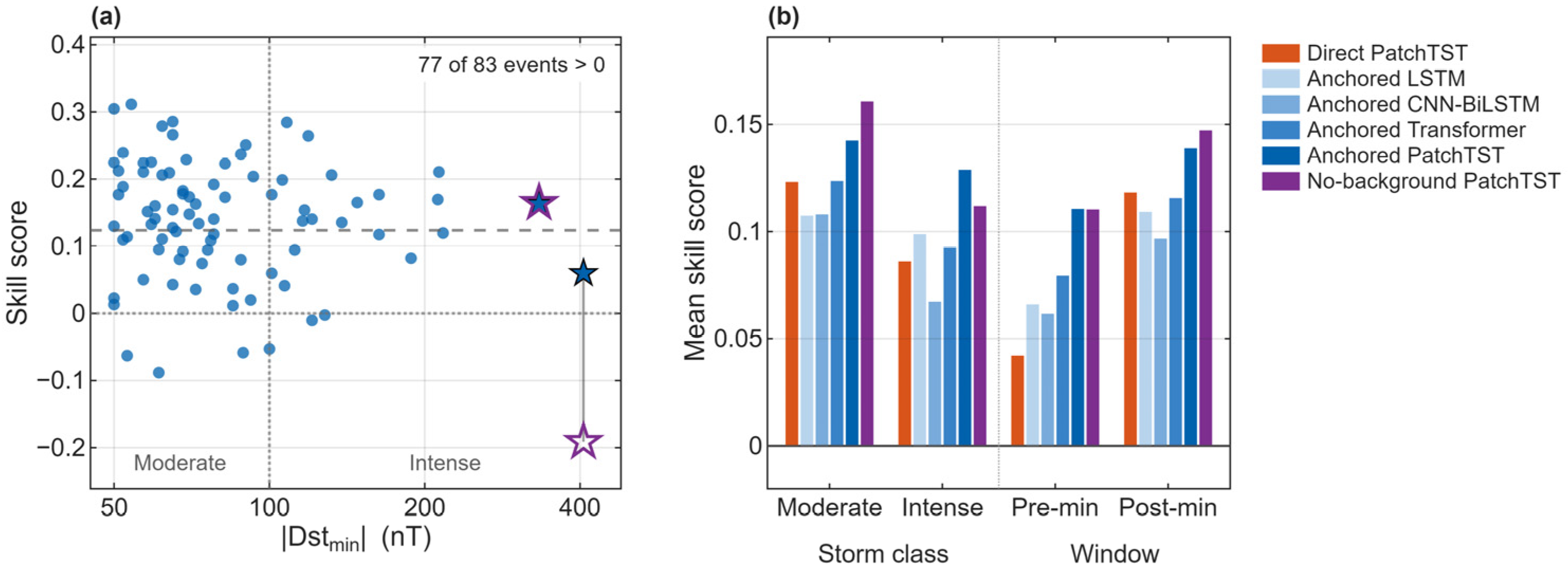
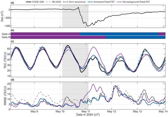
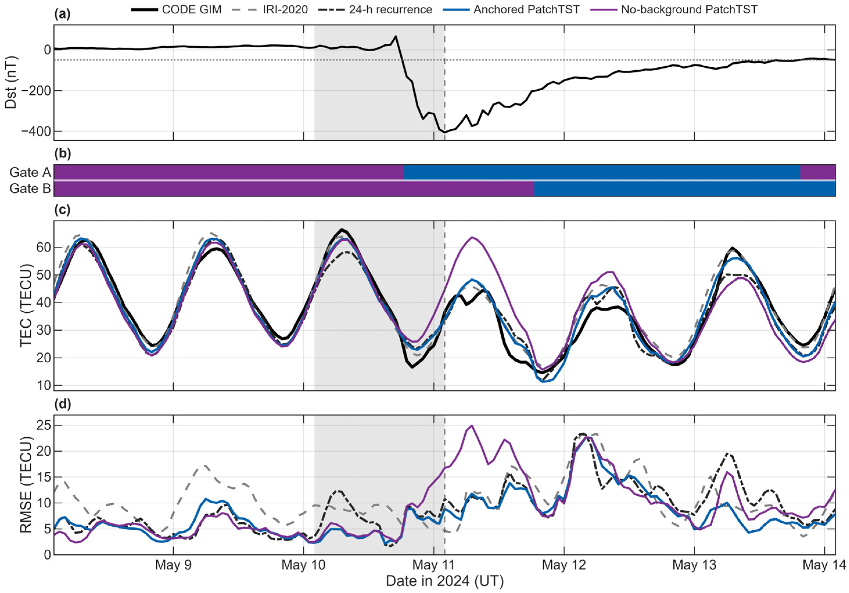
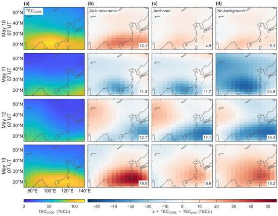
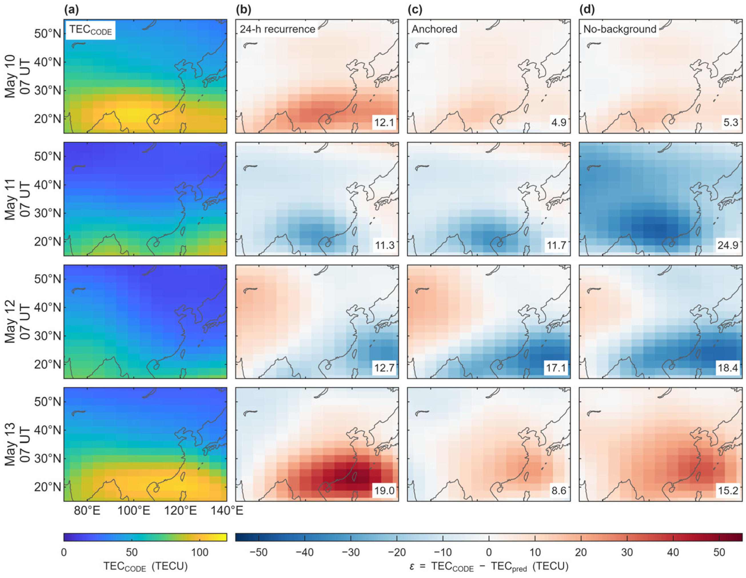

Disclaimer/Publisher’s Note: The statements, opinions and data contained in all publications are solely those of the individual author(s) and contributor(s) and not of MDPI and/or the editor(s). MDPI and/or the editor(s) disclaim responsibility for any injury to people or property resulting from any ideas, methods, instructions or products referred to in the content. |
© 2026 by the authors. Licensee MDPI, Basel, Switzerland. This article is an open access article distributed under the terms and conditions of the Creative Commons Attribution (CC BY) license.