Climatology of Spread Es over European Mid-Latitudes: Seasonal, Diurnal, and Spatial Variability During the Ascending Phase of Solar Cycle 25

Abstract

Spread sporadic-E (Spread-Es) appears in ionograms as diffuse and range-spread Es echoes associated with spatial structuring of the reflecting layer. In this study, five years (2020–2024) of Digisonde ionograms from three European mid-latitude stations—Juliusruh (54.6° N, 13.4° E), Dourbes (50.1° N, 4.6° E), and Roquetes (40.8° N, 0.5° E)—were visually inspected to investigate the seasonal, diurnal, and interannual variability of Spread-Es during the ascending phase of Solar Cycle 25. The Daily sunspot number is included only to provide solar-activity context for the 2020–2024 observational interval; no statistical assessment of solar-activity dependence is attempted. Spread-Es occurrence exhibited a pronounced summer and nighttime enhancement at all three stations. The normalised summer occurrence was 16.9% at Juliusruh, 8.6% at Dourbes, and 12.5% at Roquetes, compared with winter values of 5.6%, 2.6%, and 4.8%, respectively. The maximum monthly–hourly occurrence rates were approximately 0.48, 0.35, and 0.40, respectively, while Roquetes showed a broader post-midnight distribution. A representative multi-station interval on 12–13 June 2022 was further examined using ionograms, Height–Time–Intensity (HTI) representations, and regional detrended total electron content (dTEC) observations. Spread-Es and spread-F signatures coexisted at all three stations, with Spread-Es simultaneously present from 21:25 to 22:13 UT. The corresponding dTEC maps showed predominantly southwestward-propagating regional perturbations with NW–SE-oriented phase fronts. The derived phase speeds were 180–210 m s⁻¹, with periods of 48–64 min and horizontal wavelengths of approximately 518–806 km, characteristics consistent with nighttime MSTID activity over the European sector. Thus, the selected event shows the temporal coexistence of Spread-Es, spread-F, and regional MSTID-scale activity, while the available observations do not establish causal E–F electrodynamic coupling.

1. Introduction

The ionosphere is a highly dynamic region of the Earth’s upper atmosphere, extending from approximately 60 km to more than 1000 km in altitude. Within the E region (90–130 km), sporadic-E (Es) layers frequently occur as thin (typically <5 km), transient layers of enhanced ionisation that can persist from a few minutes to several hours [1,2]. These layers consist primarily of long-lived meteoric metallic ions, such as Fe⁺ and Mg⁺, and are formed through the combined effects of neutral-wind shear, ion–neutral collisions, and the geomagnetic field, commonly described by the wind-shear theory [1,2,3,4]. Once formed, Es layers can descend to lower altitudes, where atomic metallic ions are progressively converted through termolecular reactions into molecular ions that are subsequently removed by dissociative recombination [2]. Their occurrence and variability exhibit pronounced spatial, diurnal, and seasonal characteristics. At mid-latitudes, the strong summer maximum in Es occurrence and intensity has been related to the seasonal availability of meteoric metallic ions, while atmospheric tides and planetary waves contribute to the wind-shear dynamics controlling layer formation and variability [2,5].

Relationships between nighttime medium-scale travelling ionospheric disturbances MSTIDs and structured E-region plasma have been reported in previous mid-latitude observations. Otsuka et al. (2007) [6] simultaneously observed F-region MSTIDs in 630 nm airglow images and field-aligned irregularities in the E region, and found corresponding temporal behaviour between the MSTID and the E-region quasi-periodic echoes. Otsuka et al. (2008) [7] subsequently reported that nighttime MSTID activity was closely correlated with foEs and with foEs with the blanketing frequency of the sporadic-E layer (fbEs), defined as the maximum frequency below which echoes from higher ionospheric layers are obscured by the Es layer—with the latter representing spatial inhomogeneity of the Es plasma density—and discussed these results in terms of possible electrodynamic coupling between the Es layer and the F region. Spread-Es and spread-F have also been observed simultaneously under geomagnetically disturbed conditions. Wei et al. (2021) [8] reported simultaneous spread-F and intense Spread-Es during the recovery phase of the 7–9 September 2017 geomagnetic storm and suggested that the large-scale bottomside ionospheric tilts associated with these echoes might have been produced by large travelling ionospheric disturbances (LSTIDs). These studies therefore demonstrate observational relationships among E-region structuring, F-region disturbances, and travelling ionospheric disturbances, while the physical relationship among these phenomena may differ between individual events.

Atmospheric-wave forcing is a possible mechanism for generating additional structuring within an existing Es layer. Gravity waves can perturb the altitude and density distribution of Es and deform a horizontally stratified layer into tilted or wave-like structures. Chen et al. (2011) [9] showed that gravity-wave-induced deformation of an Es layer generated propagating wave-like plasma structures and off-vertical reflections manifested as Spread-Es. In their observations, variations in regular Es and in the Doppler velocity associated with Spread-Es exhibited a period of approximately 35 min, supporting atmospheric-wave modulation of the Es structure. Thus, gravity-wave forcing can contribute to the development of Spread-Es.

The causal link between structured Es layers and travelling ionospheric disturbances has been reported in past nighttime mid-latitude studies. Otsuka et al. (2007) [6] observed nighttime (MSTIDs) together with E-region field-aligned irregularities and reported coordinated E- and F-region disturbances. Otsuka et al. (2008) [7] subsequently established a link between nighttime MSTID occurrence and sporadic-E activity, including the spatial inhomogeneity of the Es layer. Simultaneous Spread-Es and spread-F have also been reported under disturbed conditions. Wei et al. (2021) [8], for example, observed Spread-Es and spread-F together with travelling ionospheric disturbances during the recovery phase of a geomagnetic storm. These studies show that structured Es and TID activity can coexist within the nighttime mid-latitude ionosphere, although they do not support MSTIDs as the only driver for Spread-Es.

Previous studies suggested an electrodynamic interaction between structured sporadic-E layers and the nighttime F region. Haldoupis et al. (2003) [10] proposed that polarisation electric fields generated within unstable and spatially structured sporadic-E layers can map along geomagnetic field lines to the F region and contribute to F-region plasma structuring and mid-latitude spread-F. Related theoretical studies have shown that sporadic-E and F-region instabilities can interact through polarisation electric fields and current closure in the nighttime mid-latitude ionosphere [11,12]. These mechanisms involve electrodynamic coupling between the E and F regions rather than physical transport of irregularities between the two regions. Therefore, they provide a possible physical explanation for some events in which structured Es and F-region disturbances occur simultaneously; however, the simultaneous appearance of E- and F-region ionogram signatures alone does not point to electrodynamic coupling.

In this study, we present a five-year climatological investigation of Spread-Es occurrence using ionograms from observations from three mid-latitude European Digisonde stations—Juliusruh, Dourbes, and Roquetes—during 2020–2024. We characterise the annual, seasonal, diurnal, and station-to-station spatial variability of Spread-Es and determine its occurrence percentage from the available ionograms. The stations were selected because they provide the most continuous ionogram records over 2020–2024; several other European stations had substantial data gaps during this period. The selected stations span 40.8° N–54.6° N and approximately 13° in longitude, allowing comparison across the European mid-latitude sector, although the three-station configuration does not constitute a dense latitudinal chain.

The temporal variation of daily Spread-Es duration is also compared with sunspot number during the study interval. In addition to the climatological analysis, a representative interval characterised by simultaneous Spread-Es and spread-F is examined using ionograms, Height–Time–Intensity (HTI) representations, and regional dTEC observations. The case study is used to characterise the temporal evolution of the ionospheric echoes and the regional ionospheric disturbance environment accompanying the Spread-Es/spread-F interval.

2. Materials and Methods

2.1. Digisonde Observations

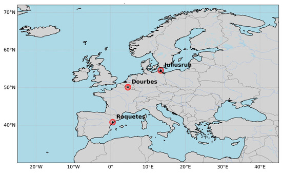
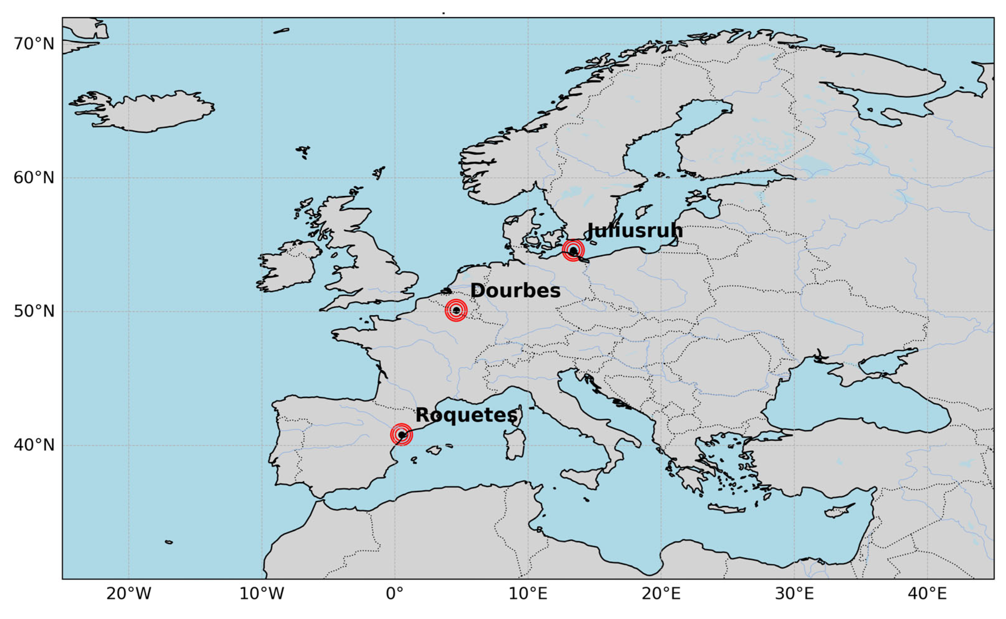
We analysed ionograms collected from three European mid-latitude Digisonde stations: Roquetes, Dourbes, and Juliusruh (Figure 1 and Table 1). The ionogram data were obtained from the Digital Ionogram Database (DIDBase) of the Global Ionospheric Radio Observatory (GIRO), Lowell GIRO Data Center (https://giro.uml.edu/didbase/ accessed on 15 January–22 March 2026). The GIRO network and DIDBase facilities are described by Reinisch and Galkin (2011) [13] and Khmyrov et al. (2008) [14], respectively. The observations considered in this study cover the period from January 2020 to December 2024 and were generally available at an approximately 5-min cadence, allowing the temporal evolution and persistence of Spread-Es to be tracked using consecutive ionograms.

Figure 1. Geographic locations of the three European mid-latitude Digisonde stations: Roquetes, Dourbes, and Juliusruh.

Table 1. Geographic and geomagnetic locations and nominal sampling cadence of the three European mid-latitude Digisonde stations.

Station	URSI Code	Geographic Coordinates	Geomagnetic Latitude	Cadence
Juliusruh	JR055	54.6° N, 13.4° E	52.6° N	~5 min
Dourbes	DB049	50.1° N, 4.6° E	47.2° N	~5 min
Roquetes	EB040	40.8° N, 0.5° E	36.1° N	~5 min

Ionogram availability was not uniform throughout the complete 2020–2024 interval. The principal periods of unavailable observations are summarised in Table 2. Only continuous data gaps longer than approximately 10 days are listed, although shorter interruptions were also present. Because the number of available ionograms varies among stations and time, all occurrence calculations were performed using only the corresponding available observations. Periods without ionograms were therefore not treated as periods without Spread-Es.

Table 2. Principal Digisonde data gaps during 2020–2024. Only continuous gaps longer than approximately 10 days are listed; missing intervals are given in day of year (DOY).

Station	Extended Data Gaps (Year: DOY)
Roquetes	2020: 284–294; 2021: 213–265; 2022: 351–365; 2023: 001–027, 035–113; 2024: 004–045, 047–067, 092–109
Dourbes	2020: 057–265; 2021: 247–258; 2024: 005–040
Juliusruh	2020: 057–093, 279–295; 2021: 247–258; 2023: 001–018; 2024: 001–060

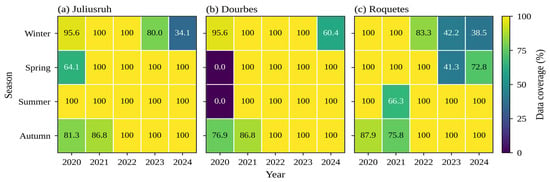
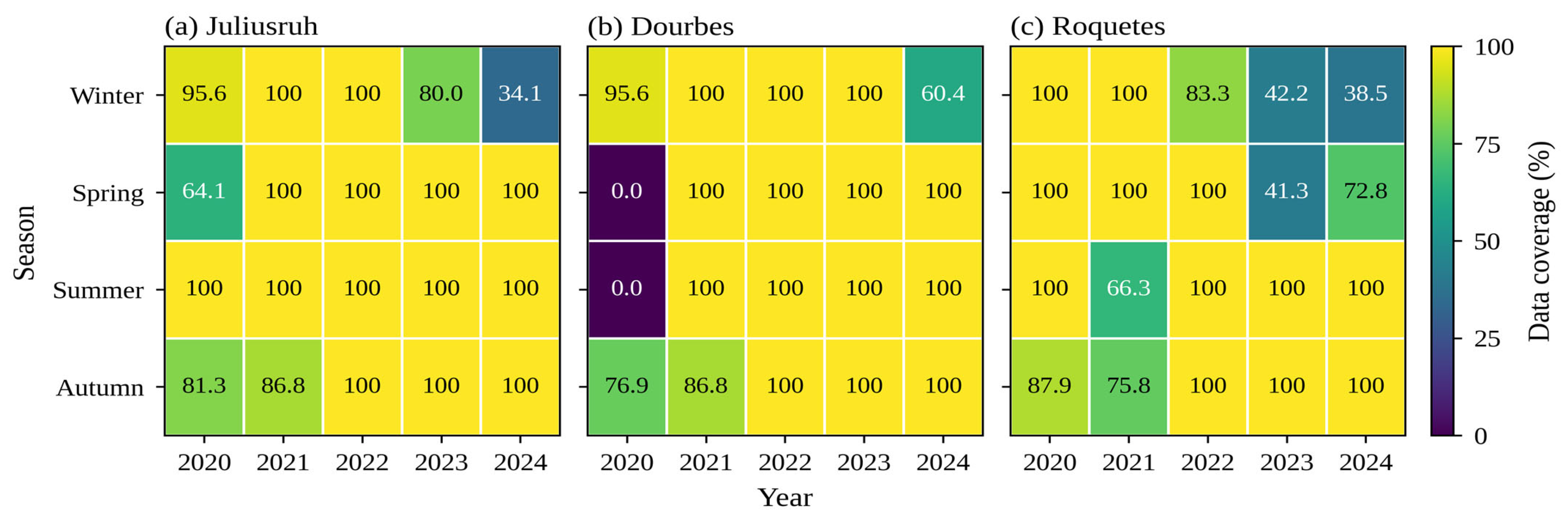
The data availability matrix (Figure 2) shows the percentage coverage for each station, year and season, calculated as the ratio of available to expected ionograms (288 per day at the 5-min sounding cadence).

Figure 2. Seasonal data coverage (%) of ionogram observations at (a) Juliusruh, (b) Dourbes and (c) Roquetes for 2020–2024, calculated as the ratio of available to expected ionograms (288 per day at a 5-min sounding cadence). Seasons are defined as winter (January, February, December), spring (March–May), summer (June–August) and autumn (September–November).

The matrix shows that the summer season, which is central to this study, is fully covered at all stations in all years except Dourbes in 2020, when no data were available, and Roquetes in 2021 (66.3% coverage). The large gaps at Roquetes in 2023–2024 and at Juliusruh in early 2024 fall mainly in winter and spring, when Spread-Es occurrence is low.

2.2. Identification of Spread-Es and Statistical Analysis

All available ionograms from the three stations were visually inspected to identify Spread-Es. The initial classification was performed through sequential visual examination of the ionograms, and the complete resulting catalogue was subsequently rechecked against the original ionograms by a second observer before being used for the statistical analysis. Ambiguous classifications identified during this verification stage were re-examined before the final catalogue was established. The classification was therefore based on a two-stage manual inspection and verification procedure; no automated classification algorithm or software-based threshold was used to identify Spread-Es.

Manual visual interpretation remains an established approach for the identification of complex ionogram morphologies. The interpretation of ionogram and sporadic-E trace morphology followed the general conventions of the URSI Handbook of Ionogram Interpretation and Reduction [15,16]. Previous studies dealing with diffuse or spread-like sporadic-E signatures have likewise relied on visual examination of ionograms. Zhou et al. (2018) [17], for example, examined diffuse-Es signatures in Digisonde observations using visual verification, while Moro et al. (2025) [18] visually inspected approximately 83,000 Digisonde ionograms to identify and statistically characterize height-spread Es signatures.

For the present study, Spread-Es was identified as diffuse or broadened Es echoes exhibiting appreciable spreading in virtual range compared with the comparatively narrow trace of a regular Es layer. The ionograms were examined sequentially, and Spread-Es was considered valid when the characteristic spreading was present in at least three consecutive ionograms. At the nominal sampling cadence of approximately 5 min, three consecutive observations span approximately 10 min from the first to the third sounding. This persistence criterion was adopted as a conservative measure to reduce the inclusion of isolated noise, transient trace distortions, interference, or ambiguous spreading. Consequently, genuine Spread-Es signatures persisting for fewer than three consecutive observations were not included in the statistical catalogue. The reported occurrence rates therefore represent persistent, visually identifiable Spread-Es under the adopted criterion rather than an inventory of every short-lived Spread-Es signature.

The observers were not blinded to station or observation time because the ionograms were examined sequentially in order to evaluate the temporal persistence of the signatures. Station and date, however, were not themselves used as classification criteria; identification was based on the observed ionogram morphology and its persistence in consecutive soundings. Because the second-stage assessment consisted of a complete verification and reconciliation of the catalogue rather than a parallel independent classification retained as a separate dataset, a formal inter-observer agreement statistic such as Cohen’s κ was not calculated.

A total of 1,275,650 available ionograms were inspected during 2020–2024, comprising 475,648 at Juliusruh, 384,306 at Dourbes, and 415,696 at Roquetes. The initial visual catalogue contained 69,316 Spread-Es ionograms. After application of the strict three-consecutive-ionogram criterion, 64,175 Spread-Es ionograms were retained, comprising 24,960 at Juliusruh, 10,981 at Dourbes, and 28,234 at Roquetes (Table 3).

Table 3. Numbers of available and Spread-Es ionograms at Juliusruh, Dourbes and Roquetes during 2020–2024.

Station	Available Ionograms	Spread-Es Ionograms (As Classified)	Fraction (%)	Spread-Es Ionograms (Strict Rule)	Fraction (%)
Juliusruh	475,648	25,346	5.33	24,960	5.25
Dourbes	384,306	15,266	3.97	10,981	2.86
Roquetes	415,696	28,704	6.91	28,234	6.79
Total	1,275,650	69,316	5.43	64,175	5.03

Note: “As classified” gives the number of ionograms identified as Spread-Es in the catalogue; “strict rule” gives the number remaining when Spread-Es is counted only in sequences of at least three consecutive soundings at the nominal 5-min cadence. Fractions are calculated as the ratio of Spread-Es ionograms to available ionograms (Equations (1) and (2)); missing soundings are excluded from both.

Because data availability varied among stations and with time, the Spread-Es occurrence rate within each analysis bin was calculated from the available ionograms as

$${\mathrm{R}}_{\mathrm{S}\mathrm{p}\mathrm{r}\mathrm{e}\mathrm{a}\mathrm{d}-\mathrm{E}\mathrm{s}}={\displaystyle \frac{{\mathrm{N}}_{\mathrm{S}\mathrm{p}\mathrm{r}\mathrm{e}\mathrm{a}\mathrm{d}-\mathrm{E}\mathrm{s}}}{{\mathrm{N}}_{\mathrm{T}\mathrm{o}\mathrm{t}\mathrm{a}\mathrm{l}}}}$$

(1)

where N_Spread-Es is the number of available ionograms containing validated Spread-Es within the corresponding analysis bin, and N_Total is the total number of available ionograms within the same bin. When expressed as a percentage,

$${\mathrm{P}}_{\mathrm{S}\mathrm{p}\mathrm{r}\mathrm{e}\mathrm{a}\mathrm{d}-\mathrm{E}\mathrm{s}}=100\times {\displaystyle \frac{{\mathrm{N}}_{\mathrm{S}\mathrm{p}\mathrm{r}\mathrm{e}\mathrm{a}\mathrm{d}-\mathrm{E}\mathrm{s}}}{{\mathrm{N}}_{\mathrm{T}\mathrm{o}\mathrm{t}\mathrm{a}\mathrm{l}}}}$$

(2)

Thus, the calculated occurrence rate represents the fraction of available ionograms exhibiting Spread-Es rather than the number of independent Spread-Es events.

The temporal distribution of Spread-Es was first examined as a function of day of year (DOY) and universal time (UT) for each station and year during 2020–2024. Seasonal comparisons were performed using winter (November–February), equinox (March–April and September–October), and summer (May–August). For the monthly-diurnal analysis, the available ionograms were grouped into 1-h UT bins, and the occurrence rate within each month-hour bin was calculated using Equation (1). Sunrise and sunset curves were superimposed on the plots to provide a solar-terminator reference.

To examine the day-to-day variation of Spread-Es, the cumulative daily Spread-Es duration was estimated from the number of available ionograms containing validated Spread-Es:

$${\mathrm{D}}_{\mathrm{S}\mathrm{p}\mathrm{r}\mathrm{e}\mathrm{a}\mathrm{d}-\mathrm{E}\mathrm{s}}={\displaystyle \frac{{\mathrm{N}}_{\mathrm{S}\mathrm{p}\mathrm{r}\mathrm{e}\mathrm{a}\mathrm{d}-\mathrm{E}\mathrm{s},\mathrm{d}\mathrm{a}\mathrm{y}}\mathsf{\Delta }\mathrm{t}}{60}}$$

(3)

where D_Spread-Es is the cumulative daily Spread-Es duration in hours, N_{Spread-Es,day} is the number of available ionograms containing validated Spread-Es within the corresponding UT day, and Δt is the nominal Digisonde sampling interval in minutes, taken as approximately 5 min in the present analysis. Intervals without available ionogram observations were not included in the calculation. Because Equation (3) converts the number of classified ionograms into cumulative sampled time, it should not be interpreted as the duration of a single continuous Spread-Es event when multiple separated Spread-Es intervals occur within the same day.

2.3. Sunspot Number Data

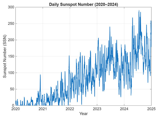
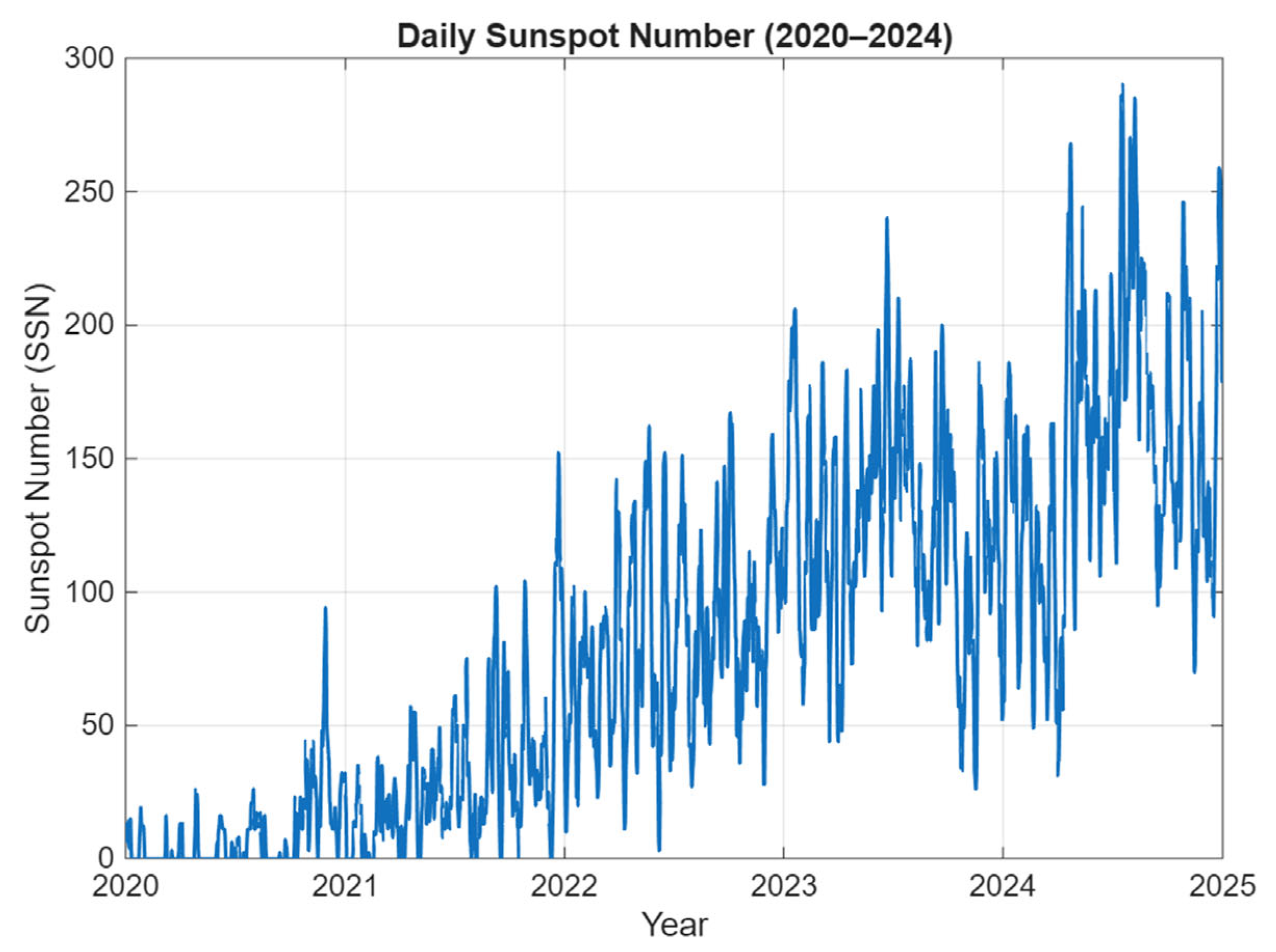
Daily sunspot number (SSN) was used only to provide the solar-activity context for the 2020–2024 observational interval. The daily SSN data were obtained from the NASA Goddard Space Flight Center OMNIWeb database (https://omniweb.gsfc.nasa.gov/form/dx1.html, accessed on 10 April 2026). The SSN series illustrates the progression of solar activity during the ascending phase of Solar Cycle 25 (Figure 3). Because Spread-Es occurrence exhibits strong seasonal and local-time dependence, while observational coverage also varies among stations and years, no correlation or statistical inference between SSN and Spread-Es occurrence or duration was performed. A quantitative assessment of solar-activity dependence would require seasonally and local-time controlled occurrence measures, appropriate treatment of observational coverage, and preferably observations spanning a longer portion of the solar cycle. The SSN observations are therefore used only as contextual information in the present study.

Figure 3. Daily sunspot number from January 2020 to December 2024, illustrating the progression of solar activity during the ascending phase of Solar Cycle 25.

2.4. Height–Time–Intensity Analysis

The temporal development of ionospheric echoes during the selected event was further examined using Height–Time–Intensity (HTI) plots from consecutive ionograms following the methodology described by Haldoupis et al. (2006) [19]. For each sounding, the echo intensity was mapped as a function of virtual height, and the resulting profiles were arranged chronologically to form a two-dimensional representation, with universal time along the horizontal axis and virtual height along the vertical axis.

Only echoes recorded within the 2–10 MHz sounding-frequency range were considered. This frequency interval was selected to reduce contributions from low-frequency noise while retaining the principal ionospheric echoes. Compared with inspection of individual ionograms, the HTI plot is representative of changes in virtual height, persistence, and temporal evolution of the echo at the typical 5-min Digisonde cadence. The HTI displays virtual height variations and not true height.

2.5. GNSS dTEC Observations and TID Characterisation

Regional ionospheric perturbations associated with the selected event were examined using detrended Total Electron Content (dTEC) observations obtained from the Global GNSS-TEC database maintained by the Institute for Space–Earth Environmental Research (ISEE), Nagoya University. The gridded dTEC data were downloaded from the GRID2 NetCDF archive (https://stdb2.isee.nagoya-u.ac.jp/GPS/GPS-TEC/ accessed on 1–2 April 2026). The GNSS TEC mapping technique used to generate the gridded observations is described by Otsuka et al. (2002) [20], while the application of regional TEC observations to the investigation of travelling ionospheric disturbances over Europe is described by Otsuka et al. (2013) [21].

For the present analysis, the geographical domain was restricted to 30–70° N latitude and 10° W–36° E longitude, encompassing the three Digisonde stations and the surrounding European sector. The dTEC observations were examined at 5-min intervals using the native 0.25° × 0.25° geographic latitude–longitude grid of the GRID2 product. A common display range of −0.4 to +0.4 TECU was applied to successive maps to allow direct visual comparison of the positive and negative perturbation structures. Values exceeding these limits were saturated only for visualisation, while the underlying dTEC values remained unchanged.

The identification and quantitative characterisation of the propagating dTEC disturbance followed the methodology described in detail by Paul et al. (2026) [22]. Successive dTEC maps were first examined to identify spatially coherent positive and negative perturbation structures exhibiting systematic horizontal progression through consecutive epochs. An isolated enhancement or depletion was not regarded as evidence of a propagating disturbance unless the perturbation retained a coherent wave-like morphology and showed consistent phase progression through time.

For the quantitative analysis, the dTEC time series at the GRID2 point nearest each Digisonde was used to determine the dominant oscillation period. After removal of the temporal mean over the selected event interval, a Fast Fourier Transform (FFT) was applied, and the positive-frequency spectral component with the largest amplitude was used to estimate the dominant period, following Paul et al. (2026) [22]. The propagation direction was determined independently from the systematic spatial progression of coherent dTEC phase fronts through successive map epochs, with the propagation vector taken approximately normal to the phase-front orientation.

Horizontal propagation speed was estimated from the displacement of the coherent disturbance through consecutive epochs using the geographic positions of the tracked disturbance and surface geodesic distances, following Paul et al. (2026) [22]. If P_k denotes the geographic position of the tracked disturbance at epoch t_k, the accumulated geodesic displacement between consecutive valid positions was divided by the elapsed time between the first and last retained epochs to obtain the representative horizontal propagation speed. The horizontal wavelength was subsequently estimated from the characteristic propagation speed and dominant period. The complete mathematical formulation and implementation details are given by Paul et al. (2026) [22].

For the present event, the Europe-wide maps were used for visualisation of the regional disturbance, whereas quantitative parameter estimation was performed within a local station-centred analysis region following the procedure of Paul et al. (2026) [22]. This distinction prevents the large display domain from being interpreted as the spatial window used for the parameter calculation. Parameter uncertainties were treated as event-dependent rather than assigned fixed values. They depend on the 0.25° × 0.25° GRID2 sampling, source-product spatial smoothing, the temporal sampling and finite duration of the event interval, and uncertainty in localising the same coherent disturbance through successive epochs. In particular, the spectral resolution of the dominant period depends on the duration of the available dTEC time series, so a single fixed period uncertainty is not appropriate. Likewise, the uncertainty of the propagation-speed estimate depends on both spatial localisation and elapsed tracking time. These limitations were taken into account when reporting and interpreting the derived MSTID parameters.

The dTEC analysis was applied only to the representative event examined in Section 3.5 and was not used to infer TID or MSTID occurrence throughout the complete five-year Spread-Es climatology. The Digisonde observations therefore provide the long-term Spread-Es statistics, whereas the HTI and dTEC observations provide complementary information on the propagation of ionospheric disturbance during the selected event.

3. Results

3.1. Representative Spread-Es Morphology

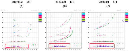
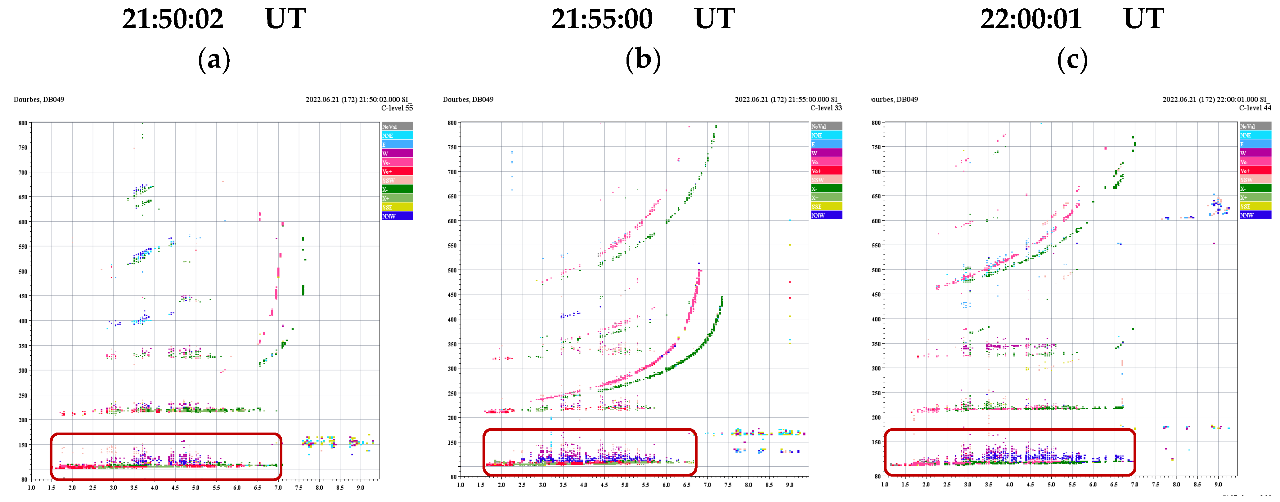
Figure 3 shows three representative Spread-Es ionograms observed at Dourbes on 21 June 2022. In Figure 4a, recorded at 21:50:02 UT, the main Es reflection appears near a virtual height of approximately 100–110 km, while diffuse echoes extend above the principal trace to a virtual height of about 150 km. Within this spread region, several colour-coded off-vertical echoes are also visible. In the DPS-4D ionograms, the colour coding represents the horizontal direction of arrival of the received echoes. Non-vertical echoes are grouped into the directional sectors NNE, E, SSE, SSW, W, and NNW; therefore, the different colours indicate echoes arriving from different horizontal directions rather than differences in echo intensity. Echoes associated with the W direction are particularly evident above the main Es trace, together with weaker echoes from other directions, including the NNE, NNW, and SSW sectors. In Figure 4b, recorded at 21:55:00 UT, the spreading becomes more pronounced, and the diffuse echoes extend to approximately 160 km virtual height. The off-vertical echoes are also more clearly developed, with W-directed echoes forming a substantial part of the spread structure and additional echoes visible from the NNE, NNW, and SSW directions. In Figure 4c, recorded at 22:00:01 UT, the Spread-Es remains clearly visible and extends to approximately 170 km virtual height. At this time, the spread region contains a broader mixture of colour-coded echoes, with prominent W-directed echoes and additional NNE-, NNW-, and other directionally separated echoes. Thus, the sequence demonstrates not only the persistence and increasing virtual-range extent of the diffuse Es echoes over consecutive ionograms, but also the presence of off-vertical echoes arriving from several directions, which contribute to the observed Spread-Es morphology.

Figure 4. Representative Spread-Es ionograms observed at Dourbes on 21 June 2022: (a) 21:50:02 UT, (b) 21:55:00 UT, and (c) 22:00:01 UT. The red boxes indicate the Spread-Es. In all three ionograms, the main Es reflection is located near 100–110 km virtual height, while diffuse echoes extend to higher virtual ranges, illustrating the characteristic spreading used for the manual identification of Spread-Es. The different colours of the echoes indicate their horizontal directions of arrival.

The extended echoes in Figure 4 represent virtual-height spreading and should not be interpreted as the true physical thickness of the Es layer. Spatially structured, tilted, or horizontally inhomogeneous Es layers can produce multiple and off-vertical propagation paths, which appear in ionograms as diffuse or range-spread echoes. Barnes (1992) [23] showed that structured Spread-Es can generate multiple refracted propagation paths, while Chen et al. (2011) [9] demonstrated that deformation and tilting of an Es layer can produce off-vertical reflections appearing as Spread-Es. The sequence presented in Figure 4 therefore illustrates the morphology used for the manual identification of Spread-Es in the present analysis.

3.2. Annual and Seasonal Distribution of Spread-Es

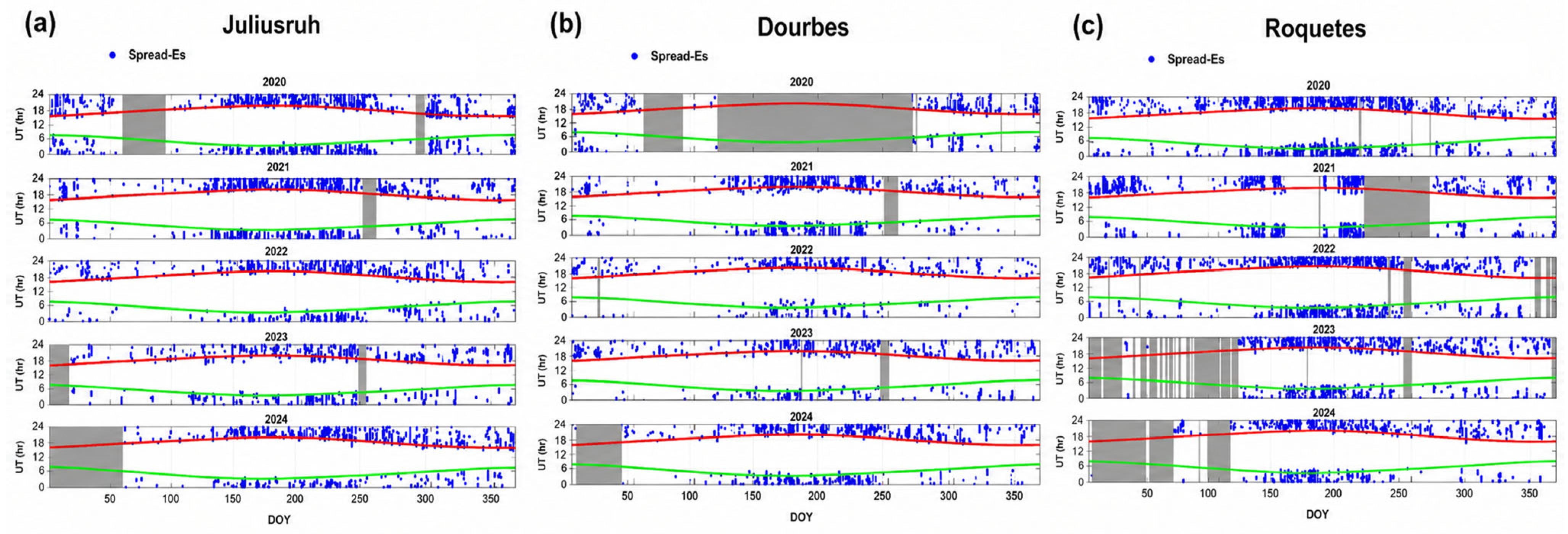
Figure 5 presents the temporal distribution of Spread-Es observations at Juliusruh, Dourbes, and Roquetes during 2020–2024 as a function of day of year (DOY) and universal time (UT). The blue markers represent ionograms containing Spread-Es, while the grey-shaded intervals indicate periods of unavailable observations. The green and red curves represent sunrise and sunset, respectively. The principal data gaps are summarised in Table 2. For the seasonal analysis, winter is defined as November–February, equinox as March–April and September–October, and summer as May–August. All three stations show a higher Spread-Es occurrence during summer nighttime.

Figure 5. Temporal distribution of Spread-Es observations at (a) Juliusruh, (b) Dourbes, and (c) Roquetes during 2020–2024. Blue markers represent Spread-Es ionograms. Green and red curves indicate sunrise and sunset, respectively, while grey-shaded intervals denote periods of unavailable Digisonde observations. The horizontal axis represents day of year (DOY), and the vertical axis represents universal time (UT). The principal extended data gaps are summarised in Table 2.

At Juliusruh (Figure 5a), Spread-Es are observed in all five years, with increased occurrence generally extending from late spring through summer. The summer nighttime peak is clearly visible, although Spread-Es are also sporadically observed during the whole year. There are some data gaps, particularly during 2020, 2023, and at the beginning of 2024.

At Dourbes (Figure 5b), Spread-Es also shows a clear summer nighttime enhancement. Interpretation of the yearly distributions requires caution because of the extended data gaps, particularly during 2020 when a substantial part of the spring–summer interval is unavailable. During 2021–2024, the available observations show a clearer summer enhancement, with fewer Spread-Es observations during the other seasons.

At Roquetes (Figure 5c), Spread-Es is again observed mainly during summer, with the nighttime occurrence extending over a relatively broad interval. The yearly distributions are affected by data gaps, particularly during 2021, 2023, and 2024.

The seasonal comparison therefore shows a consistent summer enhancement at all three stations. The highest summer occurrence is observed at Juliusruh (16.9%), followed by Roquetes (12.5%) and Dourbes (8.6%), while the corresponding winter values are 5.6%, 4.8%, and 2.6%, respectively. The differences between the stations should be considered together with the corresponding observational coverage.

3.3. Monthly–Hourly Spread-Es Occurrence Rate

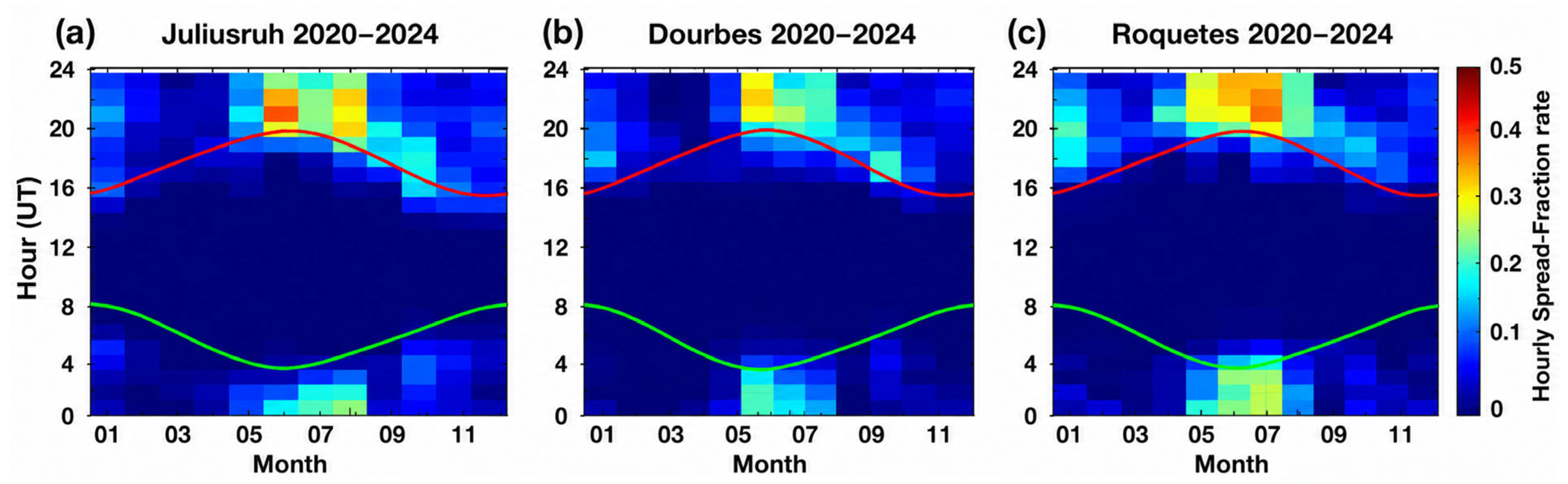
Figure 6 presents the monthly–hourly Spread-Es occurrence rate over Juliusruh, Dourbes, and Roquetes using all available observations during 2020–2024. The occurrence rate in each month–hour bin was calculated from the corresponding number of available ionograms, as described in Section 2.2. The green and red curves indicate sunrise and sunset, respectively.

Figure 6. Monthly–hourly Spread-Es occurrence rate at (a) Juliusruh, (b) Dourbes, and (c) Roquetes during 2020–2024. The horizontal axis represents month, and the vertical axis represents universal time (UT). The colour scale indicates the fraction of Spread-Es ionograms within each 1-h month–UT bin. Green and red curves indicate sunrise and sunset, respectively.

At Juliusruh (Figure 6a), the highest occurrence rates are observed during summer, particularly from June to August. The main enhancement occurs during nighttime hours, with the highest values around 20:00–22:00 UT. Increased occurrence extends across midnight into early-morning hours, particularly during June–August. A weaker enhancement is visible during winter, mainly in the evening and early-morning hours. The maximum hourly occurrence rate is approximately 0.48.

At Dourbes (Figure 6b), a similar summer nighttime enhancement is observed, with the highest values mainly during June and July between approximately 20:00 and 23:00 UT. Spread-Es occurrence also extends into the post-midnight hours. A weaker wintertime occurrence is visible, particularly during December–January. The maximum hourly occurrence rate is approximately 0.35.

At Roquetes (Figure 6c), the enhanced nighttime occurrence extends over a broader seasonal and temporal interval. Increased occurrence is observed from approximately May to August, with the highest values during June–July. Compared with Juliusruh and Dourbes, the enhanced occurrence extends farther through the nighttime hours, from evening to approximately 03:00 UT. The maximum hourly occurrence rate is approximately 0.40. A weaker wintertime enhancement is also observed during nighttime.

Overall, Juliusruh shows the highest maximum hourly occurrence rate (0.48), followed by Roquetes (0.40) and Dourbes (0.35), while Roquetes shows a broader summer nighttime distribution. These results show differences in the magnitude and temporal distribution of Spread-Es occurrence among the three stations.

3.4. Solar-Activity Context During 2020–2024

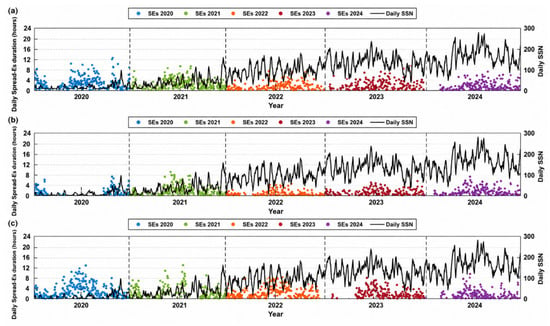
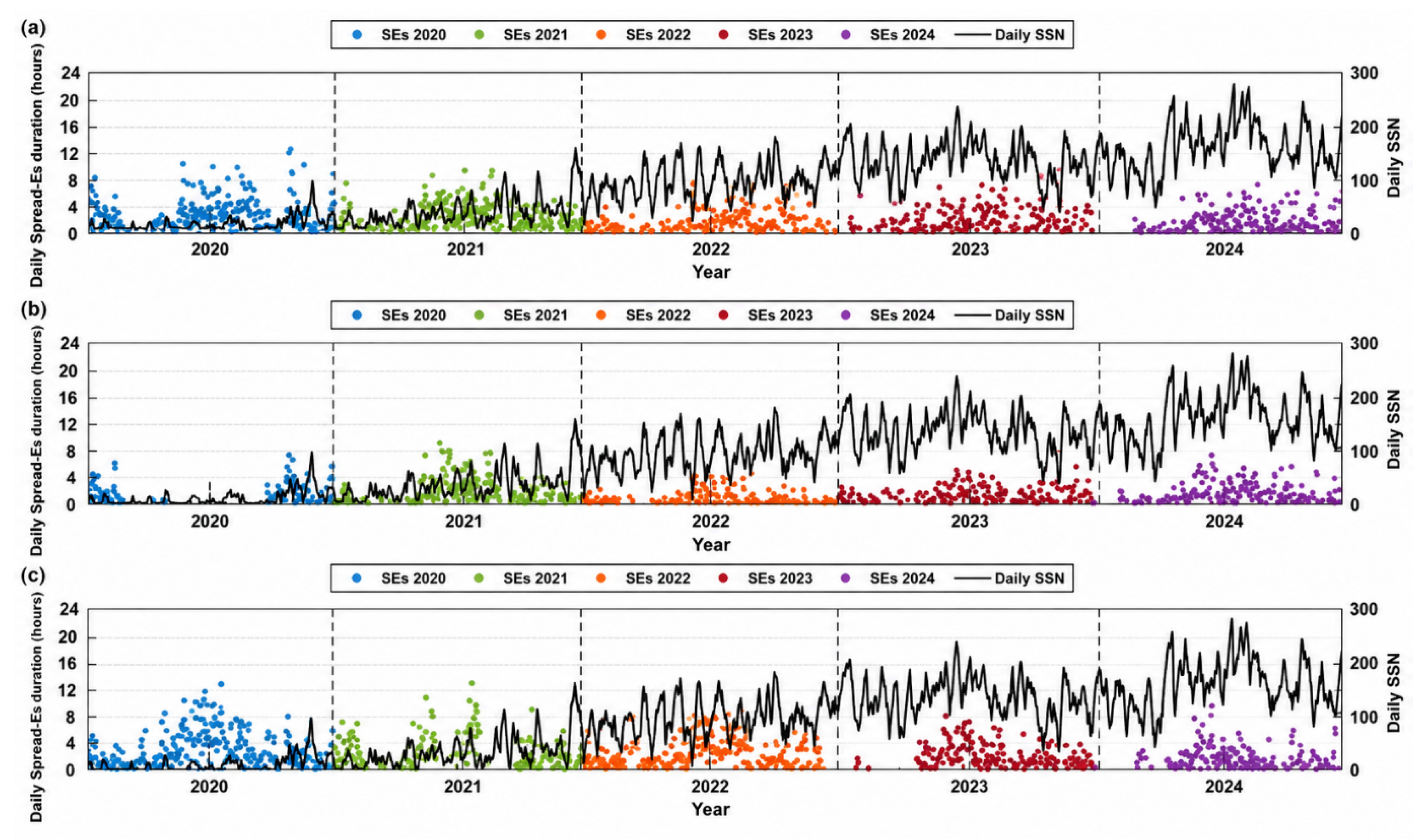
Figure 7 presents the daily Spread-Es duration together with the corresponding daily SSN at Juliusruh, Dourbes, and Roquetes during 2020–2024. The SSN series shows the increase in solar activity from the relatively low levels of 2020–2021 toward higher and more variable values during 2023–2024. Spread-Es duration exhibits pronounced day-to-day, seasonal, and interannual variability at all three stations. However, these variations are superimposed on strong seasonal and local-time dependencies in Spread-Es occurrence and on differences in observational coverage among stations and years.

Figure 7. Daily Spread-Es duration (coloured points) and corresponding daily sunspot number (SSN; black curve) at (a) Juliusruh, (b) Dourbes, and (c) Roquetes during 2020–2024. Different colours represent the individual years, and vertical dashed lines indicate the boundaries between consecutive years. The left vertical axis represents daily Spread-Es duration in hours, while the right vertical axis represents daily SSN. The two quantities are displayed together only to provide solar-activity context; no statistical relationship between SSN and Spread-Es duration is inferred from this figure.

Accordingly, Figure 7 is presented only to place the Spread-Es observations within the solar-activity conditions prevailing during the study period. No correlation or statistical inference regarding solar-activity dependence is derived from this comparison. Establishing such a relationship would require seasonally and local-time controlled occurrence measures, explicit treatment of observational coverage, and a longer observational interval.

3.5. Representative Multi-Station Spread-Es/Spread-F Interval During Regional dTEC Disturbance

A representative interval on 12–13 June 2022 was selected for detailed examination using Digisonde, Height–Time–Intensity (HTI), and dTEC observations.

The 12–13 June 2022 event was selected using the following criteria, applied to the full 2020–2024 dataset:

(i)

Spread-Es was observed simultaneously at all three stations and persisted for an extended period (at least 2 h);

(ii)

Spread-Es and spread-F coexisted at all three stations.

The dTEC structures were not part of the selection criteria; they were examined only after the event had been selected.

Spread-Es was identified at Juliusruh from 19:18 to 22:13 UT, at Dourbes from 21:25 UT on 12 June to 00:40 UT on 13 June, and at Roquetes from 20:25 to 23:55 UT. The Spread-Es duration was approximately 2 h 55 min at Juliusruh, 3 h 15 min at Dourbes, and 3 h 30 min at Roquetes. Spread-Es was simultaneously present at all three stations between 21:25 and 22:13 UT, giving a common multi-station interval of approximately 48 min.

The Kp index ranged from 1.7 to 3.7, representing the level of geomagnetic activity during the days of interest. On 12 June, the Kp index was 2.3 at 19:30 UT and 1.7 at 22:30 UT, increasing to 3.7 at 01:30 UT on 13 June.

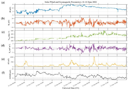
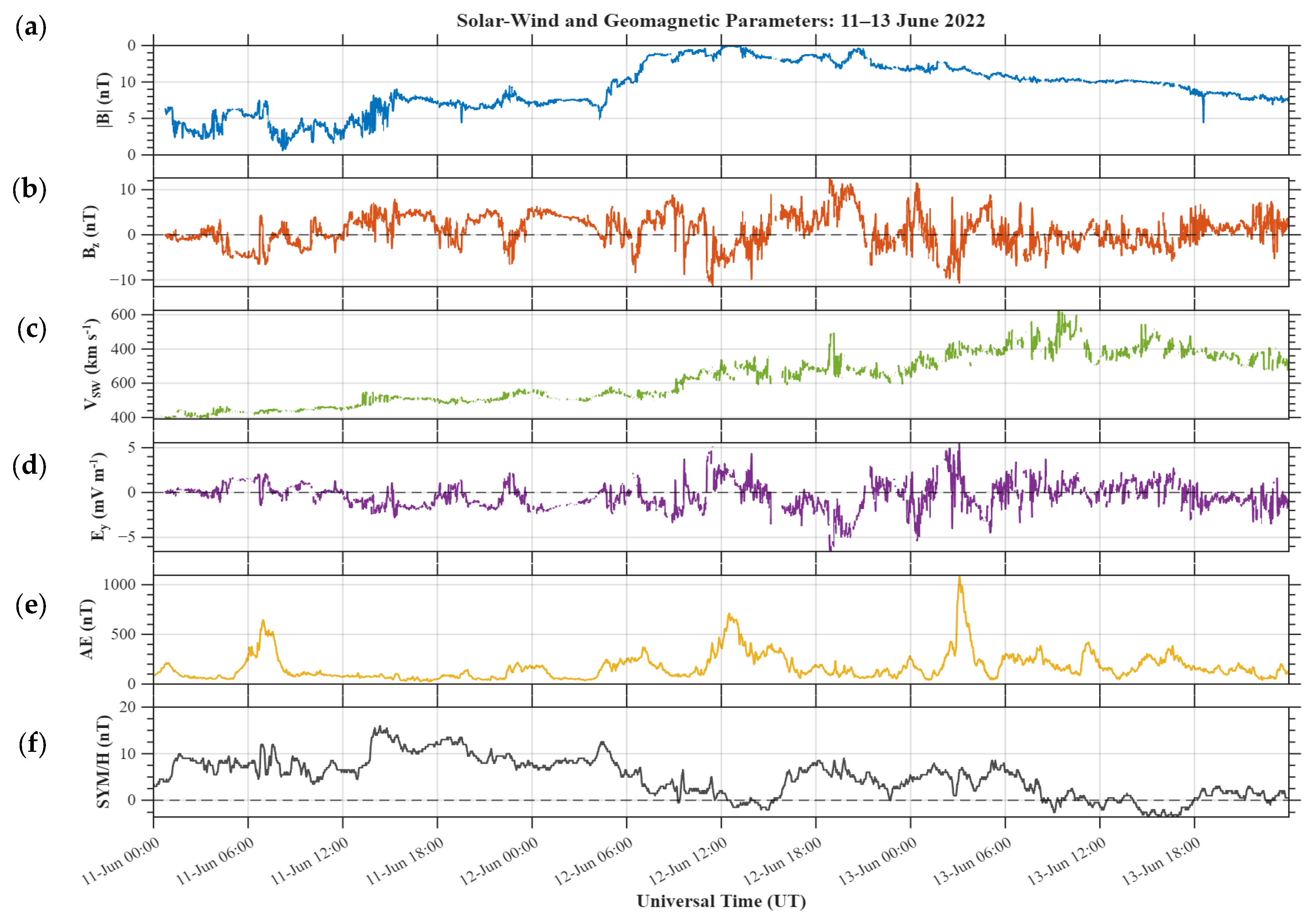
The interplanetary and geomagnetic conditions during 11–13 June 2022 are shown in Figure 8. On 11 June, conditions were quiet, with |B| mostly below 8 nT, a slow solar wind speed of about 300–380 km s⁻¹, and low AE values apart from a short substorm reaching ~650 nT near 07:00 UT. From about 04:00 UT on 12 June, |B| increased steadily, reaching ~15 nT around 12:00 UT, while the solar wind speed rose gradually to ~450 km s⁻¹. This was accompanied by southward excursions of Bz, with a minimum of about −11 nT near 11:30 UT, positive Ey values up to ~5 mV m⁻¹, and an associated increase in AE to ~700 nT around 12:00 UT on 12 June. A second period of southward Bz (down to about −11 nT) occurred between approximately 01:00 and 03:30 UT on 13 June, producing the strongest substorm of the interval, with AE reaching ~1100 nT near 03:15 UT. The solar wind speed continued to increase on 13 June, peaking at ~600 km s⁻¹ around 09:00–10:00 UT, while |B| gradually decreased to ~8 nT by the end of the day.

Figure 8. Interplanetary and geomagnetic conditions during 11–13 June 2022, based on 1min high-resolution OMNI data: (a) IMF magnitude |B|; (b) IMF Bz component (GSM); (c) solar wind speed V_SW; (d) interplanetary electric field Ey; (e) AE index; and (f) SYM-H index. Dashed lines mark zero values.

The Spread-Es observed at the three stations is unlikely to have been driven primarily by geomagnetic forcing. However, the substorm activity, particularly the intense AE enhancement on 13 June, may have contributed to the observed spread-Es through the generation of TIDs propagating equatorward from the auroral zone or through penetration electric fields.

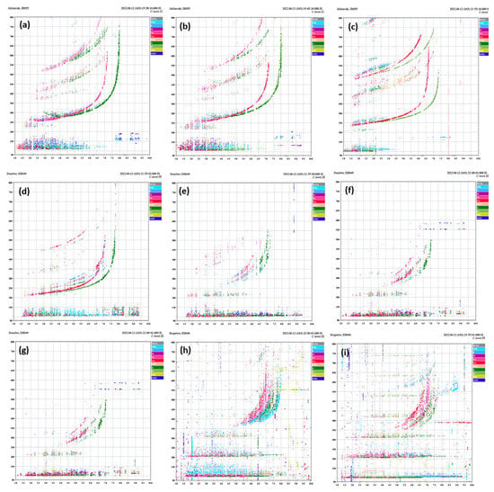
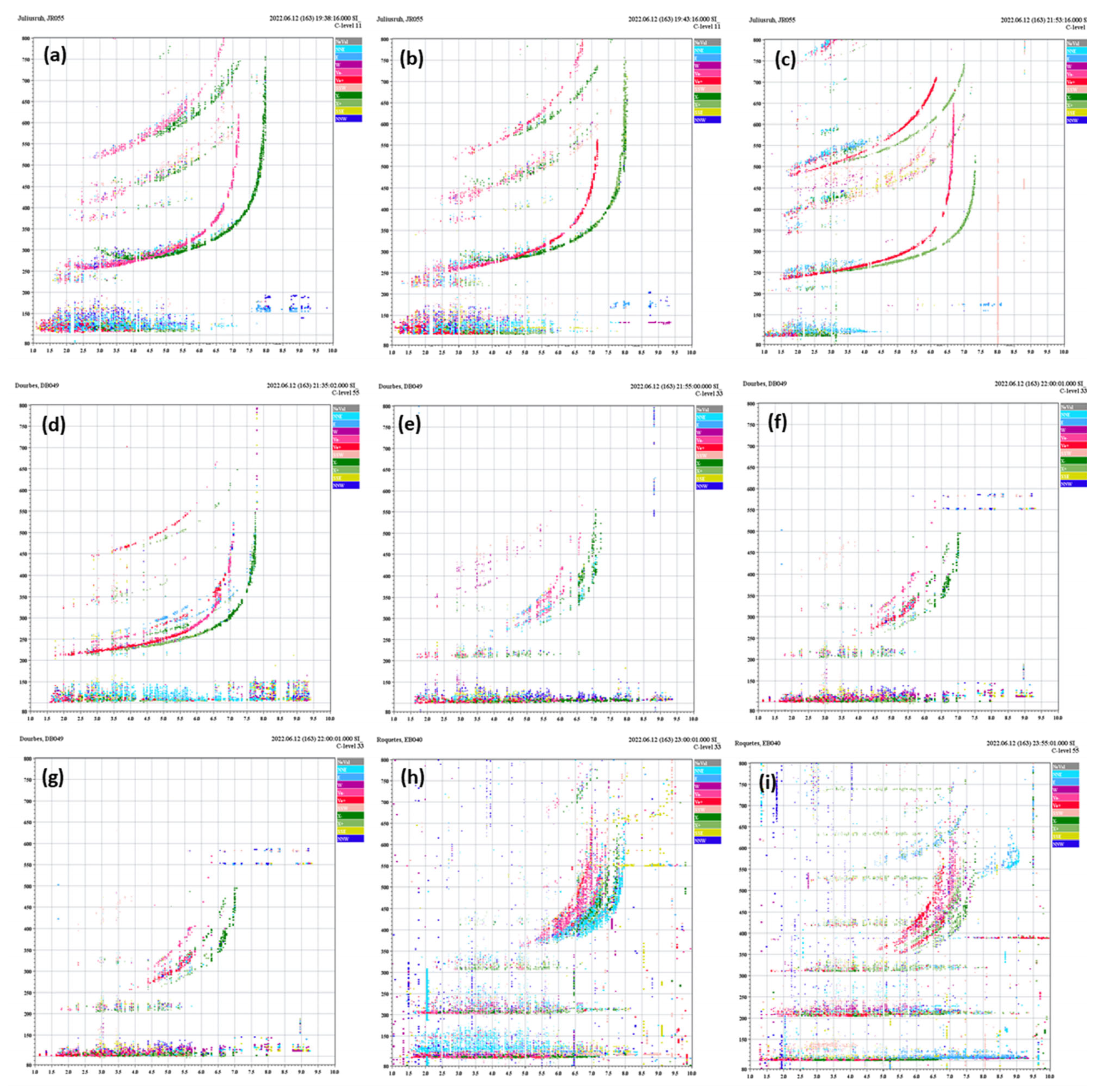
Figure 9 presents representative ionograms obtained during the corresponding Spread-Es intervals. At Juliusruh (Figure 9a–c), pronounced spreading of the Es echoes in virtual range is accompanied by spread-F signatures in the F-region traces. Similar Spread-Es and spread-F signatures are visible in the representative Dourbes ionograms (Figure 9d–f), although the morphology and intensity of the echoes vary throughout the selected interval. At Roquetes (Figure 9g–i), Spread-Es remain evident within the E-region virtual-height range together with pronounced spreading of the F-region echoes. The representative ionograms therefore show coexisting Spread-Es and spread-F signatures at all three stations during the selected event intervals.

Figure 9. Representative ionograms observed during the selected Spread-Es/spread-F interval on 12–13 June 2022. Panels (a–c) correspond to Juliusruh, (d–f) to Dourbes, and (g–i) to Roquetes. The panels illustrate the temporal evolution of Spread-Es and contemporaneous spread-F signatures at the three stations.

The nine panels in Figure 9 correspond to different epochs within the respective station intervals and are not simultaneous measurements across the three stations. The common occurrence interval of 21:25–22:13 UT is determined from the complete manually classified Spread-Es intervals listed in Table 4.

Table 4. Timing of the selected Spread-Es intervals and corresponding dTEC disturbance parameters during 12–13 June 2022.

Station	Spread-Es Start (UT)	Spread-Es End (UT)	Duration	Phase Speed (m s−1)	Period (min)	Horizontal Wavelength (km)
Juliusruh	12 June, 19:18	12 June, 22:13	2 h 55 min	~210	~64	~806
Dourbes	12 June, 21:25	13 June, 00:40	3 h 15 min	~190	~56	~638
Roquetes	12 June, 20:25	12 June, 23:55	3 h 30 min	~180	~48	~518

Note: The dTEC-derived propagation parameters are characteristic event estimates. Their uncertainties are event-dependent and reflect GRID2 spatial sampling and source-product smoothing, finite event duration, temporal sampling, and disturbance-localisation uncertainty; see Section 2.5 and Paul et al. (2026) [22].

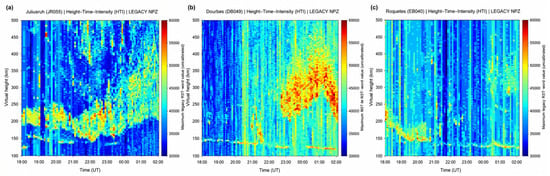
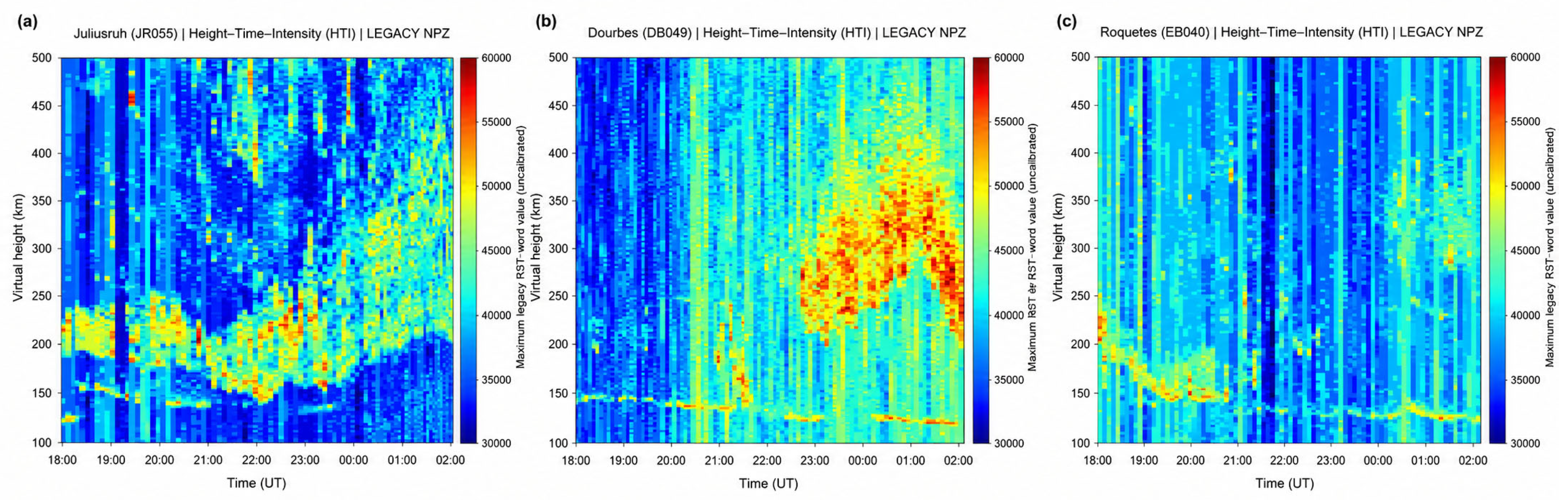
The corresponding HTI representations are shown in Figure 10. At all three stations, the ionospheric echoes exhibit substantial temporal variability over approximately 100–500 km virtual height. At Juliusruh (Figure 10a), the lower virtual-height echo shows a clear sequence of downward and subsequent upward displacement during the evening interval, together with considerable variability at higher virtual heights. At Dourbes (Figure 10b), the lower virtual-height echo varies gradually with time, while enhanced and spatially extended echo intensity develops within the higher virtual-height range during the later part of the interval. At Roquetes (Figure 10c), the lower virtual-height echo also changes with time, while higher virtual-height echoes become more evident during the later portion of the sequence.

Figure 10. Height–Time–Intensity (HTI) representations during the selected 12–13 June 2022 interval at (a) Juliusruh, (b) Dourbes, and (c) Roquetes. Echo intensity is shown as a function of Universal Time and virtual height over approximately 100–500 km, illustrating the temporal evolution of the ionospheric echoes during the selected Spread-Es/spread-F intervals.

The HTI plots show that the selected Spread-Es intervals were accompanied by temporally varying echoes over both the lower and higher virtual-height ranges. The variation is most clearly visible at Juliusruh, while Dourbes and Roquetes show different patterns of temporal and virtual-height variability.

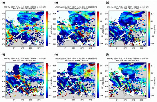
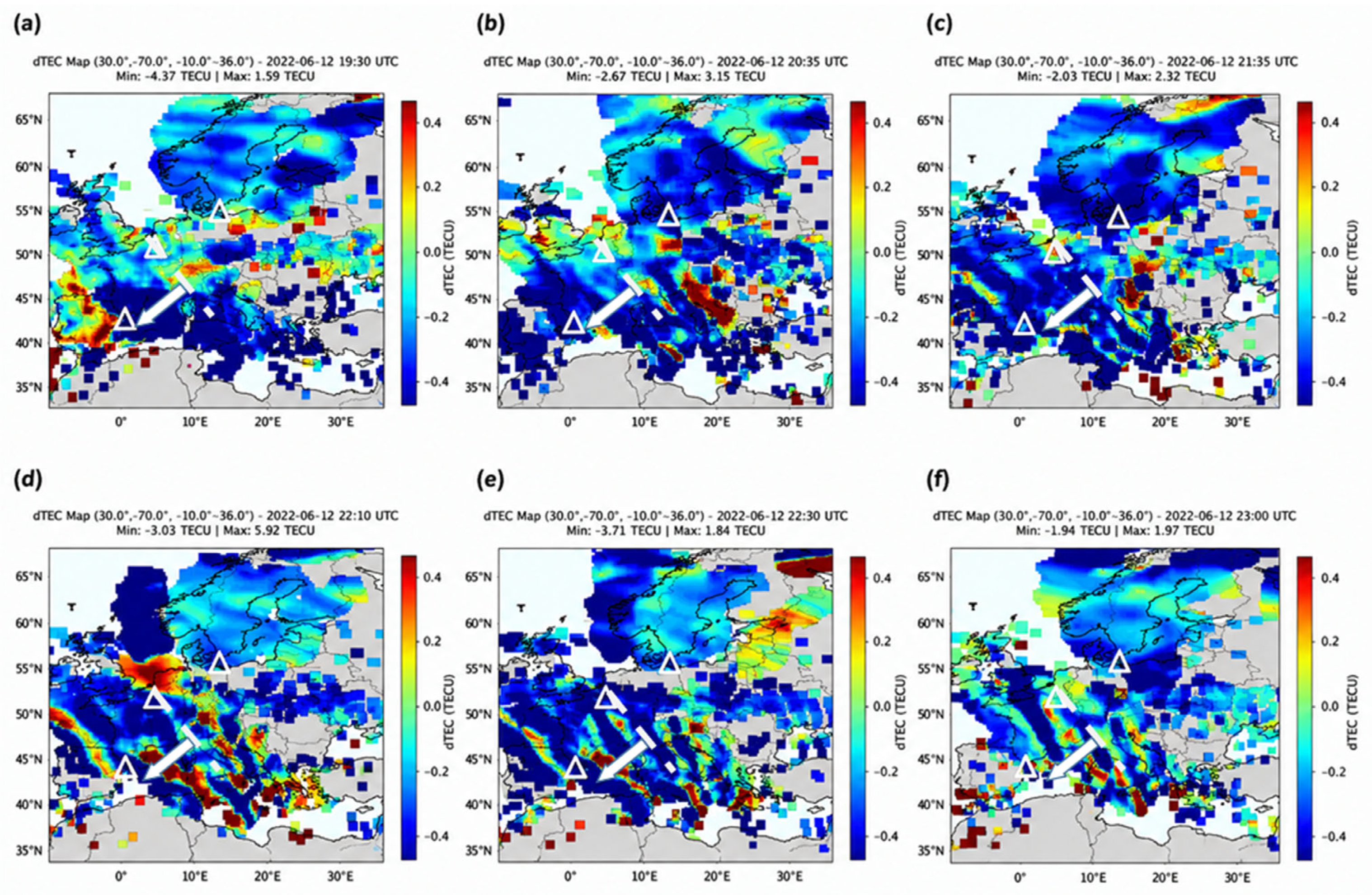
Figure 11 presents the corresponding dTEC observations over the European mid-latitude sector between 19:30 and 23:00 UT on 12 June 2022. Alternating positive and negative dTEC perturbations are visible throughout the sequence, while elongated and organised structures become increasingly evident over central and southern Europe. The phase fronts are predominantly aligned in the northwest–southeast direction, and their displacement between successive maps indicates predominantly southwestward propagation.

Figure 11. Sequence of dTEC maps over the European mid-latitude sector on 12 June 2022 at (a) 19:30, (b) 20:35, (c) 21:35, (d) 22:10, (e) 22:30, and (f) 23:00 UT. The colour scale represents positive and negative dTEC perturbations, while the white triangles mark the locations of Juliusruh, Dourbes, and Roquetes. The panels show the temporal evolution of the regional dTEC structures during the selected interval. Dashed lines indicate successive positions of the tracked same-phase dTEC wavefront, and arrows indicate the corresponding horizontal propagation direction approximately normal to the phase-front orientation.

The temporal evolution of the dTEC structures overlaps the Spread-Es observations at the three stations. At 19:30 UT, Spread-Es was already present at Juliusruh. By 20:35 UT, Spread-Es was present at both Juliusruh and Roquetes. The 21:35 and 22:10 UT dTEC maps fall within the 21:25–22:13 UT interval when Spread-Es was simultaneously present at Juliusruh, Dourbes, and Roquetes. The 22:30 and 23:00 UT maps correspond to the continuing Spread-Es intervals at Dourbes and Roquetes.

Quantitative analysis of the coherent dTEC disturbances yielded characteristic horizontal propagation speeds of approximately 210 m s⁻¹ in the Juliusruh region, 190 m s⁻¹ near Dourbes, and 180 m s⁻¹ near Roquetes. The corresponding dominant periods were approximately 64, 56, and 48 min, respectively. These values give characteristic horizontal wavelengths of approximately 806, 638, and 518 km. The derived parameters should be interpreted within the spatial and temporal resolution of the GRID2 observations and the event-dependent uncertainties described in Section 2.5. The disturbance characteristics obtained for the three station regions are summarised together with the corresponding Spread-Es intervals in Table 4.

4. Discussion

The five-year observations show a clear seasonal and diurnal variation of Spread-Es at Juliusruh, Dourbes, and Roquetes. At all three stations, Spread-Es occurrence is higher during summer than during winter and is observed mainly during nighttime. The summer occurrence is 16.9% at Juliusruh, 12.5% at Roquetes, and 8.6% at Dourbes, while the corresponding winter values are 5.6%, 4.8%, and 2.6%, respectively. The monthly–hourly distributions also show the highest peak occurrence at Juliusruh, while Roquetes exhibits a broader nighttime distribution. These results indicate a common summer and nighttime preference, together with clear differences among the three stations.

The pronounced summer enhancement is consistent with the well-established seasonal behaviour of mid-latitude sporadic-E. In the classical wind-shear mechanism, long-lived metallic ions of meteoric origin are converged by neutral-wind shears to form Es layers [1,2,3,4]. Haldoupis et al. (2007) [5] further showed that the strong summer maximum of mid-latitude Es is related to the seasonal variation of meteoric metallic-ion input. However, the present study concerns Spread-Es rather than ordinary Es occurrence. The processes responsible for the formation of an Es layer should therefore be distinguished from those producing the spatial structuring responsible for its spread appearance in ionograms.

Atmospheric-wave modulation is one process capable of producing such additional structure. The representative Dourbes ionograms in Figure 4 show that the broadened Es echoes are accompanied by off-vertical echoes identified from their different direction-of-arrival colour coding. These off-vertical echoes are present throughout the sequence in Figure 4a–c, with westward (W) and north-northwestward (NNW) echoes particularly evident within the Spread-Es region and additional directionally separated echoes appearing at different frequencies and times. Their occurrence together with the increasing virtual-range spreading shows that the Spread-Es morphology involves echoes arriving from several directions rather than only the principal near-vertical Es echo. Such behaviour is consistent with a spatially structured, tilted, or horizontally inhomogeneous Es layer capable of producing multiple propagation paths. Barnes (1992) [23] showed that structured Spread-Es can produce multiple refracted propagation paths, while Chen et al. (2011) [9] showed that gravity waves can deform and tilt an existing Es layer, producing moving plasma structures and off-vertical HF echoes that appear as Spread-Es. Chen et al. (2011) [9] also found a common periodicity of approximately 35 min in Es-related parameters, linking the spread morphology to wave-modulated Es structures. These observations provide a possible mechanism through which an existing Es layer can become tilted or horizontally structured. However, although the off-vertical echoes observed in Figure 3 demonstrate the directional complexity of the Spread-Es morphology, they do not by themselves identify the physical process responsible for the Es structuring, and the five-year climatology presented here does not establish that the observed Spread-Es occurrences were produced by gravity waves or TIDs.

The nighttime preference should likewise not be attributed to a single mechanism. Otsuka et al. (2007) [6] observed nighttime MSTIDs together with E-region field-aligned irregularities, while Otsuka et al. (2008) [7] reported a statistical relationship between nighttime MSTIDs and sporadic-E activity during summer. These studies demonstrate that nighttime MSTID activity and structured E-region plasma can occur together, although the climatological observations in the present study do not determine the mechanism responsible for individual Spread-Es intervals.

The differences among the three stations also require cautious interpretation. Juliusruh shows the highest summer occurrence and the highest peak monthly–hourly occurrence, while Roquetes exhibits a broader nighttime distribution and Dourbes generally shows lower values. This variation does not follow a simple monotonic pattern with latitude. In addition, observational coverage differs among stations and years, particularly at Dourbes. The present results therefore show regional differences in Spread-Es occurrence, but these differences cannot be attributed uniquely to latitude. Neutral winds, tides, atmospheric-wave activity, geomagnetic conditions, and the local electrodynamic environment may all contribute, but these parameters were not examined directly in the present climatological analysis.

The SSN observations are included only to place the 2020–2024 Spread-Es climatology within the ascending phase of Solar Cycle 25. No statistical relationship between Spread-Es and solar activity is inferred from the present dataset because the strong seasonal and local-time dependence of Spread-Es, together with non-uniform observational coverage and the limited solar-cycle interval, would confound a direct comparison. A dedicated assessment of solar dependence would require these effects to be controlled explicitly and would benefit from observations spanning a longer portion of the solar cycle.

The 12–13 June 2022 interval provides additional information on the ionospheric conditions accompanying Spread-Es. During this interval, Spread-Es and spread-F signatures were observed at all three stations, with Spread-Es simultaneously present at Juliusruh, Dourbes, and Roquetes between 21:25 and 22:13 UT. The HTI plots show temporal changes in the echoes over the lower and higher virtual-height ranges. These variations describe the temporal evolution of the ionospheric echoes but do not by themselves identify a TID.

The independent dTEC observations show organised electron-density perturbations with predominantly NW–SE-oriented phase fronts and southwestward propagation. Quantitative characterisation gives horizontal propagation speeds of approximately 180–210 m s⁻¹, dominant periods of approximately 48–64 min, and estimated horizontal wavelengths of approximately 518–806 km. These values are consistent with nighttime MSTID-scale disturbances and should be interpreted within the event-dependent spatial and temporal resolution of the GRID2 analysis described in Section 2.5.

The scale classification is based on the combined temporal and spatial characteristics rather than on a single parameter. Paul et al. (2026) [22] reported nighttime MSTID-associated horizontal wavelengths of approximately 295–782 km in 2020 and 230–850 km in 2024 at Dourbes, as well as approximately 196–600 km in 2020 and 216–540 km in 2024 at Roquetes. The present wavelengths of approximately 806, 638, and 518 km therefore lie within or near the upper part of the European nighttime MSTID ranges reported in that study. The corresponding propagation speeds of approximately 180–210 m s⁻¹ fall within the characteristic MSTID range of about 50–400 m s⁻¹. The periods of approximately 56 and 48 min at Dourbes and Roquetes are also within the commonly used 15–60 min interval, whereas the approximately 64 min period near Juliusruh lies close to and slightly above this nominal temporal boundary. Accordingly, the disturbance is described here as a nighttime MSTID-scale event based on the combined period, propagation speed, wavelength, propagation direction, and phase-front orientation, rather than on any single parameter. The selected Spread-Es/spread-F interval therefore occurred in the presence of nighttime MSTID activity over the European sector.

The simultaneous presence of nighttime MSTID activity, Spread-Es, and spread-F is particularly relevant to the electrodynamic framework proposed for the nighttime mid-latitude ionosphere. Tsunoda and Cosgrove (2001) [24] described a coupled response initiated in the presence of a TID, in which F-region plasma structuring produces corresponding structure in the E region. Hall-current polarisation associated with the structured Es layer can then generate polarisation electric fields that map along the geomagnetic field lines to the F region and reinforce the F-region disturbance. In this framework, the E- and F-region responses are therefore not independent, but can form part of a coupled electrodynamic system.

Cosgrove and Tsunoda (2004) [11] subsequently showed theoretically that the Es-layer and F-region Perkins instabilities can interact as a coupled system through electric fields mapping between the two regions. Their analysis showed that the coupled system has a greater growth rate than the individual instabilities considered separately, particularly enhancing F-region structuring. Tsunoda (2006) [12] further showed that polarisation electric fields generated by the Es-layer instability can map to the F region and enhance its vertical plasma motion and instability growth, while the F-region Pedersen conductivity also influences the E-region response. Thus, under suitable nighttime conditions, structured Es and F-region disturbances can interact through a two-way electrodynamic response rather than evolving independently.

Observational evidence for such interaction was presented by Haldoupis et al. (2003) [10], who reported a close relationship between unstable, spatially structured sporadic-E and mesoscale spread-F. They proposed that enhanced polarisation electric fields generated within unstable Es patches can map upward along the geomagnetic field and produce E × B plasma motion and structuring in the F region. Their companion case studies also observed patchy sporadic-E, spread-F, and TIDs simultaneously and interpreted these observations in terms of upward mapping of E-region polarisation electric fields [25].

The observations on 12–13 June 2022 contain the same principal ionospheric components considered in these earlier studies: nighttime MSTID activity detected independently in dTEC together with Spread-Es and spread-F signatures in the ionograms. The event is therefore compatible with the conditions under which E–F electrodynamic coupling has previously been proposed and observed. However, the present observations cannot establish that this coupling mechanism operated during the event. Measurements of the polarisation electric field, Hall and Pedersen conductivities, currents, or the two-dimensional motion and orientation of the Es structures are not available. The present case therefore shows the coexistence of the required ionospheric signatures, while the actual electrodynamic connection between the E and F regions remains unresolved.

A propagation-related interpretation must also be retained. Barnes (1992) [23] showed that spatially structured Spread-Es can refract HF signals along multiple propagation paths toward the F region, producing apparent fine structure in F-region echoes. Consequently, some of the spread-F morphology observed together with Spread-Es in Figure 7 may be influenced by propagation through the structured Es layer. The regional dTEC observations independently confirm that the F-region electron-density field was disturbed during the event, but they cannot determine the origin of each spread-F trace observed in the ionograms.

The 12–13 June 2022 interval is presented as an illustrative case study, selected because Spread-Es persisted for an extended period and coexisted with spread-F at all three stations, during independently detected nighttime MSTID activity. It is therefore not intended to establish a statistical or causal relationship between Spread-Es and MSTIDs. Previous observational and theoretical studies have reported associations among structured sporadic-E layers, mid-latitude spread-F and travelling ionospheric disturbances [10,23], including a statistical relationship between nighttime MSTID activity and sporadic-E activity and Otsuka et al. (2008) [7], and have shown that such conditions can support electrodynamic interaction between the E and F regions through polarisation electric-field mapping [10,11,12,25,26,27,28]. At the same time, propagation through structured Spread-Es may contribute to the observed F-region ionogram morphology [21]. A single event cannot determine whether the observed Spread-Es was generated by the MSTID, whether the simultaneous E- and F-region structures resulted from direct electrodynamic coupling, or how much propagation effects contributed. The dTEC analysis is therefore used only to identify and characterise the regional MSTID present during the event.

The principal limitations of the present analysis arise from the available observations. The five-year climatology is based on Digisonde morphology and therefore describes Spread-Es occurrence rather than the two-dimensional structure or physical thickness of the Es layer. The HTI representations describe echo intensity as a function of virtual height and time and are not independent measurements of TID activity. The dTEC analysis is restricted to the selected 12–13 June 2022 interval and therefore does not establish a climatological relationship between Spread-Es and MSTIDs. The non-uniform observational coverage also affects some station and interannual comparisons, while the SSN comparison remains descriptive rather than statistical.

5. Conclusions

This study presents a five-year climatological investigation of Spread-Es over the European mid-latitude ionosphere using Digisonde observations from Juliusruh, Dourbes, and Roquetes during 2020–2024. The principal findings are:

• Seasonal and diurnal behaviour. Spread-Es shows a pronounced summer enhancement and nighttime preference at all three stations. Summer occurrence reaches 16.9% at Juliusruh, 12.5% at Roquetes, and 8.6% at Dourbes, compared with winter values of 5.6%, 4.8%, and 2.6%, respectively.
• Station-to-station variability. The maximum monthly–hourly occurrence rate is highest at Juliusruh (≈0.48), followed by Roquetes (≈0.40) and Dourbes (≈0.35). Roquetes exhibits a broader nighttime interval of enhanced Spread-Es occurrence extending farther into the post-midnight hours.
• Solar-activity context. Daily SSN is included to characterise the solar-activity conditions during the ascending phase of Solar Cycle 25. Because seasonal, local-time, interannual, and observational-coverage effects are not statistically separated from SSN, no quantitative inference regarding solar-activity dependence is made from the present dataset.
• Representative multi-station event. During 12–13 June 2022, Spread-Es persisted for approximately 3 h at each station and was simultaneously present at Juliusruh, Dourbes, and Roquetes from 21:25 to 22:13 UT, together with spread-F. Independent dTEC observations showed predominantly southwestward propagation with NW–SE-oriented phase fronts, characteristic horizontal speeds of approximately 180–210 m s⁻¹, periods of approximately 48–64 min, and estimated wavelengths of approximately 518–806 km. Taken together, these characteristics support interpretation of the disturbance as a nighttime MSTID-scale event over the European sector.
• Physical interpretation and limitations. The simultaneous occurrence of Spread-Es, spread-F, and independently observed nighttime MSTID-scale activity is compatible with previously proposed E–F electrodynamic coupling mechanisms, but the present observations do not establish that such coupling occurred. Measurements of electric fields, currents, conductivities, and the two-dimensional structure and motion of the Es layer were not available, and propagation through structured Spread-Es may also influence the observed F-region ionogram morphology. Further multi-instrument observations are required to determine the physical relationship among these phenomena.

References

- Whitehead, J.D. The formation of the sporadic-E layer in the temperate zones. J. Atmos. Terr. Phys. 1961, 20, 49–58. [Google Scholar] [CrossRef] [Scilit]
- Haldoupis, C. Midlatitude sporadic E. A typical paradigm of atmosphere–ionosphere coupling. Space Sci. Rev. 2012, 168, 441–461. [Google Scholar] [CrossRef] [Scilit]
- Axford, W.I. The formation and vertical movement of dense ionized layers in the ionosphere due to neutral wind shears. J. Geophys. Res. 1963, 68, 769–779. [Google Scholar] [CrossRef] [Scilit]
- Mathews, J.D. Sporadic E: Current views and recent progress. J. Atmos. Sol.-Terr. Phys. 1998, 60, 413–435. [Google Scholar] [CrossRef] [Scilit]
- Haldoupis, C.; Pancheva, D.; Singer, W.; Meek, C.; MacDougall, J. An explanation for the seasonal dependence of midlatitude sporadic E layers. J. Geophys. Res. Space Phys. 2007, 112, A06315. [Google Scholar] [CrossRef] [Scilit]
- Otsuka, Y.; Onoma, F.; Shiokawa, K.; Ogawa, T.; Yamamoto, M.; Fukao, S. Simultaneous observations of nighttime medium-scale traveling ionospheric disturbances and E region field-aligned irregularities at midlatitude. J. Geophys. Res. Space Phys. 2007, 112, A06317. [Google Scholar] [CrossRef] [Scilit]
- Otsuka, Y.; Tani, T.; Tsugawa, T.; Ogawa, T.; Saito, A. Statistical study of relationship between medium-scale traveling ionospheric disturbance and sporadic E layer activities in summer night over Japan. J. Atmos. Sol.-Terr. Phys. 2008, 70, 2196–2202. [Google Scholar] [CrossRef] [Scilit]
- Wei, L.; Jiang, C.; Hu, Y.; Aa, E.; Huang, W.; Liu, J.; Yang, G.; Zhao, Z. Ionosonde observations of spread F and spread Es at low and middle latitudes during the recovery phase of the 7–9 September 2017 geomagnetic storm. Remote Sens. 2021, 13, 1010. [Google Scholar] [CrossRef] [Scilit]
- Chen, G.; Zhao, Z.; Zhang, Y.; Yang, G.; Zhou, C.; Huang, S.; Li, T.; Li, N.; Sun, H. Gravity waves and spread Es observed during the solar eclipse of 22 July 2009. J. Geophys. Res. Space Phys. 2011, 116, A09314. [Google Scholar] [CrossRef] [Scilit]
- Haldoupis, C.; Kelley, M.C.; Hussey, G.C.; Shalimov, S. Role of unstable sporadic-E layers in the generation of midlatitude spread F. J. Geophys. Res. Space Phys. 2003, 108, 1446. [Google Scholar] [CrossRef] [Scilit]
- Cosgrove, R.B.; Tsunoda, R.T. Instability of the E–F coupled nighttime midlatitude ionosphere. J. Geophys. Res. Space Phys. 2004, 109, A04305. [Google Scholar] [CrossRef] [Scilit]
- Tsunoda, R.T. On the coupling of layer instabilities in the nighttime midlatitude ionosphere. J. Geophys. Res. Space Phys. 2006, 111, A11304. [Google Scholar] [CrossRef] [Scilit]
- Reinisch, B.W.; Galkin, I.A. Global Ionospheric Radio Observatory (GIRO). Earth Planets Space 2011, 63, 377–381. [Google Scholar] [CrossRef] [Scilit]
- Khmyrov, G.M.; Galkin, I.A.; Kozlov, A.V.; Reinisch, B.W.; McElroy, J.; Dozois, C. Exploring Digisonde ionogram data with SAO-X and DIDBase. AIP Conf. Proc. 2008, 974, 175–185. [Google Scholar] [CrossRef] [Scilit]
- Piggott, W.R.; Rawer, K. URSI Handbook of Ionogram Interpretation and Reduction; URSI commission III: Warsaw, Poland, 1972. [Google Scholar]
- Wakai, N.; Ohyama, H.; Koizumi, T. Manual of Ionogram Scaling; Radio Research Laboratory, Ministry of Posts and Telecommunications: Tokyo, Japan, 1987. [Google Scholar]
- Zhou, C.; Tang, Q.; Huang, F.; Liu, Y.; Gu, X.; Lei, J.; Ni, B.; Zhao, Z. The simultaneous observations of nighttime ionospheric E region irregularities and F region medium-scale traveling ionospheric disturbances in midlatitude China. J. Geophys. Res. Space Phys. J. Geophys. Res. Space Phys. 2018, 123, 5195–5209. [Google Scholar] [CrossRef] [Scilit]
- Moro, J.; Xu, J.; Bageston, J.V.; Da Silva, L.A.; Resende, L.C.; De Nardin, C.M.; Andrioli, V.F.; Santos, A.M.; Picanço, G.A.; Li, H.; et al. Study of height-spread sporadic-E layers observed in the South American Magnetic Anomaly. Front. Astron. Space Sci. 2025, 12, 1535186. [Google Scholar] [CrossRef] [Scilit]
- Haldoupis, C.; Meek, C.; Christakis, N.; Pancheva, D.; Bourdillon, A. Ionogram height–time–intensity observations of descending sporadic E layers at mid-latitude. J. Atmos. Sol.-Terr. Phys. 2006, 68, 539–557. [Google Scholar] [CrossRef] [Scilit]
- Otsuka, Y.; Ogawa, T.; Saito, A.; Tsugawa, T.; Fukao, S.; Miyazaki, S. A new technique for mapping of total electron content using GPS network in Japan. Earth Planets Space 2002, 54, 63–70. [Google Scholar] [CrossRef] [Scilit]
- Otsuka, Y.; Suzuki, K.; Nakagawa, S.; Nishioka, M.; Shiokawa, K.; Tsugawa, T. GPS observations of medium-scale traveling ionospheric disturbances over Europe. Ann. Geophys. 2013, 31, 163–172. [Google Scholar] [CrossRef] [Scilit]
- Paul, K.S.; Altadill, D.; Nandakumar, A.; Haralambous, H.; Verhulst, T.G.; Mathew, T.J. Evaluation of Oblique and Fork Traces in Ionograms as Indicators of MSTIDs and Their Relationship to the Development of Spread-F at European Mid-Latitudes. Atmosphere 2026, 17, 866. [Google Scholar] [CrossRef] [Scilit]
- Barnes, R.I. Spread-Es structure producing apparent small-scale structure in the F-region. J. Atmos. Terr. Phys. 1992, 54, 373–389. [Google Scholar] [CrossRef] [Scilit]
- Tsunoda, R.T.; Cosgrove, R.B. Coupled electrodynamics in the nighttime midlatitude ionosphere. Geophys. Res. Lett. 2001, 28, 4171–4174. [Google Scholar] [CrossRef] [Scilit]
- Kelley, M.C.; Haldoupis, C.; Nicolls, M.J.; Makela, J.J.; Belehaki, A.; Shalimov, S.; Wong, V.K. Case studies of coupling between the E and F regions during unstable sporadic-E conditions. J. Geophys. Res. Space Phys. 2003, 108, 1447. [Google Scholar] [CrossRef] [Scilit]
- Bowman, G.G. Some aspects of mid-latitude spread-Es, and its relationship with spread-F. Planet. Space Sci. 1985, 33, 1081–1089. [Google Scholar] [CrossRef] [Scilit]
- Perkins, F. Spread F and ionospheric currents. J. Geophys. Res. 1973, 78, 218–226. [Google Scholar] [CrossRef] [Scilit]
- Zhou, Q.; Mathews, J.D. On the physical explanation of the Perkins instability. J. Geophys. Res. Space Phys. 2006, 111, A12309. [Google Scholar] [CrossRef] [Scilit]
Disclaimer/Publisher’s Note: The statements, opinions and data contained in all publications are solely those of the individual author(s) and contributor(s) and not of MDPI and/or the editor(s). MDPI and/or the editor(s) disclaim responsibility for any injury to people or property resulting from any ideas, methods, instructions or products referred to in the content. |
© 2026 by the authors. Licensee MDPI, Basel, Switzerland. This article is an open access article distributed under the terms and conditions of the Creative Commons Attribution (CC BY) license.