Development and Evaluation of a 1.5 km CorrDiff Downscaling System for the Korean Peninsula

Abstract

To downscale artificial intelligence (AI) medium-range forecasts over the Korean Peninsula, we developed a 1.5 km CorrDiff system trained with ERA5 inputs and UM-LDAPS analyses as targets. For 1.5 m temperature and 10 m wind, the regression stage reduced root-mean-square error (RMSE) and root-mean-square vector error (RMSVE) relative to ERA5 and increased spatial correlation. CorrDiff had smaller absolute biases and greater spatial variability than Regression but higher RMSE and RMSVE and lower spatial correlation. The most consistent improvement relative to Regression occurred for high-temperature events at or above the target 99th percentile, with higher probability of detection (POD) and critical success index (CSI) and lower conditional temperature error. Without additional training or correction, AI Forecasting System (AIFS) forecasts were downscaled through +288 h. In a July 2026 heatwave case at 47 stations, CorrDiff reduced temperature errors and alleviated the underprediction of high-temperature occurrence relative to Regression. CorrDiff had higher POD and CSI than the AIFS for temperatures ≥33 °C but higher RMSE and lower spatial correlation. Generative downscaling should therefore be evaluated for spatial variability, spatial agreement, and event-specific performance beyond deterministic errors; producing high-resolution data does not necessarily imply improved forecast performance against observations.

1. Introduction

Global artificial intelligence (AI) weather prediction models have advanced rapidly, and medium-range forecast performance comparable to or exceeding that of conventional numerical weather prediction (NWP) models has been reported [1,2]. However, the spatial resolution of global forecast fields may be insufficient to represent detailed spatial distributions of temperature and wind at regional scales. Studies have therefore downscaled global meteorological fields to high resolution [3,4], and downscaling can serve as a means of converting medium-range forecast information from global AI models into high-resolution data for regional use.

The Korean Peninsula has complex mountainous terrain, coastlines, and diverse surface characteristics within a relatively small area, where local weather phenomena are strongly influenced by terrain and surface conditions. In mountainous regions, local strong winds can be generated by atmospheric flow modified by the terrain [5], and in urban areas, the characteristics of high temperatures can vary with interactions between urban heat islands and heatwaves [6]. Producing high-resolution forecast data for the Korean Peninsula therefore requires downscaling techniques that can reflect these local meteorological characteristics.

Various methods, including traditional statistical techniques and machine learning, have been used to downscale meteorological fields [7]. In deterministic models trained to minimize the mean squared error, small-scale variability that is difficult to determine from low-resolution inputs alone can appear weaker than in the target [3]. Generative models can represent such variability by learning the conditional probability distribution of high-resolution fields given low-resolution inputs [3,8]. Examples include stochastic downscaling of meteorological fields with a generative adversarial network (GAN) [9] and diffusion-model emulation of high-resolution precipitation fields from climate simulations [10].

CorrDiff, proposed by Mardani et al. [3], is a two-stage generative downscaling model: its regression stage predicts high-resolution fields from low-resolution inputs, and its diffusion stage learns and generates the residual between the regression prediction and the target. Originally presented for the Taiwan region [3], CorrDiff has since been applied to other regions [4,11], and AI-based global precipitation forecasts have also been downscaled to high-resolution precipitation fields [12]. For South Korea, the production of temperature fields at 1 km grid spacing with a machine-learning-based deterministic downscaling method has been reported [13]. However, evaluating CorrDiff for producing high-resolution medium-range forecast data over the Korean Peninsula requires distinguishing between the regression output and the final CorrDiff output. It is also necessary to examine how the spatial variability added by the diffusion stage is associated with changes in deterministic errors and spatial agreement. How these changes vary across variables and event intensities should likewise be examined. Furthermore, it remains necessary to evaluate how these characteristics appear when a downscaling system trained on reanalysis data is applied to forecast fields.

In this study, we developed a 1.5 km CorrDiff generative downscaling system for the Korean Peninsula to produce high-resolution medium-range forecast data for regional use. The model was trained with 0.25° gridded fields from ERA5, the fifth-generation atmospheric reanalysis of the European Centre for Medium-Range Weather Forecasts (ECMWF), as inputs. The targets were 1.5 km operational analyses from the Unified Model–Local Data Assimilation and Prediction System (UM-LDAPS), the local forecasting system of the Korea Meteorological Administration (KMA). Terrain elevation and a land–sea mask were used as static inputs. First, for 1.5 m temperature and 10 m wind, we compared the deterministic errors, value distributions, spatial variability, and spatial agreement of ERA5, the regression output, and the final CorrDiff output to distinguish the effects of the regression and diffusion stages. Second, we evaluated how the effects of the diffusion stage vary with event type and intensity for low-temperature, high-temperature, and strong-wind events. Finally, the ERA5-trained system was applied without additional training or correction to forecast fields from the ECMWF AI Forecasting System (AIFS) to produce 1.5 km medium-range forecast data for the Korean Peninsula through +288 h. For a July 2026 heatwave case, temperature errors, spatial correlation, and high-temperature detection performance were evaluated against Automated Synoptic Observing System (ASOS) temperature observations.

2. Materials and Methods

2.1. Study Area and Data

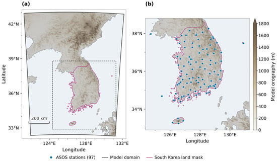
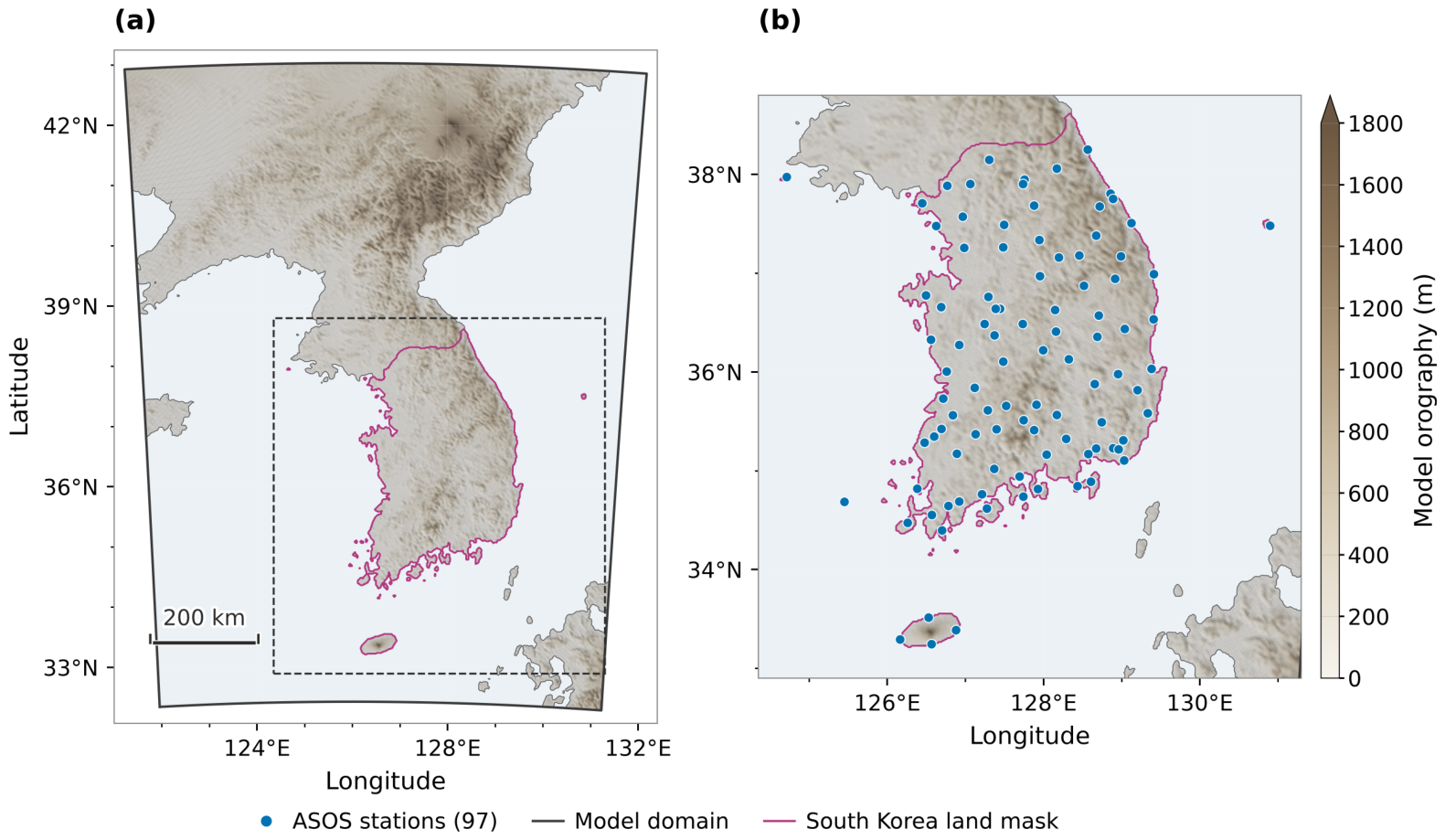
The model domain covers the entire Korean Peninsula, parts of neighboring China and Japan, and the surrounding seas and consists of 768 × 576 grid points with a horizontal grid spacing of 1.5 km. The model terrain, land–sea distribution, and locations of the 97 ASOS stations considered for the AIFS application evaluation are shown in Figure 1.

Figure 1. Model domain, static input fields, and observational network used for verification. (a) Model terrain, coastline, the South Korean land area used for grid-based evaluation, and the boundary of the full 768 × 576 model domain. The dashed rectangle indicates the area enlarged in (b). (b) Locations of the 97 ASOS stations, including Baengnyeongdo and Ulleungdo.

As inputs, we used 13 variables at the surface and at the 925 and 850 hPa pressure levels from the ERA5 reanalysis [14] at 0.25° grid spacing (Table 1). ERA5 was bilinearly interpolated onto the UM-LDAPS grid, which is based on the Lambert conformal conic (LCC) projection; hereafter, ERA5 refers to these regridded input fields. This regridding aligns the coarse-resolution meteorological inputs with the 1.5 km UM-LDAPS target grid, as required by the CorrDiff implementation adopted in this study. The interpolation itself does not introduce new fine-scale meteorological information.

Table 1. ERA5 input variables, static inputs, and output variables used for CorrDiff training.

Category	Level	Variables	Variable Names
ERA5 input	Surface	Mean sea-level pressure, skin temperature, 2 m air temperature, 10 m zonal and meridional winds	msl, skt, t2m, u10, v10
	925 hPa	Temperature, geopotential, zonal and meridional winds	t925, z925, u925, v925
	850 hPa	Temperature, geopotential, zonal and meridional winds	t850, z850, u850, v850
Static input	—	Terrain elevation, land–sea mask	terrain, landmask
Output	Surface	1.5 m air temperature, surface temperature, mean sea-level pressure, 10 m zonal and meridional winds	t1p5m, tsfc, mslp, u10, v10
	925 hPa	Zonal and meridional winds	u925, v925
	850 hPa	Zonal and meridional winds	u850, v850

The 1.5 km UM-LDAPS operational analyses of the KMA [15] were used as the target for high-resolution training and as the reference for the grid-based evaluation; hereafter, these analyses are referred to as the target. The meteorological fields used for model weight training, validation, and the grid-based evaluation cover the period from 7 June 2018 to 28 February 2026.

CorrDiff outputs nine variables at the surface and at the 925 and 850 hPa pressure levels, as detailed in Table 1. The 10 m wind speed was calculated at each grid point from the 10 m zonal and meridional wind components as $WS10=\sqrt{u_{10}^2+v_{10}^2}$. The terrain elevation and land–sea mask of the target grid were used as static inputs. The land–sea mask is the fraction of land in each grid cell (land fraction): 0 for ocean, 1 for land, and intermediate values for coastal grid cells.

2.2. Model Configuration and Training

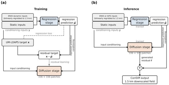
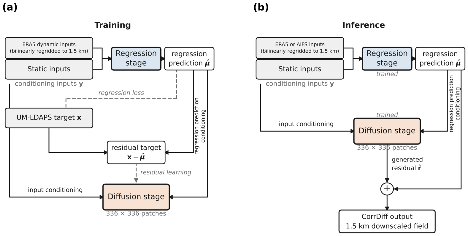
We applied the CorrDiff of Mardani et al. [3] to the Korean Peninsula model domain (Figure 1a); the training and inference workflow is shown in Figure 2. The regression stage is a deterministic U-Net based on SongUNet that predicts high-resolution fields from ERA5 and the static inputs. The numbers of grid points in the x and y directions of the model domain were each set to a multiple of $2^4$ to accommodate the four spatial downsampling steps of the encoder. The domain was configured with 768 × 576 grid points, retaining as much of the UM-LDAPS domain as possible. Self-attention was applied at the lowest encoder resolution of 48 × 36 grid points. In this implementation, the conditioning inputs and target fields are represented on the same 768 × 576 grid, consistent with the spatial-dimension requirements of the original CorrDiff implementation by Mardani et al. [3]. Using native-resolution ERA5 inputs with learned upsampling would require a different model configuration and was not investigated in this study.

Figure 2. CorrDiff training and inference workflow used in this study, based on Mardani et al. [3]. (a) Training with ERA5, static inputs, and the UM-LDAPS target. The diffusion model learns the target-minus-regression residual over 336 × 336 grid-point patches. Grey dashed lines indicate training-only paths. (b) Inference using ERA5 or the AIFS and static inputs. The diffusion model is conditioned on the inputs and the regression prediction, and its generated residual is added to the regression prediction to produce the 1.5 km field. The UM-LDAPS target is not required during inference. For both training and inference, the coarse-resolution dynamic input fields are bilinearly regridded onto the 1.5 km UM-LDAPS target grid before being provided to the CorrDiff model, whereas the static inputs are already defined on the target grid.

The diffusion stage is a generative model based on the Elucidated Diffusion Model (EDM) that learns the conditional probability distribution of the residual between the regression output and the target [3]. To reduce memory usage, patch-based diffusion was applied with patches of 336 × 336 grid points (approximately 504 km on a side). During inference, the generated residual field was added to the regression output to produce the final high-resolution field, and a single output was generated and evaluated for each input time. Hereafter, Regression denotes the output of the regression stage, and CorrDiff denotes the final output obtained by adding the generated residual field to the regression output.

For model training, ERA5 and UM-LDAPS fields at 3 h intervals were used as input–target pairs valid at the same time. The period from 7 June 2018 to 31 December 2023 was used for training, 2024 for validation, and 1 March 2025 to 28 February 2026 for testing.

The input and target fields were standardized using the mean and standard deviation of each variable, and the inference results were transformed back to their original units. The standardization statistics were computed from all data from 7 June 2018 to 31 March 2026. Therefore, the test data were not used for model weight training or model selection but were included in the computation of the standardization statistics.

For the final evaluation, we used the models with the lowest regression-stage RMSE and the lowest diffusion-stage loss, respectively, on the 2024 validation data. Both metrics were computed over all standardized output variables.

2.3. Evaluation Methods

The grid-based evaluation compared ERA5, Regression, and CorrDiff with the UM-LDAPS target over the entire test period (00 UTC 1 March 2025–21 UTC 28 February 2026; 2920 times at 3 h intervals). The evaluation domain consists of 40,873 land grid points that have a land–sea mask value of 0.5 or greater and are classified as South Korea in the Natural Earth national boundary dataset. Coastal grid points not contained within the national boundaries were assigned the classification of the nearest land grid point.

The bias was calculated by averaging the difference between each dataset and the target (dataset − UM-LDAPS) over all grid points and times in the evaluation domain. The root-mean-square error (RMSE) was calculated as the square root of the mean of the squared differences. The deterministic error of the 10 m wind was evaluated using the root-mean-square vector error (RMSVE):

$$\mathrm{RMSVE}=\sqrt{\overline{{(u_{10\mathrm{model}}-u_{10\mathrm{target}})}^2+{(v_{10\mathrm{model}}-v_{10\mathrm{target}})}^2}}.$$

where the subscripts $\mathrm{model}$ and $\mathrm{target}$ denote the evaluated dataset and the UM-LDAPS target, respectively, and the overbar denotes the average over all grid points and times in the evaluation domain.

Spatial agreement was evaluated using the Pearson correlation coefficient between each dataset and the target across all grid points in the evaluation domain at each time, hereafter referred to as the same-time spatial correlation. Spatial correlations were calculated for 1.5 m temperature and 10 m wind speed, and the ERA5 2 m temperature was compared directly with the target 1.5 m temperature without height adjustment. Value distributions were compared over the same domain and period using the probability densities of temperature and wind speed and the quantile differences relative to the target (the quantile of each dataset minus the same quantile of the target, for the 0.5–99.5 percentiles). For the 10 m wind speed, frequencies in wind speed bins were also calculated.

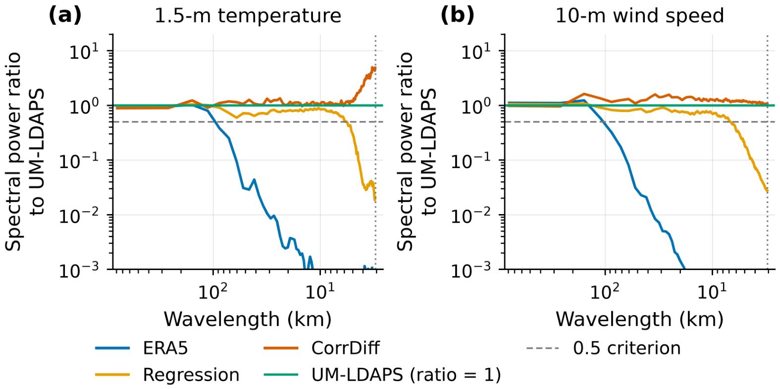
Scale-dependent variability of 1.5 m temperature and 10 m wind speed was analyzed using azimuthally averaged power spectra [16,17]. Separately from the South Korean land evaluation domain, the spectral analysis used a rectangular domain of 256 × 256 grid points (approximately 392 × 392 km) centered at 36.370° N, 127.831° E. For the field at each time, the linear spatial trend was removed based on the method of Errico [18], a two-dimensional Hann window was applied, and the azimuthally averaged power spectrum was computed; the spectra were then averaged over the entire test period. The relative magnitude of scale-dependent variability was evaluated using the spectral power ratio, defined as the time-mean spectrum of each dataset divided by the time-mean spectrum of the target.

Wavelengths were calculated using the mean grid spacing of 1.533 km derived from the latitudes and longitudes of the analysis domain, and the corresponding Nyquist wavelength is 3.07 km. Following the criterion used by Assouline et al. [12], the shortest wavelength at which the spectral power ratio was 0.5 or greater was determined. When this condition was satisfied down to the Nyquist wavelength, the criterion was regarded as met down to 3.07 km, the shortest wavelength that can be analyzed.

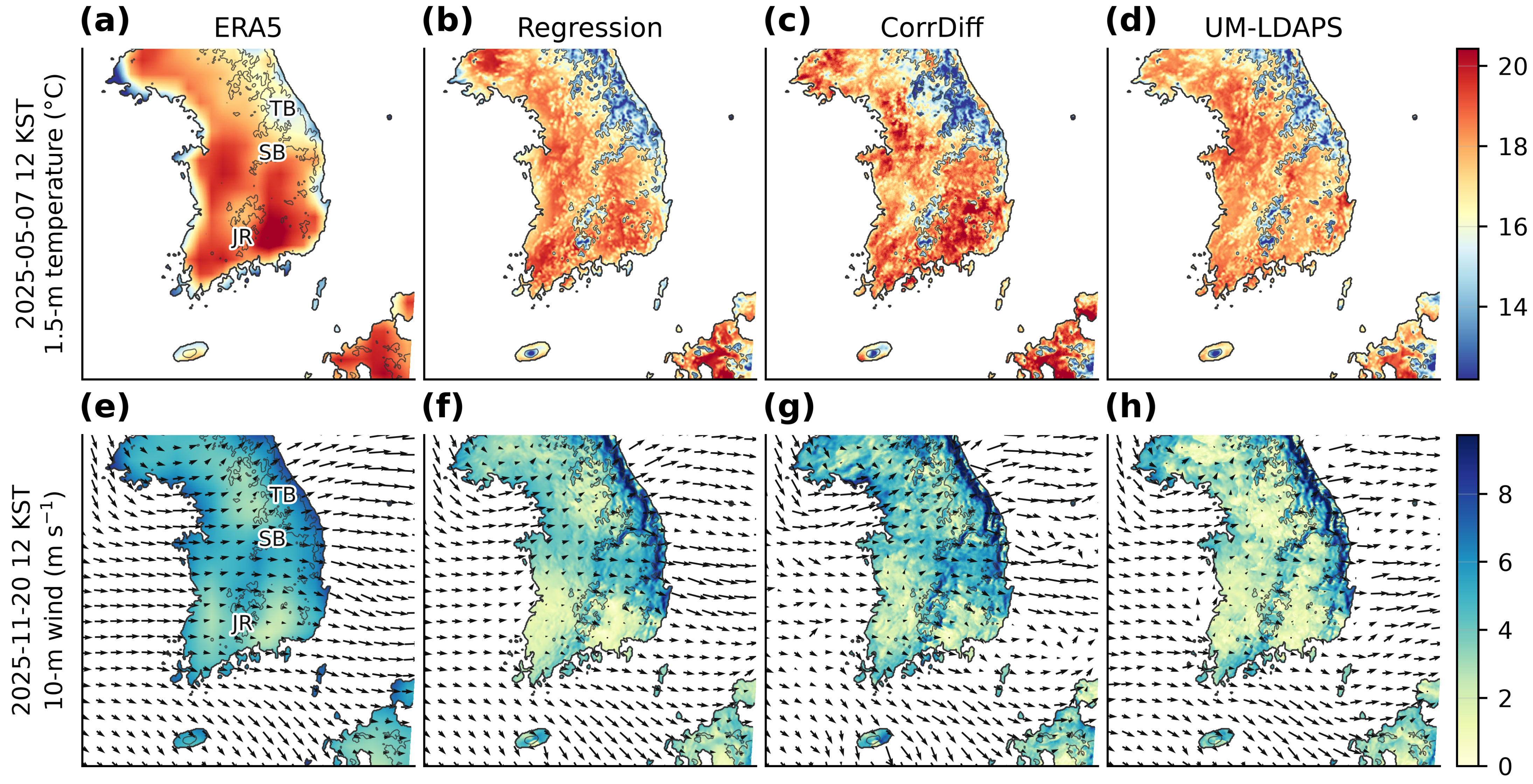
Changes in spatial structure associated with the regression and diffusion stages were compared using temperature and wind cases. The cases were selected by considering the ERA5 synoptic flow and the UM-LDAPS fields during the test period, and times are given in Korea Standard Time (KST; UTC+9). For temperature, 12 KST on 7 May 2025, when the low-level synoptic flow was weak, was selected; for wind, 12 KST on 20 November 2025, when westerly flow across the Taebaek Range was pronounced, was selected.

For each case, the spatial distributions of ERA5, Regression, CorrDiff, and UM-LDAPS were compared, and the temperature distribution width was defined as the difference between the 99th and 1st percentiles (p99 − p01).

Separately from the individual cases, low-temperature, high-temperature, and strong-wind events over the entire test period were evaluated in terms of detection, event frequency, and agreement in threshold exceedance, together with conditional errors. The temperature thresholds were determined from the target 1.5 m temperature distribution over the evaluation domain and the entire test period. Low-temperature events were defined as temperatures at or below the 5th and 1st percentiles (−5.12 and −10.43 °C, respectively), and high-temperature events were defined as temperatures at or above the 95th and 99th percentiles (28.60 and 32.23 °C, respectively). Strong-wind events were defined as 10 m wind speeds of 10 and 12 m s⁻¹ or greater. The same thresholds were applied to ERA5, Regression, and CorrDiff.

Over all grid point–time pairs in the evaluation domain and test period, the number of cases in which both the target and the dataset satisfied the condition was counted as hits (H). The numbers of cases in which only the target or only the dataset satisfied the condition were counted as misses (M) and false alarms (F), respectively. From these counts, the probability of detection (POD), frequency bias index (FBI), and critical success index (CSI) were calculated [19]:

$$\mathrm{POD}={\displaystyle \frac{H}{H+M}},\mathrm{FBI}={\displaystyle \frac{H+F}{H+M}},\mathrm{CSI}={\displaystyle \frac{H}{H+M+F}}.$$

POD is the fraction of grid point–time pairs with the event in the target at which the event also occurred in the dataset. FBI is the ratio of the event frequency in the dataset to that in the target, and a value of 1 indicates equal frequencies. CSI is the fraction of all grid point–time pairs with the event in the target or the dataset at which the event occurred in both. Conditional errors were computed on a fixed sample consisting only of the grid point–time pairs at which the event occurred in the target, so that the three datasets were compared on the same sample regardless of whether each dataset satisfied the condition. For low- and high-temperature events, the RMSE and bias of 1.5 m temperature were calculated; for strong-wind events, the RMSVE of 10 m wind and the bias of 10 m wind speed were calculated.

The ERA5-trained system was applied to AIFS medium-range forecast fields to evaluate the characteristics of temperature downscaling during the July 2026 heatwave case. AIFS forecast fields initialized at 00 and 12 UTC were bilinearly interpolated onto the 1.5 km target grid, and Regression and CorrDiff were then produced using the models selected in Section 2.2 and the static inputs used in training. The case period extended from 00 KST on 21 July to 00 KST on 28 July 2026, and the verification valid times were 03, 09, 15, and 21 KST each day. From the +6–288 h forecasts (at 6 h intervals) produced from a total of 31 initialization times between 00 UTC on 12 July and 00 UTC on 27 July 2026, we used those valid at the verification times within this period. Lead times were divided into short lead times (+6–120 h) and medium lead times (+126–288 h).

Hourly ASOS station observations were used as the observational data. Two conditions were applied to the hourly observations of all 97 ASOS stations: at least one day with a daily maximum temperature of 33 °C or higher during the case period, and accumulated precipitation of less than 10 mm over the same period. The 47 stations that met both conditions were used for the heatwave-focused quantitative evaluation. Daily maximum temperatures were derived from all hourly data for each day. Model values were taken from the grid point nearest to each station, and the height difference between the AIFS 2 m temperature and the Regression and CorrDiff 1.5 m temperatures was not adjusted.

A forecast sample was defined as a combination of (initialization time, lead time, valid time); forecasts with the same valid time but different initialization times were treated as separate samples. Because independence between samples could not be ensured, significance tests were not performed. The same-time spatial correlation was calculated for each forecast sample as the Pearson correlation coefficient between the forecast and observed values across the evaluation stations, and the across-station spatial variability was calculated as the standard deviation of temperature across stations for each dataset. For each lead-time range, the distribution and mean of the spatial correlation and the mean of the spatial variability are presented. The bias, RMSE, and POD, FBI, and CSI for temperatures ≥33 °C were calculated by pooling all forecast samples and evaluation stations within each lead-time range.

For the representative case, the spatial distributions and the temperature distribution width (p99 − p01) over land grid points were compared. The lead-time dependence of the temperature errors was evaluated by grouping the +6–288 h forecasts into twelve 24 h lead-time ranges (D1 = +6–24 h to D12 = +270–288 h), each containing four lead times. The lead-time-dependent evaluation was conducted using all 97 ASOS stations. The period of highest observed intensity was determined from the observations alone: the 90th percentile of the observed temperature across the 47 stations was computed at 15 KST on each day of the case period, and the three consecutive days with the highest mean of these daily values were selected, with the earlier start date taken in the event of a tie.

Generative AI tools were used for translation, language editing, and manuscript preparation and to assist in writing and revising code for data processing, the computation of evaluation metrics, and figure generation (see Acknowledgments). All AI-assisted code and text were reviewed, tested, and revised by the authors, who executed the code, verified the results, and are responsible for the analyses, the interpretation of the results, and the final content of the manuscript.

3. Results

3.1. Deterministic Downscaling Performance by Stage

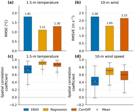
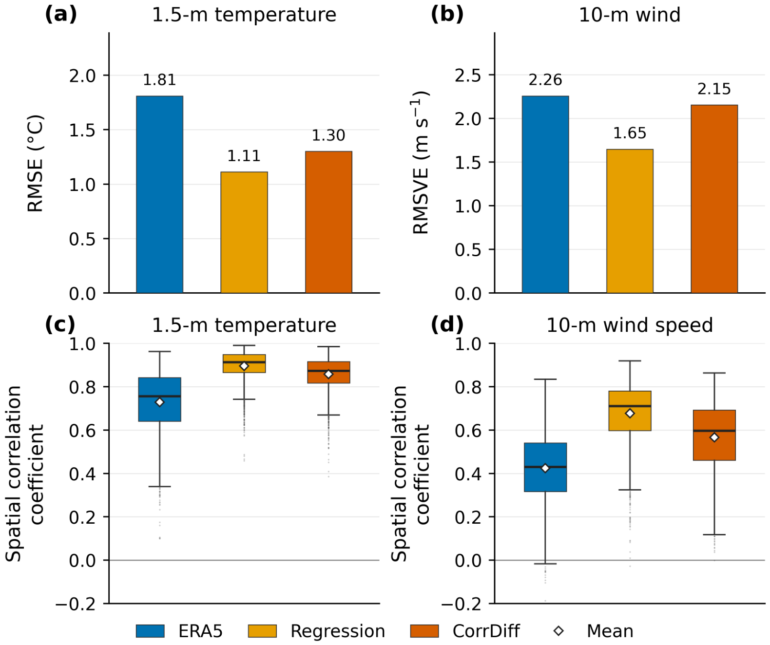
The deterministic errors and same-time spatial correlations of ERA5, Regression, and CorrDiff were compared against the UM-LDAPS target (Figure 3).

Figure 3. Deterministic performance of ERA5, Regression, and CorrDiff against UM-LDAPS over 40,873 South Korean land grid points during 1 March 2025–28 February 2026 (2920 times at 3 h intervals). (a) Temperature RMSE, (b) wind RMSVE, and same-time spatial correlations for (c) temperature and (d) wind speed. ERA5 temperature is at 2 m; Regression, CorrDiff, and UM-LDAPS temperatures are at 1.5 m. Wind is evaluated at 10 m. In (c,d), boxes span the interquartile range, central lines mark medians, whiskers extend to the most extreme values within 1.5 interquartile ranges of the box, dots denote outliers, and white diamonds indicate means.

The temperature RMSE decreased from 1.81 °C for ERA5 to 1.11 °C for Regression and then increased to 1.30 °C for CorrDiff. The 10 m wind RMSVE likewise decreased from 2.26 to 1.65 m s⁻¹ and then increased to 2.15 m s⁻¹ (Figure 3a,b).

The mean same-time spatial correlations of ERA5, Regression, and CorrDiff were 0.73, 0.90, and 0.86, respectively, for temperature and 0.42, 0.68, and 0.57, respectively, for 10 m wind speed; for both variables, Regression had the highest values (Figure 3c,d). At the regression stage, the RMSE and RMSVE decreased and the spatial correlation increased.

The temperature biases of ERA5, Regression, and CorrDiff were +0.83, −0.34, and +0.04 °C, respectively, and the 10 m wind speed biases were +0.08, −0.32, and +0.05 m s⁻¹, respectively. CorrDiff had the smallest absolute bias for both variables, but its RMSE and RMSVE were larger and its spatial correlations were lower than those of Regression.

3.2. Characteristics of the Downscaled Fields from the Regression Stage

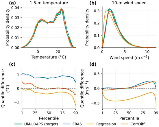
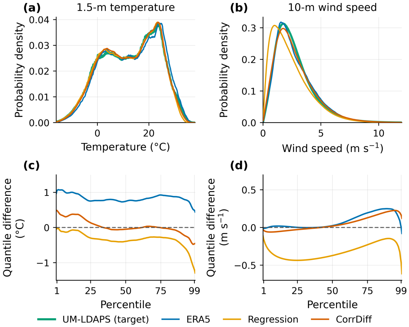
To examine whether the decreases in RMSE and RMSVE and the increase in spatial correlation at the regression stage were accompanied by closer agreement with the target in value distributions and scale-dependent variability, the temperature and wind speed distributions and the spectral power of ERA5 and Regression were compared with those of the target (Figure 4 and Figure 5).

Figure 4. Distributions of temperature and 10 m wind speed over South Korean land (40,873 grid points; 1 March 2025–28 February 2026; 2920 times at 3 h intervals). (a,b) Probability densities and (c,d) quantile differences (dataset − UM-LDAPS) for (a,c) temperature and (b,d) wind speed. Quantile differences cover the 0.5–99.5 percentile range. ERA5 temperature is at 2 m; Regression, CorrDiff, and UM-LDAPS temperatures are at 1.5 m. The wind speed axis in (b) is shown up to 12 m s⁻¹, and the dashed lines in (c,d) mark zero difference.

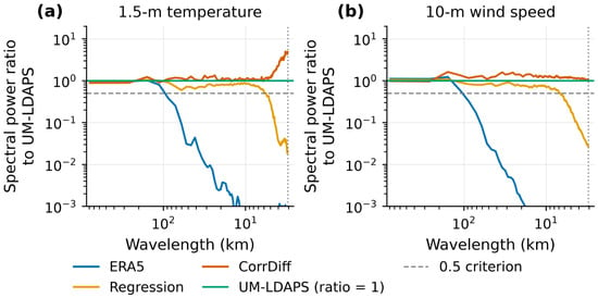
Figure 5. Spectral power ratio to UM-LDAPS for (a) temperature and (b) 10 m wind speed, calculated from azimuthally averaged spectra over a 256 × 256 grid-point domain centered on South Korea and averaged over all 2920 times at 3 h intervals during the test period. ERA5 temperature is at 2 m; Regression, CorrDiff, and UM-LDAPS temperatures are at 1.5 m. The UM-LDAPS reference corresponds to a ratio of 1, the horizontal dashed line marks a ratio of 0.5, and the vertical dotted line marks the Nyquist wavelength of 3.07 km.

For temperature, the ERA5 quantiles were higher than those of the target over the entire evaluated range of the 0.5–99.5 percentiles (Figure 4c). The quantile differences from the target were +1.06 °C at p01, +0.75 °C at p50, and +0.49 °C at p99 for ERA5 and −0.03, −0.39, and −1.20 °C, respectively, for Regression. After the regression stage, the absolute differences decreased at p01 and p50 but increased at p99; thus, in contrast to the decrease in the overall temperature RMSE, the difference from the target became larger in the upper quantiles.

For 10 m wind speed, the differences from the target in the lower and middle quantiles were small for ERA5 (0.00 m s⁻¹ at p25 and +0.02 m s⁻¹ at p50), whereas those for Regression were −0.44 and −0.37 m s⁻¹, respectively, indicating lower values than the target (Figure 4d). The frequency of wind speeds below 1 m s⁻¹ was also higher for Regression (21.6%) than for the target (10.2%) and ERA5 (9.8%); thus, in contrast to the decrease in the wind vector error, the frequency of wind speeds below 1 m s⁻¹ exceeded that of the target.

In the short-wavelength range, the spectral power of Regression was greater than that of ERA5 (Figure 5). The shortest wavelengths at which the power ratio to the target was 0.5 or greater were 5.73 km for temperature and 6.83 km for wind speed. At shorter wavelengths, the power ratio decreased, reaching 0.02 for temperature and 0.03 for wind speed at the Nyquist wavelength of 3.07 km. The regression stage increased the variability at short wavelengths, which was weak in ERA5, but the power at the shortest analyzed wavelength was far below that of the target.

Despite the reduced RMSE and RMSVE and increased spatial correlation after the regression stage, differences from the target remained in the value distributions and in the variability at short wavelengths.

3.3. Changes in the Downscaled Fields After the Diffusion Stage

To examine the changes associated with the diffusion stage, the temperature and wind speed distributions and the spectral power of Regression and CorrDiff were compared (Figure 4 and Figure 5).

For temperature, the changes after the diffusion stage differed among quantiles (Figure 4c). The absolute difference from the target increased at p01, from −0.03 °C for Regression to +0.48 °C for CorrDiff, whereas the difference moved closer to zero at p50 (from −0.39 to −0.05 °C) and at p99 (from −1.20 to −0.46 °C).

For 10 m wind speed, the absolute differences in the lower and middle quantiles became smaller than those of Regression, changing from −0.44 to −0.03 m s⁻¹ at p25 and from −0.37 to +0.02 m s⁻¹ at p50 (Figure 4d). The frequency of wind speeds below 1 m s⁻¹ also decreased from 21.6% for Regression to 11.4% for CorrDiff, closer to the target value of 10.2%. In the upper quantiles, however, CorrDiff was slightly higher than the target.

After the diffusion stage, the spectral power at short wavelengths increased (Figure 5). For both temperature and wind speed, the power ratio of CorrDiff to the target remained at or above 0.5 down to the Nyquist wavelength of 3.07 km, where the ratio was 4.84 for temperature and 1.07 for wind speed. At the Nyquist wavelength, the temperature power greatly exceeded that of the target, whereas the wind speed power was close to but slightly higher than that of the target.

3.4. Changes in Spatial Structure by Downscaling Stage

To examine how the stage-dependent characteristics appeared in the spatial fields at individual times, the spatial distributions of ERA5, Regression, CorrDiff, and UM-LDAPS were compared for the temperature and wind cases selected in Section 2.3 (Figure 6).

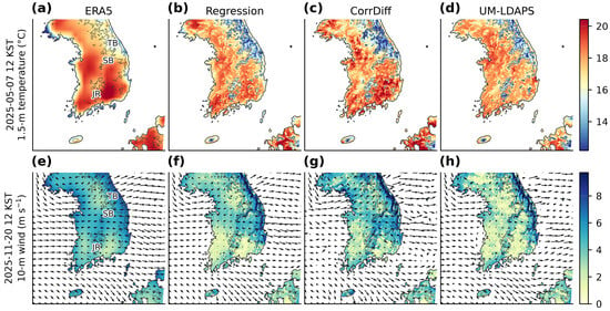
Figure 6. Spatial distributions of temperature and 10 m wind by downscaling stage. (a–d) Temperature at 12 KST on 7 May 2025 and (e–h) 10 m wind speed at 12 KST on 20 November 2025. Within each row, the columns show ERA5, Regression, CorrDiff, and UM-LDAPS. ERA5 temperature is at 2 m; Regression, CorrDiff, and UM-LDAPS temperatures are at 1.5 m. Grey contours indicate the 500 m model terrain elevation, and arrows show the 10 m wind vectors. TB, SB, and JR denote the Taebaek Range, the Sobaek Range, and Jirisan, respectively.

In the temperature case, the spatial distribution of ERA5 was relatively smooth, with a temperature distribution width (p99 − p01) of 7.20 °C (Figure 6a–d). In Regression, terrain-related spatial structures became more distinct, including lower temperatures than in the surroundings along the Taebaek and Sobaek Ranges, but the distribution width (7.23 °C) was similar to that of ERA5. In CorrDiff, both local temperature variations and the contrast between warmer and colder areas increased, and the distribution width (8.89 °C) was larger than those of Regression and the target (7.10 °C).

In the wind case, westerly flow across the Taebaek Range was present (Figure 6e–h). Regression showed a more distinct wind speed contrast between mountainous areas and lowlands than ERA5, similar to the spatial distribution of the target. In CorrDiff, wind speeds in the surrounding lowlands were higher, and this contrast was partly weakened. In the southern mountainous areas, wind direction and speed in Regression and CorrDiff varied locally with the terrain, and the same feature was also present in the target.

Thus, in the two selected cases, the diffusion stage did not uniformly strengthen the local contrasts in the regression output.

3.5. Evaluation of Low-Temperature, High-Temperature, and Strong-Wind Events

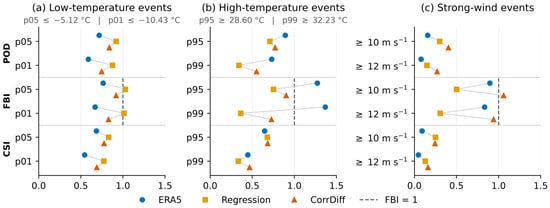
For low-temperature, high-temperature, and strong-wind events over the entire test period, POD, FBI, CSI, and conditional errors were compared. For low-temperature events, the thresholds were the p05 (−5.12 °C) and p01 (−10.43 °C) of the target 1.5 m temperature, with events defined at or below each threshold. For high-temperature events, the thresholds were the p95 (28.60 °C) and p99 (32.23 °C), with events defined at or above each threshold. Strong-wind events were defined using 10 m wind-speed thresholds of 10 and 12 m s⁻¹, with events defined at or above each threshold. Figure 7 shows the POD, FBI, and CSI of ERA5, Regression, and CorrDiff, and Table 2 shows the conditional errors over the grid point–time pairs at which each event occurred in the target.

Figure 7. POD, FBI, and CSI of ERA5, Regression, and CorrDiff for (a) low-temperature, (b) high-temperature, and (c) strong-wind events, evaluated against UM-LDAPS over all grid points and times in the South Korean land domain during the test period. Grey lines connect ERA5, Regression, and CorrDiff within each metric, and the dashed line marks FBI = 1.

Table 2. Conditional errors over the grid points and times at which each event occurred in UM-LDAPS: temperature RMSE and bias for low- and high-temperature events, and 10 m wind RMSVE and wind speed bias for strong-wind events. ERA5 temperature is at 2 m; Regression, CorrDiff, and UM-LDAPS temperatures are at 1.5 m.

Condition	Threshold	Metric (Unit)	Grid Points × Times	ERA5	Regression	CorrDiff
Low temperature	≤−5.12 °C	RMSE/bias (°C)	5,967,491	2.23/+1.40	0.94/+0.07	1.33/+0.62
Low temperature	≤−10.43 °C	RMSE/bias (°C)	1,193,498	2.52/+1.64	0.87/+0.16	1.31/+0.75
High temperature	≥28.60 °C	RMSE/bias (°C)	5,967,513	1.53/+0.14	1.57/−1.23	1.59/−0.77
High temperature	≥32.23 °C	RMSE/bias (°C)	1,193,550	1.53/−0.38	1.91/−1.65	1.69/−1.05
Strong wind	≥10 m s−1	RMSVE/bias (m s−1)	309,127	5.38/−4.06	3.48/−2.30	4.11/−2.06
Strong wind	≥12 m s−1	RMSVE/bias (m s−1)	62,223	6.52/−5.43	4.35/−3.22	4.99/−2.88

For low-temperature events, Regression had the highest POD and CSI, the FBI closest to 1, and the smallest conditional temperature errors at both thresholds (Figure 7a, Table 2). At p01, the POD values of ERA5, Regression, and CorrDiff were 0.59, 0.88, and 0.75, respectively; the CSI values were 0.54, 0.77, and 0.69; the conditional RMSEs were 2.52, 0.87, and 1.31 °C; and the conditional biases were +1.64, +0.16, and +0.75 °C. After the diffusion stage, POD and CSI for low-temperature events decreased, and the positive temperature bias and the conditional RMSE increased.

For high-temperature events, the effects of the diffusion stage differed by threshold (Figure 7b). At p95, the CSI values of ERA5, Regression, and CorrDiff were 0.65, 0.68, and 0.68, respectively, showing small differences, and the FBI values were 1.27, 0.75, and 0.90, respectively, with CorrDiff closer to 1 than Regression. From Regression to CorrDiff, however, the conditional RMSE increased slightly from 1.57 to 1.59 °C, whereas the absolute conditional bias decreased (from −1.23 to −0.77 °C) (Table 2). At p99, POD increased from 0.34 to 0.55, CSI increased from 0.33 to 0.47, and FBI moved closer to 1, i.e., from 0.36 to 0.73; the conditional RMSE decreased from 1.91 to 1.69 °C, and the conditional bias moved closer to zero, i.e., from −1.65 to −1.05 °C. Although the changes at p95 were not consistent across metrics, at p99, POD and CSI increased, the event frequency became closer to that of the target, and the conditional temperature errors decreased relative to Regression.

For strong-wind events, POD increased from Regression to CorrDiff, from 0.30 to 0.40 at ≥10 m s⁻¹ and from 0.15 to 0.27 at ≥12 m s⁻¹, and the FBI values of CorrDiff (1.06 and 0.94, respectively) were the closest to 1 (Figure 7c). In contrast, CSI decreased from 0.25 to 0.24 at ≥10 m s⁻¹ and increased from 0.13 to 0.16 at ≥12 m s⁻¹; the conditional RMSVE increased at both thresholds, whereas the absolute wind speed bias decreased (Table 2). After the diffusion stage, the strong-wind event frequency became closer to that of the target and the negative wind speed bias was alleviated, but the wind vector error at the grid point–time pairs where strong winds occurred in the target increased.

Thus, the effects of the diffusion stage differed by event type, threshold, and evaluation metric, and among the evaluated conditions, the most consistent improvement relative to Regression occurred for p99 high-temperature events.

3.6. Application to AIFS Medium-Range Forecasts

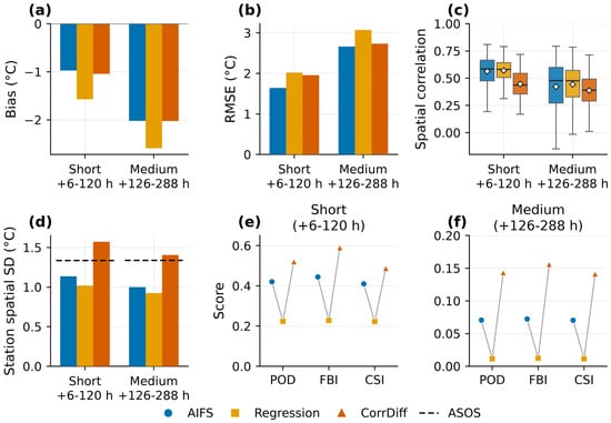
The ERA5-trained downscaling system was applied to AIFS forecast fields to produce 1.5 km medium-range forecast data, and the temperature downscaling characteristics during the July 2026 heatwave case were compared with ASOS observations. For the AIFS, Regression, and CorrDiff, temperature errors, spatial correlation, across-station spatial variability, and the occurrence of temperatures ≥33 °C were evaluated at short (+6–120 h) and medium (+126–288 h) lead times. Following the criteria in Section 2.3, forecasts from 31 initialization times were used, and the forecast–observation pairs at the 47 stations numbered 13,160 at short lead times and 16,450 at medium lead times, generating a total of 29,610 (Figure 8, Table 3).

Figure 8. Temperature verification of the AIFS, Regression, and CorrDiff at the 47 ASOS stations during the July 2026 heatwave: (a) bias, (b) RMSE, (c) same-time spatial correlation, and (d) spatial standard deviation across stations, both for short (+6–120 h) and medium (+126–288 h) lead times. Spatial statistics are calculated for each initialization–valid-time combination. Panel (d) shows mean spatial standard deviations, with the dashed line indicating the ASOS value. In (c), boxes span the interquartile range, central lines mark medians, whiskers extend to the most extreme values within 1.5 interquartile ranges of the box, and white diamonds indicate means. (e,f) POD, FBI, and CSI for temperatures ≥33 °C at short and medium lead times, respectively. Grey lines connect datasets within each metric. Panels (e,f) use different vertical scales. The AIFS temperature is at 2 m; Regression and CorrDiff temperatures are at 1.5 m.

Table 3. Verification results for the AIFS, Regression, and CorrDiff at the 47 ASOS stations during the July 2026 heatwave. Samples are station–forecast pairs. Spatial correlation and spatial variability are the means of the across-station Pearson correlation with observations and temperature standard deviation, respectively, calculated for each initialization–valid-time combination. POD, FBI, and CSI are for temperatures ≥33 °C.

Lead Time	Dataset	Samples	Bias (°C)	RMSE (°C)	Spatial Correlation	Spatial Variability (°C)	POD	FBI	CSI
+6–120 h	ASOS	—	—	—	—	1.34	—	—	—
	AIFS	13,160	−0.97	1.64	0.56	1.14	0.42	0.44	0.41
	Regression	13,160	−1.57	2.02	0.57	1.02	0.22	0.23	0.22
	CorrDiff	13,160	−1.04	1.96	0.45	1.57	0.52	0.59	0.49
+126–288 h	ASOS	—	—	—	—	1.34	—	—	—
	AIFS	16,450	−2.02	2.66	0.42	1.00	0.07	0.07	0.07
	Regression	16,450	−2.59	3.07	0.44	0.93	0.01	0.01	0.01
	CorrDiff	16,450	−2.03	2.73	0.39	1.40	0.14	0.16	0.14

For all three datasets, the negative temperature bias and the RMSE were larger and the same-time spatial correlation was lower at medium lead times than at short lead times, and the changes by downscaling stage were similar at the two lead-time ranges (Figure 8a–c). Compared with the AIFS, Regression had a larger absolute bias (short: −0.97 →−1.57 °C; medium: −2.02 →−2.59 °C) and a larger RMSE (short: 1.64 → 2.02 °C; medium: 2.66 → 3.07 °C). For CorrDiff, the magnitude of the bias (−1.04 °C at short and −2.03 °C at medium lead times) and the RMSE (1.96 and 2.73 °C, respectively) were smaller than those of Regression, but the RMSE was larger than that of the AIFS at both lead-time ranges.

The mean same-time spatial correlations were 0.56 and 0.42 for the AIFS at short and medium lead times, respectively; 0.57 and 0.44 for Regression; and 0.45 and 0.39 for CorrDiff. Regression had larger temperature errors than the AIFS but slightly higher spatial correlations. In contrast, CorrDiff had smaller temperature errors than Regression but lower spatial correlations. Thus, in this case, the decrease in temperature errors was not accompanied by closer agreement with the observed spatial distribution of temperature.

The across-station spatial variability decreased in Regression and increased in CorrDiff (Figure 8d). The mean across-station standard deviation of observed temperature was 1.34 °C at both lead-time ranges, whereas those of the AIFS, Regression, and CorrDiff were 1.14, 1.02, and 1.57 °C, respectively, at short lead times and 1.00, 0.93, and 1.40 °C, respectively, at medium lead times. The AIFS and Regression showed smaller spatial variability than the observations at both lead-time ranges, whereas CorrDiff showed larger values. At medium lead times, the spatial variability for CorrDiff was the closest to the observations among the three datasets, but its spatial correlation was the lowest.

The verification of temperatures ≥33 °C also differed by downscaling stage (Figure 8e,f). At short lead times, the POD values of the AIFS, Regression, and CorrDiff were 0.42, 0.22, and 0.52, respectively; the FBI values were 0.44, 0.23, and 0.59; and the CSI values were 0.41, 0.22, and 0.49. At medium lead times, POD (0.07, 0.01, and 0.14), FBI (0.07, 0.01, and 0.16), and CSI (0.07, 0.01, and 0.14) showed the same order. At both lead-time ranges, Regression had lower POD and CSI than the AIFS, and its tendency to underpredict the frequency of high-temperature occurrence relative to the observations became stronger. CorrDiff had the highest POD and CSI among the three datasets and the FBI closest to 1. However, the FBI of CorrDiff at medium lead times was only 0.16, and the frequency of high-temperature occurrence remained much lower than observed.

To examine the period of highest observed intensity separately, 25–27 July 2026 was identified, from the observations alone, as the three consecutive days with the highest three-day mean of the 90th percentile of observed temperatures across the 47 stations at 15 KST. Of the 31 initialization times, 29 had forecast windows covering these three days; over their four verification times per day they provided 13,536 matched station–forecast pairs per dataset, the pooled temperature RMSE was 2.40 °C for the AIFS, 2.81 °C for Regression, and 2.53 °C for CorrDiff, and the biases were −1.70, −2.31, and −1.78 °C. For all three datasets, both the RMSE and the magnitude of the bias were larger during this period than over the case period as a whole, and the RMSE of CorrDiff remained smaller than that of Regression and larger than that of the AIFS.

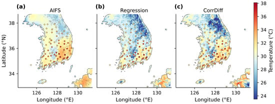
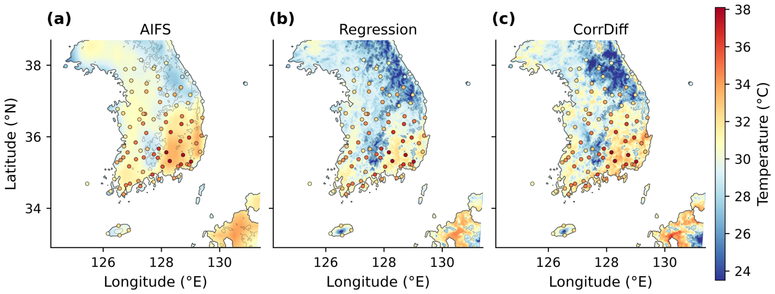
As a representative case at medium lead times, the spatial distributions of the +150 h forecast were compared (Figure 9). The temperature distribution of the AIFS was relatively smooth, terrain-related spatial structures became more distinct in Regression, and temperature variations at smaller spatial scales appeared in CorrDiff. The temperature contrast between the relatively warm zone along the Yeongdong coast and the adjacent mountainous areas also became more distinct in the order of the AIFS, Regression, and CorrDiff. The temperature distribution width (p99 − p01) over land grid points in the displayed domain increased from 6.29 °C for the AIFS to 9.98 °C for Regression and 11.68 °C for CorrDiff. However, closer agreement with the observations cannot be concluded from these changes alone.

Figure 9. Temperature fields from (a) the AIFS, (b) Regression, and (c) CorrDiff at +150 h, with an initialization time of 00 UTC on 20 July 2026 and a valid time of 15 KST on 26 July 2026. The AIFS temperature is at 2 m; Regression and CorrDiff temperatures are at 1.5 m. Circles show available ASOS observations from the 97-station network, using the same color scale as the fields; quantitative verification uses the selected 47 stations. Grey contours indicate the 500 m model terrain elevation.

Relative to Regression, CorrDiff had smaller temperature errors and higher POD and CSI for high-temperature occurrence but lower spatial correlation, and its RMSE was larger than that of the AIFS. These results characterize the application to a single heatwave case at the 47 selected stations; the dependence of the temperature errors on lead time is examined at all 97 stations below (Figure 10).

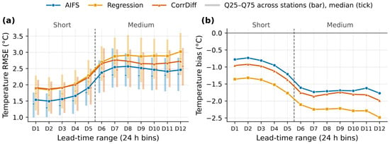
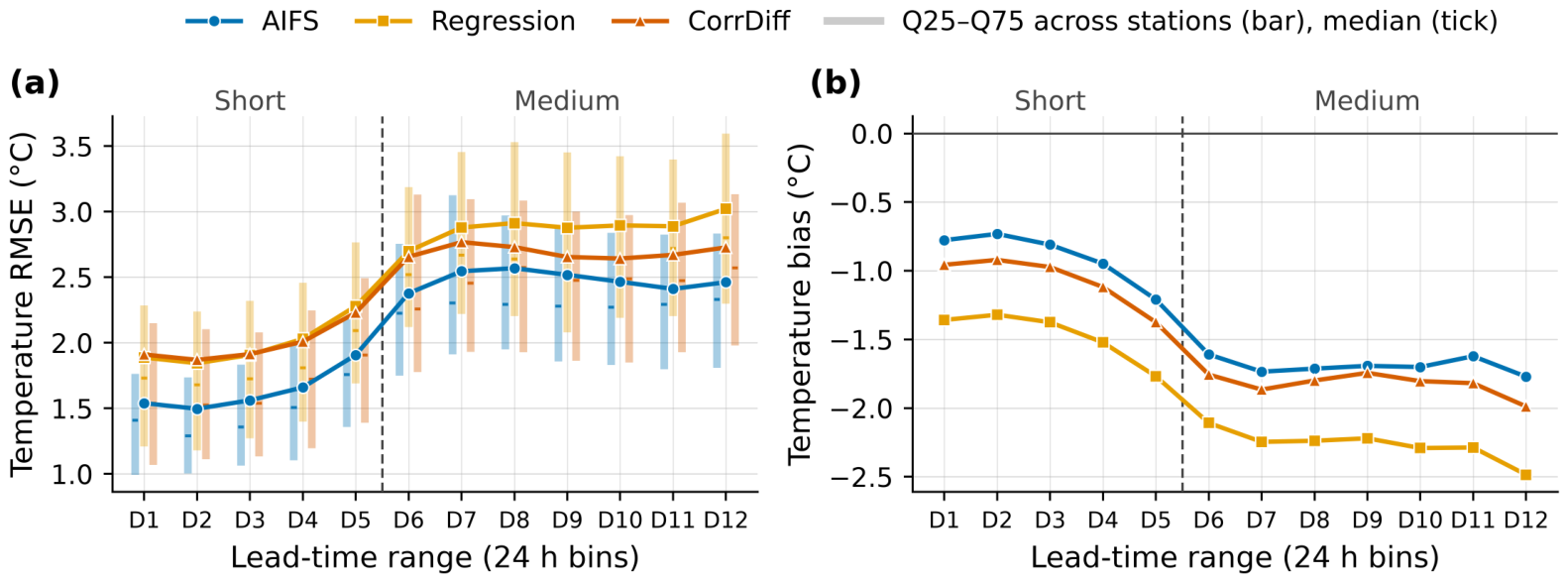
Figure 10. Temperature (a) RMSE and (b) bias of the AIFS, Regression, and CorrDiff at the 97 ASOS stations during the July 2026 heatwave, shown for twelve 24 h lead-time ranges (D1 = +6–24 h to D12 = +270–288 h). The three datasets are verified on identical station–initialization–lead–valid-time samples (61,110 station–forecast pairs per dataset). Solid lines are the pooled RMSE and bias over all matched samples; in (a), the vertical bars give the interquartile range (Q25–Q75) of the per-station RMSE values and the horizontal ticks their median, offset horizontally for legibility. The bars show the spread across stations and are not confidence intervals. Bias is the forecast minus the observation. The dashed line separates the short (D1–D5) and medium (D6–D12) lead-time ranges. Unlike Figure 8 and Table 3, which use the 47 selected stations, this figure uses all 97 stations. The AIFS temperature is at 2 m; Regression and CorrDiff temperatures are at 1.5 m.

Figure 10 resolves the lead-time dependence of the temperature errors into twelve 24 h ranges. Because this breakdown describes the general behavior of the errors with lead time rather than the heatwave itself, it uses all 97 ASOS stations, whereas Figure 8 and Table 3 use the subset of 47 stations defined in Section 2.3; the samples therefore differ and values from the two figures are not compared directly. For all three datasets, the RMSE increased and the negative bias deepened with lead time: from D1 to D12, the RMSE increased from 1.54 to 2.46 °C for the AIFS, from 1.89 to 3.02 °C for Regression, and from 1.91 to 2.73 °C for CorrDiff, and the bias changed from −0.78, −1.36, and −0.96 °C to −1.77, −2.48, and −1.99 °C, respectively. The RMSE of the AIFS was lower than that of CorrDiff in all twelve ranges. Relative to Regression, CorrDiff had a lower RMSE in nine of the twelve ranges and a smaller absolute bias in all twelve; the three ranges without a lower RMSE were D1–D3, where the difference was within 0.03 °C.

4. Discussion

4.1. Downscaling Characteristics of the Regression and Diffusion Stages

In the ERA5-input evaluation, the regression stage reduced deterministic errors and increased spatial correlation, whereas the diffusion stage increased spatial variability but resulted in larger deterministic errors and lower spatial correlation than the regression output. This difference can be interpreted in relation to the two-stage structure of CorrDiff. In CorrDiff, the regression stage predicts high-resolution fields, and the diffusion stage learns and generates the residual between the regression prediction and the target [3]. Mardani et al. [3] explained that the two stages are trained with different objective functions and that deterministic errors after the diffusion stage can be larger than those after the regression stage; the same pattern was found in the ERA5-input evaluation of this study. This suggests that the two stages exhibit different downscaling characteristics. Therefore, evaluating the diffusion stage only in terms of deterministic errors does not fully reflect the added spatial variability and the changes in distribution characteristics.

While reducing deterministic errors, the regression stage also produced terrain-related spatial structures that were not fully represented in ERA5. Mardani et al. [3] explained that terrain effects not represented in low-resolution inputs are important for temperature downscaling and can be learned deterministically from static inputs. In the temperature case of this study, the spatial structures of the regression output along the Taebaek and Sobaek Ranges are qualitatively consistent with this explanation and show that these terrain-related spatial structures were already present in the regression output before the diffusion stage. However, because no comparative experiments with different static-input configurations were conducted, the individual contributions of terrain elevation and the land–sea mask to the observed spatial structures cannot be separated.

The diffusion stage increased the spectral power in the short-wavelength range, where the regression output had lower power than the target. Whereas the regression output had much lower power than the target at the shortest wavelengths, CorrDiff maintained a power ratio to the target at or above 0.5 down to the Nyquist wavelength for both temperature and wind speed. Tomasi et al. [8], who learned residuals with a diffusion model, reported that small-scale structures were generated through the diffusion stage, and in the present 1.5 km downscaling over the Korean Peninsula, short-wavelength variability also increased after the diffusion stage. However, the degree to which the power approached the target differed between the variables. Near the Nyquist wavelength, the wind speed power was comparable to that of the target, whereas the temperature power greatly exceeded it. That is, the spatial variability added by the diffusion stage appeared not only as a supplement to variability that had been lower than in the target but also as variability in excess of the target; therefore, an increase in spatial variability itself cannot be equated with closer agreement with the target.

Value distributions and spectral power represent statistical properties of spatial variability but do not evaluate whether local spatial structures were generated at the same locations as in the target at individual times. After the diffusion stage, the middle and upper temperature quantiles and the frequency of wind speeds below 1 m s⁻¹ became closer to the target, whereas the same-time spatial correlation decreased. In this study, even when one aspect—statistical similarity or agreement in spatial placement—became closer to the target, the other did not necessarily improve simultaneously. Therefore, the results of generative downscaling should be evaluated by distinguishing statistical similarity from spatial agreement.

4.2. Effects of the Diffusion Stage Depending on Event Type and Intensity

The effects of the diffusion stage differed by event type and threshold. For low-temperature events, the regression output had better POD, CSI, and conditional errors at both thresholds. For p99 high-temperature events, POD and CSI increased after the diffusion stage, FBI moved closer to 1, and conditional errors decreased, representing the most consistent improvement among the evaluated conditions. This contrast is qualitatively in the same direction as the changes in the temperature distribution after the diffusion stage, in which the middle and upper parts became closer to the target and the lower part became higher than the target. However, the quantile differences are statistics comparing the entire temperature distributions, whereas the conditional errors consider only the grid point–time pairs at which each event occurred in the target. Although the two results show related tendencies, they do not evaluate the same information; therefore, the changes in the distribution cannot be regarded as the cause of the changes in conditional errors or CSI.

For strong-wind events, the directions of change after the diffusion stage differed among metrics. POD increased at both thresholds, FBI moved closer to 1, and the absolute wind speed bias decreased, but the change in CSI was not consistent between thresholds, and the conditional RMSVE increased. The increases in POD and the closer agreement of event frequency with the target after the diffusion stage were not accompanied by consistent improvement in CSI or by reduced wind vector error.

Previous studies have also reported that the effects of the diffusion stage vary across variables and ranges of meteorological fields. In Mardani et al. [3], the contribution of the diffusion component differed between the overall temperature and wind speed distributions and the strong wind speeds in a typhoon case, and Tomasi et al. [8] reported greater difficulty in reproducing the wind speed distribution than the temperature distribution. In this study as well, the effects of the diffusion stage differed among low-temperature, high-temperature, and strong-wind events, and for temperature, they also differed between the low and high sides of the distribution and between thresholds. In particular, the consistent improvement for p99 high-temperature events indicates a possible contribution of the diffusion stage to representing strong high-temperature conditions. However, this result was obtained for a 1-year test period, the UM-LDAPS target, and the thresholds defined in this study. The contribution of generative downscaling may thus not be evident in the overall-mean deterministic performance and should be examined through evaluations that distinguish event type and intensity.

4.3. Characteristics of the Application to AIFS Medium-Range Forecasts

The ERA5-trained system was applied to AIFS forecast fields without additional training or correction and produced 1.5 km downscaled data through +288 h, and the representative spatial field showed terrain-related regional temperature distributions. This demonstrates that a downscaling system trained on reanalysis data can be linked directly to global AI forecast fields to produce 1.5 km medium-range forecast data over the Korean Peninsula. However, the ability to produce high-resolution data and an improvement in forecast performance against observations are separate issues.

The change in errors at the regression stage differed between the two evaluations. In the ERA5-input evaluation, the regression output had smaller deterministic errors than its input, whereas in the AIFS heatwave case, it had larger temperature errors than the AIFS. In relation to these differences, the differences between ERA5 used for training and the AIFS used for application should be considered. Differences between the data used for training and for application have also been addressed in related forecasting studies. Oh et al. [20] reported that the forecast performance of a machine-learning-based global weather prediction model differed depending on whether ERA5 or operational analyses were used as initial conditions, and Taccari et al. [21] presented an approach for hydrological forecasting in which a model pretrained on reanalysis data was fine-tuned on operational forecast data to account for differences between the two. Although these two studies differ from the present study in their applications, they support the need to examine differences between the training data and the input data used in actual application. However, the two evaluations in this study differ not only in their input data but also in their reference data (1 year of UM-LDAPS grid fields versus the selected stations for a single heatwave case), evaluation periods, and spatial samples, and the differences in input-data distributions between ERA5 and the AIFS were not analyzed directly. Therefore, the differences between the two evaluations cannot be attributed to differences in the input-data distributions of ERA5 and the AIFS, and whether the downscaling characteristics identified with reanalysis inputs are retained with forecast inputs requires a separate diagnosis that includes a comparison of the distributions of the two input datasets.

In the AIFS heatwave case, the diffusion stage reduced temperature errors and alleviated the underprediction of high-temperature occurrence relative to the regression output, and the POD and CSI of CorrDiff were higher than those of the AIFS. In contrast, its spatial correlation was lower than that of the regression output, and its RMSE was not improved relative to the original AIFS forecasts. In particular, the across-station spatial variability for CorrDiff was larger than that of the observations at short lead times and closest to the observations at medium lead times, but its spatial correlation was the lowest of the three datasets at both lead-time ranges. This shows that bringing the magnitude of temperature differences among stations closer to the observations does not necessarily imply better reproduction of the observed spatial arrangement of high and low temperatures. Although the reference data and evaluation designs differ, spatial variability and agreement in spatial placement did not necessarily improve together in the target-based evaluation either. In addition, at medium lead times, the frequency of temperatures ≥33 °C remained much lower than observed even in CorrDiff, and much of the high-temperature underprediction in the input forecast fields remained after downscaling. Because these results are based on a single heatwave case and 47 selected stations, further verification under other synoptic conditions and in other seasons is needed. An exploratory comparison of peak-intensity dates across the 24 initializations whose forecast windows contained the observed peak date did not indicate a consistent reduction in peak-date error for CorrDiff relative to the AIFS. This comparison is limited because many predicted peaks fell at the edges of the forecast window, because the result depends on the station set and the intensity metric used, and because the 6 h verification interval does not determine the time of day at which the daily maximum temperature occurs. Nevertheless, this case showed that when the ERA5-trained downscaling system was applied directly to the AIFS medium-range forecasts, the diffusion stage yielded better high-temperature detection than both the regression output and the AIFS, whereas it did not exceed the performance of the input forecast fields in temperature errors and spatial correlation. The applicability of the downscaled data should therefore be evaluated by considering the detailed spatial structure together with lead-time-dependent temperature errors, spatial correlation, and high-temperature detection performance.

4.4. Limitations and Future Work

In this study, only a single CorrDiff generated field was evaluated for each input time. The presented results therefore characterize single generated fields, and the variability among outputs generated from the same input, the ensemble spread, and the reliability of probabilistic forecasts were not evaluated. Because the diffusion stage generates downscaled fields stochastically, evaluation of a single generated field is insufficient to fully assess the probabilistic characteristics provided by the diffusion stage. Future studies should analyze the relationship between the spread of generated outputs and actual errors through ensemble inference and verify the reliability of probabilistic forecasts.

The characteristics of the training target and the evaluation references also limit the scope of interpretation. Because UM-LDAPS is a numerical model analysis rather than observations, closer agreement with the target does not imply greater accuracy with respect to the real atmosphere. Evaluation using ASOS stations directly assesses performance against observations, but it includes differences in spatial representativeness between gridded data and station observations, and the height difference between the 2 m temperature of ERA5 and the AIFS and the 1.5 m temperature of Regression, CorrDiff, and UM-LDAPS was not adjusted. In addition, the grid-based and station-based evaluations differ in evaluation period and spatial sample, which limits direct comparison of the two results. The scope of the evaluation is also limited to temperature and wind, a 1-year grid-based evaluation period, and a single AIFS heatwave case, and further verification for various seasons and weather phenomena is needed. Because the quantitative evaluation was restricted to South Korea, the reported performance should not be generalized to the entire Korean Peninsula. Future work should quantitatively assess differences between the ERA5 training inputs and AIFS forecast inputs and examine their potential effects on downscaling performance, with model adaptation or fine-tuning considered if warranted by the results.

Terrain elevation and the land–sea mask were used as static inputs, and although terrain-related spatial structures appeared in individual cases, the contribution of each static input was not evaluated separately. A study that statistically downscaled wind resource maps for South Korea reported reduced errors when terrain data at multiple resolutions were added [22]; however, because that study targeted climatological wind speed distributions, the same effect cannot be assumed for the downscaling of meteorological fields at individual times. The effects of additional static information, such as terrain data at multiple resolutions, land cover, and vegetation, need to be verified through comparative experiments. Because increased spatial variability in this study was not necessarily accompanied by reduced errors or improved spatial agreement, the effects of additional static information should also be evaluated based on improvements in errors relative to observations and in event-specific performance rather than on spatial variability itself.

5. Conclusions

In this study, we developed a 1.5 km CorrDiff downscaling system to produce high-resolution medium-range forecast data for the Korean Peninsula. We evaluated the characteristics of the regression and diffusion stages of the system trained with ERA5 and UM-LDAPS analyses and applied the system to AIFS forecast fields to produce high-resolution data through +288 h. In the ERA5-input evaluation, the regression stage reduced deterministic errors and increased spatial correlation relative to ERA5, and the diffusion stage increased spatial variability relative to the regression output. For p99 high-temperature events, POD and CSI increased and conditional errors decreased after the diffusion stage, representing the most consistent improvement relative to the regression output among the evaluated conditions; in contrast, the regression output performed better for low-temperature events, and the effects of the diffusion stage on strong-wind events differed across metrics. In addition, the increase in spatial variability after the diffusion stage was not consistently accompanied by improved spatial agreement.

In the AIFS heatwave case at the 47 selected stations, CorrDiff had smaller temperature errors and alleviated the underprediction of high-temperature occurrence relative to Regression, and its POD and CSI were higher than those of the AIFS. However, its station temperature RMSE and spatial correlation were not improved relative to the AIFS. This study applied CorrDiff trained on reanalysis data to the regional downscaling of global AI forecast fields and evaluated both the production of high-resolution data and the changes in forecast performance. These results indicate that the performance of generative downscaling should be evaluated not only in terms of deterministic errors but also in terms of spatial variability, spatial agreement, and event-specific performance. These results also show that producing high-resolution downscaled fields does not necessarily lead to improved forecast performance against observations.

References

- Lam, R.; Sanchez-Gonzalez, A.; Willson, M.; Wirnsberger, P.; Fortunato, M.; Alet, F.; Ravuri, S.; Ewalds, T.; Eaton-Rosen, Z.; Hu, W.; et al. Learning skillful medium-range global weather forecasting. Science 2023, 382, 1416–1421. [Google Scholar] [CrossRef] [Scilit]
- Moldovan, G.; Pinnington, E.; Prieto Nemesio, A.; Lang, S.; Ben Bouallègue, Z.; Dramsch, J.; Alexe, M.; Santa Cruz, M.; Hahner, S.; Cook, H.; et al. AIFS Single 1.1.0: An update to ECMWF’s machine-learned weather forecast model AIFS. Geosci. Model Dev. 2026, 19, 4703–4724. [Google Scholar] [CrossRef] [Scilit]
- Mardani, M.; Brenowitz, N.; Cohen, Y.; Pathak, J.; Chen, C.Y.; Liu, C.C.; Vahdat, A.; Nabian, M.A.; Ge, T.; Subramaniam, A.; et al. Residual corrective diffusion modeling for km-scale atmospheric downscaling. Commun. Earth Environ. 2025, 6, 124. [Google Scholar] [CrossRef] [Scilit]
- Sun, H.; Jing, H.; Dai, Z.; Xiao, S.; Xue, W.; Sun, J.; Lu, Q. China regional 3 km downscaling based on residual corrective diffusion model. EGUsphere [preprint] 2026. [Google Scholar] [CrossRef] [Scilit]
- Lee, J.; Seo, J.M.; Baik, J.J.; Park, S.B.; Han, B.S. A numerical study of windstorms in the lee of the Taebaek Mountains, South Korea: Characteristics and generation mechanisms. Atmosphere 2020, 11, 431. [Google Scholar] [CrossRef] [Scilit]
- Park, K.; Jin, H.G.; Baik, J.J. Contrasting interactions between urban heat islands and heat waves in Seoul, South Korea, and their associations with synoptic patterns. Urban Clim. 2023, 49, 101524. [Google Scholar] [CrossRef] [Scilit]
- Rampal, N.; Hobeichi, S.; Gibson, P.B.; Baño-Medina, J.; Abramowitz, G.; Beucler, T.; González-Abad, J.; Chapman, W.; Harder, P.; Gutiérrez, J.M. Enhancing regional climate downscaling through advances in machine learning. Artif. Intell. Earth Syst. 2024, 3, e230066. [Google Scholar] [CrossRef] [Scilit]
- Tomasi, E.; Franch, G.; Cristoforetti, M. Can AI be enabled to perform dynamical downscaling? A latent diffusion model to mimic kilometer-scale COSMO5.0_CLM9 simulations. Geosci. Model Dev. 2025, 18, 2051–2078. [Google Scholar] [CrossRef] [Scilit]
- Leinonen, J.; Nerini, D.; Berne, A. Stochastic super-resolution for downscaling time-evolving atmospheric fields with a generative adversarial network. IEEE Trans. Geosci. Remote Sens. 2021, 59, 7211–7223. [Google Scholar] [CrossRef] [Scilit]
- Addison, H.; Kendon, E.J.; Ravuri, S.; Aitchison, L.; Watson, P.A.G. Machine learning emulation of precipitation from km-scale UK regional climate simulations using a diffusion model. J. Adv. Model. Earth Syst. 2026, 18, e2025MS005140. [Google Scholar] [CrossRef] [Scilit]
- Hu, W.; Yang, Z.; Baño-Medina, J.; Sengupta, A.; Afzali Gorooh, V.; Delle Monache, L. Comparing analog ensemble and corrective diffusion for Western US precipitation downscaling from GraphCast. Big Earth Data 2026, 10, 1513–1538. [Google Scholar] [CrossRef] [Scilit]
- Assouline, D.; Koch, E.; Amato, F.; Quarenghi, F.; Nerini, D.; Loiseau, T.; van de Langemheen, K.; Beucler, T. SwAIther-Precip: Lead-time-aware bias correction enables kilometer-scale downscaling of global AI precipitation forecasts over Switzerland. arXiv 2026, arXiv:2605.16163. [Google Scholar]
- Park, H.; Park, S.; Kang, D.; Kim, J.H. A super-resolution framework for downscaling machine learning weather prediction toward 1-km air temperature. npj Clim. Atmos. Sci. 2026, 9, 56. [Google Scholar] [CrossRef] [Scilit]
- Hersbach, H.; Bell, B.; Berrisford, P.; Hirahara, S.; Horányi, A.; Muñoz-Sabater, J.; Nicolas, J.; Peubey, C.; Radu, R.; Schepers, D.; et al. The ERA5 global reanalysis. Q. J. R. Meteorol. Soc. 2020, 146, 1999–2049. [Google Scholar] [CrossRef] [Scilit]
- Korea Meteorological Administration. Numerical Data Application Manual; Korea Meteorological Administration: Seoul, Republic of Korea, 2011. [Google Scholar]
- Klaver, R.; Haarsma, R.; Vidale, P.L.; Hazeleger, W. Effective resolution in high resolution global atmospheric models for climate studies. Atmos. Sci. Lett. 2020, 21, e952. [Google Scholar] [CrossRef] [Scilit]
- Skamarock, W.C. Evaluating mesoscale NWP models using kinetic energy spectra. Mon. Weather Rev. 2004, 132, 3019–3032. [Google Scholar] [CrossRef] [Scilit]
- Errico, R.M. Spectra computed from a limited area grid. Mon. Weather Rev. 1985, 113, 1554–1562. [Google Scholar] [CrossRef] [Scilit]
- Wilks, D.S. Statistical Methods in the Atmospheric Sciences, 3rd ed.; International Geophysics; Academic Press: Oxford, UK, 2011; Volume 100. [Google Scholar]
- Oh, S.G.; Bae, Y.J.; Son, S.W.; Hong, D.C.; Kim, J.Y.; Kim, Y.; Yoon, H.; Yoon, J.H.; Jeong, J.H.; Kim, H.; et al. Data-driven forecasts of extreme weather in East Asia: Feasibility of operational use. Weather Clim. Extrem. 2026, 52, 100875. [Google Scholar] [CrossRef] [Scilit]
- Taccari, M.L.; Tazi, K.; Morrison, O.M.; Grafberger, A.; Colonese, J.; Carton de Wiart, C.; Prudhomme, C.; Mazzetti, C.; Chantry, M.; Pappenberger, F. AIFL: A global daily streamflow forecasting model using deterministic an LSTM pre-trained on ERA5-Land and fine-tuned on IFS. J. Hydrol. 2026, 678, 136064. [Google Scholar] [CrossRef] [Scilit]
- Oh, M.; Lee, J.; Kim, J.Y.; Kim, H.G. Machine learning-based statistical downscaling of wind resource maps using multi-resolution topographical data. Wind Energy 2022, 25, 1121–1141. [Google Scholar] [CrossRef] [Scilit]
Disclaimer/Publisher’s Note: The statements, opinions and data contained in all publications are solely those of the individual author(s) and contributor(s) and not of MDPI and/or the editor(s). MDPI and/or the editor(s) disclaim responsibility for any injury to people or property resulting from any ideas, methods, instructions or products referred to in the content. |
© 2026 by the authors. Licensee MDPI, Basel, Switzerland. This article is an open access article distributed under the terms and conditions of the Creative Commons Attribution (CC BY) license.