


Abstract
Short-term typhoon wind-field prediction across multiple lead times is challenging because forecast error grows with lead time and inappropriate sample construction may leak future storm-position information. We adopt STL-Net, a lightweight spatiotemporal framework integrating convolutional encoding, long short-term memory (LSTM) temporal modeling, squeeze-and-excitation recalibration, and multi-branch fusion for 10 m wind-field prediction at 6, 12, and 24 h lead times. A fixed-t0 protocol anchors the target patch at the initialization-time storm position, avoiding future best-track leakage. Trained in 2020–2021, validated in 2022, and tested in 2023, STL-Net achieves a root mean square error (RMSE) of 3.11, 4.06, and 5.31 m·s−1 at 6, 12, and 24 h. Among deep-learning baselines, U-Net achieves the lowest errors at 6 and 12 h and convolutional neural network (CNN) the lowest 24 h RMSE and mean absolute error (MAE), while STL-Net remains competitive with 1.673 million parameters and low inference latency. Ten-seed ablation identifies multi-resolution fusion as the most consistently beneficial component. An out-of-year evaluation with 2020 as the test year reproduces the error-growth pattern, supporting cross-year robustness. Models are deterministic without uncertainty quantification; error growth is deterministic, not calibrated uncertainty. Diagnostic interpretation links the error structure to the multi-scale organization of typhoon winds, storm translation, and wind-field asymmetry. Results constitute an offline proof-of-concept, not an operational system.
1. Introduction
Tropical cyclones in the northwestern Pacific are among the most destructive natural hazards affecting East Asia, with their associated wind fields contributing to storm surge, inland flooding, and structural damage across coastal and inland regions [1,2]. Accurate characterization of typhoon wind fields at different forecast lead times is therefore important for short-term hazard assessment and emergency preparedness [3,4,5,6]. In particular, forecasts at 6, 12, and 24 h provide information over progressively extended decision windows, motivating the development and evaluation of models that can maintain useful wind-field prediction performance as lead time increases.
Numerical weather prediction (NWP) remains the primary tool for operational tropical cyclone forecasting. Dynamical models such as WRF and GFS provide physically consistent atmospheric fields, but high-resolution simulations are computationally demanding and may be sensitive to uncertainties in initial and boundary conditions [7,8,9]. In recent years, data-driven approaches have emerged as complementary tools for meteorological prediction because of their relatively low inference cost and ability to learn nonlinear spatiotemporal relationships directly from historical gridded data [10].
Deep learning provides several effective mechanisms for wind-field prediction. Convolutional neural networks (CNNs) can extract spatial structures from gridded meteorological fields [11,12,13], whereas recurrent architectures such as long short-term memory (LSTM) networks are suitable for representing temporal dependencies [14,15]. ConvLSTM and attention-based architectures further integrate spatial and temporal information and have shown promising performance in spatiotemporal prediction tasks [16,17,18]. However, several issues remain relevant for short-term typhoon wind-field prediction. First, many studies focus on a single forecast lead time, making it difficult to assess how deterministic prediction errors change as the forecast horizon extends. Second, model performance at different lead times is often evaluated under different experimental settings, which complicates direct comparison. Third, the effect of restricting the input to a limited set of near-surface variables remains insufficiently examined for lightweight forecasting applications [19,20,21,22,23].
The main contributions of this study are summarized as follows:
- (a)
- Leakage-aware local wind-field target construction. A fixed- target formulation is adopted, in which the future wind-field patch is anchored at the storm center observed at forecast initialization rather than at the future best-track position. This construction avoids introducing future storm-position information into supervised target generation and provides a stricter evaluation of future wind-field evolution.
- (b)
- Multi-horizon evaluation under a consistent experimental protocol. Independent 6, 12, and 24 h forecasting models are trained using the same four-frame historical input window, network configuration, year-based data partition, normalization procedure, and optimization strategy. This design enables direct characterization of lead-time-dependent error growth without confounding changes in model architecture or historical input length.
- (c)
- Comprehensive robustness and architectural evaluation. STL-Net is evaluated against both non-learning reference baselines and six representative deep-learning architectures, including CNN, LSTM, GRU, ConvLSTM, Transformer, and U-Net. An additional independent out-of-year sensitivity experiment using 2020 as the test year is conducted to assess sensitivity to the choice of test season, while a ten-seed ablation study with paired statistical testing is used to quantify the contributions of the SE and MBFN components and their sensitivity to stochastic training variability.
- (d)
- Spatial, physical, and computational characterization. Spatially aggregated signed-bias and absolute-error maps are used to examine the spatial distribution of forecast errors. Divergence, relative vorticity, and kinetic-energy diagnostics complement the conventional statistical metrics, while model parameters, theoretical FLOPs, measured inference latency, and GPU memory consumption are analyzed to characterize the computational trade-offs of the proposed framework.
While the STL-Net architecture inherits the CNN–LSTM–SE–MBFN backbone from our previous work [18], the present study differs substantially in forecasting formulation, evaluation protocol, and scientific scope. The specific distinctions between Ref. [18] and this work are summarized in Table 1.
Table 1.
Comparison between Cui et al. [18] and the present study.
The remainder of this paper is organized as follows. Section 2 describes the datasets, sample construction, and year-based data partitioning strategy. Section 3 presents the STL-Net architecture and computational complexity analysis. Section 4 introduces the experimental protocol, comparison models, evaluation metrics, and physical diagnostics. Section 5 reports multi-horizon prediction performance, comparisons with reference and deep-learning baselines, ablation experiments, an additional out-of-year sensitivity evaluation, spatial error characteristics, physical diagnostics, and discussion. Section 6 summarizes the main conclusions, limitations, and directions for future work.
2. Data and Preprocessing
2.1. Data Sources
The study domain covers East Asia and the adjacent western North Pacific region (110° E–145° E, 5° N–40° N) during 2020–2023 [24]. Two publicly available datasets are used in this study:
- (1)
- Tropical cyclone best-track data. Tropical cyclone center positions, maximum sustained wind speeds, and minimum central pressures are obtained from the China Meteorological Administration (CMA) best-track archive [1,25]. The original CMA records are predominantly reported at 6 h intervals, with additional 3 h records during intensified observation periods. In the 2020–2023 dataset used here, 2597 adjacent best-track records are separated by 6 h and 491 by 3 h, with no other interval types in the original records. Sample initialization times are restricted to the standard 6 h synoptic timestamps (00, 06, 12, and 18 UTC). The additional 3 h CMA records are not used as forecasting initialization times; they are retained only as intermediate trajectory points for reconstructing the hourly storm-center positions required by the historical input sequence. The storm-center positions at intermediate hourly times are obtained by linear interpolation within each individual tropical cyclone trajectory. Interpolation is performed only within individual storm tracks and never connects records belonging to different tropical cyclones.
- (2)
- ERA5 reanalysis. Hourly 10 m zonal and meridional wind components ( and ) are obtained from the European Centre for Medium-Range Weather Forecasts (ECMWF) ERA5 single-level reanalysis at a horizontal resolution of 0.25° [8,24]. These two near-surface wind components are used to construct both the historical model inputs and the corresponding future wind-field targets. The primary experiment deliberately adopts this compact two-variable configuration to focus on short-term wind-field evolution while limiting input complexity. ERA5 provides a spatially and temporally consistent gridded reference for model development and offline evaluation; however, because it is a reanalysis product rather than an independent real-time observation, the reported results should be interpreted accordingly.
2.2. Sample Construction
Each forecasting sample is anchored at a standard 6 h initialization time (00, 06, 12, or 18 UTC) selected from the original CMA best-track records. The storm-center locations at intermediate hourly times are obtained from the interpolated CMA trajectories. For each sample, four consecutive hourly ERA5 10 m wind fields at , , , and are used as historical inputs. Each wind field contains the zonal and meridional 10 m wind components ( and ) and is extracted as a 31 × 31 grid-point patch at a 0.25° spatial resolution, corresponding to an approximate spatial extent of 7.75° × 7.75°.
The historical input sequence is defined as
where denotes the ERA5 wind-field patch at time centered at tropical cyclone position . The center position of each historical frame is obtained from the CMA best-track trajectory at the corresponding historical time. Therefore, all information used in the input sequence is available at or before the initialization time .
For a forecast lead time h, the target is the ERA5 wind field at the future time . To avoid introducing future tropical cyclone position information into target construction, the target patch is extracted using a geographic window anchored at the storm center observed at the initialization time , rather than at the future best-track position. The target is therefore defined as
In contrast to a future-center-following formulation ), the fixed- formulation does not require knowledge of the actual storm position at the forecast valid time. It should be emphasized that the target patch is neither centered at the observed future best-track position nor at a model-predicted storm position; instead, the geographic window remains fixed at the initialization-time coordinates. The prediction task therefore estimates the future evolution of the local wind field within a geographic window referenced to the storm position known at initialization. This construction eliminates the use of future best-track position information during supervised target generation. The historical moving-center input sequence and the fixed-t0 target formulation are illustrated in Figure 1.
Figure 1.
Schematic illustration of the fixed-t0 target construction. (a) Historical input sequence centered at the storm positions at each respective time. (b) Target patch at t0 + H extracted using the geographic window anchored at the initialization-time storm position C(t0).
The same four-frame historical input sequence is used for the 6, 12, and 24 h forecasting tasks so that the three experiments differ primarily in forecast lead time rather than in historical input length. A sample is retained only when all four required historical ERA5 fields and the corresponding future target field are available and contain finite values. Samples whose required time window crosses a calendar-year boundary are excluded to preserve the year-based data partition described in Section 2.3.
Adjacent forecasting samples are separated by 6 h in initialization time, consistent with the dominant 6 h interval of the CMA best-track records used in this study. With a 4 h historical input window per sample, consecutive instances use non-overlapping input frames, thereby mitigating strong serial correlation in the training and test sets.
2.3. Normalization and Partitioning
Channel-wise min–max normalization is applied to the zonal and meridional wind components. For each forecast horizon, the normalization parameters are determined exclusively from the corresponding training subset. Specifically, the minimum and maximum values for and are calculated from all historical input and target wind fields in the training set, and the same channel-specific scaling parameters are subsequently applied to the validation and test subsets. No validation or test samples are used to estimate the normalization parameters. Predicted and reference wind fields are inverse-transformed to physical units (m·s−1) before evaluation.
A year-based forward-in-time partitioning strategy is adopted to reduce temporal information leakage and to provide an independent test year. Samples from 2020 and 2021 are used for model training, samples from 2022 are used exclusively for validation, learning-rate scheduling, early stopping, and model selection, and samples from 2023 are retained as an independent test set. No tropical cyclone is shared across the training, validation, and test subsets.
Because the availability of the required future target field decreases with increasing forecast lead time, the number of valid samples differs slightly among the 6, 12, and 24 h forecasting tasks. The final sample statistics are summarized in Table 2.
Table 2.
Sample and tropical cyclone counts for the three forecast lead times.
For the 6 h task, the training subset contains 520 samples from 25 tropical cyclones in 2020 and 604 samples from 23 tropical cyclones in 2021. The corresponding numbers are 509 and 598 samples for the 12 h task and 485 and 585 samples for the 24 h task. The independent 2023 test set contains 18 tropical cyclones for all three forecast horizons. For the 24 h task, one of the 24 validation tropical cyclones contributes no usable samples (see Table S1) and is therefore not included in the per-horizon storm count. These horizon-dependent differences result from the requirement that the complete historical input sequence and the corresponding future target field must both be available for a valid sample.
The intensity distribution of the underlying CMA best-track records across the CMA intensity categories is summarized in Table 3. These counts describe the best-track records associated with each year-based dataset partition and should be distinguished from the horizon-specific valid forecasting samples reported in Table 2. The training partition contains 1410 intensity-labeled best-track records, with the largest contributions from Tropical Depression (509) and Tropical Storm (431) categories, whereas the 2023 test partition contains a larger number of Super Typhoon records (109) than the training (78) and validation (33) partitions.
Table 3.
Intensity distribution of the underlying CMA best-track records by dataset partition.
2.4. Generative Artificial Intelligence Statement
During the preparation of this manuscript, the authors used ChatGPT-4 (OpenAI, version GPT-4, August 2026, https://openai.com) and Kimi (Moonshot AI, version k2.6, August 2026, https://kimi.moonshot.cn) for English language polishing and manuscript formatting. The authors have reviewed and edited all AI-generated output and take full responsibility for the content of this publication.
3. Methodology and Model Architecture
This section describes the lightweight spatiotemporal forecasting framework used for local typhoon wind-field prediction at 6, 12, and 24 h lead times. The framework consists of four main stages: spatial feature encoding, channel-sensitive refinement, multi-resolution feature fusion, and temporal-to-output regression. For each forecast lead time, an independent model with the same network configuration is trained, allowing lead-time-dependent prediction performance to be evaluated under a consistent architecture and input setting.
3.1. STL-Net Overview
STL-Net is used as the forecasting framework in the present study, as illustrated in Figure 2. The same network topology is independently trained for the 6, 12, and 24 h prediction tasks. The architecture contains a convolutional spatial encoder, channel-wise feature recalibration, multi-resolution feature fusion, a stacked LSTM temporal module, and a regression head for full wind-field reconstruction. The detailed layer-wise specification is summarized in Table 4. The overall processing pipeline is summarized as follows:
Figure 2.
Schematic of STL-Net. The input sequence of four 10 m wind patches passes through a shared CNN encoder, channel-wise recalibration, multi-resolution feature fusion, and a two-layer LSTM, producing the forecast patch at t0 + H. The same architecture is independently trained for each lead time h. Arrows indicate the direction of data flow.
- (a)
- Input: A local wind-field sequence is organized as a tensor of shape , where denotes the four consecutive historical frames and corresponds to the and wind components. The four input times are , , , and .
- (b)
- Spatial encoding: For each historical frame, two successive 3 × 3 convolutional layers are used for spatial feature extraction. The first convolution maps the two input wind components to 32 feature channels, and the second expands the representation from 32 to 64 channels. Each convolution is followed by batch normalization and ReLU activation. A single 2 × 2 max-pooling operation is then applied to reduce the spatial resolution from 31 × 31 to 15 × 15.
- (c)
- Channel enhancement and multi-scale fusion: The 64-channel feature maps are first processed by a squeeze-and-excitation (SE) module with a reduction ratio of 8. The recalibrated features are then passed through the MBFN, which contains three parallel convolutional branches with 1 × 1, 3 × 3, and 5 × 5 kernels. Each branch produces 32 feature channels, and the three outputs are concatenated to form a 96-channel multi-scale representation.
- (d)
- Temporal modeling: After multi-resolution fusion, global average pooling is applied to aggregate spatial information, and a fully connected layer projects the 96-dimensional fused representation into a 256-dimensional latent feature. The four frame-level features are then organized as a temporal sequence and fed into a two-layer stacked LSTM recurrent core with 256 hidden units per layer.
- (e)
- Regression output: A lightweight regression head maps the consolidated spatiotemporal signature to the target wind-field patch. A single fully connected layer projects the 256-dimensional recurrent state to the flattened 31 × 31 × 2 output space, followed by a reshape operation to restore the spatial grid.
Table 4.
STL-Net layer-wise architecture specification.
Table 5.
Computational complexity comparison of the evaluated deep-learning models.
3.2. Spatial Encoding
Typhoon wind fields exhibit spatially varying structures ranging from compact high-gradient regions to broader circulation patterns. To extract these features, each historical frame is processed by two successive 3 × 3 convolutional layers. The first layer maps the two wind-component channels to 32 feature channels, while the second maps 32 channels to 64 channels. Both convolutions use a stride of 1 and padding of 1 and are followed by batch normalization and ReLU activation. After the second convolutional layer, a 2 × 2 max-pooling operation reduces the spatial resolution from 31 × 31 to 15 × 15.
The choice of 3 × 3 kernels is motivated by three considerations: (a) progressive expansion of the effective receptive field through multi-layer stacking; (b) empirical validation and architectural stability demonstrated by classic CNN architectures (e.g., VGG, ResNet); and (c) lower computational cost than uniformly larger kernels.
3.3. Channel-Sensitive Refinement
After the initial spatial encoding, the feature maps are passed through a channel-wise gating mechanism [26,27]. For each feature map, the spatial dimensions are collapsed into a single scalar via mean aggregation across all pixel locations. This scalar vector—one entry per channel—is then transformed by a dimensionality-reduction layer, followed by a nonlinear rectification and a dimensionality-restoration layer. The resulting channel scores are squashed into the (0, 1) interval through a logistic function, producing a set of multiplicative coefficients. These coefficients are broadcast back across the spatial extent and applied element-wise to the original feature maps, effectively amplifying channels that carry wind-field discriminants while attenuating those dominated by background noise or redundant texture. This gating operation introduces only a limited number of additional parameters.
3.4. Multi-Resolution Spatial Fusion
The recalibrated 64-channel feature map is processed by three parallel convolutional branches with kernel sizes of 1 × 1, 3 × 3, and 5 × 5 [28]. Each branch outputs 32 channels and is followed by batch normalization and ReLU activation. The three branch outputs are concatenated along the channel dimension, yielding a 96-channel multi-scale representation. A 1 × 1 convolutional layer is then applied to adaptively fuse the concatenated features and reduce channel redundancy. Global average pooling converts the fused spatial representation into a compact feature vector, which is linearly projected to 256 dimensions before temporal modeling.
3.5. Temporal Dynamics Encoding
The spatial feature extracted from each historical frame is represented as a 256-dimensional feature vector. The four per-frame feature vectors are arranged chronologically to form a temporal sequence corresponding to , , , and . The resulting sequence is then processed by a two-layer unidirectional LSTM module [29].
Each LSTM layer has a hidden-state dimension of 256. It should be emphasized that 256 denotes the dimensionality of the LSTM hidden and cell states rather than the temporal sequence length. In the present experiments, the temporal sequence length is fixed at , corresponding to the four consecutive hourly historical wind-field frames. Thus, the LSTM receives a sequence of four 256-dimensional feature vectors for each forecasting sample.
At each time step, the LSTM updates its hidden and cell states through the input, forget, and output gates, allowing temporal information from the historical wind-field sequence to be progressively integrated. The final hidden state of the second LSTM layer is used as the consolidated spatiotemporal representation and is subsequently passed to the regression head to reconstruct the future two-component wind field.
3.6. Regression Head and Multi-Horizon Protocol
The consolidated spatiotemporal representation is mapped to the target wind-field patch through a shallow regression head. A fully connected layer projects the 256-dimensional final LSTM hidden state to the flattened 31 × 31 × 2 output space, followed by a reshape operation to recover the two-component spatial wind field.
For the 6, 12, and 24 h lead times, three independent single-horizon models are trained separately. These models use the same network topology, four-frame historical input length, preprocessing procedure, and optimization settings. Therefore, the term “multi-horizon” in the present study refers to evaluation across multiple forecast lead times rather than a unified multi-output architecture. This design allows prediction errors at different lead times to be compared while minimizing architectural differences between experiments.
The model is optimized using mean squared error (MSE) over the two wind components and all spatial grid points:
where denotes the number of spatial grid points and and denote the reference and predicted zonal and meridional wind components at grid point , respectively.
Training employs the Adam optimizer [30] with an initial learning rate of and a batch size of 64. Each model is trained for a maximum of 100 epochs. A ReduceLROnPlateau scheduler monitors the validation MSE and reduces the learning rate by a factor of 0.5 after five consecutive epochs without improvement, with a minimum learning rate of . Early stopping is applied after 15 epochs without improvement in validation MSE. The checkpoint achieving the lowest validation MSE is restored before final evaluation on the independent 2023 test set. For both the learning-rate scheduler and early stopping, an epoch is considered to show “no improvement” if the validation MSE does not strictly decrease below the current minimum (min_delta = 0). The checkpoint-selection rule—restoring the state with the lowest validation MSE—is applied identically across all forecast horizons and random seeds. The Adam optimizer is used without weight decay, and no gradient clipping is applied. Model parameters are initialized using the default PyTorch 2.0.1initialization schemes.
3.7. Model Complexity
To complement the prediction-accuracy evaluation, the computational characteristics of STL-Net and the deep-learning baselines were assessed under the same hardware environment using an NVIDIA GeForce RTX 4070 SUPER GPU. The analysis included the number of trainable parameters, theoretical floating-point operations (FLOPs), inference latency, and peak GPU memory consumption. Inference latency was measured after 30 warm-up iterations followed by 100 timed runs for batch sizes of 1 and 64. All measurements were conducted in single-precision (FP32) mode under identical CUDA and cuDNN configurations.
As shown in Table 5, STL-Net contains approximately 1.673 million trainable parameters, which is 13.3% fewer than U-Net (1.930 million). Its measured inference latency is also lower than that of U-Net, decreasing from 1.648 to 1.354 ms for batch size 1 and from 3.357 to 3.102 ms for batch size 64, corresponding to reductions of approximately 17.8% and 7.6%, respectively. However, STL-Net requires approximately 12.4% more theoretical FLOPs than U-Net (0.301 vs. 0.268 G) and exhibits higher peak GPU memory consumption at a batch size of 64. Therefore, the computational advantage of STL-Net is mainly reflected in its relatively compact parameterization and lower measured inference latency, rather than uniformly lower computational cost across all indicators.
4. Experimental Design
4.1. Experimental Protocol and Comparison Models
Three independent single-horizon STL-Net models are trained for the 6, 12, and 24 h forecasting tasks using the same network architecture and optimization protocol. For each lead time, the 2020–2021 samples are used for training, the 2022 samples are used for validation and model selection, and the 2023 samples are retained as the independent test set.
The detailed tropical cyclone cases included in each dataset partition are provided in Table S1 of the Supplementary Materials. No tropical cyclone cases are shared among the training, validation, and test subsets.
To assess sensitivity to stochastic training variability, each forecasting experiment is repeated using three random seeds (0, 42, and 2026). Unless otherwise specified, the performance of STL-Net is reported as the mean and sample standard deviation across these three independent runs.
To further examine cross-year robustness, an additional independent out-of-year sensitivity experiment was conducted using 2021–2022 for training, 2023 for validation, and 2020 as an independent test set. The same fixed- target construction, model architecture, normalization procedure, optimization settings, and three random seeds were used as in the main experiment. No samples or tropical cyclones were shared among the training, validation, and test subsets, and the 2020 test data were not used for normalization, model training, hyperparameter adjustment, or model selection.
To provide a consistent and transparent comparison framework, six representative deep-learning baseline models were implemented under the same fixed- forecasting setting, including CNN, LSTM, GRU, ConvLSTM, Transformer, and U-Net [31]. In addition, two non-learning reference baselines (Persistence and Climatology) were evaluated for comparison. All deep-learning models used the same dataset partition, train-only normalization procedure, optimization protocol, and random-seed settings as STL-Net. Each model received the same four-frame historical two-component wind-field sequence and predicted the corresponding future two-component wind-field patch.
The baseline models were designed to represent different categories of spatiotemporal modeling approaches. CNN was used as a spatial feature extraction baseline, LSTM and GRU were employed to model temporal dependencies from sequential wind-field representations, ConvLSTM was used to jointly capture spatial and temporal evolution, Transformer was selected as an attention-based temporal modeling approach, and U-Net was included as a representative encoder–decoder architecture for spatial reconstruction. The CNN and U-Net models used channel-stacked historical frames as spatial inputs, whereas the LSTM, GRU, and Transformer models converted each historical wind-field frame into a flattened 1922-dimensional vector sequence. ConvLSTM directly processed the four-frame spatial sequence while preserving spatial hidden states.
The detailed architectural configurations of all comparison models are summarized in Table 6. Briefly, the CNN consists of two convolutional layers with 3 × 3 kernels (8 → 32 → 64 channels), followed by batch normalization, ReLU activation, max pooling, global average pooling, and a fully connected projection layer. The LSTM and GRU [32] baselines contain two recurrent layers with 256 hidden units and process the flattened spatial wind-field sequence. The ConvLSTM model consists of two ConvLSTM layers with 32 hidden channels and 3 × 3 convolutional gates to preserve spatial structures during temporal evolution. The Transformer baseline adopts a linear embedding layer, learned temporal positional embedding, and two encoder layers with eight attention heads and a 512-dimensional feed-forward network. The U-Net baseline follows an encoder–decoder structure consisting of three encoder stages, a 256-channel bottleneck, three decoder stages, and skip connections.
Table 6.
Architecture specifications and trainable parameter counts of baseline models.
All deep-learning comparison models were trained using the same optimization protocol as STL-Net, including the Adam optimizer, an initial learning rate of 1 × 10⁻³, a batch size of 64, ReduceLROnPlateau scheduling, and early stopping. These unified settings control the optimization effort and provide a consistent comparison protocol across architectures; however, identical optimization settings do not necessarily guarantee that each architecture reaches its individual optimum. Trainable parameter counts were calculated from the implemented models and are consistent with the computational comparison reported in Table 5. Detailed architecture specifications and trainable parameter counts are provided in Table 6.
To examine the contributions of the channel-recalibration and multi-resolution fusion modules, four configurations derived from the same CNN–LSTM backbone were evaluated: CNN–LSTM, CNN–LSTM+SE, CNN–LSTM+MBFN, and CNN–LSTM+SE+MBFN (STL-Net). To provide a more robust assessment of stochastic training variability, the ablation experiments were conducted using ten fixed random seeds (0, 1, 2, 3, 4, 5, 6, 7, 42, and 2026). The variants differ only in the inclusion of the SE and MBFN modules, while the dataset, preprocessing procedure, optimization settings, and evaluation protocol are kept unchanged.
Two non-learning reference baselines are additionally evaluated. The Persistence baseline directly uses the wind field at initialization time as the prediction at :
Because both the Persistence field and the forecast target are represented on the geographic window anchored at , they can be compared directly at each grid point.
The Climatology baseline is defined separately for each forecast horizon as the mean target wind field calculated exclusively from the corresponding training subset:
The resulting two-component 31 × 31 climatological field is applied to all samples in the independent test set. Validation and test data are not used to construct the climatological baseline.
4.2. Evaluation Metrics
Prediction performance is evaluated using three full-field error metrics after inverse normalization to physical units (m·s−1) [33]: root mean square error (RMSE), mean absolute error (MAE), and wind-speed mean absolute error (WS-MAE). RMSE and MAE are calculated jointly over the zonal and meridional wind components at all spatial grid points and test samples, whereas WS-MAE evaluates the pointwise error in wind-speed magnitude.
- (a)
- Root mean square error (RMSE) is calculated as follows:
- (b)
- Mean absolute error (MAE) is calculated as follows:
MAE measures the average absolute prediction error of the two wind-vector components over the full evaluation dataset and is less sensitive to large individual deviations than RMSE.
- (c)
- Wind-speed mean absolute error (WS-MAE) is calculated as follows:
The reference wind-speed magnitude at each grid point is first calculated as
and the corresponding predicted wind-speed magnitude is
WS-MAE is then defined as
WS-MAE calculates the absolute wind-speed-magnitude error at each grid point before averaging over space and samples. This pointwise formulation avoids cancellation between positive and negative local wind-speed errors that can occur when differences are calculated only after spatial averaging.
WS-MAE directly quantifies errors in the wind-speed magnitude, which is the primary variable used for typhoon hazard assessment and wind-damage risk evaluation. Unlike component-wise metrics, which penalize directional deviations without distinguishing between under- and overestimation of kinetic energy, WS-MAE specifically measures how well the model predicts the amplitude of the wind field that drives physical impacts.
RMSE emphasizes larger component-wise prediction errors, MAE characterizes the overall absolute error of the two-component wind field, and WS-MAE specifically quantifies errors in wind-speed magnitude without directly penalizing wind-direction differences.
4.3. Spatial and Physical Diagnostics
To complement the domain-averaged statistical metrics, additional spatial and physical diagnostics are calculated over the independent 2023 test set. For each spatial grid point, the signed biases of the zonal and meridional wind components are computed as the sample-mean residuals between the predicted and reference fields. In addition, component-wise mean absolute error and wind-speed mean absolute-error maps are calculated to characterize the spatial distribution of forecast errors across the 31 × 31 prediction domain.
Specifically, the signed-bias fields for the zonal and meridional wind components are defined as
where denotes the number of test samples and denotes the spatial grid point. These signed residual maps are used to identify systematic overestimation or underestimation patterns that cannot be inferred from absolute-error maps alone.
Physical consistency is further assessed using horizontal divergence, relative vorticity, and kinetic energy. Because the ERA5 wind fields are defined on a 0.25° latitude–longitude grid, angular grid spacing is converted to physical distances using the Earth radius and the latitude of each grid point before spatial derivatives are calculated. Horizontal divergence and relative vorticity are derived from the zonal and meridional wind components, while kinetic energy per unit mass is calculated as
For each forecast lead time, MAE and RMSE are calculated between the predicted and reference divergence, relative vorticity, and kinetic-energy fields. These diagnostics are used to compare the spatial-gradient and energy characteristics of the predicted and reference wind fields. They are employed only as post-processing evaluation measures and are not imposed as explicit constraints during model training.
4.4. Software and Hardware
The experiments were implemented using PyTorch [34] with CUDA, scikit-learn [35], and NumPy [36] and were conducted on a single NVIDIA GeForce RTX 4070 SUPER GPU with 12 GB of memory. To assess the sensitivity of the forecasting results to stochastic training variability, the 6, 12, and 24 h experiments were independently repeated using three random seeds (0, 42, and 2026).
For each run, the random-number generators of Python 3.10, NumPy 1.24.3, PyTorch 2.0.1, and CUDA 11.8 were initialized using the corresponding seed. Deterministic cuDNN execution was enabled, while cuDNN benchmarking was disabled to improve reproducibility. Model selection was based exclusively on the 2022 validation subset, and the checkpoint achieving the lowest validation MSE was restored before final evaluation on the independent 2023 test set. Unless otherwise specified, the performance of the proposed model is reported as the mean and sample standard deviation across the three independent runs.
5. Results and Discussion
Unless explicitly stated otherwise, all prediction performance results reported in this section are evaluated on the independent 2023 test set. Training-set and validation-set metrics are used only for model optimization and selection (Section 3.6) and are not reported as measures of generalization. The additional 2020 out-of-year sensitivity experiment (Section 5.5) is reported separately and is never combined with the training or validation years in the performance evaluation.
5.1. Multi-Horizon Prediction Performance
Table 7 summarizes the prediction performance of STL-Net on the independent 2023 test set at 6, 12, and 24 h lead times. Each experiment was repeated using three random seeds (0, 42, and 2026), and the results are reported as the mean ± sample standard deviation.
Table 7.
STL-Net performance on the independent 2023 test set over three random seeds (mean ± standard deviation; m·s−1).
All three error metrics increase as the forecast lead time extends. RMSE increases from 3.1126 m·s−1 at 6 h to 4.0568 m·s−1 at 12 h and 5.3105 m·s−1 at 24 h. MAE similarly increases from 2.2412 to 2.8681 and 3.8030 m·s−1, while WS-MAE increases from 2.0676 to 2.6306 and 3.5797 m·s−1.
The increase from 12 to 24 h is larger than that from 6 to 12 h for all three metrics. Specifically, the RMSE increments are approximately 0.94 and 1.25 m·s−1 for the 6–12 h and 12–24 h intervals, respectively, while the corresponding MAE increments are approximately 0.63 and 0.93 m·s−1. The WS-MAE increments are approximately 0.56 and 0.95 m·s−1, respectively. These results indicate progressively increasing deterministic forecast error as the prediction horizon extends under the present fixed- experimental setting.
The variability across the three training realizations also becomes larger at longer forecast lead times, particularly at 24 h. The standard deviation of RMSE increases from 0.0299 m·s−1 at 6 h to 0.0979 m·s−1 at 12 h and 0.1756 m·s−1 at 24 h, while the corresponding WS-MAE standard deviation increases from 0.0126 to 0.0922 and 0.4543 m·s−1. Overall, the results show a clear lead-time-dependent increase in deterministic forecast error, accompanied by greater variability across training realizations at longer forecast horizons. These lead-time-dependent error-growth characteristics are visually summarized in Figure 3, which illustrates the monotonic increases in RMSE, MAE, and WS-MAE from 6 to 24 h together with the expanding variability across the three training realizations.
Figure 3.
Lead-time-dependent changes in RMSE, MAE, and WS-MAE on the independent 2023 test set. Error bars denote ± 1 sample standard deviation across three random seeds.
5.2. Comparison with Reference Baselines
Table 8 compares STL-Net with the Persistence and Climatology reference baselines on the independent 2023 test set. The STL-Net results are reported as the mean ± sample standard deviation over three random seeds, whereas the two non-learning baselines are deterministic and therefore yield a single value for each forecast lead time.
Table 8.
Comparison with Persistence and Climatology baselines on the independent 2023 test set (m·s−1).
Using the three-seed mean, STL-Net achieves a lower RMSE and MAE than both reference baselines at all three forecast lead times. Relative to Persistence, the RMSE reductions are approximately 18.3%, 30.1%, and 33.3% at 6, 12, and 24 h, respectively, while the corresponding MAE reductions are approximately 5.0%, 22.4%, and 30.1%. The increasing relative improvement with lead time indicates that the learned model provides greater benefit over directly carrying the initialization wind field forward as the forecast horizon extends.
A different behavior is observed for wind-speed magnitude. At the level of the three-seed mean, Persistence achieves a lower WS-MAE than STL-Net at all three lead times. The differences between STL-Net and Persistence are approximately 0.43, 0.23, and 0.11 m·s−1 at 6, 12, and 24 h, respectively, and therefore become smaller as the forecast horizon increases. This result indicates that directly carrying the initialization wind field forward remains competitive for preserving wind-speed magnitude, whereas STL-Net provides clearer improvements in the prediction of the zonal and meridional wind components. Consequently, the present results do not support a claim of universal superiority over Persistence across all evaluation metrics.
Compared with the train-only Climatology baseline, STL-Net achieves a lower RMSE, MAE, and WS-MAE at all three forecast lead times. This result indicates that the learned model captures sample-specific spatiotemporal information beyond the mean future wind-field pattern represented by the training climatology. The comparative performance of STL-Net against the Persistence and Climatology baselines across the three forecast horizons is summarized graphically in Figure 4.
Figure 4.
Comparison with reference baselines on the independent 2023 test set. (a) RMSE, (b) MAE, and (c) WS-MAE at 6, 12, and 24 h lead times. Error bars denote ± 1 sample standard deviation for STL-Net across three random seeds.
5.3. Comparison with Representative Deep-Learning Baselines
To further evaluate STL-Net under representative deep-learning paradigms, six baseline architectures were selected for comparison: CNN for spatial feature extraction, LSTM and GRU for recurrent temporal modeling, ConvLSTM for joint spatiotemporal modeling, Transformer for attention-based sequence representation, and U-Net for encoder–decoder-based spatial reconstruction. All models were evaluated using the same fixed- dataset, year-based training–validation–test partition, train-only normalization procedure, optimization protocol, and three random seeds. Each model receives the same four-frame historical wind-field sequence and predicts the complete 2 × 31 × 31 future wind-field patch. The results on the independent 2023 test set are summarized in Table 9.
Table 9.
Comparison with representative deep-learning baselines on the independent 2023 test set over three random seeds (mean ± standard deviation; m·s−1).
At the 6 h lead time, U-Net achieves the lowest RMSE, MAE, and WS-MAE among the evaluated deep-learning models. STL-Net remains competitive, with lower RMSE than the CNN, LSTM, GRU, ConvLSTM, and Transformer baselines, while ConvLSTM achieves a lower WS-MAE than STL-Net.
At 12 h, U-Net again obtains the lowest RMSE, MAE, and WS-MAE, whereas STL-Net ranks second across all three metrics and yields lower errors than the CNN, LSTM, GRU, ConvLSTM, and Transformer baselines. These results indicate that the encoder–decoder structure of U-Net is particularly effective for full-field reconstruction at short and intermediate lead times under the present fixed-t0 setting.
At 24 h, CNN achieves the lowest RMSE and MAE, while U-Net achieves the lowest WS-MAE. STL-Net remains competitive, with RMSE and MAE values close to the best-performing models and lower component-wise errors than U-Net. Overall, the relative ranking of the evaluated architectures varies with the forecast horizon and evaluation metric, indicating that no single model is uniformly optimal across all lead times and metrics.
Together with the computational analysis in Table 5, these results suggest that STL-Net provides a balanced compromise between multi-horizon prediction accuracy, model parameterization, and measured inference latency. Notably, at 24 h STL-Net outperforms U-Net on the component-wise RMSE and MAE (by 0.42 and 0.09 m·s−1, respectively) while using 13.3% fewer parameters, suggesting that explicit temporal modeling becomes relatively more valuable as the forecast horizon extends. Rather than being uniformly optimal for every metric, its advantage lies in maintaining competitive full-field prediction performance across different forecast horizons within a relatively compact model configuration.
5.4. Ablation Study
To investigate the contributions of the channel-recalibration and multi-resolution fusion components in STL-Net, four configurations derived from the same CNN–LSTM backbone were evaluated: CNN–LSTM, CNN–LSTM+SE, CNN–LSTM+MBFN, and CNN–LSTM+SE+MBFN (STL-Net). All variants were trained and evaluated using the same fixed- dataset, year-based training–validation–test partition, train-only normalization procedure, optimization settings, and ten fixed random seeds. The results on the independent 2023 test set are reported as the mean ± sample standard deviation in Table 10.
Table 10.
Ablation results on the independent 2023 test set over ten random seeds (mean ± standard deviation; m·s−1).
The ablation results demonstrate that the complete STL-Net consistently improves upon the basic CNN–LSTM backbone across all three forecast horizons and all evaluation metrics. For example, the RMSE decreases from 3.2793 to 3.1071 m·s−1 at 6 h, from 4.2650 to 4.1003 m·s−1 at 12 h, and from 5.4970 to 5.3754 m·s−1 at 24 h. Corresponding reductions are also observed for MAE and WS-MAE. These results indicate that the feature-enhancement components incorporated into STL-Net provide useful additional representations beyond the basic spatiotemporal CNN–LSTM backbone.
Among the individual components, MBFN provides the most consistent improvement. CNN–LSTM+MBFN yields the lowest mean RMSE, MAE, and WS-MAE at all three forecast horizons, highlighting the importance of multi-resolution spatial feature aggregation for representing typhoon wind structures at different spatial scales. In contrast, the SE-only configuration does not provide a consistent improvement over CNN–LSTM under the present experimental setting. This suggests that channel recalibration alone is insufficient to improve forecasting performance when it is not accompanied by enhanced multi-scale spatial representation.
The complete STL-Net remains close to the MBFN-only configuration across most metrics. The differences in the RMSE between STL-Net and CNN–LSTM+MBFN are only 0.0479, 0.0295, and 0.0493 m·s−1 at 6, 12, and 24 h, respectively, while the corresponding MAE differences are 0.0379, 0.0209, and 0.0648 m·s−1. The WS-MAE differences are 0.0166, 0.0087, and 0.2118 m·s−1, respectively. Thus, the two MBFN-containing configurations exhibit similar average errors for most lead-time–metric combinations, although a larger numerical difference is observed for WS-MAE at 24 h.
To further examine the robustness of these differences, paired two-sided Student’s t-tests were conducted between CNN–LSTM+MBFN and STL-Net across the ten matched random seeds for each lead-time–metric combination. For each comparison, the paired difference was defined as , where denotes the test-set error obtained with the same random seed. The paired t-test assumes that the paired differences are approximately normally distributed. The 95% confidence interval (CI) of the mean paired difference was calculated as , where and denote the mean and sample standard deviation of the ten paired differences, respectively. The exact two-sided p-values and corresponding 95% CIs are reported in Table 11.
Table 11.
Paired two-sided Student’s t-test results comparing CNN–LSTM+MBFN and STL-Net across ten matched random seeds.
None of the nine paired comparisons reached statistical significance at the level, and all 95% confidence intervals included zero. Although all mean paired differences were negative, indicating numerically lower errors for the CNN–LSTM+MBFN configuration, the repeated experiments do not establish a statistically significant performance difference between CNN–LSTM+MBFN and STL-Net.
Overall, the ablation study identifies MBFN as the dominant performance-enhancing component of the proposed framework. The additional SE-based channel recalibration does not yield a uniform additive improvement under the present multi-horizon forecasting setting, indicating that its contribution is dependent on the interaction between channel-wise feature selection and multi-resolution spatial representation. Nevertheless, the complete STL-Net consistently outperforms the basic CNN–LSTM backbone and maintains competitive performance across all three forecast horizons. These findings clarify the relative contributions of the individual architectural components while supporting STL-Net as a stable full-model configuration for subsequent multi-horizon and cross-year evaluations.
5.5. Additional Out-of-Year Sensitivity Evaluation
Because the available record spans only four typhoon seasons (2020–2023), a complete leave-one-year-out cross-validation was not conducted in the present study. The main experiment follows a forward-in-time year-based split, using 2020–2021 for training, 2022 for validation, and 2023 for independent testing. To examine whether the observed multi-horizon performance is strongly dependent on the choice of test year, an additional independent out-of-year sensitivity experiment was conducted using 2021–2022 for training, 2023 for validation, and 2020 as the independent test set. Because the 2020 test year precedes both the training and validation periods, this additional configuration should not be interpreted as a chronological or rolling-origin evaluation. The same fixed-t0 target construction, model architecture, train-only normalization procedure, optimization settings, and three random seeds (0, 42, and 2026) were retained. No samples from the 2020 test year were used for normalization, model training, hyperparameter adjustment, or model selection.
Table 12 compares STL-Net performance between the main 2023 test-year evaluation and the additional 2020 out-of-year sensitivity evaluation. For the 2020 test year, the model achieves RMSE values of 3.1829, 4.0839, and 5.3960 m·s−1 at 6, 12, and 24 h, respectively. The corresponding MAE values are 2.3543, 2.9878, and 4.1199 m·s−1, while the WS-MAE values are 2.2691, 2.8732, and 4.0917 m·s−1.
Table 12.
Comparison of the main 2023 test-year evaluation and the additional 2020 out-of-year sensitivity evaluation (mean ± sample standard deviation over three random seeds; m·s−1).
The component-wise RMSE remains reasonably consistent between the two independent test years. Relative to the main 2023 test-year evaluation, the RMSE values for the 2020 out-of-year sensitivity evaluation increase by only approximately 2.26%, 0.67%, and 1.61% at 6, 12, and 24 h, respectively. The corresponding MAE increases are approximately 5.04%, 4.17%, and 8.33%. Importantly, both test years exhibit the same monotonic increase in prediction error as the forecast horizon extends, indicating that the lead-time-dependent degradation observed in the main experiment is not specific to the 2023 test season.
Greater interannual variation is observed for wind-speed magnitude. The WS-MAE of the 2020 out-of-year sensitivity evaluation is higher than that of the main 2023 test-year evaluation at all three horizons, with the largest relative difference occurring at 24 h, where the error increases by approximately 14.30%. This suggests that the prediction of wind-speed magnitude is more sensitive to interannual differences in tropical cyclone characteristics and sample composition than the aggregate component-wise RMSE.
Overall, the additional 2020 out-of-year sensitivity experiment provides supporting evidence that the principal multi-horizon error-growth pattern and component-wise forecasting performance are reasonably stable across different independent typhoon seasons. However, because only two test-year configurations are examined, these results should be interpreted as a supplementary cross-year robustness check rather than as evidence from a complete leave-one-year-out or rolling-origin validation framework.
5.6. Spatial Error Characteristics
Figure 5 presents the spatially aggregated error distributions over the independent 2023 test set for the 6, 12, and 24 h forecasts. The analysis includes the signed biases of the zonal and meridional wind components, the vector-component mean absolute error (MAE), and the wind-speed mean absolute error (WS-MAE). Unlike a single-case visualization, these diagnostics aggregate residual information over the complete independent test set and are therefore representative of the average spatial error structure across all evaluated storms and initialization times.
Figure 5.
Spatial distributions of signed -component bias, signed -component bias, vector-component MAE, and WS-MAE over the independent 2023 test set for the 6, 12, and 24 h forecasts. The diagnostics are based on the representative seed-0 STL-Net realization.
For the spatial maps shown in Figure 5, the representative seed-0 realization is selected for visual consistency; the quantitative bias metrics reported below are averaged over the complete test set across all three random seeds. The domain-mean signed u-component biases are 0.0934, −0.0583, and −0.2350 m·s−1 at 6, 12, and 24 h, respectively. The corresponding domain-mean signed v-component biases are 0.4710, 0.0926, and 0.3899 m·s−1. These values remain relatively small compared with the corresponding domain-averaged absolute prediction errors, suggesting that domain-wide systematic biases are modest in magnitude. Nevertheless, localized positive and negative residual structures are present in the spatial maps, indicating that forecast errors are spatially heterogeneous rather than uniformly distributed.
Both the vector-component MAE and WS-MAE become more spatially pronounced as the forecast lead time increases. The 6 h forecasts exhibit comparatively localized and lower-magnitude error regions, whereas the 12 and 24 h forecasts show broader and stronger error structures. In particular, more evident high-error regions appear in the northern and northwestern portions of the fixed- patch at 24 h. This result indicates that forecast degradation with increasing lead time is spatially heterogeneous rather than uniformly distributed throughout the storm-centered domain.
Overall, the spatial analysis complements the domain-averaged evaluation metrics by identifying where prediction errors accumulate within the target wind-field patch. The combination of signed-bias maps and absolute-error maps further distinguishes systematic directional deviations from overall prediction-error magnitude. These results show that longer forecast horizons are associated not only with increased aggregate errors but also with increasingly structured spatial error patterns.
5.7. Physical Consistency Diagnostics
To further examine the physical characteristics of the predicted wind fields, horizontal divergence, relative vorticity, and kinetic energy (KE) were evaluated over the independent 2023 test set. The diagnostics reported in this section are based on the representative seed-0 realization used in the spatial analysis. Because the ERA5 wind fields are defined on a 0.25° latitude–longitude grid, the angular grid spacing was converted to physical distances using the Earth radius and the latitude of each grid point before the spatial derivatives were calculated. These quantities were evaluated only as post-processing diagnostics and were not imposed as explicit constraints during model training.
The kinetic-energy errors exhibit a clear increase with forecast lead time. The KE MAE rises from 20.7733 m2·s−2 at 6 h to 25.8367 m2·s−2 at 12 h and 31.3597 m2·s−2 at 24 h. Similarly, the KE RMSE increases from 33.7254 to 42.5909 and 53.2891 m2·s−2. This behavior is consistent with the increasing component-wise and wind-speed prediction errors observed as the forecast horizon extends, indicating progressively larger errors in the energetic characteristics of the predicted wind field.
In contrast, the divergence and relative-vorticity errors remain within comparable orders of magnitude across the three forecast horizons and do not exhibit a strictly monotonic increase. The divergence MAE ranges from approximately to , while the relative-vorticity MAE ranges from approximately to . The corresponding divergence RMSE remains between approximately and , whereas the vorticity RMSE varies from approximately to . Thus, the spatial-gradient diagnostics exhibit moderate lead-time-dependent variations rather than the pronounced monotonic growth observed for kinetic energy.
Overall, these results suggest that longer-horizon degradation is more evident in the amplitude and energetic characteristics of the predicted wind field than in the aggregate divergence and vorticity diagnostics considered here. Importantly, relatively stable divergence and vorticity errors should not be interpreted as evidence that STL-Net explicitly satisfies atmospheric dynamical equations. The current model is trained solely using a data-driven prediction loss, without explicit conservation, momentum, divergence, or vorticity constraints. Therefore, the diagnostics in Table 13 should be regarded as complementary indicators of physical-field behavior rather than direct evidence of dynamical consistency.
Table 13.
Physical diagnostics on the independent 2023 test set for the representative seed-0 STL-Net realization.
5.8. Discussion
The present study evaluates a lightweight spatiotemporal forecasting framework for typhoon-centered 10 m wind fields under a fixed-t0 multi-horizon protocol. Unlike approaches that rely on the future best-track position to define the prediction target, the present formulation fixes the target patch at the storm position available at the forecast initialization time. This design avoids introducing future positional information into the prediction task and provides a stricter assessment of the ability of the model to reconstruct future wind-field evolution from historical observations alone.
The multi-horizon experiments reveal a clear degradation in forecast accuracy as the lead time increases from 6 to 24 h. This behavior is expected because longer prediction horizons involve greater unpredictability in both storm motion and internal wind-field evolution [37,38,39]. Nevertheless, the proposed STL-Net maintains competitive performance across the three forecast horizons. It should be emphasized that the observed lead-time-dependent increase in RMSE and MAE represents deterministic error growth under the evaluated experimental protocol, not calibrated forecast uncertainty or ensemble spread. Consequently, the present results should not be used to infer the probability distribution of future wind-field states. Among the representative deep-learning baselines, the relative ranking varies with the forecast horizon and evaluation metric. U-Net achieves the lowest RMSE, MAE, and WS-MAE at 6 h and 12 h, indicating the effectiveness of encoder–decoder structures for short- and intermediate-term full-field reconstruction. At 24 h, CNN achieves slightly lower RMSE and MAE, whereas U-Net maintains the lowest WS-MAE. STL-Net remains competitive across all forecast horizons, providing a balanced performance among prediction accuracy, temporal modeling capability, and computational complexity.
The ablation experiments provide further insight into the contribution of the individual architectural components. Across ten fixed random seeds, the MBFN-enhanced CNN–LSTM achieves the lowest mean errors among the evaluated ablation variants, while the complete STL-Net ranks second across all nine lead-time–metric combinations. Paired two-sided statistical comparisons between the two MBFN-containing configurations do not establish statistically significant differences at the p < 0.05 level. These findings identify multi-resolution spatial fusion as the principal source of the consistent improvement over the basic CNN–LSTM backbone. In contrast, the additional SE-based channel recalibration does not provide a uniform additive benefit under the present multi-horizon setting. This result suggests that feature recalibration and multi-resolution aggregation interact in a task-dependent manner rather than producing a simple cumulative gain.
The additional 2020 out-of-year sensitivity experiment further supports the robustness of the observed multi-horizon behavior. When 2020 is used as an independent test year instead of 2023, the RMSE differs from the main 2023 test-year evaluation by only approximately 2.26%, 0.67%, and 1.61% at 6, 12, and 24 h, respectively. More noticeable interannual differences are observed for MAE and particularly for WS-MAE at 24 h, indicating that wind-speed-magnitude prediction is more sensitive to year-specific storm characteristics. Nevertheless, both independent test-year evaluations exhibit the same monotonic increase in forecast error with increasing lead time. Therefore, the principal error-growth pattern does not appear to be restricted to a single typhoon season. However, because the additional 2020 experiment is not a chronological or rolling-origin evaluation, and because only two test-year configurations are examined, a more systematic leave-one-year-out or forward-in-time validation framework would be required to draw stronger conclusions regarding interannual generalization.
Beyond domain-averaged metrics, spatially aggregated diagnostics reveal that forecast degradation is heterogeneous across the storm-centered patch, with increasingly structured error regions emerging at longer lead times. At the same time, the relatively small domain-mean signed component biases indicate that the increase in absolute prediction error is not dominated by a simple uniform directional offset. Physical diagnostics further show that kinetic-energy errors increase systematically with forecast lead time, whereas divergence and relative-vorticity errors remain within comparable orders of magnitude. This suggests that longer-horizon degradation is particularly evident in the amplitude and energetic characteristics of the predicted wind field. However, these diagnostic results should not be interpreted as evidence that STL-Net explicitly satisfies atmospheric dynamical constraints. The model is optimized using a data-driven prediction loss and does not impose conservation laws, momentum equations, divergence constraints, or vorticity constraints during training. Divergence, vorticity, and kinetic energy are evaluated only as post-processing diagnostics. Consequently, physically informed loss functions or explicit dynamical constraints remain an important direction for future development, particularly for extended forecast horizons where error accumulation becomes more pronounced.
From a physical interpretation perspective, the prediction behavior of the deep-learning models can be discussed in relation to the multi-scale organization and temporal evolution of typhoon wind fields. The convolutional components are designed to capture spatial patterns such as strong wind gradients near the eyewall region, where the strongest tangential winds and the largest radial gradients are concentrated, asymmetric wind distributions, and transitions between the inner-core circulation and outer rainband environments. These spatial characteristics provide important information for reconstructing the evolving wind-field structure at future lead times.
The temporal modeling components further describe the evolution of these spatial patterns during typhoon movement and intensity changes. The increasing prediction error with longer lead times is physically consistent with the accumulation of uncertainty associated with storm translation, intensity variation, and changes in asymmetric circulation structures. In particular, the larger degradation observed in wind-speed-magnitude-related metrics suggests that maintaining accurate wind amplitude information becomes increasingly challenging at longer forecast lead times.
Although vertical wind shear and other environmental conditions play important roles in regulating typhoon intensity evolution and structural asymmetry, they are not explicitly provided as independent predictors in the current framework. Their influences may be only partially and indirectly reflected in the temporal evolution of the near-surface input wind fields. Future studies incorporating additional environmental variables, such as upper-level circulation information and vertical-wind-shear-related parameters, may further improve the physical interpretability and extended-range forecasting capability of the model.
From a computational perspective, STL-Net contains approximately 1.673 million trainable parameters. Relative to U-Net, it uses approximately 13.3% fewer parameters and exhibits lower measured inference latency for both batch size 1 and batch size 64. Nevertheless, its theoretical FLOPs are moderately higher and its peak GPU memory consumption at batch size 64 is also larger. Therefore, the computational advantage of STL-Net should be understood primarily in terms of compact parameterization and favorable measured inference latency rather than uniformly lower computational requirements across all indicators. This distinction is important when characterizing the model as lightweight.
The exclusive use of near-surface wind fields also has both practical advantages and scientific limitations. Restricting the input to ERA5 10 m u- and v-wind components reduces dependence on multi-level atmospheric variables and simplifies potential future integration with surface-observation streams. However, the current experiments are based on ERA5 reanalysis and CMA best-track archives rather than real-time observations. Reanalysis fields provide spatially complete and quality-controlled inputs that are not fully representative of the latency, missing-data patterns, and observational uncertainty encountered in operational forecasting. Accordingly, the present results should be regarded as an offline proof-of-concept for multi-horizon typhoon wind-field prediction rather than evidence of operational forecasting capability [40,41].
Overall, the experiments indicate that the principal strength of the proposed framework lies not in universal superiority for every metric or architectural comparison but in maintaining competitive prediction accuracy across multiple forecast horizons within a relatively compact configuration. Together with the fixed-t0 forecasting protocol, out-of-year sensitivity evaluation, multi-seed ablation analysis, computational profiling, and physical-field diagnostics, the results provide a more comprehensive assessment of the opportunities and limitations of lightweight deep-learning approaches for short-term typhoon wind-field prediction.
6. Conclusions
6.1. Main Conclusions
This study employs STL-Net, a lightweight spatiotemporal framework for multi-lead-time typhoon 10 m wind-field prediction at 6, 12, and 24 h lead times. The forecasting task is formulated using a fixed- target definition, in which both the historical input sequence and the future target patch are referenced to information available at forecast initialization. This formulation avoids introducing future best-track position information into sample construction and provides a stricter evaluation of wind-field evolution from historical observations.
The principal findings are summarized as follows:
- (a)
- Leakage-aware multi-horizon forecasting performance. A fixed-t0 target formulation is adopted, in which the future wind-field patch is anchored at the tropical cyclone center observed at the initialization time rather than at the future best-track position. This construction avoids introducing future storm-position information into supervised target generation. Prediction errors increase systematically as the forecast horizon extends from 6 to 24 h. STL-Net achieves RMSE values of 3.1126, 4.0568, and 5.3105 m·s−1 at 6, 12, and 24 h, respectively. The corresponding MAE values are 2.2412, 2.8681, and 3.8030 m·s−1, while WS-MAE values are 2.0676, 2.6306, and 3.5797 m·s−1. These results demonstrate the expected accumulation of forecast error with increasing lead time.
- (b)
- Comparison with representative forecasting models. STL-Net maintains competitive performance across the evaluated forecast horizons. The comparison results show that different architectures exhibit different advantages depending on forecast horizon and evaluation metric. U-Net achieves the lowest RMSE, MAE, and WS-MAE at 6 and 12 h, indicating the effectiveness of encoder–decoder architectures for short- and intermediate-term full-field reconstruction. At 24 h, CNN achieves the lowest RMSE and MAE, whereas U-Net achieves the lowest WS-MAE. STL-Net provides a balanced trade-off between prediction accuracy, temporal modeling capability, and model complexity.
- (c)
- Architectural contribution. The ten-seed ablation experiments identify MBFN as the most consistently beneficial component of the framework. The MBFN-enhanced CNN–LSTM achieves the lowest mean errors among the evaluated ablation configurations, while the complete STL-Net remains the second-best configuration and consistently outperforms the basic CNN–LSTM backbone. Paired two-sided statistical comparisons across ten random seeds do not establish statistically significant differences between STL-Net and the MBFN-only configuration at the p < 0.05 level. These findings indicate that multi-resolution spatial fusion is the primary source of the performance improvement, whereas the additional contribution of SE-based channel recalibration is not uniformly additive under the present multi-horizon setting.
- (d)
- Cross-year robustness. An additional independent 2020 out-of-year sensitivity evaluation produces RMSE values of 3.1829, 4.0839, and 5.3960 m·s−1 at 6, 12, and 24 h, respectively. These values differ only moderately from the corresponding 2023 test-year results, and both independent test-year evaluations exhibit the same lead-time-dependent error-growth pattern. This provides supporting evidence that the principal forecasting behavior is not restricted to a single typhoon season. However, the additional 2020 evaluation should be interpreted as a supplementary out-of-year robustness analysis rather than a chronological or rolling-origin validation, and broader leave-one-year-out experiments would be required for a more comprehensive assessment of interannual generalization.
- (e)
- Spatial and physical characteristics. Spatially aggregated diagnostics show that forecast errors become more structured and spatially extensive as lead time increases. Kinetic-energy errors exhibit clear growth from 6 to 24 h, whereas divergence and relative-vorticity errors remain within comparable orders of magnitude. These diagnostics provide complementary information on the behavior of the predicted wind fields, but they should not be interpreted as evidence of explicit dynamical consistency because no physical conservation constraints are imposed during training.
- (f)
- Computational characteristics. STL-Net contains approximately 1.673 million trainable parameters and exhibits favorable measured inference latency on an NVIDIA GeForce RTX 4070 SUPER. Relative to U-Net, it uses approximately 13.3% fewer parameters and achieves lower measured inference latency, although its theoretical FLOPs and peak GPU memory consumption are not uniformly lower. Therefore, the lightweight characteristic of STL-Net is primarily reflected in its relatively compact parameterization and measured inference efficiency rather than universally lower computational cost.
Overall, the study demonstrates that a compact CNN–LSTM-based architecture using only near-surface wind components can provide competitive multi-horizon typhoon wind-field predictions under a leakage-aware fixed- forecasting protocol. The combined evaluation of prediction accuracy, cross-year robustness, architectural ablation, computational characteristics, and physical-field diagnostics provides a more comprehensive assessment of the strengths and limitations of lightweight data-driven typhoon forecasting. The present results should be regarded as an offline proof-of-concept rather than evidence of operational deployment capability.
6.2. Limitations and Future Work
Several limitations should be considered when interpreting the present results. First, although divergence, relative vorticity, and kinetic energy are evaluated as physical diagnostics, STL-Net remains a purely data-driven forecasting model. The current training objective does not explicitly enforce mass conservation, momentum balance, divergence constraints, vorticity evolution, or other atmospheric dynamical relationships. Consequently, the relatively stable divergence and vorticity errors reported in Section 5.7 should not be interpreted as evidence that the predicted wind fields satisfy the governing atmospheric equations. Future work will investigate physics-informed loss functions [42] and differentiable dynamical constraints to improve the physical consistency of longer-lead predictions.
Second, the observed lead-time-dependent error-growth pattern should not be interpreted as evidence of a physical predictability barrier. Because independent models are trained at each horizon, the observed differences may reflect model training, target distribution, storm displacement, or limited input information rather than atmospheric predictability alone. Future work will investigate stratified analysis by intensity change, track displacement, lifecycle stage, and storm type, together with persistence and NWP comparisons, to better isolate the sources of error growth.
Third, the present model uses only ERA5 10 m zonal and meridional wind components as predictors. This minimal-input configuration reduces dependence on multi-level atmospheric variables and provides a simple framework for studying multi-horizon wind-field predictability. However, near-surface winds alone cannot fully represent the three-dimensional environmental conditions governing tropical cyclone evolution. Future studies may incorporate additional environmental variables, including sea-level pressure, sea-surface temperature, upper-level circulation fields, and vertical-wind-shear-related parameters, while systematically evaluating whether the additional information provides sufficient predictive benefit to justify the increased data and computational requirements.
Fourth, the experiments are conducted using ERA5 reanalysis and CMA best-track archives. ERA5 provides spatially complete and quality-controlled fields that differ from real-time observational streams in terms of latency, missing-data patterns, measurement uncertainty, and sampling density. Therefore, the present study constitutes an offline proof-of-concept rather than an operational forecasting system. Future evaluation should include real-time or near-real-time surface observations, such as satellite scatterometer and coastal station measurements, together with realistic data-quality-control and missing-data scenarios.
Fifth, although the main 2023 independent test-year evaluation and the additional 2020 out-of-year sensitivity evaluation provide supporting evidence of cross-year robustness, the available study period covers only four typhoon seasons. The two test-year configurations cannot fully characterize interannual variability associated with different storm populations, intensity distributions, tracks, and environmental regimes. A longer multi-year dataset and systematic leave-one-year-out or event-wise validation would provide a stronger assessment of generalization.
Sixth, the current framework produces deterministic forecasts and does not explicitly quantify predictive uncertainty. This limitation becomes increasingly important at longer lead times, where the spread of physically plausible future wind-field states increases. Future work will explore ensemble forecasting, probabilistic prediction, and quantile-based approaches [43] to provide calibrated uncertainty estimates and support risk-based warning applications.
Overall, future research will focus on improving physical consistency, expanding observational and environmental inputs, extending cross-year validation, and incorporating probabilistic uncertainty estimation while preserving the compact computational characteristics of the present framework.
Supplementary Materials
The following supporting information can be downloaded at https://www.mdpi.com/article/10.3390/atmos17100950/s1, Table S1: CMA best-track tropical cyclone cases and corresponding fixed-t0 sample counts assigned to the training, validation, and testing subsets.
Author Contributions
Conceptualization, J.L.; methodology, J.L.; software, J.L.; validation, J.C.; formal analysis, J.L., J.C. and Y.L.; investigation, J.L.; resources, Y.L.; data curation, J.C.; writing—original draft preparation, J.L.; writing—review and editing, J.L. and Y.L.; visualization, J.C.; supervision, Y.L.; project administration, J.L.; funding acquisition, Y.L. All authors have read and agreed to the published version of the manuscript.
Funding
This research was funded by the Innovation and Development Project of the China Meteorological Administration (grant number CXFZ2025J093), Evaluation of the Tianmu-1 Satellite Constellation Data (grant number 2024110033000872), and the Open Foundation of the Key Laboratory of Parallel Distributed and Intelligent Computing in Guangxi Universities and Colleges (grant number AE30700005). The APC was funded by the same grants supporting this research.
Institutional Review Board Statement
Not applicable.
Informed Consent Statement
Not applicable.
Data Availability Statement
ERA5 reanalysis data are publicly available from the Copernicus Climate Data Store (https://cds.climate.copernicus.eu/, accessed on 20 May 2026). CMA best-track data are publicly available from the China Meteorological Administration Tropical Cyclone Data Center (http://tcdata.typhoon.org.cn/, accessed on 20 May 2026). The source code and reproducibility materials associated with this study are publicly available at https://github.com/liujun-gxu/Typhoon-WindField-Prediction (accessed on 20 September 2026). The repository includes data-processing and sample-construction scripts, train/validation/test tropical cyclone lists and sample indices, normalization information, STL-Net and baseline model configurations, random-seed settings, evaluation scripts, and statistical analysis code. The detailed tropical cyclone allocation used in the experiments is additionally provided in Table S1 of the Supplementary Materials.
Acknowledgments
We thank ECMWF for ERA5 reanalysis data and CMA for tropical cyclone best-track data. During the preparation of this manuscript, the authors used ChatGPT-4 (OpenAI, version GPT-4, August 2026, https://openai.com) and Kimi (Moonshot AI, version k2.6, August 2026, https://kimi.moonshot.cn) for the purposes of English language polishing and manuscript formatting. The authors have reviewed and edited the output and take full responsibility for the content of this publication.
Conflicts of Interest
The authors declare no conflicts of interest.
References
- Ying, M.; Zhang, W.; Yu, H.; Lu, X.; Feng, J.; Fan, Y.; Zhu, Y.; Chen, D. An Overview of the China Meteorological Administration Tropical Cyclone Database. J. Atmos. Ocean. Technol. 2014, 31, 287–301. [Google Scholar] [CrossRef] [Scilit]
- Intergovernmental Panel on Climate Change (IPCC). Climate Change 2021—The Physical Science Basis: Working Group I Contribution to the Sixth Assessment Report of the Intergovernmental Panel on Climate Change, 1st ed.; Cambridge University Press: Cambridge, UK, 2023. [Google Scholar]
- Emanuel, K. Increasing Destructiveness of Tropical Cyclones over the Past 30 Years. Nature 2005, 436, 686–688. [Google Scholar] [CrossRef] [Scilit] [PubMed]
- Kossin, J.P.; Emanuel, K.A.; Vecchi, G.A. The Poleward Migration of the Location of Tropical Cyclone Maximum Intensity. Nature 2014, 509, 349–352. [Google Scholar] [CrossRef] [Scilit] [PubMed]
- Walsh, K.J.E.; Camargo, S.J.; Knutson, T.R.; Kossin, J.; Lee, T.-C.; Murakami, H.; Patricola, C. Tropical Cyclones and Climate Change. Trop. Cyclone Res. Rev. 2019, 8, 240–250. [Google Scholar] [CrossRef] [Scilit]
- Powell, M.D.; Reinhold, T.A. Tropical Cyclone Destructive Potential by Integrated Kinetic Energy. Bull. Am. Meteorol. Soc. 2007, 88, 513–526. [Google Scholar] [CrossRef] [Scilit]
- Skamarock, W.C.; Klemp, J.B.; Dudhia, J.; Gill, D.O.; Liu, Z.; Berner, J.; Wang, W.; Powers, J.G.; Duda, M.G.; Barker, D.M.; et al. A Description of the Advanced Research WRF Model Version 4; NCAR Technical Note NCAR/TN-556+STR; National Center for Atmospheric Research: Boulder, CO, USA, 2019. [Google Scholar]
- Hersbach, H.; Bell, B.; Berrisford, P.; Hirahara, S.; Horányi, A.; Muñoz-Sabater, J.; Nicolas, J.; Peubey, C.; Radu, R.; Schepers, D.; et al. The ERA5 Global Reanalysis. Q. J. R. Meteorol. Soc. 2020, 146, 1999–2049. [Google Scholar] [CrossRef] [Scilit]
- Zhang, W.; Jiang, Y.; Dong, J.; Song, X.; Pang, R.; Guoan, B.; Yu, H. A Deep Learning Method for Real-Time Bias Correction of Wind Field Forecasts in the Western North Pacific. Atmos. Res. 2023, 284, 106586. [Google Scholar] [CrossRef] [Scilit]
- Reichstein, M.; Camps-Valls, G.; Stevens, B.; Jung, M.; Denzler, J.; Carvalhais, N.; Prabhat. Deep Learning and Process Understanding for Data-Driven Earth System Science. Nature 2019, 566, 195–204. [Google Scholar] [CrossRef] [Scilit]
- Hu, Z.; Zhou, N.; Chen, P.; Liu, L.; Cheng, Z. CNN-Based Typhoon Structural Parameter Prediction and 3D Wind Field Modeling for Offshore Applications. Ocean Eng. 2026, 346, 123956. [Google Scholar] [CrossRef] [Scilit]
- Chen, R.; Zhang, W.; Wang, X. Machine Learning in Tropical Cyclone Forecast Modeling: A Review. Atmosphere 2020, 11, 676. [Google Scholar] [CrossRef] [Scilit]
- Xu, X.-Y.; Shao, M.; Chen, P.-L.; Wang, Q.-G. Tropical Cyclone Intensity Prediction Using Deep Convolutional Neural Network. Atmosphere 2022, 13, 783. [Google Scholar] [CrossRef] [Scilit]
- Guo, Q.; He, Z.; Wang, Z. Monthly Climate Prediction Using Deep Convolutional Neural Network and Long Short-Term Memory. Sci. Rep. 2024, 14, 17748. [Google Scholar] [CrossRef] [Scilit] [PubMed]
- Chen, R.; Wang, X.; Zhang, W.; Zhu, X.; Li, A.; Yang, C. A Hybrid CNN-LSTM Model for Typhoon Formation Forecasting. Geoinformatica 2019, 23, 375–396. [Google Scholar] [CrossRef] [Scilit]
- Shi, X.; Chen, Z.; Wang, H.; Yeung, D.-Y.; Wong, W.; Woo, W. Convolutional LSTM Network: A Machine Learning Approach for Precipitation Nowcasting. In Proceedings of the Advances in Neural Information Processing Systems 28, Montreal, QC, Canada, 7–12 December 2015; Curran Associates, Inc.: Red Hook, NY, USA, 2015. [Google Scholar]
- Vaswani, A.; Shazeer, N.; Parmar, N.; Uszkoreit, J.; Jones, L.; Gomez, A.N.; Kaiser, Ł.; Polosukhin, I. Attention Is All You Need. In Proceedings of the Advances in Neural Information Processing Systems 30, Long Beach, CA, USA, 4–9 December 2017; Curran Associates, Inc.: Red Hook, NY, USA, 2017. [Google Scholar]
- Cui, J.; Liu, J.; Liu, Y. Lightweight Spatiotemporal Network With Channel Attention and Multi-Branch Fusion for Short-Term Typhoon Wind Field Prediction. Meteorol. Appl. 2026, 33, e70153. [Google Scholar] [CrossRef] [Scilit]
- Magnusson, L.; Källén, E. Factors Influencing Skill Improvements in the ECMWF Forecasting System. Mon. Weather Rev. 2013, 141, 3142–3153. [Google Scholar] [CrossRef] [Scilit]
- Lu, D.; Ding, R.; Mao, J.; Zhong, Q.; Zou, Q. Comparison of Different Global Ensemble Prediction Systems for Tropical Cyclone Intensity Forecasting. Atmos. Sci. Lett. 2024, 25, e1207. [Google Scholar] [CrossRef] [Scilit]
- Wang, Y.; Wu, H.; Zhang, J.; Gao, Z.; Wang, J.; Yu, P.S.; Long, M. PredRNN: A Recurrent Neural Network for Spatiotemporal Predictive Learning. In Proceedings of the 35th Conference on Neural Information Processing Systems (NeurIPS), Virtual, 6–14 December 2021; Curran Associates, Inc.: Red Hook, NY, USA, 2021. [Google Scholar]
- Wei, Y.; Yang, R.; Sun, D. Investigating Tropical Cyclone Rapid Intensification with an Advanced Artificial Intelligence System and Gridded Reanalysis Data. Atmosphere 2023, 14, 195. [Google Scholar] [CrossRef] [Scilit]
- Bauer, P.; Thorpe, A.; Brunet, G. The Quiet Revolution of Numerical Weather Prediction. Nature 2015, 525, 47–55. [Google Scholar] [CrossRef] [Scilit] [PubMed]
- ERA5 Hourly Data on Single Levels from 1940 to Present. Copernicus Climate Change Service (C3S) Climate Data Store (CDS). Available online: https://www.ecmwf.int/en/forecasts/datasets/era5-hourly-data-single-levels-1940-present (accessed on 20 May 2026).
- Lu, X.; Yu, H.; Ying, M.; Zhao, B.; Zhang, S.; Lin, L.; Bai, L.; Wan, R. Western North Pacific Tropical Cyclone Database Created by the China Meteorological Administration. Adv. Atmos. Sci. 2021, 38, 690–699. [Google Scholar] [CrossRef] [Scilit]
- Hu, J.; Shen, L.; Sun, G. Squeeze-and-Excitation Networks. In Proceedings of the 2018 IEEE/CVF Conference on Computer Vision and Pattern Recognition, Salt Lake City, UT, USA, 18–22 June 2018; IEEE: Los Alamitos, CA, USA, 2018; pp. 7132–7141. [Google Scholar]
- Woo, S.; Park, J.; Lee, J.-Y.; Kweon, I.S. CBAM: Convolutional Block Attention Module. In Computer Vision—ECCV 2018; Ferrari, V., Hebert, M., Sminchisescu, C., Weiss, Y., Eds.; Lecture Notes in Computer Science; Springer International Publishing: Cham, Switzerland, 2018; Volume 11211, pp. 3–19. [Google Scholar]
- Szegedy, C.; Liu, W.; Jia, Y.; Sermanet, P.; Reed, S.; Anguelov, D.; Erhan, D.; Vanhoucke, V.; Rabinovich, A. Going Deeper with Convolutions. In Proceedings of the 2015 IEEE Conference on Computer Vision and Pattern Recognition (CVPR), Boston, MA, USA, 7–12 June 2015; IEEE: New York, NY, USA, 2015; pp. 1–9. [Google Scholar]
- Hochreiter, S.; Schmidhuber, J. Long Short-Term Memory. Neural Comput. 1997, 9, 1735–1780. [Google Scholar] [CrossRef] [Scilit] [PubMed]
- Kingma, D.P.; Ba, J. Adam: A Method for Stochastic Optimization. arXiv 2014, arXiv:1412.6980. [Google Scholar]
- Ronneberger, O.; Fischer, P.; Brox, T. U-Net: Convolutional Networks for Biomedical Image Segmentation. In Proceedings of the Medical Image Computing and Computer-Assisted Intervention—MICCAI 2015; Navab, N., Hornegger, J., Wells, W.M., Frangi, A.F., Eds.; Springer International Publishing: Cham, Switzerland, 2015; pp. 234–241. [Google Scholar]
- Cho, K.; van Merriënboer, B.; Gulcehre, C.; Bahdanau, D.; Bougares, F.; Schwenk, H.; Bengio, Y. Learning Phrase Representations Using RNN Encoder–Decoder for Statistical Machine Translation. In Proceedings of the 2014 Conference on Empirical Methods in Natural Language Processing (EMNLP), Doha, Qatar, 25–29 October 2014; Moschitti, A., Pang, B., Daelemans, W., Eds.; Association for Computational Linguistics: Stroudsburg, PA, USA, 2014; pp. 1724–1734. [Google Scholar]
- Wilks, D.S. Statistical Methods in the Atmospheric Sciences, 3rd ed.; International geophysics series; Academic Press: Oxford, UK; Waltham, MA, USA, 2011. [Google Scholar]
- Paszke, A.; Gross, S.; Massa, F.; Lerer, A.; Bradbury, J.; Chanan, G.; Killeen, T.; Lin, Z.; Gimelshein, N.; Antiga, L.; et al. PyTorch: An Imperative Style, High-Performance Deep Learning Library. In Proceedings of the Advances in Neural Information Processing Systems 32, Vancouver, BC, Canada, 8–14 December 2019; Curran Associates, Inc.: Red Hook, NY, USA, 2019. [Google Scholar]
- Pedregosa, F.; Varoquaux, G.; Gramfort, A.; Michel, V.; Thirion, B.; Grisel, O.; Blondel, M.; Prettenhofer, P.; Weiss, R.; Dubourg, V.; et al. Scikit-Learn: Machine Learning in Python. J. Mach. Learn. Res. 2011, 12, 2825–2830. [Google Scholar]
- Harris, C.R.; Millman, K.J.; van der Walt, S.J.; Gommers, R.; Virtanen, P.; Cournapeau, D.; Wieser, E.; Taylor, J.; Berg, S.; Smith, N.J.; et al. Array Programming with NumPy. Nature 2020, 585, 357–362. [Google Scholar] [CrossRef] [Scilit] [PubMed]
- Lorenz, E.N. Atmospheric Predictability Experiments with a Large Numerical Model. Tellus 1982, 34, 505–513. [Google Scholar] [CrossRef] [Scilit]
- Lorenz, E.N. Deterministic Nonperiodic Flow. J. Atmos. Sci. 1963, 20, 130–141. [Google Scholar] [CrossRef] [Scilit]
- Thompson, P.D. Uncertainty of Initial State as a Factor in the Predictability of Large Scale Atmospheric Flow Patterns. Tellus 1957, 9, 275–295. [Google Scholar] [CrossRef] [Scilit]
- Rasp, S.; Thuerey, N. Data-Driven Medium-Range Weather Prediction With a Resnet Pretrained on Climate Simulations: A New Model for WeatherBench. J. Adv. Model. Earth Syst. 2021, 13, e2020MS002405. [Google Scholar] [CrossRef] [Scilit]
- Price, I.; Sanchez-Gonzalez, A.; Alet, F.; Andersson, T.R.; El-Kadi, A.; Masters, D.; Ewalds, T.; Stott, J.; Mohamed, S.; Battaglia, P.; et al. GenCast: Diffusion-Based Ensemble Forecasting for Medium-Range Weather. arXiv 2023, arXiv:2312.15796. [Google Scholar]
- Karniadakis, G.E.; Kevrekidis, I.G.; Lu, L.; Perdikaris, P.; Wang, S.; Yang, L. Physics-Informed Machine Learning. Nat. Rev. Phys. 2021, 3, 422–440. [Google Scholar] [CrossRef] [Scilit]
- Ham, Y.-G.; Kim, J.-H.; Luo, J.-J. Deep Learning for Multi-Year ENSO Forecasts. Nature 2019, 573, 568–572. [Google Scholar] [CrossRef] [Scilit] [PubMed]
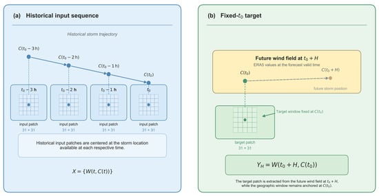
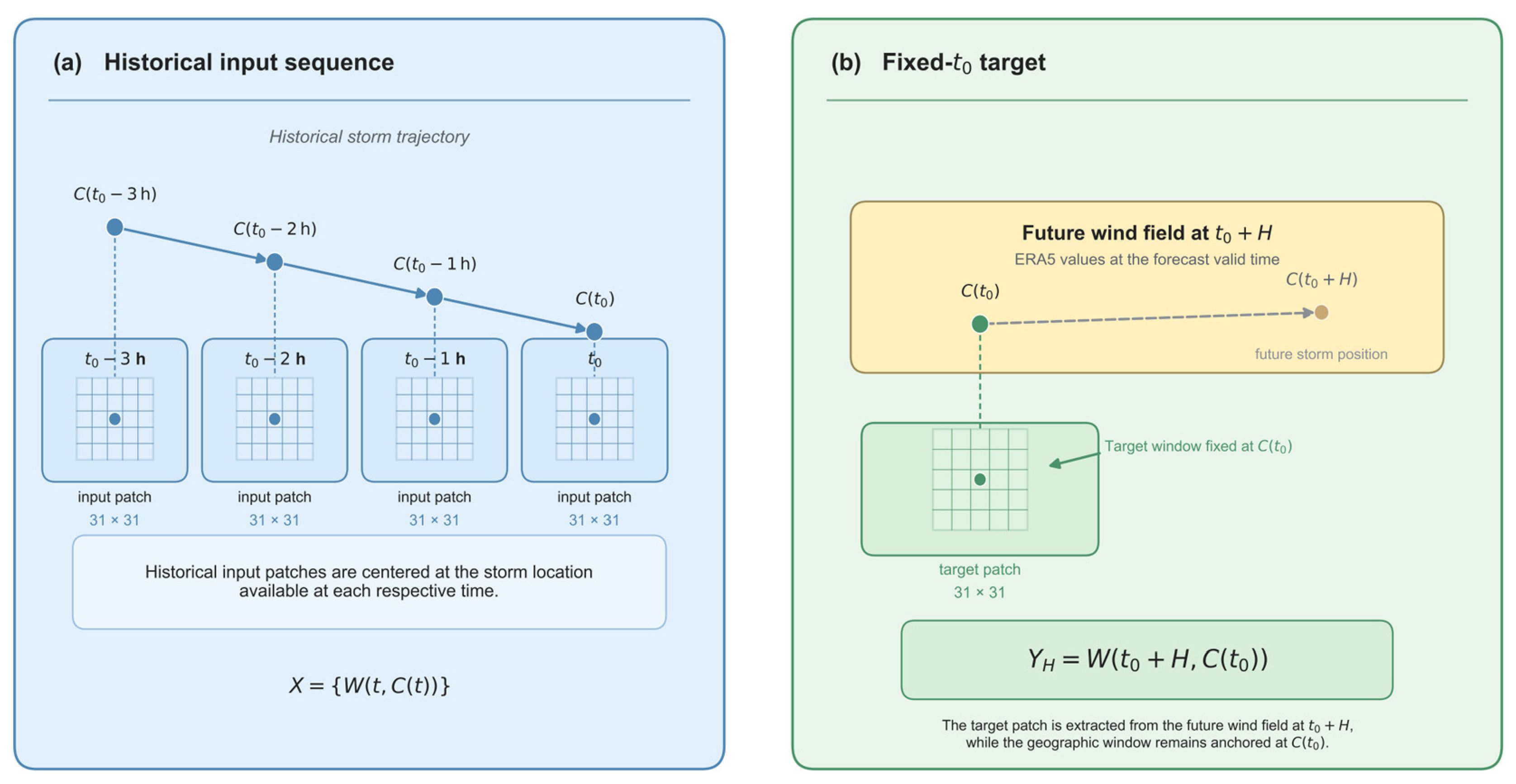
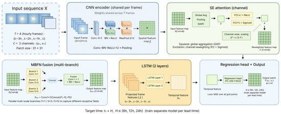
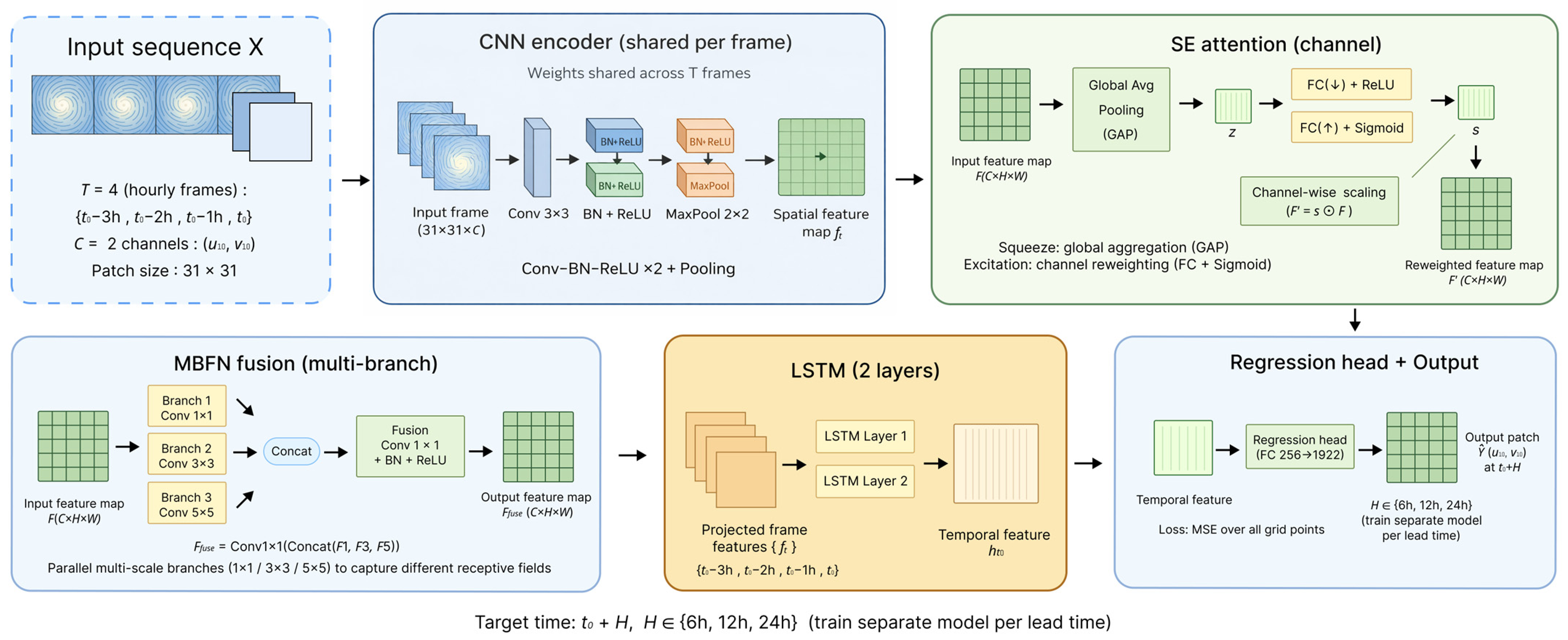
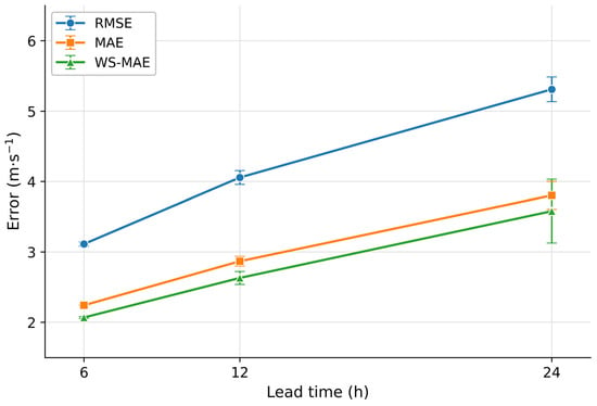
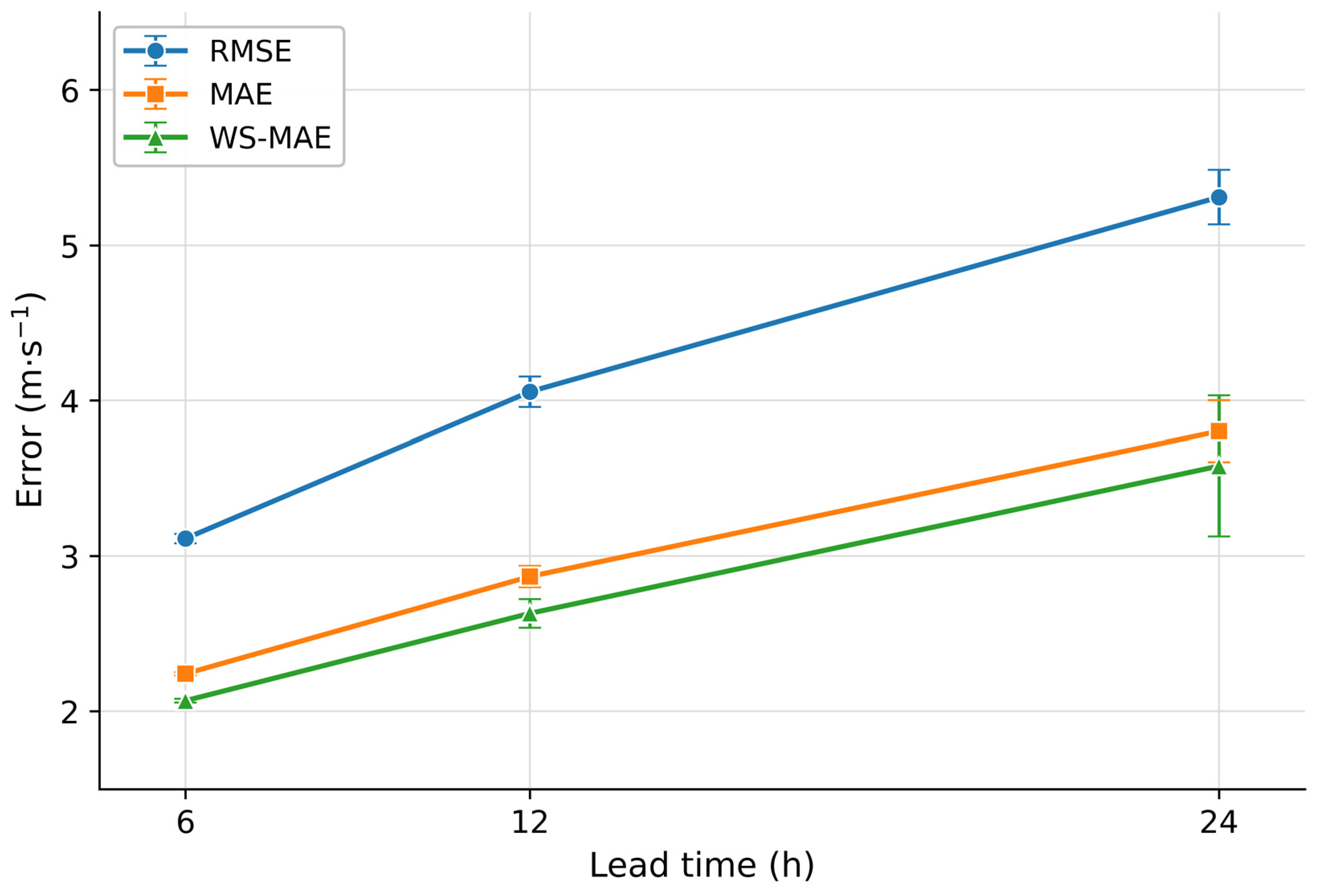
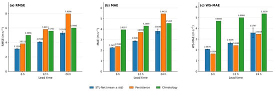
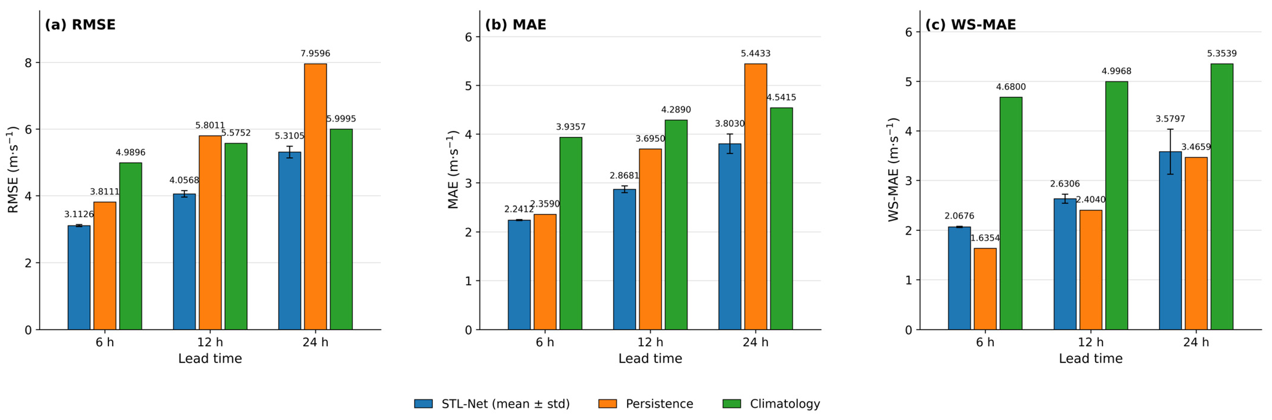
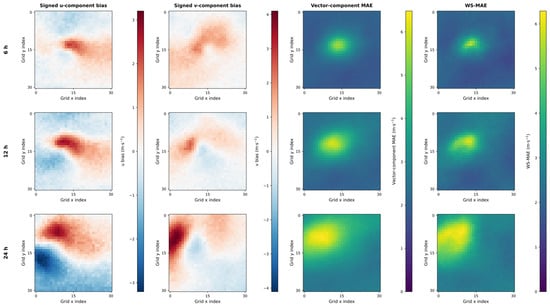
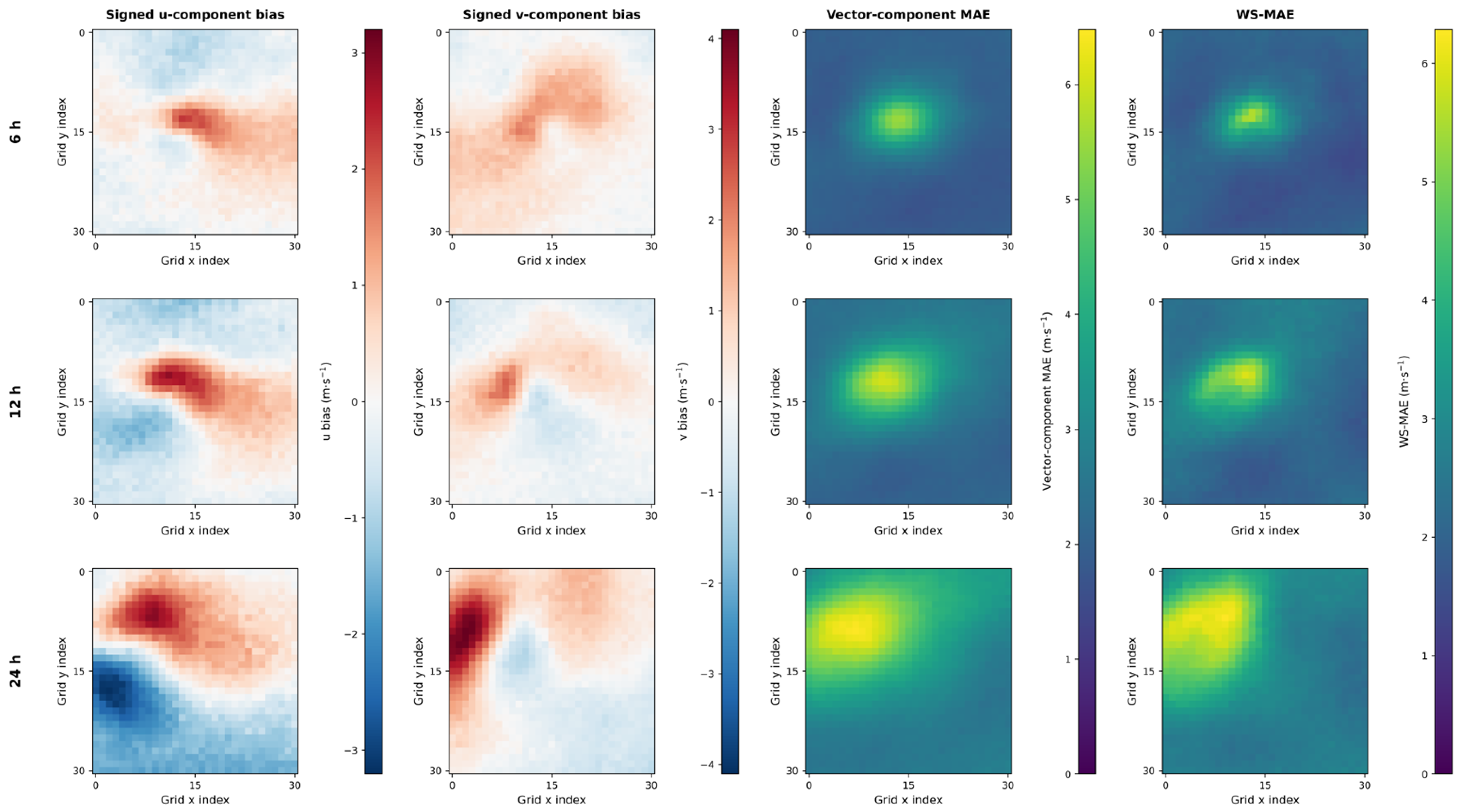

Disclaimer/Publisher’s Note: The statements, opinions and data contained in all publications are solely those of the individual author(s) and contributor(s) and not of MDPI and/or the editor(s). MDPI and/or the editor(s) disclaim responsibility for any injury to people or property resulting from any ideas, methods, instructions or products referred to in the content. |
© 2026 by the authors. Licensee MDPI, Basel, Switzerland. This article is an open access article distributed under the terms and conditions of the Creative Commons Attribution (CC BY) license.