


Abstract
Fine particulate matter (PM2.5) over the Arabian Peninsula is poorly monitored at the surface. This study emulates the relative change in summer (June–August) PM2.5 between 2020 and 2025 in the NASA GEOS-CF composition system with interpretable ensemble machine learning, using thirteen predictors from Sentinel-5P TROPOMI, ERA5-Land, CHIRPS, and MODIS Aqua on the native 0.25° grid (3933 cells), and tests how far the resulting skill transfers in space. Under 10 × 10 spatial blocking, tree-based ensembles reached cross-validated R2 = 0.82–0.84, against 0.55 for linear regression. An identically tuned Random Forest using only latitude and longitude performed better (R2 = 0.91) and remained better under larger blocks, exclusion buffers, and four of five held-out sectors; combined with the coordinates, the predictors added only modest skill. The predictor model lost all skill once training cells within 300 km were excluded, failed on an unseen eastern sector containing the single contiguous cluster of changes above +40% (r = 0.11), and did not transfer to other summers, and interpolation of the reference filled simulated gaps more accurately than every emulator. The leading predictor, the total-column O3 change, is a latitudinal gradient (r = 0.94). Split-conformal intervals under a separated spatial design covered 82–98% of test cells at the 90% nominal level but 60% in the eastern sector. The spatially blocked skill of such emulators is therefore interpolative and should be reported together with transfer diagnostics.
1. Introduction
Fine particulate matter (PM2.5), defined as particles with an aerodynamic diameter of 2.5 µm or less, constitutes a major environmental health risk worldwide and has been associated with approximately 6.7 million premature deaths annually through cardiovascular, pulmonary, and neurological disease [1]. Beyond its direct health impact, PM2.5 exerts substantial radiative forcing through aerosol–radiation and aerosol–cloud interactions, perturbs the regional hydrological cycle, and degrades visibility across densely populated arid regions [2]. Characterizing PM2.5 variability—and particularly its deviation from climatological conditions—is therefore of fundamental importance to aerosol science and public-health policy, especially where short-lived high-pollution episodes dominate the annual exposure distribution.
The Arabian Peninsula is among the most challenging environments worldwide for characterizing PM2.5 dynamics. The region combines hyper-arid desert surfaces, persistent shamal and haboob wind systems that generate episodic mineral-aerosol loading, summer solar irradiance exceeding 700 W m−2 that drives photochemical secondary-aerosol production, and extensive petrochemical activity concentrated in Kuwait, eastern Saudi Arabia, Bahrain, and Qatar [3,4]. These co-occurring processes render PM2.5 variability strongly nonlinear and spatially heterogeneous, governed by the simultaneous interaction of natural dust emission, anthropogenic combustion sources, photochemical transformation, and thermodynamic boundary-layer dynamics [5]. Resolving such variability would, in principle, require a dense and continuous surface observing system. In practice, however, ground-based air-quality networks in the region are spatially sparse, temporally discontinuous, and unevenly distributed, with little coverage of the interior deserts, southern Yemen, and rural Oman. The combination of complex, interacting forcings and limited surface observation therefore motivates the use of satellite retrievals and model-based products to characterize PM2.5 variability at the regional scale.
Satellite remote sensing and atmospheric composition modeling have accordingly become the primary means of filling these observational gaps [6]. The Copernicus Sentinel-5 Precursor TROPOMI instrument provides near-daily column densities of PM2.5 gaseous precursors and co-emitted species, including tropospheric NO2, CO, HCHO, SO2, and CH4, as well as the total (stratospheric plus tropospheric) ozone column [7]. The NASA GEOS Composition Forecast system (GEOS-CF) supplies spatially continuous, model-based PM2.5 fields generated by the GEOS-Chem chemistry module within the GEOS Earth-system framework [8]; it must be emphasized that these fields are simulated concentrations, not observations. TROPOMI columns and GEOS-CF fields have already been combined to document post-pandemic air-quality changes over the Arabian Peninsula itself [9]. MODIS Aqua land-surface temperature (LST) and vegetation-index retrievals contribute boundary-condition information on surface thermal state and bare-soil emission potential [10,11], and the diagnostic value of MODIS day/night LST records for characterizing surface thermal regimes and their trends in arid North African and Middle Eastern settings has been demonstrated in a series of regional studies [12,13,14], including machine-learning downscaling of MODIS LST in a hyper-arid megacity [15] and multi-decadal, multi-variable MODIS assessments on fixed analysis grids [16]. The ERA5-Land reanalysis provides the meteorological context within which aerosol transport, dilution, and deposition occur [17]. Synthesizing these heterogeneous, multi-resolution data streams requires statistical-learning methods capable of representing nonlinear feature interactions without restrictive parametric assumptions.
Among the methods that have emerged in aerosol research over the past decade, ensemble machine learning (ML) occupies a central place. Random Forest and gradient-boosting architectures (XGBoost, LightGBM, CatBoost) have outperformed linear regression in environmental-modeling problems characterized by nonlinear interactions, high-dimensional predictor spaces, and threshold-dependent processes, including satellite-based PM2.5 estimation [18,19] and, more recently, the modeling of surface thermal environments in arid industrial settings [20]. Their application to geospatial data, however, introduces a fundamental methodological challenge: standard random k-fold cross-validation can assign spatially correlated observations to training and validation partitions simultaneously, producing optimistic performance estimates that do not reflect true out-of-sample generalization to unobserved locations [21,22,23,24]. Despite growing awareness of this issue in the environmental-modeling literature, spatially rigorous cross-validation (CV) designs remain under-utilized in regional air-quality ML studies, particularly over the Arabian Peninsula, where the spatial heterogeneity of aerosol forcing further amplifies the risk of performance overestimation [25].
Beyond predictive performance, model interpretability is equally critical for scientific inference. Ensemble learners are often considered “black-box” methods, which limits their adoption in process-oriented atmospheric research. Shapley Additive Explanations (SHAP) address this limitation by decomposing model outputs into additive per-predictor contributions grounded in cooperative game theory [26], facilitating the identification of dominant predictive indicators, the exploration of nonlinear response patterns, and the detection of interaction effects not captured by traditional importance metrics. A complementary development is distribution-free uncertainty quantification through conformal prediction, which supplies finite-sample coverage guarantees for the outputs of any regression model [27]. It must be stressed, however, that interpretability techniques characterize associations within a fitted model; they do not, by themselves, establish physical causation.
Three design choices of the present study require explicit justification at the outset. First, the estimation target is the relative change in JJA-mean PM2.5 between the first (2020) and the last (2025) summers of the record in the GEOS-CF system, rather than surface-measured PM2.5. The study is therefore framed as statistical emulation and an assessment of spatial transfer: it asks whether a lightweight statistical surrogate driven by observable satellite and reanalysis quantities can reproduce the spatial structure of the 2020→2025 change simulated by a state-of-the-art composition model over the Arabian Peninsula, and how far that reproduction holds beyond the neighborhood of the cells used for training. All skill metrics computed against GEOS-CF are interpreted strictly in this emulation sense. An observation-anchored accuracy assessment would require reference-grade surface monitors distributed across the domain; as Section 2.11 documents, the few monitors that exist are confined to isolated urban locations and cannot support a defensible regional evaluation, so the paper is explicit—in its title, terminology, and limitations—that it certifies fidelity to the reference product, not accuracy against the true near-surface concentration field. Second, the analysis is restricted to summer (June–August, JJA) because aeolian dust activity and particulate loading over the peninsula peak in late spring and summer, when the northwesterly shamal regime is most active [28,29,30]; photochemical production of secondary aerosol is maximal under peak insolation; and extreme heat co-occurs with peak particulate exposure, making JJA the season of greatest health and policy relevance in this region—in contrast to the wintertime PM2.5 maxima typical of mid-latitude urban environments. Third, the predictors and the target are contemporaneous changes between the same two summers; the framework therefore performs estimation (reconstruction) of one change field from concurrent predictor changes rather than forecasting of future conditions, and the terminology used throughout this paper reflects that distinction.
The research gap addressed here is specific. Regional machine-learning studies of PM2.5 over the Arabian Peninsula and comparable arid regions have reported high cross-validated skill from satellite and reanalysis predictors [5,18,19,25], but none has tested whether that skill survives the validation designs now recommended for spatial prediction—block sizes commensurate with the autocorrelation range, exclusion buffers, and held-out geographic sectors [21,23,24,31,32]—or whether the predictors carry information beyond what the spatial coordinates of a cell alone would provide. Nor has the exchangeability assumption underlying conformal intervals been confronted with spatial dependence in such applications. Within this explicitly delimited scope, the study makes four contributions: (i) it develops and tunes a multi-algorithm ensemble emulator of the 2020→2025 summer PM2.5 change in GEOS-CF on the native grid of the reference, under a nested spatial block GroupKFold cross-validation (CV) design; (ii) it quantifies, for a regional aerosol emulator, how the reported skill depends on block size, exclusion-buffer distance, and held-out sectors, compares it under each of these designs with an identically tuned model that uses only the coordinates of a cell, and tests the emulator against interpolation of the reference in a simulated missing-cell experiment, thereby establishing whether the predictors carry transferable information beyond position; (iii) it identifies the dominant predictive indicators through a tri-metric importance analysis and shows that the leading predictor, the total-column O3 change, acts as a smooth latitudinal proxy rather than as a photochemical signal; and (iv) it implements split-conformal intervals under a fully separated spatial train/calibration/test design and reports their coverage as an empirical diagnostic. Together these elements provide a transparent protocol for establishing what satellite-predictor emulation of coarse composition-model fields can and cannot deliver in data-sparse arid regions. Supporting figures and the dataset inventory are provided in Appendix A and Appendix B.
2. Materials and Methods
2.1. Study Area and Seasonal Focus
The study domain encompasses the Arabian Peninsula and its surrounding margins, bounded by longitudes 32.01° E–61.38° E and latitudes 3.15° N–32.40° N (Figure 1). The region is among the most climatically extreme environments on Earth, distinguished by hyper-arid desert surfaces, persistent mineral-dust emission driven by the shamal and haboob wind systems, intense summer solar irradiance exceeding 700 W m−2, and active photochemical processing that promotes the formation of secondary aerosols and tropospheric ozone [3,4]. These characteristics render summer PM2.5 variability exceptionally complex, governed by the nonlinear interaction of primary dust emission, secondary-aerosol formation, transboundary industrial pollution transport from the petrochemical-dense northeastern subregion, and thermodynamic boundary-layer dynamics [5].
Figure 1.
Study domain and summer atmospheric drivers over the Arabian Peninsula, shown as JJA means over 2020–2025 on the native 0.25° analysis grid: (a) GEOS-CF PM2.5, with major cities (triangles), the 10 × 10 spatial-block grid used for cross-validation (thin lines), and the two subregions used in the stratified evaluation (dashed boxes); (b) TROPOMI total-column O3; (c) MODIS Aqua daytime land-surface temperature; and (d) TROPOMI CO column.
The analysis uses the six consecutive summers 2020–2025, each defined as June, July, and August (JJA). The summers 2020 and 2025 define the change field that is modeled (Section 2.3); the intermediate summers 2021–2024 are used only for the temporal-transfer test of Section 2.12. This seasonal focus reflects the regional phenology of particulate pollution rather than convention: over the Arabian Peninsula, dust-storm frequency and aerosol loading peak in late spring and summer under the “40-day” shamal regime [28,29,33], so that—unlike mid-latitude urban environments, where PM2.5 typically peaks in winter—JJA is the season of most-severe and most-variable fine-particle pollution in this domain. Summer additionally maximizes photochemical secondary-aerosol production and coincides with extreme-heat exposure, so that the health burdens of PM2.5 and heat compound each other. The reference summer, 2020, coincides with the emission anomaly associated with COVID-19 mobility restrictions and with anomalous shamal activity; the implications of this choice of reference for the interpretation of the change field are addressed in Section 2.3, Section 4.2 and Section 4.5.
2.2. Datasets
All input data were acquired and preprocessed within the Google Earth Engine (GEE; Google LLC, Mountain View, CA, USA) cloud-computing platform [34], which has become a standard environment for multi-year thermal and land-surface analyses over arid regions [16,20,35] and which provided server-side processing of the multi-year, multi-source raster archive without local data transfer. For each year of the study period, collections were filtered to the JJA months, temporally averaged across all available observations, clipped to the study domain, and exported as single-band GeoTIFF files in WGS84 geographic coordinates (EPSG:4326). CHIRPS precipitation is the one exception to the averaging rule: daily values were summed over the days of the seasonal window, so that the variable is the seasonal precipitation total rather than a mean.
The target (reference) variable is the PM2.5 mass concentration of the NASA GEOS Composition Forecast system, version 1 (GEOS-CF v1) [8], specifically the band PM25_RH35_GCC, which represents fine particulate matter at 35% relative humidity from the GEOS-Chem atmospheric-chemistry component at a native resolution of 0.25° (≈27.5 km). Throughout this paper, these values are referred to as the “GEOS-CF reference” (never as observations), and all skill statistics computed against them are emulation metrics in the sense defined in Section 1. Four independent sources provided thirteen predictor variables representing atmospheric composition, meteorological state, and land-surface conditions. Atmospheric composition was characterized using six column retrievals from the Sentinel-5P TROPOMI offline Level-3 products [7]: the tropospheric NO2 column, the total CO, HCHO and SO2 columns, the column-averaged CH4 mixing ratio, and the total ozone column. The ozone variable requires emphasis. The band used (O3_column_number_density of COPERNICUS/S5P/OFFL/L3_O3) is the total ozone column, which integrates the stratospheric and tropospheric burden; over this domain it averages 0.127 mol m−2 (≈286 Dobson units; Figure 1b), of which roughly 90% resides in the stratosphere [36]. It is therefore a measure of the total ozone burden and not of near-surface photochemistry; the consequences for the interpretation of the results are developed in Section 3.6 and Section 4.1. The TROPOMI products have a native sensor footprint of ≈5.5 km × 3.5 km, are distributed as 0.01° Level-3 grids, and were aggregated to the analysis grid described in Section 2.4. Meteorological forcing was represented by five variables: 2 m air temperature, surface pressure, 10 m wind-speed magnitude computed as the Euclidean norm of the zonal and meridional components (WS = √(u2 + v2)), and relative humidity approximated from air and dew-point temperature via the Magnus formula, all from the ERA5-Land daily-aggregated reanalysis (≈9 km) [17], together with the seasonal total precipitation from the CHIRPS daily product (≈5.6 km) [37], selected for its superior performance over arid environments relative to reanalysis precipitation fields [38]. Land-surface conditions were represented by MODIS Aqua daytime and nighttime LST (MYD11A1, Collection 6.1, 1 km) [10], converted to °C using the product scale factor (DN × 0.02 − 273.15), and NDVI (MYD13Q1, Collection 6.1, 250 m) [11], rescaled to dimensionless units (DN × 0.0001). The full variable inventory, including native resolutions and the transformation applied to each variable, is presented in Table A1 (Appendix A).
Satellite aerosol optical depth (AOD), the predictor most widely used in PM2.5 estimation studies [39], was deliberately not included, for three reasons. First, AOD retrieval over the bright, hyper-arid surfaces that dominate this domain is comparatively uncertain: it depends on specialized algorithms such as Deep Blue, retains residual surface-reflectance artifacts, and loses coverage during precisely the heavy-dust and cloud-contaminated conditions of greatest interest here [40]. Second, AOD is a column-integrated quantity whose relationship to near-surface PM2.5 is confounded by the elevated dust layers that are frequent over the peninsula in summer, so that the column-to-surface conversion introduces its own model dependence. Third, and specific to the emulation design of this study, excluding AOD provides a stringent test of whether gaseous-precursor, meteorological, and land-surface information alone suffices to reconstruct the reference-change field, and it avoids near-circularity with aerosol-based data in prospective extensions of the framework to observation-anchored targets. The incorporation of MAIAC AOD is nevertheless identified as a priority extension in Section 5.
2.3. Definition of the Change Fields and Preprocessing
The quantity modeled in this study is the change in the JJA mean of each variable between the first and the last summers of the record, 2020 and 2025. For a native-grid cell p and a ratio-scale variable X—one whose zero is physically meaningful and whose 2020 value is bounded away from zero—the change is expressed as a percentage of the 2020 reference value,
whereas for interval-scale variables, and for ratio-scale variables whose 2020 reference values approach zero, the absolute change
is used instead. Equation (1) applies to the GEOS-CF PM2.5 target and to the NO2, CO, HCHO, total-column O3, CH4, surface-pressure, relative-humidity, and rainfall predictors, whose 2020 reference values are strictly positive at every cell and whose first-percentile reference value exceeds 30% of the domain median (Table A1); the CHIRPS seasonal totals, in particular, have a minimum of 10 mm and a median of 90 mm, so that the denominator of Equation (1) is never small for rainfall. Equation (2) applies to the three temperature variables (2 m air temperature, daytime and nighttime LST; change in kelvin), because a percentage change in Celsius temperature depends on the arbitrary zero of the scale and has no physical meaning; to NDVI (dimensionless change), whose 2020 values are ≤0 at three cells and below 0.05 over bare desert, where Equation (1) yields changes of thousands of percent; and to wind speed (m s−1), whose 2020 seasonal means fall to 0.04 m s−1 and whose first-percentile value is only 10% of the median, so that Equation (1) produces a heavy-tailed, denominator-dominated distribution. The target field is therefore the relative change in JJA-mean PM2.5 between the pandemic-perturbed summer of 2020 and the most recent summer of the record, and every performance statistic in this paper refers to the spatial reconstruction of this single field (n = 3933 native cells; Section 2.4) from the contemporaneous predictor changes. The pair (2020, 2025) was selected because it spans the full record and therefore carries the largest interannual contrast available; the choice of 2020 as the reference—a summer of depressed anthropogenic emissions and elevated dust loading—is a limitation that is examined in Section 4.2 and Section 4.5, and the transferability of the fitted relationships to the other change fields of the record is tested explicitly in Section 2.12.
D(p) = X(p,2025) − X(p,2020),
No native cell lacked a target value. Missing predictor values—arising from cloud masking in optical retrievals and from TROPOMI coverage gaps, and affecting 38.5% of cells for CH4, 1.7% for wind speed, and ≤0.5% of cells for each of the remaining predictors—were imputed within the ML pipeline using the column-wise median, a strategy robust to the skewed distributions of the change fields. The large gap fraction of CH4 limits any inference about its role and is listed among the limitations (Section 4.5). All predictors were subsequently standardized to zero mean and unit variance (z-score transformation) to ensure equitable contribution across variables with disparate physical units. Imputation and scaling parameters were fitted exclusively on the training partitions within each CV fold to prevent information leakage from held-out observations.
SO2 was excluded from the final predictor set on signal-to-noise grounds. TROPOMI SO2 columns over the predominantly low-SO2 background of the study domain lie close to the retrieval detection limit, where the differential optical absorption spectroscopy fit yields noise-dominated column values that are frequently negative [41]: the 2020 reference value is ≤0 at 50 of the 3933 native cells and its median (9.8 × 10⁻⁵ mol m−2) is of the order of the retrieval noise. The denominator of Equation (1) is therefore vanishingly small or negative for this species, and the percentage-change transformation is numerically unstable, producing physically uninterpretable magnitudes and signs (first and 99th percentiles of −256% and +51%); an absolute change would be dominated by retrieval noise. SO2 was therefore removed prior to model fitting.
2.4. Analysis Grid and Effective Spatial Resolution
The predictors and the reference were brought onto a common grid in two steps. First, every annual JJA layer was exported from GEE as a raster on a 0.01° (≈1 km) grid; the GEOS-CF reference and the coarser predictors were assigned to this grid by nearest-neighbor resampling, the GEE default, and the finer MODIS products (1 km and 250 m) were exported on the same grid. Second, values were extracted at the 4849 points of a regular sampling grid with a spacing of 0.2246° (25 km), each point taking the value of the 1 km export at its location. Because this spacing is finer than the 0.25° native grid of the GEOS-CF reference, the sample points do not map one-to-one onto native cells: they fall within 3933 distinct native cells (3113 cells sampled once, 771 twice, two three times, and 47 four times), and points within one native cell carry identical reference values, confirming that the reference was not interpolated. All points were then assigned to their native cell (cell index = ⌊(coordinate + 0.125°)/0.25°⌋ in each direction); the reference value was taken once per cell; and the predictor value of each cell was computed as the mean of the yearly values at the one to four points falling within it, before the changes in Equations (1) and (2) were formed. The predictors are therefore point samples at 1 km support, averaged over at most four locations per cell, and not area means over all 1 km pixels of the ≈27 km cell. The resulting dataset contains exactly one record per native cell (n = 3933), with cell centers at multiples of 0.25°, and the number of distinct reference values equals the number of records.
Because the predictors are point samples rather than area means, the dependence of the results on sampling support was examined directly (Table A5). Sub-cell variability was first estimated from the semivariance of each predictor change between neighboring sample points 25 km apart, expressed as a fraction of its total variance: the fraction is at most 0.06 for the total-column O3, air-temperature, wind-speed, relative-humidity, and rainfall changes, 0.21–0.25 for the two LST changes, 0.36–0.43 for the NO2, CO, CH4, and NDVI changes, and 0.62 and 0.91 for the surface-pressure and HCHO changes, against 0.005 for the reference. For the last two groups, a single 1 km sample is a noisy estimate of the cell mean. The analysis was then repeated with three alternative aggregations. Replacing the cell mean by one randomly selected point (five draws) or by the point nearest the cell center changed the fold-mean CV R2 of the Random Forest from 0.815 to 0.806–0.808 and the CV RMSE from 7.11% to 7.24–7.29%, and left the permutation-importance ranks of the O3, daytime-LST, and CO changes unchanged (1, 2, and 4). Averaging the points over a 3 × 3 neighborhood of native cells (≈75 km support, larger than a cell) raised the CV R2 to 0.886 and moved the CO change to first rank, ahead of the O3 and daytime-LST changes. A true area mean over each ≈27 km cell has a support between these bounds; its exact effect could be established only by re-exporting the predictors from GEE with an area-mean reducer onto the native GEOS-CF grid, which was not done. The bounds nevertheless show that the choice between one and four point samples per cell is immaterial, that the absolute skill and the order of the leading predictors depend on the sampling support, and that the central findings of Section 3.6—the predictors do not outperform the cell coordinates and do not transfer to distant regions—hold under the smoothest support tested.
Two further properties of this design bear on inference. First, the analysis is conducted at the native 0.25° resolution of the coarsest input; no sub-native information is claimed—that would require a dedicated downscaling design with independent fine-scale validation [15]—and intra-urban applications lie outside the scope of the framework. Second, the dataset contains no replicated records of the same reference cell, so that the sample size equals the number of distinct spatial units. Spatial dependence between distinct neighboring cells nevertheless remains very strong (Moran’s I of the target field = 0.99), and its consequences for validation are examined through the blocked, buffered, and sector-based designs of Section 2.5 and Section 2.12 [21,23].
2.5. Spatial-Block Cross-Validation
A fundamental challenge in geospatial ML is the positive spatial autocorrelation of environmental observations, which causes standard random k-fold CV to assign spatially proximate—and therefore statistically dependent—observations to training and validation folds simultaneously. This spatial data leakage produces optimistic performance estimates that do not reflect true out-of-sample generalization; Schratz et al. [22] demonstrated that non-spatial CV overestimates predictive accuracy by 24–30% relative to spatially blocked designs in analogous environmental-modeling tasks, and Ploton et al. [23] documented comparable inflation in large-scale ecological mapping.
To address this, the native-grid dataset was partitioned into a regular 10 × 10 grid over its extent (longitude 34.75–59.75° E; latitude 12.75–32.0° N), yielding 68 non-empty spatial blocks of 2.5° × 1.93° (≈255 km × 214 km). Each cell was assigned an integer block identifier derived from its longitudinal and latitudinal bin indices (block_id = lon_bin × 10 + lat_bin), and cells sharing an identifier were assigned to the same CV group, so that no two cells from the same block are split between training and validation partitions. This configuration is the reference design of the study; its adequacy is examined below and tested directly in Section 2.12.
The spatial-dependence structure of the target field was characterized by its empirical semivariogram (Figure A9). Semivariance rises monotonically across all resolvable lags—attaining about 22% of the field variance at the block dimension (≈250 km), one half near ≈575 km, and the full variance only near ≈975 km, without a clear sill within the domain—the signature of basin-scale organization dominated by the east–west dipole of the change field (Section 3.3). Blocks of the order of this dependence range are infeasible within a domain of ≈2400 km × 2100 km, and blocked CV with 10 × 10 blocks therefore removes short-range but not long-range dependence between training and validation cells: neighboring blocks enter training and validation simultaneously. For this reason the outer-CV estimate is not described here as unbiased, nor its folds as independent. Instead, the dependence of the skill on the validation design is quantified explicitly—by varying the block size from 3 × 3 to 20 × 20, by excluding training cells within 100–400 km of the validation block, and by holding out entire geographic sectors (Section 2.12)—following the recommendations of Roberts et al. [21], Ploton et al. [23], and Meyer and Pebesma [24,31], and acknowledging the continuing debate on what spatial cross-validation estimates [32].
Group-based CV was implemented using a nested design: an outer loop of 10-fold GroupKFold on the 68 blocks for performance estimation, and an inner loop of 5-fold GroupKFold, likewise on blocks, for hyperparameter tuning and for the generation of stacking meta-features (Section 2.6). To ensure compatibility with the scikit-learn GridSearchCV interface across versions, fold indices were pre-computed as explicit (train_index, val_index) pairs and passed directly as the cv argument rather than relying on implicit group routing via fit parameters. This nested spatial-CV design follows the recommendations of Roberts et al. [21] for data with hierarchical or spatial dependency structures.
2.6. Machine-Learning Models and Hyperparameter Optimization
Six regression models spanning a linear parametric baseline and five nonlinear ensembles were evaluated. Because all are established methods, only brief characterizations are given here, and readers are referred to the original algorithmic publications. Multiple linear regression (MLR) served as the parametric baseline against which the gain attributable to nonlinear modeling is quantified. Random Forest (RF) is a bagging ensemble of decorrelated regression trees [42]. XGBoost is a regularized gradient-boosting system employing a second-order approximation of the loss [43]. LightGBM accelerates gradient boosting through gradient-based one-side sampling and exclusive feature bundling [44]. CatBoost implements ordered boosting with permutation-driven target statistics to eliminate prediction shift [45]. The stacking ensemble combines the four tuned tree-based learners as level-0 models with a ridge-regression meta-learner (α = 1) trained on their out-of-fold predictions; ridge regularization prevents the meta-learner from overfitting to the highly correlated predictions of architecturally similar base models. The out-of-fold meta-features are generated with a spatially grouped 5-fold GroupKFold on the training blocks of each outer fold; a variant using a shuffled, non-spatial KFold is compared in Section 3.1. Out-of-sample estimates for performance evaluation are generated strictly within the outer 10-fold spatial GroupKFold loop, so that no cell used in outer evaluation is seen during training at any stage of the pipeline.
Hyperparameters of all four tree-based models were tuned by exhaustive grid search (GridSearchCV) on the pre-computed inner 5-fold spatial GroupKFold splits, with CV R2 as the scoring criterion; uniform tuning across models ensures that performance differences reflect architectural rather than tuning-effort effects. The complete search spaces and the selected configurations are consolidated in Table 1, and all selected combinations were archived in a dedicated output file (00_Best_Hyperparameters.csv) for reproducibility. All analyses were performed in Python 3.13 with scikit-learn 1.9.1, XGBoost 3.4.1, LightGBM 4.7.0, CatBoost 1.2.10, SHAP 0.53.0, libpysal 4.15.0, esda 2.10.0, SciPy 1.18.1, and Matplotlib 3.11.2.
Table 1.
Hyperparameter search spaces and selected configurations for the four tree-based models (native-grid analysis). All models were tuned by exhaustive grid search on the inner 5-fold spatial GroupKFold with CV R2 as the criterion; p denotes the number of predictors.
2.7. Model Evaluation Metrics and Stratified Evaluation
Model performance was quantified using four complementary metrics computed exclusively on out-of-sample cross-validated estimates. The coefficient of determination (R2) measures the proportion of variance in the reference 2020→2025 change in PM2.5 explained by the model relative to a mean-prediction baseline. Root mean square error (RMSE, %) penalizes large errors quadratically and is therefore sensitive to the high-magnitude changes of primary interest here. Mean absolute error (MAE, %) provides a linearly weighted, interpretable average error magnitude less sensitive to extreme outliers. The Nash–Sutcliffe efficiency (NSE) is defined as
where NSE = 1 denotes a perfect model, NSE = 0 indicates performance equivalent to the reference mean, and NSE < 0 indicates that the mean outperforms the model [46,47]. All metrics are reported as cross-validated means and standard deviations across the 10 outer spatial folds, and the train–CV R2 gap (ΔR2) is reported as a direct diagnostic of overfitting magnitude.
Because the motivation of this study emphasizes episodic high-pollution conditions, aggregate metrics are complemented by stratified reporting. Out-of-sample performance is computed separately (i) for terciles of the reference-change distribution (tercile boundaries at −3.1% and +17.9%); (ii) for extreme cells, defined as cells whose reference change exceeds +40%, whose spatial contiguity is examined in Section 2.12; and (iii) for three physiographically distinct subregions delineated from the coherent residual clusters of Figure A3—the northeastern industrial corridor (46.0–53.5° E, north of 23.5° N; Kuwait, eastern Saudi Arabia, Bahrain, Qatar, and the western UAE), the southeastern (Omani) coastal sector (east of 52° E, south of 24° N), and the remaining interior and west. Because the target is a seasonal-mean change, the extreme stratum describes cells with an extreme seasonal-mean change, not short-lived pollution episodes, which a seasonal mean cannot resolve. Within-stratum R2 deserves a caution stated in advance: it is computed against the stratum’s own mean, so that a stratum with deliberately restricted variance can return a low or negative R2 even when the pooled model is skillful; RMSE, MAE, and mean bias are therefore the primary stratum-level metrics, and R2 is reported for completeness. The stratified results appear in Section 3.2 and prevent the aggregate R2 from concealing regime-dependent weaknesses.
2.8. Feature-Importance Analysis
To reduce the risk of misleading rankings from any single metric, three methodologically complementary importance measures were computed for the tuned RF model. The mean decrease in impurity (MDI) quantifies the average reduction in node variance attributable to splits on each feature, summed across nodes and averaged across all 300 trees; MDI is computationally efficient but upwardly biased for continuous and high-cardinality predictors [48] and was therefore interpreted in conjunction with the two metrics below. Permutation importance measures the mean decrease in CV R2 when each feature’s values are randomly permuted, averaged over 30 repetitions to stabilize the estimate [42]. SHAP values decompose each individual model output into additive feature contributions satisfying the efficiency, symmetry, dummy, and linearity axioms [26], and were computed with the TreeExplainer algorithm, which exploits the recursive tree structure for exact polynomial-time computation. Mean absolute SHAP values were used as the global importance metric; beeswarm plots visualize the direction and distribution of contributions, and dependence plots characterize the functional form of the marginal effects of the three top-ranked features. A consensus ranking was derived by averaging the ordinal ranks assigned by MDI, permutation importance, and mean |SHAP| across all thirteen predictors. It is emphasized that all three metrics characterize predictive associations within the fitted emulator; the language used to report them (Section 3.5 and Section 4.1) is correspondingly associational, not causal.
2.9. Residual Diagnostics and Spatial-Autocorrelation Testing
Post hoc residual analysis was performed on the out-of-sample cross-validated residuals of the RF model to assess normality, homoscedasticity, and spatial independence of errors. Normality was assessed with the Shapiro–Wilk test applied to all n = 3933 cross-validated residuals; the statistic W and its p-value are reported alongside a residual histogram with the fitted normal density and a normal Q–Q plot. Heteroscedasticity was evaluated using a scale–location plot of √|standardized residuals| against fitted values with a Savitzky–Golay smoothed trend, referenced to the expectation of √|Z| for a standard-normal variable Z, 21/4 Γ(3/4)/√π ≈ 0.822. Spatial autocorrelation in cross-validated residuals was quantified with Moran’s I, computed on a k-nearest-neighbor spatial-weights matrix (k = 5) constructed from cell-center coordinates using libpysal [49]; the associated p-value tests the null hypothesis of no spatial autocorrelation under normality of the reference distribution, and the same statistic was computed for the target field itself. The spatial distribution of residuals was mapped to identify geographically coherent error zones and to inform the subregional stratification of Section 2.7.
2.10. Prediction-Interval Construction
Predictive uncertainty was quantified with split-conformal prediction intervals [27,50], using a design that separates training, calibration, and test cells by spatial block, so that no test cell contributes to the model that produces a calibration residual: of the ten outer folds, six are used to train a single Random Forest, two to calibrate, and two to test. Calibration residuals ri = yi − ŷi from the calibration folds define the interval
where q0.05 and q0.95 are the 5th and 95th percentiles of the calibration residuals. Coverage is evaluated on the test folds only. Because a single assignment of folds to roles gives one realization, the procedure was repeated over five rotations of the fold assignment and, to probe the regime of greatest interest, once more with the entire eastern sector (longitude ≥ 52° E, which contains all extreme cells) as the test region and a random fifth of the remaining blocks as the calibration set. The finite-sample coverage guarantee of split-conformal prediction requires exchangeability of calibration and test observations [27,50]; under the spatial dependence documented in Section 2.5, cells in different blocks are not exchangeable, and no guarantee is claimed. The coverage values reported in Section 3.5 are therefore empirical diagnostics of interval calibration rather than certified probabilities, in line with recent treatments of conformal inference beyond exchangeability [51]. Coverage is additionally reported by tercile of the reference change and for the extreme stratum.
2.11. Scope of Validation and the Absence of Ground-Based Evaluation
No evaluation against surface PM2.5 measurements is reported in this study, and the reasons deserve explicit statement rather than silence, because the absence of such an evaluation defines what the results can and cannot claim. Reference-grade PM2.5 monitors with publicly accessible records are confined to a handful of urban locations within a modeled domain of roughly three million square kilometers; the interior deserts, most of Yemen, and rural Oman—precisely the regions where the largest changes occur (Section 3.3)—are unmonitored. Three considerations make a station-based evaluation not merely weak but potentially misleading under these conditions. First, representativeness: an urban point monitor samples local traffic and industrial influences at the street-to-neighborhood scale, whereas each native cell represents an area average over roughly 27 × 27 km; over the strong intra-urban gradients of Gulf cities, the two quantities differ systematically even when both are correct. Second, the change formulation of Equations (1) and (2) requires a complete JJA record at a fixed instrument and location in both 2020 and 2025; discontinuous records—the norm among the accessible monitors in this region and period—break the definition itself rather than merely thinning the sample. Third, the handful of collocatable cells that would survive these constraints could not support statistically meaningful conclusions about a domain of 3933 cells, and reporting metrics from so small and geographically biased a sample would confer a false impression of observational anchoring. Satellite-based assessments in other data-sparse arid settings face the same constraint and, where in situ measurements are lacking, report their products explicitly as satellite-derived estimates rather than validated measurements [52]; the same convention is followed here. The validation of this study is therefore strictly internal—spatially blocked cross-validation against the GEOS-CF reference, together with the transfer diagnostics of Section 2.12—and every claim in this paper is bounded accordingly: the framework is demonstrated as an emulator of the reference product, its accuracy against the true near-surface concentration field is not established, and this is recorded as the first limitation in Section 4.5. Establishing observation-anchored evaluation as regional monitoring densifies is identified in Section 5 as a priority for future work. The complete workflow of the study is summarized in Figure 2.
Figure 2.
Workflow of the study: data acquisition, construction of the native-grid change fields (Equations (1) and (2)), spatial blocking and nested cross-validation, model fitting and evaluation, spatial-transfer diagnostics, interpretability and residual diagnostics, and split-conformal intervals under a three-way spatial split.
2.12. Spatial-Transfer, Ablation, Temporal-Transfer, and Missing-Cell Diagnostics
Because the semivariogram (Section 2.5) shows that no feasible block size isolates the validation cells from spatially dependent training cells, the reported skill was examined as a function of the validation design rather than reported for one design only. Four diagnostics were computed with the tuned Random Forest—the model used for all interpretability analyses—each under 10-fold GroupKFold unless stated otherwise. (i) Block-size sensitivity: The partition was varied from 3 × 3 (≈850 × 710 km; nine blocks, leave-one-block-out) through 4 × 4, 5 × 5, 7 × 7, 10 × 10, and 15 × 15 to 20 × 20 (≈130 × 110 km). (ii) Buffered cross-validation: With the 10 × 10 partition, training cells lying within 100, 200, 300, or 400 km of any validation cell were excluded from the training set of that fold [24]; the fraction of training data retained is reported alongside the skill. (iii) Held-out geographic sectors: The model was trained on all cells outside a sector and evaluated on the sector, for the eastern sector (longitude ≥ 52° E), the northeastern industrial corridor (Section 2.7), and the northern (latitude ≥ 27° N), southern (latitude < 18° N), and western (longitude < 42° E) sectors; because within-sector R2 is computed against the sector mean, the correlation coefficient r, RMSE, and mean bias are reported together with the RMSE of a baseline that assigns the training-set mean to every test cell. (iv) Coordinate and ablation baselines: The full predictor set was compared with the set without total-column O3, without O3 and daytime LST, with latitude and longitude added, with O3 replaced by latitude and longitude, with latitude and longitude alone, and with O3 alone. A model using coordinates alone is a pure spatial interpolator with no physical predictors; comparison with it reveals how much of the predictors’ skill exceeds interpolation.
Two further diagnostics address the temporal scope and the extreme cells. Temporal transfer: The Random Forest fitted to the entire 2020→2025 field was applied, without refitting, to the 2020→2021, 2020→2022, 2020→2023, and 2020→2024 change fields constructed with Equations (1) and (2) from the same inputs, and a model fitted to the 2020→2024 field was applied to the 2020→2025 field. These tests are out-of-time but not out-of-space; they establish whether the relationships learned from one change field carry over to another. Extreme cells: The cells with reference change above +40% were grouped into spatially connected clusters (8-connectivity on the native grid) to establish how many distinct spatial features they represent, and their distribution across the outer folds was recorded.
Two final diagnostics test whether the predictors carry information beyond the position of a cell under transfer conditions, and whether the emulator has practical value for filling missing cells. Matched predictor-set comparison: Random Forests with the thirteen predictors, with latitude and longitude only, and with both were tuned separately by the same grid search (max_depth ∈ {6, 10, 15}, min_samples_leaf ∈ {5, 10, 20}, max_features ∈ {√p, 0.5p, p}, 300 trees) on the inner 5-fold spatial GroupKFold of the reference blocking, and evaluated under the 10 × 10, 7 × 7, and 5 × 5 partitions, under 100 km and 200 km buffers, and on the five held-out sectors; the selected configurations were max_depth = 15 and min_samples_leaf = 5 for all three sets, with max_features = 0.5p for the two predictor sets and √p for the coordinates. Simulated missing cells: circular gaps of radius 0 (isolated cells), 50, 100, and 200 km were placed at random until at least 10% of the cells had been removed; the three Random Forests were trained on the remaining cells and compared, on the removed cells, with inverse-distance weighting (power 2, twelve nearest cells) of the reference field itself, the simplest gap-filling alternative. Ten replicates were drawn for each radius.
3. Results
3.1. Model Performance and Estimation Accuracy
Table 2 summarizes the cross-validated performance of all six models under the reference 10 × 10 blocking, and Figure 3 illustrates the corresponding metrics. The MLR baseline yielded the weakest performance (CV R2 = 0.55 ± 0.17; RMSE = 11.05 ± 2.61%; MAE = 8.89 ± 2.20%). All tree-based ensembles outperformed MLR and converged within a narrow band (CV R2 = 0.82–0.84; RMSE = 6.54–7.11%). The stacking ensemble attained the best cross-validated performance (R2 = 0.84 ± 0.07; RMSE = 6.54 ± 1.94%; MAE = 4.95 ± 1.31%), followed by CatBoost and XGBoost (R2 = 0.83), LightGBM (0.82), and RF (0.82 ± 0.08). Generating the stacking meta-features with spatially grouped rather than shuffled inner folds (Section 2.6) changed the outer-CV skill negligibly (R2 = 0.841 versus 0.840; RMSE = 6.54 versus 6.57%). Training R2 values of 0.96–0.99 give train-to-CV gaps (ΔR2) of 0.14–0.17 for the ensembles and 0.07 for MLR. These statistics quantify the fidelity of the emulation of the 2020→2025 GEOS-CF change field under one particular spatially blocked design; Section 3.6 shows how strongly they depend on that design, and they are not measures of accuracy against surface observations (Section 2.11).
Table 2.
Cross-validated performance of six models of the 2020→2025 relative change in summer PM2.5 (GEOS-CF reference) over the Arabian Peninsula on the native 0.25° grid (n = 3933), under 10 × 10 spatial blocking. Values are means ± one standard deviation across the 10 outer GroupKFold folds; ΔR2 = Train R2 − CV R2. Training NSE equals Train R2 by construction (Equation (3)) and is therefore not tabulated separately.
Figure 3.
Cross-validated performance metrics for six models of the 2020→2025 relative change in summer PM2.5 (%) over the Arabian Peninsula (10 × 10 spatial blocks). Horizontal bars represent mean values across 10 spatial GroupKFold folds; error bars denote ±1 standard deviation. Metrics are (a) CV R2, (b) CV RMSE (%), and (c) CV MAE (%).
The reference-versus-estimated scatter plots (Figure 4) reveal marked differences in behavior across architectures. MLR exhibits a systematic bias pattern: it underestimates large positive changes and overestimates values in the negative tail, with the ordinary least-squares fit diverging from the 1:1 line at both extremes—behavior consistent with a linear model’s inability to capture the nonlinear amplification of PM2.5 loading under strong dust or pollution-transport conditions. The stacking ensemble and all four tree-based models exhibit much tighter scatter around the 1:1 line throughout the central distribution (approximately −20% to +40%). Nevertheless, a consistent deviation from the 1:1 line is apparent at reference values exceeding approximately +40% across all ensemble architectures, indicating a shared tendency to underestimate the largest changes; this tendency is quantified in Section 3.2.
Figure 4.
GEOS-CF reference versus cross-validated estimated 2020→2025 relative change in summer PM2.5 (%) for six models over the Arabian Peninsula. Each panel shows out-of-sample estimates from 10-fold spatial GroupKFold cross-validation. The dashed black line denotes the 1:1 reference; the solid colored line is the ordinary least-squares fit. Model-specific CV R2 and RMSE are annotated in each panel. The horizontal axis represents the GEOS-CF modeled reference, not surface observations.
Fold-level performance distributions (Figure A1) corroborate the aggregate metrics and illuminate model stability across spatially heterogeneous subregions. MLR exhibits the largest interquartile ranges for all three metrics, with fold-level R2 ranging from 0.26 to 0.75, whereas the ensembles range from 0.60 to 0.91, with the stacking ensemble achieving the narrowest spread in RMSE and MAE. Learning-curve analysis for RF (Figure A2), computed with 5-fold spatial GroupKFold, shows a validation R2 that is negative below ≈1600 training cells, rises steeply between ≈1900 and 2500 cells as spatial coverage accrues, and reaches 0.80 at the maximum training size, while training R2 stabilizes near 0.96; the persistent gap of ≈0.16 is consistent with the ΔR2 values of Table 2.
3.2. Stratified Performance and the High-Change Cluster
Table 3 reports out-of-sample RF performance stratified by magnitude and subregion, as specified in Section 2.7. Absolute error grows with the magnitude of the change—RMSE rises from 6.61% in the lower tercile to 9.34% in the upper—and the mean bias reverses sign, from +3.75% (overestimation) in the lower tercile to −4.99% (underestimation) in the upper. The extreme stratum exposes the principal weakness: over the 51 cells whose reference change exceeds +40%, the mean bias is −28.6% and the RMSE 30.3%, so that the emulator recovers, on average, less than half of the amplitude—exactly the deviation visible in Figure 4. These 51 cells are not independent events: they form a single 8-connected cluster on the Arabian Sea coast of Oman (57.75–59.75° E, 20.0–22.25° N) that contains the domain maximum (+67.7% at 58.75° E, 21.25° N), and 49 of them fall in one outer fold. The stratum therefore characterizes one contiguous spatial feature of the seasonal-mean change field, and—because a seasonal mean integrates over the whole summer—it says nothing about the estimation of short-lived dust or pollution episodes, which the present design cannot address. Subregionally, error concentrates where the residual map (Figure A3) indicates: RMSE over the southeastern (Omani) coastal sector is 9.69% with a mean bias of −3.54%, and over the northeastern industrial corridor 8.69% with a bias of −4.25%, against 6.53% and +1.42% over the interior and west, where within-stratum R2 remains high (0.79). The stacking ensemble reproduces the pattern with marginally smaller errors (extreme-cluster bias −25.1%; Omani-sector RMSE 9.03%), confirming that the weaknesses are shared across architectures. The aggregate CV R2 of 0.82–0.84 is thus dominated by the well-estimated central part of the distribution and must not be read as uniform skill across magnitudes or subregions.
Table 3.
Out-of-sample Random Forest performance stratified by reference-change magnitude and by subregion (definitions in Section 2.7; native grid, n = 3933). The extreme stratum comprises the 51 cells with reference change above +40%, which form one contiguous cluster on the Omani coast (Section 3.2); mean bias is estimated minus reference, so negative values denote underestimation. Within-stratum R2 is computed against the stratum mean and can be negative under restricted within-stratum variance even when pooled skill is high (pooled out-of-fold R2 = 0.82); RMSE, MAE, and bias are the primary stratum-level metrics.
3.3. Spatial Distribution of the 2020→2025 PM2.5 Change
Figure 5 maps the 2020→2025 relative change in summer PM2.5 of the GEOS-CF reference, and Figure 6 compares it with the cross-validated ML estimate and their difference. The field is organized as a pronounced east–west dipole. A broad belt of positive change occupies the eastern half of the peninsula, intensifying toward the southeastern (Omani) coastal sector, where the field attains its maximum of +67.7% at 58.75° E, 21.25° N on the Arabian Sea coast; elevated positive values also extend along the Arabian Gulf littoral from Kuwait to the UAE. Negative change dominates the north-central and northwestern interior of Saudi Arabia, reaching a minimum of −23.3% at 44.25° E, 26.25° N. The domain-mean change is +7.2%, with 62.6% of cells positive, reflecting a rise in the domain-mean JJA PM2.5 of the reference from 32.4 to 35.9 µg m−3 between the two summers. The dipole is strongly aligned with longitude (r = 0.80) and more weakly with latitude (r = −0.40), which is why the coordinates of a cell alone carry so much predictive information (Section 3.6); it is also the basin-scale structure responsible for the long-range spatial dependence quantified in Section 2.5.
Figure 5.
Spatial distribution of the 2020→2025 relative change in summer (JJA) PM2.5 of the GEOS-CF reference over the Arabian Peninsula (native 0.25° grid; Section 2.4). The diverging color scale is centered at zero: positive values (red) denote higher particulate loading in JJA 2025 than in JJA 2020; negative values (blue) denote lower loading. Triangles mark major cities.
Figure 6.
Comparison of (a) the GEOS-CF reference 2020→2025 relative change in summer PM2.5, (b) the cross-validated ML estimate (Random Forest; out-of-fold estimates from the 10-fold spatial GroupKFold), and (c) their difference (estimated − reference). Negative values in panel (c) (brown) denote underestimation, concentrated over the extreme cluster on the Omani coast and the northeastern industrial corridor.
The cross-validated ML estimate (Figure 6b) reproduces the principal structures of the reference field—the eastern positive belt, the Gulf-littoral enhancement, and the north-central negative core—showing that, under 10 × 10 blocking, the predictor changes suffice to reconstruct the basin-scale organization of the reference field from neighboring blocks. The difference map (Figure 6c) localizes the failures quantified in Table 3: a compact zone of strong negative differences (underestimation exceeding −30%) coincides with the extreme cluster on the Omani coast, moderate underestimation traces the northeastern industrial corridor, and a diffuse field of mild positive differences (overestimation of a few percent) covers the interior. The emulator thus behaves as a spatial smoother: it transfers the regional pattern from adjacent blocks while attenuating the localized extreme that the blocked validation forces it to estimate from more-distant training cells—a behavior whose dependence on distance is quantified in Section 3.6.
3.4. Residual Diagnostics
Formal assessment of cross-validated RF residuals reveals three systematic departures from classical regression assumptions: non-normality, spatial autocorrelation, and heteroscedasticity (Figure 7). The Shapiro–Wilk test yields W = 0.938 (p = 1.1 × 10−37), providing decisive evidence against normality (Figure 7a,b). The residual distribution is right-skewed (skewness 1.00) and leptokurtic (excess kurtosis 4.8), with a sharp modal concentration near zero and an extended right tail to +46%; the Q–Q plot corroborates heavy-tailed behavior, with pronounced departures in both tails, particularly the upper extreme. Moran’s I computed on the cross-validated residuals equals 0.72 (p ≈ 0), against 0.99 for the target field itself, indicating that the predictors remove only part of the spatial organization and that strong positive spatial autocorrelation remains in the errors (Figure 7c); its spatial expression is examined in Figure A3, and its implications for inference and mapping are discussed in Section 3.6 and Section 4.5. The scale–location plot (Figure 7d) shows that the residual spread is not constant: the mean absolute residual is 2.0% for fitted values below −15%, 4.6% between −15% and −5%, and 5.4–5.9% above −5%, where 4–9% of the standardized residuals exceed 2 in magnitude, against at most 1% below −5%. The mean of √|standardized residual| (0.76) lies below the value of 0.822 expected for normal residuals, as is typical of a sharply peaked, heavy-tailed distribution in which most residuals are small and a few are large.
Figure 7.
Residual diagnostics for the cross-validated Random Forest model of the 2020→2025 relative change in summer PM2.5 (%) over the Arabian Peninsula. (a) Residual frequency distribution (50 bins; blue bars) with the fitted normal density (red); the Shapiro–Wilk W and p-value are annotated. (b) Normal Q–Q plot of cross-validated residuals (blue dots: ordered residuals against theoretical normal quantiles; red line: normal reference). (c) Residuals versus fitted values; color encodes absolute residual magnitude; the black curve is a Savitzky–Golay smoothed trend; Moran’s I and its p-value are annotated. (d) Scale–location plot of √|standardized residuals| versus fitted values (blue dots: individual native cells; black curve: smoothed trend); the red dashed line marks the expectation of √|Z| for standard-normal residuals, 21/4 Γ(3/4)/√π ≈ 0.822.
The spatial distribution of cross-validated residuals (Figure A3) reveals geographically coherent error structures. A broad zone of negative residuals—systematic overestimation of the change—occupies the central interior of Saudi Arabia, a region of hyper-arid surfaces with low aerosol variability and few anthropogenic sources. Positive residuals—systematic underestimation of the change—are concentrated in two distinct subregions: the northeastern Arabian Peninsula (Kuwait, eastern Saudi Arabia, Bahrain, Qatar) and the Omani coastal zone. The northeastern cluster corresponds to one of the highest industrial-emission densities in the region, where petroleum refining, petrochemical processing, and dense urban traffic generate episodic PM2.5 loading that the present predictor set does not fully represent; industrial zones in arid environments are known to act simultaneously as thermal and emission hotspots whose signatures are poorly captured by regional-scale predictors [20,35]. The underestimation along the Omani coast is consistent with marine boundary-layer dynamics, sea-breeze-driven aerosol accumulation, and dust transport from the Arabian Sea sector—processes not explicitly represented among the predictors. These two clusters define the subregional strata of Table 3, and their stratum-level statistics quantify what the map shows.
3.5. Feature Importance and Conformal Prediction Intervals
Feature-importance rankings from the three complementary metrics—MDI, permutation importance, and mean |SHAP|—are presented in Figure 8. The convergence of rankings across methods provides robust evidence for the relative predictive contribution of each variable within the fitted model while mitigating the known biases of any single metric. The total-column O3 change emerges as the leading predictive indicator on all three metrics (MDI = 0.268; permutation ΔR2 = 0.539; mean |SHAP| = 7.09%); permuting it alone removes more than half of the explained variance. The daytime-LST change ranks second on every metric (MDI = 0.255; ΔR2 = 0.301; |SHAP| = 5.55%) and the CO change third (MDI = 0.095; ΔR2 = 0.083; |SHAP| = 2.66%), while the HCHO change ranks last on all three, with negligible MDI and near-zero permutation importance. The consensus ranking (Figure A4) confirms that the O3, LST-day, and CO changes occupy the top three positions with near-perfect cross-method agreement (mean ranks 1.0, 2.0, and 3.3), and that the NO2 and HCHO changes occupy positions 12 and 13. Section 3.6 shows, however, that the primacy of the O3 change reflects its latitudinal structure rather than a chemical signal.
Figure 8.
Feature-importance rankings for the Random Forest model of the 2020→2025 relative change in summer PM2.5 (%) over the Arabian Peninsula, derived from three metrics: (a) mean decrease in impurity with ±1 SD error bars; (b) permutation importance as mean decrease in R2 over 30 repeats with ±1 SD error bars; and (c) mean absolute SHAP value (%). Features are ordered by descending consensus rank. These metrics quantify predictive association within the fitted emulator and do not, by themselves, establish physical causation; Section 3.6 shows that the leading predictor acts as a latitudinal proxy.
SHAP beeswarm analysis (Figure A5) and dependence plots (Figure A6) resolve the direction of each contribution; the descriptions below are read directly from these plots. The total-column O3 change contributes positively (+6% to +9% on average) wherever the change lies below the domain median and negatively (−9% to −13%) above it, with a sharp transition near the median (Figure A6a): the dependence is a decreasing step. Because the O3 change increases almost linearly with latitude (Section 3.6), this step is the north–south contrast of the target field—positive change in the south and east, negative in the north—expressed through a latitude proxy. The daytime-LST change shows a decreasing dependence (Figure A6b): cells whose daytime LST fell by more than ≈2 K between 2020 and 2025 receive large positive contributions (up to +12% on average and exceeding +20% for individual cells), whereas cells with unchanged or warmer surfaces receive contributions near −4%. The partial-dependence plot (Figure A7) confirms the decreasing response, from +22% at the strongest cooling to +2% at zero or positive change. The CO change shows a monotonically increasing dependence (−4% to +5% in SHAP terms; +2% to +13% in partial dependence; Figure A6c), with the strongest interaction with the daytime-LST change. Among the lower-ranked predictors (Figure A7), the surface-pressure and rainfall changes show decreasing responses (higher pressure or more rainfall in 2025 than in 2020 is associated with smaller PM2.5 increases, the latter consistent with wet scavenging), and the air-temperature change a weak, non-monotonic response of ≈3% amplitude.
Split-conformal intervals under the three-way spatial design (Section 2.10) are summarized in Table A4 and illustrated for one rotation in Figure A8. Over the five rotations of the fold assignment, the test-fold coverage of the nominal 90% interval ranged from 82.2% to 98.3% (mean 89.2%) and the interval width from 21.3% to 36.2%; coverage of the upper tercile ranged from 62.9% to 99.7%. In the rotation whose test folds contain the extreme cluster (49 of its 51 cells), overall coverage was 83.8% and none of the extreme cells was covered. With the entire eastern sector as the test region, coverage fell to 59.8% (interval width 20.6%) and, again, no extreme cell was covered. The spread across rotations is itself the diagnostic: for exchangeable calibration and test sets, coverage would fluctuate narrowly around 90%, whereas values from 82% to 98% indicate that the residual distribution differs systematically between regions, as the spatial autocorrelation of the residuals (Moran’s I = 0.72) implies.
3.6. Dependence of Skill on the Validation Design, Spatial Transfer, and the Role of Coordinates
Table 4 and Figure 9a,b show how the cross-validated skill of the Random Forest depends on the blocking scale and on the exclusion buffer. The fold-mean CV R2 rises from 0.82 under the reference 10 × 10 partition to 0.84 and 0.88 for the finer 15 × 15 and 20 × 20 partitions, and falls to 0.64 for 7 × 7 blocks (≈365 × 305 km), to −0.11 for 5 × 5 blocks (≈510 × 430 km), and to strongly negative values for 4 × 4 and 3 × 3 blocks. The pooled out-of-fold R2, which is computed against the domain mean rather than the fold mean, declines more gently (0.82 → 0.72 → 0.60–0.64 at the coarsest partitions), indicating that the model still places each large region at approximately the right mean level but cannot resolve the variation within it. Excluding training cells within a buffer of the validation block has the same effect: CV R2 falls from 0.82 (no buffer) to 0.70 at 100 km, 0.37 at 200 km, 0.01 at 300 km, and below zero at 400 km, while the training set shrinks to 83%, 59%, 39%, and 22% of its original size. Reduced training size contributes to this decline, but the comparison with the block-size series—where the training fraction is constant—shows that the dominant effect is the loss of spatially proximate training cells.
Table 4.
Sensitivity of the Random Forest cross-validated skill to the spatial-block size (upper part) and to the exclusion buffer around the validation block for the 10 × 10 partition (lower part). Block dimensions are given as east–west × north–south extent. Fold-mean values are means ± one standard deviation across folds; the pooled R2 is computed on all out-of-fold estimates against the domain mean. The training fraction is the mean share of the training cells retained after buffering.
Figure 9.
Dependence of the Random Forest skill on the validation design (native grid, n = 3933). (a) Fold-mean CV R2 (±1 SD) and pooled out-of-fold R2 as a function of block width for 3 × 3 to 20 × 20 partitions (the fold-mean value for 3 × 3, −3.7, lies below the axis range). (b) The same metrics for 10 × 10 blocks with training cells within 0–400 km of the validation block excluded; the dotted line gives the fraction of training data retained. (c) RMSE for five held-out geographic sectors, compared with a baseline that assigns the training-set mean to every test cell; the correlation coefficient and mean bias are annotated. (d) Fold-mean CV R2 for coordinates-only, coordinate-augmented, and ozone-ablation variants of the predictor set.
Held-out geographic sectors (Table 5; Figure 9c) confirm that the emulator does not transfer to regions whose spatial neighborhood has not been seen. For the eastern sector, which contains the extreme cluster, the correlation between reference and estimate is 0.11, the RMSE 16.0%, the mean bias −12.1%, and the bias within the extreme cluster −40.1%; the RMSE is nevertheless below that of the training-mean baseline (27.1%) because the model places the sector at a higher mean level than the training domain. For the northeastern corridor the RMSE (23.7%) exceeds the baseline (18.9%), with a bias of −19.4%. Only the northern sector is reconstructed with moderate skill (r = 0.75; R2 = 0.54); the southern and western sectors show r = 0.46 and 0.57 with within-sector R2 below zero.
Table 5.
Transfer of the Random Forest to held-out geographic sectors: the model is trained on all cells outside the sector and evaluated on the sector. R2 is computed against the sector mean; bias is estimated minus reference. The baseline RMSE is that of assigning the training-set mean to every test cell. The eastern sector contains all 51 cells of the extreme cluster.
The coordinate and ablation baselines (Table A2; Figure 9d) identify the source of the skill under the reference blocking. A Random Forest given only latitude and longitude—a pure spatial interpolator with no physical predictors—attains CV R2 = 0.91 ± 0.05 (RMSE = 4.93%) under the reference blocking, exceeding the full thirteen-predictor model (0.82; RMSE = 7.11%); adding coordinates to the predictors, or replacing O3 by coordinates, gives the same 0.91. Removing total-column O3 lowers the skill to 0.74, removing O3 and daytime LST lowers it to 0.67, and O3 alone yields 0.17. The total-column O3 change is itself a near-linear function of latitude (r = 0.94; a quadratic surface in latitude and longitude explains 91% of its variance; range 2.2–5.4% across the domain), as expected for the interannual change in a column dominated by stratospheric ozone. Taken together, these results show that: (i) under the reference blocking the thirteen predictors carry no information beyond what the spatial position of a cell already provides; (ii) the skill reported in Table 2 is the skill of spatial interpolation among neighboring blocks, mediated by predictors that vary smoothly in space; and (iii) the leading predictor functions as a latitudinal coordinate. Whether a tropospheric ozone measure would rank differently cannot be established with the present data and is identified as a necessary extension (Section 5).
Whether the predictors add information beyond position when the model must transfer was tested with the matched comparison of Section 2.12 (Table 6). The coordinates-only model outperformed the thirteen-predictor model under every blocked and buffered design—fold-mean CV R2 of 0.84 versus 0.64 for 7 × 7 blocks, 0.29 versus −0.11 for 5 × 5 blocks, and 0.69 versus 0.37 with a 200 km buffer—and in four of the five held-out sectors, the northern sector being the exception (RMSE 8.26% versus 9.55%). Combining the predictors with the coordinates, however, improved on the coordinates alone wherever transfer was demanding: the fold-mean R2 rose from 0.84 to 0.86 for 7 × 7 blocks and from 0.29 to 0.46 for 5 × 5 blocks, and the sector RMSE fell by 9–31% in the northeastern, northern, southern, and western sectors, whereas the reference blocking, the 200 km buffer, and the eastern sector showed no material difference. The predictors thus carry some transferable information that position alone does not, but only as a complement to position; on their own they transfer less well than a coordinate interpolator, and none of the three models reconstructs the eastern sector (r ≤ 0.20; within-sector R2 ≤ −0.10), where the high-change cluster is underestimated by 21.5, 27.9, and 40.1 percentage points by the coordinate, combined, and predictor models, respectively. The same pattern holds when the predictors are averaged over a ≈75 km neighborhood (Section 2.4): their fold-mean R2 under 5 × 5 blocks is 0.27, against 0.29 for the coordinates, and their eastern-sector RMSE is 12.8%, against 9.6%.
Table 6.
Matched comparison of Random Forests using the thirteen predictors, the cell coordinates (latitude and longitude) only, and both, each tuned by the same grid search (Section 2.12). Entries are R2/RMSE (%). For the blocked and buffered designs, both metrics are means across the ten outer folds, as in Table 2 and Table 4; for the held-out sectors, R2 is computed against the sector mean. The lowest RMSE in each row is shown in bold.
The simulated missing-cell experiment (Table 7) addresses the practical use of the emulator for gap-filling. For every gap radius, inverse-distance weighting of the reference field itself gave the lowest error—RMSE of 0.91% for isolated cells, 1.76% for 50 km gaps, 3.14% for 100 km gaps, and 5.19% for 200 km gaps—followed by the coordinates-only and combined Random Forests, while the thirteen-predictor model had the largest error at every radius (5.37–8.58%), between 1.7 and 5.9 times that of the interpolation. Only for the largest gaps did the combined model approach the interpolation (RMSE 5.30% versus 5.19%). Within the sampled domain, therefore, the predictor-driven emulator offers no advantage over interpolating the reference product itself, and the distance dependence shown in Figure 9b is a validation diagnostic, not a range within which the emulator can be used for gap-filling.
Table 7.
Simulated missing-cell experiment: RMSE (%; mean ± standard deviation over ten replicates) on the removed cells for inverse-distance weighting (IDW) of the reference field and for Random Forests trained on the remaining cells with the coordinates only, with predictors and coordinates, and with the thirteen predictors. The distance column gives the median distance from a removed cell to the nearest retained cell. The lowest RMSE in each row is shown in bold.
The temporal-transfer test (Table A3) yields the same conclusion in time. The model fitted to the 2020→2025 field, applied without refitting to the 2020→2021, 2020→2022, 2020→2023, and 2020→2024 fields, gives R2 = −0.07, −0.80, −0.39, and 0.27 (r = 0.30, 0.00, 0.56, and 0.65), and a model fitted to the 2020→2024 field reconstructs the 2020→2025 field with R2 = 0.09 (r = 0.51). The relationships learned from one change field therefore do not transfer to another, and no claim of interannual generalization is made.
4. Discussion
4.1. Interpretation of the Dominant Predictive Indicators: What the Rankings Do and Do Not Show
The convergence of MDI, permutation importance, and SHAP rankings on the total-column O3, daytime-LST, and CO changes invites mechanistic interpretation, which must be prefaced by three caveats. First, importance metrics quantify predictive associations within a fitted model, not causal forcing of the atmosphere; a highly ranked predictor may act as a statistical proxy for unmeasured processes with which it covaries. Second, because the target of this study is itself a model product, the recovered associations partly reflect the process representation and internal covariance structure of GEOS-CF rather than of the real atmosphere. Third—and decisive for the present results—a predictor that varies smoothly with position can rank first simply because the target field is itself spatially smooth; the coordinate baselines of Section 3.6 show that this is the case here. Accordingly, the expressions used—“dominant predictive indicator,” and “predictive association”—are deliberately associational rather than causal.
With these caveats, the hierarchy can be read as follows. The leading predictor is the change in the total ozone column, roughly 90% of which resides in the stratosphere [36]; its 2020→2025 change forms a smooth meridional gradient (r = 0.94 with latitude) whose magnitude (2–5%) is typical of the interannual variability of the stratospheric ozone column and bears no demonstrable relation to near-surface photochemistry. The step-like SHAP dependence (Figure A6a) is therefore the latitude dependence of the target field expressed through a proxy. Mechanisms involving near-surface ozone—titration by NO under NOx-rich conditions and secondary-aerosol formation in oxidant-rich air masses [53,54]—cannot be inferred from a total-column variable; they remain plausible for the region, but testing them would require a tropospheric ozone product and a validation design that separates chemical from positional information. The second-ranked predictor, the daytime-LST change, contributes positively where the surface cooled between the two summers (Figure A6b). Cells with a strongly reduced daytime LST coincide with the eastern and coastal zones of largest PM2.5 increase; the direction of the association is consistent with the surface radiative cooling produced by elevated dust loading, which lowers daytime surface temperature over the Arabian Peninsula under dust-laden conditions [29,55], and with increased cloudiness or humidity along the Arabian Sea coast. Under this reading the LST change is at least partly a consequence of the aerosol change rather than a cause of it—an informative predictor, but not a driver; a reading in terms of soil desiccation and dust mobilization under hotter surfaces would require the opposite sign. The CO change, third-ranked, behaves as a combustion and transport tracer with a monotonic positive dependence; its co-emission with primary fine particles and its interaction with the LST change are consistent with the eastern-sector concentration of combustion sources, but the sector-holdout results show that this association does not extrapolate to the eastern sector when that sector is withheld. In sum, the importance analysis identifies which predictors the emulator uses to interpolate the reference field; it does not identify the processes that generated the field.
4.2. Regional Context of the 2020→2025 Change
The quantities modeled here are changes between two summers, and their interpretation depends on the character of each. The reference summer, 2020, was doubly perturbed: anthropogenic emissions were depressed by pandemic restrictions—reductions of 12–86% in NO2, 5.8–55% in CO, and 8.7–30% in SO2 across the Eastern Province of Saudi Arabia [56], a 50–60% regional decline in trace gases [57], and a 43.9% weekday NO2 reduction over Riyadh [58]—while mineral-dust loading was elevated by anomalous shamal activity, with a 30% increase in eastern Arabian PM10 relative to 2016–2019 [30]; suppressed NO titration during lockdowns also raised near-surface ozone in many cities [59,60]. A positive 2020→2025 change in the combustion tracers over the eastern domain therefore largely records the post-pandemic rebound of hydrocarbon activity [9,61,62,63], and the positive PM2.5 change along the Gulf littoral and the Omani coast records the combination of that rebound with interannual variations in dust transport along the corridors documented by Jish Prakash et al. [29], Hammam et al. [64], and Rocha-Lima et al. [65]. This section is limited to the context required to read the change fields; multi-year tendencies are not analyzed.
Three features of the reference and change fields bear on the interpretation. First, the mean fields (Figure 1) are organized at basin scale—highest PM2.5 along the Arabian Gulf and the Omani coast, highest total-column ozone in the north, and highest daytime LST over the interior deserts—so that the 2020→2025 changes inherit the same large-scale organization (Moran’s I of the target field = 0.99). Second, the negative change over the north-central interior, a region of low aerosol variability and few anthropogenic sources, and the positive change over the eastern and southeastern coasts constitute the dipole that dominates both the target field and the skill of the emulator. Third, the extreme cluster on the Omani coast is a single feature whose reference value nearly doubles between the two summers; whether it reflects a change in Arabian Sea dust transport or a feature of the GEOS-CF simulation cannot be decided without independent observations [66,67], and its systematic underestimation by every model (Section 3.2) is the most consequential failure of the emulator. The HCHO change, despite the documented petroleum-related formaldehyde production in the Gulf [68] and the regional NO2 emission nodes identified from space [62], carries no usable information in this design (last rank on every metric), which is consistent with the short lifetime of HCHO and the noise of its column retrieval.
4.3. Implications for the Use of Satellite-Predictor Emulators
The central finding of this study is that the skill of the emulator is interpolative. Under blocked cross-validation with blocks smaller than the autocorrelation range, a Random Forest given the thirteen satellite and reanalysis predictors reconstructs the reference-change field with R2 ≈ 0.82, but an identically tuned Random Forest given only the coordinates of each cell does better under that design and under every larger-block and buffered design; the predictor model’s skill vanishes when training cells within 300 km are withheld; transfer to an unseen sector or to another summer fails; and simple interpolation of the reference fills simulated gaps more accurately than any emulator. This is the behavior anticipated by Ploton et al. [23] and Meyer and Pebesma [24,31] for spatial prediction models evaluated with designs that do not match the intended use, and it echoes the observation of Wadoux et al. [32] that spatial cross-validation answers a particular question—how well the model interpolates into regions like those it has seen—which must be stated explicitly. Three practical implications follow. First, the emulator should not be used to fill or extend the reference field: where the reference is available nearby, interpolating it is more accurate, and where it is not, the transfer tests show that the emulator is unreliable; the distance curves of Figure 9b are a validation diagnostic, not a usable range. Second, the predictors do carry modest information beyond position—combined with the coordinates, they reduce the transfer error by 9–31% in four of the five sectors and raise the 5 × 5-block skill from 0.29 to 0.46—so a model that represents position explicitly and uses the predictors to explain departures from a spatial trend is the more promising route; adding variables that carry process information, such as aerosol optical depth or dust-emission diagnostics, would test whether those departures can be made transferable. Third, importance rankings obtained from such a model describe its interpolation strategy; the identification of physical drivers requires designs in which positional information is controlled, for example by including coordinates explicitly and examining the residual importance of each predictor, or by validating across sectors.
4.4. Spatial Autocorrelation and Implications for Air-Quality Management
The strong spatial autocorrelation of the mean fields and of the change field (Moran’s I = 0.99 for the target) indicates that summer atmospheric composition over the peninsula is organized by macro-scale synoptic conditions rather than by localized events [3,33]; the residual autocorrelation after modeling (I = 0.72) shows that the predictors leave this organization largely unexplained at the within-block scale.
From an air-quality management perspective, the change field displays a coherent pattern that can guide further investigation: between the summers of 2020 and 2025 the reference product shows particulate loading increasing by tens of percent along the Gulf littoral and the Omani coast—where the combustion tracers also increased—and decreasing over the north-central interior [66,67]. Because this pattern comes from a model product without independent surface assessment, and because the 2020 reference summer combined depressed emissions with elevated dust [30,56,57,58,61], so that part of the eastern increase may reflect a return to pre-pandemic conditions rather than new growth, it does not by itself justify specific mitigation measures. It does identify the eastern and southeastern coastal sectors as priorities for denser surface monitoring and for source-attribution studies, which provide the evidence that a mitigation strategy would require.
4.5. Limitations
Eight limitations bound the interpretation of this study. First, the target is the GEOS-CF model product, and no evaluation against surface measurements was possible (Section 2.11); the skill statistics certify fidelity to the reference only. Second, the target is the change between two particular summers, 2020 and 2025; the choice of 2020 as the reference, a summer of depressed emissions and elevated dust, means that part of the field records post-pandemic recovery, and the temporal-transfer test shows that relationships learned from this field do not carry over to other summers. Third, the analysis is conducted at the native 0.25° resolution of the reference and claims no sub-native information; moreover, the predictor values are means of one to four 1 km point samples per cell rather than area means, and the support-sensitivity test (Section 2.4; Table A5) shows that the absolute skill and the order of the leading predictors depend on this choice, although the central conclusions do not. Fourth, the spatial dependence of the target extends to ≈1000 km, far beyond any feasible block size, so that blocked cross-validation removes short-range but not long-range dependence; the skill of Table 2 is therefore the skill of interpolation under one validation design, and Section 3.6 documents its collapse under larger blocks, buffers, and sector holdouts. Fifth, under the reference design the predictors carry no information beyond the spatial position of a cell; under transfer designs they add only modest skill when combined with the coordinates, and the leading predictor, total-column O3, is a latitudinal proxy; a tropospheric ozone product and aerosol optical depth were not available in the processing chain and should be included in future work. Sixth, the 51 extreme cells form one contiguous feature on the Omani coast that every model underestimates by 25–29 percentage points, so that the emulator is least reliable for the regime of greatest interest; a seasonal-mean field, moreover, cannot characterize short-lived episodes. Seventh, the split-conformal intervals are reported as empirical diagnostics: exchangeability does not hold under spatial dependence, coverage varies from 82% to 98% across rotations and falls to 60% on the eastern sector, and no coverage guarantee is claimed. Eighth, CH4 is missing at 38.5% of cells and enters through median imputation, which limits any inference about its role.
5. Conclusions
This study developed an interpretable, satellite-driven ensemble machine-learning emulator of the relative change in summer (JJA) PM2.5 between 2020 and 2025 in the GEOS-CF composition system across the Arabian Peninsula, on the native 0.25° grid of the reference, and—responding to the question of how far spatially blocked skill can be trusted—subjected it to a systematic set of validation designs. Under 10 × 10 spatial blocking, nonlinear ensembles reproduced the reference change field with cross-validated R2 = 0.82–0.84 against 0.55 for multiple linear regression, with the stacking ensemble performing best (RMSE = 6.5%).
The sensitivity analyses show that this skill is interpolative rather than transferable. An identically tuned model using only latitude and longitude exceeded it under the reference design (R2 = 0.91) and under every larger-block and buffered design; the predictor model’s skill fell to zero when training cells within 300 km of the validation block were excluded and became negative at block widths above ≈500 km; transfer to an unseen eastern sector containing the single contiguous cluster of 51 cells with changes above +40% failed (r = 0.11; bias −40 percentage points within the cluster); and transfer to other summers yielded R2 ≤ 0.27. Combined with the coordinates, the predictors added modest transferable skill (sector RMSE reduced by 9–31% in four of five sectors), but for filling simulated missing cells, inverse-distance interpolation of the reference was more accurate than every emulator. The leading predictor, the total-column O3 change, is a latitudinal gradient (r = 0.94 with latitude) rather than a photochemical signal, and the daytime-LST change contributes positively where the surface cooled, consistent with aerosol-induced surface cooling rather than with a surface driver of dust emission. Split-conformal intervals under a fully separated spatial train/calibration/test design attained a mean coverage of 89% (range 82–98%) at the 90% nominal level and 60% on the eastern sector, and no coverage guarantee is claimed. No surface-observation evaluation was possible for this region and period, and the framework is validated only as an emulator of GEOS-CF.
The contribution of the study is therefore methodological as much as regional: it demonstrates, for a coarse, strongly autocorrelated composition-model field, a protocol—block-size and buffer curves, sector holdouts, coordinates-only baselines evaluated under the same designs, simulated missing-cell tests, three-way conformal splits, and out-of-time tests—that distinguishes interpolative from transferable skill and that should accompany any reported cross-validated accuracy of a spatial emulator. For the present emulator, the protocol shows no practical advantage over interpolating the reference within the sampled domain and no reliable transfer beyond it. Future work should: (i) include a tropospheric ozone product and MAIAC aerosol optical depth, re-export the predictors as area means on the native grid, and model the predictors as departures from an explicit spatial trend; (ii) replace the single change field by multi-year fields modeled jointly, with the reference summer chosen outside the pandemic perturbation; (iii) adopt conformalized quantile regression or spatially adaptive conformal methods to restore conditional validity in the upper tail [51]; and (iv) anchor the target to surface observations as the regional monitoring network densifies.
Author Contributions
Conceptualization, I.M.H. and A.A.A.; methodology, I.M.H., A.A.A. and W.R.; software, I.M.H.; validation, I.M.H. and W.R.; formal analysis, I.M.H. and A.A.A.; investigation, A.A.A., I.M.H. and Y.M.Y.; resources, D.D. and Y.M.Y.; data curation, A.A.A. and I.M.H.; writing—original draft preparation, I.M.H. and A.A.A.; writing—review and editing, I.M.H., W.R., D.D., Y.M.Y. and M.J.F.; visualization, A.A.A. and I.M.H.; supervision, D.D., Y.M.Y. and M.J.F.; project administration, D.D. All authors have read and agreed to the published version of the manuscript.
Funding
This research was funded by Princess Nourah bint Abdulrahman University Researchers Supporting Project number (PNURSP2026R960), Princess Nourah bint Abdulrahman University, Riyadh, Saudi Arabia.
Institutional Review Board Statement
Not applicable.
Informed Consent Statement
Not applicable.
Data Availability Statement
All input datasets are openly available through the Google Earth Engine data catalog (GEOS-CF v1: NASA/GEOS-CF/v1/rpl/tavg1hr; Sentinel-5P TROPOMI Level-3 offline products: COPERNICUS/S5P/OFFL/L3_NO2, L3_CO, L3_HCHO, L3_O3 (total ozone column), L3_SO2, and L3_CH4; ERA5-Land: ECMWF/ERA5_LAND/DAILY_AGGR; CHIRPS: UCSB-CHG/CHIRPS/DAILY; MODIS Aqua: MODIS/061/MYD11A1 and MODIS/061/MYD13Q1).
Acknowledgments
The authors extend their appreciation to the Princess Nourah bint Abdulrahman University Researchers Supporting Project number (PNURSP2026R960), Princess Nourah bint Abdulrahman University, Riyadh, Saudi Arabia.
Conflicts of Interest
The authors declare no conflicts of interest.
Abbreviations
The following abbreviations are used in this manuscript:
| AOD | Aerosol optical depth |
| CHIRPS | Climate Hazards Group InfraRed Precipitation with Station data |
| CV | Cross-validation |
| GEE | Google Earth Engine |
| GEOS-CF | Goddard Earth Observing System Composition Forecast |
| IDW | Inverse-distance weighting |
| JJA | June–July–August |
| LST | Land-surface temperature |
| MAE | Mean absolute error |
| MDI | Mean decrease in impurity |
| ML | Machine learning |
| MLR | Multiple linear regression |
| NDVI | Normalized difference vegetation index |
| NSE | Nash–Sutcliffe efficiency |
| PM2.5 | Particulate matter with aerodynamic diameter ≤ 2.5 µm |
| RF | Random Forest |
| RMSE | Root mean square error |
| SHAP | Shapley Additive Explanations |
| TROPOMI | TROPOspheric Monitoring Instrument |
Appendix A
Appendix A summarizes the input datasets used in the study. All layers listed in Table A1 were exported from GEE on a 0.01° (≈1 km) grid, sampled at 4849 points of a 25 km grid, and collapsed onto the native 0.25° grid of the GEOS-CF reference as described in Section 2.4: each native cell carries one reference value, and its predictor values are the means of the one to four point samples falling within it, not area means over the cell. The effective resolution of the analysis is therefore that of the coarsest input. The last column gives the change definition applied to each variable (Section 2.3).
Table A1.
Summary of input datasets. Native resolution refers to the underlying product.
Appendix B
Appendix B collects the tables and diagnostic figures referred to in the main text: the coordinate and ablation baselines (Table A2), the temporal-transfer test (Table A3), the split-conformal rotations (Table A4), the sensitivity of the results to predictor aggregation (Table A5), fold-level performance distributions (Figure A1), learning curves (Figure A2), the spatial distribution of cross-validated residuals (Figure A3), the consensus importance ranking (Figure A4), SHAP summary and dependence plots (Figure A5 and Figure A6), partial-dependence plots (Figure A7), the split-conformal intervals of one rotation (Figure A8), and the empirical semivariogram used to benchmark the spatial-blocking scale (Figure A9).
Table A2.
Coordinate and ablation baselines for the Random Forest under the reference 10 × 10 blocking (fold-mean CV R2 ± one standard deviation across folds; CV RMSE in %).
Table A3.
Temporal transfer: A Random Forest fitted to the entire 2020→2025 change field (all 3933 cells) applied without refitting to the 2020→y change fields of the intermediate summers, and a model fitted to the 2020→2024 field applied to the 2020→2025 field. Target SD is the standard deviation of the reference-change field of that year; the zero baseline is the RMSE of estimating no change.
Table A4.
Split-conformal 90% intervals under the three-way spatial design (Section 2.10): six training folds, two calibration folds, two test folds, for five rotations of the fold assignment, and an additional test with the eastern sector (longitude ≥ 52° E) held out. Coverage is the share of test cells inside the interval; tercile coverage refers to terciles of the reference change; the extreme column gives the number of extreme-cluster cells in the test set and the share covered.
Table A5.
Sensitivity of the Random Forest results to the aggregation of the 1 km point samples into native-cell predictor values (Section 2.4), under the reference 10 × 10 blocking and the tuned configuration of Table 1. CV R2 and RMSE are means across the ten outer folds (± one standard deviation for R2); ranks are those of the permutation importance (10 repeats) of the total-column O3, daytime-LST, and CO changes.
Figure A1.
Fold-level cross-validated performance distributions for six models of the 2020→2025 relative change in summer PM2.5 (%) over the Arabian Peninsula (10 × 10 spatial blocks). Boxplots summarize the distribution of R2, RMSE (%), and MAE (%) across 10 spatial GroupKFold folds. Box limits indicate the interquartile range (IQR); horizontal lines denote the median; whiskers extend to 1.5 × IQR; filled circles denote outlier folds.
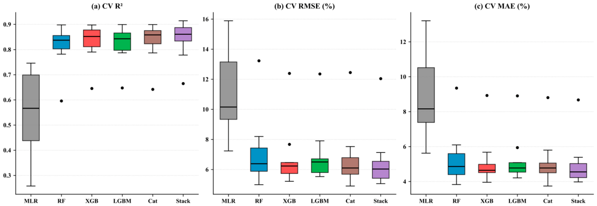
Figure A2.
Learning curves for the Random Forest model of the 2020→2025 relative change in summer PM2.5 (%): Mean R2 across five spatial GroupKFold folds at each training-subset size (shaded bands: ±1 standard deviation). Blue: Training R2; orange: Spatially cross-validated R2, which is negative below ≈1600 training cells and reaches 0.80 at the maximum size.
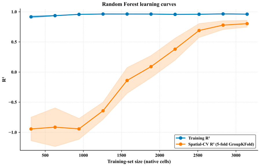
Figure A3.
Spatial distribution of cross-validated residuals (GEOS-CF reference minus estimated, %) of the 2020→2025 relative change in summer PM2.5 for the Random Forest model over the Arabian Peninsula (native 0.25° grid). Blue tones indicate negative residuals (overestimation); red tones indicate positive residuals (underestimation); the diverging color scale is centered at zero. The residual clusters shown here define the subregional strata of Table 3.
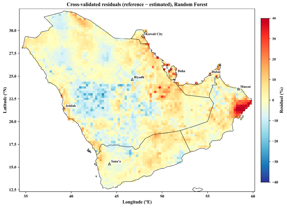
Figure A4.
Consensus feature-importance ranking for the Random Forest model of the 2020→2025 relative change in summer PM2.5 (%). The consensus rank of each predictor is the arithmetic mean of the ordinal ranks assigned by mean decrease in impurity (MDI), permutation importance (ΔR2), and mean absolute SHAP value; lower values indicate higher overall importance. Error bars denote the range of ranks across the three methods. These metrics quantify predictive association within the fitted model, not physical causation.
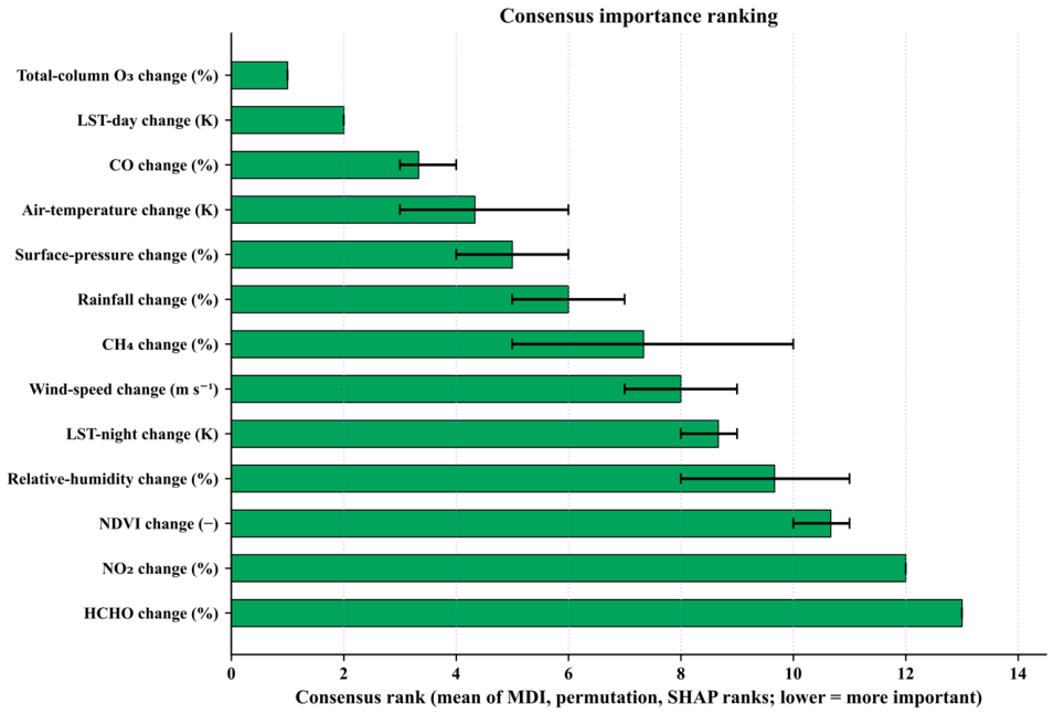
Figure A5.
SHAP beeswarm summary plot for the Random Forest model of the 2020→2025 relative change in summer PM2.5 (%). Each point represents one native cell; horizontal position indicates the SHAP value (contribution to the estimated change, %). Point color encodes the standardized predictor value (blue: low; red: high). Features are ordered from top to bottom by decreasing mean |SHAP| value.
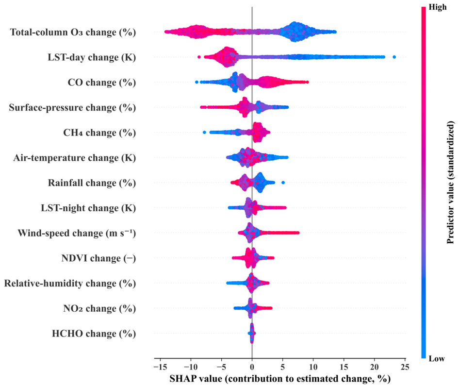
Figure A6.
SHAP dependence plots for the three highest-ranked predictors of the 2020→2025 relative change in summer PM2.5 (%): (a) Total-column O3 change, (b) daytime-LST change, and (c) CO change. Each point represents one native cell; the x-axis shows the standardized predictor value and the y-axis the corresponding SHAP contribution (%); the black curve is a Savitzky–Golay smoothed trend. Point color encodes the value of the most strongly interacting secondary feature, identified by the maximum SHAP interaction value. The O3 dependence is a decreasing step and the LST-day dependence is decreasing, with large positive contributions where the daytime surface cooled between 2020 and 2025.
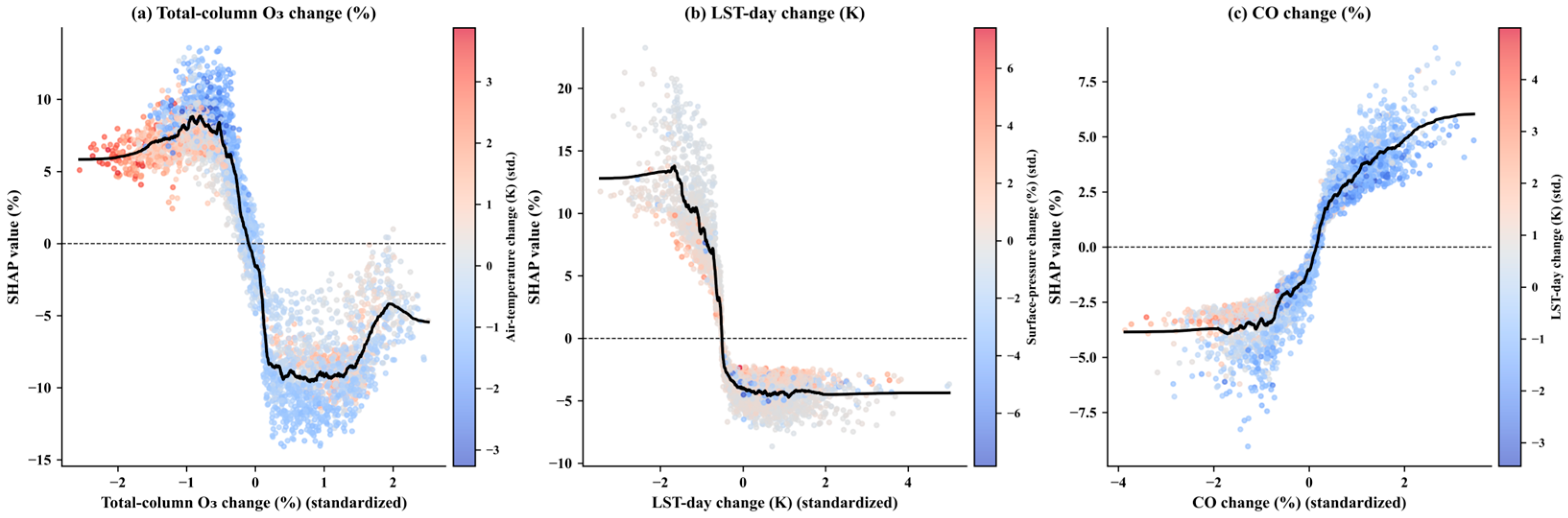
Figure A7.
Partial-dependence plots for the six top-ranked predictors of the 2020→2025 relative change in summer PM2.5 (%), as determined by consensus importance rank. Each panel shows the marginal effect of a single predictor on the Random Forest output, with all other predictors held at their observed values. Predictor values are in standardized units (mean = 0, SD = 1).
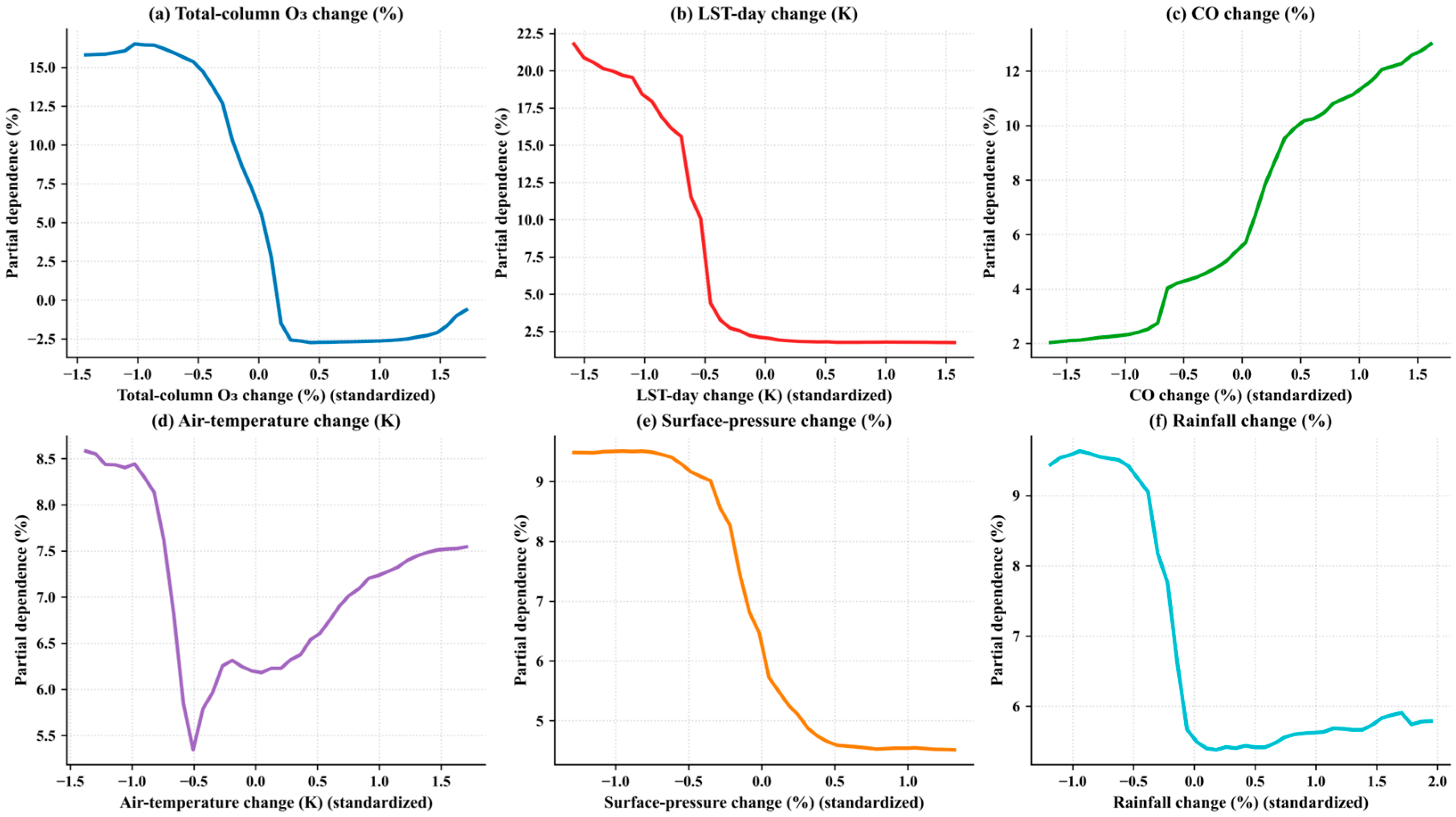
Figure A8.
Split-conformal 90% prediction intervals for rotation 1 of the three-way spatial design (Table A4): A Random Forest trained on outer folds 1–6, calibrated on folds 7–8, and tested on folds 9–10 (n = 788 test cells, which include 49 of the 51 extreme-cluster cells). Test cells are sorted in ascending order of estimated change along the x-axis. The solid blue line denotes the estimated change; the band bounded by dashed red lines indicates the 90% interval derived from the calibration-residual quantiles (q0.05 and q0.95); black dots are GEOS-CF reference values (modeled, not surface observations). Coverage, interval width, and the share of extreme cells covered are annotated.
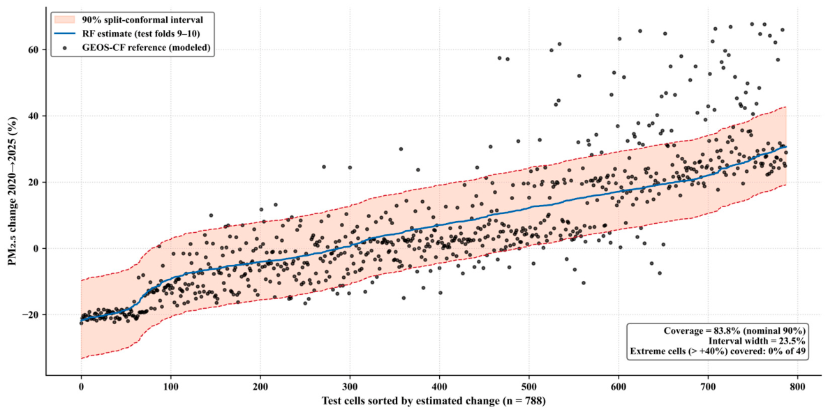
Figure A9.
Empirical semivariogram of the 2020→2025 relative change in summer PM2.5 of the GEOS-CF reference, computed from a random subsample of 2500 native cells (planar-approximated distances; 50 km lag bins). The dashed red line marks the field variance (≈305%2); the shaded bands mark the dimensions of the 10 × 10 blocks (≈214–255 km) and of the 5 × 5 blocks (≈427–511 km). Semivariance rises monotonically across all resolvable lags, reaching about 22% of the field variance at the 10 × 10 block dimension, one half near ≈575 km, and the field variance only near ≈975 km, without a clear sill—the signature of basin-scale organization dominated by the east–west dipole (Figure 5). No feasible block size therefore isolates validation cells from spatially dependent training cells, which motivates the transfer diagnostics of Section 2.12 and Section 3.6.
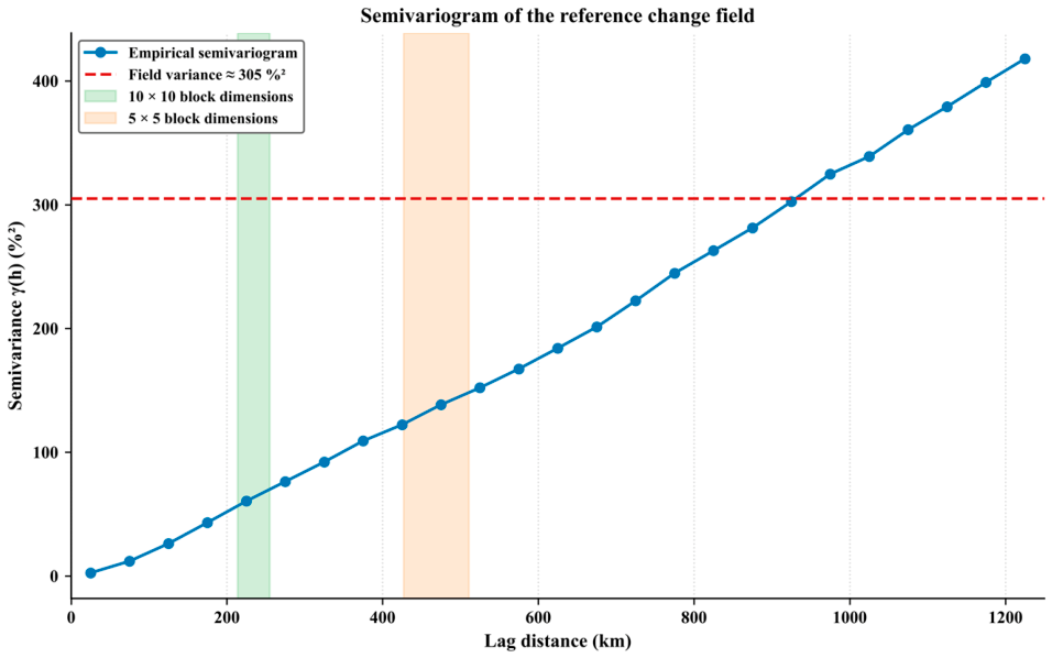
References
- Murray, C.J.L.; Aravkin, A.Y.; Zheng, P.; Abbafati, C.; Abbas, K.M.; Abbasi-Kangevari, M.; Abd-Allah, F.; Abdelalim, A.; Abdollahi, M.; Abdollahpour, I.; et al. Global Burden of 87 Risk Factors in 204 Countries and Territories, 1990–2019: A Systematic Analysis for the Global Burden of Disease Study 2019. Lancet 2020, 396, 1223–1249. [Google Scholar] [CrossRef] [Scilit] [PubMed]
- Boucher, O.; Randall, D.; Artaxo, P.; Bretherton, C.; Feingold, G.; Forster, P.; Kerminen, V.M.; Kondo, Y.; Liao, H.; Lohmann, U.; et al. Clouds and Aerosols. In Climate Change 2013: The Physical Science Basis. Contribution of Working Group I to the Fifth Assessment Report of the Intergovernmental Panel on Climate Change; Stocker, T.F., Qin, D., Plattner, G.-K., Tignor, M., Allen, S.K., Boschung, J., Nauels, A., Xia, Y., Bex, V., Midgley, P.M., Eds.; Cambridge University Press: Cambridge, UK; New York, NY, USA, 2013; pp. 571–657. [Google Scholar]
- Prospero, J.M.; Ginoux, P.; Torres, O.; Nicholson, S.E.; Gill, T.E. Environmental Characterization of Global Sources of Atmospheric Soil Dust Identified with the Nimbus 7 Total Ozone Mapping Spectrometer (TOMS) Absorbing Aerosol Product. Rev. Geophys. 2002, 40, 1002. [Google Scholar] [CrossRef] [Scilit]
- Lelieveld, J.; Hadjinicolaou, P.; Kostopoulou, E.; Chenoweth, J.; El Maayar, M.; Giannakopoulos, C.; Hannides, C.; Lange, M.A.; Tanarhte, M.; Tyrlis, E.; et al. Climate Change and Impacts in the Eastern Mediterranean and the Middle East. Clim. Change 2012, 114, 667–687. [Google Scholar] [CrossRef] [Scilit] [PubMed]
- Alkhodaidi, A.; Hakeem, A.; Attiah, A.; Mhawish, A.; Almakky, A. Air Pollutant PM10 Estimation in Saudi Arabia Using Machine Learning. AIMS Environ. Sci. 2026, 13, 126–158. [Google Scholar] [CrossRef] [Scilit]
- Martin, R.V. Satellite Remote Sensing of Surface Air Quality. Atmos. Environ. 2008, 42, 7823–7843. [Google Scholar] [CrossRef] [Scilit]
- Veefkind, J.P.; Aben, I.; McMullan, K.; Förster, H.; de Vries, J.; Otter, G.; Claas, J.; Eskes, H.J.; De Haan, J.F.; Kleipool, Q.; et al. TROPOMI on the ESA Sentinel-5 Precursor: A GMES Mission for Global Observations of the Atmospheric Composition for Climate, Air Quality and Ozone Layer Applications. Remote Sens. Environ. 2012, 120, 70–83. [Google Scholar] [CrossRef] [Scilit]
- Keller, C.A.; Knowland, K.E.; Duncan, B.N.; Liu, J.; Anderson, D.C.; Das, S.; Lucchesi, R.A.; Lundgren, E.W.; Nicely, J.M.; Nielsen, E.; et al. Description of the NASA GEOS Composition Forecast Modeling System GEOS-CF v1.0. J. Adv. Model. Earth Syst. 2021, 13, e2020MS002413. [Google Scholar] [CrossRef] [Scilit] [PubMed]
- Hamdi, I.M.; Hanai, A.A.; Aldohan, A.; Albalawi, E.; Al-Absi, S.; Youssef, Y.M. Air Quality Variations over the Arabian Peninsula during the Post-COVID-19 Lockdown: Satellite-Derived Trends Using Sentinel-5P TROPOMI and NASA GEOS-CF. Adv. Space Res. 2026, 78, 8909–8927. [Google Scholar] [CrossRef] [Scilit]
- Wan, Z.; Hook, S.; Hulley, G. MYD11A1 MODIS/Aqua Land Surface Temperature/Emissivity Daily L3 Global 1 km SIN Grid V061; NASA EOSDIS Land Processes DAAC: Sioux Falls, SD, USA, 2021. [Google Scholar] [CrossRef]
- Didan, K. MYD13Q1 MODIS/Aqua Vegetation Indices 16-Day L3 Global 250 m SIN Grid V061; NASA EOSDIS Land Processes DAAC: Sioux Falls, SD, USA, 2021. [Google Scholar] [CrossRef]
- Abbas, W.; Hamdi, I. Satellite-Based Discrimination of Urban Dynamics-Induced Local Bias from Day/Night Temperature Trends across the Nile Delta, Egypt: A Basis for Climate Change Impacts Assessment. Sustainability 2022, 14, 14510. [Google Scholar] [CrossRef] [Scilit]
- Hamdi, I.; Fawzy, M.; Zelenakova, M.; Abbas, W. Heat Island Dynamics and Heat Stress Implications on the Population of El-Mansourah Conurbation, Egypt: Temporal and Proposed Solutions Using MODIS Imagery and ENVI-met Simulation. Geomat. Nat. Hazards Risk 2024, 15, 2291328. [Google Scholar] [CrossRef] [Scilit]
- Nahas, F.; Hamdi, I.; Hereher, M.; Zelenakova, M.; El Kenawy, A.M. Warming Trends in the Nile Delta: A High-Resolution Spatial Statistical Approach. Remote Sens. Appl. Soc. Environ. 2025, 37, 101408. [Google Scholar] [CrossRef] [Scilit]
- Hamdi, I.M. Fine-Scale Urban Heat Mapping by Machine Learning Downscaling of MODIS Land Surface Temperature in a Hyper-Arid Megacity. Sustain. Cities Soc. 2026, 150, 107878. [Google Scholar] [CrossRef] [Scilit]
- Youssef, Y.M.; Đurin, B.; Alturki, A.A.; Šrajbek, M.; Hamdi, I.M. Two Decades of Optical and Thermal Variability in Lake Nasser: A Multi-Variable MODIS Assessment on a 5 km Analysis Grid (2005–2025). Water 2026, 18, 2213. [Google Scholar] [CrossRef] [Scilit]
- Muñoz-Sabater, J.; Dutra, E.; Agustí-Panareda, A.; Albergel, C.; Arduini, G.; Balsamo, G.; Boussetta, S.; Choulga, M.; Harrigan, S.; Hersbach, H.; et al. ERA5-Land: A State-of-the-Art Global Reanalysis Dataset for Land Applications. Earth Syst. Sci. Data 2021, 13, 4349–4383. [Google Scholar] [CrossRef] [Scilit]
- Chen, G.; Li, S.; Knibbs, L.D.; Hamm, N.A.S.; Cao, W.; Li, T.; Guo, J.; Ren, H.; Abramson, M.J.; Guo, Y. A Machine Learning Method to Estimate PM2.5 Concentrations across China with Remote Sensing, Meteorological and Land Use Information. Sci. Total Environ. 2018, 636, 52–60. [Google Scholar] [CrossRef] [Scilit] [PubMed]
- Zamani Joharestani, M.; Cao, C.; Ni, X.; Bashir, B.; Talebiesfandarani, S. PM2.5 Prediction Based on Random Forest, XGBoost, and Deep Learning Using Multisource Remote Sensing Data. Atmosphere 2019, 10, 373. [Google Scholar] [CrossRef] [Scilit]
- Hamdi, I.M.; Albalawi, E.; AbdAlmapoed, E.K.; AbdElaal, S.R. Mitigating Surface Industrial Heat Island Effects in Arid Environments: A Machine Learning Approach to Sustainable Planning. Energy Build. 2026, 361, 117449. [Google Scholar] [CrossRef] [Scilit]
- Roberts, D.R.; Bahn, V.; Ciuti, S.; Boyce, M.S.; Elith, J.; Guillera-Arroita, G.; Hauenstein, S.; Lahoz-Monfort, J.J.; Schröder, B.; Thuiller, W.; et al. Cross-Validation Strategies for Data with Temporal, Spatial, Hierarchical, or Phylogenetic Structure. Ecography 2017, 40, 913–929. [Google Scholar] [CrossRef] [Scilit]
- Schratz, P.; Muenchow, J.; Iturritxa, E.; Richter, J.; Brenning, A. Hyperparameter Tuning and Performance Assessment of Statistical and Machine-Learning Algorithms Using Spatial Data. Ecol. Model. 2019, 406, 109–120. [Google Scholar] [CrossRef] [Scilit]
- Ploton, P.; Mortier, F.; Réjou-Méchain, M.; Barbier, N.; Picard, N.; Rossi, V.; Dormann, C.; Cornu, G.; Viennois, G.; Bayol, N.; et al. Spatial Validation Reveals Poor Predictive Performance of Large-Scale Ecological Mapping Models. Nat. Commun. 2020, 11, 4540. [Google Scholar] [CrossRef] [Scilit] [PubMed]
- Meyer, H.; Pebesma, E. Predicting into Unknown Space? Estimating the Area of Applicability of Spatial Prediction Models. Methods Ecol. Evol. 2021, 12, 1620–1633. [Google Scholar] [CrossRef] [Scilit]
- Daniyal, M.; Alyami, H.; Alqahtani, A.J.; Talha, M.; Rahman, A.; Al Mutair, A. Modeling and Forecasting Air Pollution for Public Health Protection Based on ML and Time Series Models in Gulf Cooperation Council (GCC) Countries. BMC Public Health 2026, 26, 280. [Google Scholar] [CrossRef] [Scilit] [PubMed]
- Lundberg, S.M.; Lee, S.-I. A Unified Approach to Interpreting Model Predictions. In Advances in Neural Information Processing Systems 30; Guyon, I., Luxburg, U.V., Bengio, S., Wallach, H., Fergus, R., Vishwanathan, S., Garnett, R., Eds.; Curran Associates: Red Hook, NY, USA, 2017; pp. 4765–4774. [Google Scholar]
- Angelopoulos, A.N.; Bates, S. Conformal Prediction: A Gentle Introduction. Found. Trends Mach. Learn. 2023, 16, 494–591. [Google Scholar] [CrossRef] [Scilit]
- Yu, Y.; Notaro, M.; Liu, Z.; Wang, F.; Alkolibi, F.; Fadda, E.; Bakhrjy, F. Climatic Controls on the Interannual to Decadal Variability in Saudi Arabian Dust Activity: Toward the Development of a Seasonal Dust Prediction Model. J. Geophys. Res. Atmos. 2015, 120, 1739–1758. [Google Scholar] [CrossRef] [Scilit]
- Jish Prakash, P.; Stenchikov, G.; Kalenderski, S.; Osipov, S.; Bangalath, H. The Impact of Dust Storms on the Arabian Peninsula and the Red Sea. Atmos. Chem. Phys. 2015, 15, 199–222. [Google Scholar] [CrossRef] [Scilit]
- Francis, D.; Fonseca, R.; Nelli, N.; Teixido, O.; Mohamed, R.; Perry, R. Increased Shamal Winds and Dust Activity over the Arabian Peninsula during the COVID-19 Lockdown Period in 2020. Aeolian Res. 2022, 55, 100786. [Google Scholar] [CrossRef] [Scilit] [PubMed]
- Meyer, H.; Pebesma, E. Machine Learning-Based Global Maps of Ecological Variables and the Challenge of Assessing Them. Nat. Commun. 2022, 13, 2208. [Google Scholar] [CrossRef] [Scilit] [PubMed]
- Wadoux, A.M.J.-C.; Heuvelink, G.B.M.; de Bruin, S.; Brus, D.J. Spatial Cross-Validation Is Not the Right Way to Evaluate Map Accuracy. Ecol. Model. 2021, 457, 109692. [Google Scholar] [CrossRef] [Scilit]
- Al-Hemoud, A.; Al-Dashti, H.; Al-Saleh, A.; Petrov, P.; Malek, M.; Elhamoud, E.; Al-Khafaji, S.; Li, J.; Koutrakis, P.; Doronzo, D.; et al. Dust Storm “Hot Spots” and Transport Pathways Affecting the Arabian Peninsula. J. Atmos. Sol.-Terr. Phys. 2022, 238–239, 105932. [Google Scholar] [CrossRef] [Scilit]
- Gorelick, N.; Hancher, M.; Dixon, M.; Ilyushchenko, S.; Thau, D.; Moore, R. Google Earth Engine: Planetary-Scale Geospatial Analysis for Everyone. Remote Sens. Environ. 2017, 202, 18–27. [Google Scholar] [CrossRef] [Scilit]
- Hamdi, I.; AbdAlmapoed, E.K.; AbdElaal, S.R. Assessment of Urban Heat Island Effects in Industrial Areas of Egypt Using Robust Statistical Methods. Remote Sens. Appl. Soc. Environ. 2025, 40, 101777. [Google Scholar] [CrossRef] [Scilit]
- Garane, K.; Koukouli, M.-E.; Verhoelst, T.; Lerot, C.; Heue, K.-P.; Fioletov, V.; Balis, D.; Bais, A.; Bazureau, A.; Dehn, A.; et al. TROPOMI/S5P Total Ozone Column Data: Global Ground-Based Validation and Consistency with Other Satellite Missions. Atmos. Meas. Tech. 2019, 12, 5263–5287. [Google Scholar] [CrossRef] [Scilit]
- Funk, C.; Peterson, P.; Landsfeld, M.; Pedreros, D.; Verdin, J.; Shukla, S.; Husak, G.; Rowland, J.; Harrison, L.; Hoell, A.; et al. The Climate Hazards Infrared Precipitation with Stations—A New Environmental Record for Monitoring Extremes. Sci. Data 2015, 2, 150066. [Google Scholar] [CrossRef] [Scilit] [PubMed]
- Duan, Z.; Liu, J.; Tuo, Y.; Chiogna, G.; Disse, M. Evaluation of Eight High Spatial Resolution Gridded Precipitation Products in Adige Basin (Italy) at Multiple Temporal and Spatial Scales. Sci. Total Environ. 2016, 573, 1536–1553. [Google Scholar] [CrossRef] [Scilit] [PubMed]
- van Donkelaar, A.; Martin, R.V.; Brauer, M.; Kahn, R.; Levy, R.; Verduzco, C.; Villeneuve, P.J. Global Estimates of Ambient Fine Particulate Matter Concentrations from Satellite-Based Aerosol Optical Depth: Development and Application. Environ. Health Perspect. 2010, 118, 847–855. [Google Scholar] [CrossRef] [Scilit] [PubMed]
- Hsu, N.C.; Jeong, M.-J.; Bettenhausen, C.; Sayer, A.M.; Hansell, R.; Seftor, C.S.; Huang, J.; Tsay, S.-C. Enhanced Deep Blue Aerosol Retrieval Algorithm: The Second Generation. J. Geophys. Res. Atmos. 2013, 118, 9296–9315. [Google Scholar] [CrossRef] [Scilit]
- Theys, N.; De Smedt, I.; Yu, H.; Danckaert, T.; van Gent, J.; Hörmann, C.; Wagner, T.; Hedelt, P.; Bauer, H.; Romahn, F.; et al. Sulfur Dioxide Retrievals from TROPOMI Onboard Sentinel-5 Precursor: Algorithm Theoretical Basis. Atmos. Meas. Tech. 2017, 10, 119–153. [Google Scholar] [CrossRef] [Scilit]
- Breiman, L. Random Forests. Mach. Learn. 2001, 45, 5–32. [Google Scholar] [CrossRef] [Scilit]
- Chen, T.; Guestrin, C. XGBoost: A Scalable Tree Boosting System. In Proceedings of the 22nd ACM SIGKDD International Conference on Knowledge Discovery and Data Mining, San Francisco, CA, USA, 13–17 August 2016; pp. 785–794. [Google Scholar] [CrossRef] [Scilit]
- Ke, G.; Meng, Q.; Finley, T.; Wang, T.; Chen, W.; Ma, W.; Ye, Q.; Liu, T.-Y. LightGBM: A Highly Efficient Gradient Boosting Decision Tree. In Advances in Neural Information Processing Systems 30; Guyon, I., Luxburg, U.V., Bengio, S., Wallach, H., Fergus, R., Vishwanathan, S., Garnett, R., Eds.; Curran Associates: Red Hook, NY, USA, 2017; pp. 3146–3154. [Google Scholar]
- Prokhorenkova, L.; Gusev, G.; Vorobev, A.; Dorogush, A.V.; Gulin, A. CatBoost: Unbiased Boosting with Categorical Features. In Advances in Neural Information Processing Systems 31; Bengio, S., Wallach, H., Larochelle, H., Grauman, K., Cesa-Bianchi, N., Garnett, R., Eds.; Curran Associates: Red Hook, NY, USA, 2018; pp. 6638–6648. [Google Scholar]
- Nash, J.E.; Sutcliffe, J.V. River Flow Forecasting through Conceptual Models Part I—A Discussion of Principles. J. Hydrol. 1970, 10, 282–290. [Google Scholar] [CrossRef] [Scilit]
- Krause, P.; Boyle, D.P.; Bäse, F. Comparison of Different Efficiency Criteria for Hydrological Model Assessment. Adv. Geosci. 2005, 5, 89–97. [Google Scholar] [CrossRef] [Scilit]
- Strobl, C.; Boulesteix, A.-L.; Zeileis, A.; Hothorn, T. Bias in Random Forest Variable Importance Measures: Illustrations, Sources and a Solution. BMC Bioinform. 2007, 8, 25. [Google Scholar] [CrossRef] [Scilit] [PubMed]
- Rey, S.J.; Anselin, L. PySAL: A Python Library of Spatial Analytical Methods. In Handbook of Applied Spatial Analysis: Software Tools, Methods and Applications; Fischer, M.M., Getis, A., Eds.; Springer: Berlin/Heidelberg, Germany, 2010; pp. 175–193. [Google Scholar] [CrossRef] [Scilit] [PubMed]
- Vovk, V.; Gammerman, A.; Shafer, G. Algorithmic Learning in a Random World; Springer: New York, NY, USA, 2005. [Google Scholar]
- Barber, R.F.; Candès, E.J.; Ramdas, A.; Tibshirani, R.J. Conformal Prediction beyond Exchangeability. Ann. Stat. 2023, 51, 816–845. [Google Scholar] [CrossRef] [Scilit]
- Alowfi, S.; Hamdi, I.; Selín, J.; Aldohan, A.; Zeleňáková, M.; Dąbrowska, D.; Youssef, Y. Satellite-Based Assessment of Chlorophyll-a Variability, Seasonal Trends, and Eutrophication Risk for Water Sustainability in a Strategic Desert Reservoir. Water 2026, 18, 2256. [Google Scholar] [CrossRef] [Scilit]
- Alghamdi, M.A.; Khoder, M.; Harrison, R.M.; Hyvärinen, A.-P.; Hussein, T.; Al-Jeelani, H.; Abdelmaksoud, A.S.; Goknil, M.H.; Shabbaj, I.I.; Almehmadi, F.M.; et al. Temporal Variations of O3 and NOx in the Urban Background Atmosphere of the Coastal City Jeddah, Saudi Arabia. Atmos. Environ. 2014, 94, 205–214. [Google Scholar] [CrossRef] [Scilit]
- Khalil, M.A.K. Steady States and Transport Processes in Urban Ozone Balances. npj Clim. Atmos. Sci. 2018, 1, 22. [Google Scholar] [CrossRef] [Scilit]
- Kalenderski, S.; Stenchikov, G. High-Resolution Regional Modeling of Summertime Transport and Impact of African Dust over the Red Sea and Arabian Peninsula. J. Geophys. Res. Atmos. 2016, 121, 6435–6458. [Google Scholar] [CrossRef] [Scilit]
- Anil, I.; Alagha, O. The Impact of COVID-19 Lockdown on the Air Quality of Eastern Province, Saudi Arabia. Air Qual. Atmos. Health 2021, 14, 117–128. [Google Scholar] [CrossRef] [Scilit] [PubMed]
- Ukhov, A.; Mostamandi, S.; da Silva, A.; Flemming, J.; Alshehri, Y.; Shevchenko, I.; Stenchikov, G. Assessment of Natural and Anthropogenic Aerosol Air Pollution in the Middle East Using MERRA-2, CAMS Data Assimilation Products, and High-Resolution WRF-Chem Model Simulations. Atmos. Chem. Phys. 2020, 20, 9281–9310. [Google Scholar] [CrossRef] [Scilit]
- Abdelsattar, A.; Al Nadhairi, R.; Hassan, A.N. Space-Based Monitoring of NO2 Levels during COVID-19 Lockdown in Cairo, Egypt and Riyadh, Saudi Arabia. Egypt. J. Remote Sens. Space Sci. 2021, 24, 659–664. [Google Scholar] [CrossRef] [Scilit]
- Grange, S.K.; Lee, J.D.; Drysdale, W.S.; Lewis, A.C.; Hueglin, C.; Emmenegger, L.; Carslaw, D.C. COVID-19 Lockdowns Highlight a Risk of Increasing Ozone Pollution in European Urban Areas. Atmos. Chem. Phys. 2021, 21, 4169–4185. [Google Scholar] [CrossRef] [Scilit]
- Dantas, G.; Siciliano, B.; França, B.B.; da Silva, C.M.; Arbilla, G. The Impact of COVID-19 Partial Lockdown on the Air Quality of the City of Rio de Janeiro, Brazil. Sci. Total Environ. 2020, 729, 139085. [Google Scholar] [CrossRef] [Scilit] [PubMed]
- Al Yammahi, A.; Aung, Z. A Study of Nitrogen Dioxide (NO2) Periodicity over the United Arab Emirates Using Wavelet Analysis. Sci. Rep. 2022, 12, 18144. [Google Scholar] [CrossRef] [Scilit] [PubMed]
- Barkley, M.P.; González Abad, G.; Kurosu, T.P.; Spurr, R.; Torbatian, S.; Lerot, C. OMI Air-Quality Monitoring over the Middle East. Atmos. Chem. Phys. 2017, 17, 4687–4709. [Google Scholar] [CrossRef] [Scilit]
- Chen, Z.; Jacob, D.J.; Gautam, R.; Omara, M.; Stavins, R.N.; Stowe, R.C.; Nesser, H.; Sulprizio, M.P.; Lorente, A.; Varon, D.J.; et al. Satellite Quantification of Methane Emissions and Oil–Gas Methane Intensities from Individual Countries in the Middle East and North Africa: Implications for Climate Action. Atmos. Chem. Phys. 2023, 23, 5945–5967. [Google Scholar] [CrossRef] [Scilit]
- Hammam, E.E.; Al Ghamdi, M.A.; Almazroui, M.; Hassan, I.A. The COVID-19 Pandemic: Quantification of Temporal Variations in Air Pollutants before, during and Post the Lockdown in Jeddah City, Saudi Arabia. Earth Syst. Environ. 2022, 6, 917–926. [Google Scholar] [CrossRef] [Scilit] [PubMed]
- Rocha-Lima, A.; Colarco, P.R.; Darmenov, A.S.; Nowottnick, E.P.; da Silva, A.M.; Oman, L.D. Investigation of Observed Dust Trends over the Middle East Region in NASA Goddard Earth Observing System (GEOS) Model Simulations. Atmos. Chem. Phys. 2024, 24, 2443–2464. [Google Scholar] [CrossRef] [Scilit]
- Farahat, A.; El-Askary, H.; Adetokunbo, P.; Fuad, A.T. Analysis of Aerosol Absorption Properties and Transport over North Africa and the Middle East Using AERONET Data. Ann. Geophys. 2016, 34, 1031–1044. [Google Scholar] [CrossRef] [Scilit]
- Akasha, H.; Ghaffarpasand, O.; Pope, F.D. Climate Change, Air Pollution and the Associated Burden of Disease in the Arabian Peninsula and Neighbouring Regions: A Critical Review of the Literature. Sustainability 2023, 15, 3766. [Google Scholar] [CrossRef] [Scilit]
- Dienhart, D.; Crowley, J.N.; Bourtsoukidis, E.; Edtbauer, A.; Eger, P.G.; Ernle, L.; Harder, H.; Hottmann, B.; Martinez, M.; Parchatka, U.; et al. Measurement Report: Observation-Based Formaldehyde Production Rates and Their Relation to OH Reactivity around the Arabian Peninsula. Atmos. Chem. Phys. 2021, 21, 17373–17388. [Google Scholar] [CrossRef] [Scilit]
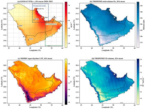
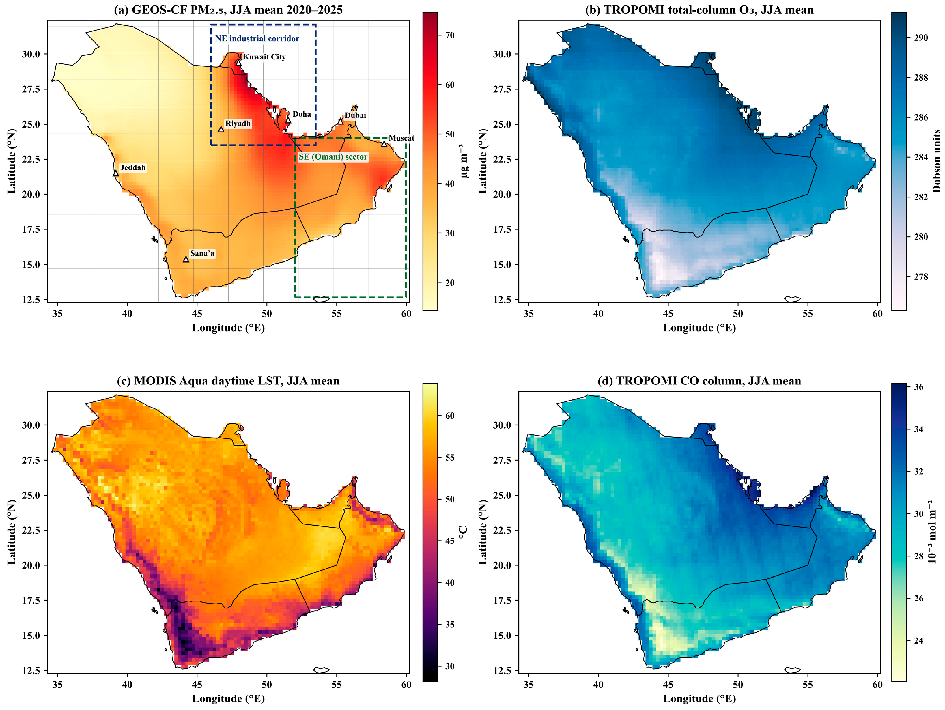
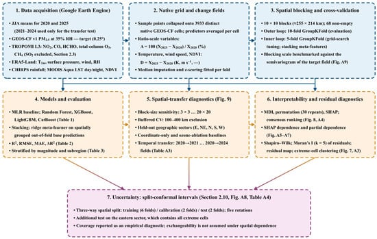
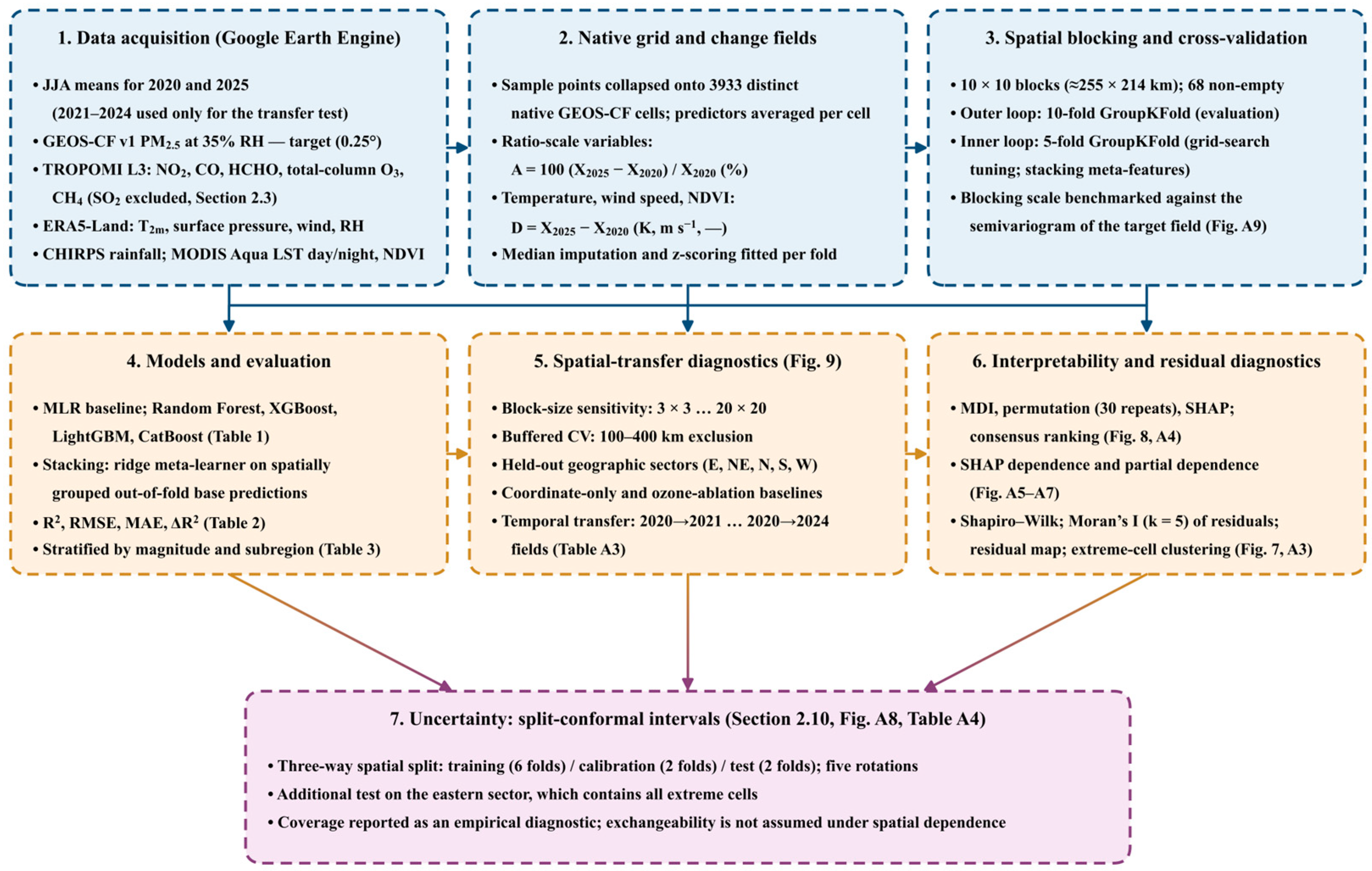
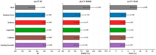
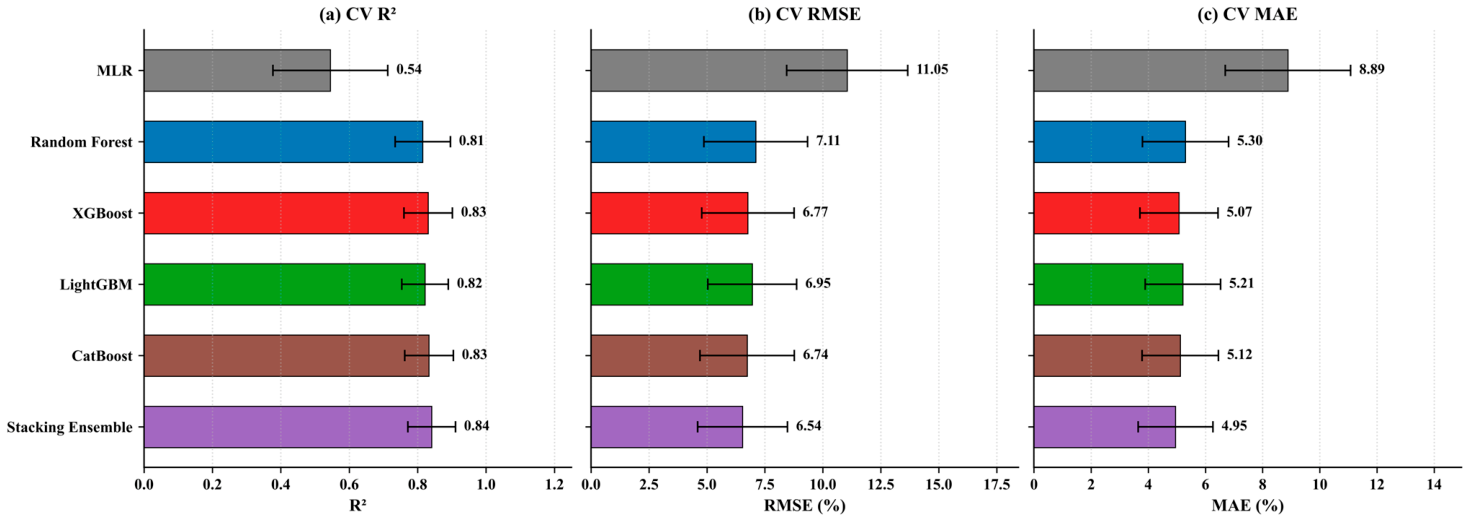
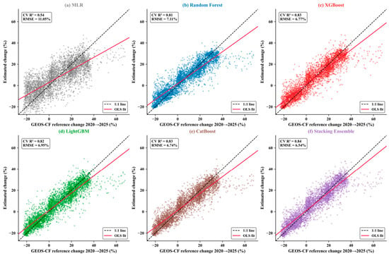
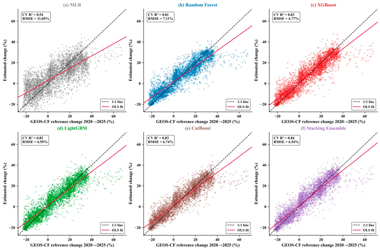
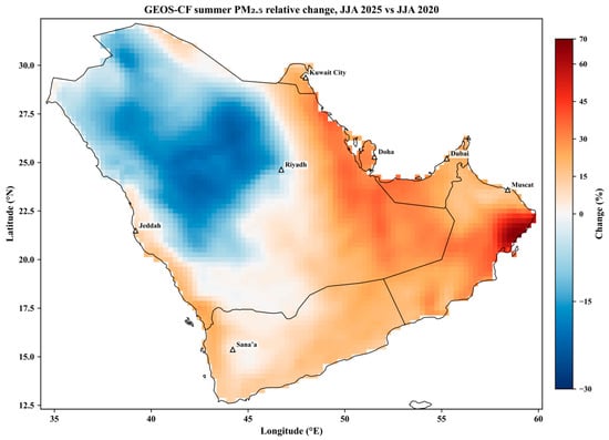
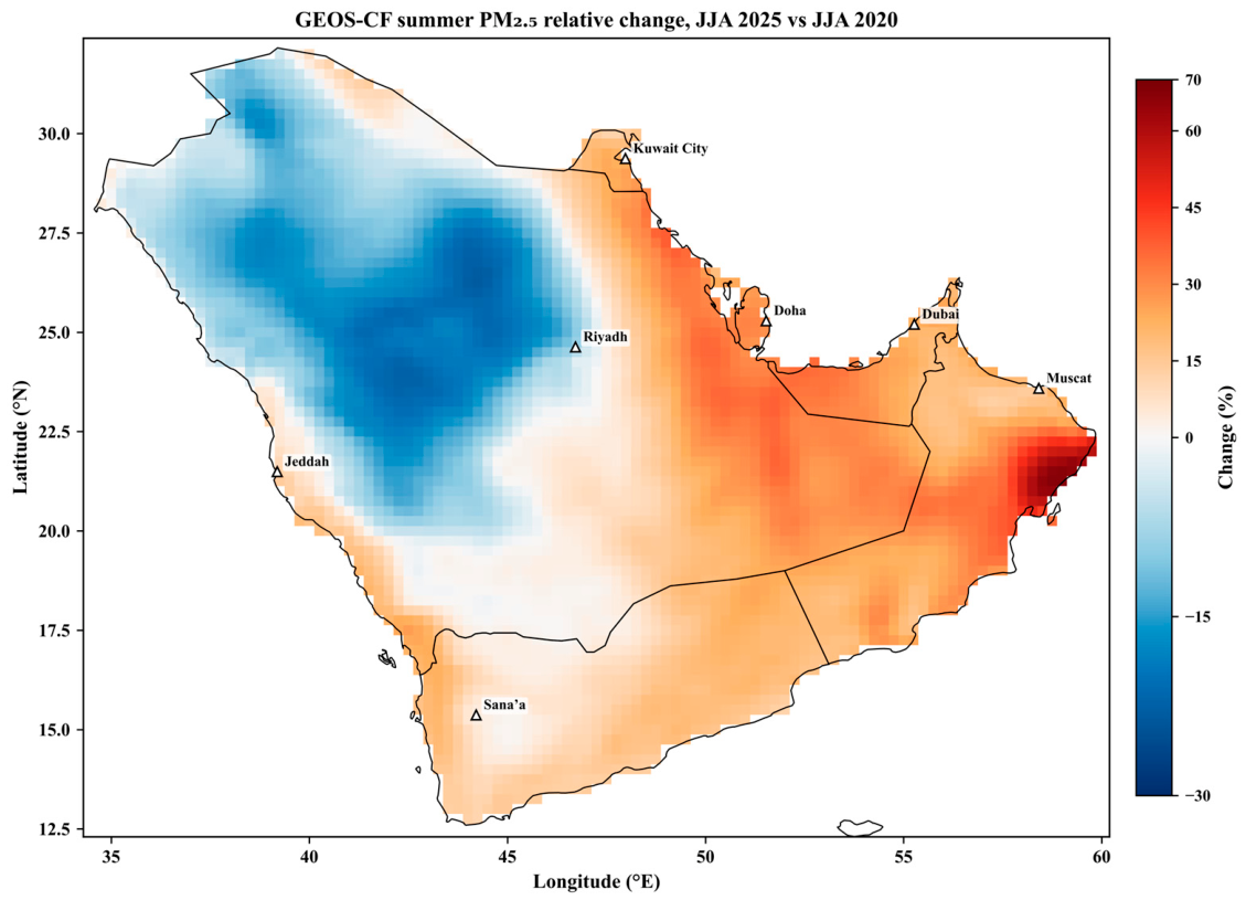
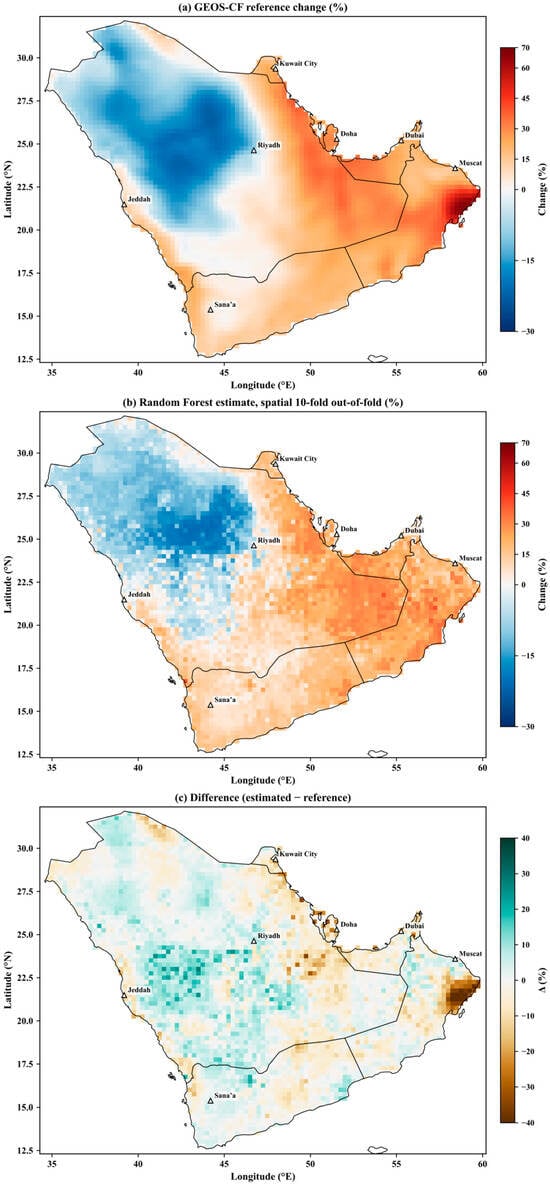
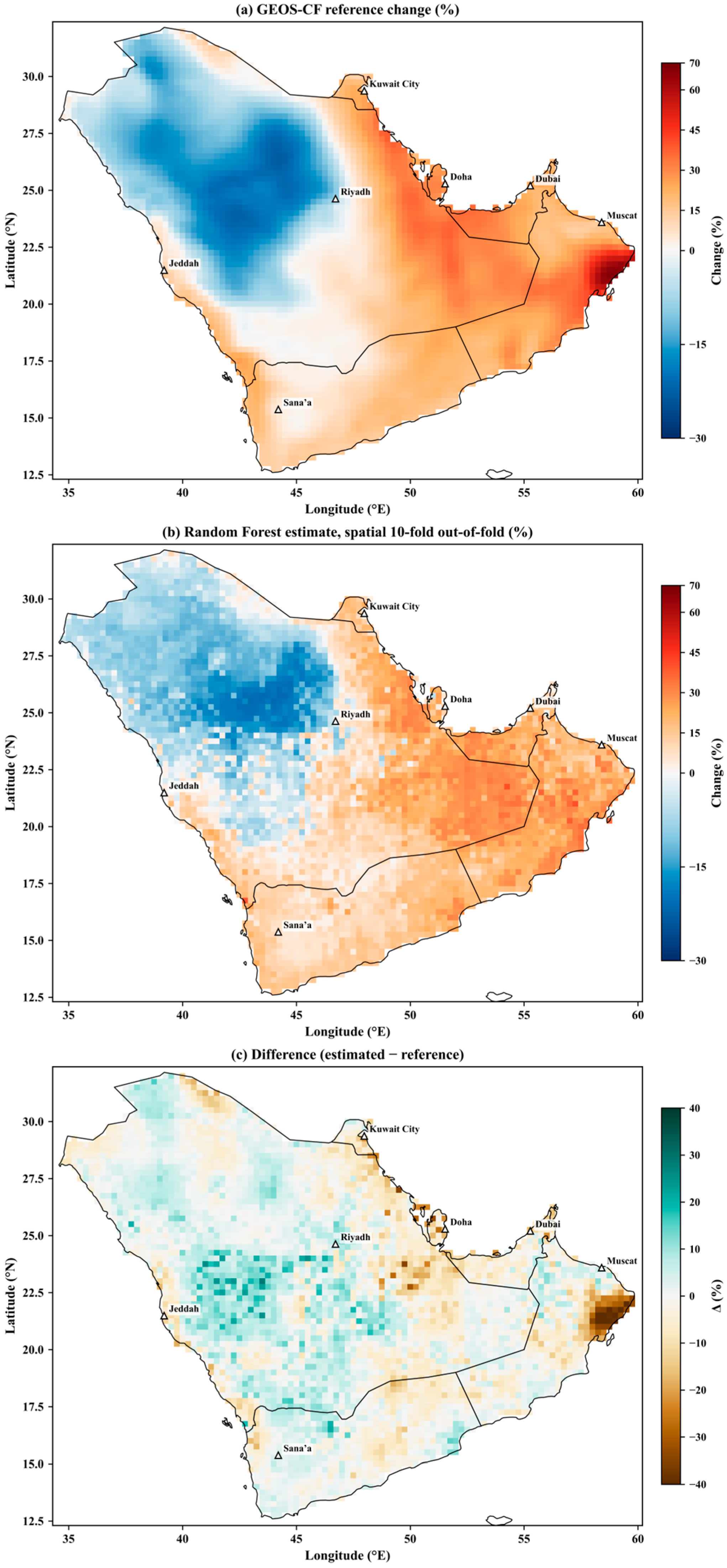
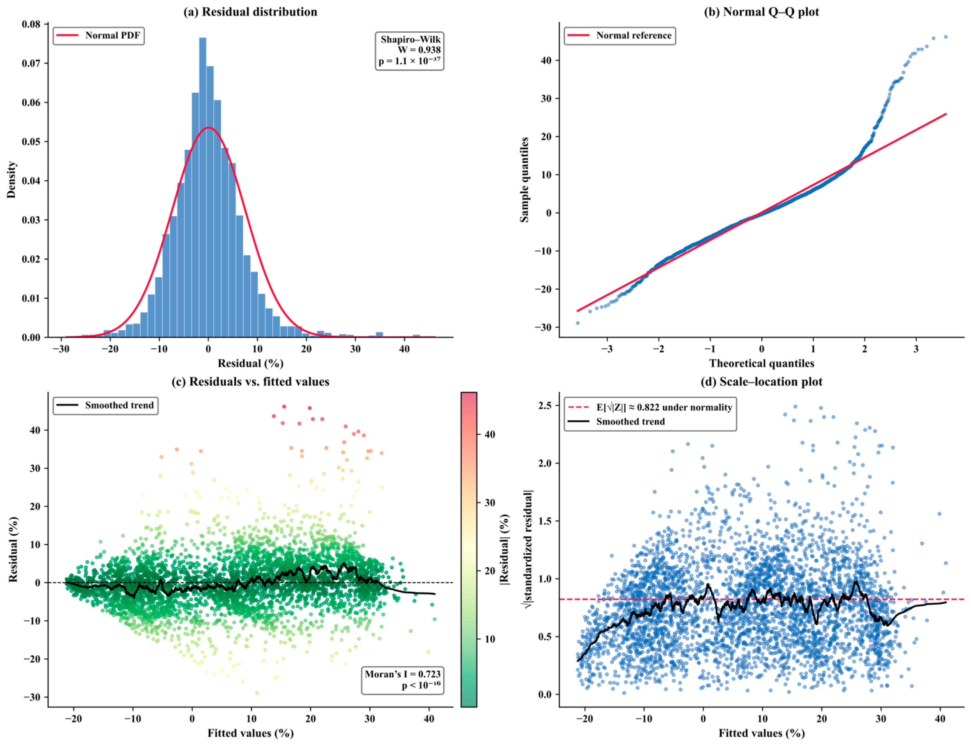
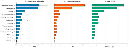
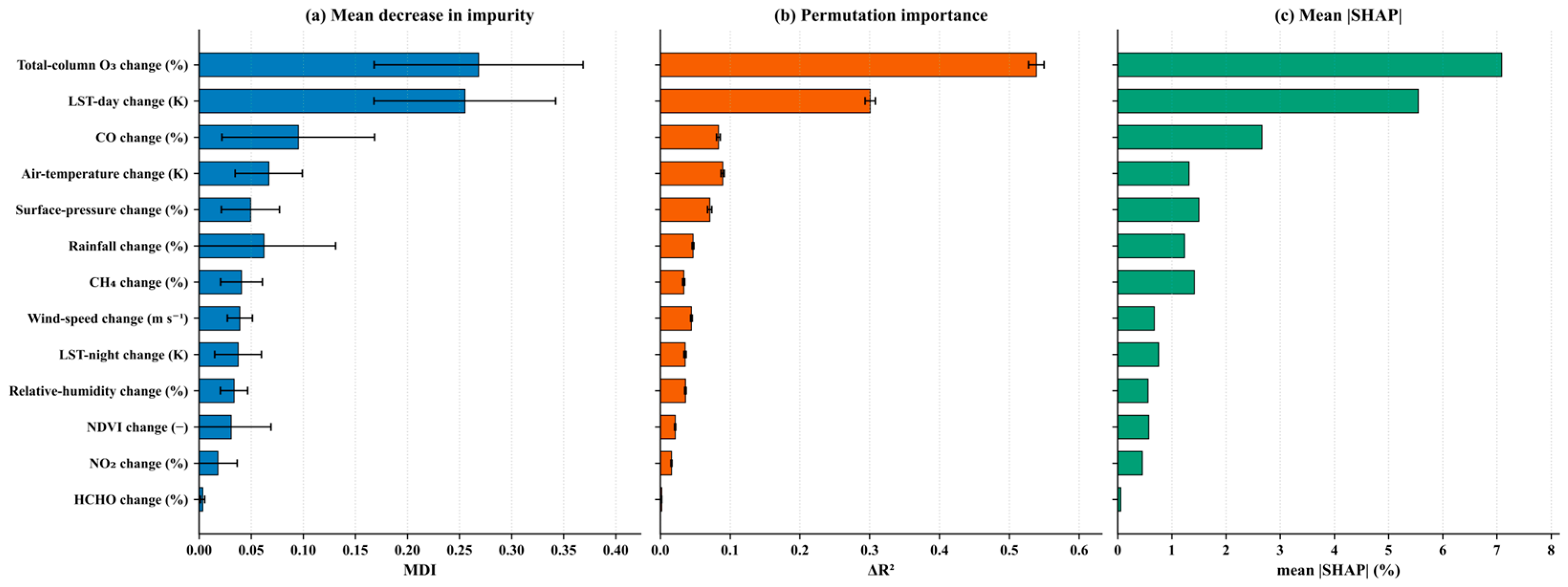
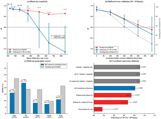
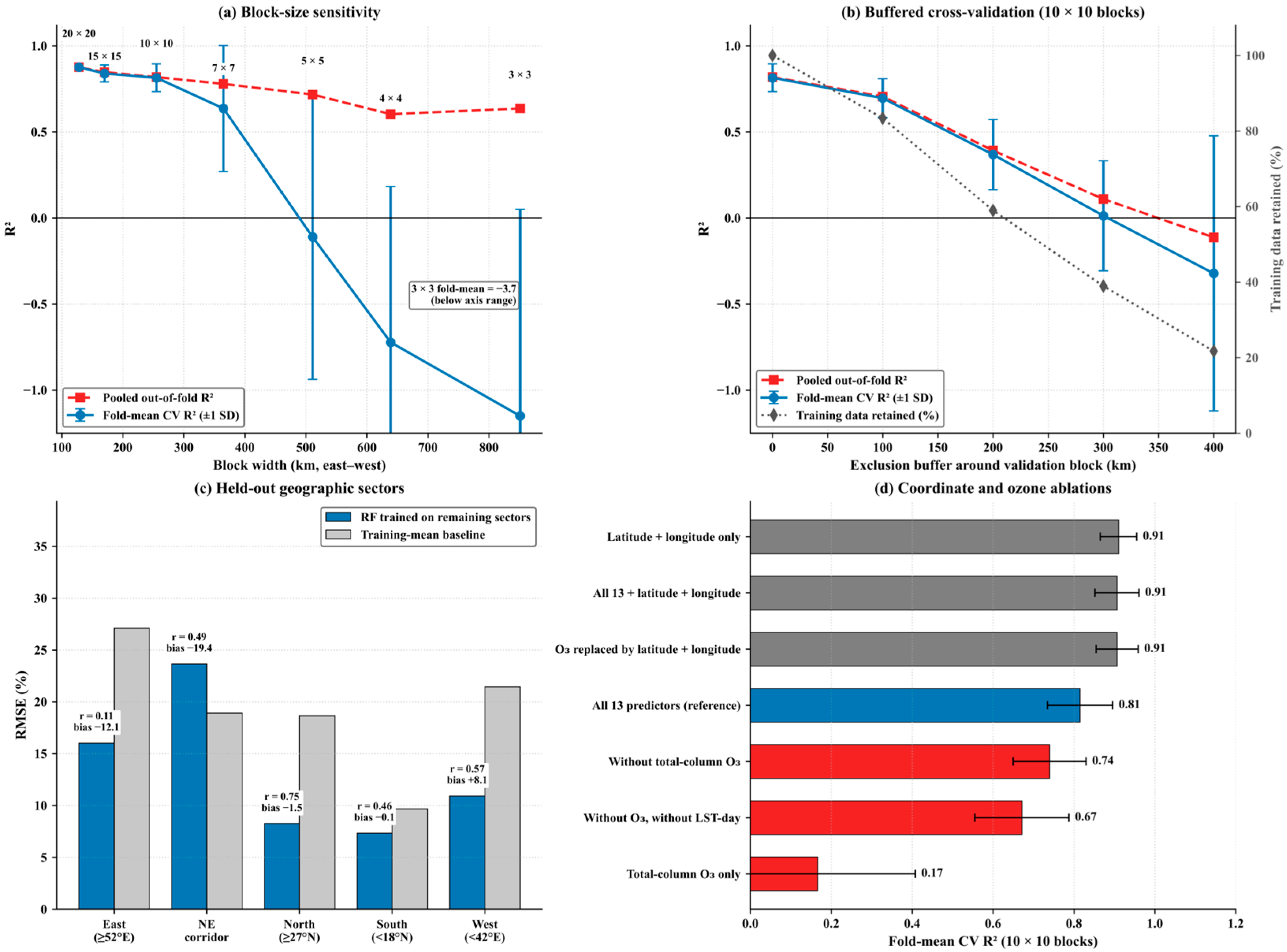

Disclaimer/Publisher’s Note: The statements, opinions and data contained in all publications are solely those of the individual author(s) and contributor(s) and not of MDPI and/or the editor(s). MDPI and/or the editor(s) disclaim responsibility for any injury to people or property resulting from any ideas, methods, instructions or products referred to in the content. |
© 2026 by the authors. Licensee MDPI, Basel, Switzerland. This article is an open access article distributed under the terms and conditions of the Creative Commons Attribution (CC BY) license.