Estimation of Soil Water Content in Winter Wheat Field at Jointing Stage Using Multi-Source Features and Machine Learning

Abstract

Accurate and timely monitoring of soil water content (SWC) plays an essential supporting role in crop irrigation management and smart agricultural practice. Remote sensing technology provides rapid and convenient approaches to large-scale farmland SWC estimation or inversion. However, existing mechanistic modeling methods are limited by parameter localization and land surface heterogeneity, while machine learning data-driven methods lack quite good physical interpretability. To address deficiencies in single data-driven methods and single vegetation microwave scattering models, and explore the estimation effect of different feature variables in machine learning. This study proposes an innovative estimation model that integrates machine learning strategies and multi-source features, including spectral indices and features derived from the classic water cloud model (WCM). The novelty of the proposed model lies in balancing physical interpretability and data-driven accuracy, namely extracting relevant soil backscattering parameters through WCM, which are then used as input features in the machine learning. A combination of field-measured data and unmanned aerial vehicle (UAV) multi-source remote sensing data, including multispectral and synthetic aperture radar (SAR) data, was acquired synchronously at the jointing stage of winter wheat. Through extracting variables such as the SAR microwave backscattering coefficient and the optical vegetation index, and conducting feature screening and parameter sensitivity analysis, we optimized the input variable sets of models based on back-propagation (BP) neural network, support vector regression (SVR) and random forest (RF) algorithms. The study results showed that the established estimation model had excellent estimation performance, especially for the RF algorithm, with the highest R² of 0.855, lowest MAE of 0.0212 cm³/cm³, and lowest RMSE of 0.0253 cm³/cm³. It was also shown that different feature input schemes have obvious effects on SWC estimation performance. On the whole, RF had the best estimation accuracy, followed by SVR and then BPNN. This study demonstrated that models integrating multi-source remote sensing data and machine learning could enhance SWC estimation ability for winter wheat fields, and could also serve as a promising approach for SWC monitoring in winter wheat fields in the North China Plain.

1. Introduction

Soil water content (SWC) plays an essential and significant role in crop growth monitoring, agricultural food production, and agricultural disaster prediction [1]. Therefore, rapid and highly accurate monitoring of SWC is important and has significant application prospects. Traditional approaches for SWC monitoring essentially rely on manual sampling and drying methods or fixed-position instrument measuring methods [2]. Though these approaches can obtain highly accurate SWC values, they waste time and energy, and lack spatial application value on a large regional scale [3]. With the continuous progress of remote sensing theory and technology, the non-destructive and rapid observation of agricultural environmental indicators has gradually been achieved [4]. In remote sensing estimation of SWC, commonly used remote sensing data sources include active microwave, passive microwave, multispectral, thermal infrared, and visible light [5,6]. Furthermore, the remote sensing platforms mainly include satellites, low-altitude unmanned aerial vehicles (UAVs), and ground-based equipment. The synthetic aperture radar (SAR) microwave can penetrate cloud layers and plant canopies and has all-weather observation capabilities. Many scholars have constructed various empirical and semi-empirical physical models, such as the IEM model, the Oh model and the AIEM model, to characterize the correlation between the SAR microwave backscattering coefficient and bare-land SWC, thereby achieving effective estimation of SWC [7,8]. In addition, multispectral and visible light optical data can be used to build statistical relationships between surface reflectance or vegetation indices and SWC. For vegetation-covered land surface, the most common estimation methods include the water cloud model (WCM), Michigan microwave canopy scattering model (MIMICS) and empirical model [9,10]. Among them, the WCM is widely used for the inversion of SWC on vegetation-covered surfaces. With its characteristic of large-scale coverage, satellite remote sensing has become the most commonly used method for inverting SWC on a regional scale. Furthermore, some scholars have proposed multi-source satellite data synergistic estimation methods [10]. Ermias Teferi et al. [11] integrated ASCAT SWI and Pedotransfer Functions to achieve enhanced surface soil moisture map-making. Xinyu Gao et al. [12] fused Sentinel-1 SAR and Sentinel-2 multispectral images, combined with ground measurement data, and compared the classic water cloud model with six typical machine learning models. Based on this, they constructed a WC-RFM model that deeply couples a mechanistic model and machine learning.

However, due to its low spatial resolution and interference from atmospheric factors, satellite remote sensing has shortcomings in accurately describing fine-scale agricultural areas [13]. Microwave satellite data usually have a spatial resolution of about 20 m, while optical satellite data are greatly affected by atmospheric conditions and plant canopy [14]. Meanwhile, the satellite revisit cycle leads to temporal and spatial misalignment when urgent decisions for crop irrigation and disaster prevention are required.

To compensate for the disadvantages of satellite remote sensing, UAV remote sensing has emerged and been widely applied in various fields. UAV remote sensing has the characteristics of maneuverability, flexibility, and strong real-time performance, and can achieve centimeter-level spatial resolution images. In addition, the characteristics of low-altitude flight make UAV remote sensing less affected by cloud and fog interference. With the proposal and development of machine learning algorithms, data-driven models such as random forest (RF), support vector regression (SVR), deep learning, and neural networks have been introduced into remote sensing inversion to extract various feature variables from multi-source data to improve the accuracy of SWC inversion [15,16]. In recent years, based on physical and machine learning models, many researchers worldwide have used UAV remote sensing to carry out SWC estimation research. Daowei Wang et al. [17] developed a UAV-borne dual-mode microwave radar observation system and established a data processing framework for high-resolution soil moisture retrieval, demonstrating its excellent ability for SWC prediction. Seo MinGuk et al. [18] designed a soil moisture retrieval model combining UAV multispectral and infrared images and the CNN algorithm; the results showed that the proposed CNN-based model had an advantage for prediction performance because it maintained the spatial information of pixels.

Although some progress has been made in existing research, there remain some unclear issues. The models and methods for SWC inversion are mainly divided into two categories: mechanistic models and data-driven models. Mechanistic models such as the WCM correspond directly to physical properties, but are limited by parameter localization schemes and surface heterogeneity, making it difficult to ensure estimation accuracy and lacking universality in practical applications. However, while machine learning and other data-driven models can extract nonlinear relationships from large amounts of data, significantly improving inversion accuracy, they have poor interpretability and rely on the quality of training data. Therefore, integrating mechanistic and machine learning models to balance physical interpretability and data-driven accuracy has broad research potential. In addition, the existing WCM–machine learning approach to feature variable selection is relatively casual and not sufficiently rigorous [19], often relying on Pearson’s correlation analysis [12]. Furthermore, some emerging remote sensing data sources, such as miniature SAR devices carried by UAVs, have rarely been used in soil moisture estimation research.

Wheat is the main staple food crop in North China, and Henan Province is an important national grain production base. The jointing stage is the peak period of water demand and the critical period for young ear differentiation in winter wheat, with water consumption accounting for 30–35% of the entire growth period [20]. Water directly determines the rate of tillering and ear formation, as well as the number of grains per ear. Drought and water scarcity can cause floral degeneration and a decrease in grain number per ear. Meanwhile, excessive soil moisture can easily lead to excessive elongation, lodging, and worsening of sheath blight in the basal internodes. Therefore, conducting SWC monitoring during the jointing stage of winter wheat has important research value and practical significance.

Given the above issues, this study focused on the winter wheat field in Xun County of Henan Province, China. At the jointing stage of winter wheat, farmland field sampling and UAV multispectral and UAV SAR remote sensing observation experiments were conducted within the study area. The Boruta algorithm was used to select key soil backscattering parameters and vegetation indices. The WCM and three machine algorithms (BPNN, RF and SVR) were coupled to build an SWC inversion model with both physical interpretability and high accuracy. Then, we systematically evaluated its performance and generalization ability in key growth periods and typical farmland areas. The study objective was to provide a reference for accurate monitoring of agricultural water conditions in the North China Plain.

2. Materials and Methods

2.1. Study Area

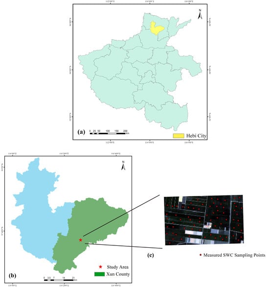
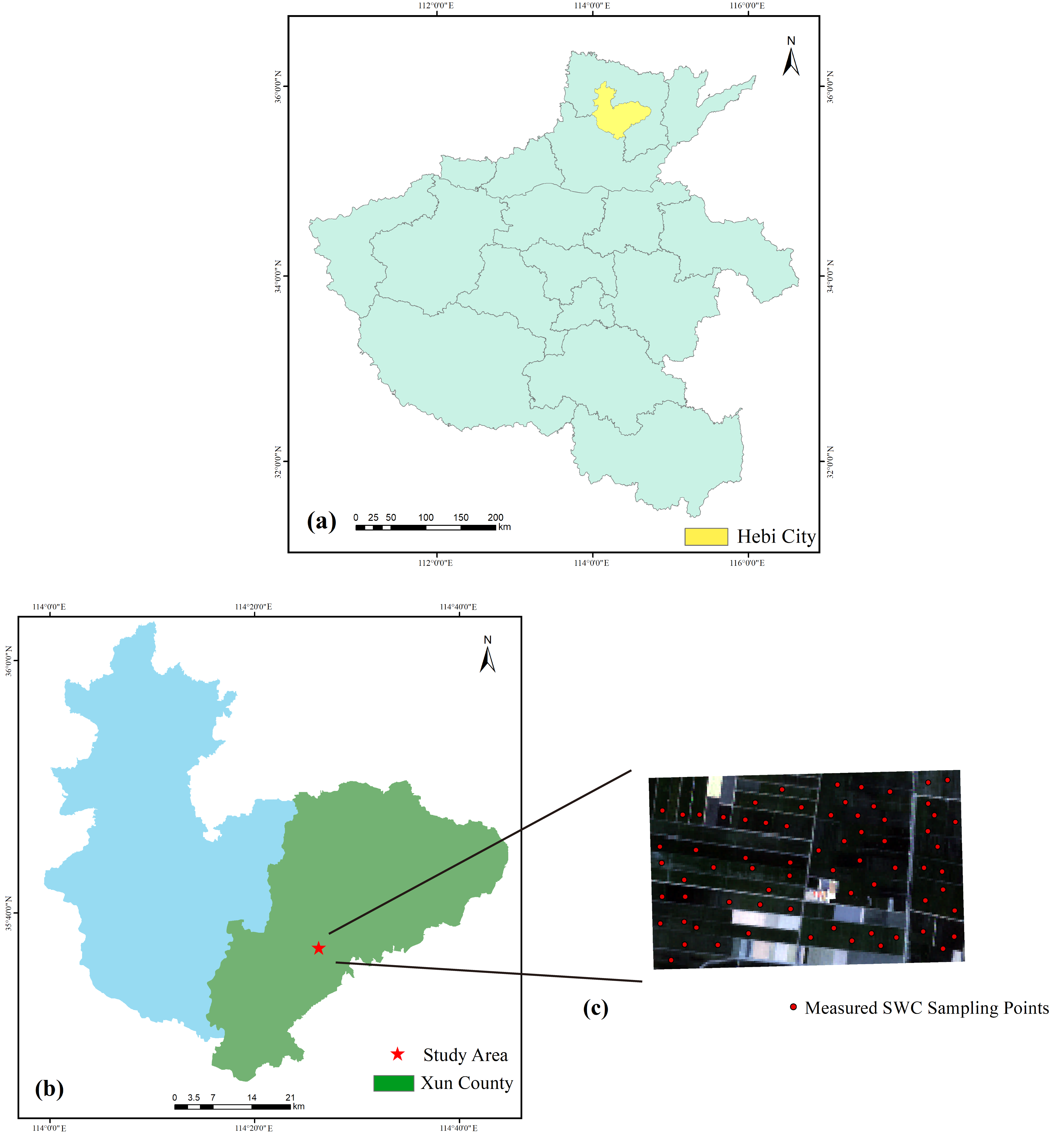
This study was carried out in Xun County, Hebi City, Henan Province, China. Located in an organized, flat region, the study area is a warm, temperate, semi-humid monsoon zone, with an area of 5.93 km². Winter wheat and summer maize are the most widely cultivated crops in this area. The location of the study area and measured SWC sampling points are illustrated in Figure 1.

Figure 1. Location of the study region and measured SWC sampling points.

2.2. Data Source and Processing

2.2.1. UAV SAR Data

SAR data were collected by a UAV equipped with an L-band SAR device independently produced by the Chinese Academy of Sciences. The SAR device works at a center frequency of 1.20 GHz. SAR data include VV and VH polarization modes, and the radar incidence angle is 78°.

The UAV SAR data processing workflow includes image mosaicking, system calibration, noise suppression, and geometric correction. The detailed preprocessing method can be found in reference [3]. The final mosaicked UAV SAR image achieved a spatial resolution of 0.60 m.

2.2.2. UAV Multispectral Data

On 31 March 2025, multispectral data were obtained using an M350 RTK UAV (DJI, Shenzhen, China) equipped with the RedEdge-Mx camera (MicaSense, Seattle, WA, USA), which covers five spectral bands: blue (475 nm), green (560 nm), red (668 nm), near-infrared (NIR, 842 nm), and red edge (717 nm). Multispectral data were collected from 11:00 to 14:00 Beijing Time on sunny days. Flights were conducted at a 70 m flight altitude and 80% frontal and side overlaps. After image mosaicking, radiometric calibration and geometric correction using Pix4D Mapper 4.5.6 software (Pix4D, Prilly, Switzerland), the final spatial resolution of the image was 0.20 m.

It should be pointed out that due to the limited UAV power endurance and lighting conditions, the coverage range of UAV multispectral images is smaller than that of UAV SAR images. Therefore, this study uses satellite multispectral data to fit and correct the study area’s UAV multispectral data. This study obtained Sentinel-2 satellite data from the transit study area on 1 April 2025. The specific Sentinel-2 image acquisition time is 11:05:19 Beijing Time on April 1, which was a sunny day. The time interval between UAV multispectral acquisition and Sentinel-2 acquisition is about 24 h. During this time interval, there was no rainfall or irrigation operation, and there was no significant change in SWC, so Sentinel-2 data can be used for correction of UAV multispectral data.

Due to the differences in spectral resolution between satellite data and UAV image data, it is necessary to correct the satellite spectral bands in order to achieve integration. With the range of a single pixel in the satellite image corresponding to each sampling point in the research area, the average reflectance of each band in the UAV image and the reflectance of a single pixel in the corresponding band are extracted. The ratio mean method was used to determine the correction coefficients for each band, and finally, the corrected spectral reflectance data covering the entire research area were obtained.

2.2.3. Field-Measured Data

Field-measured data collection was synchronized with UAV flight missions. No rainfall or irrigation events occurred during data collection. A total of 90 sampling points were selected in the experiments randomly and uniformly. The latitude and longitude of the sampling points were recorded using a high-precision GNSS RTK device (South Surveying & Mapping, Guangzhou, China), the measurement accuracy is in the centimeter level. Also, five ground control points (GCP) were selected within the research area, mainly obvious terrain points such as internal road intersections. RTK device with the same accuracy was used for measurement, serving as a common reference for geometric correction of UAV-SAR and UAV multispectral images, ensuring spatial uniformity of correction accuracy.

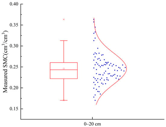
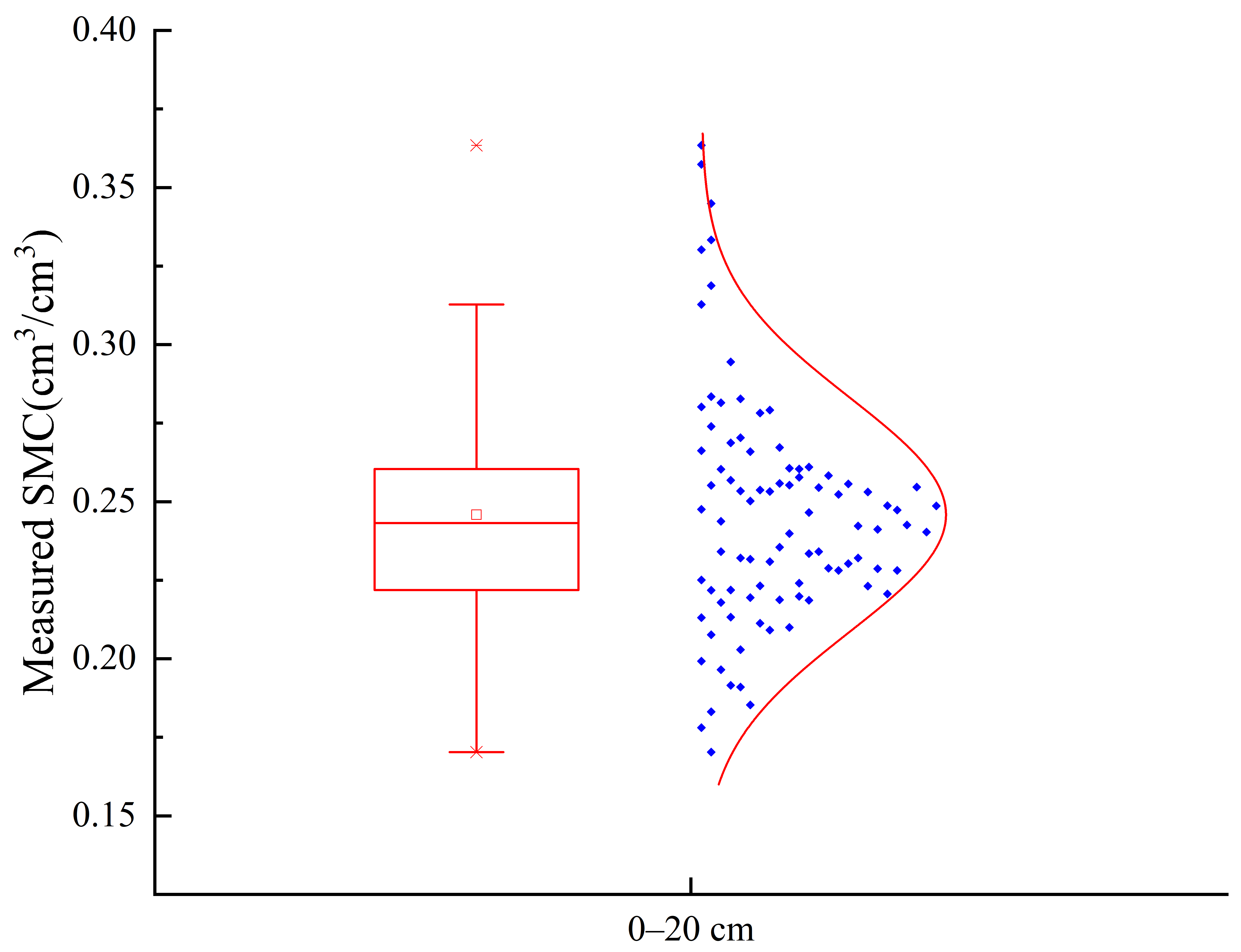
Field-measured SWC data were obtained in the 0–20 cm soil layer using the circular soil drill method. The gravimetric SWC was calculated using the oven-drying method at 105 °C until a stable weight was reached. The volumetric SWC was then calculated by multiplying the gravimetric SWC by the soil bulk density. After on-site measurement, the 0–20 cm layer soil bulk density value is 1.256 g/cm³. The measured SWC dataset was randomly separated into a training set and a testing set at a proportion of 80%:20%. Figure 2 shows the statistical results of the measured SWC data.

Figure 2. Statistics of measured SWC data.

2.3. Water Cloud Model

The water cloud model (WCM) was first created by Attema et al. [21] based on radiation transfer theory. The WCM can be expressed as

$${\sigma }_c^0\left(\theta \right) = {\sigma }_{\nu }^0\left(\theta \right) + {\gamma }^2\left(\theta \right) \times {\sigma }_s^0\left(\theta \right)$$

(1)

Among these,

$${\sigma }_{\nu }^0\left(\theta \right) = A \times m_{\nu }\cos \left(\theta \right)(1 - {\gamma }^2(\theta \left)\right)$$

(2)

γ²(θ) = exp(−2B × m_ν × sec(θ))

(3)

where ${\sigma }_{\mathrm{c}}^0\left(\theta \right)$ is the total backscattering coefficient of the vegetated area; ${\sigma }_{\mathsf{\nu }}^0\left(\theta \right)$ is the backscattering coefficient of the vegetation body; ${\sigma }_{\mathrm{s}}^0\left(\theta \right)$ is the soil backscattering coefficient of the underlying soil layer; γ²(θ) is the two-way attenuation factor; A and B are the empirical constants [4]; θ is the radar incidence angle; and m_ν is vegetation water content (VWC).

The m_ν is often calculated through vegetation indices such as NDVI and NDWI. Due to the lack of an empirical formula for localizing NDVI-VWC for winter wheat, this study used the typical relationship established by Jackson et al. [22] for maize and soybean crops. Many studies have also applied a constructed model for estimating m_ν of a certain crop directly to another crop [9,23]. The formula of this study is as follows:

m_v = 1.9134 × NDVI² − 0.3215 × NDVI

(4)

2.4. Machine Learning Algorithms

In this study, grid search and cross-validation were used to optimize the key hyperparameters of each algorithm, and the machine learning hyperparameter optimization was performed only on the training set data.

The BPNN algorithm is a multi-layer feedforward neural network trained using the back-propagation algorithm. This algorithm calculates the error between the actual output and the expected output, and propagates the error signal layer by layer to adjust the network parameters [24]. This study designed a three-layer architecture, namely the input layer, hidden layer, and output layer. The random seed of the BPNN is set to 2222, which is the “rng (2222)” in MATLAB. As for the parameter settings of the BPNN algorithm, key hyperparameters include a logistic sigmoid (logsig) activation function, a learning rate of 0.01, a maximum of 1000 training epochs, and a training error target value of 1 × 10⁻⁶.

RF is a statistical ensemble learning algorithm that can construct several decision trees from the training data, thus forming a “forest” of trained trees [25]. The RF regression model has strong adaptability to complicated datasets. In this study, the number of decision trees was set as 100, the minimum number of leaves was set as three, the maximum depth per tree was set as 70, and the minimum number of observations per leaf was set as three.

The SVR algorithm is an extension of the Support Vector Machine (SVM) algorithm for regression issues, mainly used for predicting continuous numerical values [26]. Its core goal is to find the optimal fitting hyperplane within a certain error range, combining nonlinear modeling capability and anti-overfitting properties. In this study, the kernel function was set as “RBF”, the penalty coefficient was set as 10, and the kernel function coefficient was set as “scale”.

In order to objectively evaluate the generalization ability of the algorithm and effectively prevent overfitting, 5-fold cross-validation was used to uniformly evaluate the three machine learning algorithms. The three machine learning algorithms were implemented in MATLAB R2022b (MathWorks, Inc., Natick, MA, USA). The general modeling procedure was divided into the training stage and the testing stage. After the training stage, the trained models were used in the testing stage.

2.5. Feature Variable Selection

Spectral indices are very useful in plant–soil water communication information and are suitable for estimating SWC. In addition, the SAR backscattering coefficient of the underlying soil layer (${\sigma }_{\mathrm{s}}^0\left(\theta \right)$) can reflect the physical state of and soil water. In order to compare the estimation ability of feature variables derived from different remote sensing data sources, this study selected nine spectral index variables and six SAR variables, as listed in Table 1.

Table 1. List of feature variables.

Feature Variable	Meaning/Formula
NDVI	${\displaystyle \frac{{\rho }_{\mathit{NIR}}-{\rho }_R}{{\rho }_{\mathit{NIR}}+{\rho }_R}}$
EVI	${\displaystyle \frac{2.5\times ({\rho }_{\mathit{NIR}}-{\rho }_R)}{{\rho }_{\mathit{NIR}}+6\times {\rho }_R-7.5\times {\rho }_B+1}}$
RVI	ρNIR/ρR
DVI	ρNIR − ρR
SAVI	${\displaystyle \frac{1.5\times ({\rho }_{\mathit{NIR}}-{\rho }_R)}{{\rho }_{\mathit{NIR}}+{\rho }_R+0.5}}$
TVI	60 × (ρNIR − ρG) − 100 × (ρR − ρG)
NDRE	${\displaystyle \frac{{\rho }_{\mathit{NIR}}-{\rho }_{\mathit{RE}}}{{\rho }_{\mathit{NIR}}+{\rho }_{\mathit{RE}}}}$
MCARI	[ρRE − ρR − 0.2 × (ρRE − ρG)]ρRE/ρR
OSAVI	${\displaystyle \frac{{\rho }_{\mathit{NIR}}-{\rho }_R}{{\rho }_{\mathit{NIR}}+{\rho }_R+0.16}}$
${\sigma }_{\mathrm{s},\mathrm{VV}}^0\left(\theta \right)$	VV polarization soil backscatter coefficient of underlying soil layer
${\sigma }_{\mathrm{s},\mathrm{VH}}^0\left(\theta \right)$	VH polarization radar total backscatter coefficient of underlying soil layer
${\sigma }_{\mathrm{s},\mathrm{VH}}^0\left(\theta \right)+{\sigma }_{\mathrm{s},\mathrm{VV}}^0\left(\theta \right)$	${\sigma }_{\mathrm{s},\mathrm{VH}}^0\left(\theta \right) \mathrm{plus} {\sigma }_{\mathrm{s},\mathrm{VV}}^0\left(\theta \right)$
${\sigma }_{\mathrm{s},\mathrm{VH}}^0\left(\theta \right)-{\sigma }_{\mathrm{s},\mathrm{VV}}^0\left(\theta \right)$	${\sigma }_{\mathrm{s},\mathrm{VH}}^0\left(\theta \right) \mathrm{minus} {\sigma }_{\mathrm{s},\mathrm{VV}}^0\left(\theta \right)$
${\sigma }_{\mathrm{s},\mathrm{VH}}^0\left(\theta \right)/{\sigma }_{\mathrm{s},\mathrm{VV}}^0\left(\theta \right)$	${\sigma }_{\mathrm{s},\mathrm{VH}}^0\left(\theta \right) \mathrm{divided\; by} {\sigma }_{\mathrm{s},\mathrm{VV}}^0\left(\theta \right)$
${\sigma }_{\mathrm{s},\mathrm{VH}}^0\left(\theta \right)\times {\sigma }_{\mathrm{s},\mathrm{VV}}^0\left(\theta \right)$	${\sigma }_{\mathrm{s},\mathrm{VH}}^0\left(\theta \right) \mathrm{multiplied\; by} {\sigma }_{\mathrm{s},\mathrm{VV}}^0\left(\theta \right)$

ρ_NIR, ρ_NIR, ρ_NIR, ρ_NIR and ρ_NIR refer to the reflectance of each spectral band, respectively.

3. Results

3.1. Feature Variable Screening by Boruta

In machine learning, it is important and necessary to screen a large number of feature variables to obtain variables that contain more information than noise. Feature selection algorithms are divided into filtering, packaging, and embedding methods. Filtering methods measure the importance of features based on different indicators. Packaging methods use feature subsets to train predictors, and then add or remove features based on selected criteria. Embedding methods obtain feature importance during model training. Due to the comprehensive understanding of the influencing factors of the dependent variable and efficient feature selection provided by the Boruta method, this study chose this method to select feature parameters, utilizing the Boruta package in R-4.6.0.

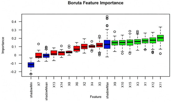
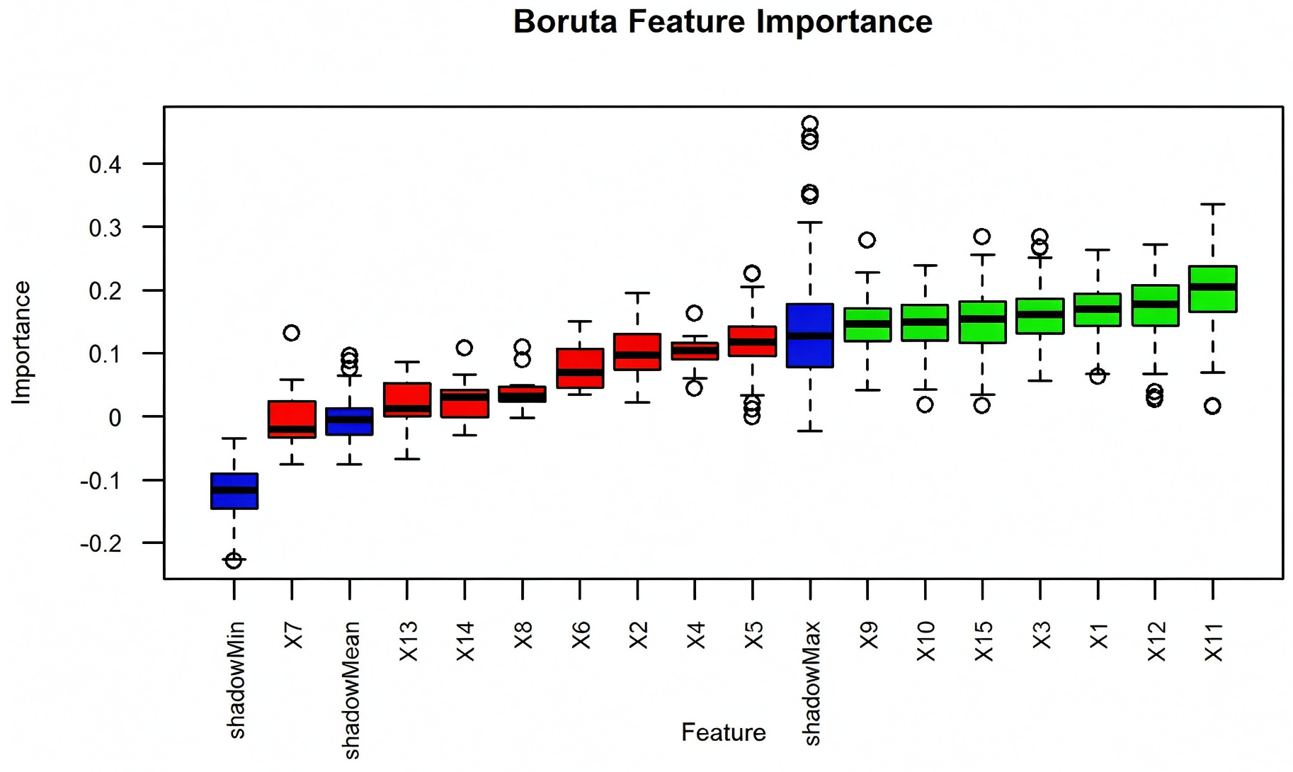
The Boruta method is a packaging method that creates shadow features and constructs a new feature matrix between the shadow feature set and the original feature set to compare the importance of real predictor variables with that of random shadow variables [27]. In this study, the Boruta feature selection was conducted only on the training set data. In order to facilitate Boruta feature screening mapping in R-4.6.0, we numbered all feature variables as shown in Table 2. Then, the Boruta method was used to screen 15 feature variables, the results of which are shown in Figure 3. The higher the importance score of a feature, the greater its impact on the prediction results. Therefore, this study selected seven feature variables that met the conditions for machine learning model construction, namely ${\sigma }_{\mathrm{s},\mathrm{VH}}^0\left(\theta \right)$, ${\sigma }_{\mathrm{s},\mathrm{VH}}^0\left(\theta \right) + {\sigma }_{\mathrm{s},\mathrm{VV}}^0\left(\theta \right)$, NDVI, RVI, ${\sigma }_{\mathrm{s},\mathrm{VH}}^0\left(\theta \right) \times {\sigma }_{\mathrm{s},\mathrm{VV}}^0\left(\theta \right)$, ${\sigma }_{\mathrm{s},\mathrm{VV}}^0\left(\theta \right)$, and OSAVI.

Table 2. Symbol names.

Symbol Name	Feature Variable
X1	NDVI
X2	EVI
X3	RVI
X4	DVI
X5	SAVI
X6	TVI
X7	NDRE
X8	MCARI
X9	OSAVI
X10	${\sigma }_{\mathrm{s},\mathrm{VV}}^0\left(\theta \right)$
X11	${\sigma }_{\mathrm{s},\mathrm{VH}}^0\left(\theta \right)$
X12	${\sigma }_{\mathrm{s},\mathrm{VH}}^0\left(\theta \right) + {\sigma }_{\mathrm{s},\mathrm{VV}}^0\left(\theta \right)$
X13	${\sigma }_{\mathrm{s},\mathrm{VH}}^0\left(\theta \right) - {\sigma }_{\mathrm{s},\mathrm{VV}}^0\left(\theta \right)$
X14	${\sigma }_{\mathrm{s},\mathrm{VH}}^0\left(\theta \right)/{\sigma }_{\mathrm{s},\mathrm{VV}}^0\left(\theta \right)$
X15	${\sigma }_{\mathrm{s},\mathrm{VH}}^0\left(\theta \right) \times {\sigma }_{\mathrm{s},\mathrm{VV}}^0\left(\theta \right)$

Figure 3. The results of Boruta feature screening.

The measured SWC dataset and corresponding features were randomly and uniformly separated into a training set and a testing set at a proportion of 80%:20%. The three feature variable input schemes shown in Table 3 were applied in SWC estimation models built using machine learning algorithms.

Table 3. Feature variable input schemes for machine learning algorithms.

Input Scheme	Input Variable
SAR-Variable	${\sigma }_{\mathrm{s},\mathrm{VH}}^0\left(\theta \right)$, ${\sigma }_{\mathrm{s},\mathrm{VH}}^0\left(\theta \right) + {\sigma }_{\mathrm{s},\mathrm{VV}}^0\left(\theta \right)$, ${\sigma }_{\mathrm{s},\mathrm{VV}}^0\left(\theta \right) \times {\sigma }_{\mathrm{s},\mathrm{VH}}^0\left(\theta \right)$, ${\sigma }_{\mathrm{s},\mathrm{VV}}^0\left(\theta \right)$
Spectral-Index Variable	NDVI, RVI, OSAVI
All-Variable	All variable above selected by Boruta

3.2. SWC Estimation Results Using Machine Learning Algorithms

3.2.1. SWC Estimation Results Using BPNN

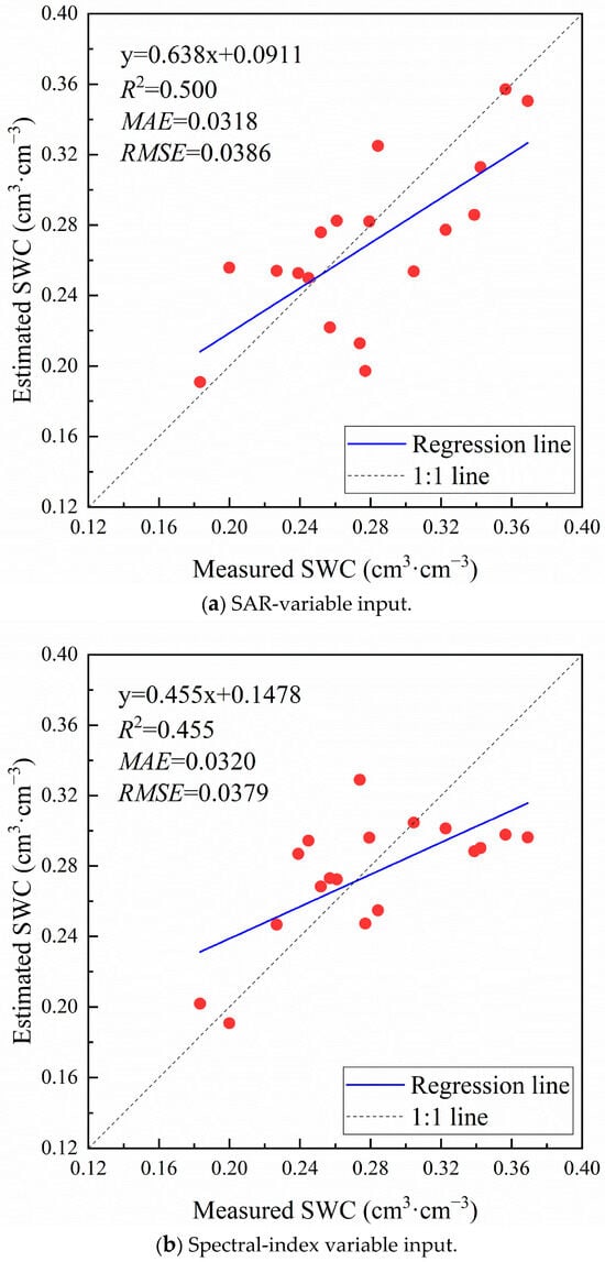
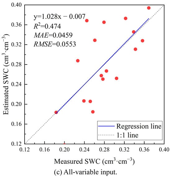
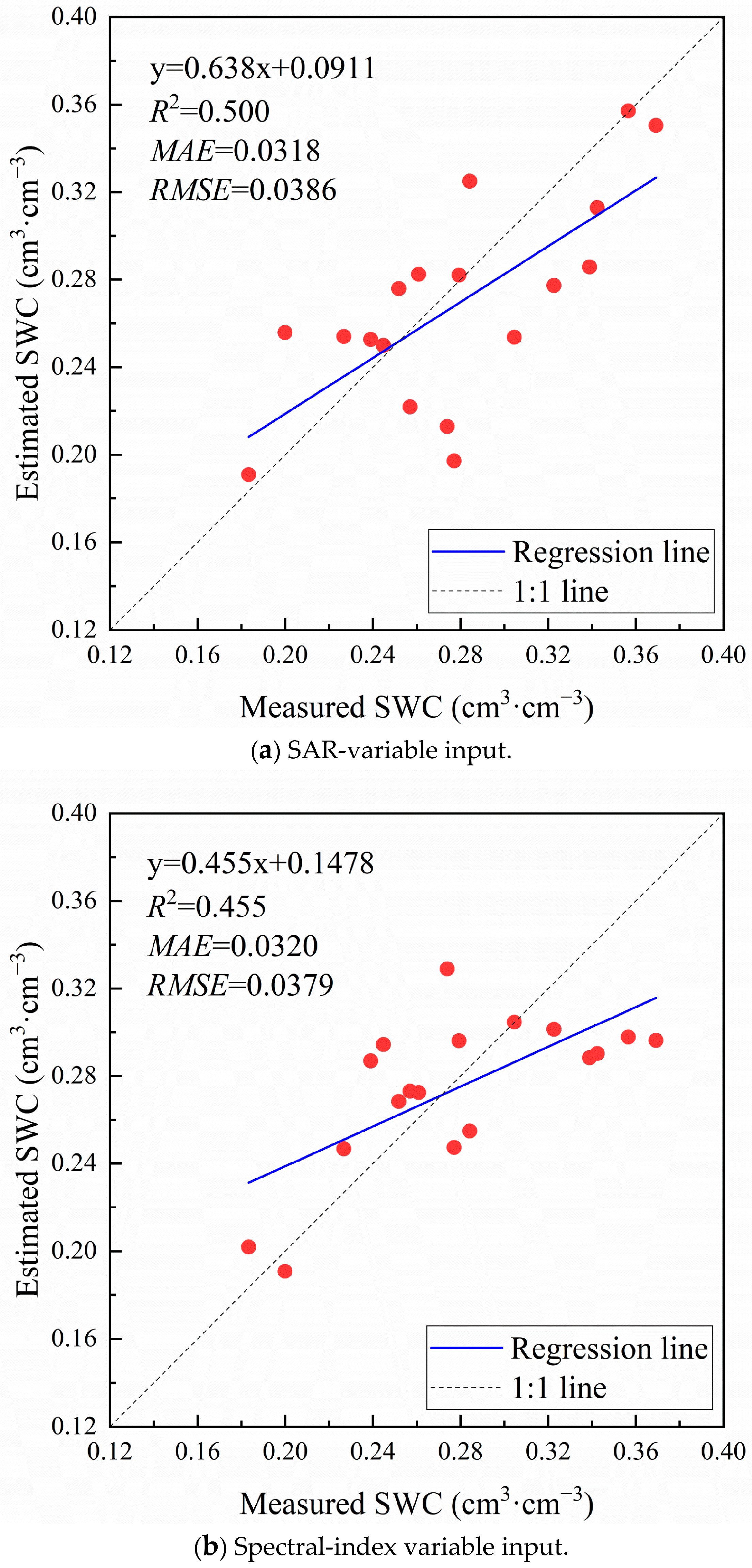
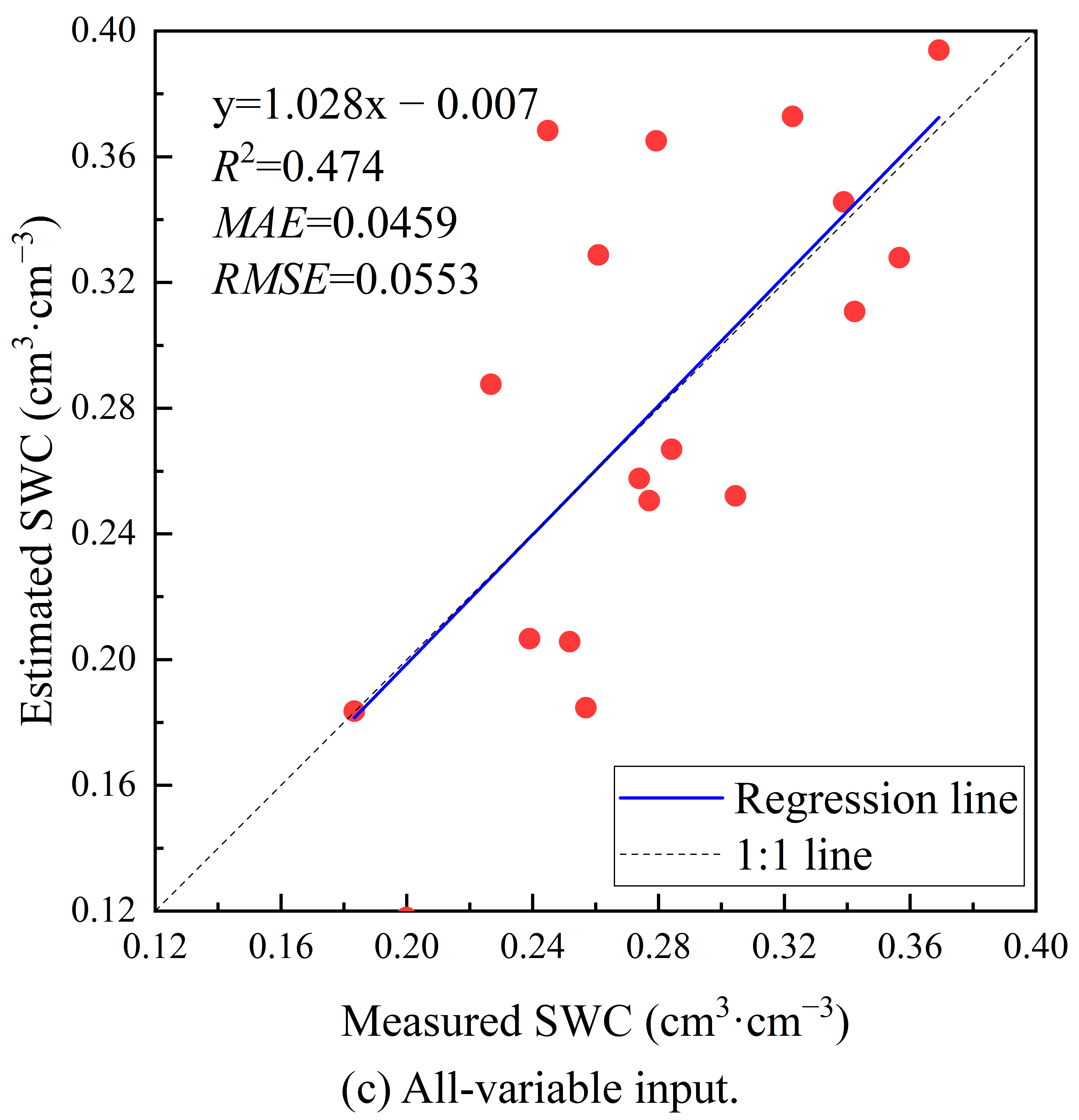
The BPNN-based estimation models were trained and then used on the testing set to evaluate performance and accuracy. The linear relationship between predicted SWC and measured SWC under different feature variable input schemes for the BPNN algorithm is illustrated in Figure 4.

Figure 4. SWC estimation performance using BPNN with different feature variable inputs.

The overall estimation accuracy using the BPNN algorithm was not high for these feature input schemes. As shown in Figure 4, the machine learning model with the SAR-variable input scheme reached relatively high prediction performance, with an R² of 0.500 and MAE and RMSE values of 0.0318 cm³/cm³ and 0.0386 cm³/cm³. The BPNN model using the spectral-index variable input scheme performed poorly, with an R² of 0.455. In contrast, the model based on the all-variable input scheme also showed relatively poor performance, with an R² of 0.474, an MAE of 0.0459 cm³/cm³, and an RMSE of 0.0553 cm³/cm³. From Figure 4a,b, it can be seen that the estimated SWC is higher than the measured SWC in low-value areas, and the estimated SWC is lower than the measured SWC in high-value areas. The scatter distribution is also more discrete. In Figure 4c, it can be seen that there are more scatter points below the 1:1 line, meaning that most of the estimated SWC is lower than measured SWC.

Overall, the BPNN algorithm integrated with various feature variable input schemes demonstrated weak estimation ability for SWC. In addition, it was demonstrated that the prediction ability of the BPNN algorithm may be affected by machine learning parameter settings and environmental conditions.

3.2.2. SWC Estimation Results Using RF

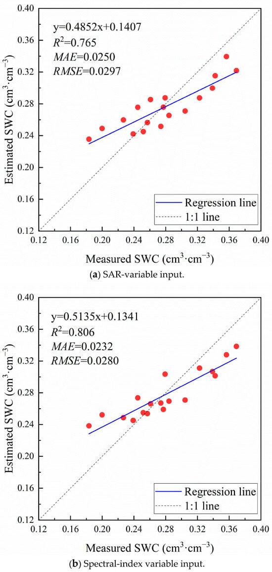
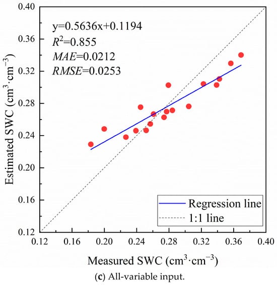
Similarly to the procedure conducted using the BPNN algorithm, training set data were applied to build the RF regression algorithm and create the SWC estimation model. The constructed estimation model was subsequently applied to the training set to acquire estimated SWC values.

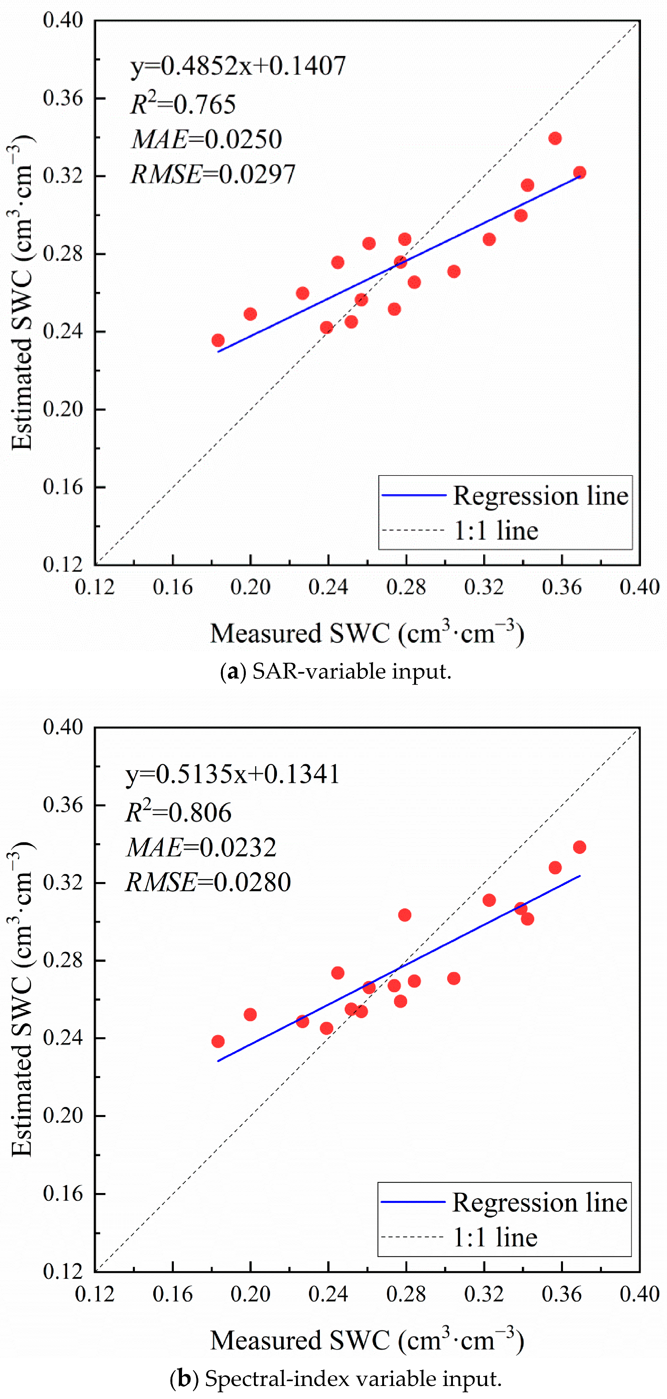
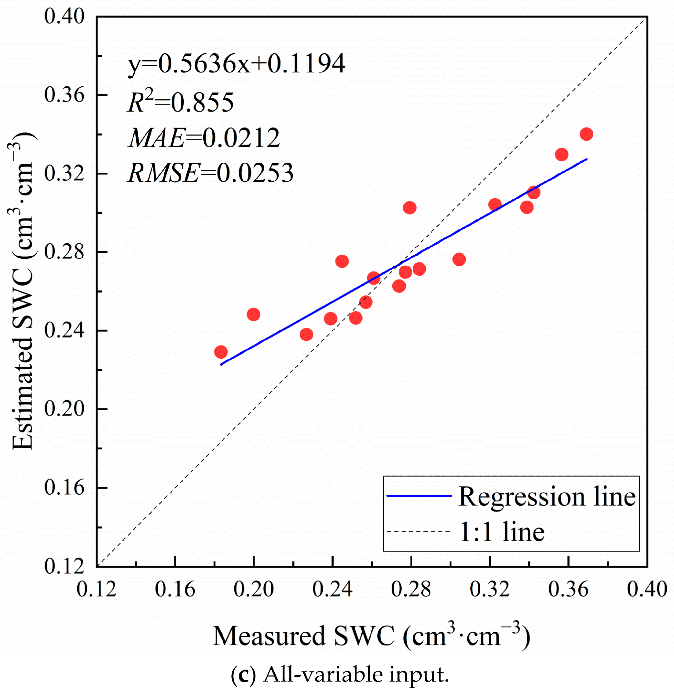
Figure 5 shows the consistency between the estimated and measured SWC values for three input schemes using the RF algorithm. For winter wheat at the jointing stage, it was discovered that the estimation model utilizing the all-variable input scheme achieved the best prediction effect, with an R² of 0.855, an MAE of 0.0212 cm³/cm³, and an RMSE of 0.0253 cm³/cm³. Meanwhile, the RF algorithm integrating the SAR-variable and spectral-index variable input schemes demonstrated fairly good performance, with an R² larger than 0.750 and MAE and RMSE values of less than 0.0250 cm³/cm³ and 0.0300 cm³/cm³, respectively.

Figure 5. SWC estimation performance using RF with different feature variable inputs.

From Figure 5, it can be seen that for the three input schemes of feature variables, the estimated SWC and measured SWC are closely distributed along the 1:1 line, and there is a clear phenomenon of “low value overestimation, high value underestimation”, but the overall deviation is small. Overall, the RF algorithm with these feature variable inputs achieved relatively excellent prediction results.

3.2.3. SWC Estimation Results Using SVR

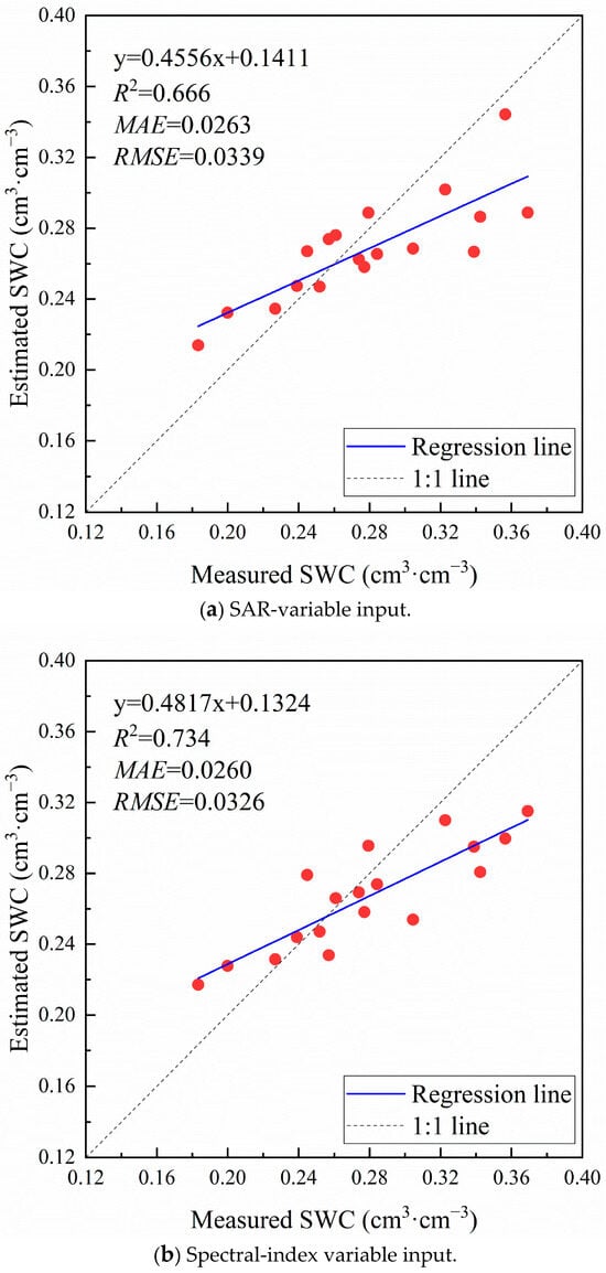
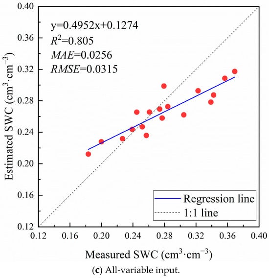
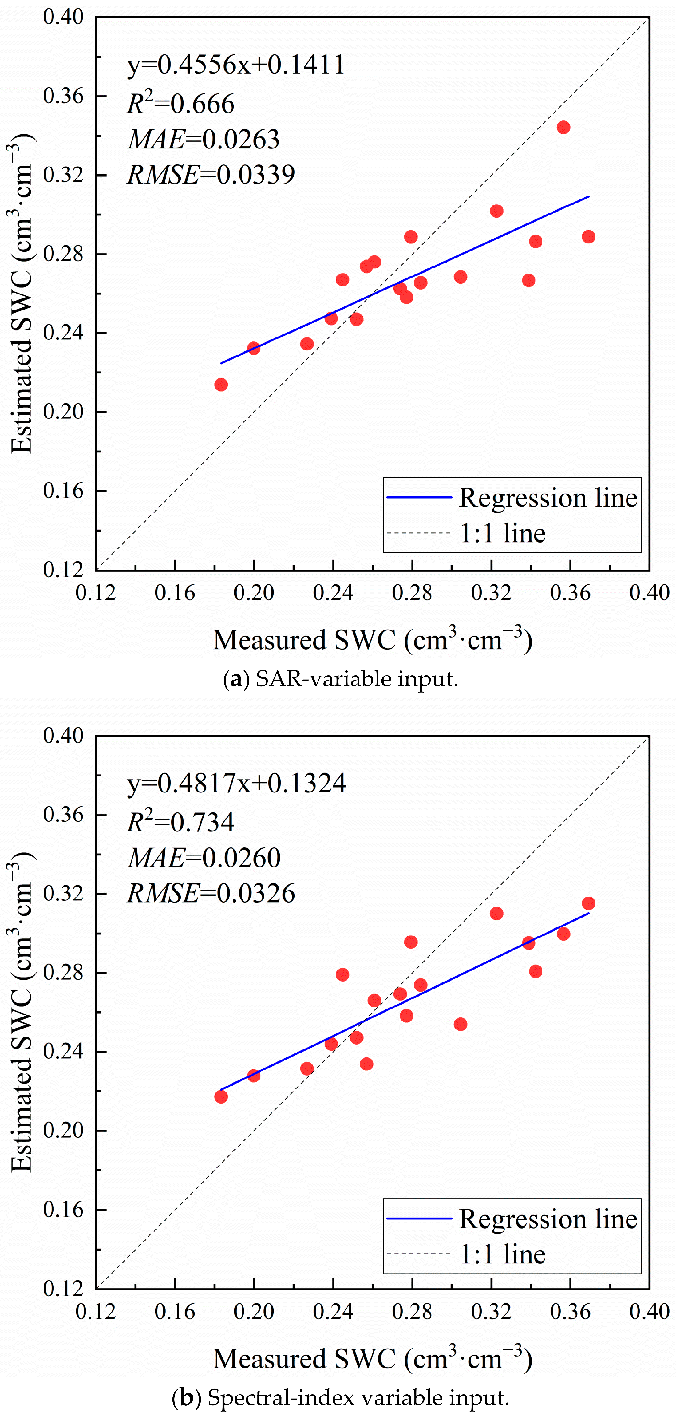
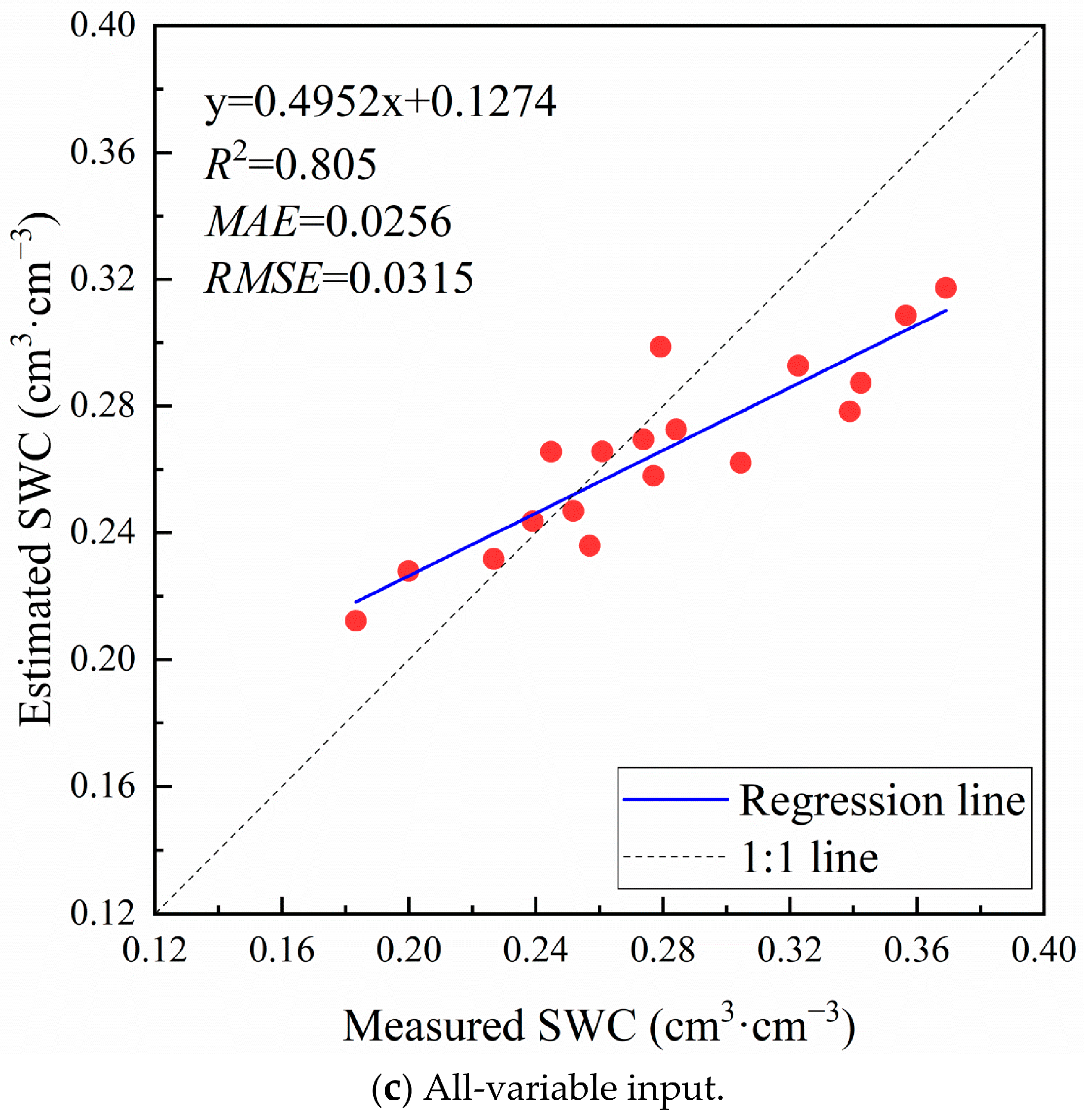
The SVR-based SWC estimation models were constructed and then applied to the testing set to evaluate performance and accuracy. The linear relationship between estimated and measured SWC under different feature variable inputs using the SVR algorithm is illustrated in Figure 6.

Figure 6. SWC estimation performance using SVR with different feature variable inputs.

It is shown that the overall estimation accuracy with SVR is relatively high, with an R² above 0.650 and MAE and RMSE values of less than 0.0300 cm³/cm³ and 0.0350 cm³/cm³, respectively. As shown in Figure 4, the SVR model with the SAR-variable input scheme reached relatively good prediction performance, with an R² of 0.666 and MAE and RMSE values of 0.0263 cm³/cm³ and 0.0339 cm³/cm³. The SVR models using the spectral-index variable input scheme performed better, with an R² of 0.734. In comparison, the machine learning model based on the all-variable input scheme exhibited the best prediction effect, with an R² of 0.805, an MAE of 0.0256 cm³/cm³, and an RMSE of 0.0315 cm³/cm³.

From Figure 6, it can be seen that for the three feature variable input schemes, there is also a clear phenomenon of “low value overestimation, high value underestimation”. Also, there are more scatter points below the 1:1 line, namely, the estimated SWC is lower than the measured SWC. However, compared to the RF algorithm, the overall deviation of SVR is relatively large. Overall, the SVR algorithm integrated with various feature variable input schemes showed strong estimation ability for SWC.

3.3. Comprehensive Analysis of SWC Estimation Results

Table 4 presents the accuracy evaluation of SWC estimation using three machine learning strategies under three feature input schemes; the p value is the overall significance F-test (ANOVA) result of univariate linear regression. Amongst these estimation results of nine combinations of algorithms and variable input schemes, the RF algorithm integrating the all-variable input achieved the best performance, with an R² of 0.855, an MAE of 0.0212 cm³/cm³, and an RMSE of 0.0253 cm³/cm³. In comparison, the worst result was obtained for the BPNN algorithm using the spectral-index variable input and all-variable input schemes, with an R² lower than 0.500 and MAE and RMSE values higher than 0.0300 cm³/cm³.

Table 4. Evaluation of SWC estimation accuracy using various machine learning algorithms and feature input schemes.

Input Schemes	Algorithm	R2	MAE (cm3/cm3)	RMSE (cm3/cm3)	p Value
SAR-Variable	BPNN	0.500	0.0318	0.0386	<0.001
	RF	0.765	0.0250	0.0297	<0.0001
	SVR	0.666	0.0263	0.0339	<0.0001
Spectral-Index Variable	BPNN	0.455	0.0320	0.0379	<0.005
	RF	0.806	0.0232	0.0280	<0.0001
	SVR	0.734	0.0260	0.0326	<0.0001
All-Variable	BPNN	0.474	0.0459	0.0553	<0.005
	RF	0.855	0.0212	0.0253	<0.0001
	SVR	0.805	0.0256	0.0315	<0.0001

In terms of a comparative assessment among the three machine learning algorithms, the results show that the RF algorithm is consistently superior to the BPNN and SVR algorithms for each feature variable input scheme, demonstrating its ability to achieve better performance in SWC estimation in winter wheat at the jointing stage. Meanwhile, between the BPNN and SVR algorithms, SVR usually achieved more accurate estimated SWC values for each input. Overall, the RF algorithm outperformed the BPNN and SVR algorithms in both stability and estimation capability for SWC.

In addition, among the three feature variable input schemes, the all-variable input achieved practically the highest estimation results when using each machine learning algorithm, whereas algorithms incorporating the SAR-variable input scheme showed relatively worse performance.

4. Discussion

The microwave SAR backscattering coefficient, spectral vegetation index, and other variables covered by vegetation on the ground usually contain rich information on land features. These variables are closely and complexly related to soil moisture and can serve as indirect indicators of soil moisture. Therefore, optimizing the selection of feature variables and estimating soil moisture under different feature input and machine learning algorithm conditions can provide a reference for intelligent farmland irrigation management.

In this study, the estimation results of various combinations of machine learning algorithms and feature input schemes showed that in most cases, better estimation accuracy could be obtained, with an overall R² greater than 0.500, an MAE of less than 0.0300 cm³/cm³, and an RMSE of less than 0.0350 cm³/cm³. Based on the quantitative evaluation in Table 4 and the visualization results in Figure 4, Figure 5 and Figure 6, the nine combinations of machine learning algorithms and feature variable input schemes showed clear and systematic performance differences in soil moisture remote sensing estimation. The estimation results of soil moisture indicate that the coupling application of machine learning and WCM effectively integrates physical laws and data patterns under medium to high vegetation coverage. They also reflect the powerful capability of data-driven methods in fitting complex nonlinear relationships.

When comparing the estimation results of the three machine learning algorithms for any specific variable input scheme, judging from evaluation indicators such as R², MAE, and RMSE, the order of estimation accuracy for the algorithms is RF > SVR > BPNN, with strong consistency. It is demonstrated that the best accuracy can be achieved by using RF for soil moisture prediction, which may be due to the complex nonlinear relationship between various characteristic variables and soil moisture, rather than a clear linear relationship. Meanwhile, compared to BPNN and SVR algorithms, RF has better representation ability and a better generalization level for nonlinear problems, making its effect on soil moisture inversion more significant. In contrast, the BPNN parameter settings used in this study performed the weakest results, with an R² mostly below 0.524 and an RMSE generally around 0.0400 cm³/cm³. This may be due to the sensitivity of BPNN models to noisy data, which reduces their generalization ability when dealing with high-dimensional data. This is consistent with the research findings of Que and Luo et al. [4,14].

In addition, regardless of which machine learning algorithm is used, there are differences in the inversion effects of the three different feature variable input schemes. Based on evaluation metrics such as R², MAE, and RMSE, for RF and SVR algorithms, the order of estimation accuracy for feature variable input schemes is ALL > VI > SAR, while for the BPNN algorithm, it is SAR > ALL > VI. In summary, inputting all feature variables yields better estimation results than inputting only SAR variables or spectral index variables, indicating that when all feature variables are used, more comprehensive soil moisture information can be gathered and better generalization performance can be achieved.

5. Conclusions

This study focuses on a typical winter wheat planting area in the North China Plain. In view of the difficulty of remote sensing inversion of soil moisture at the jointing stage under the conditions of medium and high vegetation coverage, we integrate UAV SAR, UAV multispectral, and ground-measured data, deeply couple a physical mechanism model (water cloud model) and a data-driven model (machine learning), and achieve efficient estimation and result analysis of soil moisture. The main conclusions are as follows:

(1)

Using the Boruta feature selection method, seven core features are ultimately selected from 15 candidate features. These features ensure a significant correlation with soil moisture and effectively control multicollinearity between features, laying a solid foundation for constructing robust soil moisture inversion models.

(2)

Among the three machine learning models, RF outperforms the other methods in terms of inversion accuracy and stability (R² = 0.855, RMSE = 0.0253 cm³/cm³, MAE = 0.0212 cm³/cm³), indicating that ensemble learning methods have significant advantages in modeling complex nonlinear relationships in jointing-stage farmland and are the most robust.

(3)

Among the three input schemes for feature variables, inputting almost all feature variables leads to the highest accuracy on the test set, reflecting a multi-dimensional and low-information-redundancy feature combination, with a strong ability to explain and characterize soil moisture changes.

There are still some shortcomings in this study, and future work could be carried out in the following areas:

(1)

This study has some limitations, such as the limited dataset, as well as the use of a VWC empirical formula originally developed for other crops. These factors will limit the generalizability of the research results.

(2)

When using the water cloud model to calculate soil backscattering, the influence of parameters such as surface roughness and plant height was not considered separately. In the future, these parameters can be obtained through ground-synchronous experiments to further localize and optimize the water cloud model, and research may explore coupling models with explicit features such as roughness and vegetation height.

(3)

The current model is mainly based on instantaneous remote sensing observations. In order to better serve agricultural production management, future efforts can be made to integrate time-series meteorological data, such as precipitation, temperature, evapotranspiration, and crop growth models, to construct a coupled model that can simulate the dynamic changes in soil moisture. This will enable a leap from state inversion to process simulation, ultimately providing more solid technical support for real-time monitoring and early warning of soil moisture in farmland.

References

- Chen, R.; Li, P.; Zhang, W.; Wang, H.; Wu, H.; Xu, X.; Zhang, L.; Wang, J. Simulation of soil water and nitrogen transport under drip fertigation using a dynamic infiltration boundary in HYDRUS. J. Hydrol. 2026, 678, 136089. [Google Scholar] [CrossRef] [Scilit]
- Esmaeilisarteshnizi, R.; Magagi, R.; Foucher, S.; Berg, A.; Colliander, A. Forest Soil Moisture Monitoring Using L-Band Passive Microwave and Machine Learning. Remote Sens. 2026, 18, 1970. [Google Scholar] [CrossRef] [Scilit]
- Lei, T.; Xiao, C.; Ce, W.; You, H. Fiber optic and TDR collaborative monitoring of spatiotemporal variation of soil moisture in citrus orchards. J. Irrig. Drain. Mach. Eng. 2026, 44, 531–540. [Google Scholar] [CrossRef]
- Que, Y.; Wu, D.; Jiang, M.; Deng, J.; Liu, C.; Wu, S.; Li, F.; Li, Y. Retrieving Soil Water Content in Winter Wheat Fields Using UAV-Based Multi-Source Remote Sensing and Machine Learning. Agronomy 2026, 16, 717. [Google Scholar] [CrossRef] [Scilit]
- Zhao, T.; Hu, L.; Shi, J.; Lü, H.; Li, S.; Fan, D.; Wang, P.; Geng, D.; Kang, C.S.; Zhang, Z. Soil moisture retrievals using l-band radiometry from variable angular ground-based and airborne observations. Remote Sens. Environ. 2020, 248, 111958. [Google Scholar] [CrossRef] [Scilit]
- Cheng, M.; Jiao, X.; Liu, Y.; Shao, M.; Yu, X.; Bai, Y.; Wang, Z.; Wang, S.; Tuohuti, N.; Liu, S.; et al. Estimation of soil moisture content under high maize canopy coverage from UAV multimodal data and machine learning. Agric. Water Manag. 2022, 264, 107530. [Google Scholar] [CrossRef] [Scilit]
- Yin, C.; Liu, Q.; Zhang, Y. Using the AIEM and Radarsat-2 SAR to Retrieve Bare Surface Soil Moisture. Water 2024, 16, 1617. [Google Scholar] [CrossRef] [Scilit]
- Shakya, A.K.; Ramola, A.; Vidyarthi, A. Integrated modelling of soil moisture by evaluating backscattering models Dubois, Oh and IoT sensor development for field moisture estimation. Model. Earth Syst. Environ. 2023, 9, 3381–3402. [Google Scholar] [CrossRef] [Scilit]
- Jing, H.; Chai, L.; Liu, S.; Chen, D.; Zhao, S.; Zhu, Z. Improve the accuracy of sar-based soil moisture retrieval by coupling bayesian inference and water cloud model. J. Hydrol. 2026, 666, 134826. [Google Scholar] [CrossRef] [Scilit]
- Jiang, J.; Hu, D.; Liu, Y.; Tang, X.; Li, J. Research on the inversion of surface soil moisture content in wheat fields based on MIMICS model. J. Wheat Crops 2015, 35, 707–713. [Google Scholar] [CrossRef]
- Teferi, E.; O’Donnell, G.; Kassawmar, T.; Mersha, B.D.; Ayele, G.T. Enhanced Soil Moisture Retrieval through Integrating Satellite Data with Pedotransfer Functions in a Complex Landscape of Ethiopia. Water 2023, 15, 3396. [Google Scholar] [CrossRef] [Scilit]
- Gao, X.; Meng, J.; Lin, Z.; He, R. Enhancing the surface soil moisture retrieval accuracy for winter wheat at thejointing stage by coupling the water cloud model with random forest. Trans. Chin. Soc. Agric. Eng. (Trans. CSAE) 2026, 42, 216–226. [Google Scholar] [CrossRef]
- Zhang, Z.; Wang, H.; Han, W.; Bian, J.; Chen, S.; Cui, T. Inversion of Soil Moisture Content Based on Multispectral Remote Sensing of UAVs. Trans. Chin. Soc. Agric. Mach. 2018, 49, 173–181. [Google Scholar] [CrossRef]
- Sun, H.; Wang, Y. Monitoring method for mining subsidence waterlogging based on multi-temporal SAR. J. China Coal Soc. 2026, 51, 1603–1623. [Google Scholar] [CrossRef]
- Zhang, Y.; Han, W.; Zhang, H.; Niu, X.; Shao, G. Evaluating soil moisture content under maize coverage using uav multimodal data by machine learning algorithms. J. Hydrol. 2023, 617, 129086. [Google Scholar] [CrossRef] [Scilit]
- Luo, Z.; Zhang, X.; Wang, Y.; Zhang, C.; Jiang, M.; Zhu, X. Surface Soil Moisture Retrieval over Winter Wheat Fields Based on Fused Multispectral and L-Band MiniSAR Data. Water 2025, 17, 3345. [Google Scholar] [CrossRef] [Scilit]
- Wang, D.; Cao, P.; Song, X.; Zhou, Y.; Han, W. A dual-mode UAV radar synergistic observation system and processing framework for high-resolution farmland imaging and soil moisture retrieval. Agric. Water Manag. 2026, 333, 110590. [Google Scholar] [CrossRef] [Scilit]
- Seo, M.-G.; Shin, H.-S.; Tsourdos, A. Soil Moisture Retrieval Model Design with Multispectral and Infrared Images from Unmanned Aerial Vehicles Using Convolutional Neural Network. Agronomy 2021, 11, 398. [Google Scholar] [CrossRef] [Scilit]
- Zhang, C.C.; Zhu, X.X.; Jiang, M.L.; Wang, R.; Hou, J. Soil moisture inversion of winter wheat based on uav minisar and multi-spectral remote sensing data. Water Sav. Irrig. 2025, 3, 105–112. [Google Scholar] [CrossRef]
- Zhu, Z.; Niu, X. Pays for the Hunan Army Analysis of Water Consumption and Water Consumption Patterns of Winter Wheat. Meteorology 1987, 13, 29–32. [Google Scholar]
- Attema, E.P.W.; Ulaby, F.T. Vegetation modeled as a water cloud. Radio Sci. 1978, 13, 357–364. [Google Scholar] [CrossRef] [Scilit]
- Jackson, T.J.; Vine, D.M.L.; Hsu, A.Y.; Oldak, A.; Starks, P.; Swift, C.; Isham, J.; Haken, M. Soil moisture mapping at regional scales using microwave radiometry: The Southern Great Plains Hydrology Experiment. IEEE Trans. Geosci. Remote Sens. 1999, 37, 2136–2151. [Google Scholar] [CrossRef] [Scilit]
- Cui, J. Remote Sensing Inversion of Soil Moisture Under Different Vegetation Conditions in Typical Grasslands: Based on Grazing Control Experiments. Ph.D. Thesis, Inner Mongolia University, Hohhot, China, 2023. [Google Scholar]
- Rumelhart, D.E.; Hinton, G.E.; Williams, R.J. Learning Representations by Back Propagating Errors. Nature 1986, 323, 533–536. [Google Scholar] [CrossRef] [Scilit]
- Breiman, L. Random forests. Mach. Learn. 2001, 45, 5–32. [Google Scholar] [CrossRef] [Scilit]
- Drucker, H.; Burges, C.J.C.; Kaufman, L.; Smola, A.; Vapnik, V. Support Vector Regression Machines. Adv. Neural Inf. Process. Syst. 1997, 28, 779–784. [Google Scholar]
- Kursa, M.B.; Rudnicki, W.R. Feature Selection with Boruta Package. J. Stat. Softw. 2010, 36, 1–13. [Google Scholar] [CrossRef] [Scilit]
Disclaimer/Publisher’s Note: The statements, opinions and data contained in all publications are solely those of the individual author(s) and contributor(s) and not of MDPI and/or the editor(s). MDPI and/or the editor(s) disclaim responsibility for any injury to people or property resulting from any ideas, methods, instructions or products referred to in the content. |
© 2026 by the authors. Licensee MDPI, Basel, Switzerland. This article is an open access article distributed under the terms and conditions of the Creative Commons Attribution (CC BY) license.