


Abstract
Laser weeding is a non-chemical, non-contact precision weeding method particularly suited for inter-row operations during the crop seedling stage. However, maintaining precise laser targeting on weed stems during dynamic field operation remains challenging. This task requires close coordination among perception, control, and actuation modules, while vehicle vibration from uneven terrain further degrades strike precision on the move. This paper presents a fully autonomous laser weeding robot for inter-row operation in cotton seedling fields, integrating weeding control, automatic mode switching, and autonomous navigation into a coordinated multi-process architecture. Vibration-induced strike deviation is mitigated by STCF-Net (Spatio-Temporal Cross-modal Fusion Network), a cross-modal prediction framework that fuses forward-looking depth maps with historical IMU signals to forecast vibration severity over a 3 s horizon. The prediction enables the control system to proactively adjust travel speed and weeding mode before encountering rough terrain, balancing precision and efficiency under dynamic field conditions. Field experiments validated weeding performance in static and dynamic scenarios and demonstrated that STCF-Net-guided predictive switching reduced operational time by 11.5% to 13.9% compared with a conservative baseline in two controlled experiments, with only a marginal reduction in weeding precision. This study reports the system-level design of a fully autonomous laser weeding robot and introduces feedforward vibration prediction to the laser weeding domain, providing a practical reference for integrating predictive algorithms into field-deployable weeding systems.
1. Introduction
Weeds are a major constraint on crop yields [1]. Traditional weeding methods each have their own drawbacks: manual weeding is labor-intensive, mechanical weeding disturbs the soil, and chemical weeding induces herbicide resistance and ecological risks [2]. Laser weeding uses focused high-energy beams to selectively destroy weed stem tissue, offering zero pesticide residue, no soil disturbance, and precise targeting of individual weeds. Laser weeding is therefore regarded as a promising approach to sustainable agriculture [3].
Laser weeding has advanced along three main lines: from handcrafted features to deep learning, from detection bounding boxes to keypoints, and from single modules to complete systems. Early systems relied on color segmentation and shape descriptors for weed identification, with limited field robustness [4]. The YOLO family rapidly became the mainstream approach due to its balance of detection speed and accuracy [5,6], and YOLO-based detection has been further integrated into complete in-field laser weeding systems [7]. As researchers recognized that detection bounding box centers do not correspond to weed stem positions, alternative strike-point representations were explored, such as the crop-region-removal and centroid targeting adopted by Xu et al. [8] in lily fields, while keypoint regression-based methods for direct stem localization gradually gained attention [9,10]. Building on these advances, recent work has begun to construct complete robotic systems: Zhao et al. [11] built a weeding robot for strawberry fields; Cao et al. [12] proposed a multi-tier differentiated weeding strategy; and Hu et al. [13] explored a mechanical-laser collaborative approach. Wei et al. [14] and Wang et al. [15] made advances in task planning and error compensation, respectively. Gao et al. [16] developed a weed detection scheme based on dual-model fusion together with a strategy for adaptively controlling laser power according to weed size.
Beyond perception, autonomous field operation also requires reliable navigation, and agricultural visual navigation is comparatively mature. Li et al. [17] identified image instability caused by rough terrain as a core bottleneck for machine vision in field visual weeding, while unstructured farmland and terrain variation remain persistent challenges for the autonomous navigation of field agricultural machinery [18]. Recent reviews frame the remaining open problems as robustness in unstructured terrain, real-time processing on embedded hardware, and the scarcity of field datasets [19], yet for row following, these problems are largely outweighed by the guidance accuracy already achieved in practice: the modular robotic system MARS kept 85% of a 537 m cotton-field path within 0.05 m [20], and LiDAR-based row detection reaches similar accuracy in simulation [21]. For laser weeding, however, path-tracking accuracy is not the binding constraint: the beam must strike individual weed stems from a moving platform, so terrain-induced vibration, rather than lateral error, dominates the error budget.
In recent years, researchers have increasingly recognized the constraints vibration imposes on laser weeding performance under dynamic conditions. This concern was substantiated quantitatively in weeding device validation, where the weeding rate decreased from 90.6% at 0.2 m/s to 81.5% at 0.6 m/s, a loss of 9.1 percentage points that the authors attribute to system vibration and image blur [22]. A similar speed-dependent degradation has been reported for intra-row mechanical weeding systems, where field trials showed the weeding accuracy dropping from 96.0% at 0.1 m/s to 81.8% at 0.5 m/s as the available response time decreased [23]. Lu et al. [3] noted that dynamic positioning accuracy is difficult to guarantee under complex terrain conditions and that the camera-to-actuator coordinate mapping suffers a performance gap between calibration and field environments. To cope with vibration effects, Wang et al. [15] expanded the laser scan coverage area to encompass the possible range of target deviation, while Andreasen et al. [24] suggested enlarging the laser spot diameter to improve the field hit rate. Gao et al. [16] reported that they fused IMU and wheel encoder data to estimate platform pose and corrected tilt-induced deviations in coordinate transformation in real time, although the underlying principle was not described in detail. Most other studies either operated in a stop-and-go mode for weeding [11,22,25,26], or specified that their machines only performed mobile weeding on flat ground [9].
From the above analysis, we observe that research on vibration-induced degradation of weeding precision during dynamic field operation remains limited: most existing platforms either operate in a stop-and-go mode or restrict mobile weeding to flat ground, while the strategies adopted to cope with vibration have been reactive rather than predictive. Some reported platforms are small-scale prototypes that may not reliably traverse real farmland and remain at the proof-of-concept stage. Taken together, these observations indicate that real-world weeding performance depends critically on how well the detection algorithm is matched to the machine’s system architecture and on the system’s ability to maintain precision under dynamic field conditions.
To address these challenges, this paper advances along two dimensions. At the system level, we present a fully autonomous laser weeding robot that integrates weeding control, automatic mode switching, and navigation into a unified multi-process architecture, enabling end-to-end field operation from perception to laser strike. At the algorithmic level, we propose STCF-Net (Spatio-Temporal Cross-modal Fusion Network), a cross-modal framework that fuses forward-looking depth maps with historical IMU signals to forecast vibration severity over a 3 s horizon. The overall objective of this study is therefore to determine whether precise laser weeding can be maintained without sacrificing operational efficiency during fully autonomous operation in actual farmland, where terrain-induced vibration continuously degrades strike accuracy. This objective is examined through three hypotheses: (i) integrating weeding control, automatic mode switching, and autonomous navigation into a coordinated multi-process architecture enables fully autonomous weeding in cotton fields; (ii) fusing forward-looking depth maps with historical IMU signals improves vibration-level prediction accuracy compared with modeling the IMU signals alone; (iii) a weeding strategy governed by the predicted vibration level reduces operation time relative to a conservative low-speed baseline while limiting the loss of weeding precision.
This study makes the following contributions:
- System-level design and field validation of a fully autonomous laser weeding robot. We integrated weeding control, automatic mode switching, and autonomous navigation into a hardware platform and validated the system end-to-end in field experiments, achieving a 97.18% static hit rate and approximately 4.8 h of continuous operation per full charge.
- STCF-Net, a cross-modal vibration prediction framework. It fuses forward-looking depth maps with historical IMU signals to forecast vibration severity 3 s ahead of terrain impact, introducing feedforward vibration handling to the laser weeding domain with 90.17% prediction accuracy.
- Predictive mode switching with quantitative field evaluation. The predicted vibration level directly governs travel speed and strike mode; in two controlled track comparisons, this predictive switching strategy reduced operation time by 11.5% to 13.9% compared with a conservative baseline in two controlled experiments, with only a marginal reduction in weeding precision.
The system is intended for autonomous inter-row weeding in cotton seedling fields, as an alternative to inter-row herbicide application and manual weeding. In deployment, the robot autonomously traverses the field along the crop rows fitted at startup, destroys seedling-stage weeds between rows by laser strikes, and is supervised by an operator via the remote controller. The approach targets the seedling stage of cotton, consistent with the agronomic practice of early weeding, and avoids both herbicide residue and soil disturbance in inter-row weed control.
The remainder of this paper is organized as follows. Section 2 describes the hardware platform and control algorithms, followed by the cross-modal vibration level prediction method (STCF-Net). Section 3 reports the field experimental results and their analysis. Section 4 discusses system limitations and directions for future work. Section 5 concludes the paper.
2. Systems and Methods
This section consists of three parts: first, the hardware platform of the robot; second, the control system architecture, which covers the three main modules of weeding control, automatic mode switching, and navigation control; and third, the design of the cross-modal vibration level prediction method.
2.1. Hardware Platform Design of the Laser Weeding Robot
The mechanical structure of the laser weeding robot is organized into three functional layers (Figure 1, Figure 2 and Figure 3):
Figure 1.
The laser weeding robot.
Figure 2.
Component identification of the laser weeding robot.
Figure 3.
Identification of the components inside the control cabinet of the laser weeding robot.
- Mobility platform layer: This layer consists of a wheeled chassis with front-wheel steering and rear-wheel drive, equipped with brakes and dampers. The track width, wheelbase, and ground clearance are matched to accommodate inter-row traversal and headland turning in cotton fields.
- Energy carrier layer: The laser serves as the weeding energy carrier. The high energy density of the laser beam combined with the precisely deflectable optical path of the galvanometer scanner enables non-contact, fixed-point strikes on inter-row weeds, avoiding mechanical disturbance to crops and soil while achieving high weeding efficiency.
- Perception and control layer: A hierarchical architecture based on an industrial computer and a slave controller integrates multimodal sensor data to coordinate the control of actuators, including the mobility platform, laser source, and galvanometer scanner.
The components and key parameters of each layer are listed in Table 1, Table 2 and Table 3. The whole machine is powered by the two lithium batteries listed in Table 2 (48 V, 120 Ah each, 11.52 kWh in total). In the endurance test, the robot performed normal weeding operation at the lowest speed level of 0.06 m/s in actual farmland, running continuously from full charge to battery depletion for approximately 4.8 h; during the test, the laser was active throughout the weeding segments along the field rows and was switched off only during headland turns. A demonstration of the integrated platform in operation is provided in Video S1 (Supplementary Materials).
Table 1.
Components and parameters of the mobility platform layer.
Table 2.
Components and parameters of the energy carrier layer.
Table 3.
Components and parameters of the perception and control layer.
2.2. Control System Architecture of the Laser Weeding Robot
2.2.1. Overall Control Architecture
The control system of the laser weeding robot adopts a multi-process architecture. Functionally, the system is divided into three main modules: weeding control, automatic mode switching and navigation control. Each module contains multiple processes running in parallel, exchanging data via shared memory. The overall system architecture is shown in Figure 4, and the main modules are as follows:
Figure 4.
Algorithm architecture diagram of the laser weeding robot.
- Weeding control module: Operates as a pipeline: the industrial camera captures field images, two YOLO models detect weed positions, thin-plate spline (TPS) transformation converts coordinates to the galvanometer coordinate system, and finally the system controls the galvanometer deflection and triggers the laser source to fire.
- Automatic mode switching module: Dynamically adjusts parameters such as travel speed and weeding mode (static/on-the-move strike) based on weed density and vibration level prediction results.
- Navigation control module: Generates a sequence of path segments consisting of straight weeding segments and turning segments based on the row direction and executes navigation segment by segment using the pure pursuit algorithm. Upon reaching the start and end points of each segment, the navigation module triggers the initial weeding mode corresponding to that segment.
2.2.2. Laser Weeding Control Module
The laser weeding control module implements an end-to-end pipeline from field image acquisition to laser strike, as shown in Figure 5.
Figure 5.
Laser weeding control module structure diagram.
Image Acquisition and Dataset Construction
Due to the lack of publicly available datasets suitable for the local cotton field and weed scenarios, we built a custom field image dataset. Images were acquired from April to December 2025 at a farmland site in Pudong, Shanghai, covering the complete growth cycle of cotton and weeds. The industrial camera mounted on the laser weeding robot captured vertically downward images of the weeding area. At a resolution of 2048 × 2048 and an imaging height of approximately 1.5 m, even small weeds were clearly visible.
The raw images underwent distortion correction before entering the subsequent pipeline. The checkerboard calibration method [27] was used to compute the camera intrinsic matrix and Brown-Conrady distortion coefficients, and each frame was corrected for distortion, yielding undistorted images for use by the weed detection model.
For each image, a custom tool was used to annotate the stem keypoint and the rectangular bounding box of the region containing each weed. The ISAT tool [28] was used for image segmentation annotation, labeling cotton leaves and dense weed regions, with Segment Anything v2 [29] assisting to improve annotation efficiency. During the keypoint annotation process, a keypoint detection model was trained on a small number of images and used for assisted annotation, reducing the workload. A total of 1136 images were annotated through the above process.
Keypoint annotation followed the unified criterion of “intended laser strike position,” because the essential goal of laser weeding is determining where to aim the laser, not distinguishing the root-stem structure. When the stem was visible, the stem base was annotated; when the stem was occluded by leaves, the center of the upper leaf was annotated to ensure at least leaf excision; for multi-stem weeds, the main stem was annotated; for long-stem weeds, the point closest to the ground was annotated to minimize deviations caused by inconsistent strike heights.
Dual-Model Training
Based on this dataset, two independent models were trained by transfer learning using the YOLOv8 framework [30] without modifying the network architecture. The built-in image augmentation scheme of the framework was used during training.
- Weed keypoint detection model (YOLOv8n-pose). Outputs weed bounding boxes and stem keypoint coordinates for rapidly locating candidate laser strike positions. Input image size: 2048 × 2048. In the laser weeding task, only precise localization of the weed stem is required, so keypoint accuracy was taken as the primary metric. The trained model achieved Pose mAP@0.5 = 0.853 with a Box mAP@0.5 = 0.554 on the test set.
- Instance segmentation model (YOLOv8n-seg). Outputs binary masks for cotton leaves and dense weeds. The cotton mask is used for subsequent coordinate filtering to prevent accidental crop damage, and the weed mask was used to determine whether to trigger area strike and to define the area strike region. Input image size: 720 × 720. The trained model achieved instance segmentation metrics on the test set of mAP@0.5 = 0.806.
After model training was complete, both models were quantized to FP16 precision using TensorRT (version 10.14.1) to improve inference speed.
Mask-Based Keypoints Filtering
Among the stem keypoints output by the weed keypoint detection model, some may be located near cotton plants. To prevent the laser from accidentally damaging crops, the cotton mask generated by the instance segmentation model is used, prior to coordinate mapping, to filter out keypoints within a certain distance of crop regions.
Since this coordinate filtering method is adopted for weed detection, a dual-model collaboration strategy of “broad annotation, post-filtering” is employed to balance detection sensitivity and model training difficulty. The keypoint model follows the principle of “annotate anything resembling a weed,” aiming to maximize recall without distinguishing specific weed species. Although we observed that a keypoint detection model trained in this manner has a certain probability of misidentifying seedling-stage crops as weeds, such false detections are subsequently filtered out by the cotton mask from the instance segmentation model. This dual-model collaboration simplifies the weed detection model’s task to “identify all plants that may be weeds” without requiring it to “distinguish between specific weed species and crops,” thereby reducing training difficulty and improving generalizability.
Camera-to-Galvanometer Coordinate Mapping Method
After identifying the pixel coordinates of weed stems, they must be converted to coordinates in the galvanometer coordinate system. The galvanometer deflects the laser beam via internal two-axis mirrors and maps the input galvanometer coordinates to corresponding strike points within a specified range on the ground. Since the actual cotton field ground surface is uneven—particularly the ridges formed by soil turned up during crop planting, which are higher than the reference plane—the depth value at each weed’s location, as detected by the depth camera, must also be taken into account.
We initially adopted a multi-stage coordinate transformation scheme. Starting from the measured relative positions of the camera and galvanometer and from the camera focal length parameters, we transformed the coordinates stepwise from the pixel coordinate system to the galvanometer coordinate system. However, because each parameter measurement introduced some error, the accumulation of errors across multiple transformation stages led to large overall system deviations. The errors mainly originated from the following two sources:
- Mounting position errors. It is difficult to mount the camera and galvanometer perfectly perpendicular to the ground, leading to perspective distortion. Moreover, their relative positions (horizontal and vertical distances) cannot precisely match the design parameters, resulting in inherent mounting deviations.
- Galvanometer coordinate system intrinsic errors. The galvanometer used exhibits non-uniform x- and y-axis scaling within its internal coordinate system, incomplete orthogonality between the axes, and pincushion distortion at the edges of the scan range. Although the galvanometer comes with coordinate system correction software, residual errors persist after correction.
To address these issues, this paper designs an end-to-end calibration approach that directly establishes a mapping from the pixel coordinate system to the galvanometer internal coordinate system.
Thin Plate Spline (TPS) interpolation [31] is adopted to establish this mapping. TPS can be viewed as an interpolation method that finds the smoothest surface with minimal bending energy under given control point constraints. Compared with pure polynomial fitting, TPS simultaneously captures the global affine transformation and local nonlinear deformations, making it suitable for this calibration problem. The analytic expression of TPS in its 2D form is the sum of a linear polynomial and radial basis function terms:
where the radial basis function , (xi,yi) are control point coordinates, with the additional constraints .
The 3D form of TPS is expressed as:
where the radial basis function is ϕ(r) = r, , (xi,yi) are control point coordinates, with the additional constraints . In the calibration described below, 3D coordinates (u,v,h) are taken as input, and a 3D TPS mapping function of the above form is separately established for each of the galvanometer coordinates x and y.
The specific calibration procedure is as follows. The galvanometer is controlled to project a 10 × 10 grid of galvanometer coordinates onto horizontally placed cardboard sheets at five different heights above the ground: 0, 6, 12, 18, and 24 cm. The industrial camera and depth camera capture images of the grids at all heights, and through manual annotation, the pixel coordinates (u,v) in the industrial camera image and the depth value (h) at that point in the depth camera are extracted for every grid intersection point. If a point’s depth is not detected by the depth camera, the average depth of surrounding pixels with valid depth values is used as a substitute. Thus, a total of 5 × 121 intersection points yield 3D coordinates (u,v,h), and the galvanometer coordinates (x,y) corresponding to each intersection point are known. The 3D TPS calibration method described above is then used to achieve a fitted mapping from 3D coordinates (u,v,h) to galvanometer coordinates (x,y). Then, the 2D TPS calibration method is used to establish the coordinate mapping from the industrial camera pixel coordinate (u,v) to the depth camera RGB image pixel coordinate (u′,v′).
After calibration is complete, for any weed stem pixel coordinate (u,v) in the industrial camera image that lies within the calibration range, the following two-stage process converts it to the coordinates (x,y) sent to the galvanometer. First, a 2D TPS transform is applied to obtain the pixel coordinates (u′,v′) in the depth camera image, and the depth value h at that pixel location is retrieved. Then, based on (u,v,h), a 3D TPS transform yields the corresponding galvanometer coordinates (x,y), which are the galvanometer coordinates for the weed stem position. Finally, these coordinates are sent to the galvanometer system, which automatically controls the laser source to fire and strike the specified position.
After completing the camera-to-galvanometer system calibration, an accuracy test was conducted. The vehicle was driven onto a farmland site with uneven terrain. n coordinates within the galvanometer’s range were arbitrarily selected in the image. These were converted via the calibration algorithm to galvanometer coordinates and sent to the galvanometer for single-point strike, producing burn marks on the ground. After all points were fired, the image was recaptured, and the pixel distance between the selected pixel coordinates and the actual burn-point coordinates in the image was measured and converted to physical distance, i.e., the positioning error. The calibration algorithm achieved an average error of 2.31 mm and a maximum error of 5.24 mm, meeting the weeding precision requirement.
Laser Strike Pattern
The calibrated target coordinates are fed into the laser strike control stage. The system provides two execution modes: single-point strike and area strike (Figure 6).
Figure 6.
(a) The red polyline shows the laser scan path for single-point strike under static and on-the-move conditions; green dots indicate weed stem positions. (b) The red line segments show the laser strike path for area strike.
Single-point strike: The weed stem coordinate is expanded into a zigzag scan path, with the start and end points of each segment alternating on opposite sides of a rectangular region, so that the laser spot traverses most of the rectangle’s area. The rectangle side length, number of scan lines, and the position of the stem within the rectangle are all adjustable via configuration files. Under static conditions, the scan region is a square of 21 × 21 px with the stem at the center. Under on-the-move conditions, the scan region is elongated along the travel direction into a rectangle; the length of the rectangle’s long side and its offset relative to the stem are adjusted according to the vehicle speed and control system latency, so that the actual strike pattern on the ground under motion is equivalent to that under static conditions.
Area strike: When weeds are dense and cover a large area, area strike is triggered to improve weeding efficiency. Area strike is triggered when the pixel area of the weed mask produced by the instance segmentation model exceeds a preset threshold Ath = 20%. Upon triggering, the weed mask is first compared with the cotton mask, and overlapping regions are removed to prevent the laser from entering crop areas. Subsequently, a set of parallel scan line segments with line spacing dline = 10 px is generated over the remaining weed mask. A smaller dline yields denser laser coverage; a lower spot traversal speed increases the dwell time and thus the energy delivered per unit area. In our configuration, the spot traversal speed along each scan line is set to 700 mm/s. The scan coordinates, after calibration transformation, are sent in batches to the galvanometer for execution.
2.2.3. Automatic Mode Switching Module
The automatic mode switching module dynamically adjusts travel speed and weeding mode based on the vehicle’s real-time state and terrain conditions, striking a balance between weeding precision and operational efficiency. The predicted vibration level, which is the core input to this module, is provided in real time by the cross-modal prediction network STCF-Net. This subsection first defines the two weeding modes, then describes the automatic switching strategy.
Static Strike and On-the-Move Strike
The system switches between static strike and on-the-move strike, which differ in the following execution logic.
Static strike (stop-and-go) is the default mode. Its work cycle is a continuous loop of “stop → standstill detection → image processing → coordinate transformation → strike → advance → stop.” After the vehicle stops, the standstill detection phase begins: the IMU mounted on the galvanometer base continuously reads triaxial vibration signals. When the vibration amplitude remains below a threshold Vstable = 0.015 m/s2 on all three axes (with the gravitational component removed from the z axis) for 2 s, the vehicle is determined to be fully stationary, and the next phase begins. During the strike phase, the detection results of both YOLO models are called in parallel: if the weed mask area is below a threshold Ath, single-point strike is used with the multi-frame aggregation strategy enabled (accumulating keypoint detection results from the past n = 5 frames and removing overlapping redundant keypoints via Non-Maximum Suppression, to mitigate occasional missed detections of small weeds). If the area exceeds Ath, area strike is used to sweep the weed region. The advantage of static strike is that it completely eliminates the effect of triaxial vibration during travel on laser strike points, yielding the highest precision; the cost is that stopping and standstill detection in each cycle consume additional time, reducing operational efficiency.
On-the-move strike is enabled when the ground is relatively flat and weed density is low, to improve operational efficiency. Area strike is not used in on-the-move strike, because speed fluctuations caused by uneven terrain and vibration would introduce large errors during prolonged, large-area continuous strikes. The work cycle is a continuous loop of “image processing → coordinate transformation → strike single weed → image processing.” In each loop iteration, only one weed is selected for striking. Based on the mounting positions of the galvanometer and the camera, a straight line is defined in the image, and the stem coordinate closest to this line is selected, so that the laser strikes the weed at an angle of approximately 70° relative to the ground. Finally, the coordinates are sent to the galvanometer, and upon receiving the “strike-complete” signal, the next round of detection and striking is immediately initiated. The galvanometer spot traversal speed can reach up to 2000 m/s, making the switching delay between different targets negligible.
On-the-move strike is divided into three speed levels: slow, medium, and fast. For each speed, coordinate delay compensation must be performed separately. During the interval from image acquisition to YOLO inference (processing time of 100–200 ms depending on weed density) and coordinate transformation to galvanometer strike (approximately 2–20 ms), the vehicle has already advanced a certain distance. The compensation method is to superimpose an offset Δs = Δt × k in the direction opposite to travel onto the original coordinates, where Δt is the time interval from image acquisition to the completion of coordinate processing, obtained by subtracting internal computer timestamps. The value of k is manually calibrated at each speed through field testing, k is 0.82, 1.19, and 1.50 at the slow, medium, and fast speed settings, respectively. For reverse travel, the offset is applied with the opposite sign; since the strike pipeline itself is independent of the travel direction, the per-weed strike performance in straight reverse travel is expected to be equivalent to that in forward travel.
Automatic Mode Switching
Field conditions vary dynamically with vehicle position: one segment may have flat ground and sparse weeds suitable for fast on-the-move strike, while the next may present furrows and dense weeds requiring speed reduction or switching to static strike for precision. The system switches modes automatically based on the following two metrics, evaluated continuously during operation.
- Weed density Dweed. The sliding-window average of the number of weed keypoint detections within the galvanometer strike range over the most recent m = 10 frames is computed. The weed density Dweed is compared against three preset thresholds T1 = 22, T2 = 15, T3 = 10 to preliminarily determine the strike mode, which is either static strike or on-the-move strike at three speed levels.
- Vibration level prediction Vpred. STCF-Net outputs in real time the predicted vibration severity level Vpred (low/medium/high) over the next 3 s. This network fuses the forward-looking depth map with historical IMU vibration signals and completes its assessment before the vehicle physically encounters the uneven road surface (see Section 2.3). The speed is then adjusted according to the speed level determined in the previous step and the predicted vibration level: when the predicted level Vpred was “high,” the speed is reduced by one level, down to a minimum of stop-and-go strike, to prevent precision loss during severe vibration. When Vpred is “medium,” the system maintains the current speed under the aggressive strategy or reduces speed by one level under the conservative strategy (user-configurable). When Vpred is “low,” the current speed is maintained. A minimum switching interval of 7 s is set to prevent the system from making consecutive switches while the vehicle was still in an unsettled state.
2.2.4. Navigation Control
Navigation control drives the robot along a predetermined route to traverse all field rows, triggering the weeding process upon reaching designated positions. The navigation module architecture is shown in Figure 7.
Figure 7.
Navigation control module structure diagram.
Hardware Interface
The navigation system relies on the Global Navigation Satellite System (GNSS) equipment (10 Hz positioning output) and the rear-wheel drive motors described in Section 2.1. The front-wheel steering motor introduces an engineering problem: the worm gear and rocker arm mechanism produce a nonlinear mapping between motor rotation and steering angle, with different mapping curves for left and right turns. These curves were separately fitted by quadratic interpolation from measured data and encapsulated into a unified steering interface. The minimum turning radius of the vehicle is 4.4 m.
Path Planning
Upon startup, the vehicle drives straight along a crop row for 5–10 m, collecting a GNSS trajectory from which the row direction vector is fitted by least squares. The task is then decomposed into an ordered sequence of weeding segments (straight travel with simultaneous weeding) and turning segments (no weeding), as shown in Figure 8. Each segment is decomposed into equally spaced waypoints and persisted to a file, enabling breakpoint resumption after work interruption. Subsequent segments chain from the endpoint of the previous one.
Figure 8.
Path planning schematic. Scheme 1 uses U-turn-based segment planning, with the machine always moving forward. Scheme 2 uses reverse-turn-based segment planning, with the machine moving forward in one adjacent straight segment and in reverse in the next.
Path Tracking Algorithm
The pure pursuit algorithm [32] was adopted for path tracking. This algorithm exhibits strong robustness to road undulations, GNSS positioning errors, control system latency, and actuator precision deviations in low-speed scenarios. The drawback of pure pursuit is that the tracking error significantly increases during high-speed turns. However, for cotton field weeding operations, turns occur only at headlands, and speed is limited to a low level, and no weeding is performed during turns, so the impact of this drawback is negligible (Figure 9).
Figure 9.
Schematic diagram of the pure pursuit algorithm.
The steering angle, computed from the Ackermann model, is given by:
where L is the vehicle wheelbase, ld is the straight-line distance from the vehicle’s current position to the look-ahead point, and α(t) is the angle between the vehicle heading and the line connecting the vehicle to the look-ahead point at time t.
The look-ahead point is determined using the cumulative distance method: The point on the path closest to the vehicle, Pnearest, is found. From Pnearest, the system advances along the path until the cumulative distance first reaches the preset look-ahead distance ld. The value of ld is set to 1.2 m for forward travel, 0.8 m for turning, and 1.6 m for reversing.
Manual Override
A remote controller process runs independently at the highest priority and can interrupt autonomous operation at any time to switch to manual control. The controller maintains an internal finite state machine toggling between stop-and-go strike, on-the-move strike, and autonomous navigation through button combinations.
2.3. Cross-Modal Vibration Level Prediction Algorithm
2.3.1. STCF-Net Architecture
During the dynamic operation of the laser weeding robot, the triaxial vibration generated as the vehicle travels on uneven farmland is the primary factor causing degradation in on-the-move weeding precision. Although a spring damping device is installed beneath the galvanometer scanner, it can only partially attenuate the vibration amplitude. For a machine subjected to prolonged severe vibration, precision optical components such as the galvanometer scanner may also undergo minute, irreversible displacements on their mounting base, forcing the system to recalibrate the parameters.
This study initially envisioned predicting the triaxial displacement of vehicle vibration point by point and superimposing a feedforward compensation amount during galvanometer strike to cancel the vibration-induced offset. However, experiments revealed that the unevenness of farmland surfaces behaves as a random signal, so the specific triaxial vibration displacement at a future moment cannot be reliably predicted. Further analysis showed that, although randomness makes pointwise displacement prediction infeasible, predicting the overall vibration severity over a future time window is viable, and the level information is sufficient to provide effective guidance for weeding strategy decisions.
This subsection proposes a cross-modal prediction method that fuses forward-looking depth maps with historical vibration signals. The core intuition is that depth maps provide spatial information about the road surface ahead, while historical vibration signals capture the vehicle’s temporal state. By fusing these two modalities in the spatio-temporal dimension, the vibration level can be assessed before the physical impact occurs, enabling proactive adjustment of the weeding mode. To implement this fusion, we propose the Spatio-Temporal Cross-modal Fusion Network (STCF-Net), whose core design philosophy is “vision-guided temporal early warning”: encoded historical vibration information serves as the query to attend to different regions in the forward-looking depth map, achieving feature fusion across the two modalities. STCF-Net consists of three modules: a temporal encoder, a spatially aware visual encoder, and a cross-modal cross-attention mechanism. The overall architecture is shown in Figure 10.
Figure 10.
Architecture diagram of STCF-Net.
Temporal Encoder
IMU vibration signals are typical non-stationary sequences containing high-frequency impulse components (sharp acceleration pulses generated when a wheel momentarily strikes a stone) and low-frequency undulation components (sustained vehicle body sway caused by continuously uneven road surfaces). Because these two types of components differ substantially in time scale, convolution kernels with a single receptive field cannot capture both simultaneously; a multi-scale architecture is therefore required. This module uses InceptionTime [33] as its backbone. By employing multiple 1D convolution kernels with different receptive fields in parallel within Inception modules, InceptionTime can automatically extract frequency features at different scales from the time series without requiring preprocessing such as Fourier or wavelet transforms on the input.
Standard InceptionTime uses global average pooling (GAP) at the final layer to compress the entire temporal dimension into a single vector. However, in this task, GAP averages all time steps with equal weight, so its output is diluted by long segments of stationary signals. We therefore replaced GAP with an attention pooling layer that enables the model to automatically identify the most discriminative impulse waveforms in the sequence and assign them high weights, thereby suppressing random noise and improving cross-modal alignment in the subsequent cross-attention.
Spatially Aware Visual Encoder
The design of this module is inspired by the ViT approach of partitioning images into patch sequences [34], with the goal of transforming the forward-looking depth map into a token sequence that preserves spatial topological relationships, for subsequent spatial localization by cross-attention. However, depth maps contain only single-channel distance information with low information density, and the amount of data in this task is limited. The convolutional inductive bias of CNNs is more efficient and easier to train in this scenario than the original attention layers used in ViT, while also reducing end-side inference overhead.
We adopted a CNN to perform hierarchical feature extraction on the input depth map D ∈ , progressively reducing spatial resolution while increasing channel depth, to obtain a feature map F ∈ RC×h×w. The feature map is then flattened along the spatial dimensions into a token sequence:
On the feature map after CNN downsampling, each token can be understood as the feature aggregation of a receptive field region in the original depth map, equivalent to dividing the road surface ahead of the vehicle into a grid along spatial dimensions, with each grid cell corresponding to one token. Following the ViT approach, 2D sinusoidal positional encoding is introduced for each spatial token, embedding the spatial position information of different regions into the token. In the depth map, the proximal rows correspond to the road surface immediately ahead of the vehicle, whereas the distal rows provide early-warning information; the positional encoding allows the model to exploit this cue to relate spatial position to the timing of the upcoming vibration.
Cross-Modal Cross-Attention
The forward-looking depth map and the historical vibration signal constitute two heterogeneous modalities, one spatial and one temporal, whose correspondence is difficult to capture by direct concatenation or element-wise addition. This module therefore employs a cross-attention mechanism [35] to model the interaction between the two modalities, enabling the network to learn which terrain feature gives rise to which vibration response.
Let the visual token sequence be Zimg ∈ RL×d, and the temporal encoder output be . The two modalities are projected into the same representation space:
where are learnable parameters. The attention scores are then computed, and the values are aggregated by weighted summation:
The attention mechanism enables the spatial features of the depth map and the temporal features of the vibration signals to interact at the representation level. Finally, the aligned features produced by the cross-modal cross-attention and the original vibration features (without cross-modal interaction) are processed through their respective branches and concatenated. The concatenated features are then passed through a fully connected layer and a softmax layer to produce the three-level vibration severity prediction.
2.3.2. Data Acquisition and Preprocessing
Data were collected at the experimental farmland from November to December 2025 in Pudong, Shanghai. A depth camera (Intel RealSense D435i; Intel Corporation, Santa Clara, CA, USA) was mounted at the front of the vehicle and captured forward-looking depth maps of the road surface at approximately 2 Hz with a resolution of 1280 × 720. An IMU sensor was mounted on the galvanometer base and acquired triaxial acceleration signals at 100 Hz; this mounting position directly reflects the vibration state experienced by the galvanometer at the moment of laser strike.
Approximately 6 h of operational data were collected while the weeding robot was working in the experimental field, covering various travel speeds and road surface conditions. For depth map pixels where the depth value was not properly acquired, nearest-neighbor interpolation was applied. Regions of the depth map already traversed by the front wheels were cropped out, retaining only the portion corresponding to the road surface the vehicle is about to encounter. Samples were generated sequentially within each continuous recording segment by taking the timestamp of a depth map as the breakpoint. The forward-looking depth map at the breakpoint served as the visual input, the past 4 s of IMU triaxial acceleration formed the historical vibration input, and the vibration level computed from the 3 s after the breakpoint served as the prediction target. A depth map was accepted as a sample breakpoint only if its historical window did not overlap that of the previously accepted sample; otherwise, subsequent depth maps were examined until such a breakpoint was found. The input windows of the resulting samples are pairwise non-overlapping, and the label window of one sample can overlap in time only with the input window of the following sample, which always belongs to the same set. This procedure yielded a total of 4446 valid data samples. The samples were assigned to the training, validation, and test sets in chronological order, in contiguous blocks aligned to the recording files, with all samples cut from the same recording file assigned to the same set; this yielded 3097 training, 620 validation, and 729 test samples, approximately corresponding to the intended ratio of 7:1.5:1.5. All recordings were made in the same experimental field on different dates and during different operation periods. Because the same field was traversed repeatedly, the split does not guarantee spatial independence: test-set recordings may cover ground that was also traversed during training. The reported prediction accuracy therefore characterizes within-field performance, and cross-field transfer remains to be verified.
The weighted Root Mean Square (RMS) of the triaxial acceleration signals was adopted as the quantitative metric for vibration severity. Let the triaxial acceleration signals be ax(t), ay(t), az(t) (in units of g). First, the gravitational component of the z axis is corrected:
where is the mean z-axis acceleration under stationary conditions.
The RMS for each axis is uniformly expressed as:
where for the z axis the corrected is used. Since impact in the vehicle’s forward direction (x axis) has the greatest influence on laser strike point precision, the x axis is assigned a weight of 2:
Vibration severity was divided into three levels: Level 1 (low vibration), which had virtually no effect on weeding precision; Level 2 (medium vibration), which had some effect on weeding precision; Level 3 (high vibration), which significantly reduced weeding precision. To determine the thresholds between the three levels, the vehicle speed was manually adjusted during on-the-move weeding to collect three representative segments of vibration data. By computing the mean Pvibe for each segment, the weighted-RMS thresholds between adjacent levels were determined to be 0.0336 and 0.0471, respectively. These two boundaries are empirical, platform- and site-specific values and were not obtained from a quantitative calibration against strike accuracy. A direct per-level validation of the boundaries against strike accuracy is addressed in Section 4.
3. Results
The experimental section is divided into two main parts: (1) experiments related to the vibration prediction model; (2) experiments related to full-system testing of the laser weeding robot.
3.1. Vibration Prediction Model Experiments
3.1.1. Base Model Comparison
This subsection evaluates the performance of several commonly used models as candidates for the temporal encoder backbone of STCF-Net. All models take only the IMU triaxial acceleration sequence as input, without using depth maps, so that the comparison focuses strictly on each model’s inherent capacity to model non-stationary vibration time series. The following five models were compared:
- MLP: The input is flattened into a 1200-dimensional vector and processed through 3 fully connected layers (hidden dimensions 256, 128, 64), each followed by BatchNorm, ReLU, and Dropout. The final layer is a fully connected layer outputting 3 classes.
- TCN [36]: A temporal convolutional network with 5 dilated convolutional residual blocks, all with 64 channels, kernel size 5, and dilation factors [1, 2, 4, 8, 16]. Each block contains two dilated convolution layers with residual connections, followed by a fully connected output layer.
- LSTM [37]: A 2-layer unidirectional LSTM with hidden state dimension 128. The final hidden state is passed through a 3-layer classification head.
- FCN [38]: Four 1D convolution layers with output channels [64, 128, 256, 512] and kernel size 3, each followed by BatchNorm, ReLU, and max pooling with stride 2. The final layer uses adaptive average pooling followed by a 3-layer classification head.
- InceptionTime: Uses the standard InceptionTime architecture with a bottleneck of 128 channels, multi-scale convolution kernels [9, 19, 39], and adaptive average pooling at the final layer followed by a classification head.
A uniform data split and training configuration were adopted: the dataset was split into 3097 training, 620 validation, and 729 test samples, the batch size was 32, the AdamW optimizer was used with an initial learning rate of 1 × 10⁻³, and training ran for 100 epochs, with the model achieving the best validation performance used for test-set evaluation. Evaluation metrics include accuracy, precision, weighted F1 score, and Recall@Level-3 (since missing a high-level vibration event is far more costly than a false alarm for a low level). In all experiments below, each model was trained 5 times, and the standard deviation of each metric was recorded. The results are shown in Table 4.
Table 4.
Base model comparison results.
InceptionTime outperformed all other models across all metrics, except that its Recall@Level-3 is slightly lower than that of TCN. We attribute this to InceptionTime’s multi-scale parallel convolution kernels, which can simultaneously capture the high-frequency impulse components and low-frequency undulation components in the vibration signal, making it well-suited for encoding historical vibration states. Given its superior overall performance, InceptionTime was selected as the temporal encoder backbone for STCF-Net.
3.1.2. STCF-Net Ablation Study
To verify the contribution of each module in STCF-Net, we conducted an ablation study along a progressive comparison chain. Starting from the simplest baseline, only one module was changed at each step, corresponding to each of the modifications described above. The configuration of each model is as follows:
- Baseline: Pure vibration InceptionTime, with the same configuration as in Section 3.1.1.
- Variant 1: A CNN branch is added to the InceptionTime network. The vibration side uses InceptionTime followed by adaptive average pooling; the image side uses a uniform 3-layer CNN backbone (stride 2 for all layers, output channels 16 → 32 → 64) followed by global average pooling and linear projection. The bimodal features are concatenated and passed through a 3-layer classification head.
- Variant 2: Building on Variant 1, the adaptive average pooling on the vibration side is replaced with attention pooling; all other components remain unchanged.
- Variant 3: Building on Variant 2, the CNN layers are replaced with the image encoder used in STCF-Net. The CNN backbone output is projected pixel-wise through a fully connected layer (64 → 256) into spatial tokens and encoded with sinusoidal positional encoding, then flattened. The bimodal features are concatenated and passed through a 3-layer classification head.
- STCF-Net: Building on Variant 3, cross-modal cross-attention (8 heads) is introduced: the vibration feature is projected as a single-token query, and the CNN backbone output is projected as keys and values (keys and values share the same projection layer to reduce computation). The attention output is concatenated with the vibration feature and passed through a 3-layer classification head.
The results are shown in Table 5. Introducing visual information yielded a clear improvement: Variant 1 substantially outperformed the baseline. Replacing uniform pooling with attention pooling (Variant 2) brings an additional accuracy gain of 0.54 percentage points, indicating that adaptive temporal weighting offers a modest advantage over uniform aggregation. When the image is further tokenized and 2D positional encoding is added (Variant 3), performance dips slightly below Variant 2, likely because the patch-embedding-based image encoder, when used in isolation, increases training difficulty. However, the full STCF-Net, which incorporates cross-modal cross-attention, achieves a further notable improvement: accuracy reaches 90.17%, a gain of 2.04 percentage points over Variant 2. This jump arises from the synergy among patch embedding, 2D positional encoding, and cross-modal cross-attention: the attention mechanism allows vibration features to actively query spatially relevant regions in the depth map. Notably, Recall@Level-3 rises from 91.36% (Variant 2) to 93.58%, a gain of 2.22 percentage points. This aligns with the physical intuition behind the mechanism: severe vibration is typically triggered by specific terrain anomalies, for which spatial localization provides the greatest early warning value, and the cross-attention mechanism effectively captures this pattern.
Table 5.
Ablation study results.
3.1.3. Generality of the Fusion Mechanism Across Temporal Backbones
The previous two subsections established InceptionTime as the backbone of choice and verified the independent contribution of each module. This subsection examines whether the proposed fusion mechanism possesses generality independent of the temporal backbone by deploying the STCF-Net fusion mechanism on different temporal backbones and comparing performance against both the original unimodal models and their CNN-augmented variants. In all models, only the backbone is changed; the fusion method parameters follow those of Variant 1 and STCF-Net in Section 3.1.2. See Figure 11 for the results.
Figure 11.
Effect of the fusion mechanism on different temporal backbones.
Across all temporal backbones, adding a CNN branch improves accuracy over the unimodal baseline, and further applying the STCF-Net fusion mechanism delivers additional gains of varying magnitude over direct CNN concatenation. The network with InceptionTime as its temporal backbone continues to lead in performance while exhibiting the smallest standard deviation. This indicates that the proposed cross-modal fusion mechanism is an effective general method whose gains do not depend on a specific temporal encoder. The complementary relationship between the spatial prior provided by the depth map and the vibration signal can be exploited under different temporal modeling paradigms, which supports the generality of the “spatial features guide temporal early warning” principle.
3.1.4. Visual Encoder Comparison
STCF-Net is ultimately deployed on the GeForce RTX 4060 Ti GPU of the laser weeding robot’s industrial computer. This subsection uses the full STCF-Net as the baseline and constructs a variant by replacing the CNN visual encoder with a ViT-style encoder (Vision Transformer), which partitions the depth map into 16 × 16 patches, passes them through 3 attention layers, and then maps them into tokens. The efficiency and accuracy of the two schemes were compared on an RTX 4060 Ti (8 GB VRAM). After 50 warm-up runs, the average latency over 200 inference runs was recorded. The results are shown in Table 6.
Table 6.
Visual encoder efficiency comparison.
The CNN encoder achieves an inference latency of 27.6 ms, well within the real-time requirement of the 3 s prediction window. The ViT variant, by contrast, exhibits roughly 3.6× the latency. In terms of accuracy, the ViT variant suffers a 2.25 percentage point drop, falling short of even the FCN+STCF configuration (see Figure 11). This suggests that, given the limited data and the relatively simple features of depth maps in this scenario, the convolutional inductive bias of CNNs already provides sufficient representational capacity and converges more readily than ViT’s pure attention mechanism. Considering both efficiency and accuracy, the CNN visual encoder is the better choice.
3.1.5. Prediction Window Length Comparison
The designed prediction window of STCF-Net was set to 3 s, which is approximately the time required for the vehicle to traverse the forward-looking distance captured by the depth map at low speed. To evaluate the effect of window length on prediction accuracy, four variants were trained with prediction targets of 1 s, 3 s, 5 s, and 7 s, and their accuracy was compared on the same test set. See Figure 12 for the results.
Figure 12.
Accuracy comparison of STCF-Net at different prediction windows. Bars represent the mean accuracy over five independent runs, and error bars indicate the standard deviation. The downward arrows indicate the decrease in accuracy, in percentage points (pp), relative to the preceding window length (i.e., 3 s vs. 1 s, 5 s vs. 3 s, and 7 s vs. 5 s).
As the window lengthens, accuracy exhibits an accelerating decline. Extending from 1 s to 3 s, accuracy drops by 0.99 percentage points, a moderate decrease; at 5 s, the cumulative drop reaches 2.93 percentage points; at 7 s, it reaches 6.47 percentage points. The accelerating decline occurs because the depth map covers road surface information for positions roughly 3–4 s ahead of the vehicle; predictions beyond this range lack adequate spatial observations. Although reducing the window to 1 s yields higher accuracy, a longer early warning window gives the control system more time to adjust the weeding strategy. The 3 s window adopted in this study thus achieves a practically viable balance between warning lead time and prediction accuracy.
3.2. Full-System Weeding Experiments
This section evaluates the comprehensive operational performance of the laser weeding robot system.
3.2.1. Test Site
Static and dynamic field experiments were conducted at the experimental farmland in Pudong, Shanghai. A strip approximately 10 m long and 1.5 m wide was selected within the field, containing weeds of various species and sizes. The experiments were carried out on December 11, 2025. Due to cold weather, the transplanted cotton had died, so these experiments evaluated weeding performance only. During the experiments, the front light-shielding panel was not installed, allowing experimenters to observe weeding conditions at close range. Since weed growth conditions—including quantity, species, and size—vary across different areas of the field and cannot be artificially controlled, the following data provide only an approximate indication of the machine’s performance.
3.2.2. Navigation Accuracy Test
As shown in Figure 13, a U-shaped path was planned, and the actual travel trajectory was recorded via GNSS. The nearest-point projection method was used to compute the distance from the vehicle position to the straight planned path as the lateral deviation at each moment. Transient GNSS positioning jitter was excluded, and the root mean square error (RMSE) and maximum lateral deviation on the straight segments were obtained. The results show that under straight-line field travel conditions, the vehicle’s lateral deviation RMSE was 6.5 cm, with a maximum deviation of 12.3 cm at a speed of 0.15 m/s. In an additional straight-line test in reverse at the same speed, the lateral-deviation RMSE was 8.3 cm and the maximum deviation was 14.1 cm, slightly larger than in forward travel. On the 180° turning path, the lateral deviation increased markedly during the turn; however, after entering a new straight segment, the deviation converged to the normal range after a short distance. This suggests that an additional straight segment margin should be provided after turning segments to allow the vehicle to fully realign. Overall, the proposed navigation scheme achieved relatively stable path tracking under low-speed field operation conditions.
Figure 13.
(a) The laser weeding robot and the experimental site. The Chinese characters on the robot body are the logo of the project’s sponsoring company, String Intelligent Technology (Shanghai) Co., Ltd. (b) The planned route in the navigation accuracy test. The blue curve is the planned route; the red dot marks the current position of the robot; and the yellow dot marks the lookahead point determined by the pure pursuit algorithm. The x and y axes give the position coordinates in meters.
3.2.3. Weeding Performance Experiment
Stop-And-Go Weeding Performance
Before evaluating on-the-move weeding performance, we first measured the end-to-end baseline performance of the weeding control pipeline under static robot conditions, excluding vibration and travel interference, in order to separately examine the closed-loop precision of the detection, coordinate mapping, and laser strike stages. A single working strip approximately 10 m long was selected in the field. The machine was manually controlled to advance and stop, and all weeds within the area were detected and struck in a single pass. The laser strike duration was 0.47 s, using a zigzag strike pattern, with laser power uniformly set to the maximum of 200 W. A total of 213 weeds were present.
The metrics used in the remainder of this section are defined in Table 7, and the experimental results are presented in Table 8.
Table 7.
Laser weeding system performance metrics and definitions.
Table 8.
Field static weeding performance.
With the zigzag strike pattern, the hit rate reaches 97.18%, indicating that this pattern design effectively compensates for the positioning deviations that would otherwise cause misses. The weeding rate drops to 86.38%, i.e., 10.80 percentage points below the hit rate. On-site observations revealed that this gap was mainly because the laser output was insufficient to completely destroy the stems of large, thick weeds within the strike duration (see Figure 14). The miss rate of 4.69% primarily occurred on extremely small weeds that the model could not detect.
Figure 14.
Single-strike weeding results under static conditions. White, red, and yellow circles indicate weeds destroyed after a single strike, weeds not destroyed, and missed weeds, respectively.
To evaluate the removal effectiveness of laser strikes on weeds of different sizes, the machine was controlled to traverse the same path again, re-detecting and re-striking all weeds in the area. The single-strike and three-strike removal rates were recorded for weeds of different sizes, with destruction judged by the degree of stem damage after the strike. Weed size was defined as the long side length of the detection bounding box output by the keypoint detection model. The results are shown in Table 9.
Table 9.
Single-strike and three-strike removal rates for weeds of different sizes.
The results indicate that the laser weeding robot achieved high removal rates for small weeds with thin stems. However, as weeds grow thicker, their stems require longer laser exposure to be destroyed, leading to a rapid decline in the single-strike removal rate, especially for large weeds. Consequently, multiple strikes are needed to achieve satisfactory weeding results. Additionally, it was observed that some large weed species may have multiple stems, whereas the single-point strike scheme can only destroy the single stem identified by the model, and that stem is not always the main stem. Hardware limitations prevented us from further increasing the laser output power, which would likely have yielded better weeding performance.
On-the-Move Strike Weeding Performance
In the on-the-move strike, the robot autonomously navigated along crop rows at a constant speed, detecting and striking weeds in real time. Three rows approximately 10 m long were selected in the field to test the machine’s weeding performance at three travel speeds. The independent variable was travel speed, with at least 150 weeds processed under each speed condition. The weeding rate, hit rate, and miss rate were recorded. The machine’s travel speed was controlled by setting the rotational speed of the rear-wheel drive motors through the control system. The machine’s travel speed is the theoretical speed on flat cement ground; it slows down when driving in the farmland. Unlike the static strikes described above, in on-the-move strike mode, when weeds were sparse, if a single strike did not destroy a weed and the model could still detect it in the image, the weed could be struck multiple times (Figure 15). The results are shown in Table 10.
Figure 15.
Weeding results under the on-the-move strike mode. White circles in (a,b) indicate destroyed weeds; (c) shows multiple strikes on a large weed during on-the-move weeding.
Table 10.
On-the-move strike mode performance at different speeds.
As speed increased from 0.06 m/s to 0.12 m/s, the hit rate dropped from 92.16% to 80.42%, and the weeding rate correspondingly decreased. On-site observations revealed that higher speeds amplified speed fluctuations and vehicle-body vibration, which were the primary factors causing deviations in laser hits. In addition, at lower speeds, more time was available for additional strike rounds, allowing the machine to re-strike weeds that were missed or not fully destroyed in previous rounds, thereby achieving a higher weeding rate. This also accounts for why, at low speed, the 3.31% miss rate was lower than the 4.69% observed under static single-strike weeding. When the travel speed increased to 0.12 m/s, in weed-dense areas the machine lacked sufficient strike rounds, leading to a sharp increase in the miss rate and a decline in the weeding rate. This speed limitation is rooted in the finite laser power: each strike delivers a bounded energy dose, so thicker-stemmed weeds require multiple strikes, and the strike rounds available per weed decrease as speed increases, causing the sharp rise in the miss rate at 0.12 m/s. As the drive system provides ample speed capacity, the operating speed was limited by energy delivery per weed and by vibration-induced precision loss, rather than by the drive capability.
In a natural field, many factors vary between rows, such as weed density, species composition, terrain, and wind, so the differences in Table 10 cannot be attributed to speed alone. This experiment therefore characterizes the system across its operating speed levels rather than isolating speed as a single controlled factor; the reported speeds are controller settings, and the actual speeds in soil are lower. A controlled comparison of the low and mid speed settings on an identical track with an identical weed population is reported in Section 3.2.5.
3.2.4. Automatic Mode Switching Strategy Comparison
This subsection evaluates the performance of the proposed STCF-Net-based predictive framework. Under uncontrolled field conditions, the natural non-uniform distribution of weeds makes fair comparison difficult. Therefore, this experiment was conducted on a manually prepared test track with manually placed weeds. The experiment was carried out at the Zhuanghang Academy of Agricultural Sciences, Shanghai, on 17 January 2026. Cotton seedlings (plant height approximately 25 cm) were grown in containers and manually placed along a 10 m track. Additionally, 120 bok choy seedlings (plant height approximately 5 cm) at the seedling stage with a morphology similar to weeds were manually placed on the track to serve as surrogate weeds. No other weeds were present on the track. The first half of the track was smoother than the second half. The laser power was set to about 100 W due to a liquid cooling failure (Figure 16). The strategies compared were:
Figure 16.
(a) The laser weeding robot and the Zhuanghang experimental site. (b) Detection results of the two models (before coordinate filtering). (c) White circles indicate removed weeds; the red arrow indicates the travel direction.
- Low-speed on-the-move strike: On-the-move strike at the lowest speed 0.06 m/s, without any vibration coping mechanism.
- Mid-speed on-the-move strike: On-the-move strike at the mid speed 0.09 m/s.
- STCF-Net predictive switching: The STCF-Net prediction system proactively adjusts speed and strike mode.
Results of the experiment are shown in Table 11. On-site observations showed that, compared with low-speed on-the-move strike, the STCF-Net predictive switching strategy increased speed to the medium level on the smooth first half of the track, saving time with only a marginal reduction in the weeding rate. Before entering the undulating section, the speed was automatically reduced to the low level, matching that of the low-speed baseline. Compared with low-speed on-the-move strike, the STCF-Net predictive switching strategy reduced the weeding rate by 1.67 percentage points while saving 11.47% of the time. By contrast, although the mid-speed strike saved 24.59% of the time compared with the low-speed strike, the trade-off was a reduction of 6.67 percentage points (7.02%) in the weeding rate. In all operations, one cotton leaf was damaged, which was attributed to overexposure in part of the camera image caused by sunlight reflected from the cotton leaf.
Table 11.
Performance comparison of the three weeding strategies.
3.2.5. Replicated Validation of the Switching Strategies Under Controlled Terrain
To provide replication and uncertainty estimates for the efficiency and precision claims, an additional experiment was conducted with three repeated runs per strategy on a controlled track. An 8 m strip was prepared at the experimental farmland in Pudong, Shanghai, and 80 weeds were manually transplanted in a single row along the strip at approximately even spacing, 40 on each 4 m half. The strip was first compacted by repeated passes of an agricultural machine, and the rear 4 m was then roughened with a rake to form a bumpy section, so that the track contained a smooth half and a bumpy half of equal length along the travel direction. The experiment was conducted on 1–2 October 2026.
To keep the weed population identical across runs, the laser was displaced 50 pixels above the detected stem keypoints, so that the strikes hit the bare ground and the weeds were not destroyed. After each run, the recorded video was inspected frame by frame; the square strike region (21 × 21 px) of each strike was shifted down by 50 pixels, and a strike was counted as a hit if the shifted region covered the target weed. The resulting per-strike hit rate is defined as the percentage of hits among all strike events, which differs from the weed-level hit rate defined in Table 7. Because a weed may be struck in multiple successive frames before it leaves the strike range, the number of strike events exceeds the number of weeds. Weeds accidentally touched by the displaced laser were replaced before the next run. The laser power was set to 200 W. The experimental setup is shown in Figure 17.
Figure 17.
The replicated validation experiment: (a) the laser weeding robot operating on the prepared test track; (b) weed seedlings manually transplanted in a single row; (c) close-up of the transplanted seedlings and the roughened soil surface; (d) video frames showing the laser spot displaced above the detected stem keypoints, so that strikes hit the bare ground without destroying the weeds.
Table 12 summarizes the results of the three runs. Relative to the low-speed baseline, the predictive switching strategy shortened the mean operation time from 163.64 s to 140.87 s, a saving of 13.9%, while its per-strike hit rate (89.49%) did not differ significantly from the baseline value of 90.28% (Welch’s t-test, n = 3 per group, p = 0.66). The mid-speed strategy saved the most time (24.7%) but had the lowest per-strike hit rate of the three strategies (87.33%). The per-section data in Table 13 account for this trade-off. On the smooth half, the predictive strategy recorded 100.3 strikes per run on average, close to the 97.0 recorded for the mid-speed strategy; on the bumpy half, the count fell to 144.0, close to the 147.7 recorded for the low-speed baseline. The system thus increased its speed on smooth terrain and slowed down before the bumpy section, as intended. Consequently, the bumpy-half hit rate was 3.8 percentage points lower than the smooth-half rate under the mid-speed strategy, which kept its speed on the bumpy half; for the low-speed baseline and the predictive strategy, the two halves differed by less than 1 percentage point. These results provide indirect, closed-loop evidence on the role of the vibration levels defined in Section 2.3.2: maintaining speed over the bumpy half, which produced higher vibration, measurably reduced per-strike accuracy, whereas acting on the predicted level mitigated this loss while preserving most of the time savings.
Table 12.
Replicated comparison of the three switching strategies (three runs per strategy; the laser was displaced to avoid weed destruction).
Table 13.
Strike counts and per-strike hit rates on the smooth and bumpy sections (mean ± SD over three runs).
4. Discussion
The following discussion addresses weeding performance constraints, comparison with existing studies, weed detection generalizability, vibration prediction, limitations of the mode switching comparison experiment, common causes of missed weeds, risks to cotton plants and directions for future work.
Constraints on weeding performance. The gap between the hit rate and the weeding rate observed in the static weeding experiment stems primarily from the laser power being insufficient to destroy thick weed stems within the specified exposure time. In field tests, reducing the zigzag strike area or targeting a single point did increase the strike intensity per unit area, but it also reduced strike accuracy, which made these approaches impractical. With the current 200 W laser and the present level of strike precision, the system can therefore target only seedling-stage weeds. This size limitation is consistent with earlier assessments that laser weeding is highly effective on small weeds but struggles to eradicate larger ones [39]. This aligns with the agronomic strategy of early weeding, but it also restricts the machine’s applicability in the middle and late stages of the growing season. Future work should prioritize increasing both laser power and on-the-move strike accuracy.
Comparison with existing studies. A direct ranking against previous systems would not be meaningful, because the studies differ in crop, weed stage, actuation principle and, above all, in how weeding performance is defined: recently reported laser systems describe their field results as weed control rate, dry weight prevention efficacy, laser weeding efficiency or wound weeding rate, and these quantities are not interchangeable. The comparison is therefore restricted to the aspects that bear on the design of this platform, namely the operating mode (static or on-the-move), the travel speed, and the degradation of performance with speed and terrain. On-the-move laser systems have already demonstrated field weed control rates of 92.6% in strawberry [11] and 90.2% in Salvia miltiorrhiza [12], with crop damage of only 1.2% and 1.9%, but neither reports its travel speed, so those results cannot be resolved against speed; in our experiments the weeding rate depends strongly on it, falling from 91.38% to 71.14% between 0.06 and 0.12 m/s. Degradation with speed and terrain is in fact the most consistent finding across the systems reviewed here, and the mechanisms reported by others match the one identified in this work: for a blue-laser platform in corn, increasing the furrow slope from ≤5 cm to ≤10 cm reduced the dry-weight control efficiency from 85.0% to 80.1% and raised the seedling injury rate from 4.68% to 5.08%, which the authors attribute to mis-aiming on uneven ground, spot-size dispersion and body tilt [26]; a swing-knife intra-row system lost 14.2 percentage points of weeding accuracy between 0.1 and 0.5 m/s [23]; and a mechanical wounding device lost 9.1 percentage points between 0.2 and 0.6 m/s, attributed to system vibration and image blur [22]. Our platform loses more per doubling of travel speed than these, which we trace to the energy-limited strike: at 0.12 m/s a weed receives fewer strike rounds before it leaves the strike window. The mechanical systems remain faster, and at 0.1 m/s the swing-knife system reaches a higher weeding accuracy than the static weeding rate measured here [23], and a field-adaptive oscillating pneumatic system has recently achieved comparable weeding rates in polytunnel lettuce with crop injury below 3% [40]; they all act on the soil and the crop physically, however, and their crop injury rises with travel speed, from 1.57% to 5.49% [23] and from 2.0% to 4.9% [22], whereas the laser approach removes that contact and targets weeds irrespective of species. Within the present 200 W power budget, removing the contact is paid for by an energy-limited strike: the system reaches a 97.18% static hit rate but an 86.38% static weeding rate, a gap governed by the energy dose rather than by targeting, and predictive switching recovers 56% of the time saving that constant mid-speed operation achieves, at 27% of its precision cost (Table 12). This trade-off, rather than the peak weeding rate, is what the control strategy of this platform is designed to manage.
Cross-domain generalizability challenges of weed detection. During model training, we observed that a detection model trained on annotated data from one field showed markedly degraded performance in another. Moreover, mixing images captured by different cameras into the same dataset reduced model performance. This phenomenon is consistent with the domain shift problem widely discussed in deep learning, but it is more pronounced in agricultural scenarios, where differences in camera color tones, field illumination, soil color, and weed species far exceed the intra-dataset variance typical of visual tasks. In addition, existing public datasets mostly focus on large weeds, which is misaligned with this paper’s application objective—early removal of seedling-stage weeds. Taken together, these observations suggest that constructing a field-specific dataset for the target deployment scenario is an important prerequisite for reliable detection performance and that the domain transfer capability of pretrained models has yet to be demonstrated under field conditions. The dual-model scheme of keypoint detection and instance segmentation adopted in this paper exhibits good generalizability across multiple species of small weeds. However, in areas of large weeds with interwoven leaves, stem-keypoint detection degrades. Isolated large weeds remain easy to detect; the difficulty arises when leaves interlock: the stem base is occluded and often spans an extended region rather than a single point, which conflicts with the unified single-keypoint annotation criterion and makes consistent labeling and reliable keypoint prediction difficult; moreover, leaves of adjacent weeds merge into contiguous regions, so individual plants cannot be separated. We note that detection is not the binding constraint for large weeds: laser weeding is inherently inefficient against them, as they often have multiple stems and roots and demand more energy than the current 200 W laser delivers within one strike; such weeds are better handled by other weeding methods, which is why this system deliberately targets the seedling stage.
Effectiveness and data constraints of STCF-Net. The mode-switching comparison indicates that, under the tested conditions, this predictive approach reduced operation time by 11.5% to 13.9% relative to a conservative baseline, with only a marginal loss of weeding precision. However, the current data were collected from only a single experimental field, with variables such as soil type, moisture, and crop canopy structure all held constant. Whether the performance gains exhibited by STCF-Net in the ablation study are maintained across different farmland environments remains to be verified through further testing.
Limitations of the mode switching comparison experiment. This experiment was conducted on a manually prepared simulated test track using bok choy seedlings to simulate real weeds, rather than in a natural cotton field. The reason is that under uncontrolled field conditions, weed density, species composition, and size distribution vary significantly among different rows in the same field, making it impossible to decouple the effect of the switching strategy from confounding variables. The current results therefore reflect the performance of the predictive framework under controlled conditions only; verification under natural field conditions with variable weed populations will be the focus of the next phase of this work.
Common causes of missed weeds. This paper summarizes several recurring situations, observed during the experiments, in which laser strikes deviated from the target weed. (1) Weeds growing on sloped ground, where the depth camera’s measurement error increases, leading to coordinate errors and missed strikes. (2) The laser’s optical path being blocked by small stones on the ground. (3) Uneven terrain inducing both vehicle body tilt and travel speed fluctuations, causing laser strike coordinate errors. (4) Overexposure of weed and cotton leaves due to sunlight. (5) Weeds too small to be captured by the camera. (6) Weed species with slender stems, whose stems are below the resolution of the industrial camera; the model therefore places the strike point at the centers of two leaves some height above the ground, and the depth camera cannot resolve this height difference from the ground, again leading to missed strikes.
Risks to cotton plants and safeguards. Weed keypoints near the cotton mask are excluded before striking. In the one failure observed (filtering failure caused by overexposure), the small laser scan region caused only partial leaf damage rather than plant death; in normal operation, the front light-shielding panel stabilizes ambient light and keeps people and animals out of the working area, which substantially reduces the likelihood of this failure mode. The risk of laser damage to cotton plants therefore appears to be low under the tested conditions. However, this assessment is based on limited evidence: the interaction with cotton plants was evaluated only with container-grown seedlings on the prepared track, and validation over a full growing season with cotton growing in the field remains to be conducted. A remaining limitation is the possible ignition of dry combustible material on the ground, which is under active mitigation.
Limitations of this work and future directions. In addition to the limitations discussed above, the following issues also emerged during testing: (1) Automatic path planning for irregularly shaped field plots has not yet been resolved; current navigation depends on a predetermined row direction, and manual remote control is still required for non-rectangular or discontinuous fields. (2) For some large weeds with multiple stems, the current keypoint detection model can only output the keypoint of a single stem; algorithmic improvements are needed to detect the keypoints of all stems. (3) The current multi-process architecture makes it difficult to implement complex state-transition logic. (4) The endurance of the current platform is limited to approximately 4.8 h of normal weeding operation per full charge, supporting only half-day field sessions. Increasing the battery capacity and introducing fast charging to support full-day operation, together with a cost-effectiveness analysis based on multi-season, multi-field deployment data, is therefore planned. (5) The vibration-level boundaries of Section 2.3.2 are empirical, platform- and site-specific values, and their relation to strike precision has so far been validated only indirectly, through the closed-loop comparisons of Section 3.2.4 and Section 3.2.5. A direct per-level validation, which labels each strike event by its synchronously measured weighted RMS and compares per-level hit rates, requires synchronized high-rate IMU and strike-event recording; together with the systematic tuning of the platform’s other engineering-empirical parameters and recalibration for new deployment sites, this is planned as a calibration campaign at a larger and more heterogeneous experimental farm in the next phase of this work. In summary, laser weeding technology, when deployed in the complexity of real agricultural scenarios, still requires substantial algorithmic and engineering optimization to address these issues. Future work will advance along the following directions: introducing attitude sensors to improve strike accuracy on sloped terrain; investigating laser strike localization methods for large, multi-stem weeds; developing strategies to avoid missed weeds; validating system robustness under a wider range of field conditions and over longer time scales; and iteratively improving hardware and software for the next-generation platform.
5. Conclusions
Field deployment of this fully autonomous laser weeding platform yielded two principal findings. First, system-level integration was essential for identifying the bottlenecks that limit field performance, among which terrain-induced vibration was the most consequential. Second, feedforward vibration prediction via cross-modal fusion offers a viable way to mitigate this bottleneck: by forecasting vibration severity before terrain impact, STCF-Net enables the system to proactively adjust its operating strategy. The mode-switching comparison confirms that this predictive approach reduces operation time by approximately 11.5% to 13.9% compared with a conservative baseline, with only a marginal loss of weeding precision. Together, these findings suggest that, in this system, the precision–efficiency trade-off is not fixed and can be managed to a useful extent through predictive control. Several limitations outline the immediate directions for future work. The vibration prediction model was trained and tested in a single field; whether its performance transfers to other soil types, moisture conditions, and crop canopies therefore remains an open question. In addition, the field weeding experiments did not include living cotton plants, and the switching experiments used surrogate weeds on prepared tracks; the approach may thus require further validation across a full growing season in actual cotton fields. Laser power constrained the weeding rate on thick-stemmed weeds, and the detection model, while effective on seedling-stage targets, degraded on large weeds with interwoven leaves. These observations, together with the need for automatic path planning in irregularly shaped fields, outline the agenda for the next iteration of this platform.
Supplementary Materials
The following supporting information can be downloaded at: https://www.mdpi.com/article/10.3390/agronomy16202027/s1, Video S1. A field demonstration video showing the laser weeding robot being tested on flat ground and operating in a cotton field, intended to illustrate the integrated functionality of the platform under real farm conditions.
Author Contributions
Conceptualization, Y.B. (Yunqi Bian), J.A., Y.B. (Yujie Bai), H.Y. (Hao Yang) and H.C.; data curation, Y.B. (Yunqi Bian), W.J., Z.W. and H.Y. (Hao Yu); formal analysis, Y.B. (Yunqi Bian); funding acquisition, J.A.; methodology, Y.B. (Yunqi Bian), J.A., Y.B. (Yujie Bai), H.Y. (Hao Yang) and H.C.; project administration, H.C.; software, Y.B. (Yunqi Bian); validation, Y.B. (Yunqi Bian), W.J., Z.W. and H.Y. (Hao Yu); visualization, Y.B. (Yunqi Bian); writing—original draft preparation, Y.B. (Yunqi Bian); writing—review and editing, H.C. All authors have read and agreed to the published version of the manuscript.
Funding
This research was funded by String Intelligent Technology (Shanghai) Co., Ltd. (Shanghai, China) through a collaborative research agreement with Shanghai University, which started on 1 June 2024.
Institutional Review Board Statement
Not applicable.
Data Availability Statement
The data presented in this study are available on request from the corresponding author. (The data are not publicly available due to the terms of the collaborative research agreement with our industrial collaborator, which permits the use of the data for academic publication purposes only.).
Acknowledgments
During the preparation of this manuscript, the authors used GLM-5.3 (Beijing Zhipu Huazhang Technology Co., Ltd., Beijing, China) for translation and language polishing. The authors have reviewed and edited the output and take full responsibility for the content of this publication.
Conflicts of Interest
This research was funded by String Intelligent Technology (Shanghai) Co., Ltd. through a collaborative research agreement with Shanghai University. Jun An is the founder, Chief Executive Officer, and majority shareholder (holding approximately 55% of the equity) of String Intelligent Technology (Shanghai) Co., Ltd., and in that capacity defined the overall project plan and technical route and established the collaboration with Shanghai University. Hao Yu is an employee of String Intelligent Technology (Shanghai) Co., Ltd. and contributed to equipment installation, field site preparation, and data collection. The remaining authors declare that they have no known competing financial interests or personal relationships that could have appeared to influence the work reported in this paper. The funder had no role in the analysis and interpretation of the data, in the writing of the manuscript, or in the decision to submit the manuscript for publication.
References
- Oerke, E.C. Crop Losses to Pests. J. Agric. Sci. 2006, 144, 31–43. [Google Scholar] [CrossRef] [Scilit]
- Yaseen, M.U.; Long, J.M. Laser Weeding Technology in Cropping Systems: A Comprehensive Review. Agronomy 2024, 14, 2253. [Google Scholar] [CrossRef] [Scilit]
- Lu, R.; Zhang, D.; Wang, S.; Hu, X. Progress and Challenges in Research on Key Technologies for Laser Weed Control Robot-to-Target System. Agronomy 2025, 15, 1015. [Google Scholar] [CrossRef] [Scilit]
- Xiong, Y.; Ge, Y.; Liang, Y.; Blackmore, S. Development of a Prototype Robot and Fast Path-Planning Algorithm for Static Laser Weeding. Comput. Electron. Agric. 2017, 142, 494–503. [Google Scholar] [CrossRef] [Scilit]
- Xu, H.; Li, T.; Hou, X.; Wu, H.; Shi, G.; Li, Y.; Zhang, G. Key Technologies and Research Progress of Intelligent Weeding Robots. Weed Sci. 2025, 73, 1–55. [Google Scholar] [CrossRef] [Scilit]
- Fatima, H.S.; ul Hassan, I.; Hasan, S.; Khurram, M.; Stricker, D.; Afzal, M.Z. Formation of a Lightweight, Deep Learning-Based Weed Detection System for a Commercial Autonomous Laser Weeding Robot. Appl. Sci. 2023, 13, 3997. [Google Scholar] [CrossRef] [Scilit]
- Qin, L.; Xu, Z.; Wang, W.; Wu, X. YOLOv7-Based Intelligent Weed Detection and Laser Weeding System Research: Targeting Veronica Didyma in Winter Rapeseed Fields. Agriculture 2024, 14, 910. [Google Scholar] [CrossRef] [Scilit]
- Xu, Y.; Liu, C.; Liang, J.; Ji, X.; Li, J. A Two-Stage Weed Detection and Localization Method for Lily Fields Targeting Laser Weeding. Agriculture 2025, 15, 1967. [Google Scholar] [CrossRef] [Scilit]
- Jin, T.; Zhao, Y.; Lu, M.; Liang, K. Weeds Automatic Annotation and Stem Localization Based on Spatial Association for Laser Weeding Robot. IEEE Robot. Autom. Lett. 2026, 11, 3502–3509. [Google Scholar] [CrossRef] [Scilit]
- Liu, D.; Li, J.; Su, H.; Cui, B.; Wang, Z.; Yuan, Q.; Ouyang, W.; Dong, N. Towards Efficient and Intelligent Laser Weeding: Method and Dataset for Weed Stem Detection. In Proceedings of the AAAI Conference on Artificial Intelligence, Philadelphia, PA, USA, 25 February–4 March 2025; Volume 39. [Google Scholar]
- Zhao, P.; Chen, J.; Li, J.; Ning, J.; Chang, Y.; Yang, S. Design and Testing of an Autonomous Laser Weeding Robot for Strawberry Fields Based on DIN-LW-YOLO. Comput. Electron. Agric. 2025, 229, 109808. [Google Scholar] [CrossRef] [Scilit]
- Cao, X.; Zhang, J.; Liu, K.; Wu, X.; Ma, Y.; Ning, J.; Yang, S. Precise Weed Identification and Differentiated Laser Weeding Strategies for Salvia Miltiorrhiza Fields Based on an Enhanced Object Detection Network. Eng. Appl. Artif. Intell. 2026, 172, 114279. [Google Scholar] [CrossRef] [Scilit]
- Hu, R.; Kong, L.; Su, W.H.; Dong, B.W.; Wang, Y.; Li, X.; Peng, Y. Multifunctional Deep Learning-Based Mechanical-Laser Collaborative Adaptive Precision Weeding System for Lettuce. Comput. Electron. Agric. 2026, 242, 111319. [Google Scholar] [CrossRef] [Scilit]
- Wei, J.; Liu, C.; Yao, Y.; Sun, L.; Chen, X. A Filtering-Based Reinforcement Learning Strategy for Adaptive Task Routing in Multi-Actuator Robotic Weeding. Comput. Electron. Agric. 2026, 246, 111631. [Google Scholar] [CrossRef] [Scilit]
- Wang, Y.; Hu, H.; Wu, S.; Xiong, Y. Enhancing Weeding Efficiency: Addressing Targeting Positional Errors and Key Determinants of Cutting Efficiency in Laser Weeding Robots. IEEE Trans. AgriFood Electron. 2025, 3, 263–271. [Google Scholar] [CrossRef] [Scilit]
- Gao, X.; Wang, G.; Qi, J.; Liu, J.; Chen, S.; Scobie, M. Intelligent Laser Weeding System Based on Improved YOLOv7–Improved DeepLabv3+ Fusion Model and Adaptive Power Regulation. Comput. Electron. Agric. 2026, 240, 111180. [Google Scholar] [CrossRef] [Scilit]
- Li, Y.; Guo, Z.; Shuang, F.; Zhang, M.; Li, X. Key Technologies of Machine Vision for Weeding Robots: A Review and Benchmark. Comput. Electron. Agric. 2022, 196, 106880. [Google Scholar] [CrossRef] [Scilit]
- Wu, H.; Wang, X.; Chen, X.; Zhang, Y.; Zhang, Y. Review on Key Technologies for Autonomous Navigation in Field Agricultural Machinery. Agriculture 2025, 15, 1297. [Google Scholar] [CrossRef] [Scilit]
- Wang, R.F.; Xu, R.; Chee, P.W.; Wang, H.; Li, C. A Review of Visual Navigation for Agricultural Robots in Open Fields and Controlled Environments. Comput. Electron. Agric. 2026, 248, 111754. [Google Scholar] [CrossRef] [Scilit]
- Xu, R.; Li, C. A Modular Agricultural Robotic System (MARS) for Precision Farming: Concept and Implementation. J. Field Robot. 2022, 39, 387–409. [Google Scholar] [CrossRef] [Scilit]
- Iqbal, J.; Xu, R.; Sun, S.; Li, C. Simulation of an Autonomous Mobile Robot for LiDAR-Based in-Field Phenotyping and Navigation. Robotics 2020, 9, 46. [Google Scholar] [CrossRef] [Scilit]
- Li, H.; Li, C.; Chai, J.; Wang, L.; Yang, Z.; Yuan, Y.; Cheng, S. Design and Experimental Validation of a Weeding Device Integrating Weed Stem Damage and Targeted Herbicide Application. Agronomy 2026, 16, 151. [Google Scholar] [CrossRef] [Scilit]
- Zheng, S.; Zhao, X.; Fu, H.; Tan, H.; Zhai, C.; Chen, L. Design and Experimental Evaluation of a Smart Intra-Row Weed Control System for Open-Field Cabbage. Agronomy 2025, 15, 112. [Google Scholar] [CrossRef] [Scilit]
- Andreasen, C.; Vlassi, E.; Salehan, N. Laser Weeding: Opportunities and Challenges for Couch Grass (Elymus repens (L.) Gould) Control. Sci. Rep. 2024, 14, 11173. [Google Scholar] [CrossRef] [Scilit]
- Du, X.; Li, X.; Duan, F.; Hua, J.; Hu, M. Static Laser Weeding System Based on Improved YOLOv8 and Image Fusion. J. Agric. Eng. 2024, 55, 128–142. [Google Scholar] [CrossRef] [Scilit]
- Zhu, H.; Zhang, Y.; Mu, D.; Bai, L.; Zhuang, H.; Li, H. YOLOX-Based Blue Laser Weeding Robot in Corn Field. Front. Plant Sci. 2022, 13, 1017803. [Google Scholar] [CrossRef] [Scilit]
- Zhang, Z. A Flexible New Technique for Camera Calibration. IEEE Trans. Pattern Anal. Mach. Intell. 2000, 22, 1330–1334. [Google Scholar] [CrossRef] [Scilit]
- Ji, S.; Zhang, H. ISAT with Segment Anything: An Interactive Semi-Automatic Annotation Tool. 2024. Available online: https://github.com/yatengLG/ISAT_with_segment_anything (accessed on 11 March 2025).
- Ravi, N.; Gabeur, V.; Hu, Y.T.; Hu, R.; Ryali, C.; Ma, T.; Khedr, H.; Rädle, R.; Rolland, C.; Gustafson, L.; et al. SAM 2: Segment Anything in Images and Videos. In Proceedings of the 13th International Conference on Learning Representations, ICLR 2025, Singapore, 24–28 April 2025. [Google Scholar]
- Jocher, G.; Chaurasia, A.; Qiu, J. Ultralytics YOLOv8. 2023. Available online: https://github.com/ultralytics/ultralytics (accessed on 12 March 2025).
- Bookstein, F.L. Principal Warps: Thin-Plate Splines and the Decomposition of Deformations. IEEE Trans. Pattern Anal. Mach. Intell. 1989, 11, 567–585. [Google Scholar] [CrossRef] [Scilit]
- Coulter, R.C. Implementation of the Pure Pursuit Path Tracking Algorithm; Robotics Institute, Carnegie Mellon University: Pittsburgh, PA, USA, 1992. [Google Scholar]
- Ismail Fawaz, H.; Lucas, B.; Forestier, G.; Pelletier, C.; Schmidt, D.F.; Weber, J.; Webb, G.I.; Idoumghar, L.; Muller, P.A.; Petitjean, F. InceptionTime: Finding AlexNet for Time Series Classification. Data Min. Knowl. Discov. 2020, 34, 1936–1962. [Google Scholar] [CrossRef] [Scilit]
- Dosovitskiy, A.; Beyer, L.; Kolesnikov, A.; Weissenborn, D.; Zhai, X.; Unterthiner, T.; Dehghani, M.; Minderer, M.; Heigold, G.; Gelly, S.; et al. An Image Is Worth 16x16 Words: Transformers for Image Recognition at Scale. In Proceedings of the ICLR 2021—9th International Conference on Learning Representations (2021), Virtual, 4–7 May 2021. [Google Scholar] [CrossRef] [Scilit]
- Vaswani, A.; Shazeer, N.; Parmar, N.; Uszkoreit, J.; Jones, L.; Gomez, A.N.; Kaiser, Ł.; Polosukhin, I. Attention Is All You Need. In Proceedings of the Advances in Neural Information Processing Systems, Long Beach, CA, USA, 4–9 December 2017; Volume 30, pp. 5998–6008. [Google Scholar]
- Bai, S.; Kolter, J.Z.; Koltun, V. An Empirical Evaluation of Generic Convolutional and Recurrent Networks for Sequence Modeling. arXiv 2018. [Google Scholar] [CrossRef] [Scilit]
- Gers, F.A.; Schmidhuber, J.; Cummins, F. Learning to Forget: Continual Prediction with LSTM. Neural Comput. 2000, 12, 2451–2471. [Google Scholar] [CrossRef] [Scilit]
- Wang, Z.; Yan, W.; Oates, T. Time Series Classification from Scratch with Deep Neural Networks: A Strong Baseline. In Proceedings of the International Joint Conference on Neural Networks, Anchorage, AK, USA, 14–19 May 2017; pp. 1578–1585. [Google Scholar]
- Gao, W.T.; Su, W.H. Weed Management Methods for Herbaceous Field Crops: A Review. Agronomy 2024, 14, 486. [Google Scholar] [CrossRef] [Scilit]
- Wang, R.F.; Zhao, C.T.; Tu, Y.H.; Chen, Z.Q.; Su, W.H. A Field-Adaptive Mechanical Weeding System Coupling Oscillating Pneumatic Mechanism With Deep Learning for Intra-Row Weed Control in Lettuce. J. Field Robot. 2026, 43, 4017–4036. [Google Scholar] [CrossRef] [Scilit]
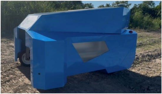
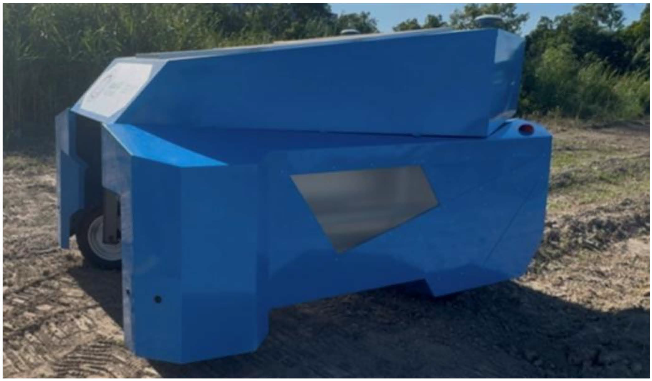
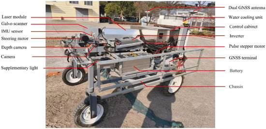
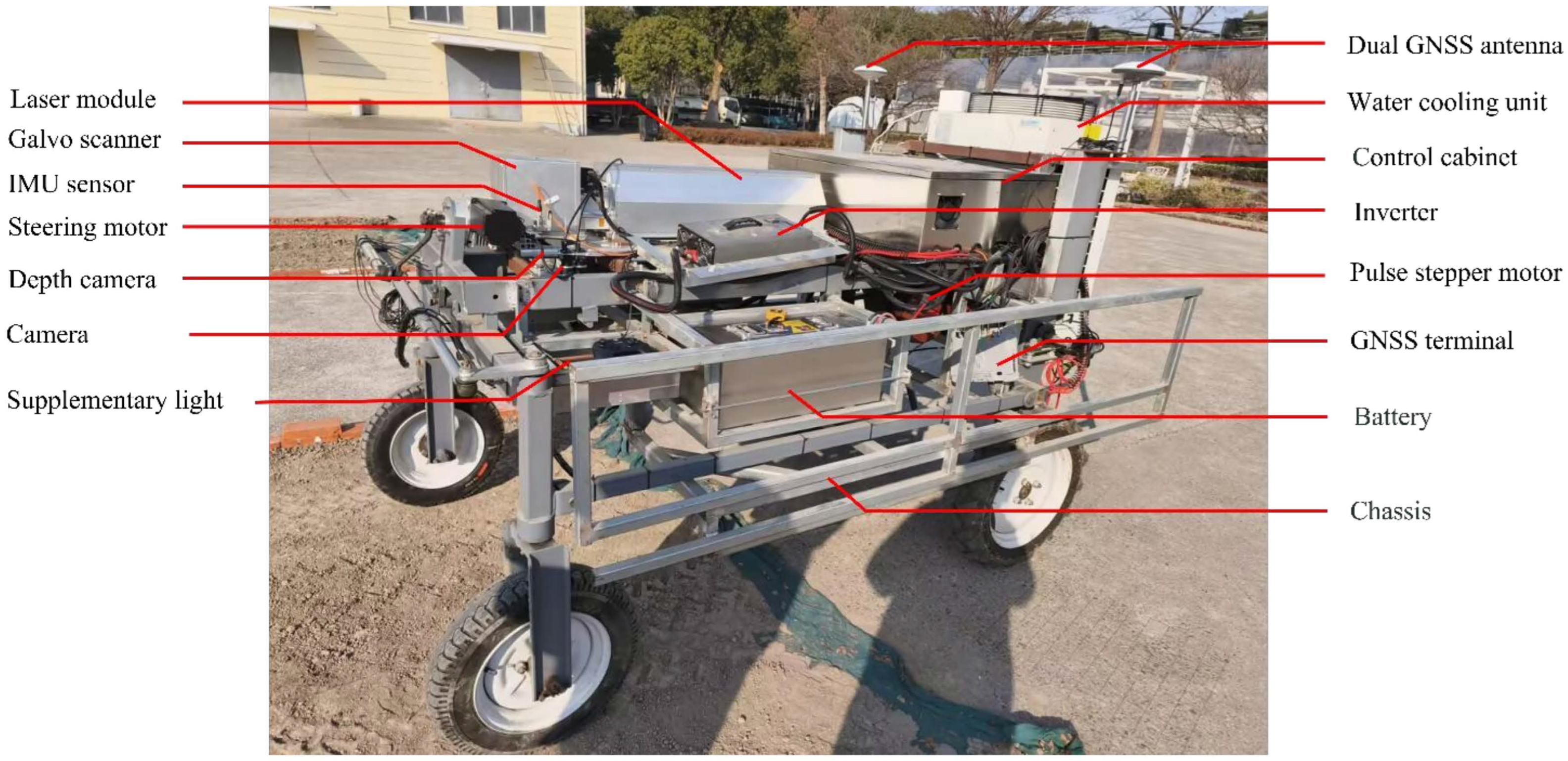
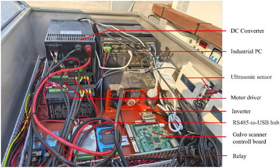
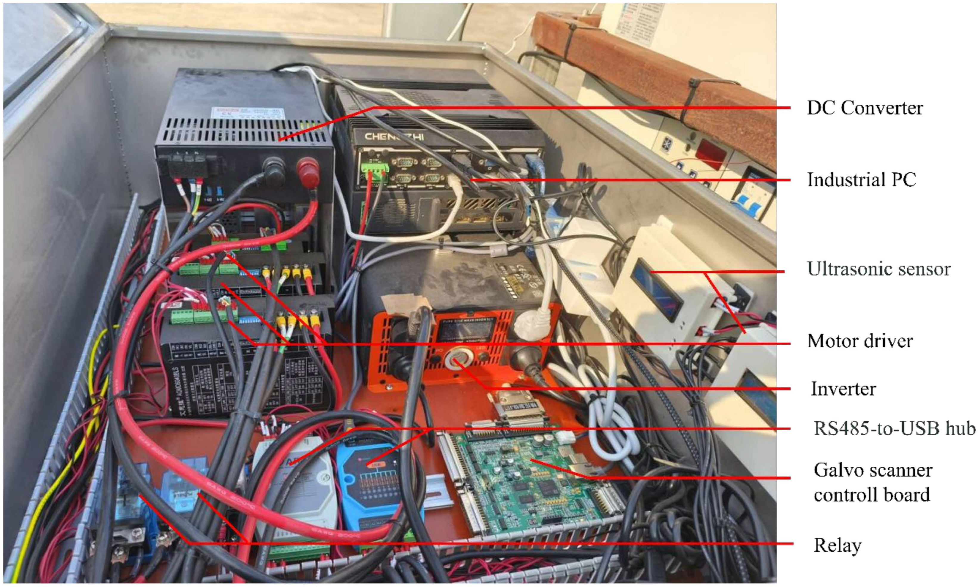
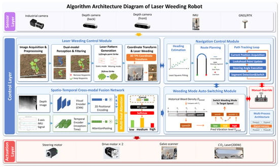
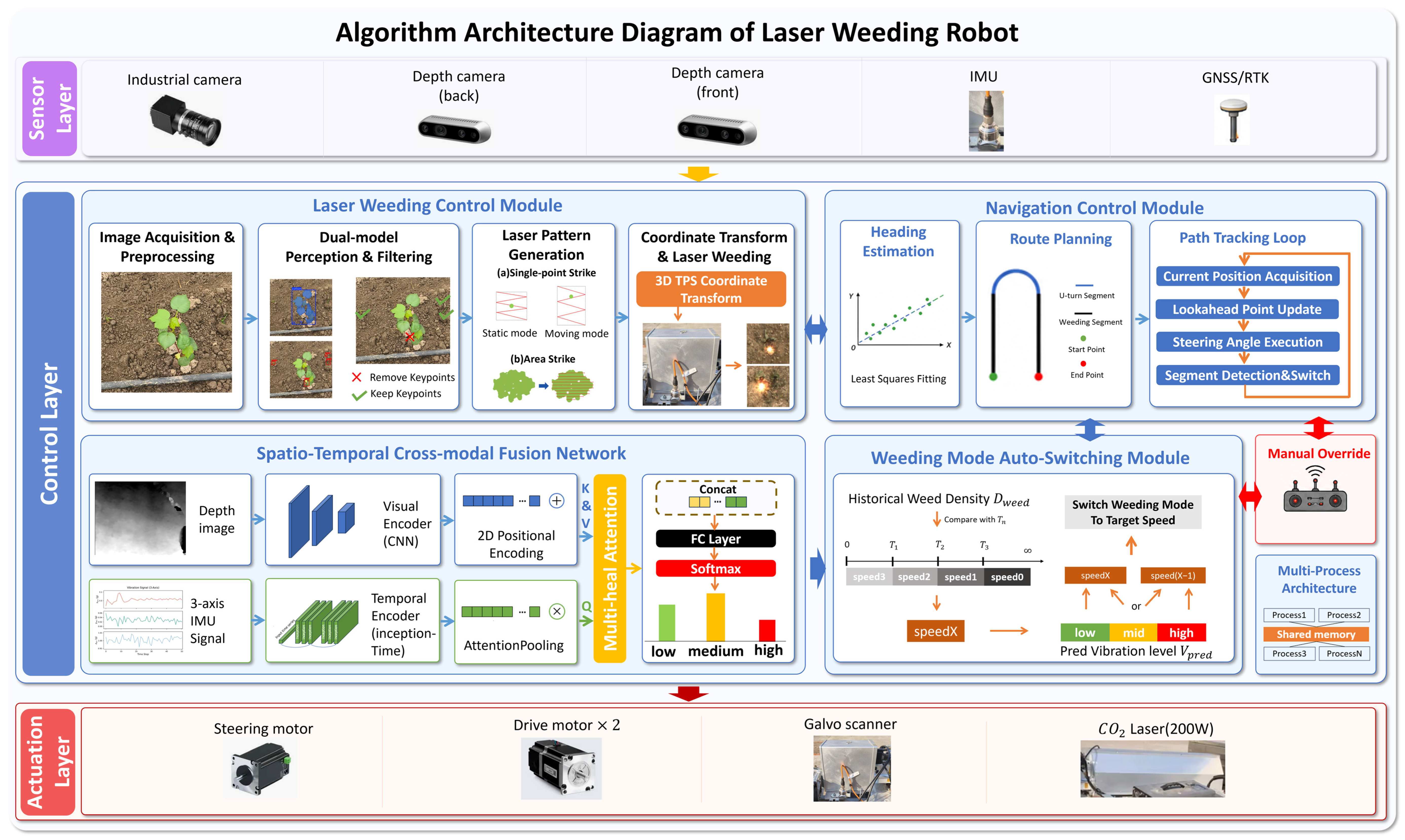
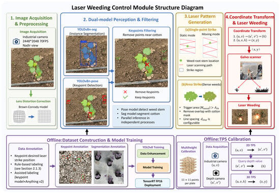
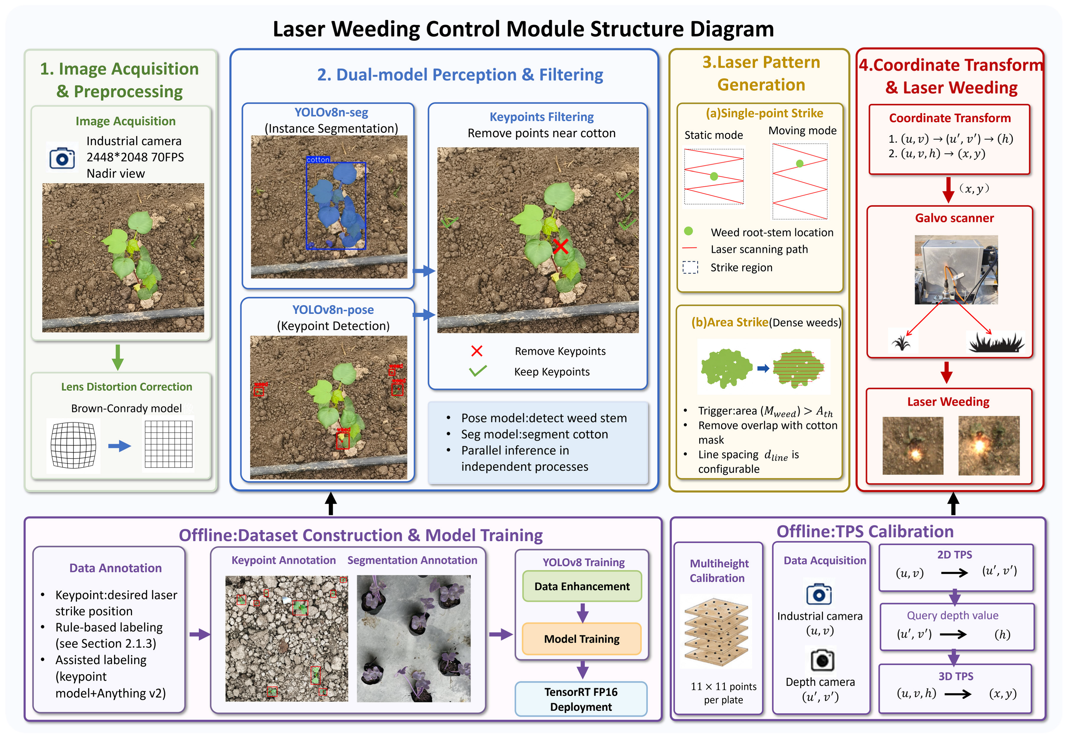
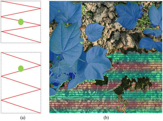
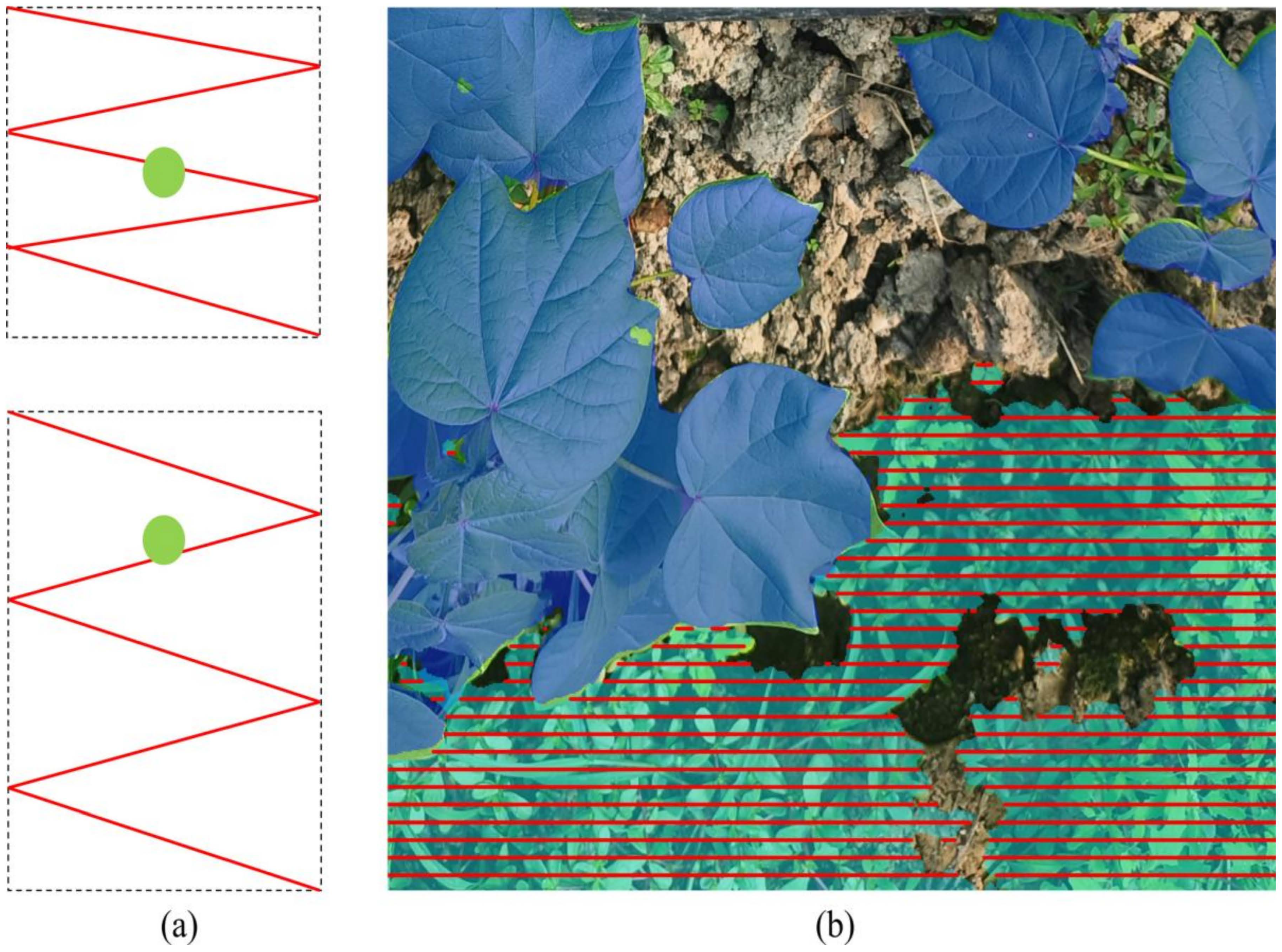
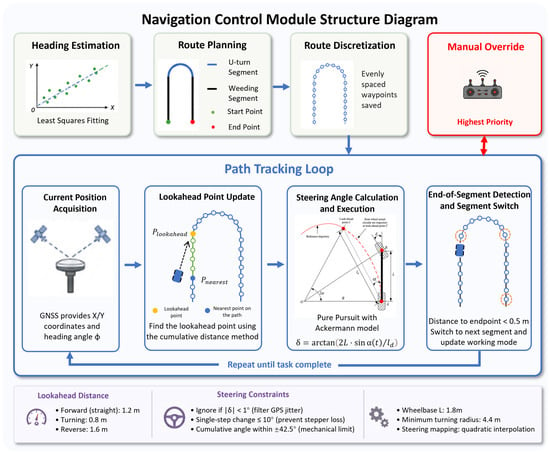
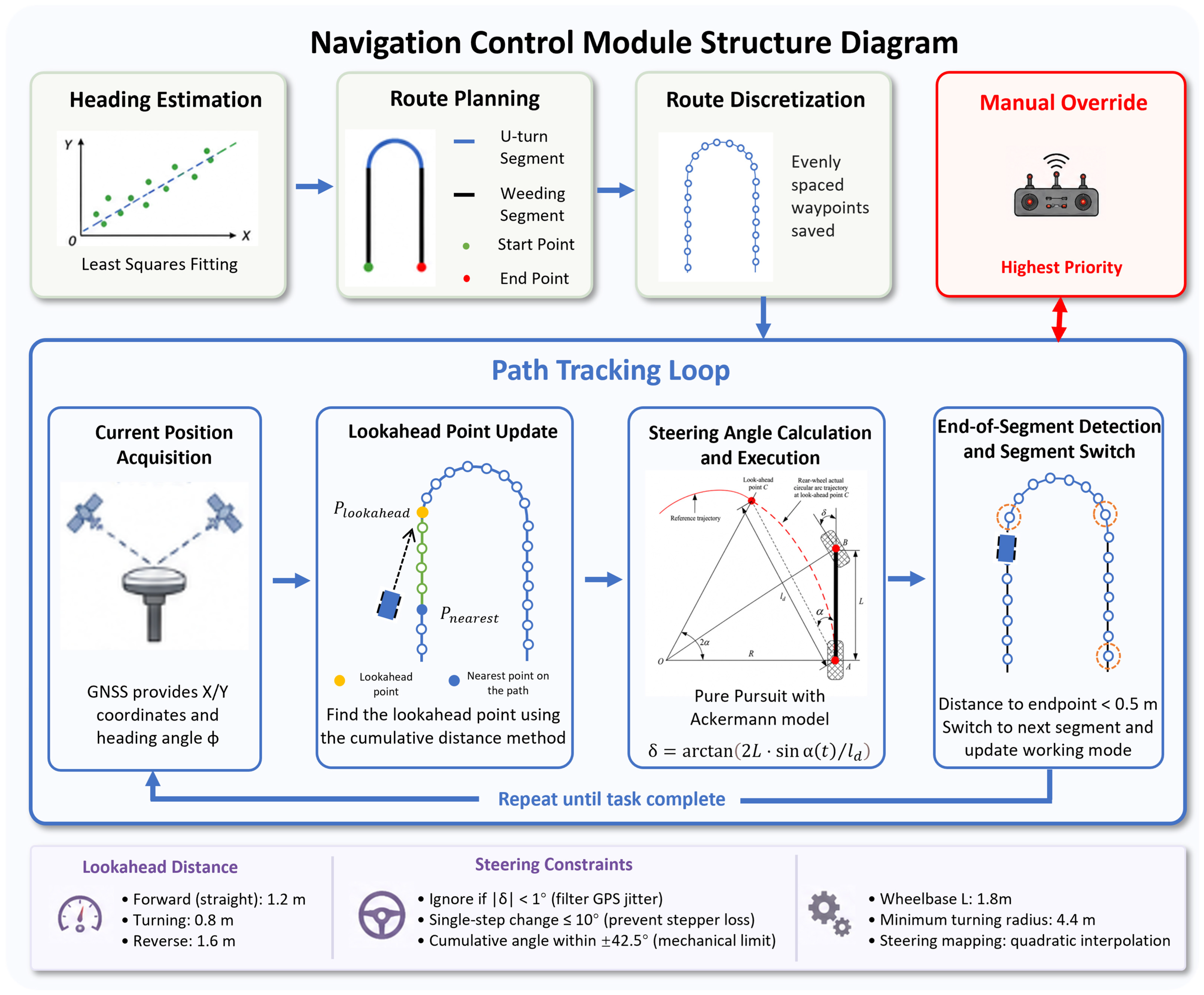
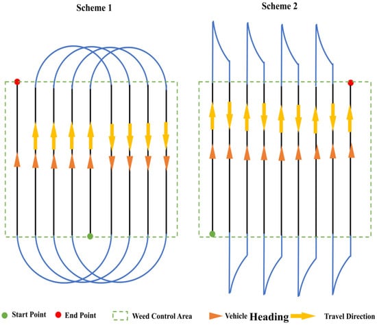
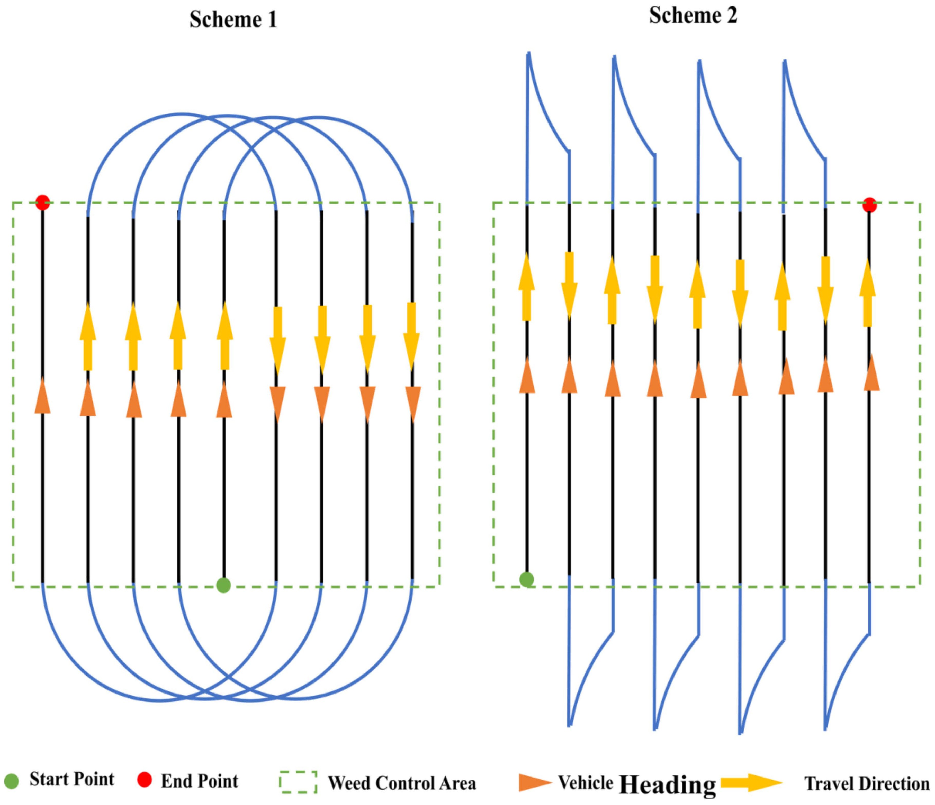
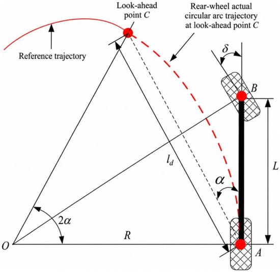
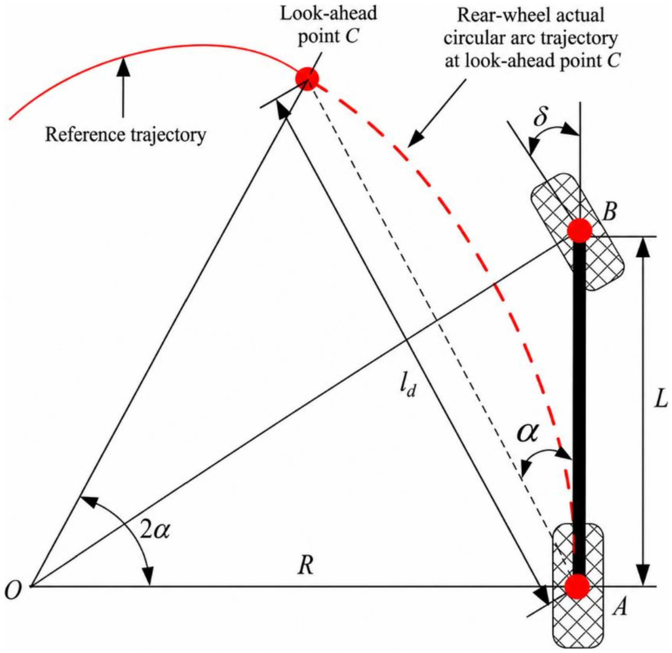
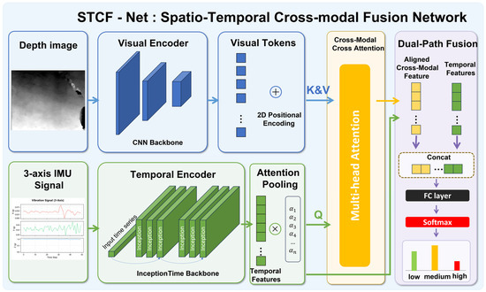
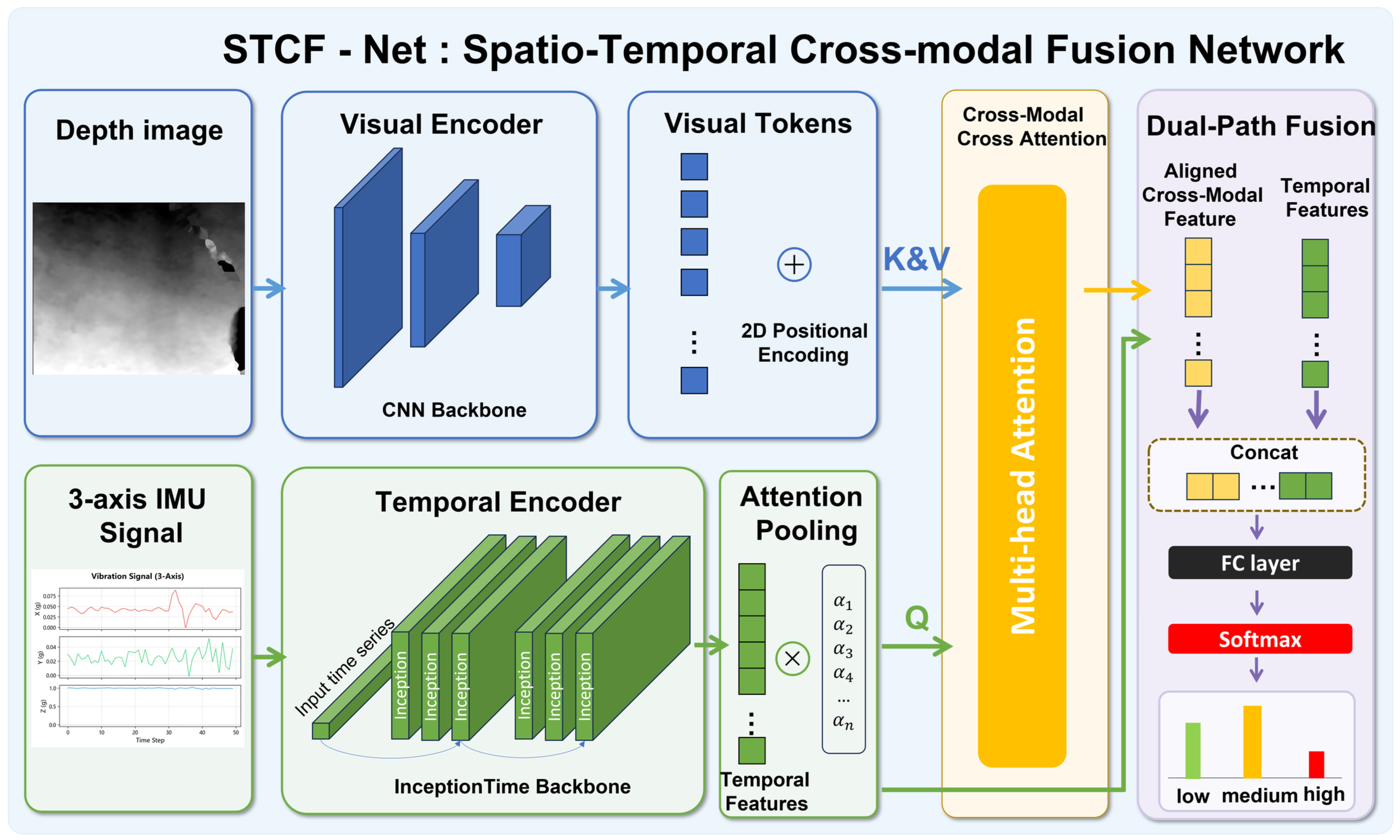
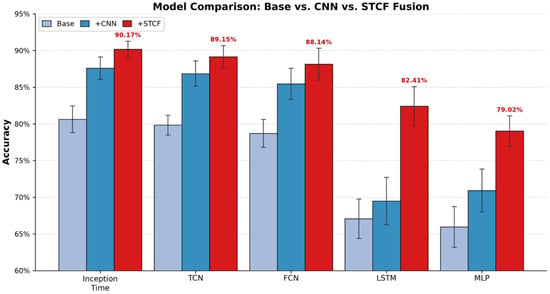
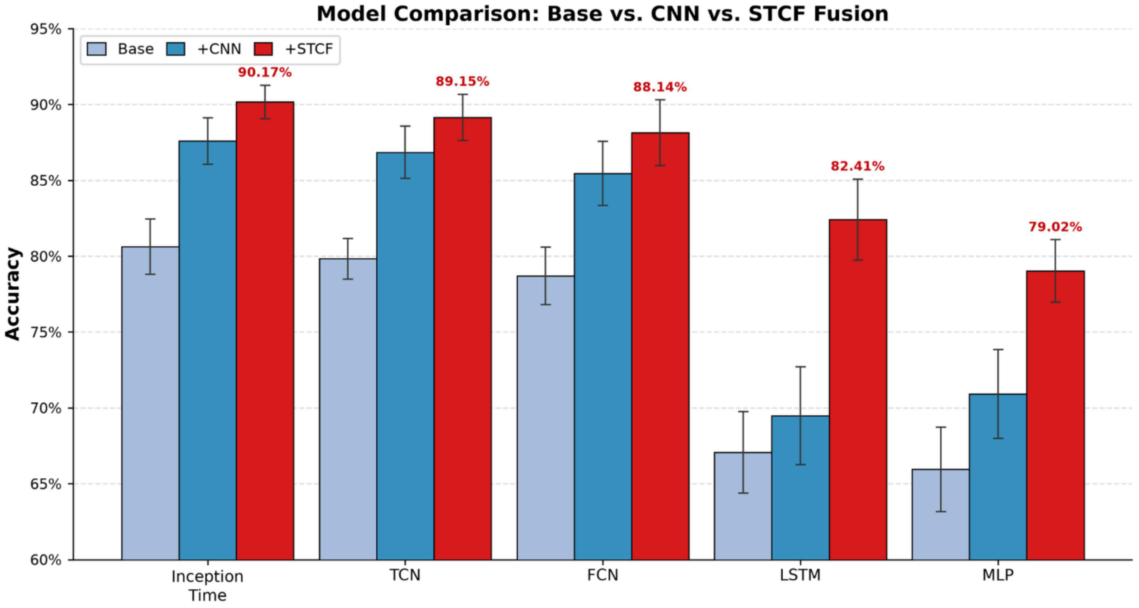
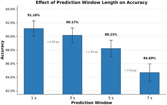
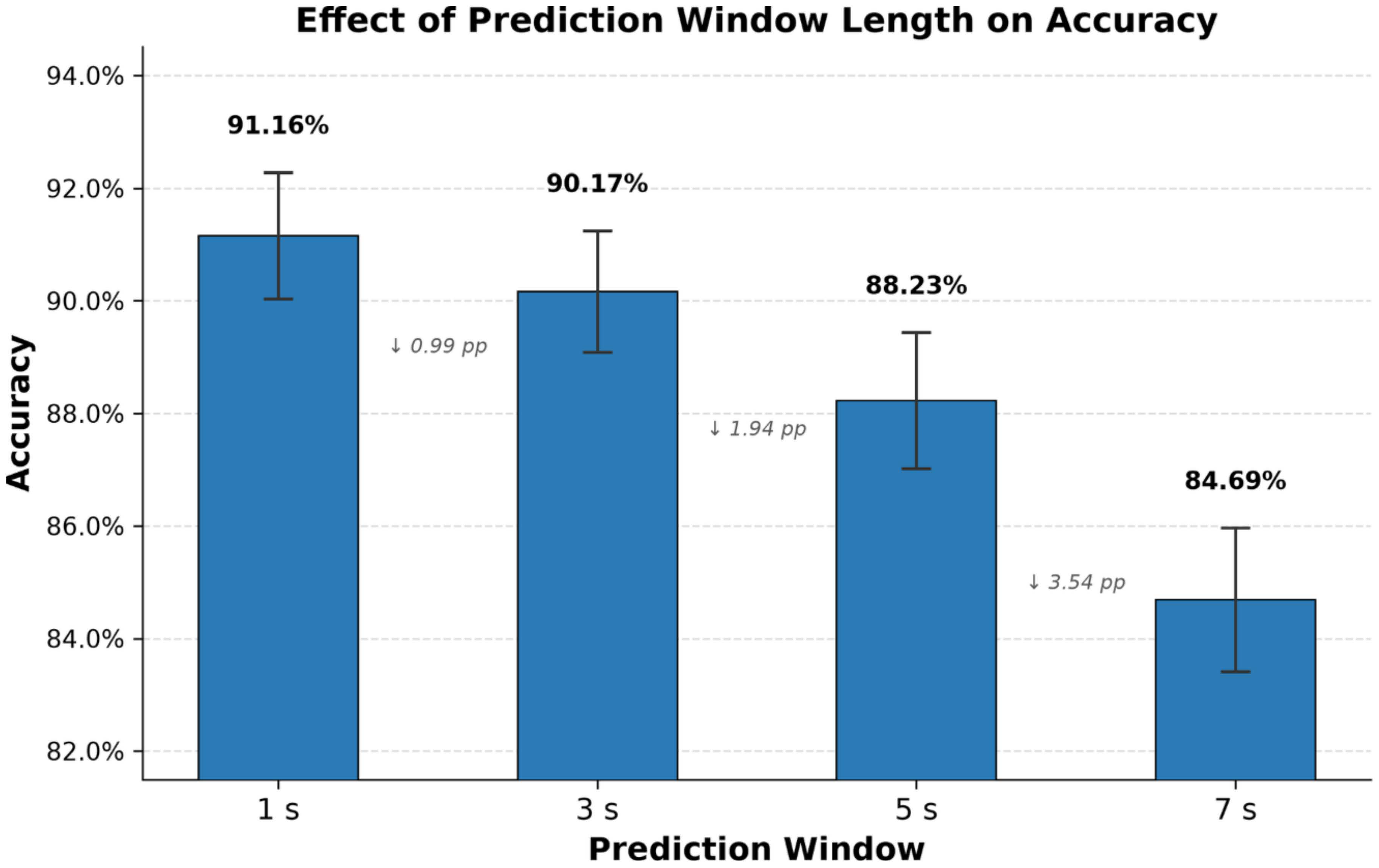
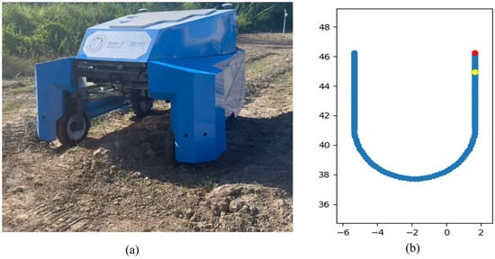
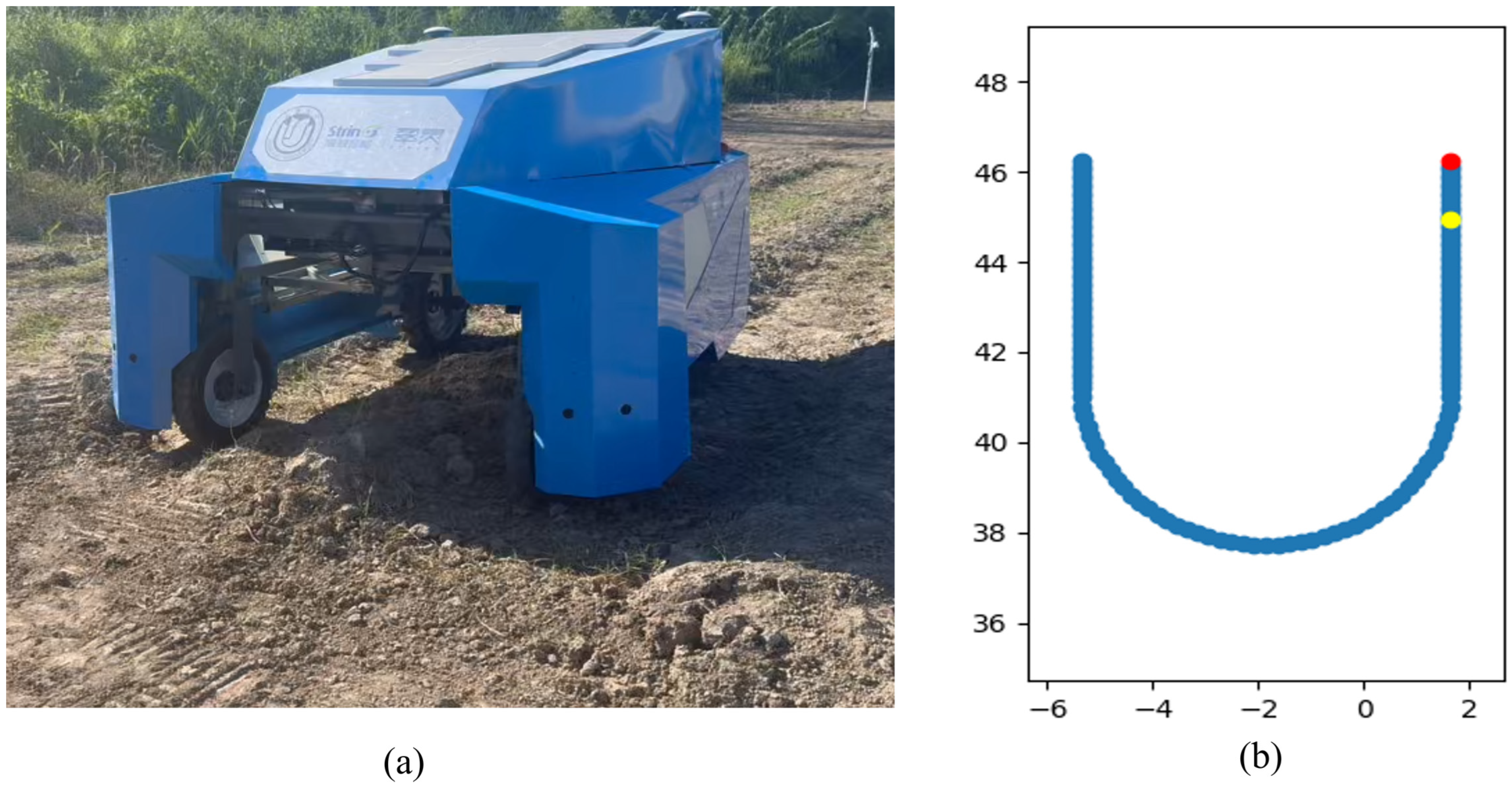
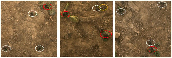
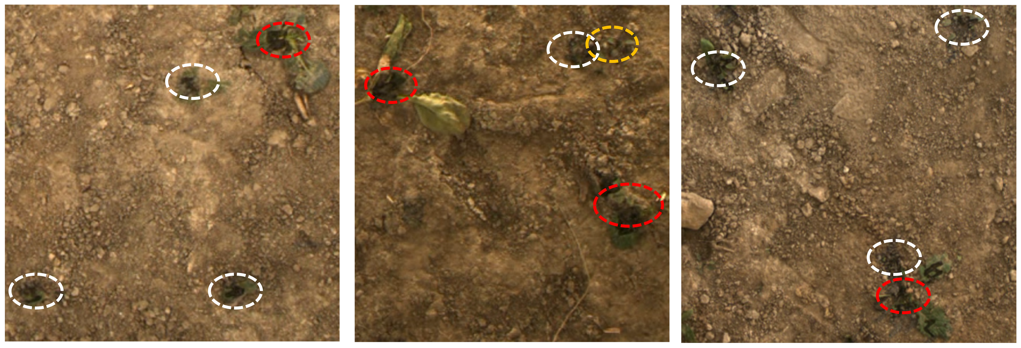
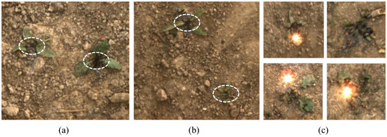
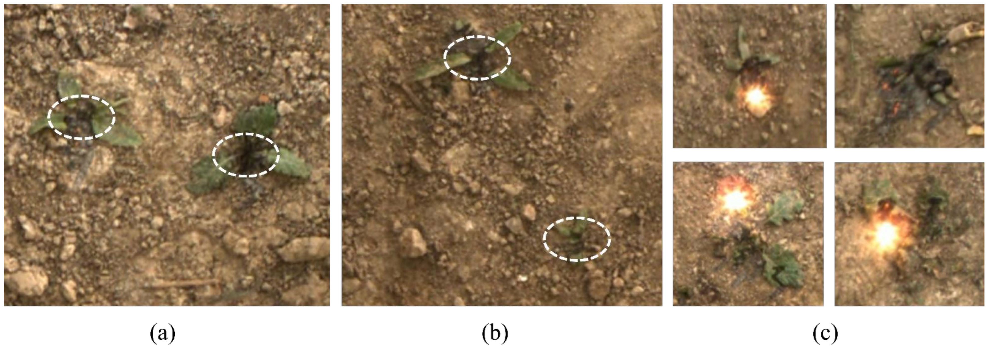
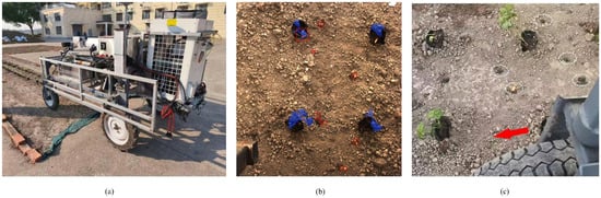
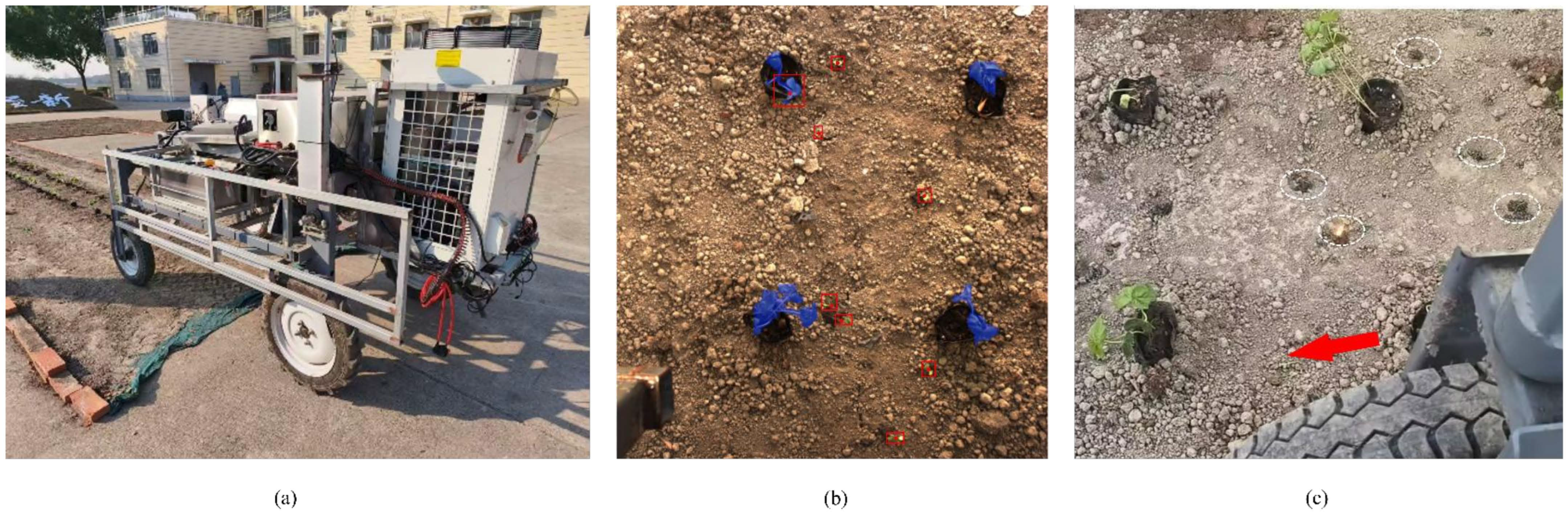
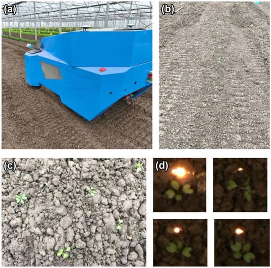
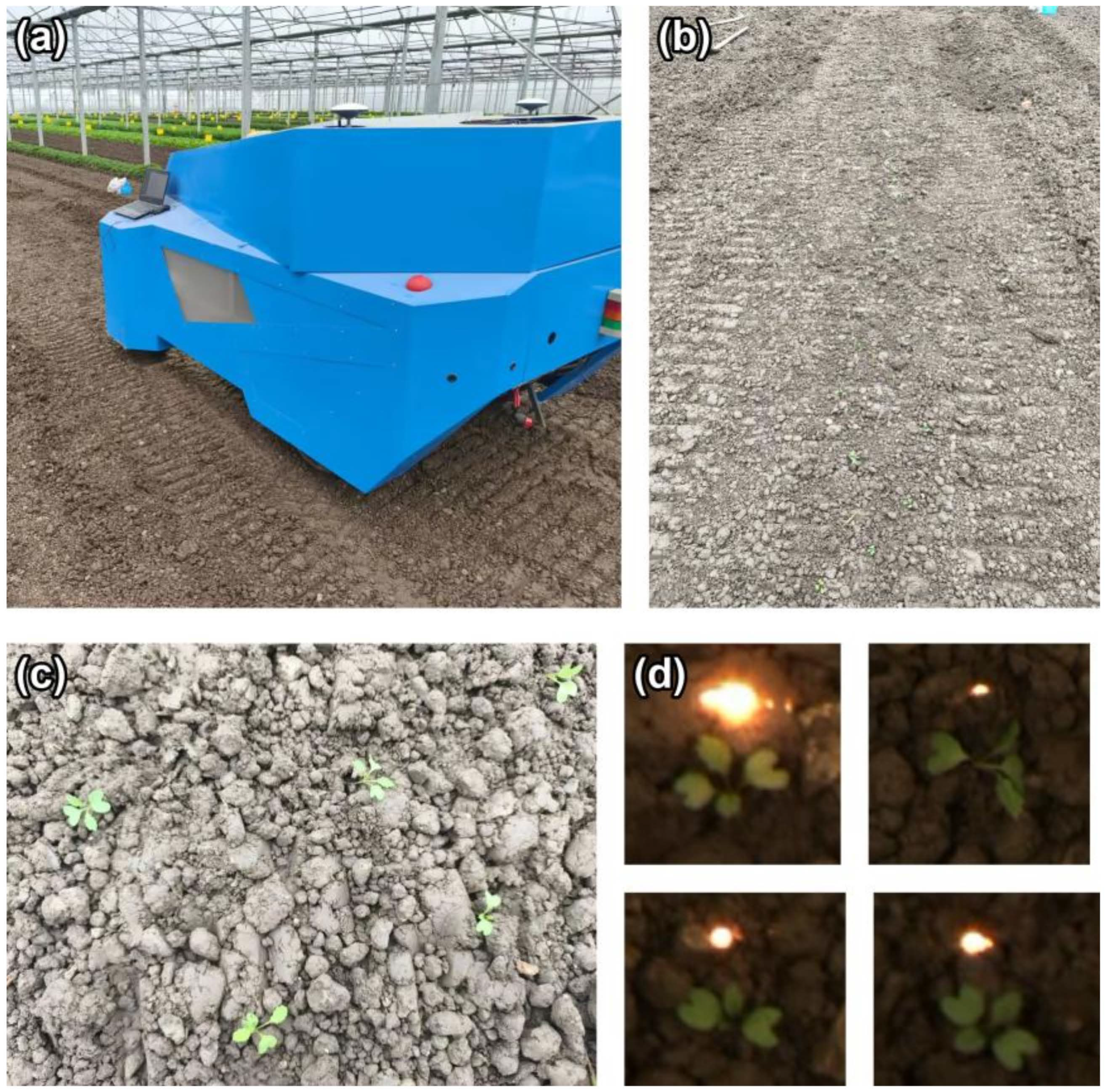

Disclaimer/Publisher’s Note: The statements, opinions and data contained in all publications are solely those of the individual author(s) and contributor(s) and not of MDPI and/or the editor(s). MDPI and/or the editor(s) disclaim responsibility for any injury to people or property resulting from any ideas, methods, instructions or products referred to in the content. |
© 2026 by the authors. Licensee MDPI, Basel, Switzerland. This article is an open access article distributed under the terms and conditions of the Creative Commons Attribution (CC BY) license.