


Abstract
Estimating fresh biomass prior to harvest can facilitate the planning of lavender harvesting. This study assessed the integration of UAV-RGB visual and numerical data using 459 original images, representing 287 plant-year units from three distinct field-year campaigns. A fixed grouped partition facilitated 135 runs across five input/fusion groups, nine backbones, and three training seeds. The Model17-FiLM demonstrated a seed-level mean R2 of 0.934 ± 0.010 and an RMSE of 178.2 ± 13.8 g, in contrast to the RGB-only Base model, which showed 0.910 ± 0.021 and 208.4 ± 25.6 g. When predictions were averaged across all nine backbones and three seeds, the RMSE decreased from 196.78 g for the Base model to 166.27 g for Model16 and 163.32 g for Model17-FiLM. Pointwise bootstrap intervals indicated the benefit of incorporating the descriptor branch, although the contribution to harvest timing remained uncertain. FiLM produced lower point-estimate errors compared to concatenation, without consistent multiplicity-adjusted support. The numerical-only RF17 model resulted in an RMSE of 423.52 g. Model21 did not enhance predictive accuracy and included redundant nominal scale inputs. The restriction to persistent plants maintained the principal ranking, while audits of acquisition sessions and markers revealed contextual sensitivity. Expanded Grad-CAM analysis demonstrated a strong dependence on the backbone. These findings endorse the evaluated approach within this dataset, though caution is advised against general deployment without independent validation across different field-years.
1. Introduction
Lavender (Lavandula × intermedia) is a perennial crop used to produce high-value essential oils and aromatic products [1]. Accurate pre-harvest fresh biomass estimation supports planning of distillation capacity, labor requirements, and transportation. Conventional cutting and weighing provides a direct reference measurement but requires destructive sampling and substantial labor at field scale. Image-based methods offer a non-contact alternative for estimating crop mass. For example, Rodríguez-Álvarez et al. [2] reported non-destructive weight estimation in cactus crops using a YOLOv5-based image-processing pipeline. In earlier lavender research, volumetric and image-derived features extracted from DJI Mavic Air imagery acquired with a standard RGB (red, green, blue) camera were modeled using Random Forest regression, with group-based data partitioning [3].
Related UAV-RGB phenotyping workflows also combine plant-object extraction with engineered morphological descriptors. Li et al. [4] used vegetation segmentation and morphological features with Random Forest classification to estimate potato emergence. This provides methodological context for object-based image analysis, although emergence counting is not directly comparable with harvested fresh biomass regression.
Research on non-destructive biomass and yield estimation has progressed from spectral indices to end-to-end image representations and multisource fusion. Proximal RGB-D imagery combined with end-to-end deep learning has enabled plant-biomass monitoring at high temporal resolution under controlled conditions [5]. In UAV (unmanned aerial vehicle) studies, combining RGB, multispectral, and structural information can provide complementary information for targets such as maize biomass and wheat yield [6,7]. End-to-end soybean yield estimation with a 3D-CNN using plot-scale, multitemporal UAV-RGB sequences has also demonstrated the predictive information available from RGB observations alone [8]. Conversely, the performance of conventional machine-learning methods using selected spectral and textural features in konjac illustrates that model performance depends on data representation and sampling design, rather than architecture alone [9].
Providing numerical inputs alongside learned visual representations allows phenological, environmental, or phenotypic context to be represented explicitly. Studies of rice, soybean, and maize yield have shown that joint modeling of images or time series with environmental and phenotypic variables can provide complementary information [10,11,12]. Integrating phenotypic traits with image-derived features has also improved wheat-yield prediction during maturation [13]. Optical and phenotypic metrics have been combined for rapeseed aboveground-biomass mapping, while genomic–phenomic fusion has im-proved grain-yield prediction in wheat breeding [14,15]. In the present study, visual–numerical fusion primarily denotes the integration of features learned from RGB images with engineered numerical descriptors derived from the same images and a harvest-timing covariate, rather than fusion of different sensor modalities. Additional variables may be redundant, linearly dependent, or associated with contextual relationships specific to a data partition. Because flight altitude and sampling strategy can influence UAV-RGB-based estimation, scale-related information requires controlled evaluation [16].
The primary research question was whether adding numerical context through Feature-wise Linear Modulation (FiLM) reduced fresh biomass prediction error relative to an RGB-only model with the same visual branch. The primary experiment compared Base, Model17-FiLM, and Model21. Mod-el17-FiLM combined the RGB representation with 16 image-derived texture, color, geometric, and structural descriptors and the calendar-day interval between image acquisition and harvest. Model21 additionally incorporated DJI metadata-derived relative altitude and three nominal scale-derived variables. The primary hypothesis concerned the Base-to-Model17-FiLM improvement, and the secondary question concerned the incremental value of the Model21 scale block.
Additional analyses were introduced during revision without changing the fixed data partition. Model16 retained the 16 image-derived numerical descriptors but omitted HasatOncesiGunSayisi. Model17-Concat used the same available visual and numerical information as Model17-FiLM but fused the embeddings by concatenation. RF17 evaluated the same 17 numerical inputs without a learned RGB representation. Equal-weight averaging of all nine backbones assessed dependence on backbone subset selection. Persistent-plant restriction, scale-variable correlations, acquisition-session audits, marker occlusion, and multi-backbone Grad-CAM addressed complementary aspects of robustness and interpretability. The primary experiment and the revision-stage analyses are distinguished throughout the reporting.
Relative to the earlier lavender study [3], which used 224 RGB images from 64 plants and Random Forest regression, the present study evaluates 459 original images from 287 plant-year units across three field-year campaigns. The methodological extension lies in the shared CBAM–GeM visual branch, controlled numerical-input and fusion comparisons, nine pretrained backbones, three training seeds, and a fixed Kok_id-grouped evaluation protocol. Model16 evaluates the conditional addition of harvest timing, whereas Model17-Concat tests an alternative fusion operation using the same inputs. These extensions support within-dataset assessment of model design and nominal scale information, not a new invention of FiLM or a direct performance ranking against the earlier dataset.
2. Materials and Methods
2.1. Dataset, Field Protocol, and Kok_id-Based Sampling Design
The dataset comprised 459 original, approximately nadir UAV-RGB images representing 287 plant-year units (Kok_id) from three campaigns in Türkiye: Uşak-2024 (n = 64), Uşak-2025 (n = 48), and Burdur-2025 (n = 175). Both sites were open-field plantations in field soil. Field records identified the plant material as Lavandula × intermedia, but cultivar-level identification was unavailable. The Uşak plantation was established during 2020–2021, whereas the Burdur plants were five years old during the 2025 campaign. Harvesting at both sites began in the third growing year. Uşak-2024 corresponded to the second harvest cycle, and Uşak-2025 and Burdur-2025 to the third, with one, two, and two previous harvests, respectively.
For public reporting, site coordinates are deliberately masked as 38.XXXX° N, 29.XXXX° E for Uşak and 37.XXXX° N, 30.XXXX° E for Burdur. The decimal digits are withheld to protect the precise field locations. These masked strings are geographic context only and are not reproducible extraction coordinates. The unmasked coordinates supplied for the study were used for the meteorological queries but are not published here.
The described planting layout at Uşak comprised five rows, each containing three sections of equal planted area. Within each row, one-third of the planted area had a spacing of 3 × 1 m, one-third had a spacing of 3 × 2 m, and the remaining one-third had a spacing of 3 × 3 m. Thus, all three spacing arrangements were present within every row. Burdur had an approximately square 1.8 × 1.8 m planting arrangement. These spatial arrangements are reported as field characteristics. Planting spacing was not included as a model predictor or evaluated as a treatment factor in the present analysis.
Under an idealized, fully occupied rectangular layout, nominal planting density was calculated as 10,000 divided by the product of the two spacings in meters. The 3 × 1 m, 3 × 2 m, and 3 × 3 m arrangements correspond to approximately 3333, 1667, and 1111 plants ha−1, respectively. Because each spacing occupied one-third of the planted area within every Uşak row, the area-weighted nominal density of the described five-row layout was approximately 2037 plants ha−1. The approximately 1.8 × 1.8 m Burdur arrangement corresponds to approximately 3086 plants ha−1. These calculations assume full occupancy and disregard missing plants, boundary effects, and non-planted areas. They describe nominal planting density rather than measured stand density. Equal area allocation does not establish equal representation of the spacing classes among the sampled Kok_id units. Per-hectare biomass and field-total prediction error were not evaluated.
Neither irrigation nor fertilization was applied at either site, and no agricultural pesticides or mulch were used. Routine management consisted primarily of periodic mechanical cultivation between rows. The same absence of the listed inputs applied at both sites, but identical cultivation dates, depth, or intensity were not established. The available Türkiye Ulusal Coğrafi Bilgi Sistemi (TUCBS) soil information [17] described the Uşak site as brown forest soil and the Burdur site as brown soil, with medium-textured loamy soils at both locations. These are map-based site descriptions rather than laboratory soil measurements. Approximate elevations were 866 and 1030 m a.s.l., respectively. Terrain slopes were estimated at approximately 14% and 3.21% from elevation differences and horizontal distances obtained from web-based mapping resources. These values describe the sites approximately and are not survey-grade measurements.
Meteorological conditions were characterized retrospectively using ERA5-Land [18] and the ERA5 Land hourly time-series product in the Copernicus Climate Data Store [19], rather than direct plot-level measurements. The dataset identifier was reanalysis-era5-land-timeseries. Site-coordinate queries were assigned to the nearest available grid point. The reference window extended from 1 March through the recorded harvest date, inclusive, rather than from an observed biological growth-onset date. The extraction-run summaries reported mean 2 m air temperatures and total precipitation of 18.60 °C and 126.71 mm for Uşak-2024, 17.48 °C and 141.35 mm for Uşak-2025, and 16.26 °C and 221.12 mm for Burdur-2025, respectively. These quantities describe the campaign environments and were not included as model predictors.
An integrated RGB camera on a DJI Mavic Air (DJI, Shenzhen, China) UAV was used throughout the campaigns. Uşak-2024 images were acquired on 13, 19, 28, and 29 July before harvest on 1 August 2024, corresponding to image-to-harvest intervals of 19, 13, 4, and 3 days, respectively. Uşak-2025 images were acquired on 18 July before harvest on 28 July 2025, giving a 10-day interval. Burdur-2025 images were acquired on 19 July before harvest on 25 July 2025, giving a 6-day interval. These recorded intervals defined HasatOncesiGunSayisi. Campaign details are summarized in Table 1.
Table 1.
Field-year context, image acquisition, and recorded harvest dates. Spatial information is deliberately masked, and nominal densities are not measured stand counts.
The harvest cut was made at an approximate height corresponding to one-third to two-fifths of total plant height above the soil surface, consistent with the general practice used in previous harvests. This proportion denotes the height of the cut above the soil, not the fraction of canopy removed. The harvested flower and stem fractions were weighed together within 2 h of cutting. Each plant had one recorded fresh-mass reference. Fresh mass (YasAgirlikGr, g) was measured using a Dmax 4219 (Dmax Global, İstanbul, Türkiye) handheld digital scale with a 0–10 kg weighing range and 5 g readability. The scale was reset to zero before each measurement. Two identical devices were available, and intermittent comparisons with the second device provided field consistency checks. Calibration using certified reference weights was not performed, and replicate weighings were not systematically recorded. Consequently, empirical repeatability and instrument-related measurement uncertainty could not be quantified retrospectively. The harvested target was not the entire standing plant, and woody material was not quantified separately. Dry biomass was also measured during the broader field campaign but was excluded from the present fresh biomass analysis.
Visual identification markers were used to link plant images to harvest records. The markers were not systematically removed during cropping and remained visible in some images. Their potential influence on the visual branch was assessed using the marker-occlusion analysis described in Section 2.7.
A 1024 × 1024-pixel plant-centered crop was extracted from each source image without geometric resampling. Surrounding soil, vegetation, and identification markers could remain visible. The resulting PNG images were resized to 224 × 224 pixels using OpenCV (4.13.0 ver.) INTER_AREA. During training, each original image was used together with nine augmented derivatives [20]. The augmentation operations were bright09/bright11 (pixel-intensity multiplication by 0.9 and 1.1, respectively), contrast09/contrast11 (contrast coefficients of 0.9 and 1.1 applied around the grayscale mean of the entire image), crop05 (removal of approximately 5%, or 11 pixels, from each edge of the 224 × 224 image, followed by extraction of the central 202 × 202 region and resizing to 224 × 224), hflip, vflip, rot90, and rot270. The 16 image-derived features were recalculated for each augmented image rather than copied from the original. For crop05, propagation of the scale-derived variables accounted for the reduced field of view. Validation and test images underwent the same plant-centered cropping and resizing, but no augmentation was applied. Augmentation was used to address constraints on the number of obtainable field samples, consistent with its reported use in remote-sensing-based yield modeling [21]. For nominal GSD propagation, cropping from the native-resolution images preserved the per-pixel scale because the source PNG images were not geometrically resampled before cropping. Resizing the 1024 × 1024 crop to the 224 × 224 model input changed the nominal scale per pixel by a factor of 1024/224.
The analysis unit, Kok_id, combined the study site, harvest year, and the root number assigned in the field. Of the 287 units, 217 were represented by one original image and 70 by two to ten original images. The test partition contained 21 single-image units and eight multi-image units, giving 29 Kok_id units and 46 original images. All original images and training augmentations associated with a given Kok_id remained within the same partition. Accordingly, all pairwise intersections among the training, validation, and test partitions were zero at the Kok_id level.
A root number recurring in a different year received a distinct year-specific Kok_id because it represented a separate seasonal observation and harvest. This definition does not establish biological independence of perennial plant positions across years. Cross-year overlap was therefore examined separately using PersistentID, defined as site plus root number. Plant inclusion depended on the feasibility of acquiring an individually identifiable image and linking it unambiguously to a harvest record. Consequently, the sample did not arise from a formally randomized field-sampling frame. Table 2 summarizes the fixed data partition.
Table 2.
Main characteristics of the fixed data partition.
There was no Kok_id overlap among the partitions. In the training partition, 362 original images were expanded to 3620 model records together with their nine derivatives. In the validation and test partitions, 51 and 46 original images were evaluated, respectively. The field-year and root-based distributions for Burdur-2025/Uşak-2024/Uşak-2025 were 137/49/43 in the training set, 20/8/1 in the validation set, and 18/7/4 in the test set. The DJI metadata-derived relative-altitude ranges were 0.2–5.8 m for training, 0.7–5.8 m for validation, and 0.9–4.2 m for testing. The corresponding nominal GSD proxy ranges were 0.0309–0.8963, 0.1082–0.8963, and 0.1391–0.6490 cm pixel−1. The source-record audit reported numerical correspondence between the dataset altitude and DJI RelativeAltitude/EXIF altitude records for all 459 original images. DJI AbsoluteAltitude was not used. These values refer to the take-off reference, not to directly measured camera-to-canopy distance. The partition remained fixed across all model groups and training seeds. Because the test target range was 72–2785 g, whereas the training set extended up to 4480 g, the locked test evaluation did not fully cover the highest-biomass range of the training distribution.
2.2. Image Processing and Numerical Features
Before generating the plant mask, a 5 × 5 Gaussian blur was applied, after which CLAHE (Contrast Limited Adaptive Histogram Equalization [22]; clipLimit = 2.0; tileGridSize = 8 × 8) was applied to the L channel in the LAB (CIE L*a*b*) color space, and the image was converted to the HSV (Hue, Saturation, Value) color space. Thresholds of [25, 10, 10]–[95, 255, 255] for the green region and [115, 10, 10]–[175, 255, 255] for the purple region were combined. Opening and closing operations were applied using a 7 × 7 elliptical structuring element, and the largest external contour was selected as the plant object. The stages of image processing, masking, and plant-boundary extraction are illustrated for selected samples in Figure 1.
Figure 1.
Image-processing and masking outputs for five lavender samples, arranged by row. For the first sample, (a) shows the original RGB image, (b) the HSV-masked RGB image, and (c) the segmented plant with its convex-hull boundary. For the second sample, (d) shows the original RGB image, (e) the HSV-masked RGB image, and (f) the segmented plant with its convex-hull boundary. For the third sample, (g) shows the original RGB image, (h) the HSV-masked RGB image, and (i) the segmented plant with its convex-hull boundary. For the fourth sample, (j) shows the original RGB image, (k) the HSV-masked RGB image, and (l) the segmented plant with its convex-hull boundary. For the fifth sample, (m) shows the original RGB image, (n) the HSV-masked RGB image, and (o) the segmented plant with its convex-hull boundary. HSV masking followed Gaussian blurring and CLAHE. Final segmentation involved elliptical morphological opening and closing, followed by selection of the largest external contour.
The texture features were calculated from valid pixel pairs within the mask using a symmetric and normalized GLCM (Gray-Level Co-occurrence Matrix) with 32 gray levels, d = 1 pixel, and directions of 0°, 45°, 90°, and 135°, and the directional values were combined using the arithmetic mean [23,24]. The 16 image-derived features used in Model17-FiLM were Contrast, Correlation, Homogeneity, Energy, R_mean, G_mean, B_mean, H_mean, S_mean, V_mean, Entropy_gray (grayscale entropy), area_px, perimeter_px, form_factor, solidity, and EdgeDensity. The RGB/HSV channel means were calculated within the mask, and grayscale entropy was obtained as base-2 Shannon entropy from an 8-bit histogram. The geometric and edge-related variables were area_px (A), perimeter_px (p), form_factor, solidity, and EdgeDensity, as defined in Equation (1), where Ahull denotes the convex hull area, Nedge denotes the number of edge pixels within the mask, and Nmask denotes the number of mask pixels.
Model17-FiLM used the 16 image-derived descriptors together with HasatOncesiGunSayisi, defined as the calendar-day interval between image acquisition and the recorded harvest date. This variable is a harvest-timing covariate, not a directly observed phenological stage or the prediction target. Model16 retained the same 16 descriptors and FiLM architecture but excluded this covariate. The Base-to-Model16 comparison therefore evaluates the addition of the engineered-descriptor branch with FiLM, whereas the Model16-to-Model17-FiLM comparison evaluates the incremental value of harvest timing conditional on that branch. This sequential ablation does not estimate a timing-only effect or a full factorial interaction.
Model21 appended four metadata-derived variables to the Model17-FiLM input: relative altitude (UcusYuksekligi_m), the nominal model-space GSD proxy (GSD_224_theoretical_cm_px), scaled area (area_gsd_cm2), and scaled perimeter (perimeter_gsd_cm). The native-image proxy was calculated using Equation (2):
Here H denotes DJI metadata-derived relative altitude in meters, Sw = 6.17 mm is sensor width, f = 4.5 mm is focal length, and Iw = 4056 pixels is the native image width used in the calculation. The factor 100 converts meters to centimeters. Cropping to 1024 × 1024 pixels without resampling preserves the nominal per-pixel scale. Resizing that crop to the 224 × 224 input gives Equation (3):
The model-space proxy is therefore 1024/224 times the native-image proxy. Metadata-scaled area and perimeter were calculated using Equation (4):
These quantities are nominal metadata-derived scale proxies, not measurements calibrated using GCPs, orthophotos, or a DEM. They do not account for canopy height, terrain variation, or elevation differences between the take-off reference and the target canopy. Therefore, area_gsd_cm2 and perimeter_gsd_cm do not represent independently calibrated physical plant dimensions. With fixed camera constants, relative altitude and the nominal GSD proxy are deterministically proportional. Their individual contributions cannot be inferred from the four-variable block comparison. The four-variable block is retained as the originally evaluated Model21 condition, rather than a recommended set of independent predictors. The correlation analysis characterizes that evaluated representation and does not justify retrospectively redefining the tested model. Table 3 defines the numerical inputs and their inclusion in each model group.
Table 3.
Numerical input definitions and inclusion across the evaluated fusion models.
2.3. Controlled Model Groups and Fusion Architecture
Nine ImageNet-pretrained backbones were evaluated: ResNet50/101/152, DenseNet169, InceptionV3 [25], MobileNetV3Large, and EfficientNetB0/B1/B7 [26,27,28,29,30]. Each backbone was used in the three primary model groups and the two additional controls. In the shared visual branch, the backbone output was followed by a CBAM (Convolutional Block Attention Module) block with a channel-reduction ratio of 8 and a 7 × 7 spatial convolution, learnable Generalized Mean (GeM) pooling initialized with p = 3 and ε = 10−6, dropout at a rate of 0.25, and a 256-unit dense layer with ReLU (Rectified Linear Unit) activation [31,32,33]. GeM pooling is defined in Equation (12).
The Base model used RGB images only, omitting the numerical branch and FiLM while retaining the same CBAM–GeM visual architecture used in the fusion models. Its regression head comprised dropout at a rate of 0.25, a 128-unit ReLU layer, and a single linear output, matching the structure following FiLM in the fusion models. Thus, the Base-to-Model17-FiLM comparison evaluates the addition of numerical context without changing the visual branch. In Model17-FiLM, the numerical branch comprised a normalization layer adapted exclusively to the training data, a 64-unit ReLU layer, dropout at a rate of 0.20, and a 32-unit ReLU layer. The numerical embedding was mapped to 256-dimensional γ and β vectors. FiLM conditioning with layer normalization is defined in Equation (5) [34,35]:
The conditioned representation in Equation (5) was passed through dropout at a rate of 0.25, a 128-unit ReLU layer, and a single linear output. Model21 used this architecture with 21 numerical inputs. Model16 retained the same FiLM pathway with 16 inputs, excluding HasatOncesiGunSayisi.
Model17-Concat retained the same visual branch and the same 17-variable numerical preprocessing and embedding branch. Concatenation of the 256-dimensional visual embedding and the 32-dimensional numerical embedding produced a 288-dimensional representation, followed by layer normalization, dropout at a rate of 0.25, a 128-unit ReLU layer, and a linear output. This design provides an input-matched comparison of fusion strategies. Because the concatenated representation differs in dimension from the 256-dimensional FiLM representation, the comparison is not matched for parameter count.
Figure 2 illustrates the shared visual and numerical branches and the alternative fusion operations. Table 4 summarizes the input composition and fusion strategy of the five model groups, while Table 3 provides the numerical variable definitions.
Figure 2.
Shared visual and numerical branches and alternative fusion operations. (a) The RGB branch produces a 256-dimensional visual embedding. (b) The numerical branch produces a 32-dimensional embedding from 16, 17, or 21 inputs. FiLM generates channel-wise scale and shift vectors, whereas concatenation joins the visual and numerical embeddings before layer normalization. The Base bypasses the numerical and fusion pathways. The regression-head structure is shown below the fusion operations. Model-specific input membership is presented separately in Table 4.
Table 4.
Input composition and fusion strategy of the five evaluated model groups.
2.4. Training Protocol and Model Checkpoint Selection
The primary experiment comprised three model groups, nine backbones, and three training seeds (42, 123, and 2026), yielding 81 runs. Model16 and Model17-Concat each added 27 runs under the same backbone–seed design, giving 135 deep-learning runs in total. The Kok_id partition was generated once using split seed 42 and then frozen. Training seeds changed stochastic initialization and optimization but not partition membership. Models were trained using Adam in two stages with a batch size of 16 [36]. In the first stage, the ImageNet backbone was frozen, and training proceeded for a maximum of 100 epochs at a learning rate of 10−3. In the second stage, the final 20 backbone layers, excluding Batch Normalization layers, were unfrozen, with a maximum of 200 epochs at a learning rate of 10−4 [37]. EarlyStopping monitored val_mae_g (validation MAE in grams) with patience = 30. ReduceLROnPlateau used patience = 12, factor = 0.5, and a minimum learning rate of 10−7.
Images were retained as uint8 values in the [0, 255] range and passed to the Keras (3.13.2 ver.) preprocessing input function, which is specific to each backbone. The target variable was standardized using only the mean and standard deviation of the training partition, and Huber loss with δ = 1 was applied on the standardized scale [38]. At each stage, the checkpoint with the lowest val_mae_g was retained, and the checkpoint with the best validation MAE across the two stages was selected as the final individual model checkpoint. Individual checkpoint selection was based on image-level validation MAE, whereas ensemble selection, as described below, was based on the validation RMSE at the Kok_id level, which was the primary unit of analysis. The use of metrics at different levels in these two selection stages is noted in the limitations section. TensorFlow deterministic operations were enabled, and the training was conducted in a TensorFlow 2.20 environment on NVIDIA L4 graphics processing units (NVIDIA Corporation, Santa Clara, CA, USA).
2.5. Validation-Based Ensemble and Secondary Convex Blending
For each model group and training seed, all four-backbone subsets of the nine backbones [C(9,4) = 126] were screened using validation Kok_id predictions only. The subset with the lowest validation RMSE was retained as the primary equal-weight ensemble. Ties were resolved first by validation MAE and then by alphabetical order of the model names. Each selected backbone received a weight of 0.25, as defined in Equation (13). Test data were not used to select models, ensemble members, or weights. Nevertheless, screening 126 candidates on 29 validation Kok_id units can introduce selection optimism. The procedure was therefore treated as internal model selection rather than evidence of external generalizability. Variation in selected members across training seeds was reported as an indication of selection uncertainty.
An additional all-nine ensemble averaged the Kok_id-level predictions of all nine backbones with equal weights within each training seed. This removed backbone-subset selection, but not validation-based checkpoint selection. Predictions from the three seeds were subsequently averaged per Kok_id before calculating the across-seed prediction-mean metrics. This subset-selection-free analysis was the principal revision-stage component comparison and a complementary FiLM–Concat comparison. The component-level ablation and fusion-operator comparisons are reported in Section 3.6 and Section 3.7, respectively.
To further evaluate validation-based selection optimism, a post hoc validation sensitivity analysis was conducted without altering the primary four-model training and testing protocols. All equal-weight subsets containing 2–8 models from the same nine backbones were evaluated exclusively using the validation Kok_id predictions. For each ensemble size, the best validation Kok_id-level RMSE/MAE values were recorded, and the test predictions were not accessed.
As a secondary sensitivity analysis, a convex blend was fitted to minimize validation Kok_id-level RMSE under the specified weight constraints. This blend was not treated as the primary result. For Model17-FiLM, the optimized weight assigned to EfficientNetB1 was 1.0 under all three seeds, showing that validation-based optimization could collapse to single-backbone selection. The equal-weight ensemble was therefore retained as the primary approach.
2.6. Evaluation and Statistical Inference
The primary unit of analysis was Kok_id. Predictions from multiple original images belonging to the same Kok_id were converted into a single sample-level prediction by arithmetic averaging. The primary metrics were R2 (coefficient of determination), MAE (Mean Absolute Error), and RMSE (Root Mean Square Error), whereas the secondary metrics were CCC (Concordance Correlation Coefficient) [39] and mean bias (prediction minus observation). Let yi denote the observations and ŷi the predictions at the Kok_id level, with n = 29. The metrics are defined in Equations (6)–(10), where y and ŷ denote the corresponding sample means, and the variance and covariance terms denote sample statistics.
Primary multiseed reporting summarized each performance metric as its mean ± standard deviation across the three training seeds, evaluated on the same locked test set. The seeds were not treated as independent test replicates. Test evaluation comprised 29 Kok_id units represented by 46 images, with possible additional dependence arising from shared acquisition sessions and recurring perennial plant positions.
For secondary stability and sensitivity analysis, the predictions from the three training runs were combined by arithmetic averaging for each Kok_id, and 95% confidence intervals were calculated for this across-seed prediction mean (seed-mean) using 5000 Kok_id bootstrap iterations [40]. This value represents not the performance of a single training run, but rather the second-level average of ensemble predictions independently trained under three different seeds and selected using the validation data. Comparisons among the model groups were evaluated using paired bootstrap differences for the same 29 Kok_id samples. For the prespecified directional hypotheses, one-sided paired label-swap permutation tests with 5000 iterations and one-sided Wilcoxon signed-rank tests for absolute/squared errors were applied [41]. The Holm correction was jointly applied to the three model-group comparisons (Base → Model17-FiLM, Model17-FiLM → Model21, and Base → Model21) within each test/metric family [42]. After the Model17-FiLM → Model21 difference was observed in the direction opposite to that prespecified, two-sided permutation and Wilcoxon tests were calculated as a post hoc sensitivity analysis to assess direction-independent evidence. The two-sided sensitivity results were recalculated from the same locked predictions used for the prespecified, one-sided analyses. Two-sided results were not used as the primary analysis instead of directional tests. Single-seed analyses were interpreted as secondary evidence of stability because of the small sample size.
Revision-stage component comparisons used 5000 paired Kok_id percentile-bootstrap resamples of the all-nine across-seed mean predictions. The reported 95% intervals are pointwise, not simultaneous multiplicity-adjusted intervals. For FiLM versus concatenation, the analysis additionally used two-sided paired label-swap permutation tests and two-sided Wilcoxon tests on absolute and squared errors. Within each ensemble strategy, Holm adjustment was applied jointly to six tests: four metric-based permutation tests (RMSE, MAE, R2, and CCC) and two error-based Wilcoxon tests. No adjustment across the selected-four and all-nine strategies was applied. These analyses were introduced during revision and are distinguished from the primary directional comparisons.
Calibration was described by regressing prediction on observations, as defined in Equation (11):
A slope below one indicates compression of the predicted dynamic range relative to observations, whereas a slope above one indicates expansion. Pointwise confidence intervals for the across-seed prediction-mean slope and intercept were obtained using 5000 Kok_id bootstrap resamples.
The GeM pooling operation and the primary four-backbone equal-weight ensemble are defined in Equations (12) and (13), respectively.
In Equation (12), Ω is the set of spatial locations, xi is the feature response, and p > 0 is the learnable GeM exponent. In Equation (13), ŷk is the Kok_id-level prediction of the selected backbone k. Each of the four selected backbones has weight wk = 0.25, and the weights sum to one.
2.7. Robustness and Context-Sensitivity Analyses
RF17 used the same 17 numerical inputs as Model17-FiLM but no learned RGB representation. Validation-only screening evaluated 108 Random Forest configurations. The selected configuration comprised 300 trees, max_depth = None, max_features = 1.0, and min_samples_split = 10. Locked-test evaluation was performed after configuration selection.
PersistentID combined site and root number while omitting year. Test Kok_id units whose PersistentID also occurred in training or validation in another year were excluded from a restricted-subset evaluation without retraining. Pearson and Spearman correlations among the six altitude, scale, and pixel-geometry variables were calculated using the 362 original training images, excluding augmented derivatives. Correlations were interpreted descriptively because multiple original images could still represent the same Kok_id.
The original scale-stratified comparison between Model17-FiLM and Model21 was retained as a descriptive analysis. Small stratum sizes, including a GSD stratum containing a single Kok_id, precluded strong inferential conclusions. Field-year summaries were likewise interpreted descriptively.
A separate image-level sensitivity pipeline evaluated dependence associated with repeated Kok_id observations and Ucus_No acquisition sessions. This pipeline selected ensembles using image-level validation results and is therefore not numerically interchangeable with the primary Kok_id-level selection pipeline. The test predictions covered 46 images, 29 Kok_id units, and 10 Ucus_No groups. Paired bootstrap resampling was performed at the image, Kok_id group, and Ucus_No group levels. A training-only Ucus_No target-mean baseline assessed the predictive information associated with acquisition groups. Paired images of seven Uşak-2024 units acquired 13 and 3 days before harvest were also compared descriptively against their shared final-harvest target.
Marker sensitivity was examined without retraining the seed-123 EfficientNetB1 Model17-FiLM network. A conservative red/pink/magenta connected-component detector used compactness and border proximity, without using biomass, prediction error, or Grad-CAM values. Detected regions plus a margin were replaced by the median color of a local surrounding ring. All 17 numerical inputs remained fixed at their original values, so this was a visual-branch intervention, not a fully recomputed multimodal input. Each detected-marker image also received five same-sized background-similar control occlusions. Marker effects were compared with per-image median absolute control effects. Grad-CAM mass enrichment in the marker box was assessed relative to its area and matched controls. The marker-positive subset contained 15 images from 10 Kok_id units. Percentile intervals used 5000 paired image-level resamples of detected-marker images. The intervention can introduce distribution shift, and its intervals do not account for additional Kok_id or acquisition-session clustering.
2.8. Expanded Multi-Backbone Grad-CAM Analysis
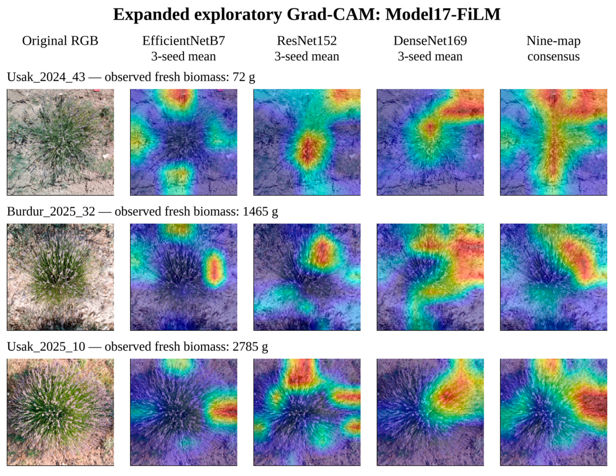
Grad-CAM [43] was evaluated for all 29 locked-test Kok_id units using EfficientNetB7, ResNet152, and DenseNet169 under all three training seeds, yielding 261 maps. One original image per Kok_id was selected deterministically using the lexicographically first filename, without reference to predictions or errors. Each saved Model17-FiLM network retained its original numerical input and training-adapted normalization parameters. Replayed predictions were compared with the corresponding saved image-level predictions using the 5 g tolerance specified in the extraction code. Gradients were computed at the CBAM output according to the regression formulation in Equations (14) and (15):
Here, H and W denote the spatial feature-map dimensions, and αk is the gradient-based weight of channel k. Maps were normalized for each image–model pair and resized to 224 × 224 pixels. Pairwise pixel-wise correlations were calculated across seeds for a fixed backbone and across backbones for a fixed seed. Pixel-wise standard deviations and a nine-map consensus were also computed. Examples for the test units with the minimum, median, and maximum observed biomass are presented in Section 3.12. Map agreement was interpreted as an exploratory stability diagnostic rather than causal biological attribution or a decomposition of the numerical branch.
2.9. Reproducibility, Data, and Code Availability
The fixed Kok_id partition, experimental protocol, prediction outputs, and analysis settings were retained in machine-readable files. Split seed 42 and the combined SHA-256 fingerprint 50e501d587b151f1 977ae16c89763b9f 2cc43a119b36ceab eaf4401b7146bf22 identify the common partition. Training used NVIDIA L4 GPUs with TensorFlow deterministic operations enabled. The principal study findings and revision-stage analyses are presented in the main article. Detailed predictions, analysis summaries, and checksums were retained in the research archive. Access is governed by the Data Availability Statement; the archive has not been presented as a publicly deposited repository.
3. Experimental Results
3.1. Data Audit and Experiment Completion Check
No Kok_id overlapped between the training, validation, and test partitions. All 81 primary model–backbone–seed runs and the 54 additional Model16 and Model17-Concat runs were completed under the same fixed partition fingerprint. Model and ensemble selection used validation data rather than locked-test performance. The original-image metadata audit reported numerical agreement with the relative-altitude records for all 459 images. The test set comprised 18 Burdur-2025, seven Uşak-2024, and four Uşak-2025 units. These constitute 29 evaluation units, not 29 independently sampled acquisition conditions.
3.2. Primary Equal-Weight Ensemble Performance
Table 5 presents locked-test performance for the three primary model groups under each training seed.
Table 5.
Locked-test performance of the primary validation-selected four-backbone ensembles for each training seed.
The ensemble constructed for each model group and seed combination consisted of four backbones selected according to the validation RMSE.
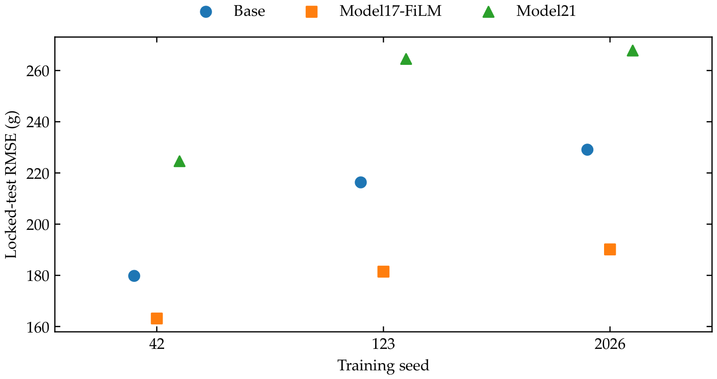
Model17-FiLM achieved lower RMSE and MAE and higher R2 than Base under all three training seeds. For seeds 42/123/2026, RMSE values were 179.8/216.3/229.1 g for Base, 163.2/181.5/190.1 g for Model17-FiLM, and 224.6/264.5/267.8 g for Model21. EfficientNetB7 and EfficientNetB1 were selected for the Model17-FiLM four-backbone ensemble under every seed, whereas the other two members varied. This indicates partial stability of ensemble membership rather than a single invariant composition. In the validation-only post hoc screening of ensemble sizes from two to eight, the lowest validation RMSE occurred at k = 2 in eight of the nine conditions and at k = 3 in one. The prespecified k = 4 solution was retained in all nine conditions. Its validation RMSE was within 5% of the best value across ensemble sizes in seven out of nine conditions and within 10% in all nine conditions. These findings demonstrate sensitivity to the validation sample and ensemble size. Because screening was confined to validation data, the primary k = 4 protocol was not revised on the basis of locked-test performance. Figure 3 shows variation in RMSE across training seeds.
Figure 3.
Locked-test RMSE of the primary validation-selected four-backbone ensembles for Base, Model17-FiLM, and Model21 under three training seeds. Seeds are categorical labels, and all points use the same 29 test Kok_id units. Repeated seeds do not represent independent test datasets.
3.3. Stability of the 81 Individual Models and Backbones
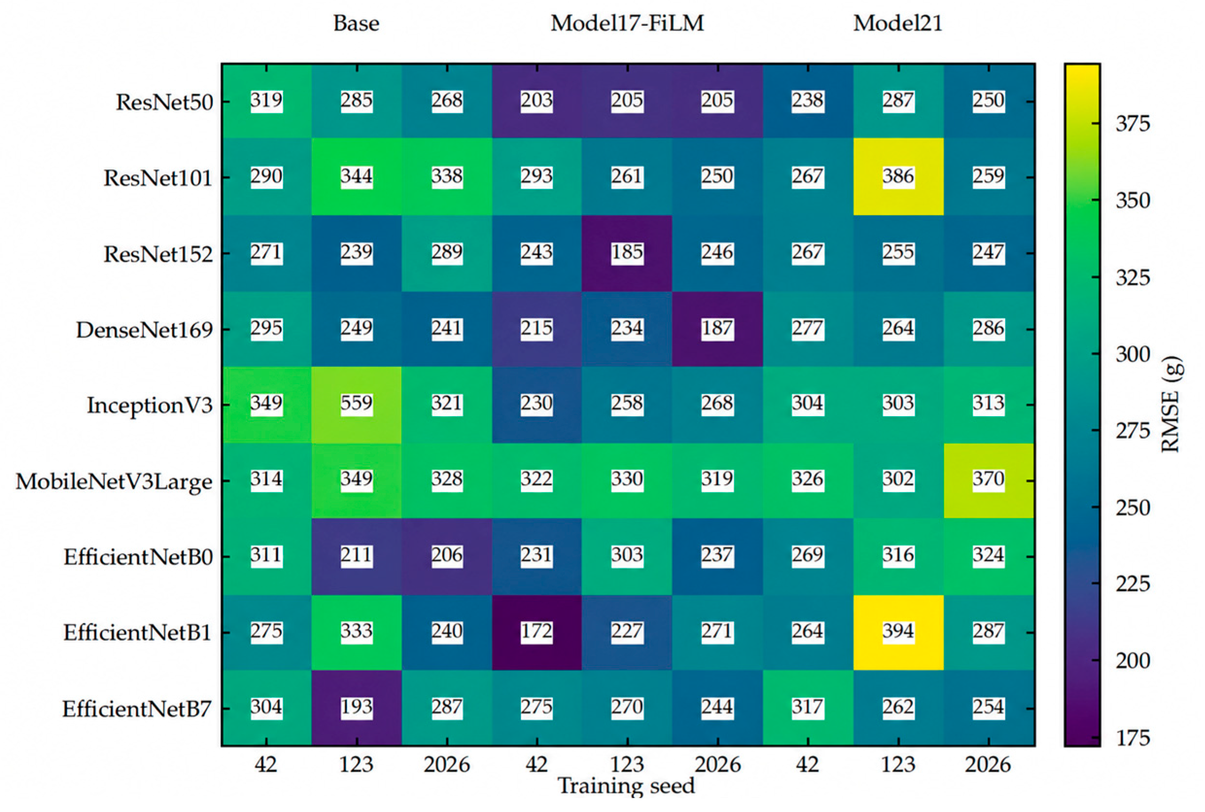
The stability of the individual models across the three seeds demonstrated that the effect of visual–numerical fusion was not dependent solely on a particular ensemble combination. For matched backbone–seed pairs, Model17-FiLM outperformed the Base model in 21 of 27 comparisons for each of the R2, MAE, and RMSE metrics. The number of matched comparisons in which all three metrics improved simultaneously was 19/27. Based on the three-seed averages for each backbone, Model17-FiLM achieved lower RMSE for seven of the nine backbones and lower MAE together with higher R2 for eight of the nine backbones compared with the Base model. The Model17-FiLM ResNet50 network was one of the most stable individual models. It exhibited low across-seed variability, with R2 = 0.9140 ± 0.0011, MAE = 162.3 ± 6.8 g, and RMSE = 204.1 ± 1.3 g. For Model17-FiLM, the three-seed mean RMSE of the primary ensemble model was 178.2 g. This difference is consistent with an improvement in point-estimate performance obtained by averaging the selected backbones. However, it cannot be interpreted as an independent test of superiority over the best individual backbone. The locked-test RMSE values of the 81 individual models obtained across the three model groups, nine backbones, and three seeds are collectively presented in Figure 4.
Figure 4.
Locked-test RMSE for the 81 primary models. Rows represent the nine backbones, and columns represent the three training seeds within each model group. Cell values are RMSE in grams. A single color scale is applied to the complete matrix. The 54 additional control-model runs are not included in this primary-experiment figure.
3.4. Primary Controlled Model-Group Comparison
Table 6 summarizes the mean performance of each primary model group and its variability across the three training seeds.
Table 6.
Performance stability of the primary equal-weight ensemble model across the three seeds.
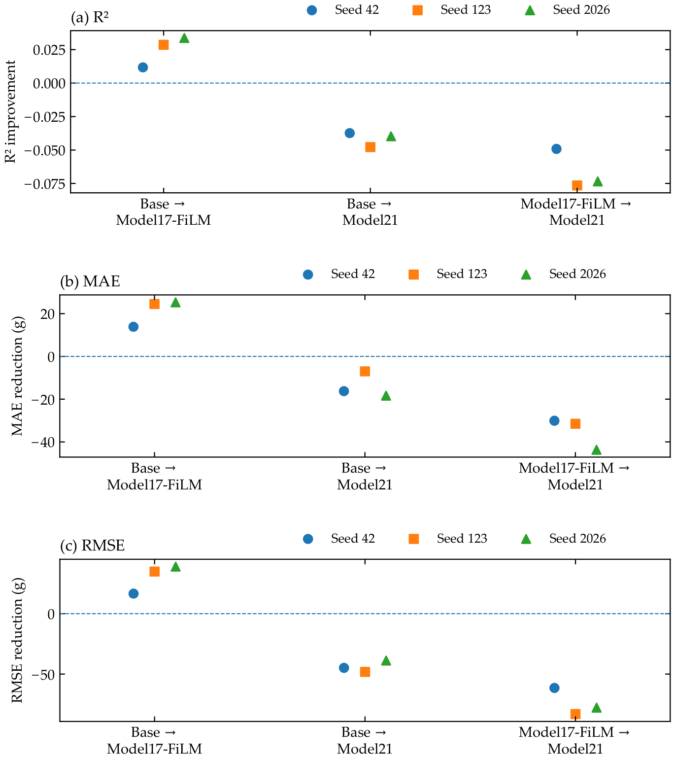
Across the three training seeds, Model17-FiLM reduced mean RMSE by 30.2 g and mean MAE by 21.2 g relative to Base, while increasing mean R2 by 0.0247. The direction of improvement was consistent across all three seeds. Relative to Model17-FiLM, Model21 increased mean RMSE by 74.1 g and mean MAE by 35.1 g and reduced mean R2 by 0.0663. Model21 did not outperform Model17-FiLM under any seed. Model21 also had a higher three-seed mean RMSE than Base (252.3 versus 208.4 g). However, the Base-to-Model21 bootstrap intervals in the across-seed prediction-mean analysis included zero, so this difference was not interpreted as evidence of the statistical superiority of Base. Under the evaluated fixed-partition protocol, the additional scale block did not provide a predictive gain for the validation-selected equal-weight ensemble. Figure 5 shows the direction and magnitude of the primary model-group contrasts across seeds.
Figure 5.
Seed-level effects for the three primary model-group comparisons: (a) change in R2, (b) reduction in MAE (g), and (c) reduction in RMSE (g). Positive values favor the model on the right. R² differences are calculated as right minus left, whereas MAE and RMSE reductions are calculated as left minus right. Markers identify training seeds 42, 123, and 2026. Each panel uses the corresponding metric and units. The horizontal reference line indicates no change.
3.5. Across-Seed Prediction Mean (Seed-Mean) and Paired Inference
Table 7 reports metrics calculated after averaging the three seed-specific predictions for each Kok_id, together with their 95% confidence intervals.
Table 7.
Secondary across-seed prediction mean (seed-mean) analysis was based on the arithmetic mean of predictions from three training runs on the same 29 test Kok_id samples.
For the across-seed prediction mean, Model17-FiLM achieved R2 = 0.9502 (95% CI 0.9083–0.9740), MAE = 116.7 g (81.2–157.4), and RMSE = 155.3 g (111.6–198.5). This result represents the average of the validation-selected ensemble predictions from three separate training runs and is not interpreted as the expected performance of a single run. As shown in Table 8, for Base→Model17-FiLM, the paired bootstrap effect was +0.0316 for R2, 39.5 g for MAE, and 43.3 g for RMSE, with all confidence intervals excluding zero. In the prespecified directional paired permutation tests, the Holm-adjusted p-values were 0.0006 for R2, 0.0180 for MAE, and 0.0030 for RMSE. In the directional Wilcoxon tests based on the absolute and squared errors, the corresponding values were 0.0221 and 0.0053, respectively. In the recalculated post hoc two-sided sensitivity analyses using the same locked predictions, the Holm-adjusted permutation p-values for R2/MAE/RMSE were 0.0030/0.0348/0.0042, whereas the Wilcoxon p-values for absolute/squared errors were 0.0443/0.0105. Although the effect was in the same direction in all three training runs, none of the comparisons in the single-seed Holm analyses crossed the 0.05 threshold for significance. Therefore, the primary interpretation was based on paired effect sizes and confidence intervals. The single-seed results were regarded as indicators of stability, whereas the across-seed prediction mean was treated as a complementary paired inference.
Table 8.
Paired percentile-bootstrap contrasts for the across-seed mean predictions of the primary selected-four ensembles.
In the Model17-FiLM→Model21 comparison, when the bootstrap effects were defined in favor of the model group on the right, they were −0.0726 for R2, −55.5 g for MAE, and −88.3 g for RMSE, with negative 95% confidence intervals. This indicates that Model21 produced more errors than Model17-FiLM. The prespecified one-sided tests under the hypothesis that the model group on the right would perform better were not designed to test this deterioration because the observed effect occurred in the direction opposite to that expected and was not significant after Holm correction. In the post hoc two-sided paired permutation sensitivity tests conducted to evaluate direction-independent evidence, the Holm-adjusted p-values were 0.0464 for R2, 0.0912 for MAE, and 0.04999 for RMSE. The two-sided Wilcoxon tests based on absolute/squared errors were not significant after Holm correction (p = 0.2017 and p = 0.1520). Thus, although the deterioration in Model21 was consistent in terms of bootstrap effect sizes, the evidence based on two-sided tests varied according to the metric. For the Base→Model21 comparison, the Holm-adjusted p-values from the post hoc two-sided permutation tests were 0.4107/0.4861/0.4153 for R2/MAE/RMSE, respectively, and did not support a statistically significant difference between the model groups. The relationship between the Model17-FiLM across-seed prediction mean and the observed values is shown in Figure 6, together with the 1:1 line and the calibration regression.
Figure 6.
Observed versus predicted fresh biomass for the across-seed mean of the primary Model17-FiLM selected-four ensembles (n = 29 Kok_id). Vertical bars show ±1 standard deviation across the three seed predictions and are not prediction intervals. The reference line denotes 1:1 agreement. The prediction-on-observation regression is ŷ = 126.8 + 0.908y.
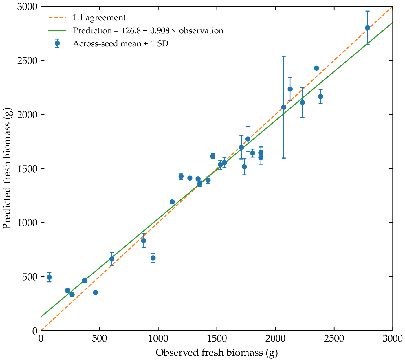
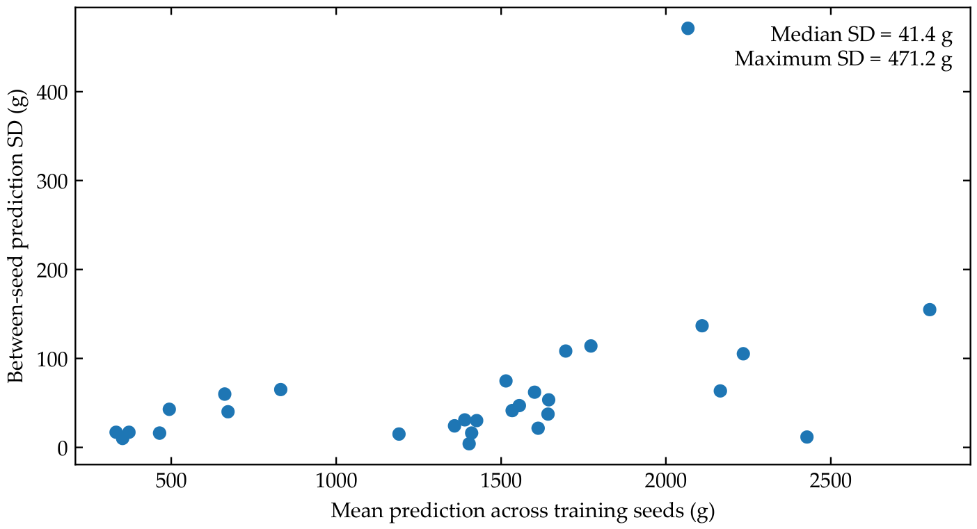
The Model17-FiLM prediction-on-observation calibration slope was 0.9080 (95% bootstrap interval: 0.8194–0.9911), and the intercept was 126.8 g (−14.7 to 264.4 g). Mean bias was −2.7 g. The near-zero mean bias indicates limited average directional deviation, but it does not establish calibration across the target range. The slope below one indicates compression of the predicted dynamic range. No external recalibration recommendation was inferred from this internal analysis. The median between-seed prediction SD per Kok_id was 41.4 g, with a maximum of 471.2 g. Figure 7 shows this variability, which can reflect both stochastic training and seed-specific ensemble composition.
Figure 7.
Between-seed prediction standard deviation for each of the 29 locked-test Kok_id units, plotted against the correspondingmean prediction. Values describe variability across three Model17-FiLM selected-four ensembles and do not quantify the full uncertainty associated with new fields, years, or data partitions.
3.6. Component-Level Ablation: Base → Model16 → Model17-FiLM
Table 9 reports the all-nine ensembles after averaging predictions across the three training seeds for each test Kok_id. Base achieved RMSE = 196.78 g and MAE = 153.47 g. Adding the 16 engineered RGB descriptors through the numerical FiLM branch reduced these to 166.27 and 131.34 g in Model16. Model17-FiLM, which additionally used HasatOncesiGunSayisi, achieved RMSE = 163.32 g and MAE = 130.79 g.
Table 9.
Component-ablation performance calculated after averaging all-nine ensemble predictions across the three training seeds for each of the 29 locked-test Kok_id units.
The Base-to-Model16 improvements were 30.51 g for RMSE (95% bootstrap interval: 1.56–62.36 g), 22.14 g for MAE (0.02–47.61 g), 0.02285 for R2 (0.0013–0.0527), and 0.01375 for CCC (0.0007–0.0306). These pointwise intervals excluded zero, although the MAE lower bound was close to zero. The results support an improvement associated with the engineered-descriptor branch and FiLM relative to Base under the fixed protocol.
The Model16-to-Model17-FiLM improvements were smaller: 2.95 g for RMSE (−7.66 to 11.38 g), 0.55 g for MAE (−7.55 to 7.54 g), 0.00201 for R2 (−0.0063 to 0.0084), and 0.00133 for CCC (−0.0029 to 0.0052). All intervals included zero. Thus, the incremental value of the harvest-timing covariate was uncertain, conditional on the 16-descriptor FiLM model. This is not evidence that phenology is generally uninformative.
3.7. Fusion-Operator Control and Numerical-Only Baseline
For independently validation-selected four-backbone pipelines, FiLM achieved RMSE = 155.34 g, compared with 171.45 g for concatenation, a reduction of 16.12 g or 9.40%. The corresponding MAEs were 116.65 and 130.68 g. In the all-nine analysis, RMSE was 163.32 g for FiLM and 175.81 g for concatenation, a reduction of 12.49 g or 7.10%. Table 10 separates these two ensemble strategies.
Table 10.
FiLM versus concatenation on the same 29 locked-test Kok_id units. Metrics were calculated after averaging predictions across training seeds separately for selected-four and all-nine ensembles.
For selected-four pipelines, the paired-bootstrap RMSE difference favored FiLM by 16.12 g (95% interval: 4.13–31.33 g), whereas the MAE interval included zero (−0.89 to 30.28 g). In the all-nine comparison, the RMSE difference was 12.49 g (0.92–27.74 g), and the MAE interval again included zero (−3.94 to 23.69 g). The Holm-adjusted selected-four permutation p values were 0.0870 for RMSE, 0.0976 for MAE, 0.0870 for R2, and 0.0444 for CCC. The corresponding Wilcoxon values were 0.0870 for both absolute and squared errors. None of the all-nine adjusted tests was below 0.05. Bootstrap intervals and multiplicity-adjusted tests are distinct summaries and did not provide uniform evidence of superiority. The supported conclusion is a FiLM advantage in point estimates within the evaluated protocol.
The validation-selected RF17 baseline achieved locked-test RMSE = 423.52 g, MAE = 269.77 g, R2 = 0.6300, CCC = 0.7859, and bias = −11.12 g. Its validation RMSE was 563.10 g. These results describe this tuned Random Forest baseline, not all possible numerical-only learners. RF17 did not reproduce the accuracy of the evaluated visual–numerical models.
3.8. Persistent-Plant, Scale-Variable, and Field-Year Sensitivity
PersistentID restriction excluded seven of the 29 test units whose site-plus-root identifier had occurred in training or validation, leaving 22 units. For the primary selected-four prediction means, RMSE/R2 were 146.21 g/0.9019 for Model17-FiLM, 158.86 g/0.8842 for Model17-Concat, 176.49 g/0.8571 for Base, and 189.39 g/0.8355 for Model21. The principal RMSE ranking was retained. These restricted-subset metrics should not be interpreted as direct improvements or deteriorations relative to the full-test metrics because the target distribution and evaluation sample changed.
On the 362 original training images, the relative-altitude/GSD-proxy Pearson correlation was 1.000. The correlation between area_gsd_cm2 and perimeter_gsd_cm was 0.848. The relative altitude and its GSD proxy correlated with the metadata-scaled geometry at approximately 0.70–0.74. These descriptive results identify overlapping inputs, but do not establish collinearity as the cause of Model21 performance.
When the equal-weight Model17-FiLM and Model21 ensembles were compared separately across metadata-derived relative altitude and nominal GSD proxy groups, Model17-FiLM exhibited lower RMSE and MAE in the vast majority of the groups. Considering the metadata-derived relative altitude groups alone, Model17-FiLM produced lower errors for both metrics in eight of the nine seed × group conditions. The only exception was the highest metadata-derived relative altitude group for seed 123 (group sample sizes, n = 7–13). However, because of the fixed camera geometry, nominal GSD proxy and metadata-derived relative altitude were perfectly linearly dependent. Therefore, these two groupings were not combined as independent sets of evidence. The number of samples within the groups ranged from 1 to 13, and one of the GSD groups contained only a single Kok_id. Therefore, the results were regarded solely as descriptive sensitivity evidence. Which scale variable was responsible for the change in performance cannot be determined separately using the current block-ablation design.
For the across-seed mean Model17-FiLM results at the field-year level, the Burdur-2025 subgroup had n = 18 and RMSE = 144.3 g, whereas the Uşak-2024 subgroup had n = 7 and RMSE = 209.5 g. The Uşak-2025 subgroup contained only four Kok_id samples and had an RMSE of 67.0 g. In this very small subgroup, variance-based metrics such as R2 were not emphasized as evidence of generalizability. Because field and year were not fully factorial in the current design, their effects could not be disentangled.
These small, imbalanced subgroups do not permit causal attribution of prediction differences to soil, management, plant age, or location.
3.9. Technical-Dependence and Acquisition-Session Audits
In the separate image-level validation-selected pipeline, Base and Model17-FiLM achieved RMSEs of 237.35 and 214.86 g, respectively. Their difference was 22.49 g. The pointwise 95% bootstrap interval was −1.53 to 51.40 g under image resampling, 4.09 to 46.84 g under Kok_id group resampling, and −7.06 to 68.77 g under Ucus_No group resampling. Acquisition-group resampling produced a wider interval that included zero. These results concern the alternative image-level pipeline and are not a replacement for the primary Kok_id-level contrast.
A training-only Ucus_No target-mean baseline achieved R2 = 0.6398, MAE = 379.17 g, and RMSE = 476.15 g across the 46 test images. All 10 test Ucus_No groups were represented in training. Acquisition-group membership therefore carried target-related information, although this baseline did not reach the audited Model17-FiLM accuracy. Ucus_No denotes the operational grouping in the archived records, not a demonstrated set of independent acquisition campaigns.
For seven Uşak-2024 units imaged 13 and 3 days before harvest, Model17-FiLM predictions increased in all seven cases, with a mean difference of +152.22 g. Absolute error improved in three cases and worsened in four. Both image dates were evaluated against the same final-harvest mass. This is a temporal prediction-sensitivity result, not validation of biomass growth trajectories or an isolated timing-covariate effect.
3.10. Field-Marker Context Sensitivity
The detector identified candidate field markers in 15 of 46 test images (32.6%), representing 10 distinct Kok_id units. The analysis was conducted at the image level, not on 15 independent plants. In these images, the mean absolute prediction change was 118.12 g after marker-region occlusion. The mean of the per-image median absolute matched-control changes was 37.89 g. The excess marker effect was 80.24 g (95% paired image-bootstrap interval: 28.92–147.95 g). Mean marker-box Grad-CAM enrichment relative to uniform image-area allocation was 5.33-fold, and marker-minus-control enrichment was 4.59 (1.19–8.55).
Mean change in absolute error after marker occlusion was −30.41 g (−90.18 to 43.02 g), where negative values indicate lower error. The interval included zero. These findings show sensitivity to detector-defined marker regions in the audited seed-123 EfficientNetB1 network. They do not establish an ensemble-wide causal shortcut, and image-level intervals do not account for repeated-plant or acquisition-session dependence.
3.11. Error Distribution and Target Range
No marked increase in error was observed for the highest biomass quartile (Q4) in the locked test partition. When the Model17-FiLM across-seed mean predictions were stratified according to quartiles of the actual biomass values, RMSE was approximately Q1 = 197.0 g, Q2 = 122.6 g, Q3 = 159.3 g, and Q4 = 116.3 g, whereas the bias was +42.3, +88.8, −112.3, and −23.5 g, respectively. Thus, within the locked test range, error did not increase monotonically with biomass. However, whereas the maximum value in the test set was 2785 g, the training target extended up to 4480 g. Therefore, no external validation evidence is available for high biomass values above 2785 g.
3.12. Expanded Multi-Backbone Grad-CAM Stability
The expanded analysis comprised 261 maps from 29 test Kok_id units, three backbones, and three seeds. The mean pixel-wise correlation across seeds for a fixed backbone was 0.3613. The mean correlation across backbones for a fixed seed was 0.0530. The maps therefore showed limited seed-level agreement and much lower cross-backbone agreement. Figure 8 presents three biomass-ranked examples from this complete analysis. Neither the number of maps nor the number of pairwise correlations increase the number of biological test units. The response maps are exploratory and do not identify causal biomass-generating structures or isolate numerical-branch contributions.
Figure 8.
Expanded exploratory Grad-CAM analysis for the test units with the minimum, median, and maximum ob-served fresh biomass: Usak_2024_43 (72 g), Burdur_2025_32 (1465 g), and Usak_2025_10 (2785 g), respectively. Columns show the original RGB image, the three-seed mean Grad-CAM maps for EfficientNetB7, ResNet152, and DenseNet169, and the consensus across the nine backbone–seed maps. Cases were selected by observed-biomass rank rather than prediction error. Colors encode the relative magnitude of the displayed Grad-CAM responses, not biomass values or prediction errors. Individual maps were normalized before averaging. Consequently, color intensity does not represent an absolute effect magnitude comparable across cases or models. These maps are ex-ploratory visual-response summaries and should not be interpreted as causal biological attribu-tions.
4. Discussion
The additional controls clarify the pattern of improvement observed for Model17-FiLM. In the all-nine across-seed prediction-mean analysis, RMSE decreased from 196.78 g for Base to 166.27 g for Model16 and 163.32 g for Model17-FiLM (Table 9). Most of this sequential reduction occurred when the engineered-descriptor branch with FiLM was added. The subsequent timing-covariate increment was small and uncertain. This supports the evaluated descriptor-conditioned representation, but does not isolate each descriptor, establish a timing-only contribution, or demonstrate a full factorial interaction. The estimates remain conditional on one partition and one dataset.
FiLM produced lower point-estimate errors than direct concatenation under both subset-selection strategies (Table 10). The all-nine result is particularly useful because it avoids differences in the four-backbone subsets selected for each architecture. Nevertheless, fused dimensions and parameterization differ between FiLM and concatenation, and adjusted inferential support was not uniform across metrics. RF17 further showed that this particular numerical-only learner did not reproduce the multimodal accuracies. Neither comparison establishes universal superiority of FiLM or deep learning over alternative fusion operators and numerical learners.
Model21 did not improve compared to Model17-FiLM in any primary seed condition. The descriptive correlation analysis supports substantial redundancy within the scale block, including deterministic proportionality between relative altitude and the nominal GSD proxy. The scale inputs also lack direct camera-to-canopy calibration. These properties are plausible contributors to the absence of additional predictive gain, but their causal contributions were not separated. The result should not be generalized to physically calibrated GSD, canopy geometry, or independently measured structural variables.
Studies on visual and numerical context fusion likewise indicate that the benefit of additional data sources is problem-dependent. In studies on rice, soybean, and maize, integrating environmental or phenotypic context with image representations has yielded strong predictions [10,11,12]. In contrast, in a konjac AGB study, the finding that SVR using selected RGB spectral and textural variables outperformed an image-based AlexNet approach indicates that architectural complexity alone does not guarantee superior performance [9]. Through the controlled Base→Model17-FiLM→Model21 sequence implemented under the same visual architecture, the present study demonstrates that the direction of the contribution from additional context may depend on the dataset and the degree of information redundancy.
The ensemble results also emphasize the dependence of selection on the validation sample. Although EfficientNetB7 and EfficientNetB1 were selected for Model17-FiLM equal-weight ensemble under all three seeds, the remaining two components varied. Under each model group–seed condition, screening 126 four-model combinations using only 29 validation Kok_id samples may introduce validation-based selection optimism, even though the locked test set was not used. Indeed, in the post hoc 2–8 model screening conducted using validation data only, the best validation RMSE by ensemble size was obtained with a two-model ensemble in 8/9 conditions and a three-model ensemble in 1/9 conditions. The prespecified and locked four-model solution (k = 4) remained within 10% of the best validation RMSE by ensemble size in all conditions. This finding indicates that the four-model solution is not universally optimal for validation and that the selection is sensitive to the small validation sample. The secondary convex-blending solution collapsing to an EfficientNetB1 weight of 1.0 for Model17-FiLM under all seed conditions also suggests that flexible weight optimization may behave like single-model selection rather than a genuine ensemble. Therefore, the primary four-model equal-weight method was retained as the prespecified and locked architecture. The post hoc screening was interpreted solely as evidence of selection sensitivity without accessing the test data.
All-nine analyses in Section 3.6 and Section 3.7 removed subset screening and retained the favorable point-estimate patterns for descriptor-conditioned models and FiLM. They do not remove validation-based checkpoint selection or uncertainty from the fixed data split.
4.1. Relationship to Other Lavender and Plant Biomass Studies
Bozkurt et al. [3] used 224 RGB images from 64 individual lavender plants in the Uşak Central District. They modeled HSV-based segmentation, GLCM, and volumetric features using Random Forest. The reported independent test performance was R2 = 0.5974, MAE = 171.55 g, and RMSE = 200.97 g. The present study uses an expanded field/year data structure from the same line of research. It differs from the previous study in terms of data coverage, target distribution, field-year structure, primary Kok_id-level sample analysis, and model group. However, because the exact file-level overlap with the previous 224 images was not encoded as a separate field in the current experimental records, the two studies were not treated as independent external datasets and were not considered a direct model comparison. The performance of Model17-FiLM on the current locked partition was interpreted solely as a result of the present experimental design. Without independent validation in a third field/year, it cannot be extended into a claim of superiority or generalizability to broader populations.
The literature indicates that high accuracy is not specific to a single model class. Random Forest for UAS-based shrub willow biomass, ANN for UAV multispectral wheat biomass, PCA-SVR for konjac AGB, and CatBoost for rice AGB have all produced strong results under different combinations of data characteristics, feature extraction procedures, and model matching [9,44,45,46]. Therefore, the R2 and gram-based error values obtained in the present study cannot be converted into a direct ranking of superiority over published studies using different target units and sensors. Because the studies presented in Table 11 used different units and evaluation methods, no direct performance ranking was made among their results.
Table 11.
Selected biomass and yield prediction studies and the position of the present study. Targets, units, and evaluation protocols differ, so rows do not support a direct performance ranking.
4.2. Scale, Generalizability, and Explainability
Qu et al. [16] examined the effects of flight altitude and sampling strategy on UAV-RGB-based wild blueberry yield estimation. Although the scale block of Model21 did not improve performance in the present study, this result should not be generalized to imply that GSD is uninformative. The nominal GSD proxy used here is perfectly linearly dependent on metadata-derived relative altitude and does not represent true orthomosaic/GCP calibration. In addition, the GSD range of the test data is narrower than that of the training data. Stronger inference would require controlled fixed-altitude or calibrated-GSD experiments together with individual ablation of the scale variables.
The expanded Grad-CAM analysis showed limited agreement across seeds and very low agreement across backbones (Section 3.12 and Figure 8). A map therefore describes the response of a particular trained visual network in its numerical context, rather than a unique explanation of the ensemble. Grad-CAM does not separate the numerical branch or establish biological causality.
The marker-occlusion audit identified contextual sensitivity in one backbone–seed model. Larger prediction changes for detected-marker regions than for matched controls warrant attention, but marker removal did not consistently reduce error. Because the intervention kept numerical descriptors fixed, modified-image distribution shift and visual–numerical inconsistency also limit interpretation. Marker masking before training and independent marker-free validation are appropriate subjects for future evaluation, not benefits established by the current audit.
4.3. Limitations and Future Work
The study used one fixed Kok_id-grouped split. Training-seed variation reflects stochastic optimization, not alternative sampling partitions. The 29 test Kok_id units share acquisition groups, and some perennial positions recur across years. The three seeds, 46 images, and 261 Grad-CAM maps are not additional independent biological test replicates. PersistentID restriction preserved the principal ranking but did not replace external field-year validation.
The field-year design was imbalanced, with Burdur represented only in 2025. Image-based eligibility can favor visually separable plants, and sampling was not formally randomized. Image-level acquisition-group resampling in the separate sensitivity pipeline widened uncertainty. All test Ucus_No groups were represented in training, so unseen session performance was not established. The image-level sensitivity pipeline differs from the primary Kok_id-level pipeline and cannot be pooled with it as independent evidence.
Reference mass was measured using a scale with 5 g readability, without calibration against certified reference weights or a systematically recorded replicate-weighing protocol. Empirical weighing uncertainty therefore could not be estimated. The maximum 2 h weighing delay does not establish negligible moisture loss, and no delay-specific mass-loss correction was available. Meteorological descriptors were derived from ERA5-Land rather than plot-level sensors, and terrain slopes were map-based approximations.
Planting spacings describe the sites but were not experimental factors in this analysis. At Uşak, the described layout comprised five rows, with each spacing arrangement occupying one-third of the planted area within every row. However, the analytical records did not establish the row and spacing-section membership of individual sampled Kok_id units, and spacing-specific biomass or prediction errors were not evaluated. Equal planted-area allocation therefore does not demonstrate balanced representation of the spacing classes in the image-eligible sample. Nominal spacing-derived densities do not account for missing plants, boundary effects, or non-planted areas. No per-hectare biomass estimates or hectare-scale error were validated. Decimal-coordinate masking also limits independent reproduction of site-specific meteorological extraction from the published article alone.
HasatOncesiGunSayisi was calculated using the recorded actual harvest date. Prospective application requires a harvest date that is available at prediction time, and substituting a planned date has not been validated. Its incremental contribution remained uncertain in the sequential Model16 comparison, and direct phenological-stage effects were not tested. The Model21 scale block comprised relative-altitude-derived proxies rather than calibrated physical plant dimensions, and the individual effects of its four variables were not isolated.
The marker-occlusion and Grad-CAM analyses were exploratory. Marker occlusion covered one backbone–seed network and detector-defined regions while holding the numerical inputs fixed. Its image-level bootstrap intervals do not account for all potential dependence structures. Neither analysis establishes causal shortcut learning or an ensemble-wide failure.
The maximum test biomass was 2785 g, whereas the training distribution extended to 4480 g. Performance in the upper training tail was therefore not evaluated. Screening 126 subsets on 29 validation units can also produce selection sensitivity. All-nine averaging removes backbone-subset selection but not checkpoint-selection effects or uncertainty associated with the fixed split. Individual checkpoints were selected using image-level MAE, whereas primary ensembles were selected using Kok_id-level RMSE. The revision-stage analyses reused the existing test set after the primary results were available and therefore provide additional internal evidence rather than independent confirmatory validation.
5. Conclusions and Recommendations
The study comprised 135 controlled deep-learning runs across five input/fusion groups, nine backbones, and three training seeds under a fixed Kok_id partition. The primary Model17-FiLM selected-four ensembles achieved R2 = 0.934 ± 0.010 and RMSE = 178.2 ± 13.8 g across seeds. These seed-level metric summaries are distinct from the metrics calculated after averaging predictions across seeds.
In the all-nine across-seed prediction-mean comparison, RMSE decreased from 196.78 g for Base to 166.27 g for Model16 and 163.32 g for Model17-FiLM. Pointwise paired-bootstrap intervals supported the Base-to-Model16 gain, whereas the incremental contribution of harvest timing remained uncertain (Table 9). FiLM produced lower point-estimate errors than concatenation under both ensemble strategies, without uniform multiplicity-adjusted evidence of superiority (Table 10). RF17 did not reproduce the accuracy of the visual–numerical models. The nominal Model21 scale block provided no additional predictive gain and contained substantial redundant information.
Persistent-plant restriction preserved the principal model ranking. Acquisition-session and marker audits identified contextual sensitivity, while the expanded Grad-CAM analysis demonstrated strong backbone dependence. These findings support the evaluated visual–numerical approach within the present dataset rather than broad deployment claims. Independent field-year and acquisition-session validation, more representative sampling, prospectively available timing inputs, and calibrated geometry are required to evaluate the operational transfer.
Author Contributions
Conceptualization: F.D.; methodology: F.D., F.B., M.T.; software: F.B.; validation: F.D., M.T.; formal analysis: F.B.; investigation: F.D., M.T., F.B.; data curation: F.B.; writing—original draft preparation: F.D., M.T., F.B.; writing—review and editing: F.D., M.T.; visualization: F.B.; supervision: F.D., M.T. All authors have read and agreed to the published version of the manuscript.
Funding
This research received no external funding.
Data Availability Statement
The data obtained in this study will be used in planned and ongoing research. It will be made public after the studies are completed and the necessary permissions are obtained.
Acknowledgments
The authors express their gratitude to Ercüment Osman Sarıhan for his voluntary guidance on lavender cultivation and field practices in this study.
Conflicts of Interest
The authors declare no conflicts of interest.
Abbreviations
The following abbreviations are used in this manuscript:
| 3D | Three-Dimensional |
| CNN | Convolutional Neural Network |
| AGB | Above-Ground Biomass |
| ANN | Artificial Neural Network |
| CBAM | Convolutional Block Attention Module |
| CCC | Concordance Correlation Coefficient |
| CI | Confidence Interval |
| CLAHE | Contrast Limited Adaptive Histogram Equalization |
| DEM | Digital Elevation Model |
| DSM | Digital Surface Model |
| DTM | Digital Terrain Model |
| FiLM | Feature-wise Linear Modulation |
| GCP | Ground Control Point |
| GeM | Generalized Mean Pooling |
| GLCM | Gray-Level Co-occurrence Matrix |
| GPU | Graphics Processing Unit |
| GSD | Ground Sampling Distance |
| HSV | Hue, Saturation, Value |
| CIELAB | CIE L*a*b* color space |
| MAE | Mean Absolute Error |
| NIR | Near-Infrared |
| nRMSE | Normalized Root Mean Square Error |
| PCA | Principal Component Analysis |
| RF | Random Forest |
| ReLU | Rectified Linear Unit |
| RGB | Red, Green, Blue |
| RGB-D | Red, Green, Blue–Depth |
| RMSE | Root Mean Square Error |
| SD | Standard Deviation |
| SHA-256 | Secure Hash Algorithm 256-bit |
| SHAP | SHapley Additive exPlanations |
| SVM | Support Vector Machine |
| SVR | Support Vector Regression |
| TF | Texture Features |
| UAS | Unmanned Aircraft System |
| UAV | Unmanned Aerial Vehicle |
| VI | Vegetation Indices |
References
- Pokajewicz, K.; Czarniecka-Wiera, M.; Krajewska, A.; Maciejczyk, E.; Wieczorek, P.P. Lavandula × intermedia A bastard lavender or a plant of many values? Part I. Biology and chemical composition of lavandin. Molecules 2023, 28, 2943. [Google Scholar] [CrossRef] [Scilit]
- Rodríguez-Álvarez, J.L.; García-Alcaraz, J.L.; Puig i Vidal, R.; Cuevas-Jacques, R.; Díaz-Reza, J.R. Noninvasive system for weight estimation in cactus crops: A YOLOv5-decision tree approach based on interval type-2 fuzzy sets. Chemom. Intell. Lab. Syst. 2024, 245, 105064. [Google Scholar] [CrossRef] [Scilit]
- Bozkurt, F.; Teke, M.; Duran, F. Fresh biomass estimation of lavender (Lavandula spp.) using UAV-based RGB imagery, volumetric features and Random Forest regression. Int. J. Eng. Res. Dev. 2026, 18, 80–94. [Google Scholar] [CrossRef] [Scilit]
- Li, B.; Xu, X.; Han, J.; Zhang, L.; Bian, C.; Jin, L.; Liu, J. The estimation of crop emergence in potatoes by UAV RGB imagery. Plant Methods 2019, 15, 15. [Google Scholar] [CrossRef] [Scilit]
- Buxbaum, N.; Lieth, J.H.; Earles, M. Non-destructive plant biomass monitoring with high spatio-temporal resolution via proximal RGB-D imagery and end-to-end deep learning. Front. Plant Sci. 2022, 13, 758818. [Google Scholar] [CrossRef] [Scilit]
- Fei, S.; Hassan, M.A.; Xiao, Y.; Su, X.; Chen, Z.; Cheng, Q.; Duan, F.; Chen, R.; Ma, Y. UAV-based multi-sensor data fusion and machine learning algorithm for yield prediction in wheat. Precis. Agric. 2023, 24, 187–212. [Google Scholar] [CrossRef] [Scilit]
- Yu, D.; Zha, Y.; Sun, Z.; Li, J.; Jin, X.; Zhu, W.; Bian, J.; Ma, L.; Zeng, Y.; Su, Z. Deep convolutional neural networks for estimating maize above-ground biomass using multi-source UAV images: A comparison with traditional machine learning algorithms. Precis. Agric. 2023, 24, 92–113. [Google Scholar] [CrossRef] [Scilit]
- Bhadra, S.; Sagan, V.; Skobalski, J.; Grignola, F.; Sarkar, S.; Vilbig, J. End-to-end 3D CNN for plot-scale soybean yield prediction using multitemporal UAV-based RGB images. Precis. Agric. 2024, 25, 834–864. [Google Scholar] [CrossRef] [Scilit]
- Yang, Z.; Qi, H.; Hu, K.; Kou, W.; Xu, W.; Wang, H.; Lu, N. Estimation of Amorphophallus konjac above-ground biomass by integrating spectral and texture information from unmanned aerial vehicle-based RGB images. Drones 2025, 9, 220. [Google Scholar] [CrossRef] [Scilit]
- Aslam, A.; Farhan, S. Enhancing rice yield prediction: A deep fusion model integrating ResNet50-LSTM with multi-source data. PeerJ Comput. Sci. 2024, 10, e2219. [Google Scholar] [CrossRef] [Scilit]
- Fathi, M.; Shah-Hosseini, R.; Moghimi, A. 3D-ResNet-BiLSTM model: A deep learning model for county-level soybean yield prediction with time-series Sentinel-1, Sentinel-2 imagery, and Daymet data. Remote Sens. 2023, 15, 5551. [Google Scholar] [CrossRef] [Scilit]
- Shamsuddin, D.; Danilevicz, M.F.; Al-Mamun, H.A.; Bennamoun, M.; Edwards, D. Multimodal deep learning integration of image, weather, and phenotypic data under temporal effects for early prediction of maize yield. Remote Sens. 2024, 16, 4043. [Google Scholar] [CrossRef] [Scilit]
- Peng, J.; Wang, D.; Zhu, W.; Yang, T.; Liu, Z.; Rezaei, E.E.; Li, J.; Sun, Z.; Xin, X. Combination of UAV and deep learning to estimate wheat yield at ripening stage: The potential of phenotypic features. Int. J. Appl. Earth Obs. Geoinf. 2023, 124, 103494. [Google Scholar] [CrossRef] [Scilit]
- Sun, C.; Zhang, W.; Zhao, G.; Wu, Q.; Liang, W.; Ren, N.; Cao, H.; Zou, L. Mapping rapeseed (Brassica napus L.) aboveground biomass in different periods using optical and phenotypic metrics derived from UAV hyperspectral and RGB imagery. Front. Plant Sci. 2024, 15, 1504119. [Google Scholar] [CrossRef] [Scilit]
- Togninalli, M.; Wang, X.; Kucera, T.; Shrestha, S.; Juliana, P.; Mondal, S.; Pinto, F.; Govindan, V.; Crespo-Herrera, L.; Huerta-Espino, J.; et al. Multi-modal deep learning improves grain yield prediction in wheat breeding by fusing genomics and phenomics. Bioinformatics 2023, 39, btad336. [Google Scholar] [CrossRef] [Scilit]
- Qu, H.; Zheng, C.; Ji, H.; Barai, K.; Zhang, Y.-J. A fast and efficient approach to estimate wild blueberry yield using machine learning with drone photography: Flight altitude, sampling method and model effects. Comput. Electron. Agric. 2024, 216, 108543. [Google Scholar] [CrossRef] [Scilit]
- Republic of Türkiye, Ministry of Environment, Urbanization and Climate Change, General Directorate of Geographic Information Systems. Türkiye Ulusal Coğrafi Bilgi Sistemi (TUCBS). Available online: https://tucbs.gov.tr/ (accessed on 15 September 2026).
- Muñoz-Sabater, J.; Dutra, E.; Agustí-Panareda, A.; Albergel, C.; Arduini, G.; Balsamo, G.; Boussetta, S.; Choulga, M.; Harrigan, S.; Hersbach, H.; et al. ERA5-Land: A state-of-the-art global reanalysis dataset for land applications. Earth Syst. Sci. Data 2021, 13, 4349–4383. [Google Scholar] [CrossRef] [Scilit]
- Copernicus Climate Change Service (C3S). ERA5 Land Hourly Time-Series Data from 1950 to Present. Climate Data Store. 2025. Available online: https://doi.org/10.24381/ee82e357 (accessed on 15 September 2026). [CrossRef]
- Shorten, C.; Khoshgoftaar, T.M. A survey on image data augmentation for deep learning. J. Big Data 2019, 6, 60. [Google Scholar] [CrossRef] [Scilit]
- Zhang, J.; Tian, H.; Wang, P.; Tansey, K.; Zhang, S.; Li, H. Improving wheat yield estimates using data augmentation models and remotely sensed biophysical indices within deep neural networks in the Guanzhong Plain, PR China. Comput. Electron. Agric. 2022, 192, 106616. [Google Scholar] [CrossRef] [Scilit]
- Zuiderveld, K. Contrast limited adaptive histogram equalization. In Graphics Gems IV; Heckbert, P.S., Ed.; Academic Press: Cambridge, MA, USA, 1994; pp. 474–485. [Google Scholar] [CrossRef] [Scilit]
- Haralick, R.M.; Shanmugam, K.; Dinstein, I. Textural features for image classification. IEEE Trans. Syst. Man Cybern. 1973, SMC-3, 610–621. [Google Scholar] [CrossRef] [Scilit]
- Abbas, S.; Yeniad, M.; Rahebi, J. Alzheimer’s Disease Prediction Using Fisher Mantis Optimization and Hybrid Deep Learning Models. Diagnostics 2025, 15, 1449. [Google Scholar] [CrossRef] [Scilit]
- Szegedy, C.; Vanhoucke, V.; Ioffe, S.; Shlens, J.; Wojna, Z. Rethinking the Inception architecture for computer vision. In Proceedings of the 2016 IEEE Conference on Computer Vision and Pattern Recognition (CVPR), Las Vegas, NV, USA, 27–30 June 2016; pp. 2818–2826. [Google Scholar] [CrossRef] [Scilit]
- Deng, J.; Dong, W.; Socher, R.; Li, L.-J.; Li, K.; Fei-Fei, L. ImageNet: A large-scale hierarchical image database. In Proceedings of the 2009 IEEE Conference on Computer Vision and Pattern Recognition, Miami, FL, USA, 20–25 June 2009; pp. 248–255. [Google Scholar] [CrossRef] [Scilit]
- He, K.; Zhang, X.; Ren, S.; Sun, J. Deep residual learning for image recognition. In Proceedings of the 2016 IEEE Conference on Computer Vision and Pattern Recognition (CVPR), Las Vegas, NV, USA, 27–30 June 2016; pp. 770–778. [Google Scholar] [CrossRef] [Scilit]
- Howard, A.; Sandler, M.; Chu, G.; Chen, L.-C.; Chen, B.; Tan, M.; Wang, W.; Zhu, Y.; Pang, R.; Vasudevan, V.; et al. Searching for MobileNetV3. In Proceedings of the IEEE/CVF International Conference on Computer Vision (ICCV), Seoul, Republic of Korea, 27 October 2019–2 November 2019; pp. 1314–1324. [Google Scholar] [CrossRef] [Scilit]
- Huang, G.; Liu, Z.; van der Maaten, L.; Weinberger, K.Q. Densely connected convolutional networks. In Proceedings of the 2017 IEEE Conference on Computer Vision and Pattern Recognition (CVPR), Honolulu, HI, USA, 21–26 July 2017; pp. 2261–2269. [Google Scholar] [CrossRef] [Scilit]
- Tan, M.; Le, Q.V. EfficientNet: Rethinking model scaling for convolutional neural networks. In Proceedings of the 36th International Conference on Machine Learning, Long Beach, California, USA, 9–15 June 2019; Volume 97, pp. 6105–6114. [Google Scholar]
- Radenović, F.; Tolias, G.; Chum, O. Fine-tuning CNN image retrieval with no human annotation. IEEE Trans. Pattern Anal. Mach. Intell. 2019, 41, 1655–1668. [Google Scholar] [CrossRef] [Scilit]
- Srivastava, N.; Hinton, G.; Krizhevsky, A.; Sutskever, I.; Salakhutdinov, R. Dropout: A simple way to prevent neural networks from overfitting. J. Mach. Learn. Res. 2014, 15, 1929–1958. [Google Scholar]
- Woo, S.; Park, J.; Lee, J.-Y.; Kweon, I.S. CBAM: Convolutional Block Attention Module. In Computer Vision—ECCV 2018; Ferrari, V., Hebert, M., Sminchisescu, C., Weiss, Y., Eds.; Springer: Berlin/Heidelberg, Germany, 2018; pp. 3–19. [Google Scholar] [CrossRef] [Scilit]
- Ba, J.L.; Kiros, J.R.; Hinton, G.E. Layer normalization. arXiv 2016. [Google Scholar] [CrossRef] [Scilit]
- Perez, E.; Strub, F.; de Vries, H.; Dumoulin, V.; Courville, A. FiLM: Visual reasoning with a general conditioning layer. Proc. AAAI Conf. Artif. Intell. 2018, 32. [Google Scholar] [CrossRef] [Scilit]
- Kingma, D.P.; Ba, J. Adam: A method for stochastic optimization. In Proceedings of the 3rd International Conference on Learning Representations (ICLR 2015), San Diego, CA, USA, 7–9 May 2015. [Google Scholar]
- Ioffe, S.; Szegedy, C. Batch normalization: Accelerating deep network training by reducing internal covariate shift. In Proceedings of the 32nd International Conference on Machine Learning; Bach, F., Blei, D., Eds.; PMLR: Online Source, 2015; Volume 37, pp. 448–456. [Google Scholar]
- Huber, P.J. Robust estimation of a location parameter. Ann. Math. Stat. 1964, 35, 73–101. [Google Scholar] [CrossRef] [Scilit]
- Lin, L.I.-K. A concordance correlation coefficient to evaluate reproducibility. Biometrics 1989, 45, 255–268. [Google Scholar] [CrossRef] [Scilit]
- Efron, B.; Tibshirani, R.J. An Introduction to the Bootstrap; Chapman and Hall: New York, NY, USA, 1993. [Google Scholar]
- Wilcoxon, F. Individual comparisons by ranking methods. Biom. Bull. 1945, 1, 80–83. [Google Scholar] [CrossRef] [Scilit]
- Holm, S. A simple sequentially rejective multiple test procedure. Scand. J. Stat. 1979, 6, 65–70. [Google Scholar]
- Selvaraju, R.R.; Cogswell, M.; Das, A.; Vedantam, R.; Parikh, D.; Batra, D. Grad-CAM: Visual explanations from deep networks via gradient-based localization. In Proceedings of the 2017 IEEE International Conference on Computer Vision (ICCV), Venice, Italy, 22–29 October 2017; pp. 618–626. [Google Scholar] [CrossRef] [Scilit]
- Tamiminia, H.; Salehi, B.; Mahdianpari, M.; Beier, C.M.; Klimkowski, D.J.; Volk, T.A. Comparison of machine and deep learning methods to estimate shrub willow biomass from UAS imagery. Can. J. Remote Sens. 2021, 47, 209–227. [Google Scholar] [CrossRef] [Scilit]
- Amorim, J.G.A.; Schreiber, L.V.; de Souza, M.R.Q.; Negreiros, M.; Susin, A.; Bredemeier, C.; Trentin, C.; Vian, A.L.; Andrades-Filho, C.d.O.; Doering, D.; et al. Biomass estimation of spring wheat with machine learning methods using UAV-based multispectral imaging. Int. J. Remote Sens. 2022, 43, 4758–4773. [Google Scholar] [CrossRef] [Scilit]
- Liu, J.; Zhu, X.; Wang, W.; Li, J.; Mustafa, G.; Wang, W.; Chen, Y.; Li, X. Improving accuracy and interpretability of rice aboveground biomass estimation by integrating CatBoost and SHAP model. Food Energy Secur. 2025, 14, e70159. [Google Scholar] [CrossRef] [Scilit]
- Reisi Gahrouei, O.; McNairn, H.; Hosseini, M.; Homayouni, S. Estimation of crop biomass and leaf area index from multitemporal and multispectral imagery using machine learning approaches. Can. J. Remote Sens. 2020, 46, 84–99. [Google Scholar] [CrossRef] [Scilit]
- Aebischer, P.; Sutter, M.; Birkinshaw, A.; Nussbaum, M.; Reidy, B. Herbage biomass predictions from UAV data using a derived digital terrain model and machine learning. Grass Forage Sci. 2024, 79, 530–542. [Google Scholar] [CrossRef] [Scilit]
- Felipetto, H.d.S.; Mercante, E.; Viana, O.; Elias, A.R.; Benin, G.; Scolari, L.; Armadori, A.; Donato, D.G. Combining machine learning with UAV-derived multispectral aerial images for wheat yield prediction in southern Brazil. Eur. J. Remote Sens. 2025, 58, 2464663. [Google Scholar] [CrossRef] [Scilit]
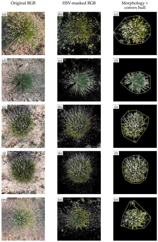
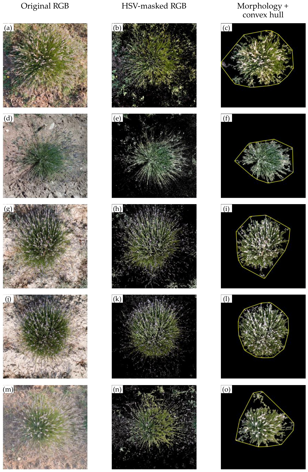
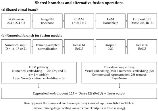
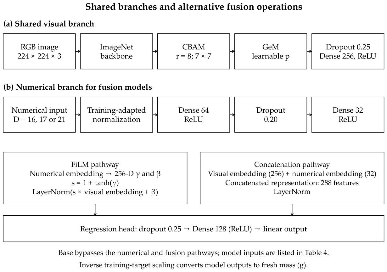

Disclaimer/Publisher’s Note: The statements, opinions and data contained in all publications are solely those of the individual author(s) and contributor(s) and not of MDPI and/or the editor(s). MDPI and/or the editor(s) disclaim responsibility for any injury to people or property resulting from any ideas, methods, instructions or products referred to in the content. |
© 2026 by the authors. Licensee MDPI, Basel, Switzerland. This article is an open access article distributed under the terms and conditions of the Creative Commons Attribution (CC BY) license.