


Abstract
Accurate and efficient estimation of leaf chlorophyll content (LCC) is essential for crop physiological monitoring and precision agriculture. Current remote sensing approaches for LCC estimation mainly rely on machine learning and deep learning methods, which exhibit strong nonlinear modelling capabilities but require sufficient and representative samples. Radiative transfer models (RTMs) can simulate canopy spectral response based on physical mechanisms and generate large-scale datasets, thereby overcoming the limitations of purely data-driven approaches. However, their applications under diverse environmental conditions remain challenging due to uncertainties caused by model parameterization and discrepancies between simulated and observed data. This study proposed a hybrid framework, PROSAIL-DNN-TL, integrating the PROSAIL RTM with full-network fine-tuned transfer learning for winter wheat LCC estimation. First, 85,680 simulated samples generated by PROSAIL were used to pre-train a deep neural network (DNN), and field observations (n = 270) were subsequently used for full-network fine-tuning. A conventional DNN model trained only with field data and machine learning models based on different feature selection strategies were established for comparison. The results showed that: (1) UVE-selected bands were distributed across visible, red-edge, and near-infrared regions; CARS retained more bands in the visible region, whereas SPA mainly selected near-infrared bands; (2) RR and SVR achieved higher accuracy than KNN, with the full-spectrum and CARS feature sets showing superior performance and SPA showing the lowest accuracy; (3) PROSAIL-DNN-TL achieved reliable LCC estimation performance, with an average test R2 of 0.79 across 500 repeated experiments, and showed improved performance compared with conventional machine learning models; (4) PROSAIL-DNN-TL achieved reliable predictive performance when evaluated using datasets collected during the 2024 and 2025 growing seasons, with R2 values of 0.75 and 0.92, respectively. Overall, the proposed hybrid framework integrates physical knowledge from RTMs with data-driven modelling through transfer learning, providing a potential approach for crop chlorophyll monitoring. However, the SPAD-to-LCC conversion used in this study was not specifically calibrated for the instrument and crop, and therefore, the absolute LCC values should be interpreted with caution.
1. Introduction
LCC is a key indicator of a crop’s photosynthetic capacity and nitrogen nutritional status; its accurate estimation is of great significance for crop monitoring [1]. Traditional methods for determining LCC rely primarily on destructive sampling and laboratory chemical analysis; these processes are cumbersome, relatively costly, and make it difficult to carry out large-scale, continuous dynamic monitoring [2]. Advances in remote sensing technology have provided a viable approach for the rapid and non-destructive monitoring of LCC. By analysing the spectral response characteristics of the crop canopy, quantitative monitoring of LCC can be achieved, providing an efficient means of acquiring agricultural information [3]. Hyperspectral remote sensing technology, with its high spectral resolution and detailed data, is capable of capturing various spectral characteristics to identify sensitive bands closely related to crops, thereby enabling precise and efficient monitoring of spectral changes in crops [4,5], and has become the core technical approach for non-destructive LCC monitoring.
Currently, remote sensing-based crop LCC monitoring mainly relies on empirical models, physical models, and hybrid models. Empirical models establish relationships between LCC and spectral characteristics using statistical approaches [6], but their performance is highly dependent on the quality and representativeness of the datasets and can be affected by environmental factors such as soil background and canopy structure [7], resulting in limited robustness and transferability [8]. Physical models describe radiation-canopy interactions based on radiative transfer mechanisms and provide better physical interpretability with reduced dependence on specific regions and crop varieties [9]. However, their application is constrained by complex inversion processes, ill-posed problems, and the requirement for extensive simulations in high-dimensional parameter spaces [3].
Hybrid models combine the advantages of physical and empirical approaches by generating large simulated datasets using RTMs and constructing prediction models through machine learning algorithms [10]. Such models have the potential to reduce dependence on extensive field observations while maintaining physical interpretability and modelling efficiency. Therefore, RTM-based hybrid approaches have been increasingly applied in crop monitoring, including the estimation of biochemical and structural parameters [11]. However, discrepancies between simulated and observed datasets remain a major challenge under diverse environmental conditions, which may reduce model applicability.
Machine learning (ML) methods have been widely used for hyperspectral-based LCC estimation due to their strong nonlinear modelling capabilities [12]. However, conventional ML models generally assume that training and testing datasets share similar feature spaces and distributions; when this assumption is violated, model performance may decline significantly [13]. Traditional ML techniques are unable to process raw data efficiently and require meticulous engineering design and extensive specialist knowledge [14]. In practical applications, differences in crop varieties, growth conditions, environmental factors, and measurement years often result in distribution shifts between training and application scenarios. Consequently, ML models trained on specific datasets may show reduced performance when applied to datasets with different characteristics.
Deep learning (DL) methods can automatically extract hierarchical features from complex datasets and have demonstrated strong performance in remote sensing applications [15,16,17]. DNNs, as representative DL architectures, are capable of modelling complex nonlinear relationships and extracting high-level spectral features [18,19]. However, DNN models typically require large amounts of representative training data and considerable computational resources. Moreover, their black-box characteristics limit model interpretability, and models trained under specific conditions may suffer from overfitting and reduced performance when applied to datasets with different characteristics [20,21,22,23,24,25,26]. These limitations restrict the direct application of conventional ML and DL methods for large-scale and long-term crop monitoring.
Transfer learning (TL) provides an effective strategy for addressing these limitations by transferring knowledge learned from a related source domain to improve model performance in a target domain [27,28,29,30]. By utilizing existing knowledge from source datasets, TL reduces the dependence on large target-domain datasets and decreases computational costs during model training [31]. It is particularly suitable for scenarios where field observations are limited [32]. Therefore, integrating TL with RTMs provides a potential solution for LCC estimation by using simulated data for model pre-training and field observations for fine-tuning, thereby combining the physical knowledge of RTMs with the learning capability of data-driven models.
In summary, although RTM-based hybrid models, ML, and DL methods have been applied in crop parameter estimation, the performance differences among conventional ML, DNN, and TL-based models for winter wheat LCC monitoring remain unclear. Furthermore, the effects of combining multiple feature selection strategies, different feature sets, and PROSAIL-based pre-training have not been systematically investigated.
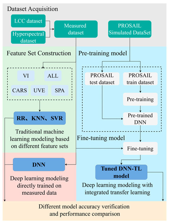
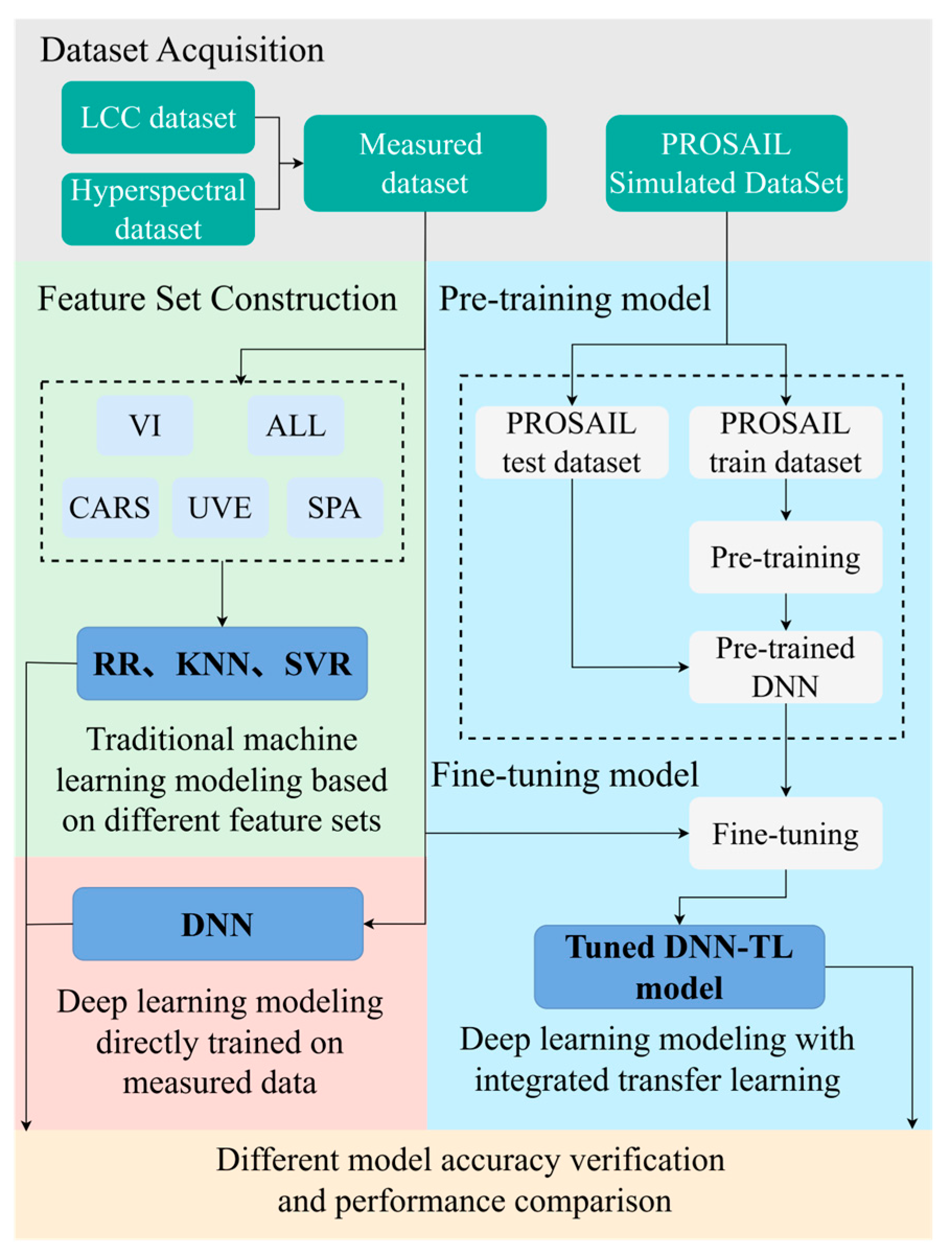
Consequently, this study developed a hybrid model, PROSAIL-DNN-TL, with the following objectives: (1) to develop a transfer learning framework for winter wheat LCC monitoring by integrating ground-based hyperspectral observations with PROSAIL simulations; (2) to compare the performance of traditional ML models based on different feature selection strategies, a conventional DNN model, and the proposed PROSAIL-DNN-TL model; (3) to evaluate the robustness of the proposed model using field datasets collected during two growing seasons. The flowchart of this study is presented in Figure 1.
Figure 1.
Overall framework of the proposed LCC estimation approach based on PROSAIL simulation and transfer learning. The framework includes PROSAIL-based synthetic dataset generation, DNN pre-training using simulated samples, model fine-tuning with measured field data, and comparative evaluation with machine learning models based on different feature selection methods.
2. Materials and Methods
2.1. Study Area
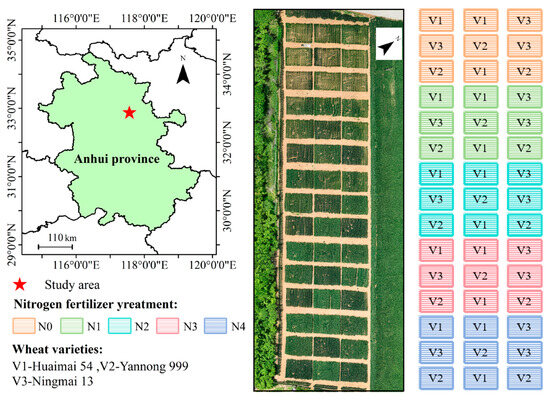
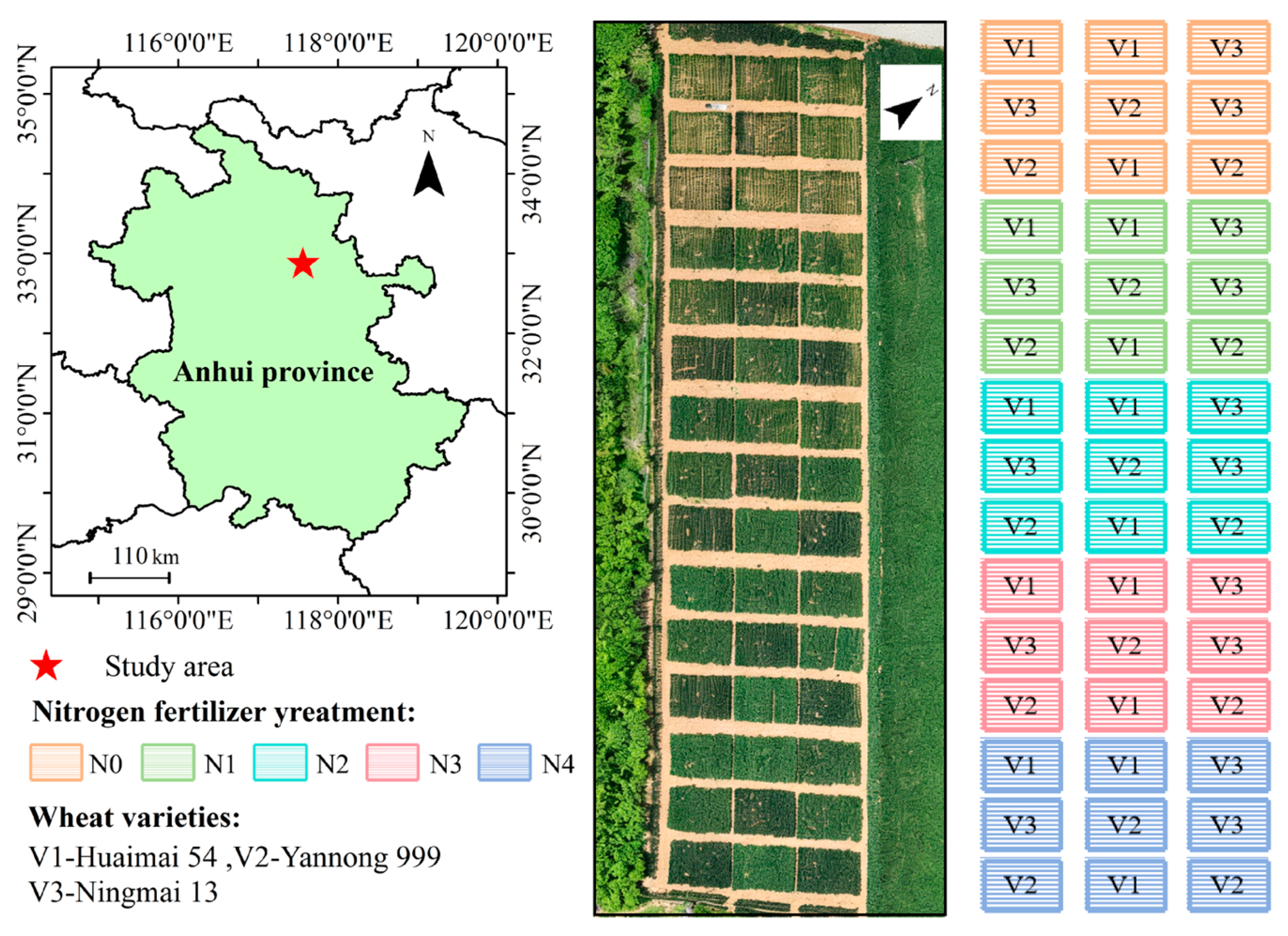
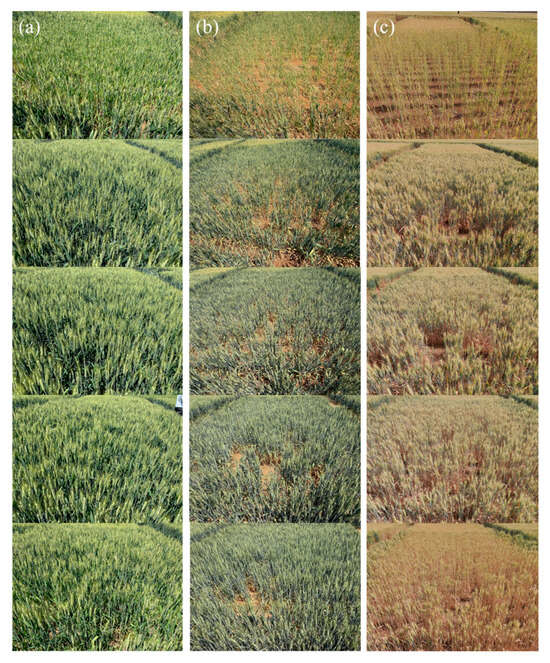
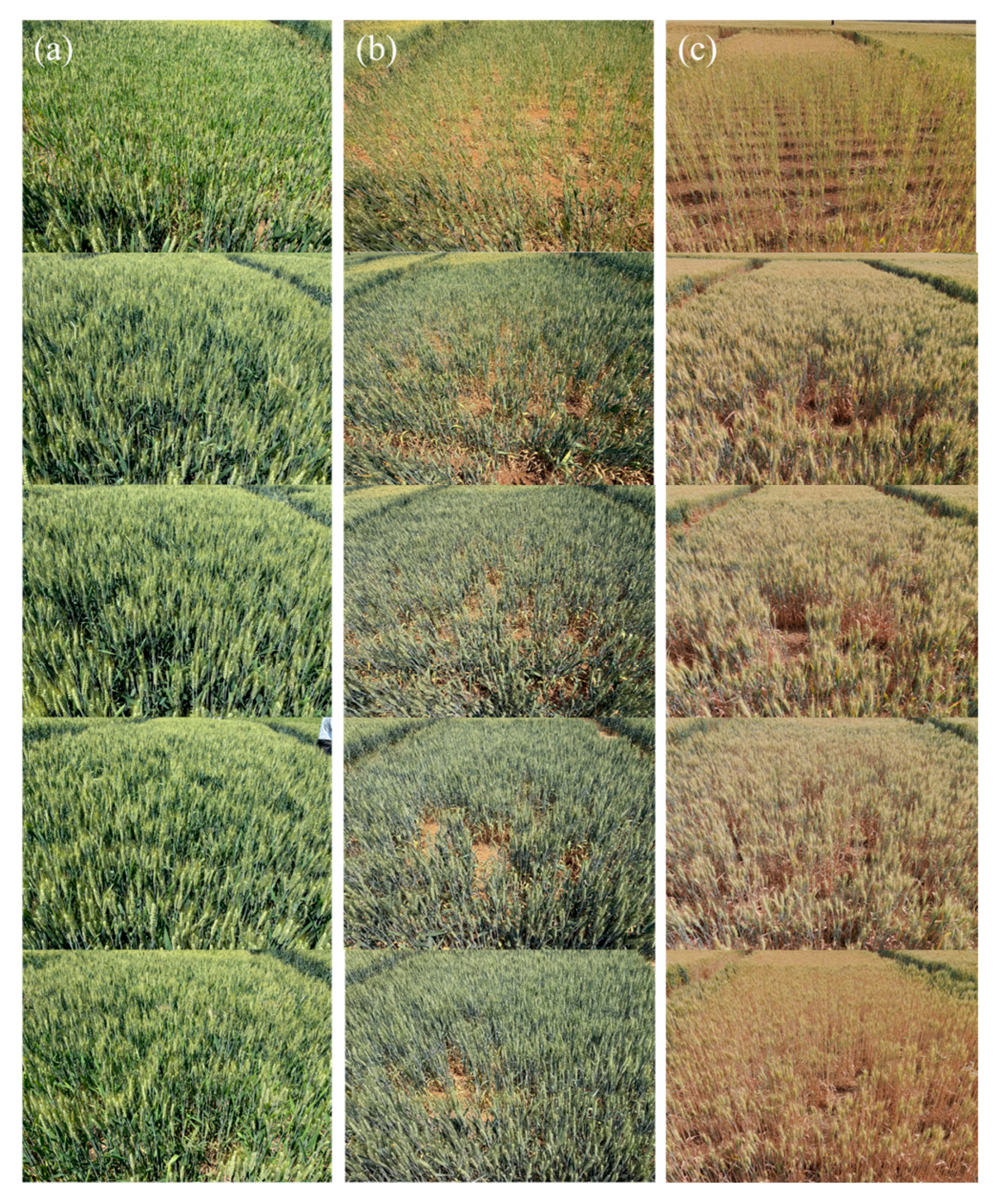
The field experiment was conducted on winter wheat in Shanhou Village, Fengyang County, Chuzhou City, Anhui Province (32°53′15″ N, 117°33′52″ E) (Figure 2). The study area is characterised by a subtropical monsoon climate, with an average annual temperature of 16.3 °C and annual precipitation of 904.7 mm (Anhui Statistical Yearbook, https://tjj.ah.gov.cn/ssah/qwfbjd/tjnj/index.html (accessed on 12 March 2026)). The experiment was conducted during the 2023–2024 and 2024–2025 winter wheat growing seasons. Winter wheat was sown on 25 October 2023 and 30 October 2024, respectively. During the growing seasons, crop development was monitored approximately every two weeks, and field measurements were conducted when winter wheat reached the target phenological stages. Hyperspectral and LCC measurements were collected at three growth stages (Figure 3): jointing stage (16 March 2024 and 18 March 2025), heading stage (18 April 2024 and 19 April 2025), and grain-filling stage (7 May 2024 and 27 April 2025), resulting in six sampling campaigns. A field experiment was designed with five nitrogen application levels, three winter wheat varieties, and three replicates, resulting in a total of 45 experimental plots. The three winter wheat varieties included Huaimai 54 (V1), Yannong 999 (V2), and Ningmai 13 (V3). Nitrogen treatments included N0 (0 kg ha−1), N1 (90 kg ha−1), N2 (180 kg ha−1), N3 (270 kg ha−1), and N4 (360 kg ha−1). Each plot measured 6 m × 4.4 m, with a row spacing of 30 cm, and wheat was sown using a row-seeding method. All experimental plots were located within the same field and shared consistent soil conditions to minimize the influence of soil background differences on spectral measurements.
Figure 2.
Location and experimental design of the study area. The left panel shows the geographic location of the study area in Fengyang County, Anhui Province, China, including the experimental design of nitrogen treatments and winter wheat varieties. The middle panel shows a Field photograph of the experimental area. The right panel shows the Spatial distribution of nitrogen treatments and winter wheat varieties within the experimental plots.
Figure 3.
Real photos of winter wheat at different growth stages, where (a) is the grain filling stage on 7 May 2024, (b) is the grain filling stage on 27 April 2025, and (c) is the maturity stage on 7 May 2025. Each row represents sample plots with different nitrogen gradients from N0 to N4.
2.2. Data Collection
2.2.1. SPAD Data Collection
The relative chlorophyll content (SPAD) of canopy leaves at each growth stage was measured using a TYS-4N plant nutrition analyser (Zhejiang Topyun Agricultural Technology Co., Ltd., Hangzhou, China). Ten winter wheat plants of uniform growth were selected from each plot; measurements were taken at the midpoint of the second leaf of each plant, and the average of the ten samples was taken as the SPAD value for that plot.
Since SPAD measurements provide an indirect estimation of chlorophyll content rather than a direct measurement of leaf chlorophyll concentration, the SPAD values were converted into LCC (μg/cm2) using the empirical relationship proposed by Cerovic et al. [33] (Equation (1)). Although this conversion has been widely adopted for estimating chlorophyll concentration from SPAD measurements, differences in crop species, leaf anatomical characteristics and instrument spectral responses may introduce uncertainty into the absolute LCC values. Therefore, the converted LCC values in this study should be considered as reference estimates rather than direct biochemical measurements. These converted LCC estimates were consistently used as surrogate target variables for model training and evaluation. The detailed LCC values are presented in Table 1.
LCC = (90 × SPAD)/(144 − SPAD)
Table 1.
Statistical Description of LCC. The unit of LCC is μg/cm2.
2.2.2. Acquisition of Field Hyperspectral Data
Field hyperspectral data acquisition was conducted simultaneously with LCC measurements. The spectral data were collected using an ASD FieldSpec HandHeld 2 ground-based spectrometer (Analytical Spectral Devices (ASD), Inc., Boulder, CO, USA) equipped with a standard 25° field-of-view (FOV) foreoptic (Analytical Spectral Devices (ASD), Inc., Boulder, CO, USA). The instrument covers a spectral range of 325–1075 nm with a spectral resolution of 1 nm, resulting in 751 spectral bands. Measurements were performed under clear and windless conditions between 10:00 and 13:00 local time to minimise the influence of solar radiation variation. For each plot, three representative sampling points were randomly selected, and three spectral curves were collected at each point. A total of nine spectral curves were thus obtained per plot and averaged to produce the final raw spectral data for that plot. During measurements, the spectrometer probe was positioned vertically above the winter wheat canopy at a height of 0.5 m. The instrument was calibrated against a standard white reference panel before each measurement campaign and recalibrated after every three plots (approximately 7 min) to reduce measurement uncertainty caused by changes in solar irradiance. The white-reference correction was performed during field data acquisition, and all spectra exported from the instrument were already corrected reflectance spectra before subsequent averaging.
2.2.3. Simulation of Hyperspectral Data Acquisition
The PROSAIL model, which integrates the leaf optical property model PROSPECT-D proposed by Jacquemoud et al. [34] and the canopy RTM SAIL developed by Verhoef [35], has been widely used for the simulation of canopy spectra and the retrieval of vegetation biophysical and biochemical parameters [36]. The PROSPECT-D model simulates leaf optical properties, including reflectance and transmittance, which are subsequently introduced into the SAIL model to simulate canopy reflectance.
Based on prior knowledge and the findings of a previous study [37], the dynamic ranges of PROSAIL input parameters were determined (Table 2). A full-factorial sampling strategy was adopted to generate combinations of input parameters, resulting in 85,680 simulated samples for constructing the PROSAIL spectral look-up table (LUT). The simulated canopy reflectance spectra covered the wavelength range of 400–2500 nm with a spectral interval of 1 nm. For consistency with field hyperspectral observations, only wavelengths from 400 to 900 nm (501 bands) were extracted from the simulated spectra and used as input variables for subsequent model training.
Table 2.
PROSAIL Model Parameters.
The spatial resolution of the PROSAIL simulations corresponds to the plot scale of the field experiment (6 m × 4.4 m), as each simulated spectrum represents the average canopy reflectance of a winter wheat plot. The PROSAIL simulations were generated under the same observation geometry conditions as the field measurements, including fixed solar and viewing angles.
To quantitatively evaluate the differences between simulated and measured spectra, the root mean square error (RMSE) was adopted as the cost function. RMSE is widely used in remote sensing parameter inversion and reflects the spectral difference between simulated and measured reflectance across all available bands (Equation (2)).
where RMSEλi represents the spectral difference at wavelength λi; Rsim(λi) represents the canopy reflectance simulated by PROSAIL at wavelength λi; Rmeas(λi) represents the measured canopy reflectance; and n represents the number of spectral bands involved in the calculation. A lower RMSE indicates greater similarity between simulated and measured spectra, suggesting that the corresponding parameter combination better represents the canopy state. Based on the established LUT, RMSE values between measured and simulated spectra were calculated to evaluate spectral consistency and identify the parameter combination that best represented the measured canopy state.
2.3. Feature Selection Method
Spectral pre-processing techniques can, to a certain extent, eliminate noise, stray light and other irrelevant information from spectral data, thereby improving the performance of predictive models [38]. The hyperspectral data acquired from the six growth stages were smoothed using the Savitzky–Golay (SG) filter in Origin 2022, with a window size of 5 points, a second-order polynomial fitting degree, and no boundary extension treatment, resulting in the full-spectrum dataset (ALL). Hyperspectral reflectance data of the Earth’s surface contain a wealth of information, some of which is redundant. By extracting the most representative bands through feature selection following data pre-processing, irrelevant information can be removed, thereby improving data quality and accuracy. In this study, three methods were employed for feature selection on the full-spectral dataset:
Competitive adaptive reweighted sampling (CARS) was implemented using Monte Carlo sampling combined with adaptive reweighted regression coefficients [39]. In each iteration, candidate wavelength subsets were evaluated using a partial least squares regression (PLSR) model with 5-fold cross-validation. The root mean square error of cross-validation (RMSECV) was used as the objective function, and the subset corresponding to the minimum RMSECV was considered optimal. In this study, 50 iterations were performed, and the number of retained variables was gradually reduced during the iterative process.
The successive projections algorithm (SPA) was applied using a forward selection strategy based on maximum orthogonal projection [40,41]. During the selection process, different numbers of variables were evaluated using PLSR with 5-fold cross-validation. The optimal number of variables was determined according to the minimum RMSECV. The maximum number of candidate variables was set to 50, and the number of PLS components was fixed at 10.
Uninformative variable elimination (UVE) evaluates variable importance based on the stability of PLS regression coefficients [42]. In this study, 5-fold cross-validation was used to obtain coefficient distributions. Artificial noise variables were generated through random permutation, and the stability threshold was determined using the 98.5th percentile of the noise variable stability distribution. Variables with stability values exceeding this threshold were retained.
Following the aforementioned series of pre-processing steps, four datasets were generated. Furthermore, based on prior research, this study selected nine vegetation indices (VIs), whose calculation formulas were obtained from the Index Database (https://www.indexdatabase.de/ (accessed on 10 November 2025)); the complete list of indicators is shown in Table 3. Consequently, a total of five datasets were produced for subsequent machine learning modelling: ALL, CARS, SPA, UVE and VI.
Table 3.
Vegetation Index Table.
2.4. LCC Model Development and Performance Evaluation
To ensure comparable sample distribution between the training and test sets, the measured dataset, consisting of 270 paired hyperspectral measurements and LCC samples, was randomly divided into training and testing subsets at a ratio of 8:2 using stratified random sampling. Specifically, the joint information of sampling year and growth stage was used to construct stratification labels, and the samples were randomly allocated while preserving the distribution characteristics of different year-growth stage combinations in both subsets. This strategy ensured that samples from different years and growth stages were proportionally represented in both subsets, thereby reducing potential bias caused by uneven sample distribution. Although nitrogen levels and cultivar differences were included in the field experimental design to increase the variability of LCC and canopy spectral responses, they were not used as model input variables in this study.
2.4.1. Machine Learning-Based Model Development
In this study, ridge regression (RR), support vector regression (SVR), and K-nearest neighbors (KNN) models were employed to establish the quantitative relationships between spectral features and LCC. These models were constructed using different spectral feature datasets, including the full-spectrum dataset and feature-selected datasets. The hyperparameters were optimized using grid search combined with cross-validation, and the optimal configurations were independently determined for each dataset.
RR proposed by Hoerl is an improved linear regression method designed to address the issue of multicollinearity [43]. Rather than removing variables from the original set of independent variables, RR sacrifices the unbiasedness of the least squares method in exchange for greater numerical stability, thereby enhancing computational accuracy whilst retaining more original information. RR was used as a linear regression model to describe the relationship between spectral features and LCC while reducing the influence of multicollinearity among hyperspectral variables. The RR hyperparameters are: alpha [3, 10, 100, 1000], solver [auto, svd, cholesky, lsqr], and tol [1 × 10⁻⁴, 1 × 10⁻³].
SVR achieves predictions for continuous variables by seeking an optimal hyperplane in a high-dimensional space to maximise the margin between the data points and the hyperplane. SVR uses a kernel function to transform the data into a higher-dimensional feature space, and subsequently constructs a predictive model using a representative set of samples [44]. The use of kernel functions enables the efficient handling of complex nonlinear relationships in high-dimensional spaces. SVR was applied to capture nonlinear relationships between spectral features and LCC. The SVR hyperparameters are: kernel [linear, rbf], C [0.001–5], epsilon [0.01–0.3], and gamma [scale, 0.001, 0.005, 0.01].
KNN is a relatively simple method that obtains prediction results by using a weighted approach to calculate the weighted average of the k-nearest samples with identical features. The selection of the k-value, the distance metric and the decision rule constitute its three key elements. KNN was used as a non-parametric model to estimate LCC based on the similarity of spectral features among samples. The KNN hyperparameters are: n_neighbors [7, 9, 11, 13, 15, 17, 19, 21], weights [uniform], and metric [euclidean, manhattan, cosine].
Each machine learning model was run 100 times, and fifteen empirical learning models were constructed using five datasets and three machine learning methods. The mean and standard deviation of the evaluation metrics from the 100 repetitions were calculated to evaluate model stability (Table S1). For presentation in the main manuscript, representative results were selected from the repeated experiments according to two criteria: (1) the performance metrics were close to the corresponding mean values, and (2) the selected results followed the overall performance ranking observed from the repeated experiments.
2.4.2. Deep Learning-Based Model Construction
A DNN is regarded as a multi-layer feedforward neural network designed to capture high-level feature interactions from input data through successive processing layers [45]. When each layer of a DNN is fully connected, every neuron in one layer is connected to every neuron in the next layer. By systematically increasing the number of hidden layers, the model gains the ability to recognise and learn more complex patterns, thereby improving the predictive performance of regression or classification tasks under specific conditions [46]. TL extracts useful feature representations from related source datasets and improves model optimisation in target datasets with limited observations. These features can be utilised to learn valuable information within one model, thereby enhancing the transferability of another model [14,15,16,17,18,19,20,21,22,23,24,25,26,27,28]. The use of TL reduces the dependence on large labelled datasets and helps adapt models from simulated source data to measured field observations.
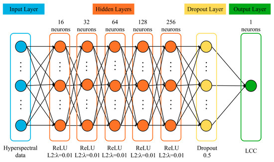
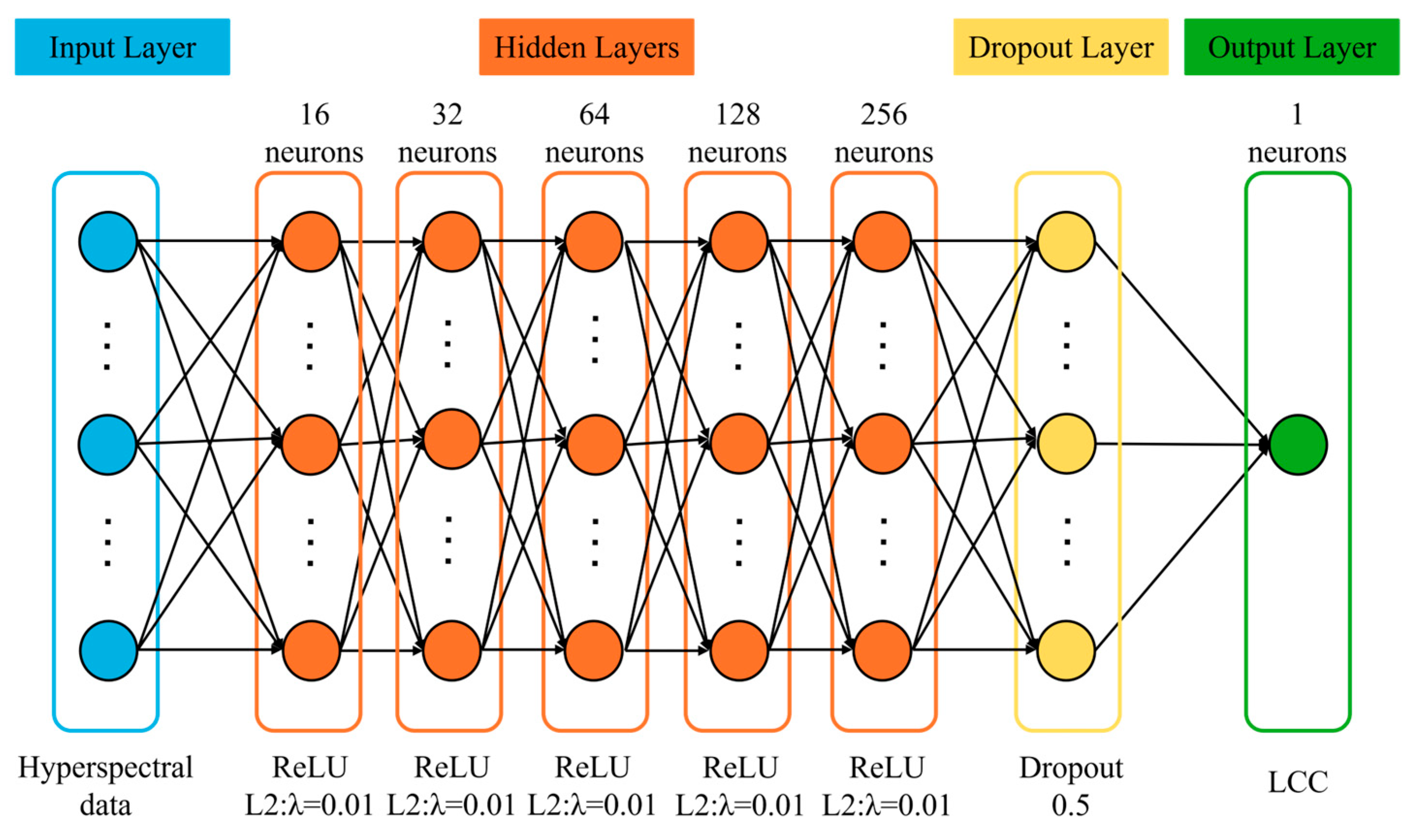
To combine the mechanistic advantages of physical models with the data adaptability of domain learning, a hybrid model, PROSAIL-DNN-TL, based on PROSAIL and TL was constructed. This hybrid approach comprises two stages: pre-training and fine-tuning. First, the DNN model was pre-trained using the PROSAIL simulation dataset. Subsequently, the pre-trained model was fine-tuned using measured hyperspectral data through a full-network fine-tuning strategy. During this process, all network parameters inherited from the PROSAIL pre-training stage were updated to adapt the model to the spectral characteristics of actual winter wheat canopies. The PROSAIL-DNN-TL model adopts a neural network architecture comprising five fully connected hidden layers (Figure 4), with the ReLU activation function and a linear regression layer as the output layer. To suppress model overfitting, L2 regularisation (λ = 0.01) was applied to each hidden layer, and a dropout layer (0.5) was added after the final hidden layer to enhance generalisation ability. During the pre-training phase, the Adam optimiser was used with an initial learning rate of 0.005 and an exponential decay strategy (decay factor 0.98), with a maximum of 500 training iterations and an early stopping mechanism patience of 30. During the fine-tuning phase, building upon the pre-trained weights, the Adam optimiser was used with a lower initial learning rate (0.001). The learning rate was halved every 50 iterations, with a maximum of 300 training iterations and an early stopping threshold adjusted to 20. The same measured training dataset was used for training the machine learning models and fine-tuning the DNN-based models, ensuring a fair comparison among different modelling approaches.
Figure 4.
DNN Framework Diagram.
To evaluate the effectiveness of incorporating PROSAIL-based pre-training, a DNN model trained directly on real hyperspectral data was set as the control. The DNN employs exactly the same network architecture, regularisation and dropout settings as the PROSAIL-DNN-TL; the only differences lie in the initialisation method and training parameters: the model weights are randomly initialised, the Adam optimiser is used during the training phase with an initial learning rate of 0.005 and no active decay strategy, the maximum number of training iterations is 500, and the patience value for the early stopping mechanism is set to 30.
In this study, 500 independent deep learning experiments were conducted. Different random seeds were used for stratified data partitioning in each experiment, and the corresponding model performance metrics were recorded. The mean and standard deviation of the evaluation metrics across the 500 repetitions were calculated to assess model stability and performance variability (Table S1). For visualization purposes, a representative model was selected from the 500 repetitions based on its validation loss and overall performance consistency with the mean results. The selected model weights were subsequently used for LCC prediction using datasets collected during the two growing seasons.
2.4.3. Model Evaluation
Model performance was evaluated using the coefficient of determination R2, root mean square error (RMSE), relative root mean square error (RRMSE) and mean absolute error (MAE). The closer R2 is to 1, the higher the predictive accuracy of the model; the smaller the values of RMSE, RRMSE and MAE, the better the model performance. The calculation formulas are as follows:
where y and yi represent the observed chlorophyll content and the model-derived predicted value for each sample, respectively; and and represent the observed mean and the mean of the derived values for the samples, respectively; n is the number of samples.
3. Results
3.1. Feature Selection
Feature selection is an essential step in statistical analysis and data modelling, aiming to identify the most informative variables associated with the target parameter while reducing redundant information [47].
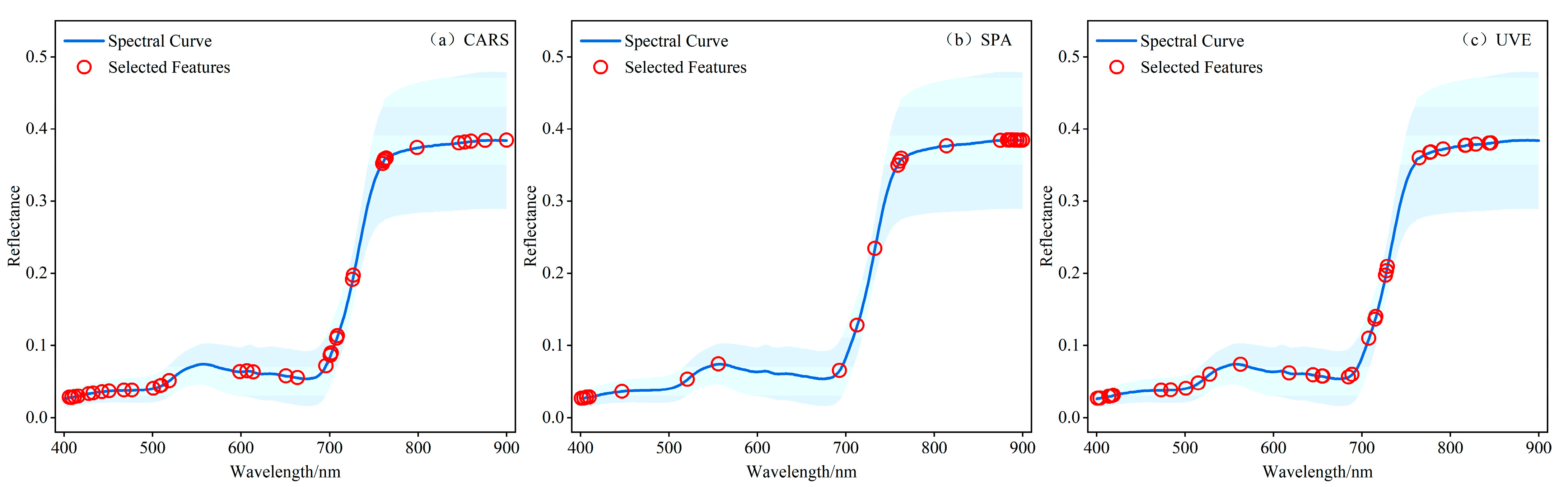
As shown in Figure 5, the CARS algorithm retained 36 spectral bands, which were distributed across the visible, red-edge and near-infrared regions. Compared with the other two feature selection methods, CARS selected more bands in the visible region. The SPA retained 22 bands, with most selected wavelengths concentrated in the near-infrared region, while fewer bands were selected from the visible and red-edge regions. The UVE algorithm selected 33 bands, and the selected wavelengths showed a relatively more balanced distribution across different spectral regions compared with CARS and SPA.
Figure 5.
Results of different feature selection methods. (a) CARS, (b) SPA, and (c) UVE. Among them, the light blue background represents the standard deviation of the average wheat spectrum curve.
3.2. Analysis of Machine Learning Models Based on Different Feature Sets
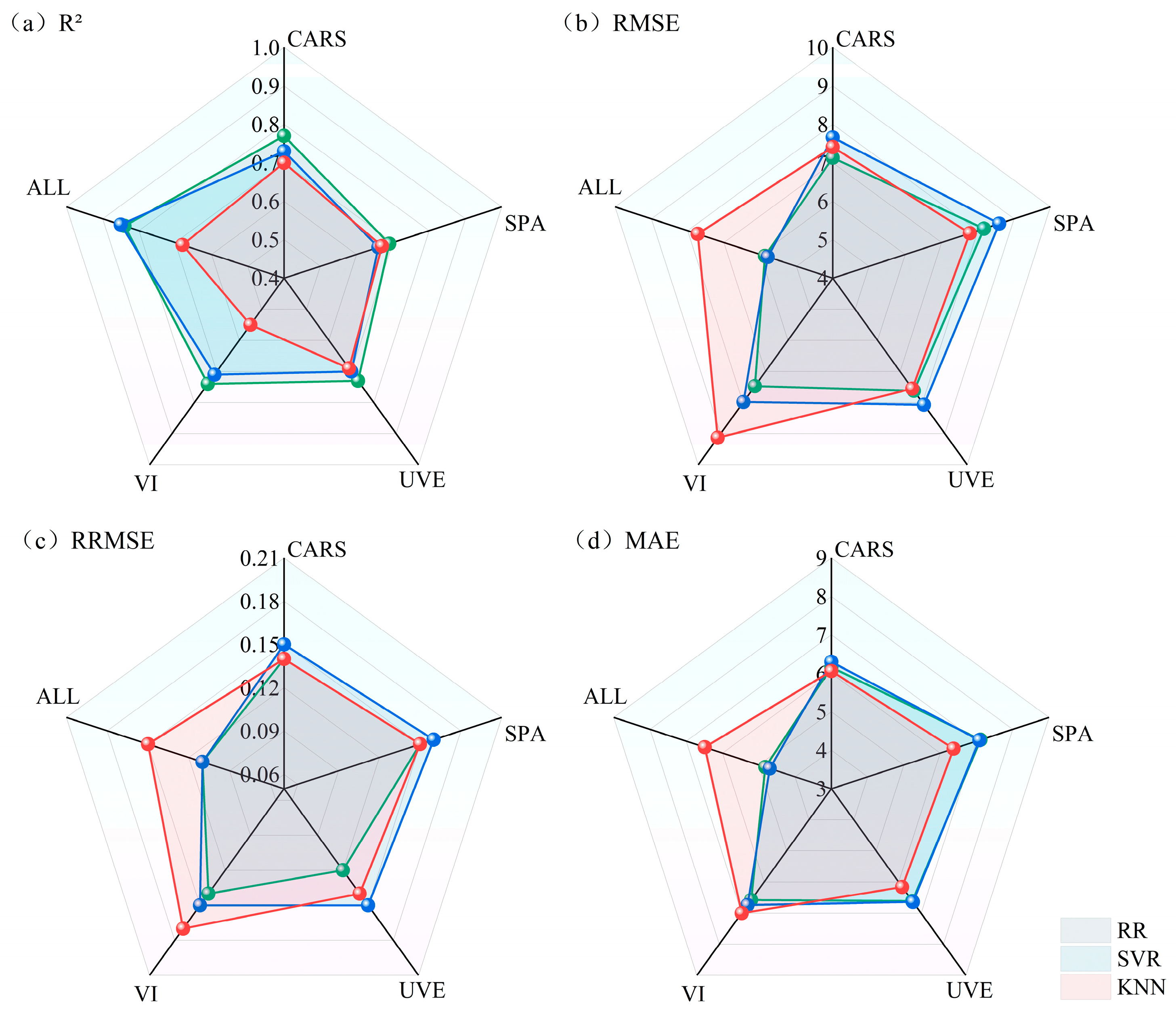
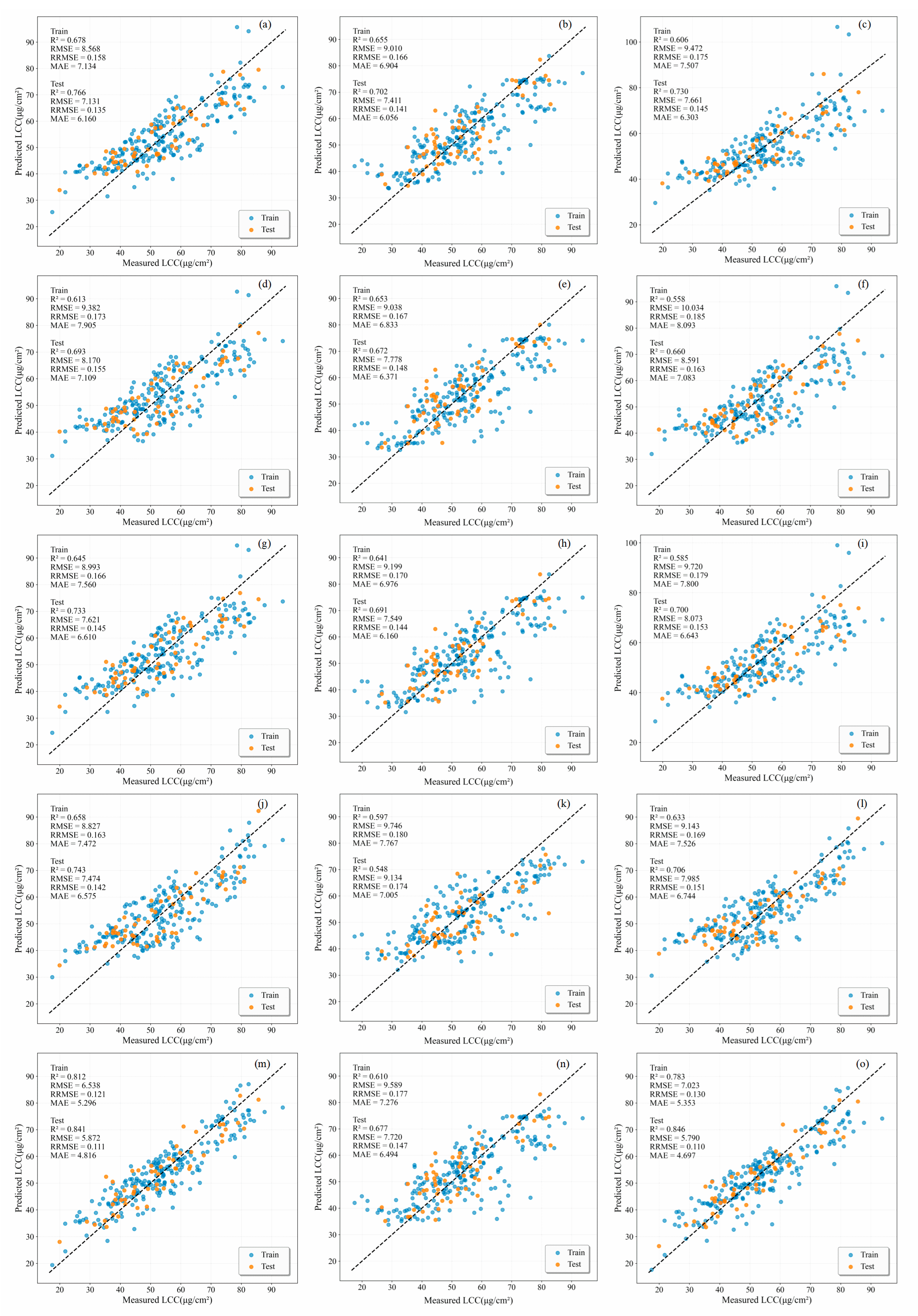
The accuracy of the monitoring models based on different feature sets and machine learning methods is shown in Figure 6 and Figure 7. Overall, the RR model performed best, achieving the highest monitoring accuracy, whilst the KNN model performed relatively poorly. The performance of the datasets varied depending on the machine learning method used: the RR and SVR models exhibited the same trend, with the ALL feature set achieving the highest accuracy, followed by the CARS and VI feature sets, and finally the UVE and SPA feature sets; the KNN model, however, yielded different results, with the CARS feature set achieving the highest accuracy, followed by the ALL and UVE feature sets, and finally the SPA and VI feature sets. Compared with the SPA and UVE methods, CARS performed best, with the RR model achieving the highest R2 value (0.77).
Figure 6.
Comparison of machine learning model results based on different feature selection methods.
Figure 7.
Measured and predicted LCC based on different machine learning methods and feature sets. (a) CARS-RR, (b) CARS-KNN, (c) CARS-SVR, (d) SPA-RR, (e) SPA-KNN, (f) SPA-SVR, (g) UVE-RR, (h) UVE-KNN, (i) UVE-SVR, (j) VI-RR, (k) VI-KNN, (l) VI-SVR, (m) ALL-RR, (n) ALL-KNN, (o) ALL-SVR.
3.3. Comparison and Analysis of Deep Learning Models
The evaluation results of machine learning models based on different feature sets demonstrated that the ALL feature set achieved the best overall performance; therefore, this feature set was selected for subsequent deep learning model development. The performance comparison of different modelling approaches using the same feature set is presented in Table 4. Based on 500 repeated stratified random experiments, all deep learning models achieved reliable estimation performance for winter wheat LCC, with test-set R2 values close to 0.79 and RMSE values approximately 6.75 μg/cm2.
Table 4.
Comparison of Accuracy of Different Models Based on the Same Dataset.
Compared with the conventional DNN model, the PROSAIL-DNN-TL model showed significantly improved performance on the training dataset. The training-set R2 increased from 0.841 ± 0.042 to 0.894 ± 0.035, while the RMSE, RRMSE, and MAE decreased from 5.948 ± 0.764 to 4.849 ± 0.739 μg/cm2, from 0.110 ± 0.014 to 0.090 ± 0.014, and from 4.643 ± 0.628 to 3.625 ± 0.619 μg/cm2, respectively (p < 0.001). For the test dataset, no significant differences were observed between PROSAIL-DNN-TL and DNN in R2, RMSE, and RRMSE (p > 0.05). However, the MAE of PROSAIL-DNN-TL was significantly lower than that of DNN (5.159 ± 0.674 vs. 5.300 ± 0.632 μg/cm2, p < 0.001).
Furthermore, both the PROSAIL-DNN-TL and DNN models showed better average prediction performance than the evaluated machine learning models (SVR, KNN, and RR), with lower RMSE, MAE and RRMSE values. These results indicate the potential of deep learning models for LCC monitoring under the experimental conditions of this study.
Paired statistical analyses were conducted based on the 500 repeated experiments using identical random seeds. The differences between the two models were calculated for each evaluation metric, followed by normality testing and paired statistical tests (Table 5). The results showed that PROSAIL-DNN-TL significantly improved the training performance compared with DNN, with significant differences observed in R2, RMSE, RRMSE and MAE (p < 0.001). However, no significant differences were observed for most testing metrics, including R2, RMSE and RRMSE (p > 0.05), while MAE showed a significant difference between the two models (p < 0.001). These results indicate that PROSAIL-DNN-TL achieved comparable predictive performance to DNN on the test samples, while providing improved fitting capability during training.
Table 5.
Statistical significance analysis of performance differences between PROSAIL-DNN-TL and DNN models based on 500 repeated experiments.
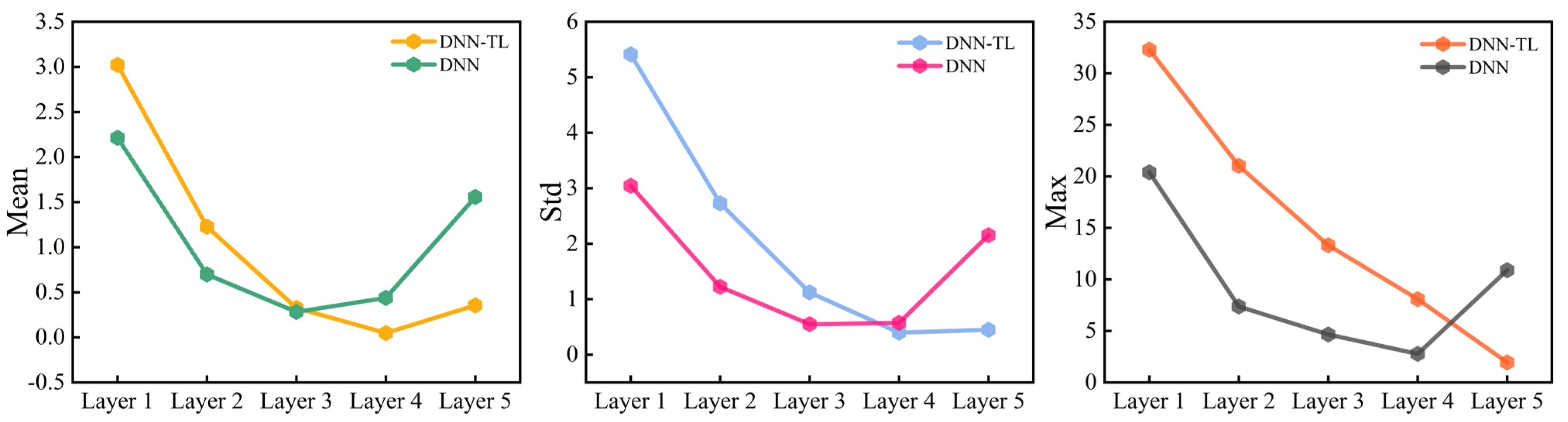
To further investigate the feature representation differences between PROSAIL-DNN-TL and DNN, the hidden features extracted from each layer of the two models were statistically analysed, and the results are presented in Figure 8. In the shallow layers (layers 1–3), the mean, standard deviation and maximum values of the hidden features extracted by PROSAIL-DNN-TL were generally higher than those of the DNN model.
Figure 8.
Comparison of hidden layer data between the optimal models of PROSAIL-DNN-TL and DNN. The line plots show the mean, standard deviation, and maximum values of the extracted features from the five hidden layers of each model. The comparison illustrates differences in feature distributions between the transfer learning-based model and the directly trained DNN model. In the figure, “DNN-TL” refers to the PROSAIL-DNN-TL model.
3.4. Evaluation of LCC Monitoring Performance Using Data Collected During Two Growing Seasons
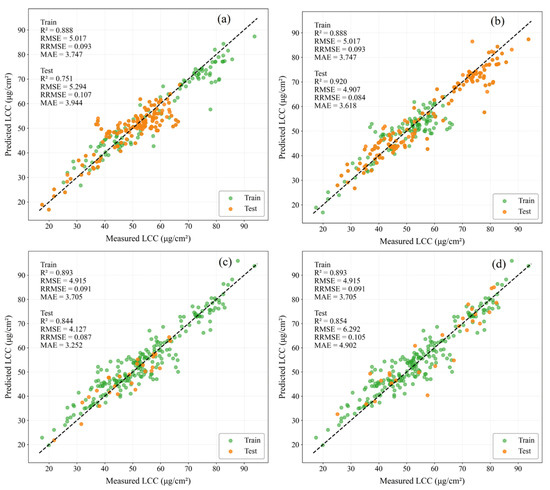
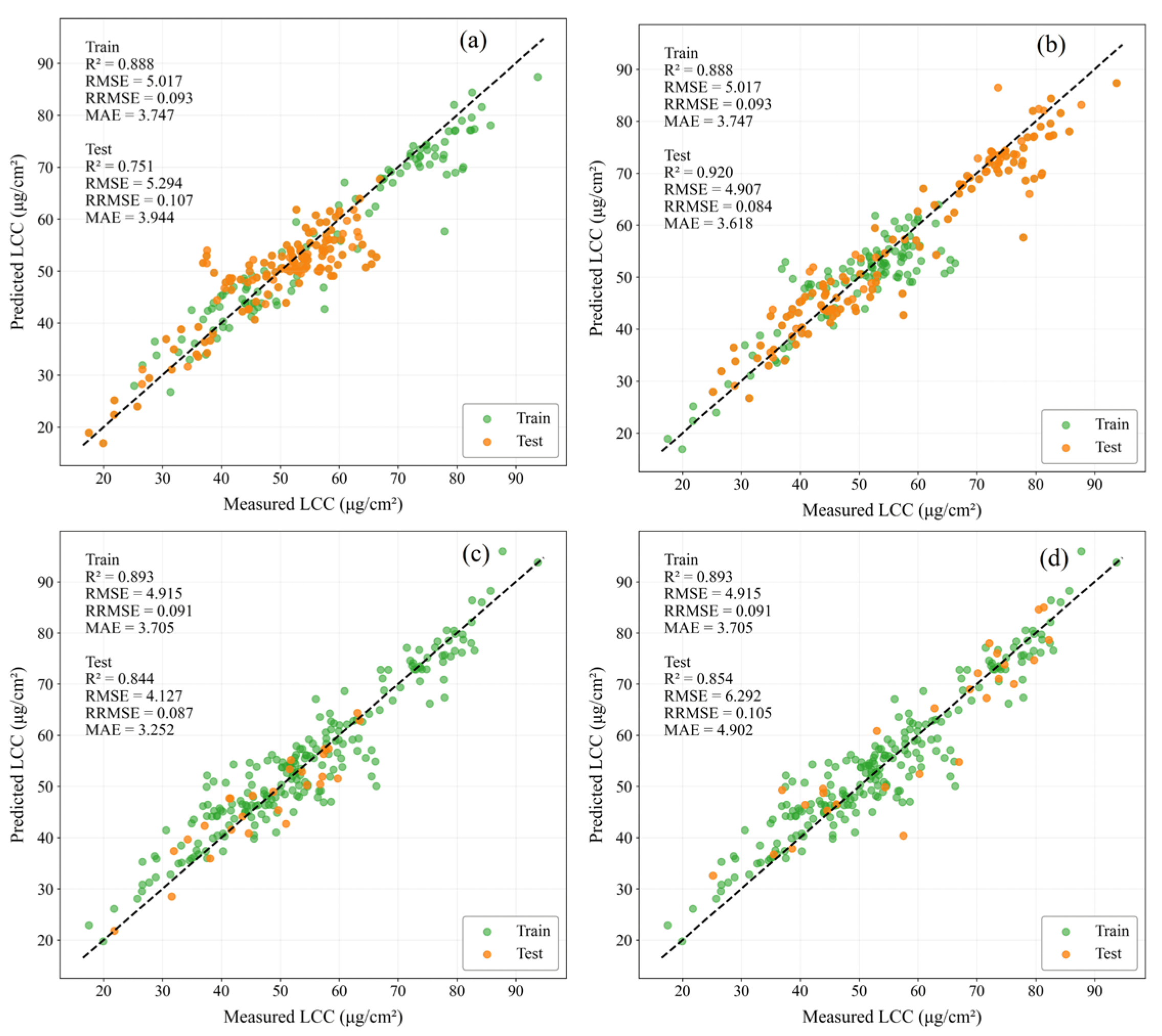
The evaluation results showed that the PROSAIL-DNN-TL model achieved competitive predictive performance among the evaluated models. Therefore, the optimal PROSAIL-DNN-TL model obtained from the 500 stratified random experiments was selected to further evaluate its predictive performance on datasets collected during the two growing seasons. As shown in Figure 9, the PROSAIL-DNN-TL model achieved an R2 of 0.75, an RMSE of 5.29 μg/cm2, an RRMSE of 0.12%, and an MAE of 3.94 μg/cm2 for the 2024 dataset; for the 2025 dataset, the model achieved an R2 of 0.92, an RMSE of 4.91 μg/cm2, an RRMSE of 0.08%, and an MAE of 3.62 μg/cm2. These results indicate that the PROSAIL-DNN-TL model pre-trained using PROSAIL simulated data achieved reliable predictive performance on the testing datasets collected during the two growing seasons included in this study.
Figure 9.
Accuracy assessment of the optimal models on testing datasets collected during two growing seasons: (a) PROSAIL-DNN-TL model evaluated using the 2024 growing season testing dataset; (b) PROSAIL-DNN-TL model evaluated using the 2025 growing season testing dataset; (c) DNN model evaluated using the 2024 growing season testing dataset; (d) DNN model evaluated using the 2025 growing season testing dataset.
To further compare the predictive performance of PROSAIL-DNN-TL and DNN models, the DNN model was assessed using the same evaluation strategy (Figure 9). The DNN model achieved an R2 of 0.84, an RMSE of 4.13 μg/cm2, an RRMSE of 0.09%, and an MAE of 3.25 μg/cm2 for the 2024 dataset; for the 2025 dataset, the corresponding values were 0.85, 6.29 μg/cm2, 0.11%, and 4.90 μg/cm2, respectively.
Furthermore, for comparison with the PROSAIL-DNN-TL model, the optimal machine learning model was evaluated using the testing datasets from the two growing seasons. Among 100 rounds of random stratified cross-validation, the SVR model (linear kernel, C = 2, epsilon = 0.1) achieved the best performance. However, when this optimal model was evaluated on testing datasets collected during the two growing seasons, the test-set R2 values were −0.57 and −1.91, respectively, indicating that the performance of traditional machine learning models varied when directly applied to datasets collected from different growing seasons without additional model adjustment.
4. Discussion
4.1. Analysis of Machine Learning Models Using Different Feature Sets
The better average performance of the CARS-based models may be attributed to the effective identification of informative spectral regions associated with LCC variation. Previous studies have demonstrated that chlorophyll-related parameters are highly sensitive to spectral responses in the visible and red-edge regions [48], where strong absorption by chlorophyll pigments and changes in leaf structure contribute to variations in reflectance characteristics [49]. Therefore, retaining informative wavelengths from these regions may provide more effective spectral signals for LCC estimation [50]. The superior performance of CARS can be attributed to its feature selection mechanism. CARS combines Monte Carlo sampling with partial least squares regression coefficients, adaptively assigning weights to spectral bands during the iterative selection. It preferentially retains wavelengths strongly associated with LCC and removes redundant or noisy information, thereby improving model efficiency and predictive performance. Although feature selection methods can reduce data dimensionality and computational complexity, the selected feature subsets obtained by SPA and UVE did not consistently outperform the full-spectrum dataset, which is consistent with previous findings reported by Chen et al. [37].
The VI developed in this study did not significantly improve LCC estimation accuracy and showed relatively lower performance among all feature datasets. This may be attributed to the fact that VIs are generally constructed using fixed combinations of several spectral bands, such as ratios, differences or normalised formulations [51]. Although VIs can effectively characterize crop growth status, their robustness may decrease when spectral signals are affected by external factors, including soil background, canopy structure, and leaf water content. In addition, environmental fluctuations during field measurement may influence the stability of sensitive spectral regions and subsequently affect VI-based estimation [52].
During the extraction of characteristic wavelengths, the selected wavelengths may result in the loss of some information, failing to fully represent all the information in the original dataset, thereby affecting subsequent data analysis and modelling [53]. In this study, RR and SVR achieved higher accuracy using the ALL dataset, which may be attributed to their ability to exploit the complete spectral information contained in hyperspectral variables. Hyperspectral data usually exhibit strong correlations among adjacent bands, resulting in multicollinearity and redundant information [54]. RR can alleviate the adverse effects of multicollinearity by introducing L2 regularization, thereby improving model stability when using high-dimensional spectral variables [43]. Meanwhile, SVR can effectively capture nonlinear relationships between spectral reflectance and LCC through kernel functions, making it suitable for modelling complex spectral–biophysical relationships [55]. In contrast, KNN relies on the similarity between samples calculated from feature distances and is therefore more sensitive to the dimensionality of the feature space. The inclusion of redundant spectral bands may reduce the reliability of neighbour selection in high-dimensional spaces, leading to decreased prediction performance. This phenomenon is consistent with the well-known curse of dimensionality problem associated with distance-based algorithms [56], which may explain why KNN achieved better performance using feature-selected datasets rather than the full-spectrum dataset.
4.2. Performance Analysis of LCC Monitoring Using Deep Transfer Learning
The results of this study indicate that, under the conditions of this case study, the transfer learning-based model achieved comparable predictive performance to the directly trained DNN model, while showing improved performance compared with the evaluated machine learning models. This finding is consistent with previous studies reporting the effectiveness of transfer learning approaches for crop trait estimation [57,58].
The evaluations based on data collected from the two growing seasons showed different relative performances between the PROSAIL-DNN-TL and DNN models under the experimental conditions of this study. PROSAIL-DNN-TL showed higher accuracy on the 2025 dataset, whereas DNN showed better performance on the 2024 dataset. Analysis of the measured LCC distributions (Table 1, Figure 3) suggested that differences in environmental conditions and trait distributions between years may have contributed to this discrepancy. In 2025, drought stress accelerated crop development and resulted in a wider LCC distribution, covering a more complete gradient from low to high values. This broader distribution may have facilitated the PROSAIL-DNN-TL model in exploiting the physical prior information obtained from PROSAIL simulations. In contrast, the LCC distribution in 2024 was relatively concentrated, increasing the discrepancy between simulated and measured characteristics and limiting the adaptation ability of the transfer learning model. Consequently, the fine-tuning effect of PROSAIL-DNN-TL was relatively limited in 2024.
In comparison, the DNN model was entirely data-driven and was not constrained by the range of physical priors provided by PROSAIL. Therefore, it maintained relatively stable predictive performance across both years, demonstrating stable predictive performance under the evaluated datasets. Therefore, it maintained relatively stable predictive performance across both years, demonstrating strong adaptability to variations in measured datasets.
Most crop monitoring studies rely on empirical machine learning models, whose performance is highly dependent on sample size, feature selection and modelling strategies [59,60,61]. In this study, the relationship between LCC and spectral characteristics represents a complex nonlinear relationship affected by multiple factors, including canopy structure, soil background and environmental conditions. Traditional machine learning models generally have shallow structures and therefore have limited ability to extract deep features and complex relationships from high-dimensional hyperspectral data, particularly when the number of samples is limited [62]. In contrast, deep learning models can automatically learn complex nonlinear relationships between spectral information and crop traits through hierarchical network structures, thereby improving predictive capability [63]. Both PROSAIL-DNN-TL and DNN models employ deep architectures consisting of multiple fully connected layers, allowing progressive extraction of high-level spectral features and improving LCC inversion performance [64].
However, deep learning methods generally require large amounts of labelled data and involve high computational costs [65,66]. Transfer learning provides an effective strategy to reduce dependence on extensive labelled datasets by transferring knowledge learned from related domains [67]. In this study, RTM was integrated with transfer learning. PROSAIL simulations were used to learn the physical relationship between spectral responses and LCC under different conditions [68], providing prior knowledge for subsequent estimation using field-measured data [48]. Due to the physical consistency between simulated and real canopy spectral responses, the pre-trained model can provide effective initial feature representations for LCC estimation [69]. After transferring to measured datasets, only fine-tuning was required to optimize the model parameters according to the measured LCC distribution of winter wheat, thereby improving prediction performance. The paired statistical tests (Table 5) showed that pre-training with PROSAIL simulations enhanced the model’s ability to learn physically meaningful spectral, canopy, and LCC relationships and resulted in different hidden feature distributions during model optimization. However, although the incorporation of physical prior knowledge improved the learning process, the limited number of field samples may constrain further improvements in independent prediction performance. Nevertheless, PROSAIL-DNN-TL achieved a significant reduction in testing MAE, indicating that the proposed transfer learning framework can reduce prediction deviations and improve model reliability under limited sample conditions. Similarly, Figure 8 illustrates the differences in hidden feature distributions between the PROSAIL-DNN-TL and DNN models across different network layers. This indicates that the pre-training process resulted in different initial feature representations, which contributed to the preservation and transmission of spectral and canopy structural information. In contrast, for the deeper layers (layers 4–5), the statistical values of PROSAIL-DNN-TL were lower than those of DNN, suggesting that fine-tuning allowed the model to better adapt its feature representations to the actual LCC distribution of winter wheat.
4.3. Future Prospects and Limitations
Although the proposed PROSAIL-DNN-TL framework achieved satisfactory performance for winter wheat LCC estimation, several limitations should be acknowledged.
First, uncertainty may exist in the conversion of SPAD values into LCC because the empirical equation used in this study was originally developed based on Minolta SPAD-502 measurements of broadleaf species. Differences in crop type, leaf anatomical characteristics, and sensor optical properties between the original calibration dataset and the present study may affect the accuracy of absolute LCC estimation. Future studies should establish crop- and instrument-specific SPAD-LCC calibration models using simultaneous SPAD measurements and destructive chlorophyll determination. In addition, although sampling dates were determined according to observed phenological stages, emergence dates and cumulative growing degree days (GDD) were not recorded during the field experiment. Future studies should incorporate DAE and GDD information together with phenological observations to provide a more quantitative description of crop development dynamics across different growing seasons.
Second, although the PROSAIL model used in this study was parameterised according to winter wheat characteristics, the physical basis of PROSAIL allows its application to different crops by adjusting leaf structural parameters, biochemical composition and canopy geometric parameters. Therefore, the proposed framework has the potential to be extended to other crops, such as soya beans, rice, cotton and maize. However, this transferability has not yet been experimentally validated. Future studies should evaluate the applicability of the PROSAIL-DNN-TL model across different crop types and environments. In addition, PROSAIL simulations can generate more diverse data by incorporating variations in soil reflectance, atmospheric conditions and observation geometries. Cross-regional validation in different soil backgrounds (e.g., black soil, red soil and yellow loamy soil regions) and climatic zones with different accumulated temperatures is required to further assess the performance of the model under different environmental conditions. Future studies could integrate three-dimensional RTMs (e.g., LESS and DART) and crop growth simulation models (e.g., DSSAT and WOFOST) to construct more realistic simulated datasets that better represent field conditions.
Third, although the proposed simulation and fine-tuning strategies are not restricted to a specific DNN architecture, the current study only evaluated a fully connected neural network. Future research could extend this framework to other regression architectures, such as LSTM and Transformer models, to investigate their ability to capture temporal dynamics in spectral sequences and long-range dependencies among spectral bands, and to determine their effects on LCC inversion accuracy under different experimental scenarios.
In this study, the measured samples were divided into independent training and testing subsets, and only the training samples were used for model fine-tuning. Therefore, no information from the test dataset was involved in model optimisation. However, the fine-tuning dataset only covered two growing seasons, and the model was not evaluated using data from completely unseen growing seasons or regions. Therefore, the applicability of the proposed framework under broader environmental conditions remains to be further investigated. Future studies should incorporate additional growing seasons and more diverse field conditions into the fine-tuning process to provide richer real-world spectral patterns and improve model reliability. In addition, the influence of the amount of measured data required for fine-tuning remains unclear. Future studies could investigate the sensitivity of model performance to different proportions of available field samples (e.g., 20%, 40%, 60% and 80%) to evaluate model robustness under limited data conditions and inform practical field sampling strategies.
Finally, although hidden-layer analysis was conducted to explore the feature representation capability of the proposed model, the interpretability of deep learning models remains limited. Future studies should combine advanced visualisation and feature attribution methods to provide deeper insights into the hierarchical abstraction of spectral features and their relationships with LCC. Moreover, validation using publicly available datasets collected from different regions will be essential to further improve the reliability and practical applicability of the proposed framework.
5. Conclusions
This study proposed a hybrid model, PROSAIL-DNN-TL, which integrates the PROSAIL RTM with transfer learning for winter wheat LCC estimation. By comparing it with traditional machine learning models using different feature sets and a DNN model trained with measured data, this study evaluated the potential of combining physical simulations and deep learning for hyperspectral-based crop monitoring. The main conclusions are as follows:
- (1)
- Comparison of the three feature selection methods (CARS, SPA and UVE) showed that the UVE-selected bands were relatively evenly distributed across the visible, red-edge and near-infrared regions. In contrast, the CARS-selected bands were mainly distributed in the visible region, whereas the SPA-selected bands were primarily concentrated in the near-infrared region.
- (2)
- Machine learning models based on different feature sets demonstrated that RR and SVR generally achieved higher accuracy than KNN. The ALL and CARS feature sets showed relatively better performance, followed by the UVE and VI, whilst SPA exhibited the lowest accuracy, indicating that the selection and completeness of spectral information strongly affected model performance.
- (3)
- Based on the mean performance across repeated experiments, the PROSAIL-DNN-TL model showed competitive performance for winter wheat LCC estimation among all evaluated approaches. The model obtained an average testing R2 of 0.79, which was comparable to that of the DNN model (R2 = 0.79). Statistical analysis showed that PROSAIL-DNN-TL significantly improved training performance and reduced testing MAE, while no significant differences were observed in other testing metrics compared with DNN. Compared with the optimal machine learning model, the PROSAIL-DNN-TL showed a higher average testing R2 by approximately 0.05.
This study indicates that combining PROSAIL-based pre-training with measured-data fine-tuning provides a potential strategy for incorporating simulated spectral information into deep learning models for winter wheat LCC estimation. However, the SPAD-to-LCC conversion used in this study was not specifically calibrated for the instrument and crop, and therefore, the absolute LCC values should be interpreted with caution. Future studies should establish crop- and instrument-specific SPAD-LCC calibration models using simultaneous SPAD measurements and destructive chlorophyll determination to improve the accuracy and interpretability of absolute LCC estimates.
Supplementary Materials
The following are available online at https://www.mdpi.com/article/10.3390/agronomy16191971/s1, Table S1: Means and standard deviations of the performance metrics for different models on the training and test sets.
Author Contributions
Conceptualization, X.Z. and X.L.; methodology, X.Z.; software, X.Z.; validation, X.Z., Y.N. and J.L.; formal analysis, X.Z.; investigation, X.Z.; resources, X.Z.; data curation, X.Z.; writing—original draft preparation, X.Z.; writing—review and editing, X.Z.; visualization, X.Z.; supervision, Y.N., J.L. and X.L.; project administration, Y.N., J.L. and X.L.; funding acquisition, Y.N., J.L. and X.L. All authors have read and agreed to the published version of the manuscript.
Funding
This research was funded by Industry–University–Research Collaboration Projects (Nos. 20240028, 20250019, 20250304, and 20250315), the Natural Science Research Project of Universities in Anhui Province (No. 2023AH051856), and the Anhui Province Agricultural Science and Technology Modernization Pilot County Project (No. 882443).
Data Availability Statement
The datasets presented in this article are not readily available because the data are part of an ongoing study. Requests to access the datasets should be directed to the corresponding author.
Acknowledgments
Artificial intelligence (Doubao(web version, accessed in May 2026; version number not specified)) was used during the preparation of this manuscript to assist in improving language, restructuring sentences, and enhancing the clarity of scientific writing in selected parts of the text. No generative AI tools were used for data extraction, statistical modeling, analysis or interpretation of results, and especially not for scientific decision-making. All content was meticulously reviewed by the authors, who assume full responsibility for the final version of the manuscript.
Conflicts of Interest
The authors declare no conflicts of interest.
Abbreviations
The following abbreviations are used in this manuscript:
| CARS | Competitive adaptive reweighted sampling |
| DL | Deep learning |
| DNN | Deep neural network |
| KNN | K-Nearest Neighbors |
| LCC | Leaf chlorophyll content |
| MAE | Mean absolute error |
| ML | Machine learning |
| R2 | Coefficient of determination |
| RMSE | Root mean square error |
| RR | Ridge Regression |
| RRMSE | Relative root mean square error |
| RTMs | Radiative transfer models |
| SPA | Successive projections algorithm |
| SVR | Support Vector Regression |
| TL | Transfer learning |
| UVE | Uninformative variable elimination |
| VI | Vegetation index |
References
- Croft, H.; Chen, J.M.; Luo, X.; Bartlett, P.; Chen, B.; Staebler, R.M. Leaf chlorophyll content as a proxy for leaf photosynthetic capacity. Glob. Change Biol. 2017, 23, 3513–3524. [Google Scholar] [CrossRef] [Scilit] [PubMed]
- Sonobe, R.; Hirono, Y. Carotenoid content estimation in tea leaves using noisy reflectance data. Remote Sens. 2023, 15, 4303. [Google Scholar] [CrossRef] [Scilit]
- Shen, Y.Y.; Meng, R.; Li, J.S.; Zhao, P.; Zhao, F.; Sun, R.; Zhang, H.Y.; Ni, X.; Lu, L.J.; Liu, Y.; et al. A hybrid method for major food crops leaf chlorophyll content inversion driven by remote sensing mechanisms and deep learning. Nat. Remote Sens. Bull. 2026, 30, 1392–1412, (In Chinese with English abstract). [Google Scholar]
- Zhu, X.; Li, J.; Sheng, Y.; Wang, W.; Wang, H.; Yang, H.; Nian, Y.; Liu, J.; Li, X. How Do Spectral Scales and Machine Learning Affect SPAD Monitoring at Different Growth Stages of Winter Wheat? Agriculture 2025, 15, 2410. [Google Scholar] [CrossRef] [Scilit]
- Osco, L.P.; Ramos, A.P.M.; Moriya, É.A.S.; Bavaresco, L.G.; Lima, B.C.; Estrabis, N.; Pereira, D.R.; Creste, J.E.; Júnior, J.M.; Gonçalves, W.N.; et al. Modeling Hyperspectral Response of Water-Stress Induced Lettuce Plants Using Artificial Neural Networks. Remote Sens. 2019, 11, 2797. [Google Scholar] [CrossRef] [Scilit]
- Curran, P.J. Remote sensing of foliar chemistry. Remote Sens. Environ. 1989, 30, 271–278. [Google Scholar] [CrossRef] [Scilit]
- Li, D.; Chen, J.M.; Yu, W.; Zheng, H.; Yao, X.; Cao, W.; Wei, D.; Xiao, C.; Zhu, Y.; Cheng, T. Assessing a soil-removed semi-empirical model for estimating leaf chlorophyll content. Remote Sens. Environ. 2022, 282, 113284. [Google Scholar] [CrossRef] [Scilit]
- Wan, L.; Liu, Y.; He, Y.; Cen, H. Prior knowledge and active learning enable hybrid method for estimating leaf chlorophyll content from multi-scale canopy reflectance. Comput. Electron. Agric. 2023, 214, 108308. [Google Scholar] [CrossRef] [Scilit]
- Chakhvashvili, E.; Siegmann, B.; Muller, O.; Verrelst, J.; Bendig, J.; Kraska, T.; Rascher, U. Retrieval of Crop Variables from Proximal Multispectral UAV Image Data Using PROSAIL in Maize Canopy. Remote Sens. 2022, 14, 1247. [Google Scholar] [CrossRef] [Scilit] [PubMed]
- Berger, K.; Atzberger, C.; Danner, M.; D’Urso, G.; Mauser, W.; Vuolo, F.; Hank, T. Evaluation of the PROSAIL Model Capabilities for Future Hyperspectral Model Environments: A Review Study. Remote Sens. 2018, 10, 85. [Google Scholar] [CrossRef] [Scilit]
- Zhao, D.; Yang, G.; Xu, T.; Yu, F.; Zhang, C.; Cheng, Z.; Ren, L.; Yang, H. Dynamic maize true leaf area index retrieval with KGCNN and TL and integrated 3D radiative transfer modeling for crop phenotyping. Plant Phenomics 2025, 7, 100004. [Google Scholar] [CrossRef] [Scilit] [PubMed]
- Haq, A.U.; Li, J.P.; Khan, I.; Agbley, B.L.Y.; Ahmad, S.; Uddin, M.I.; Zhou, W.; Khan, S.; Alam, I. DEBCM: Deep Learning-Based Enhanced Breast Invasive Ductal Carcinoma Classification Model in IoMT Healthcare Systems. IEEE J. Biomed. Health Inform. 2024, 28, 1207–1217. [Google Scholar] [CrossRef] [Scilit] [PubMed]
- Shimodaira, H. Improving predictive inference under covariate shift by weighting the log-likelihood function. J. Stat. Plan. Inference 2000, 90, 227–244. [Google Scholar] [CrossRef] [Scilit]
- LeCun, Y.; Bengio, Y.; Hinton, G. Deep learning. Nature 2015, 521, 436–444. [Google Scholar] [CrossRef] [Scilit] [PubMed]
- Bengio, Y.; Courville, A.; Vincent, P. Representation learning: A review and new perspectives. arXiv 2014, arXiv:1206.5538. [Google Scholar]
- Alpaydin, E. Introduction to Machine Learning; MIT Press: Cambridge, MA, USA, 2014. [Google Scholar]
- Voulodimos, A.; Doulamis, N.; Doulamis, A.; Protopapadakis, E. Deep Learning for Computer Vision: A Brief Review. Comput. Intell. Neurosci. 2018, 2018, 7068349. [Google Scholar] [CrossRef] [Scilit] [PubMed]
- Kumar, J.S.; Anuar, S.; Hassan, N.H. Transfer Learning Based Performance Comparison of the Pre-Trained Deep Neural Networks. Int. J. Adv. Comput. Sci. Appl. 2022, 13, 1. [Google Scholar] [CrossRef] [Scilit]
- Lu, C.; Li, W. Ship Classification in High-Resolution SAR Images via Transfer Learning with Small Training Dataset. Sensors 2019, 19, 63. [Google Scholar] [CrossRef] [Scilit] [PubMed]
- Signorelli, C.M. Can Computers Become Conscious and Overcome Humans? Front. Robot. AI 2018, 5, 121. [Google Scholar] [CrossRef] [Scilit] [PubMed]
- Chollet, F. Deep Learning with Python; Manning Publications: Shelter Island, NY, USA, 2017. [Google Scholar]
- Marcus, G.F. Rethinking Eliminative Connectionism. Cogn. Psychol. 1998, 37, 243–282. [Google Scholar] [CrossRef] [Scilit] [PubMed]
- Ribeiro, M.T.; Singh, S.; Guestrin, C. “Why Should I Trust You?”: Explaining the Predictions of Any Classifier. arXiv 2016, arXiv:1602.04938. [Google Scholar]
- Tsimenidids, S. Limitations of Deep Neural Networks: A Discussion of G. Marcus’ Critical Appraisal of Deep Learning. arXiv 2020, arXiv:2012.15754. [Google Scholar]
- Shrestha, A.; Mahmood, A. Review of deep learning algorithms and architectures. IEEE Access 2019, 7, 53040–53065. [Google Scholar] [CrossRef] [Scilit]
- Palanichamy, K. Integrative omic analysis of neuroblastoma. In Computational Epigenetics and Diseases; Academic Press: London, UK, 2019; pp. 311–326. [Google Scholar]
- Tsiakmaki, M.; Kostopoulos, G.; Kotsiantis, S.; Ragos, O. Transfer Learning from Deep Neural Networks for Predicting Student Performance. Appl. Sci. 2020, 10, 2145. [Google Scholar] [CrossRef] [Scilit]
- Pan, S.J.; Yang, Q. A survey on transfer learning. IEEE Trans. Knowl. Data Eng. 2010, 22, 1345–1359. [Google Scholar] [CrossRef] [Scilit]
- Weiss, K.; Khoshgoftaar, T.M.; Wang, D. A survey of transfer learning. J. Big Data 2016, 3, 9. [Google Scholar] [CrossRef] [Scilit]
- Zhuang, F.; Qi, Z.; Duan, K.; Xi, D.; Zhu, Y.; Zhu, H.; Xiong, H.; He, Q. A Comprehensive Survey on Transfer Learning. Proc. IEEE 2021, 109, 43–76. [Google Scholar] [CrossRef] [Scilit]
- Joshi, A.; Guevara, D.; Earles, M. Standardizing and Centralizing Datasets for Efficient Training of Agricultural Deep Learning Models. Plant Phenomics 2023, 5, 0084. [Google Scholar] [CrossRef] [Scilit] [PubMed]
- Kandel, I.; Castelli, M. Transfer learning with convolutional neural networks for diabetic retinopathy image classification: A review. Appl. Sci. 2020, 10, 2021. [Google Scholar] [CrossRef] [Scilit]
- Cerovic, Z.G.; Masdoumier, G.; Ghozlen, N.B.; Latouche, G. A new optical leaf-clip meter for simultaneous non-destructive assessment of leaf chlorophyll and epidermal flavonoids. Physiol. Plant. 2012, 146, 251–260. [Google Scholar] [CrossRef] [Scilit] [PubMed]
- Jacquemoud, S.; Baret, F. PROSPECT: A Model of Leaf Optical Properties Spectra. Remote Sens. Environ. 1990, 34, 75–91. [Google Scholar] [CrossRef] [Scilit]
- Verhoef, W. Light Scattering by Leaf Layers with Application to Canopy Reflectance Modeling: The SAIL Model. Remote Sens. Environ. 1984, 16, 125–141. [Google Scholar] [CrossRef] [Scilit]
- Jacquemoud, S.; Verhoef, W.; Baret, F.; Bacour, C.; Zarco-Tejada, P.J.; Asner, G.P.; François, C.; Ustin, S.L. PROSPECT + SAIL models: A review of use for vegetation characterization. Remote Sens. Environ. 2009, 113, S56–S66. [Google Scholar] [CrossRef] [Scilit]
- Chen, Q.; Mi, Z.; Wang, Q.; Xu, F.; Fang, Y.; Wang, R.; Song, Y.; Su, B. Hyperspectral estimation of leaf chlorophyll content in wine grape using transfer learning and three-dimensional radiation transfer model. Artif. Intell. Agric. 2026, 16, 423–438. [Google Scholar] [CrossRef] [Scilit]
- Huang, H.; Fang, Z.; Xu, Y.; Lu, G.; Feng, C.; Zeng, M.; Tian, J.; Ping, Y.; Han, Z.; Zhao, Z. Stacking and ridge regression-based spectral ensemble preprocessing method and its application in near-infrared spectral analysis. Talanta 2024, 276, 126242. [Google Scholar] [CrossRef] [Scilit] [PubMed]
- Jin, Z.; Liu, H.; Cao, H. Hyperspectral remote sensing estimation of rice canopy LAI and LCC by UAV coupled RTM and machine learning. Agriculture 2025, 15, 11. [Google Scholar] [CrossRef] [Scilit]
- Xue, H.; Xu, X.; Yang, Y.; Hu, D.; Niu, G. Rapid and non-destructive prediction of moisture content in maize seeds using hyperspectral imaging. Sensors 2024, 24, 1855. [Google Scholar] [CrossRef] [Scilit] [PubMed]
- Araújo, M.C.U.; Saldanha, T.C.B.; Galvão, R.K.H.; Yoneyama, T.; Chame, H.C.; Visani, V. The successive projections algorithm for variable selection in spectroscopic multicomponent analysis. Chemom. Intell. Lab. Syst. 2001, 57, 65–73. [Google Scholar] [CrossRef] [Scilit]
- Balabin, R.M.; Smirnov, S.V. Variable selection in near-infrared spectroscopy: Benchmarking of feature selection methods on biodiesel data. Anal. Chim. Acta 2011, 692, 63–72. [Google Scholar] [CrossRef] [Scilit] [PubMed]
- Hoerl, A.E.; Kennard, R.W. Ridge regression: Biased estimation for nonorthogonal problems. Technometrics 2000, 42, 80–86. [Google Scholar] [CrossRef] [Scilit]
- Huang, X.; Guan, H.; Bo, L. Hyperspectral proximal sensing of leaf chlorophyll content of spring maize based on a hybrid of physically based modelling and ensemble stacking. Comput. Electron. Agric. 2023, 208, 107745. [Google Scholar] [CrossRef] [Scilit]
- Chen, R.; Ren, L.; Yang, G.; Cheng, Z.; Zhao, D.; Zhang, C.; Feng, H.; Hu, H.; Yang, H. Estimation of leaf chlorophyll content of maize from hyperspectral data using E2D-COS feature selection, deep neural network, and transfer learning. Agriculture 2025, 15, 1072. [Google Scholar] [CrossRef] [Scilit]
- Liu, S.; Jin, X.; Nie, C.; Wang, S.; Yu, X.; Cheng, M.; Shao, M.; Wang, Z.; Tuohuti, N.; Bai, Y.; et al. Estimating leaf area index using unmanned aerial vehicle data: Shallow vs. deep machine learning algorithms. Plant Physiol. 2021, 187, 1551–1576. [Google Scholar] [CrossRef] [Scilit] [PubMed]
- Tran, T.N.; Afanador, N.L.; Buydens, L.M.C.; Blanchet, L. Interpretation of variable importance in partial least squares with significance multivariate correlation (sMC). Chemom. Intell. Lab. Syst. 2014, 138, 153–160. [Google Scholar] [CrossRef] [Scilit]
- Zhang, Y.; Hui, J.; Qin, Q.; Sun, Y.; Zhang, T.; Sun, H.; Li, M. Transfer-learning-based approach for leaf chlorophyll content estimation of winter wheat from hyperspectral data. Remote Sens. Environ. 2021, 267, 112724. [Google Scholar] [CrossRef] [Scilit]
- Horler, D.N.H.; Dockray, M.; Barber, J. The red edge of plant leaf reflectance. Int. J. Remote Sens. 1983, 4, 273–288. [Google Scholar] [CrossRef] [Scilit]
- Xie, Q.; Dash, J.; Huete, A.; Jiang, A.; Yin, G.; Ding, Y.; Peng, D.; Hall, C.C.; Brown, L.; Shi, Y.; et al. Retrieval of crop biophysical parameters from Sentinel-2 remote sensing imagery. Int. J. Appl. Earth Obs. Geoinf. 2019, 80, 187–195. [Google Scholar] [CrossRef] [Scilit]
- Xiao, Y.T.; Tang, Y.Z.; Bai, Y.F.; Yang, H.B.; Li, F. Estimation of leaf moisture content of maize based on spectral index and wavelet transform. Spectrosc. Spectr. Anal. 2025, 45, 2875–2884, (In Chinese with English abstract). [Google Scholar]
- Furbank, R.T.; Tester, M. Phenomics—Technologies to relieve the phenotyping bottleneck. Trends Plant Sci. 2011, 16, 635–644. [Google Scholar] [CrossRef] [Scilit] [PubMed]
- Song, Z.T.; Wang, S.; Li, Z.; Li, J.S.; Wang, J.T.; Cao, Y.E. Detection for moisture of cabbage leaves based on hyperspectral image method. Southwest China J. Agric. Sci. 2024, 37, 1131–1140, (In Chinese with English abstract). [Google Scholar]
- Imani, M.; Ghassemian, H. Ridge Regression-Based Feature Extraction for Hyperspectral Data. Int. J. Remote Sens. 2015, 36, 1728–1742. [Google Scholar] [CrossRef] [Scilit]
- Smola, A.J.; Schölkopf, B. A Tutorial on Support Vector Regression. Stat. Comput. 2004, 14, 199–222. [Google Scholar] [CrossRef] [Scilit]
- Pestov, V. Is the K-NN Classifier in High Dimensions Affected by the Curse of Dimensionality? Comput. Math. Appl. 2013, 65, 1427–1437. [Google Scholar] [CrossRef] [Scilit]
- Wang, Z.; Féret, J.-B.; Liu, N.; Sun, Z.; Yang, L.; Geng, S.; Zhang, H.; Chlus, A.; Kruger, E.L.; Townsend, P.A. Generality of leaf spectroscopic models for predicting key foliar functional traits across continents: A comparison between physically- and empirically-based approaches. Remote Sens. Environ. 2023, 293, 113614. [Google Scholar] [CrossRef] [Scilit]
- Wang, S.; Guan, K.; Zhang, C.; Jiang, C.; Zhou, Q.; Li, K.; Qin, Z.; Ainsworth, E.A.; He, J.; Wu, J.; et al. Airborne hyperspectral imaging of cover crops through radiative transfer process-guided machine learning. Remote Sens. Environ. 2023, 285, 113386. [Google Scholar] [CrossRef] [Scilit]
- Verrelst, J.; Rivera, J.P.; Veroustraete, F.; Muñoz-Marí, J.; Clevers, J.G.P.W.; Camps-Valls, G.; Moreno, J. Experimental Sentinel-2 LAI estimation using parametric, non-parametric and physical retrieval methods—A comparison. ISPRS J. Photogramm. Remote Sens. 2015, 108, 260–272. [Google Scholar] [CrossRef] [Scilit]
- Wang, C.; Yang, C.; Zhang, J.; Kuai, J.; Xie, J.; Wu, W.; Zuo, Q.; Yan, M.; Du, H.; Ma, N.; et al. A PROSAIL model with a vegetation index lookup table optimized with in-situ statistics for rapeseed leaf area index estimation using diverse unmanned aerial vehicle sensors in the Yangtze River Basin. Comput. Electron. Agric. 2023, 215, 108418. [Google Scholar] [CrossRef] [Scilit]
- Sun, Q.; Jiao, Q.; Chen, X. Machine Learning Algorithms for the Retrieval of Canopy Chlorophyll Content and Leaf Area Index of Crops Using the PROSAIL-D Model with the Adjusted Average Leaf Angle. Remote Sens. 2023, 15, 2264. [Google Scholar] [CrossRef] [Scilit]
- Bishop, C.M. Pattern Recognition and Machine Learning; Springer: New York, NY, USA, 2006. [Google Scholar]
- Zhong, L.; Hu, L.; Zhou, H. Deep learning based multi-temporal crop classification. Remote Sens. Environ. 2019, 221, 430–443. [Google Scholar] [CrossRef] [Scilit]
- Bengio, Y. Learning deep architectures for AI. Found. Trends Mach. Learn. 2009, 2, 1–127. [Google Scholar] [CrossRef] [Scilit]
- Wang, D.; Yang, Q.; Abdul, A. Designing Theory-Driven User-Centric Explainable AI. In Proceedings of the 2019 CHI Conference on Human Factors in Computing Systems, Glasgow, UK, 4–9 May 2019; Association for Computing Machinery: New York, NY, USA, 2019; pp. 1–15. [Google Scholar]
- Sze, V.; Chen, Y.H.; Yang, T.J.; Emer, J.S. Efficient processing of deep neural networks: A tutorial and survey. Proc. IEEE 2017, 105, 2295–2329. [Google Scholar] [CrossRef] [Scilit]
- Behera, S.K.; Rath, A.K.; Sethy, P.K. Maturity status classification of papaya fruits based on machine learning and transfer learning approach. Inf. Process. Agric. 2021, 8, 244–250. [Google Scholar] [CrossRef] [Scilit]
- Du, R.; Shi, W.; Lu, X.; Xiang, Y.; Zhang, Y.; Feng, X.; Ma, Y. TrSC2Y: A transfer-learning-based model from UAV hyper-spectra imagery for field-scale canola yield prediction by integrating DSSAT with PROSAIL. Eur. J. Agron. 2026, 174, 127926. [Google Scholar] [CrossRef] [Scilit]
- Yosinski, J.; Clune, J.; Bengio, Y.; Lipson, H. How transferable are features in deep neural networks? arXiv 2014, arXiv:1411.1792. [Google Scholar]

Disclaimer/Publisher’s Note: The statements, opinions and data contained in all publications are solely those of the individual author(s) and contributor(s) and not of MDPI and/or the editor(s). MDPI and/or the editor(s) disclaim responsibility for any injury to people or property resulting from any ideas, methods, instructions or products referred to in the content. |
© 2026 by the authors. Licensee MDPI, Basel, Switzerland. This article is an open access article distributed under the terms and conditions of the Creative Commons Attribution (CC BY) license.