


Abstract
Visible near-infrared (Vis-NIR), mid-infrared (MIR), and portable X-ray fluorescence (pXRF) spectroscopy have been widely used as cost-effective, rapid, and non-destructive techniques for predicting soil properties. However, the influence of calibration sample selection on prediction performance across different soil spectral sensors and their fused datasets has not been systematically evaluated. This study aims to compare four calibration sample selection strategies, including random sampling (RS), Kennard-Stone (KS), conditioned Latin hypercube sampling (cLHS), and k-means clustering, using Vis-NIR, MIR, pXRF, and their combinations for the prediction of sand, silt, clay, electrical conductivity (EC), pH, soil organic carbon (SOC), and CaCO3 using Cubist and PLSR models. Individual and combined Vis-NIR (350–2500 nm), MIR (4000–400 cm−1), and pXRF (0–45 keV) spectra were obtained from 200 soil samples under pasture and cropland, collected from the surface layer (0–20 cm). The results demonstrated that each soil property, except CaCO3, was significantly affected (p < 0.05) by land-use differences (pasture vs. cropland). Model performance in predicting soil properties varied with both calibration sample selection method and spectral data source. The highest prediction accuracies were obtained using RS for sand (R2 = 0.62), k-means for silt (R2 = 0.65) and pH (R2 = 0.49), KS for clay (R2 = 0.73), SOC (R2 = 0.96), and CaCO3 (R2 = 0.96), and cLHS for EC (R2 = 0.80). MIR generally produced the highest prediction accuracy among the individual spectral datasets for most soil properties, while fused Vis-NIR + MIR spectra improved EC prediction and fused Vis-NIR + pXRF spectra obtained higher prediction accuracy for pH. Calibration sample selection effects were higher for EC and pH, particularly in pXRF and fused spectral datasets. In contrast, SOC was consistently the least affected by calibration sample selection, whereas sand, silt, clay, and CaCO3 generally showed low to moderate variability across the different calibration sample selection strategies. The results demonstrate that the effect of calibration sampling strategy is strongly sensor-dependent and remains significant even when spectral datasets are fused.
1. Introduction
Soil properties are important for understanding, managing, and sustaining agricultural and environmental systems [1,2]. They also regulate water retention, nutrient availability, carbon storage, and plant growth [2,3]. Information on soil properties is critical for precision agriculture, land-use planning, and environmental monitoring [1]. However, conventional laboratory analyses require soil sampling and extensive sample preparation and are often time-consuming, labor-intensive, and costly, limiting the rapid acquisition of soil information. The disadvantages can be more serious if large numbers of samples are needed. Therefore, there is an increasing need for rapid and eco-friendly techniques to assess and monitor soil information [4].
Recently, proximal sensing techniques including visible near-infrared (Vis-NIR), mid-infrared (MIR), and portable X-ray fluorescence (pXRF) spectroscopy have been developed as effective alternatives for rapid, inexpensive, and non-destructive prediction of soil properties [5,6]. The techniques enable the simultaneous prediction of multiple soil attributes with minimal sample preparation [7,8]. Among these, Vis-NIR is often used for organic and physical properties [9,10], MIR is sensitive to mineralogy and organic functional groups [11,12], and pXRF gives direct elemental composition information [7,13]. For this reason, sensor types are becoming increasingly important as tools in soil science [14,15].
The accuracy of spectroscopic prediction models depends not only on the sensor type (Vis-NIR, MIR, and pXRF). For instance, soil- and researcher-based factors have a significant role in prediction accuracy [16]. Soil-based factors identified were parent material [17,18], soil mineralogy [19,20,21], soil type [14,22,23], and soil horizon/depth [24,25,26,27]. Researcher-based factors were spectrometer type [28], spectrometer brands [29,30], preprocessing methods [31,32], prediction model [33,34] and soil analysis methods [27,35]. Another factor influencing the model’s performance is the selection of soil samples for the calibration dataset [36,37,38,39,40]. Calibration processes are designed to capture the full variability in the dataset, but their impact on prediction accuracy has largely been ignored. Model performance has also been strongly influenced by the selection of soil samples for the calibration dataset [36,37,38,39,40]. Although calibration strategies are designed to represent the full variability of the dataset, their influence on prediction accuracy has received limited attention. Several sampling strategies such as random sampling (RS), Kennard–Stone (KS) [41], conditioned Latin hypercube sampling (cLHS) [42], and k-means clustering have been proposed to improve the representativeness of calibration datasets. The performance of the models may vary depending on soil properties and the spectral data used.
Sampling strategy is important for representing the variability in the dataset and becomes especially important when different spectral sources are considered. Vis-NIR, MIR, and pXRF spectra have been used widely to predict soil properties [33]. However, a few studies have compared sampling strategies for selecting calibration data to explore their effects on the prediction accuracy of soil properties using Vis-NIR [36,37,38,39] and MIR spectra [40] individually. However, Ng et al. [34] and Zhang and Hartemink [28] suggested that combining spectral datasets improved prediction accuracy for soil properties. Despite its potential, the role of sampling in multi-sensor data fusion has not been systematically studied. In addition, to our knowledge, the predictive capacity of pXRF spectral data-splitting sampling strategies (e.g., RS, KS, cLHS, and k-means) for predicting soil properties has received limited attention.
Therefore, the objectives of this study are (i) to examine the effect of different calibration sample selection strategies (RS, KS, cLHS, and k-means clustering) on the prediction of soil properties (Sand, silt, clay, EC, pH, SOC, and CaCO3) using individual and combined Vis-NIR, MIR, and pXRF spectral data, and (ii) to assess the effect of land-use differences (cropland and pasture) on soil properties.
2. Materials and Methods
2.1. Study Area, Soil Sampling, and Soil Analyses
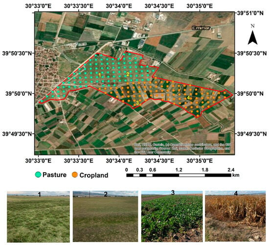
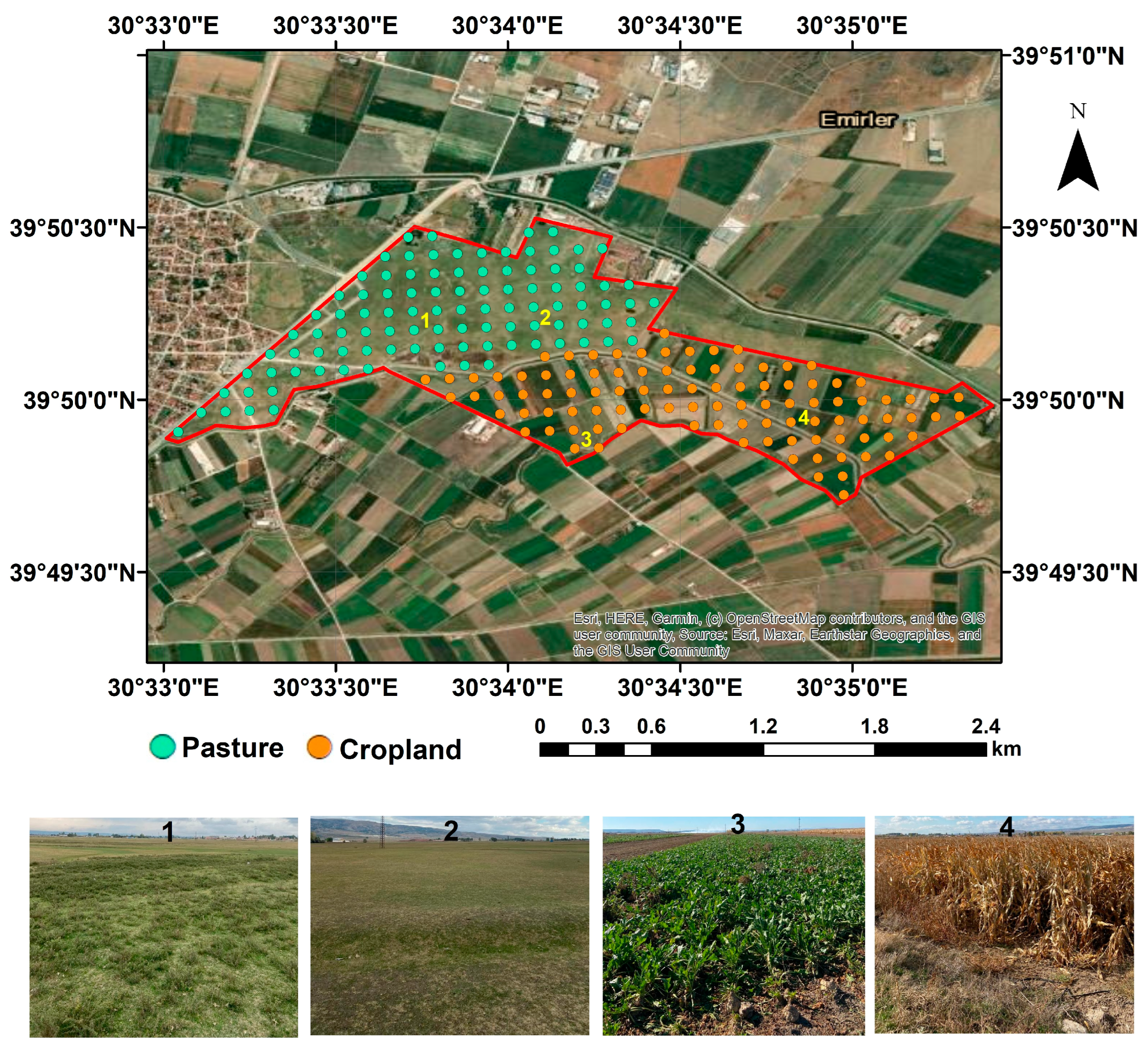
The study area is located in Eskisehir, Türkiye, in the Central Anatolia Region (Figure 1). The Köppen-Geiger climate classification of the research area is cold semi-arid (BSk), with an average annual temperature of 11.3 °C and an average annual precipitation of 372.9 mm. The Newhall model classified the soil moisture and temperature regimes as mesic and xeric (dry xeric in the subclass). The parent material is alluvial across the study area. Soil type was classified as Typic Rhodoxeralfs according to the US Soil Taxonomy [43]. The major horizons of this soil type were described as A1, A2, Bt, C1, and C2 [27]. The study area is characterized by almost flat slopes (0.5–1%) and an elevation range of 782–786 m a.s.l. In particular, the research area has a gentle slope from south to north. Soil samples (n = 200) were collected from pasture (n = 100) and cropland (n = 100) using a regular 100 m × 100 m sampling grid. The pasture areas are covered with natural vegetation, and the main crops in the cropland areas are corn, alfalfa, sugar beets, and wheat. Based on satellite imagery dating back to 1984, these areas have been used as pasture and cropland for more than 42 years. Soil samples were collected from 0 to 20 cm using a 7 cm Edelman auger. All soil samples were air-dried at room temperature and sieved in the laboratory using a sieve with a mesh size of <2 mm prior to physical and chemical analyses and soil spectral signatures.
Figure 1.
Location of the study site in Eskişehir, Türkiye. Teal (pasture) and orange (cropland) points show soil sampling locations (n = 200) based on a 100 × 100 m grid sampling design. The numbered areas (1–4) represent different land-use types and vegetation conditions, as illustrated in the photographs. Cropland areas (3 and 4) were cultivated with corn, alfalfa, and sugar beet, whereas pasture areas (1 and 2) are covered by natural vegetation. All photographs were taken in August 2022 (Red polygon represents the border of the study area).
The sand, silt, and clay contents were determined by the hydrometer method [44]. Soil pH and electrical conductivity (EC) were measured using a digital Isolab pH-EC meter (Isolab Inc., Eschau, Germany) in a 1:2.5 soil-to-water solution, with EC values corrected to 25 °C [43]. The CaCO3 content was determined by a Scheibler calcimeter [45]. Soil organic matter (SOM) was measured by the modified Walkley-Black method [46]. The SOC content was derived from the SOM content using the Van Bemmelen factor (1.724) [47].
2.2. Vis-NIR Scanning
Air-dried, ground, and sieved (2 mm) soil samples were used for Vis-NIR scanning. The soil spectrum for each soil sample was obtained using a portable ASD Field Spec 4 Vis-NIR spectrometer (Analytical Spectral Devices, Inc., Longmont, CO, USA), covering 350–2500 nm. The spectrometer has three detectors: (a) a 512-element silicon photodiode array that measures the spectral range of 350–1000 nm (3 nm resolution); (b) a 256-element InGaAs array that covers the spectral range of 1000–1900 nm (8 nm resolution); and (c) a 256-element InGaAs array that covers the spectral range of 1900–2500 nm (6 nm resolution). The Vis-NIR spectrometer was calibrated before the first scan and after every ten samples with a white reference plate (Labsphere, Inc., North Sutton, NH, USA). Three scans were obtained per soil sample, and these were averaged to create a single spectrum per sample. The raw spectrum comprised 2151 spectral points across the Vis-NIR range.
2.3. MIR Scanning
Before MIR scanning, air-dried, ground, and sieved (2 mm) soil samples were finely ground using a ball mill (Retsch Mixer Mill MM301, Verder Scientific GmbH & Co. KG, Haan, Germany). The 5 cm3 sieved (<2 mm) soil sample was placed into a 25 mL stainless steel milling cup with five 10 mm grinding balls. The samples were milled for 15 min at 25 Hz. MIR spectra were collected using a Bruker Alpha II benchtop spectrometer (Bruker Optik GmbH, Ettlingen, Germany) with a front-reflectance module. Absorbance values were 4050–550 cm−1, 64 co-scans, and a resolution of 4 cm−1. The MIR spectrometer was calibrated using a gold mirror reference before each soil sample was scanned. Each sample was scanned 4 times with a finely ground soil sample. The mean spectrum was obtained by averaging the four replicates. The raw MIR spectrum contains 1705 spectral points.
2.4. pXRF Scanning
Air-dried, ground, and sieved (2 mm) soil samples were scanned using a pXRF spectrometer (Hitachi, X-MET8000 Geo, Tokyo, Japan) at an energy range of 0–45 keV for 60 s to obtain soil spectra in Geochem Mode. The measurements were performed by placing the pXRF directly in contact with the soil sample surface. The pXRF spectroradiometer was calibrated using 316 stainless steel prior to scanning. No additional calibration was performed during the scanning of the 200 samples. As a result of these processes, 2048 spectral points were obtained across the pXRF spectra.
2.5. Spectral Preprocessing
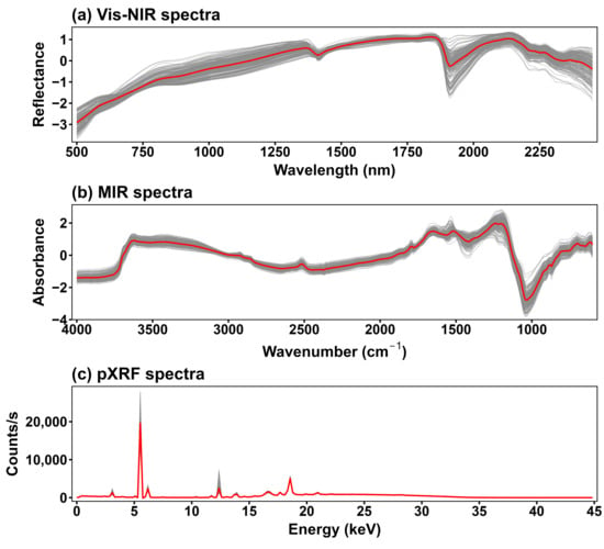
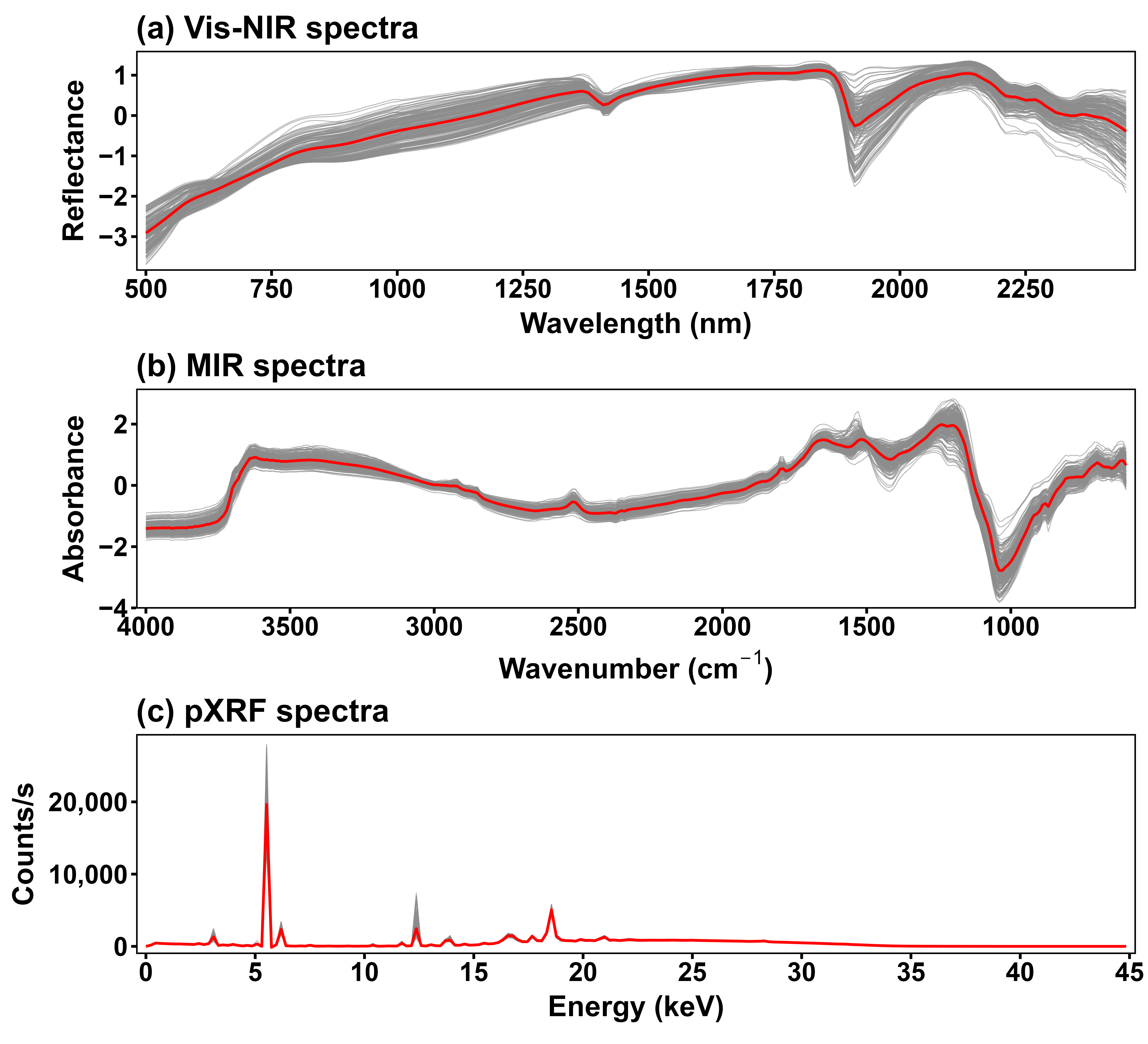
The following preprocessing steps were applied for Vis-NIR, MIR and pXRF spectra using the prospectr package [48] in R version 4.2.0 [49]: (i) smoothing of the spectra by the Savitzky–Golay filter [50] using a window size of 13 and a polynomial order of 2; (ii) removal of spectral regions between 350 and 499 nm and 2451–2500 nm for Vis-NIR and 4050–4001 cm−1 and 550–599 cm−1 to reduce noise; (iii) resampling of every tenth spectral point to minimize the effects of light scattering and baseline shift. After preprocessing of the Vis-NIR, MIR, and pXRF spectra, the number of variables derived from individual and combined spectral data was determined (Table 1), following the approach previously described in [51]. Figure 2 shows the spectral data obtained after preprocessing.
Table 1.
Predictor types, spectral points, and the number of variables used in each model under different sampling strategies. The number of variables derived from spectral data was determined after the preprocessing of Vis–NIR, MIR, and pXRF spectra.
Figure 2.
Vis-NIR (a), MIR (b), and pXRF (c) spectra of soil samples (n = 200). The spectral data shown were obtained after preprocessing. Gray lines represent individual spectra, whereas the red line indicates the mean spectrum calculated across all samples. The Vis-NIR spectra are shown as reflectance (500–2500 nm), MIR spectra as absorbance (4000–600 cm−1), and pXRF spectra as counts per second (0–45 keV) (Vis-NIR–Visible near-infrared; MIR–mid-infrared; pXRF–portable X-ray fluorescence).
2.6. Calibration Sample Selection Strategies
Four calibration sample selection strategies were applied: random sampling (RS), Kennard–Stone (KS), conditioned Latin Hypercube sampling (cLHS), and k-means clustering. Before principal component analysis (PCA), the complete dataset was randomly divided into a candidate calibration set (70%, n = 140) and a validation dataset (30%, n = 60). The validation dataset (n = 60) was kept fixed and was not included in PCA and sample selection. This design allowed all sampling strategies to be compared using the same validation dataset. From the 140 candidate samples, 100 samples were selected by each sampling strategy for model calibration. Thus, all models had the same number of calibration (n = 100) and were evaluated using the same validation samples (n = 60). PCA was applied separately to the 140 candidate samples for each individual (Vis-NIR, MIR, and pXRF) and combined spectral dataset (Vis-NIR + MIR, Vis-NIR + pXRF, MIR + pXRF, and Vis-NIR + MIR + pXRF) (Table 1). Before PCA, the variables in the combined spectral datasets were mean-centered and scaled to unit variance. PCs explaining 99% of the total spectral variance were retained. The resulting PCA scores were used for sample selection. PCA was used to reduce the number of spectral variables while retaining most of the spectral variation. Soil properties were not used for sample selection.
For RS, 100 samples were randomly selected from the 140 candidate calibration samples using the PCA scores. No additional criterion was used to select the samples. For KS, 100 samples were selected from the same candidate calibration dataset using the kenStone() function from the prospectr package. The method selects samples based on their distances in the PCA score space to obtain good coverage of the spectral variation. For cLHS, we used the clhs() function from the clhs package to select a subset of the samples that best represent the multivariate distribution of the spectral data. This method aims to retain the statistical properties of the original dataset by ensuring that the selected samples span the full range of variability across all variables. The cLHS method was also used to select 100 calibration samples. The base R kmeans() function was used to perform k-means clustering to group samples with similar spectral characteristics into clusters. The spectral data (represented by PC scores) were partitioned into a predefined number of clusters, and samples were selected proportionally from each cluster to form the calibration dataset. For consistency, 100 calibration samples were selected using this approach as well.
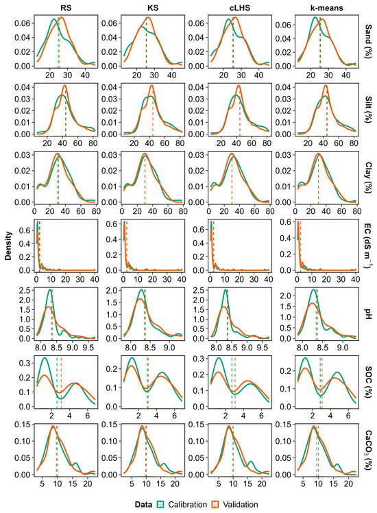
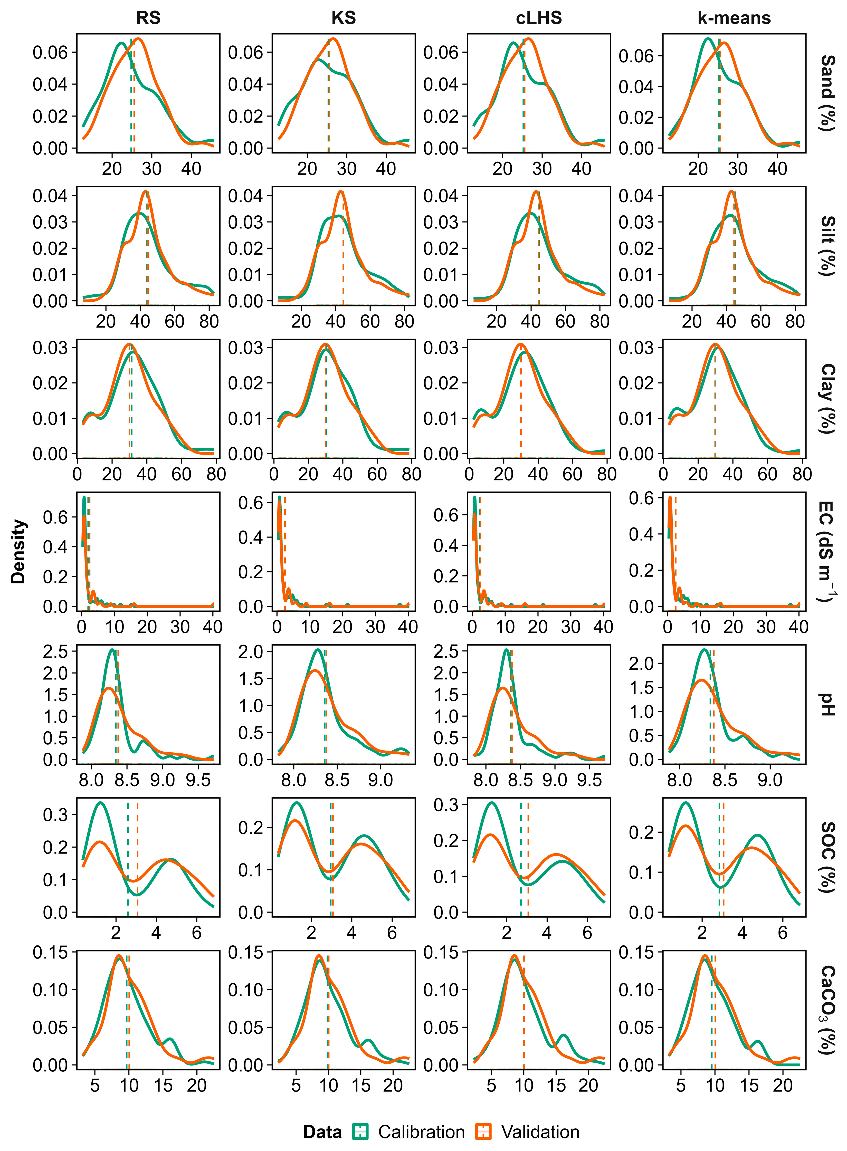
The same independent validation dataset (n = 60) was used to evaluate all prediction models regardless of the calibration sample selection strategy. Figure 3 shows the distribution of soil properties in the calibration datasets selected using MIR PCA scores and in the fixed validation dataset. Sample selection was based on spectral PCA scores because the aim was to select calibration samples according to spectral variability. Measured soil properties were therefore not included in the sample selection process. However, good representation of spectral variation may not always ensure full coverage of the range of each soil property, particularly for extreme values.
Figure 3.
Distribution patterns of soil properties under different sampling strategies (RS, KS, cLHS, and k-means) for calibration and validation datasets. Solid curves represent density distributions, whereas dashed lines indicate mean values. Calibration and validation subsets were selected based on MIR spectra, as they yielded superior individual-prediction performance compared to Vis–NIR and pXRF (EC–Electrical conductivity; SOC–Soil organic carbon; RS–Random sampling; KS–Kennard–Stone sampling; cLHS–Conditioned Latin hypercube sampling).
2.7. Machine Learning Models and Statistical Analyses
The complete dataset was first divided into calibration (70%) and validation (30%) subsets. For each calibration sample selection strategy (RS, KS, cLHS, and k-means), 100 representative samples were selected from the calibration dataset and used to train prediction models. Cubist and partial least squares regression (PLSR) were used to predict soil properties (sand, silt, clay, EC, pH, SOC, and CaCO3) using individual and combined spectra. Within each calibration dataset, repeated 10-fold cross-validation (10 repetitions) was used only for model training and hyperparameter tuning. For Cubist, the model was constructed using the M5 model tree approach, in which each rule was coupled with a linear regression model rather than a discrete value. The tuning parameters were tuned automatically during model training using the caret package. A maximum of 30 components was evaluated for PLSR, and the optimal number of components was selected based on the lowest RMSE. For the RF model, hyperparameters were also optimized automatically during model training. These hyperparameters for the cubist and PLSR models can be found in Supplementary Tables S1–S7. The final model performance was evaluated using the same independent validation dataset for all calibration sample selection strategies. Model performance was assessed using R2, RMSE, RPD, and RPIQ. These accuracy metrics were calculated for the calibration and validation datasets and can be found in Supplementary Tables S1–S7.
Variable importance was calculated using the varImp() function in the R caret package. For Cubist, importance was derived from the contribution of predictors to the model rules and linear models, whereas for PLSR, it was based on the weighted absolute regression coefficients. The resulting importance values were used to identify the most influential MIR wavenumbers for each soil property. Descriptive statistics of each soil property were calculated using the psych package [52] in R version 4.2.0 [49]. A Tukey comparison test at p < 0.05, using the agricolae package in R version 4.2.0 [49], was used to test the effects of land uses on each soil property. PCA was performed using the factoextra package [53] to illustrate group separation at the 95% confidence level. Pearson correlation coefficients (r) between soil properties and soil spectra (Vis-NIR, MIR, and pXRF) were computed with the stats package in R (version 4.2.0, R Core Team, 2022).
3. Results
3.1. Descriptive Statistics of Soil Properties
Table 2 presents descriptive statistics for sand, silt, clay, EC, pH, SOC, and CaCO3. Sand, silt, and clay contents ranged from 12.62% to 45.84%, 6.54% to 82.78%, and 2.44% to 78.62%, respectively. Their coefficients of variation (CV) were 25.55%, 30.22%, and 47.41%. EC ranged from 0.35 to 40.33 dS m−1 with a CV of 196.28%. Soil pH varied from 7.82 to 9.72 with a CV of 3.45%. SOC ranged from 0.61% to 11.81% with a CV of 64.71%. CaCO3 contents ranged from 2.23% to 22.51% with a CV of 34.51%. The CV was highest for EC at 196.3, followed by SOC and clay at 64.7 and 47.4, respectively.
Table 2.
Descriptive statistics of the dataset used in the prediction models.
3.2. Effect of Land Use on Soil Properties
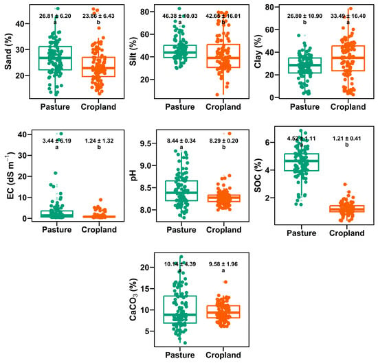
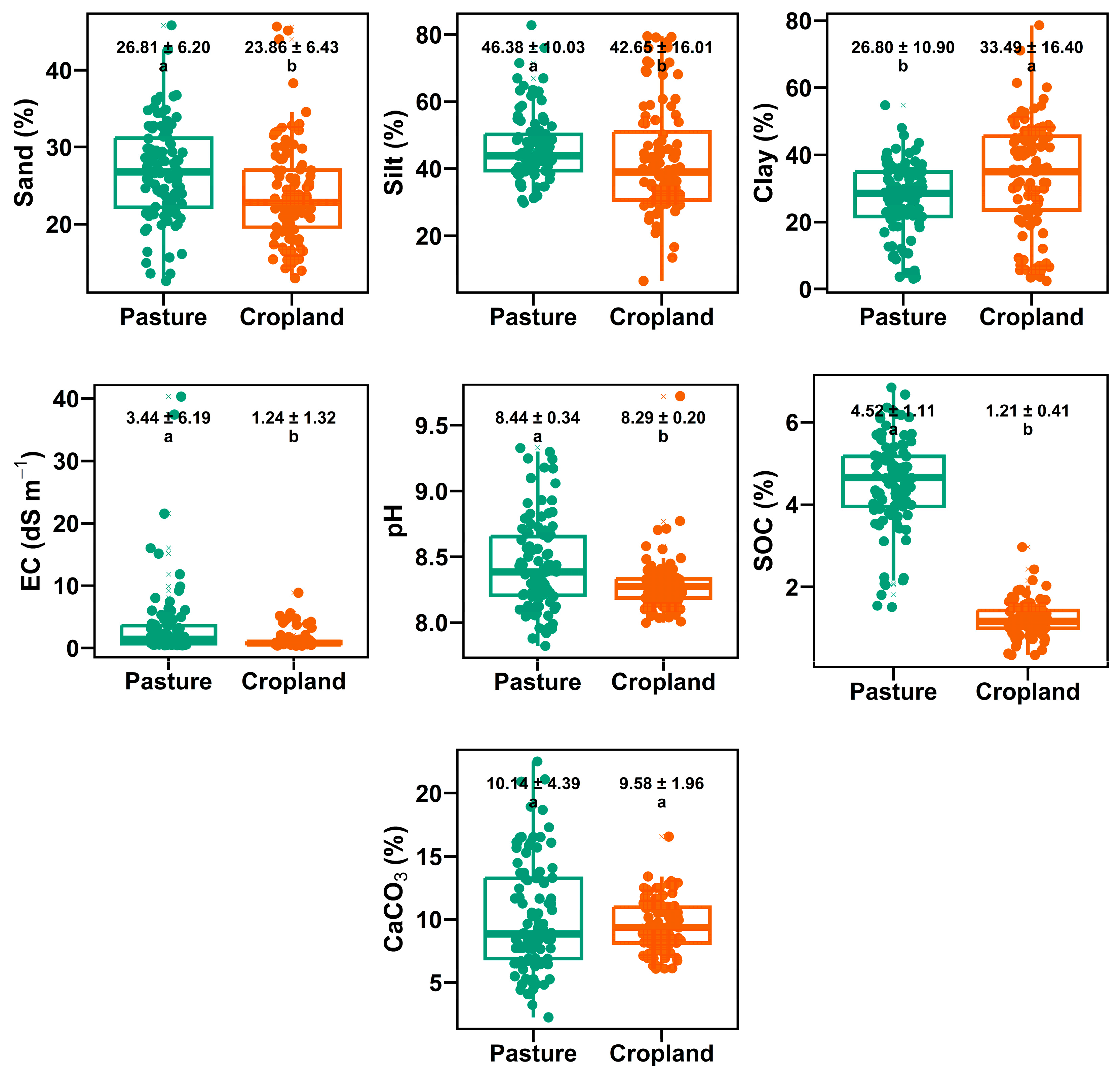
The variations in soil properties under pasture and cropland are presented in Figure 4. Significant differences (p < 0.05) between pasture and cropland were observed for all soil properties, except CaCO3. Sand content was higher in pasture (26.81%) than in cropland (23.86%), while silt content was also higher in pasture (46.38%) compared to cropland (42.65%). In contrast, clay content was higher in cropland (33.49%) than in pasture (26.80%). EC was higher in pasture (3.44 dS m−1) than in cropland (1.24 dS m−1). Soil pH was slightly higher in pasture (8.44) than in cropland (8.29). SOC showed higher values in pasture (4.52%) than in cropland (1.21%). CaCO3 values were similar between pasture (10.14%) and cropland (9.58%).
Figure 4.
Variation in soil properties under different land-use types (pasture and cropland). Values above each box represent mean ± standard deviation. Different letters indicate significant differences between land-use types based on Tukey’s test (p < 0.05). Box plots show the median (line), interquartile range (box), and minimum and maximum values (whiskers), with outliers indicated by points. (EC–Electrical conductivity; SOC–Soil organic carbon).
3.3. Pearson Correlation Between Soil Properties and Vis-NIR, MIR, and pXRF Spectra
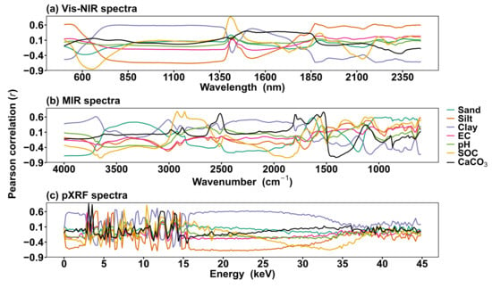
The patterns of Pearson correlation (r) between soil properties and soil spectral points in Vis-NIR, MIR, and pXRF are shown in Figure 5. Clay, SOC and CaCO3 had relatively stronger correlations in the Vis–NIR region compared with sand, silt and EC. The highest positive Pearson correlation (r = 0.87) was observed between Vis-NIR and SOC at 1410 nm, whereas CaCO3 was highly negatively correlated (r = −0.85) with Vis-NIR spectra. In the Vis-NIR spectral region, soil properties had higher positive and negative values in the 770–1370 nm and 1870–2450 nm ranges, which generally had a strong and stable impact on the Pearson correlation, whereas the other parts of Vis-NIR had no stable correlations between soil properties and Vis-NIR spectra.
Figure 5.
Pearson correlation (r) patterns between spectral variables and soil properties across Vis-NIR (a), MIR (b), and pXRF (c) spectra. Lines represent individual soil properties (sand, silt, clay, EC, pH, SOC, and CaCO3), highlighting spectral regions associated with their variability (EC–Electrical conductivity; SOC–Soil organic carbon; Vis-NIR–Visible near-infrared; MIR–mid-infrared; pXRF–portable X-ray fluorescence).
In the MIR region, the highest correlations were observed for SOC, CaCO3, and clay. These properties were more strongly associated with MIR spectral features. Correlations were relatively weak for sand and silt. The maximum positive and negative Pearson correlation coefficients (r = 0.78 and r = −0.74) were observed between MIR and SOC at 2920 and 3660 cm−1, respectively. Calcium carbonate was positively correlated to 3.09 keV (r = 0.86) and silt was negatively correlated to 11.71 keV (r = −0.69) in the pXRF spectra. The correlation pattern of soil properties showed abrupt changes in the 0–15 keV and 35–45 keV ranges. A more stable correlation pattern was observed between 15 and 35 keV.
3.4. Prediction of Soil Properties Based on Sampling Strategies and Spectrometers
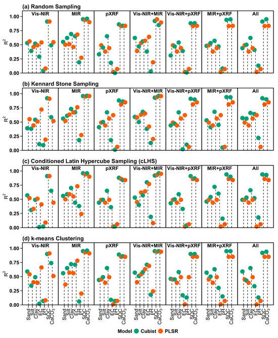
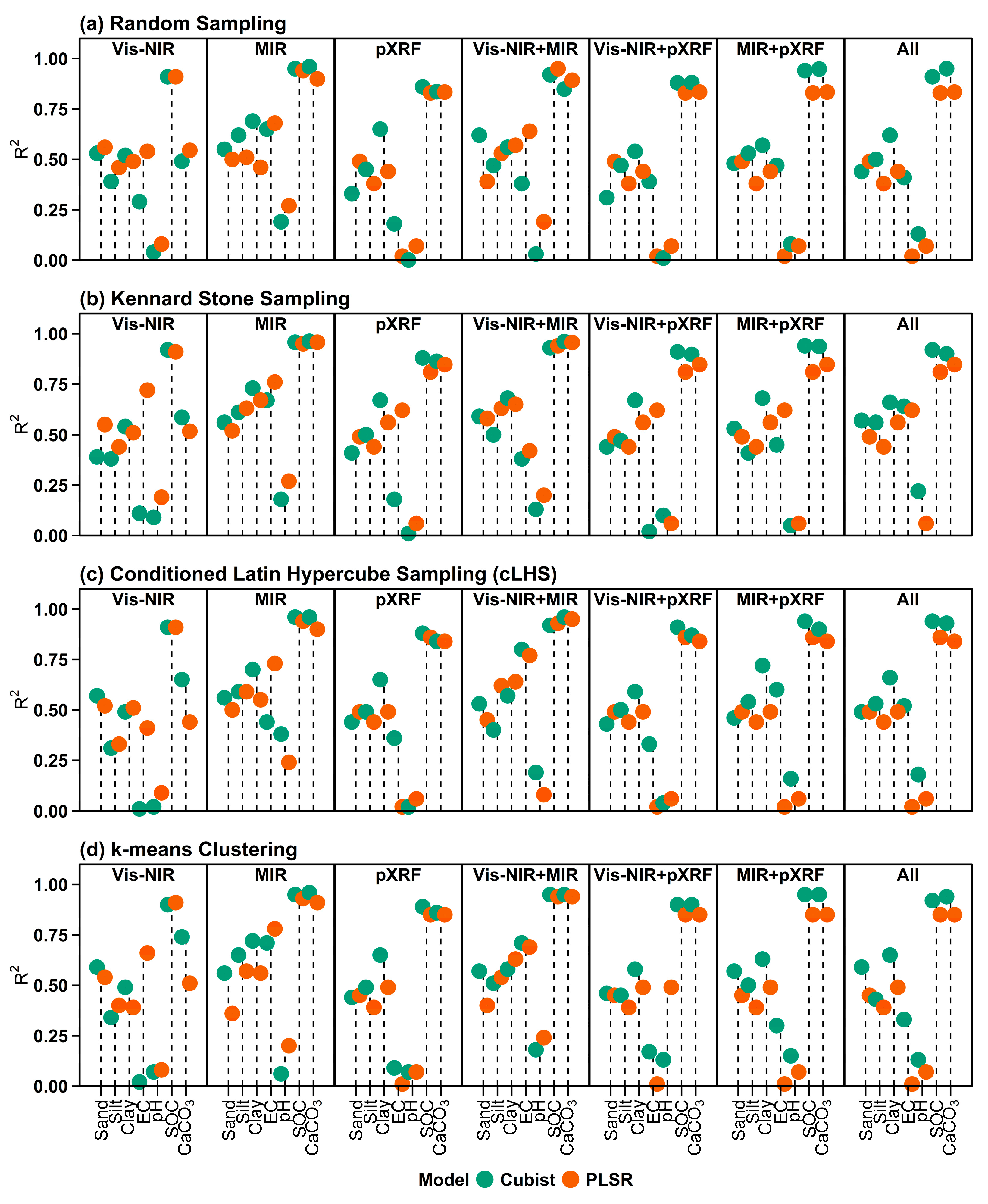
Figure 6 presents the prediction accuracies (R2) of the Cubist and PLSR models for soil properties, using individual and combined spectral datasets across different sampling strategies, including validation results. The other prediction accuracy metrics, such as RMSE, RPD, and RPIQ, can be found in Supplementary Tables S1–S7. Detailed results for each sampling model, spectra, and soil properties, based on calibration and validation using accuracy metrics such as R2, RMSE, RPD, and RPIQ, are provided in Supplementary Tables S1–S7.
Figure 6.
Prediction accuracy (R2) of Cubist and PLSR models for soil properties using individual (Vis-NIR, MIR, and pXRF) and combined spectral datasets under different sampling strategies. “All” represents the combination of all spectral data sources (Vis-NIR + MIR + pXRF) (EC–Electrical conductivity; SOC–Soil organic carbon; Vis-NIR–Visible near-infrared; MIR–Mid-infrared; pXRF–Portable X-ray fluorescence; PLSR–Partial least squares regression).
In terms of RS (Figure 6a), MIR produced higher prediction accuracy (R2) values than Vis-NIR and pXRF for most soil properties. In particular, SOC (R2 = 0.96, RMSE = 0.71, RPD = 4.78, and RPIQ = 8.65) and CaCO3 (R2 = 0.96, RMSE = 0.69, RPD = 5.07, and RPIQ = 5.09) had higher prediction accuracy using MIR spectra with the Cubist model. Vis-NIR showed moderate prediction accuracy, whereas pXRF yielded lower accuracy, particularly for EC and SOC. The combination of spectral datasets (Vis-NIR + MIR) produced moderate prediction accuracy for sand (R2 = 0.62, RMSE = 3.49, RPD = 1.63, and RPIQ = 2.07). Cubist slightly outperformed PLSR in most spectral models.
For the KS strategy (Figure 6b), prediction accuracy was generally higher for EC (R2 = 0.76, RMSE = 2.75, RPD = 2.02, and RPIQ = 0.45), SOC, CaCO3, and clay, and was more stable than that for RS. MIR achieved higher prediction accuracy for EC, SOC, sand, silt, and clay than Vis-NIR and pXRF spectra. However, the individual use of Vis-NIR and pXRF achieved moderate prediction accuracy for soil properties. Combined datasets (Vis-NIR + MIR) achieved the highest accuracy for CaCO3 and sand, with R2 values ranging from 0.39 to 0.96 (RMSE = 0.71–5.35, RPD = 1.06–4.97, and RPIQ = 1.35–4.98). EC, pH, and silt achieved higher prediction accuracy with the PLSR model, whereas SOC, CaCO3, sand, and clay were better predicted by the Cubist model.
In the conditioned Latin hypercube sampling (cLHS) approach (Figure 6c), prediction performance remained high for MIR spectra of SOC (R2 = 0.96, RMSE = 3.49, RPD = 1.63, and RPIQ = 2.07), followed by CaCO3 (R2 = 0.96, RMSE = 0.72, RPD = 4.85, and RPIQ = 4.87) compared to Vis-NIR and pXRF spectra. However, when using combined spectra (Vis-NIR + MIR and Vis-NIR + pXRF), the prediction accuracies for EC (R2 = 0.80, RMSE = 3.12, RPD = 1.78, and RPIQ = 0.40), silt (R2 = 0.62, RMSE = 7.97, RPD = 1.58, and RPIQ = 1.53), and clay (R2 = 0.72, RMSE = 7.35, RPD = 1.87, and RPIQ = 2.14) were improved. Silt achieved higher prediction accuracy with the PLSR model, whereas other soil properties were better predicted by the Cubist model.
For k-means clustering (Figure 6d), when considering individual performance, MIR achieved higher prediction accuracy for EC, CaCO3, silt and clay, whereas sand was moderately predicted by Vis-NIR spectra. SOC and pH showed higher prediction accuracy when using combined spectra (Vis-NIR + pXRF and MIR + pXRF). Vis-NIR showed moderate performance, whereas pXRF alone yielded lower accuracy. The PLSR model had higher prediction accuracy for EC and pH, whereas the Cubist model performed better for CaCO3, SOC, sand, silt, and clay.
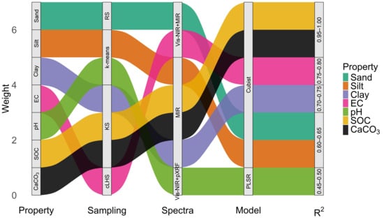
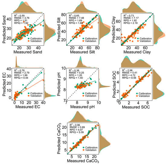
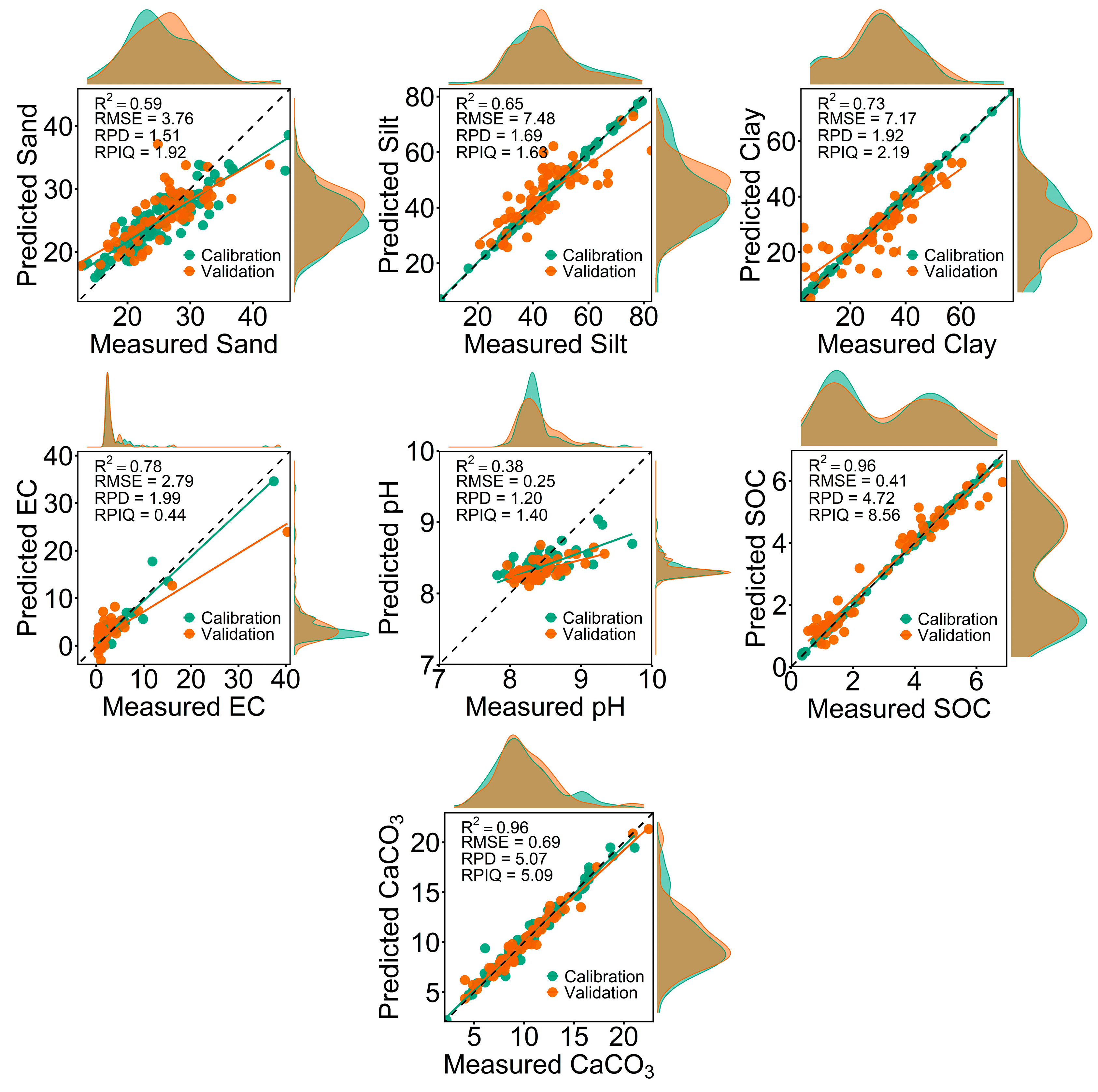
Overall, for individual use of a spectrometer (Vis-NIR, MIR, or pXRF), soil properties, along with sampling strategies, were better predicted by MIR spectra than by Vis-NIR or pXRF spectra (Figure 7). Therefore, scatterplots of measured versus predicted values obtained from MIR spectra for each soil property are presented in Figure 8. When spectral sources were used together, Vis-NIR contributed more to MIR prediction performance than pXRF. For instance, in terms of the best prediction performance, SOC (R2 = 0.96, RMSE = 0.41, RPD = 4.72, and RPIQ = 8.56, KS, Cubist), silt (R2 = 0.65, RMSE = 7.48, RPD = 1.69, and RPIQ = 1.63, k-means, Cubist), clay (R2 = 0.73, RMSE = 7.17, RPD = 1.92, and RPIQ = 2.19, KS, Cubist), and CaCO3 (R2 = 0.96, RMSE = 0.69, RPD = 5.07, and RPIQ = 5.09, KS, Cubist) were the most accurately predicted properties using MIR spectra. Sand (R2 = 0.62, RMSE = 3.49, RPD = 1.63, and RPIQ = 2.07, RS, Cubist) and EC (R2 = 0.80, RMSE = 3.12, RPD = 1.78, and RPIQ = 0.40, cLHS, Cubist) were well predicted by combined Vis-NIR and MIR spectra, whereas pH obtained higher prediction accuracy (R2 = 0.49, RMSE = 10.04, RPD = 1.37, and RPIQ = 1.56, k-means, PLSR) using Vis-NIR + pXRF spectra (Figure 8).
Figure 7.
Sankey diagram showing the optimal combinations of calibration model, spectral dataset, and modeling approach for predicting soil properties, along with their corresponding R2 values. Flow widths indicate the relative contribution (weight) of each pathway (EC–Electrical conductivity; SOC–Soil organic carbon; RS–Random sampling; KS–Kennard-Stone sampling; cLHS–Conditioned Latin hypercube sampling; Vis-NIR–Visible near-infrared; MIR–Mid-infrared; pXRF–Portable X-ray fluorescence).
Figure 8.
Scatterplots of measured versus predicted values of soil properties using MIR spectra, selected due to their superior prediction performance compared to Vis-NIR and pXRF spectra. The dashed line represents the 1:1 relationship, and solid lines indicate regression fits for calibration and validation datasets (EC–Electrical conductivity; SOC–Soil organic carbon).
3.5. Variable Importance of Models
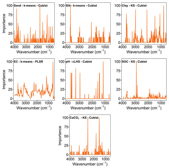
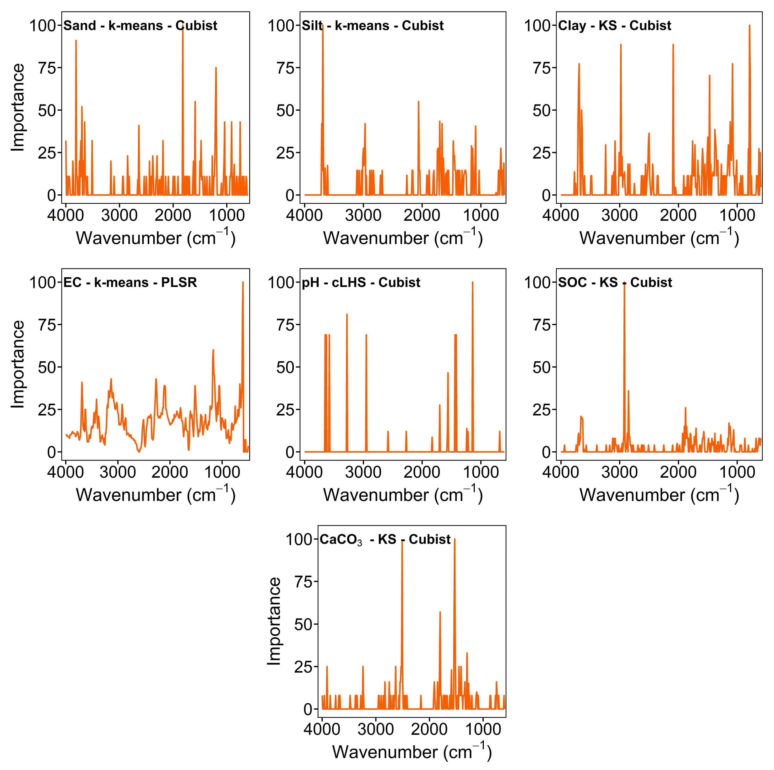
When comparing individual use of the spectrometer, MIR achieved higher prediction accuracy for each soil property. Therefore, the variable importance distributions across MIR wavenumbers for the best-performing model and sampling combinations are shown in Figure 8. The results showed that the importance of spectral regions or points varied based on soil properties. For PLSR, the variable importance patterns of silt and clay were similar. Other soil properties, including sand, EC, pH, SOC, and CaCO3, were well predicted with the Cubist model.
For each soil property, the three most important MIR wavenumbers that contributed to the model prediction were identified. For sand, the most influential points were 1820, 3810, and 1200 cm−1. The dominant wavenumbers for silt were 3690, 2060, and 1700 cm−1, and for clay were 790, 2980, and 2090 cm−1. The most important spectral regions for EC were 600, 610, and 1170 cm−1. The main factors for pH are also at wavenumbers 1140, 3280, and 3650 cm−1. SOC was mainly dominated by 2920, 2850, and 1880 cm−1, while CaCO3 was mainly controlled by 1530, 2510, and 1800 cm−1 (Figure 9).
Figure 9.
Variable importance for Cubist and PLSR across MIR wavenumbers for predicting soil properties. Each panel represents the best-performing combination of soil property, sampling strategy, and model (EC–Electrical conductivity; SOC–Soil organic carbon; RS–Random sampling; KS–Kennard–Stone sampling; cLHS–Conditioned Latin hypercube sampling).
3.6. Variability in Prediction Accuracy Across Calibration Sample Selection Strategies
The variability in prediction accuracy among the four calibration sample selection strategies differed across soil properties, sensors, and models (Table 3). EC showed the largest variability overall, with R2 differences ranging from 0.10 to 0.61. The highest difference (0.61) was observed for pXRF, Vis-NIR + pXRF, MIR + pXRF, and All spectra when using PLSR. In contrast, EC variability was lower for MIR with PLSR (0.10).
Table 3.
Variability in soil property prediction accuracy across calibration sample selection strategies for different sensors and models.
The effect of calibration sample selection was generally smaller for SOC than for the other soil properties. Differences in R2 ranged from 0 to 0.05 across all sensor-model combinations. No difference was observed for SOC using Vis-NIR with PLSR, while the largest difference was 0.05 for several pXRF-based combinations. CaCO3 also showed relatively low variability in most cases, although larger differences were observed for Vis-NIR (0.25) and pXRF (0.12) with Cubist. For the particle-size fractions, variability was generally moderate. Sand showed R2 differences ranging from 0.01 to 0.20, with the largest difference observed for Vis-NIR with Cubist. Silt ranged from 0.05 to 0.13, whereas clay ranged from 0.02 to 0.21. The highest variability for clay was obtained with MIR using PLSR. The variability in pH predictions depended strongly on the sensor-model combination. Differences were low for pXRF, MIR + pXRF, and all spectra with PLSR (0.01), but increased to 0.32 for MIR with Cubist and 0.43 for Vis-NIR + pXRF with PLSR. Overall, the results show that the influence of calibration sample selection on prediction accuracy was property-dependent, with the largest differences generally observed for EC and the smallest for SOC.
4. Discussion
4.1. Land Use
The results showed significant (p < 0.05) differences between cropland and pasture soils, except for CaCO3. Sand and silt contents were higher in the pasture, whereas clay content was higher in the cropland areas. This can be related to long-term tillage practices. For instance, regular tillage and plowing break down soil aggregates and trigger soil formation, which can lead to the accumulation of clay in cropland areas. In contrast, the soils are undisturbed and protected by vegetation, which helps maintain a more balanced structure in the pasture areas. Similarly, Tamene et al. [54] reported similar changes after long-term cultivation.
EC was higher in pasture than in cropland areas. This may be associated with heavy grazing activity in the pasture areas. As animals return nutrients to the soil through manure and urine. This can lead to higher soluble salt concentrations and EC values. Grazing systems also tend to retain nutrients in the soil, whereas cropland often loses them through harvest and leaching. For example, Qu et al. [55] reported that grazing increased EC due to salt accumulation and changes in soil conditions. Similarly, grazing has been shown to alter soil chemical properties and nutrient distribution, thereby contributing to higher EC levels [56]. These changes are closely linked to nutrient cycling processes in grazed systems [57].
Soil pH is slightly higher in the pasture than in the cropland soils, and both soils were alkaline. This can be explained by land management and biological processes. For instance, in pasture areas, grazing can increase soil pH by returning basic cations from manure and urine. These inputs can lead to a gradual increase in soil alkalinity [55]. In addition, agricultural practices such as fertilization, especially the use of ammonium-based fertilizers, can lead to slight soil acidification over time [58,59,60]. These processes may explain the relatively lower pH observed in the cropland. Similarly, Qu et al. [55] compared soil pH between cropland and pasture soils and reported a relatively lower soil pH in cropland than in pasture soils.
The pasture soils had higher SOC than the cropland soils. The higher SOC in the pasture soils can be related to plant cover, root biomass, and slower decomposition rates under undisturbed conditions. In cropland, lower SOC may be associated with tillage, which breaks soil aggregates and exposes organic matter, initiating decomposition [61,62]. It can also be related to reduced organic inputs and faster mineralization [63].
CaCO3 contents did not show a significant difference between the pasture and cropland soils. This can be related to similar parent material across the study area. Adding CaCO3 is commonly used to increase soil pH in acidic conditions. However, it is not typically applied in alkaline agricultural soils. Therefore, variations in CaCO3 contents are mainly controlled by long-term soil-forming processes rather than by short-term land use [64].
4.2. Vis-NIR, MIR, and pXRF Spectrometers
The results showed that MIR spectra achieved the highest prediction accuracy for each soil property across all sampling strategies compared with the individual use of spectrometers. The higher prediction accuracy of MIR can be attributed to its sensitivity to fundamental molecular vibrations. MIR reflectance spectra can directly capture absorption features related to organic matter, carbonates, and clay minerals [11,12]. This knowledge explains why soil properties, in particular SOC and CaCO3, were well predicted in our study. Similar findings were reported by Naimi et al. [15] and Gozukara et al. [16], who found that MIR is more effective than Vis-NIR and pXRF spectra for predicting soil properties due to its direct interaction with soil constituents.
Vis-NIR spectra showed moderate prediction accuracy for most soil properties compared to MIR and pXRF spectra. Vis-NIR measures overtones and combinations of molecular vibrations rather than fundamental absorptions [5]. As a result, the signal is weaker and more susceptible to external factors, such as masking by other soil properties (e.g., SOC, CaCO3), soil color, and surface conditions. Despite this limitation, combined Vis-NIR and MIR spectra obtained relatively higher prediction accuracy for sand, silt, EC, and CaCO3 across calibration sample selection in our study. These improvements in the prediction accuracy of EC and CaCO3 may be related to soil color and iron-related features that are not fully captured by MIR. Soil color is influenced by a number of soil properties including organic matter, iron oxides and carbonates [5,9]. Thus, Simon et al. [65] used the range of 360 to 830 nm to obtain soil color coordinates such as RGB, HSV, and CIE L*a*b*, and reported that these coordinates are useful for characterizing soils. Previous studies obtained higher prediction accuracy when using combined Vis-NIR and MIR spectra. These sensors offer complementary information on soil properties [5,6].
The prediction accuracy of pXRF was relatively lower than Vis-NIR and MIR spectra. The lower performance of pXRF may be related to its measurement of elemental concentrations rather than molecular structures [13]. Hence, it has limited sensitivity to properties such as SOC and EC. However, pXRF may provide useful information on mineral-related properties such as CaCO3. It shows elements related to carbonates, especially Ca [13]. This study improved the prediction accuracy for CaCO3 by combining MIR and pXRF. Thus, the fusion of molecular and elemental information can improve prediction performance [5,6].
Another important finding is the difference between the prediction models (Cubist and PLSR) modeling approaches. In terms of best results, the Cubist model achieved higher prediction accuracy for sand, silt, clay, EC, SOC, and CaCO3, whereas the PLSR model achieved higher prediction accuracy for pH. This can be explained by the models’ capabilities. Cubist can capture nonlinear relationships and interactions among variables, whereas PLSR is more suitable for linear relationships and works well when spectral responses are consistent [66,67].
4.3. Sampling Strategies
Sampling strategy affected the prediction accuracy of soil properties. The results showed that KS, cLHS, and k-means sampling strategies generally achieved higher prediction accuracy for sand (Vis-NIR + MIR), silt (MIR), clay (MIR), EC (Vis-NIR + MIR), pH (Vis-NIR + pXRF), and SOC (MIR), whereas RS achieved better prediction accuracy for sand using combined Vis-NIR and MIR spectra.
The sampling strategy greatly affected the prediction accuracy for soil properties, as each method captures the dataset’s variability differently. Results from RS were generally lower and more variable; however, sand contents were well predicted using combined Vis-NIR and MIR spectra with the RS strategy. This is mainly because samples are chosen without considering the distribution of spectral space. Some important or extreme observations might not be part of the calibration set. If the dataset’s variability is not well represented, the model will not be able to learn the relationship between the spectra and the soil properties. This often leads to weaker and less robust predictions. Similarly, these limitations in RS were reported in previous soil spectroscopy studies [36,37,38]. Some studies performed better predictions using RS and individual or combined Vis-NIR, MIR and pXRF spectra of soil properties (i.e., SOC, sand, silt, clay) [7,15]. The higher accuracies reported in the studies may be attributed to differences in dataset variability such as sample size, properties, and spectral data. That is why the model learned to predict soil properties well.
In contrast, the KS strategy showed more stable and accurate prediction of clay, SOC, and CaCO3 using MIR spectra. The primary benefit of KS is that it samples points that are far apart in spectral space. This way, the calibration set covers the full range of spectral variability and redundancy between samples is minimized [41]. A more representative calibration set will allow the model to better describe common and extreme conditions in the dataset. This might be the reason why KS is better in predicting SOC and clay in this study. Similar results have been reported in previous studies for infrared spectroscopy, where KS provided representative calibration sets by improving the coverage of spectral variability [36]. However, the performance of KS may vary among soil properties and datasets. In our study, KS performed particularly well for clay, SOC, and CaCO3 using MIR spectra.
The cLHS method also performed well, especially for the prediction of EC. In this study, cLHS was applied to the spectral PCA scores to select samples representing the distribution of spectral variability. The method aimed to select representative samples while maintaining the statistical distribution of the input variables [68]. This may explain the relatively good performance of cLHS for some soil properties in this study.
The k-means method also yielded quite good results, particularly on the combined spectrum. This method groups similar samples and picks one sample as the representative of each group. Thus, the calibration set contains the main patterns in the dataset, thereby alleviating sample redundancy. The success of k-means depends on how well the clusters can capture the true variability of the soil data. If the clustering structure is not fully representative of soil variability, some important observations may be underrepresented. This may explain the somewhat lower performance of k-means compared to KS and cLHS for some soil properties.
Previous studies using Vis-NIR and MIR spectra have also shown that calibration sample selection can affect prediction performance [36,37,38,39,40]. They reported that the performance of RS, KS, cLHS, and clustering-based methods has been reported to vary depending on the soil property, dataset, and prediction model. Our results are generally consistent with these studies because no single sampling strategy performed best for all soil properties and spectral datasets. However, KS and cLHS generally provided higher prediction accuracy than RS for several soil properties in our dataset.
Compared with Vis-NIR and MIR, calibration sample selection has been less studied for pXRF data. Previous studies have mainly focused on Vis-NIR and MIR spectral data, while calibration sample selection based on pXRF spectral information remains limited. In this study, RS, KS, cLHS, and k-means were compared using pXRF data as well as its combinations with Vis-NIR and MIR. This provides further information on the use of calibration sampling strategies for pXRF and fused spectral datasets that include pXRF spectra.
Differences in soil properties between pasture and cropland may also affect spectral variability and calibration sample selection. Sampling strategies that better represent this variability may provide more representative calibration datasets. However, the models were developed using the combined dataset rather than separately for each land use. Therefore, the effect of land use on individual sampling strategies was not directly evaluated. Future studies could examine sampling strategies separately for different land-use types.
The validation set was randomly selected from the same study area and hence was not spatially independent. Therefore, the reported prediction performance could have been affected by possible spatial autocorrelation among calibration and validation samples. However, the present study was concerned with comparing calibration sample selection strategies using the same fixed validation dataset rather than evaluating spatial prediction or model transferability. Therefore, the reported prediction performance should be understood in relation to the study area. Future studies can further evaluate the transferability of the models with spatially independent validation data.
The study obtained spectra of laboratory-prepared soil samples under controlled conditions. Thus, the results may not directly reflect prediction performance under in situ field conditions. Soil moisture, surface roughness and aggregate structure can influence spectral measurements and model performance. Additional studies are necessary to assess the performance of these calibration sampling strategies under field conditions.
5. Conclusions
This study evaluated the influence of different calibration sample selection strategies on predicting key soil properties (sand, silt, clay, EC, pH, SOC, and CaCO3) using individual and combined Vis-NIR, MIR, and pXRF spectroscopy, and explored the effects of land-use differences on soil properties. The results clearly demonstrate that each soil property, except CaCO3, was significantly affected (p < 0.05) by land-use differences (pasture vs. cropland). Cropland soils had higher clay content, whereas pasture soils had higher sand, silt, EC, pH, SOC, and CaCO3. The calibration sample sampling selection strategy and the use of individual or combined spectral sources were decisive for predicting soil properties. KS, cLHS, and k-means clustering achieved higher prediction accuracy for silt, clay, EC, pH, SOC, and CaCO3, whereas RS performed well only for sand. Individual use of MIR outperformed Vis-NIR and pXRF in predicting soil properties. Combined spectra achieved higher accuracy for sand (Vis-NIR and MIR), EC (Vis-NIR and MIR), and pH (Vis-NIR + pXRF). The Cubist model generally performed better than PLSR. Results show that calibration sample selection had a greater effect on EC and pH, particularly in pXRF and fused spectral datasets. In contrast, SOC was consistently the least affected by calibration sample selection, whereas sand, silt, clay, and CaCO3 generally showed low to moderate variability across the different calibration sample selection strategies. These results show that the calibration sampling strategy was crucial for prediction accuracy, not only for individual spectra but also for combined spectra. This study provided practical guidance on optimizing calibration strategies and sample selection for future applications of individual and combined soil spectroscopy.
Supplementary Materials
The following supporting information can be downloaded at: https://www.mdpi.com/article/10.3390/agronomy16191911/s1, Table S1: Calibration and validation results of sampling strategies with Cubist and PLSR models used for predicting soil properties using Vis-NIR spectra; Table S2: Calibration and validation results of sampling strategies with Cubist and PLSR models used for predicting soil properties using MIR spectra; Table S3: Calibration and validation results of sampling strategies with Cubist and PLSR models used for predicting soil properties using pXRF spectra; Table S4: Calibration and validation results of sampling strategies with Cubist and PLSR models used for predicting soil properties using Vis-NIR + MIR spectra; Table S5: Calibration and validation results of sampling strategies with Cubist and PLSR models used for predicting soil properties using Vis-NIR + pXRF spectra; Table S6: Calibration and validation results of sampling strategies with Cubist and PLSR models used for predicting soil properties using MIR + pXRF spectra; Table S7: Calibration and validation results of sampling strategies with Cubist and PLSR models used for predicting soil properties using Vis-NIR + MIR + pXRF spectra;
Funding
This work has been supported by the Scientific and Technological Research Council of Türkiye (TÜBİTAK) under grant number 121O051.
Data Availability Statement
The raw data supporting the conclusions of this article will be made available by the author on request.
Conflicts of Interest
The author declares no conflicts of interest.
Abbreviations
The following abbreviations are used in this manuscript:
| Vis-NIR | Visible near-infrared |
| MIR | Mid-infrared |
| pXRF | Portable X-ray fluorescence |
| PLSR | Partial least square regression |
| SOC | Soil organic carbon |
| EC | Electrical conductivity |
| RS | Random sampling |
| KS | Kennard-Stone |
| cLHS | Conditioned Latin hypercube sampling |
References
- Gregory, A.S.; Ritz, K.; McGrath, S.P.; Quinton, J.N.; Goulding, K.W.T.; Jones, R.J.A.; Harris, J.A.; Bol, R.; Wallace, P.; Pilgrim, E.S.; et al. A review of the impacts of degradation threats on soil properties in the UK. Soil Use Manag. 2015, 31, 1–15. [Google Scholar] [CrossRef] [Scilit] [PubMed]
- Rabot, E.; Wiesmeier, M.; Schlüter, S.; Vogel, H.J. Soil structure as an indicator of soil functions: A review. Geoderma 2018, 314, 122–137. [Google Scholar] [CrossRef] [Scilit]
- Schröder, J.J.; Schulte, R.P.O.; Creamer, R.E.; Delgado, A.; Van Leeuwen, J.; Lehtinen, T.; Rutgers, M.; Spiegel, H.; Staes, J.; Tóth, G.; et al. The elusive role of soil quality in nutrient cycling: A review. Soil Use Manag. 2016, 32, 476–486. [Google Scholar] [CrossRef] [Scilit]
- Viscarra Rossel, R.A.; Behrens, T.; Ben-Dor, E.; Brown, D.J.; Demattê, J.A.M.; Shepherd, K.D.; Shi, Z.; Stenberg, B.; Stevens, A.; Adamchuk, V.; et al. A global spectral library to characterize the world’s soil. Earth-Sci. Rev. 2016, 155, 198–230. [Google Scholar] [CrossRef] [Scilit]
- Viscarra Rossel, R.A.; Walvoort, D.J.J.; McBratney, A.B.; Janik, L.J.; Skjemstad, J.O. Visible, near infrared, mid infrared or combined diffuse reflectance spectroscopy for simultaneous assessment of various soil properties. Geoderma 2006, 131, 59–75. [Google Scholar] [CrossRef] [Scilit]
- Nocita, M.; Stevens, A.; van Wesemael, B.; Aitkenhead, M.; Bachmann, M.; Barthès, B.; Ben Dor, E.; Brown, D.J.; Clairotte, M.; Csorba, A.; et al. Soil spectroscopy: An alternative to wet chemistry for soil monitoring. Adv. Agron. 2015, 132, 139–159. [Google Scholar] [CrossRef] [Scilit]
- O’Rourke, S.M.; Minasny, B.; Holden, N.M.; McBratney, A.B. Synergistic use of Vis-NIR, MIR, and XRF spectroscopy for the determination of soil geochemistry. Soil Sci. Soc. Am. J. 2016, 80, 888–899. [Google Scholar] [CrossRef] [Scilit]
- Xu, D.; Zhao, R.; Li, S.; Chen, S.; Jiang, Q.; Zhou, L.; Shi, Z. Multi-sensor fusion for the determination of several soil properties in the Yangtze River Delta, China. Eur. J. Soil Sci. 2019, 70, 162–173. [Google Scholar] [CrossRef] [Scilit]
- Stenberg, B.; Rossel, R.A.V.; Mouazen, A.M.; Wetterlind, J. Visible and near infrared spectroscopy in soil science. Adv. Agron. 2010, 107, 163–215. [Google Scholar] [CrossRef] [Scilit]
- Ahmadi, A.; Emami, M.; Daccache, A.; He, L. Soil properties prediction for precision agriculture using visible and near-infrared spectroscopy: A systematic review and meta-analysis. Agronomy 2021, 11, 433. [Google Scholar] [CrossRef] [Scilit]
- Viscarra Rossel, R.A.; Jeon, Y.S.; Odeh, I.O.A.; McBratney, A.B. Using a legacy soil sample to develop a mid-IR spectral library. Soil Res. 2008, 46, 1–16. [Google Scholar] [CrossRef] [Scilit]
- Barra, I.; Haefele, S.M.; Sakrabani, R.; Kebede, F. Soil spectroscopy with the use of chemometrics, machine learning and pre-processing techniques in soil diagnosis: Recent advances—A review. TrAC Trends Anal. Chem. 2021, 135, 116166. [Google Scholar] [CrossRef] [Scilit]
- Weindorf, D.C.; Chakraborty, S.; Herrero, J.; Li, B.; Castañeda, C.; Choudhury, A. Simultaneous assessment of key properties of arid soil by combined PXRF and Vis–NIR data. Eur. J. Soil Sci. 2016, 67, 173–183. [Google Scholar] [CrossRef] [Scilit]
- Benedet, L.; Faria, W.M.; Silva, S.H.G.; Mancini, M.; Guilherme, L.R.G.; Demattê, J.A.M.; Curi, N. Soil subgroup prediction via portable X-ray fluorescence and visible near-infrared spectroscopy. Geoderma 2020, 365, 114212. [Google Scholar] [CrossRef] [Scilit]
- Naimi, S.; Ayoubi, S.; Di Raimo, L.A.D.L.; Demattê, J.A.M. Quantification of some intrinsic soil properties using proximal sensing in arid lands: Application of Vis-NIR, MIR, and pXRF spectroscopy. Geoderma Reg. 2022, 28, e00484. [Google Scholar] [CrossRef] [Scilit]
- Gozukara, G.; Hartemink, A.E.; Huang, J.; Demattê, J.A.M. Prediction accuracy of pXRF, MIR, and Vis-NIR spectra for soil properties—A review. Soil Sci. Soc. Am. J. 2025, 89, e70028. [Google Scholar] [CrossRef] [Scilit]
- Mancini, M.; Weindorf, D.C.; Chakraborty, S.; Silva, S.H.G.; dos Santos Teixeira, A.F.; Guilherme, L.R.G.; Curi, N. Tracing tropical soil parent material analysis via portable X-ray fluorescence(pXRF) spectrometry in Brazilian Cerrado. Geoderma 2019, 337, 718–728. [Google Scholar] [CrossRef] [Scilit]
- Mancini, M.; Silva, S.H.G.; Avanzi, J.C.; Hartemink, A.E.; Inda, A.V.; Demattê, J.A.; de Lima, W.; Curi, N. Digital morphometrics and genesis of soils with buried horizons and lithological discontinuities in southeastern Brazil. Geoderma Reg. 2023, 32, e00612. [Google Scholar] [CrossRef] [Scilit]
- Silvero, N.E.Q.; Di Raimo, L.A.D.L.; Pereira, G.S.; de Magalhães, L.P.; Terra, F.D.S.; Dassan, M.A.A.; Salazar, D.F.U.; Demattê, J.A.M. Effects of water, organic matter, and iron forms in mid-IR spectra of soils: Assessments from laboratory to satellite-simulated data. Geoderma 2020, 375, 114480. [Google Scholar] [CrossRef] [Scilit]
- Rosin, N.A.; Demattê, J.A.; Poppiel, R.R.; Silvero, N.E.; Rodriguez-Albarracin, H.S.; Rosas, J.T.F.; Greschuk, L.T.; Bellinaso, H.; Minasny, B.; Gomez, C.; et al. Mapping Brazilian soil mineralogy using proximal and remote sensing data. Geoderma 2023, 432, 116413. [Google Scholar] [CrossRef] [Scilit]
- Ma, Y.; Minasny, B.; Roudier, P.; Theng, B.K.; Carrick, S. Application of mid-infrared (MIR) spectroscopy to identify and quantify minerals in New Zealand soils. Catena 2024, 242, 108115. [Google Scholar] [CrossRef] [Scilit]
- Andrade, R.; Silva, S.H.G.; Weindorf, D.C.; Chakraborty, S.; Faria, W.M.; Guilherme, L.R.G.; Curi, N. Tropical soil order and suborder prediction combining optical and X-ray approaches. Geoderma Reg. 2020, 23, e00331. [Google Scholar] [CrossRef] [Scilit]
- Zhang, Y.; Hartemink, A.E.; Huang, J. Spectral signatures of soil horizons and soil orders—An exploratory study of 270 soil profiles. Geoderma 2021, 389, 114961. [Google Scholar] [CrossRef] [Scilit]
- Xian-Li, X.I.E.; Xian-Zhang, P.; Bo, S. Visible and near-infrared diffuse reflectance spectroscopy for prediction of soil properties near a copper smelter. Pedosphere 2012, 22, 351–366. [Google Scholar] [CrossRef] [Scilit]
- Coblinski, J.A.; Giasson, É.; Demattê, J.A.; Dotto, A.C.; Costa, J.J.F.; Vašát, R. Prediction of soil texture classes through different wavelength regions of reflectance spectroscopy at various soil depths. Catena 2020, 189, 104485. [Google Scholar] [CrossRef] [Scilit]
- Gozukara, G.; Zhang, Y.; Hartemink, A.E. Using vis-NIR and pXRF data to distinguish soil parent materials—An example using 136 pedons from Wisconsin, USA. Geoderma 2021, 396, 115091. [Google Scholar] [CrossRef] [Scilit]
- Gozukara, G.; Altunbas, S.; Dengiz, O.; Adak, A. Assessing the effect of soil to water ratios and sampling strategies on the prediction of EC and pH using pXRF and Vis-NIR spectra. Comput. Electron. Agric. 2022, 203, 107459. [Google Scholar] [CrossRef] [Scilit]
- Zhang, Y.; Hartemink, A.E. Data fusion of vis–NIR and PXRF spectra to predict soil physical and chemical properties. Eur. J. Soil Sci. 2020, 71, 316–333. [Google Scholar] [CrossRef] [Scilit]
- Knadel, M.; Stenberg, B.; Deng, F.; Thomsen, A.; Greve, M.H. Comparing predictive abilities of three visible-near infrared spectrophotometers for soil organic carbon and clay determination. J. Near Infrared Spectrosc. 2013, 21, 67–80. [Google Scholar] [CrossRef] [Scilit]
- Tang, Y.; Jones, E.; Minasny, B. Evaluating low-cost portable near-infrared sensors for rapid analysis of soils from South Eastern Australia. Geoderma Reg. 2020, 20, e00240. [Google Scholar] [CrossRef] [Scilit]
- Vasques, G.M.; Grunwald, S.; Sickman, J.O. Comparison of multivariate methods for inferential modeling of soil carbon using visible/near-infrared spectra. Geoderma 2008, 146, 14–25. [Google Scholar] [CrossRef] [Scilit]
- Nawar, S.; Buddenbaum, H.; Hill, J.; Kozak, J.; Mouazen, A.M. Estimating the soil clay content and organic matter by means of different calibration methods of vis-NIR diffuse reflectance spectroscopy. Soil Tillage Res. 2016, 155, 510–522. [Google Scholar] [CrossRef] [Scilit]
- Padarian, J.; Minasny, B.; McBratney, A.B. Using deep learning to predict soil properties from regional spectral data. Geoderma Reg. 2019, 16, e00198. [Google Scholar] [CrossRef] [Scilit]
- Ng, W.; Minasny, B.; Montazerolghaem, M.; Padarian, J.; Ferguson, R.; Bailey, S.; McBratney, A.B. Convolutional neural network for simultaneous prediction of several soil properties using visible/near-infrared, mid-infrared, and their combined spectra. Geoderma 2019, 352, 251–267. [Google Scholar] [CrossRef] [Scilit]
- Stevenson, A.; Hartemink, A.E.; Zhang, Y. Measuring sand content using sedimentation, spectroscopy, and laser diffraction. Geoderma 2023, 429, 116268. [Google Scholar] [CrossRef] [Scilit]
- Ramirez-Lopez, L.; Schmidt, K.; Behrens, T.; Van Wesemael, B.; Demattê, J.A.; Scholten, T. Sampling optimal calibration sets in soil infrared spectroscopy. Geoderma 2014, 226–227, 140–150. [Google Scholar] [CrossRef] [Scilit]
- Ng, W.; Minasny, B.; Malone, B.; Filippi, P. In search of an optimum sampling algorithm for prediction of soil properties from infrared spectra. PeerJ 2018, 6, e5722. [Google Scholar] [CrossRef] [Scilit] [PubMed]
- Nawar, S.; Mouazen, A.M. Optimal sample selection for measurement of soil organic carbon using on-line vis-NIR spectroscopy. Comput. Electron. Agric. 2018, 151, 469–477. [Google Scholar] [CrossRef] [Scilit]
- Chen, S.; Xu, H.; Xu, D.; Ji, W.; Li, S.; Yang, M.; Hu, B.; Zhou, Y.; Wang, N.; Arrouays, D.; et al. Evaluating validation strategies on the performance of soil property prediction from regional to continental spectral data. Geoderma 2021, 400, 115159. [Google Scholar] [CrossRef] [Scilit]
- Sanderman, J.; Gholizadeh, A.; Pittaki-Chrysodonta, Z.; Huang, J.; Safanelli, J.L.; Ferguson, R. Transferability of a large mid-infrared soil spectral library between two Fourier-transform infrared spectrometers. Soil Sci. Soc. Am. J. 2023, 87, 586–599. [Google Scholar] [CrossRef] [Scilit]
- Kennard, R.W.; Stone, L.A. Computer aided design of experiments. Technometrics 1969, 11, 137–148. [Google Scholar] [CrossRef] [Scilit] [PubMed]
- Mulder, V.L.; de Bruin, S.; Schaepman, M.E. Representing major soil variability at regional scale by constrained Latin Hypercube Sampling of remote sensing data. Int. J. Appl. Earth Obs. Geoinf. 2013, 21, 301–310. [Google Scholar] [CrossRef] [Scilit]
- Soil Survey Staff. Kellogg Soil Survey Laboratory Methods Manual; Burt, R., Soil Survey Staff, Eds.; Soil Survey Investigations Report No. 42, Version 5.0; Department of Agriculture, Natural Resources Conservation Service: Lincoln, NE, USA, 2014.
- Bouyoucos, G.J. An improved type of soil hydrometer. Soil Sci. 1953, 76, 377–378. [Google Scholar] [CrossRef] [Scilit]
- Allison, L.E.; Moodie, C.D. Carbonate. In Methods of Soil Analysis: Part 2. Chemical and Microbiological Properties, Agronomy. 9.2; American Society of Agronomy: Madison, WI, USA, 1965; pp. 1379–1396. [Google Scholar]
- Black, C.A. Methods of Soil Analysis. Part: 2; American Society of Agronomy: Madison, WI, USA, 1965; pp. 1372–1376. [Google Scholar]
- Nelson, D.W.; Sommer, L.E. Total carbon, organic carbon, and organic matter. In Methods of Soil Analysis, 2nd ed.; Page, A.L., Miller, R.H., Keeney, D.R., Eds.; American Society of Agronomy: Madison, WI, USA, 1982; pp. 539–579. [Google Scholar]
- Stevens, A.; Ramirez-Lopez, L. An Introduction to the Prospectr Package. In R Package Vignette, Report No.: R Package Version 0.1; R Foundation for Statistical Computing: Vienna, Austria, 2014; Volume 3, pp. 1–22. [Google Scholar]
- R Core Team. R: A Language and Environment for Statistical Computing; R Foundation for Statistical Computing: Vienna, Austria, 2022. [Google Scholar]
- Savitzky, A.; Golay, M.J.E. Smoothing and Differentiation of Data by Simplified Least Squares Procedures. Anal. Chem. 1964, 36, 1627–1639. [Google Scholar] [CrossRef] [Scilit]
- Gozukara, G.; Hartemink, A.E.; Young, E.O.; Zhang, Y. Vis-NIR, MIR, and XRF spectral data fusion for predicting soil weathering indices—A case study using 150 Alfisols. Catena 2026, 274, 110523. [Google Scholar] [CrossRef] [Scilit]
- Revelle, W. Psych: Procedures for Psychological, Psychometric, and Personality Research; Northwestern University: Evanston, IL, USA, 2024. [Google Scholar]
- Kassambara, A.; Mundt, F. Factoextra: Extract and Visualize the Results of Multivariate Data Analyses; R Foundation for Statistical Computing: Vienna, Austria, 2016. [Google Scholar]
- Tamene, G.M.; Adiss, H.K.; Alemu, M.Y. Effect of slope aspect and land use types on selected soil physicochemical properties in North Western Ethiopian highlands. Appl. Environ. Soil Sci. 2020, 2020, 8463259. [Google Scholar] [CrossRef] [Scilit]
- Qu, T.B.; Du, W.C.; Yuan, X.; Yang, Z.M.; Liu, D.B.; Wang, D.L.; Yu, L.J. Impacts of grazing intensity and plant community composition on soil bacterial community diversity in a steppe grassland. PLoS ONE 2016, 11, e0159680. [Google Scholar] [CrossRef] [Scilit] [PubMed]
- Steffens, M.; Kölbl, A.; Totsche, K.U.; Kögel-Knabner, I. Grazing effects on soil chemical and physical properties in a semiarid steppe of Inner Mongolia (PR China). Geoderma 2008, 143, 63–72. [Google Scholar] [CrossRef] [Scilit]
- Bardgett, R.D.; Van Der Putten, W.H. Belowground biodiversity and ecosystem functioning. Nature 2014, 515, 505–511. [Google Scholar] [CrossRef] [Scilit] [PubMed]
- Barak, P.; Jobe, B.O.; Krueger, A.R.; Peterson, L.A.; Laird, D.A. Effects of long-term soil acidification due to nitrogen fertilizer inputs in Wisconsin. Plant Soil 1997, 197, 61–69. [Google Scholar] [CrossRef] [Scilit]
- Chien, S.H.; Gearhart, M.M.; Collamer, D.J. The effect of different ammonical nitrogen sources on soil acidification. Soil Sci. 2008, 173, 544–551. [Google Scholar] [CrossRef] [Scilit]
- Zhang, L.; Zhao, Z.; Jiang, B.; Baoyin, B.; Cui, Z.; Wang, H.; Li, Q.; Cui, J. Effects of long-term application of nitrogen fertilizer on soil acidification and biological properties in China: A meta-analysis. Microorganisms 2024, 12, 1683. [Google Scholar] [CrossRef] [Scilit] [PubMed]
- Álvaro-Fuentes, J.; Arrúe, J.L.; Gracia, R.; López, M.V. Tillage and cropping intensification effects on soil aggregation: Temporal dynamics and controlling factors under semiarid conditions. Geoderma 2008, 145, 390–396. [Google Scholar] [CrossRef] [Scilit]
- Ozlu, E.; Arriaga, F.J.; Bilen, S.; Gozukara, G.; Babur, E. Carbon footprint management by agricultural practices. Biology 2022, 11, 1453. [Google Scholar] [CrossRef] [Scilit] [PubMed]
- Feng, Y.; Balkcom, K.S. Nutrient cycling and soil biology in row crop systems under intensive tillage. In Soil Health and Intensification of Agroecosystems; Academic Press: Cambridge, MA, USA, 2017; pp. 231–255. [Google Scholar]
- Lal, R. Soil carbon sequestration impacts on global climate change and food security. Science 2004, 304, 1623–1627. [Google Scholar] [CrossRef] [Scilit] [PubMed]
- Simon, T.; Zhang, Y.; Hartemink, A.E.; Huang, J.; Walter, C.; Yost, J.L. Predicting the color of sandy soils from Wisconsin, USA. Geoderma 2020, 361, 114039. [Google Scholar] [CrossRef] [Scilit]
- Minasny, B.; McBratney, A.B. Regression rules as a tool for predicting soil properties from infrared reflectance spectroscopy. Chemom. Intell. Lab. Syst. 2008, 94, 72–79. [Google Scholar] [CrossRef] [Scilit]
- Viscarra Rossel, R.A.; Behrens, T. Using data mining to model and interpret soil diffuse reflectance spectra. Geoderma 2010, 158, 46–54. [Google Scholar] [CrossRef] [Scilit]
- Minasny, B.; McBratney, A.B. A conditioned Latin hypercube method for sampling in the presence of ancillary information. Comput. Geosci. 2006, 32, 1378–1388. [Google Scholar] [CrossRef] [Scilit]

Disclaimer/Publisher’s Note: The statements, opinions and data contained in all publications are solely those of the individual author(s) and contributor(s) and not of MDPI and/or the editor(s). MDPI and/or the editor(s) disclaim responsibility for any injury to people or property resulting from any ideas, methods, instructions or products referred to in the content. |
© 2026 by the author. Licensee MDPI, Basel, Switzerland. This article is an open access article distributed under the terms and conditions of the Creative Commons Attribution (CC BY) license.