


Abstract
Field crops change continuously across growth stages, exhibit substantial spatial heterogeneity, and must be managed within short operational windows. This study presents a structured narrative review of information sensing and intelligent monitoring from pre-sowing conditions to stand establishment, growth and yield formation, biotic stress, maturity, lodging, and harvest readiness. The literature is organized by growth stage and analyzed through a common chain of agricultural need, observable variable, sensing platform, data processing method, validation design, state interpretation, and management or equipment output. Satellite remote sensing, unmanned aerial vehicle sensing, ground and proximal sensing, field Internet of Things, machinery-mounted sensors, multisource fusion, crop models, and machine learning methods are compared according to spatial support, temporal continuity, scale matching, field robustness, transfer conditions, uncertainty, and operational applicability. The reviewed studies report crop-phenotype retrieval, field-environment characterization, and biotic-stress identification under specified conditions, whereas cross-stage state inheritance, consistent reference measurements, independent validation, and conversion of monitoring results into executable tasks remain insufficiently established. The review therefore develops a lifecycle-oriented information-processing perspective in which multisource observations are quality-marked, interpreted as stage states, linked across time and scale, and checked against management and equipment records. Future work should strengthen cross-crop and cross-region validation, mechanistic and data-driven model coordination, uncertainty reporting, interoperability, and field feedback without presuming universally autonomous decision-making.
1. Introduction
1.1. Production Needs and Information Gaps for Full Growth Cycle Monitoring of Field Crops
Field crop production encompasses various stages such as sowing preparation, stand establishment, vegetative and reproductive growth regulation, biotic stress control, and maturity and harvest. Although the objectives of different stages may vary, they all rely on timely judgments of the agricultural environment, crop status, and operational conditions. Before sowing, it is essential to comprehensively assess soil moisture content, ground temperature, meteorological conditions, surface state, and field trafficability to determine the optimal sowing time and configure appropriate sowing parameters. Seedling emergence and early management require identifying the emergence time, stand density, missing plants, gaps, and uniformity, as well as early stress. After entering the rapid growth phase, plant height, leaf area index, canopy cover, biomass, chlorophyll content, nitrogen, and water status become critical indicators for water and fertilizer regulation and crop growth diagnosis. In the mid-to-late stages, continued monitoring of disease, pest, weed infestations, lodging risks, yield formation, and harvest readiness is necessary. Therefore, field monitoring should not be organized as independent parameter sets; it should track the evolving environmental, crop, and equipment states throughout the full growth cycle.
Manual surveys, plot measurements, and field instrument observations provide ground-level information with clear agronomic significance, which remains foundational in defining indicators, calibrating sensors, training models, and validating results. However, large-scale field production exhibits characteristics such as wide spatial coverage, significant heterogeneity within fields, and short critical management windows, making it challenging to achieve sufficient observation frequency, spatial coverage, and information update speed solely through manual means. Precision agriculture remote sensing studies indicate that the suitability of observation results for management at appropriate scales and time windows is crucial for evaluating the agricultural value of monitoring technologies [1]. Therefore, full growth cycle intelligent monitoring is not merely a simple replacement for manual observation; instead, it relies on traceable ground surveys, leveraging continuous perception to expand observation coverage, increase update frequencies, and convert heterogeneous data into serviceable temporal and spatial information for agricultural operations.
Advances in satellite remote sensing, drone low-altitude remote sensing, ground-based visual sensing, Internet of Things (IoT), and intelligent equipment have provided a technological foundation for transitioning from periodic sampling to continuous, nondestructive, and spatially explicit crop observations. Multispectral, hyperspectral, thermal infrared, and three-dimensional sensing characterize canopy reflectance, thermal response, and spatial structure, respectively. Multi-source observations can also be used to identify field-scale temporal and spatial differences and support variable-rate management [2]. Regional-scale satellite time series, field-scale drone and farm equipment-mounted sensors, and point-scale soil and meteorological nodes provide complementary information. Wu et al. emphasize that near-real-time and reliable crop information is crucial for agricultural decision-making, with its credibility relying on ground data, new sensors, multi-source information, and user participation [3]. This indicates that the current main information gap is not just insufficient observational data but also the lack of temporal continuity of data from different stages, cross-scale matching, agronomic semantic interpretation, and management output conversion [4].
1.2. From Discrete Parameter Retrieval to Lifecycle State Sensing
Crop phenotypic parameters serve as a fundamental carrier connecting sensor observations to agronomic state interpretations. Plant height and canopy height reflect the vertical structure of the crop stand, while leaf area index (LAI) and canopy cover characterize leaf area formation, photosynthetic interception and surface coverage; aboveground biomass reflects material accumulation; chlorophyll and nitrogen indicators can be used to analyze nutrient status; and canopy temperature and water-related spectral features can assist in identifying water stress. With advancements in observation platforms and algorithms, field crop phenotyping has expanded from manual low-throughput measurements to rapid, non-destructive, and high-resolution observations by unmanned aerial vehicles (UAVs). A comprehensive review system has summarized UAV platforms, sensor configurations, and field phenotyping methods, highlighting the role of low-altitude remote sensing in acquiring traits such as plant height, LAI, leaf color, chlorophyll, biomass, and yield [5]. Taken together, these studies provide a foundation for multivariate monitoring. In this review, parameter estimates are interpreted together with growth stage, environmental conditions, and management objectives rather than treated as standalone agronomic states [6,7].
Observational variables exhibit different informational values across different growth stages. Early sowing coverage and plant density are primarily used to assess the quality of stand establishment, while leaf area index, plant height, and biomass changes during the rapid growth period reflect the expansion and resource utilization status of the crop stand. Abnormal spectral, temperature, and structural features in the later growth stages may correspond to nutrient imbalances, water stress, biotic stress, senescence processes, or lodging risks. Quantitative retrieval can describe the state at a specific observation time, but it is insufficient to independently determine whether the growth trend is reasonable, when anomalies occur, if risks persist, and when management measures should be taken. Therefore, full growth cycle state perception necessitates joint identification of growth stages, temporal sequences, change rates, environmental drivers, and management records to establish a state transition relationship between pre-sowing conditions, stand establishment, growth regulation, stress responses, and maturity and harvest. Model evaluation should also extend from single-date retrieval accuracy to temporal continuity, key stage identification, trend prediction, anomaly warning, cross-temporal stability, and uncertainty expression.
Transitioning from discrete parameters to process states requires temporal analysis, crop mechanisms, and data assimilation to organize information. Combining remote sensing observations with crop growth models can relate changes in crop state to meteorological, soil, and management conditions [8,9]. Updating model states with leaf area index, biomass, phenology, or soil moisture observations can help bridge temporal gaps caused by cloud cover, illumination changes, soil background, and canopy saturation. The literature supports stage-specific state estimation, but differences in crop morphology, phenology, cultivation practice, sampling scale, reference measurement, and external validation constrain transferability [1,2,3,4,5,6,7,8,9,10,11,12,13,14,15]. Figure 1 is an author-created synthesis of these stage-specific needs and information gaps. The distinction is maintained throughout this review between conclusions directly reported by individual studies, synthesis judgments formed across studies, and directions that remain to be validated in field-scale applications.
Within this lifecycle chain, monitoring variables and indices should be linked to explicit measurement routes and agricultural interpretations. Pre-sowing soil moisture, temperature, electrical conductivity, residue cover, and weather risk are obtained from in situ sensors, mobile soil sensing, imagery, and meteorological records to assess sowing suitability. During stand establishment, plant counts, spacing, row continuity, and emergence uniformity are derived from field counts and RGB image analysis. During canopy development, plant height, leaf area index, biomass, pigment and water-status indicators are estimated from photogrammetry, LiDAR, multispectral or hyperspectral sensing, thermal imaging, and crop models. Stress and harvest stages further connect image-based detection, temporal change analysis, grain-moisture sensing, yield monitoring, and machinery records to verification zones, prescriptions, harvest windows, and equipment tasks. Figure 1 therefore represents a variable-to-method-to-state-to-action chain rather than a chronological list of sensors.
1.3. Multisource Information Processing and Monitoring Decision-Oriented Closed Loop Operation
Field-scale monitoring throughout the full growth cycle encompasses information at multiple scales, from point locations to field blocks and regions. Satellite remote sensing is suitable for establishing continuous coverage and long-term sequences at regional scales, while unmanned aerial vehicle (UAV) low-altitude remote sensing is well-suited for conducting fine-scale observations at the field block level during critical operational windows. Ground-based visual sensing, proximal sensors, and agricultural equipment-mounted sensors can capture information about row spacing, individual plants, or operational processes. IoT nodes can continuously record soil, meteorological, and equipment states. Multispectral and high-resolution spectral data focus on characteristic features of canopy reflectance, while thermal infrared data can characterize energy and water status. RGB imagery is suitable for shape, cover, and target recognition, while LiDAR and photogrammetry provide three-dimensional structure. The value of multi-source sensing lies not in simply increasing data types but in selecting information sources based on the observable characteristics of different stage variables, through calibration, quality control, spatiotemporal alignment, scale conversion, and feature fusion to form a mutually corroborating evidence chain [10].
From an agricultural information processing perspective, monitoring systems need to address a series of linked tasks, including data acquisition, quality evaluation, feature expression, state interpretation, risk prediction, and decision output. The Internet of Things (IoT) can cover the soil preparation, crop status, irrigation, and disease and pest management stages, connecting field observations and management applications through sensor nodes, communication networks, and unmanned platforms [11]. The smart agriculture big data framework emphasizes the role of data collection, analysis, and feedback in the farm information–physical management cycle [12]. Digital-twin research proposes dynamic digital representations of fields, crops, and equipment for multi-temporal observation, deviation analysis, intervention simulation, and operational-plan updating [13,14]. Taken together, these studies suggest that full growth cycle monitoring depends not only on model performance but also on semantic consistency, spatial management units, and temporal benchmarks. Whether these conditions can support continuous information transfer across the production chain requires validation in real production settings.
The ability of monitoring results to be converted into management or operation information for tasks such as sowing, irrigation, fertilization, pest control, and harvesting is a crucial criterion for evaluating system value. The review literature on agricultural Internet of Things (IoT), big data, digital twins, and Agriculture 5.0 suggests that an information loop oriented towards continuous production processes requires connections among field perception, data organization, state analysis, decision services, equipment execution, and feedback updates [11,12,13,14,15]. Therefore, this paper summarizes the information processing chain as agricultural demand, observable variables, multisource sensing, data and model processing, state interpretation, management decisions, and equipment feedback. The evaluation also includes data efficiency, processing delay, early-warning lead time, model transfer, equipment interface, maintenance costs, and operational feasibility.
1.4. Coverage Boundaries of Existing Reviews and the Focus of This Review
Existing reviews have constructed a knowledge foundation for field crop monitoring from different technical perspectives. Remote sensing reviews focus on sensor systems, spectral and structural features, parameter retrieval, and regional crop monitoring [1,2,3]; studies using unmanned aerial vehicles (UAVs) in the field emphasize low-altitude platforms, payload configurations, plant height, leaf area, biomass, and other trait acquisition [5]. Research on remote sensing and crop modeling assimilation focuses on updating process models with observation information and its uncertainty [8,9]. Reviews on agricultural IoT, big data, digital twins, and crop data management discuss smart agriculture systems from network architecture, data value chain, virtual-real mapping, and information collaboration [11,12,13,14,15]. These studies form multiple technical veins, providing a foundation for understanding the principles, performance, and application conditions of individual technologies.
Given the differences in research questions and technical scopes, the existing reviews do not consistently use the same classification units or evaluation scales when addressing state transitions between growth stages, cross-platform information conversion, and the process of monitoring results entering decision-making processes. Some studies focus on sensors or platforms, while others focus on specific phenotypic parameters, particular stressors, or algorithmic methods. Additionally, some studies discuss data cycles from the perspective of a smart farm system architecture. These perspectives offer complementary insights but may struggle to address the following issues: what should be prioritized for state sensing during each growth stage, how different stages can share state variables, how different-scale data can enter the same management unit, what validation range is required for model accuracy, and whether monitoring outputs can support executable agricultural actions.
Figure 2 is a descriptive evidence map of the reviewed English-language literature across field-production stages and research themes. The coding unit is an article record. An explicit assignment was recorded as E when the article title directly indicated both the relevant lifecycle stage and research theme. A candidate assignment was recorded as V when the title suggested a plausible connection but did not provide sufficient stage or theme specificity; such assignments require abstract or full-text verification before they are treated as confirmed evidence. Circles, triangles, and squares denote English review, method study, and system study, respectively. Cell shading bins the displayed E count and does not measure study quality. One article may contribute to multiple cells, so cell counts are not counts of independent studies. The matrix therefore describes the distribution and visible gaps of the current coded corpus, rather than research quality, evidence strength, completeness, or priority.
Figure 2.
Evidence coverage matrix of the reviewed English-language literature across field-crop growth stages and research themes. Symbols denote study type, shading denotes the displayed explicit title-level coverage count E, and V denotes candidate assignments requiring abstract or full-text verification. The matrix describes literature coverage rather than research quality or priority.
1.5. Scope, Research Questions, and Main Contributions
This study focuses on information sensing and intelligent monitoring of field crops throughout the full growth cycle, from pre-sowing preparation to maturity and harvest readiness. The scope includes field suitability for sowing, seedling emergence and stand establishment, growth and yield formation, biotic stress caused by diseases, insect pests, and weeds, and terminal conditions including maturity, lodging, yield, grain or seed moisture, and harvest readiness. The technology scope covers satellite remote sensing, drone-based low-altitude sensing, ground and proximal sensing, machine vision, field IoT systems, tractor-mounted sensors, multisource data fusion, crop models, machine learning, deep learning, and decision feedback associated with agricultural equipment. Indoor and greenhouse phenotyping studies are included only when their sensing mechanisms, algorithms, or evaluation indicators have a defensible connection to open-field monitoring.
In this study, we focus on answering four key questions: What environmental, group, physiological, stress, and operational states should be sensed during each growth stage of field crops? How can different platforms achieve complementary sensing based on target variables, spatial scales, and operational windows? How are discrete parameter retrievals and target identification results organized into continuous lifecycle states to support trend prediction, anomaly early warning, and management decisions? What are the validation boundaries and scale-up application conditions of existing methods in complex field backgrounds, time series gaps, scale matching, ground truth acquisition, model transfer, and equipment collaboration? These questions form the logical thread of the technical roadmap for subsequent chapters.
The main contributions of this study are threefold. First, monitoring objects are reorganized into five linked stages: pre-sowing conditions and operational suitability, stand establishment, growth and yield formation, biotic stress, and maturity, lodging, and harvest readiness. Second, the literature is mapped along a common chain connecting agricultural needs, observable variables, sensing platforms, data processing, validation, state interpretation, and management or equipment outputs. This provides a cross-stage perspective that is not limited to one platform, variable, or growth period. Third, a consistent evaluation framework is used at the perception, model, system, and application levels, so reported performance can be interpreted together with crop, stage, sample condition, spatial support, external validation, uncertainty, and operational scope. The paper first describes the structured narrative review procedure, then synthesizes evidence by growth stage, and finally discusses multisource integration, interoperability, system validation, and research boundaries.
2. Literature Search and Analytical Framework for Full Growth Cycle Monitoring
2.1. Retrieval Strategy, Data Source, and Keyword Combination
This article is a structured narrative review of heterogeneous evidence from agricultural engineering, crop science, remote sensing, computer vision, and agricultural information systems. The search was organized around predefined topic boundaries, eligibility considerations, bibliographic verification, and evidence extraction. Reporting principles associated with transparent evidence organization were consulted to improve the clarity of the search scope, source verification, and synthesis procedures [16,17]. The manuscript records the search scope, source verification, and synthesis logic. Because a complete database-level audit trail is not available, the process is described qualitatively rather than with unverified record counts. The search was updated through 5 August 2026, without a uniform lower publication-year limit so that foundational studies could be considered alongside recent peer-reviewed literature.
For transparency, an internal evidence ledger was retained for the sources used in the manuscript. It links each record to verified bibliographic information, growth stage, monitoring object, sensing route, validation design, application output, and evidence type, distinguishing original study results, secondary review statements, and cross-study synthesis. The ledger and accompanying audit note provide traceability for the sources used in the manuscript. Because the historical database export files and complete record-level screening log were not available, no database-specific hit, duplicate, screening, exclusion, or final-inclusion counts are reported, and no quantitative inference is made from unverified historical records.
The source landscape covered the Web of Science Core Collection, Scopus, ScienceDirect, SpringerLink, IEEE Xplore, PubMed or PMC, and Google Scholar. Available database functions were used to search title, abstract, keyword, or topic fields, as appropriate. The manuscript uses English-language sources, prioritizing peer-reviewed journal articles and retaining English conference papers, international standards, books, or institutional reports only when they supplied necessary foundational or engineering evidence. Bibliographic fields, formal publication status, and DOI metadata were checked against Crossref, publisher, journal, or official institutional records. The database list and concept groups are reported as the documented search scope, whereas the historical execution files are retained as an audit limitation.
The search concepts were arranged into six groups: research object, growth stage, state variable, sensing platform, analytical method, and application output. Core terms covered field crop, arable crop, row crop, crop monitoring, crop phenotyping, remote sensing, UAV, proximal sensing, machine vision, and Internet of Things. Supplementary terms covered soil sensing, agrometeorology, data assimilation, multisource fusion, decision support, precision operation, digital twin, and edge-cloud computing. Query wording was adapted to each source interface. These concept groups document the search logic and define the scope used for source tracing and evidence coding; the historical execution files and database-specific counts are recorded as unavailable audit fields.
Forward and backward citation tracing was used to clarify key concepts, locate original studies behind review statements, and verify representative platforms, validation methods, and engineering systems. Recent high-relevance sources were rechecked using the same concept groups, and records were added only after bibliographic verification and assignment to the relevant growth stage and target variable. This process supports coverage and metadata consistency. Because complete historical execution logs were not retained, the manuscript does not present database-level hit counts or record-level exclusion statistics.
2.2. Literature Screening, Authenticity Verification, and Information Encoding
Inclusion criteria were based on the agricultural object, observation context, method process, and available validation information. Priority was given to studies conducted in open fields, field blocks, or regional production environments that clearly identified the crop, growth stage, target variable, observation platform, data processing method, reference measurement, or application output. Controlled-environment and indoor phenotyping studies were treated as supplementary evidence only when the sensing mechanism, algorithm, or evaluation indicator had a plausible transfer pathway to field conditions. Studies that reported only generic algorithm performance without an agricultural object, field context, or interpretable validation boundary were excluded from the technical comparison. Non-English sources, duplicate records, unclear publication records, and unverifiable material were not used as core evidence. These criteria delimit relevance to the research questions and do not constitute judgments about the quality of individual publications.
When multiple versions of a study exist, such as conference papers, preprints, and formal journal articles, the English version published in a formal journal is preferred. In reviews, secondary statements should be traced back to the original research, cross-referencing crop type, region, year, sensor, sample design, and validation range. Journal papers are verified through DOIs, journal websites, publisher pages, or Crossref. International standards, English monographs, and international institution reports are verified through official English pages of the issuing institutions. Only bibliographic data or abstracts can be used for identifying research directions and tracing sources; they are not included in the core evidence set when no full text has been verified. Data that cannot be confirmed to have the original content or publication information are marked as needing verification, and are excluded from the core evidence set.
To mitigate the discrepancies caused by conceptual incompatibilities across disciplines, this study categorizes literature according to Table 1. The coding content covers crops and regions, growth stages, agricultural needs, target variables, definitions, sensing platforms and sensors, data modalities, spatial and temporal scales, ground truth, features or models, training and testing splits, external validation, uncertainty, application outputs, and deployment conditions. For identical variables, further verification of measurement units, sampling organs, individual-plant or crop-stand scales, and growth periods is conducted; for model results, distinctions are made between random sample partitions, independent block validations, cross-year validations, cross-regional validations, and cross-crop validations to ensure that performance metrics can be explained within the corresponding experimental conditions. The corresponding search-source, eligibility-coding, and evidence-extraction fields are provided in Supplementary Tables S1–S3.
Table 1.
Literature coding and evidence synthesis fields [16,17].
Evidence was first organized by growth stage and target variable, then compared across crop type, observation scale, reference source, validation design, and application purpose under comparable conditions. The review does not rank heterogeneous studies solely by coefficient of determination, root mean square error, accuracy, or F1 score. It instead considers spatial coverage, temporal frequency, calibration, field robustness, external transfer, processing latency, interpretability, uncertainty, and management outputs. Results reported by the original studies are distinguished from synthesis judgments made across multiple studies, and the applicable conditions and inference boundaries are stated when they affect interpretation.
In practice, the review proceeded in four linked steps. First, the research questions were translated into concept groups covering field-crop production, growth stage, target variable, sensing platform, analytical method, and management or equipment output, and these groups were adapted to the searchable fields available in each source. Second, potentially relevant records were checked by title, abstract, keywords, and, where available, full text against the field-crop and open-field scope. Third, retained records were verified against DOI metadata, publisher or journal pages, and complete author information; duplicate, unclear, non-English, or otherwise unverifiable records were not used as core evidence. Fourth, each verified source was coded for lifecycle stage, monitoring object, target variable, platform, data modality, processing or model, reference measurement, validation design, management output, and deployment condition. The final synthesis compares evidence across stages and platforms under these common fields, while keeping source-reported findings separate from review-level interpretation.
Figure 3 summarizes this structured organization of the evidence. It is an author-created representation of the review operations and coding logic; the corresponding search concepts, eligibility rules, and extraction fields are defined in the review methodology.
Figure 3.
Structured literature organization and evidence-coding workflow used in this review. The workflow records the operational sequence for searching, eligibility assessment, bibliographic verification, evidence coding, and cross-stage synthesis. Created by the authors.
2.3. Full Growth Cycle Information Processing Chain and Four-Layer Evaluation Framework
Based on the crop growth process and agricultural management tasks, this study divides monitoring into five linked stages: pre-sowing environmental and operational suitability, crop emergence and stand establishment, growth and yield formation, biotic stress monitoring and control, and maturity, lodging, and harvest readiness. The classification follows the production process while allowing individual crops to adjust observation nodes according to their life cycle, stand structure, and cultivation system. For each stage, evidence is organized from agricultural need to observable variable, sensing and data acquisition, feature or model, validation and uncertainty, state interpretation, and management or equipment output. This structure keeps later chapters analytical rather than presenting isolated lists of sensors or algorithms.
The sensing layer is evaluated in terms of data acquisition capability, with emphasis on coverage scale, spatial resolution, temporal frequency, observational continuity, valid-data rate, calibration requirements, and resistance to field interference. Satellite remote sensing provides regional coverage and long time series, but valid observations are affected by revisit intervals, clouds and precipitation, and mixed pixels. Unmanned aerial vehicle low-altitude remote sensing can acquire high-resolution imagery during critical operational windows, but flight endurance, operational organization, radiometric consistency, and large-area data processing must be coordinated. Ground-based vision, proximal sensors, and machinery-mounted platforms can provide detailed structural information or data on field operations, although their representativeness is affected by viewing geometry, travel paths, and deployment density. Internet of Things nodes are suitable for continuously recording environmental and equipment states, but communication, power supply, and long-term maintenance require consideration. Sensing capability should therefore be evaluated in relation to the observability of target variables, operational windows, and management scale, rather than solely by spatial resolution [2,3,11].
At the model layer, evaluation covers accuracy, robustness, generalization, interpretability, and uncertainty. Metrics such as the coefficient of determination, root mean square error, mean absolute error, classification accuracy, precision, recall, F1 score, and intersection over union describe performance under specified conditions. However, crop type, growth stage, sample size, reference-measurement error, spatial scale, and validation scope differ among studies, so reported metric values should not be ranked without accounting for these conditions. Remote-sensing research has shown that sensor scale, data continuity, parameter calibration, cross-scenario transfer, and uncertainty jointly constrain the interpretation of crop-state retrieval [1,2,3]. This review therefore records training-test independence, cross-temporal or cross-regional validation, feature stability, error sources, and the effects of weeds, bare soil, shadows, canopy closure, illumination variation, and weather disturbance.
System-level evaluation concerns whether multiple data sources can form a continuous and manageable information flow. It includes spatial and temporal alignment, semantic variables, data standardization and interoperability, device-edge-cloud collaboration, processing latency, equipment interfaces, communication reliability, maintenance, and data security. The application level considers anomaly identification, warning lead time, prescription generation, executable instructions, management response, cross-field transfer, and field-scale operation. High model accuracy does not by itself demonstrate stable production use. The evidence must also show whether observations fall within a valid operational window, can be localized to a management unit, and remain interpretable when errors affect a decision. Research on agricultural IoT, big data, digital twins, and Agriculture 5.0 indicates that sensing value depends on the connection among diagnosis, prediction, decision, execution, and feedback [11,12,13,14,15].
The pre-sowing phase serves as the initialization step in the full growth cycle information chain, focusing on answering three interrelated questions within a limited operational window: whether the field can be prepared to meet the seed germination and early root growth requirements, whether agricultural machinery can safely enter the field under acceptable risks of skidding, sinking, and compaction, and whether future weather processes allow for the completion of tillage, sowing, and pressing operations. The monitoring targets include soil moisture and temperature at the seedbed, salt content, texture, compaction, ground roughness, and residue cover [18]. Additionally, it also includes precipitation, air temperature, air humidity, wind speed, radiation, and short-term variations. These observations, after undergoing quality control, spatial registration, and agronomic threshold interpretation, are further converted into suitability grades for operations, risk zones, land parcel sequences, and parameter recommendations. These constitute the serviceable information products for production organizations.
From the perspective of the full growth cycle, pre-sowing monitoring also establishes the initial field state. Soil water and thermal conditions, surface status, sowing date, machinery trajectories, seed depth, and seeding rate support current decisions and provide prior information for explaining delayed emergence, stand nonuniformity, and early growth differences. These data should remain accessible through consistent field identifiers, timestamps, spatial units, variable definitions, units, quality labels, and reference measurements. Table 2 therefore compares each lifecycle stage through the same fields: indicator definition, measurement or computation, reference measurement, scale, error source, and serviceable operation.
Table 2.
Cross-stage monitoring indicators, validation, and operational use.
3. Pre-Sowing Field Environment and Operational Adaptability Monitoring
3.1. Sensing of Soil Moisture Status, Temperature, and Surface Conditions
Seeding operations require the identification of spatial differences in soil water and heat conditions. Soil moisture content influences tillage resistance, compaction risks, seed swelling, and soil-seed contact states, while soil temperature affects germination progression. Soil texture, density, and compactness jointly determine water retention capacity, pore structure, and field trafficability. Surface roughness, stubble cover, crust formation, standing water, and localized exposure can further affect seed placement and the consistency of sowing depth. These variables are not independent and must be recorded simultaneously when interpreting monitoring results, including soil depth, measurement time, tillage regime, soil type, and recent precipitation conditions.
The agricultural significance of soil variables is contingent upon the measurement depth, sampling volume, and operational objectives. Soil moisture content in the seedbed layer is primarily associated with seed swelling, soil–seed contact, and surface tillage readiness. Conversely, deeper soil layers typically reflect the background water storage in the root zone. Surface temperature and soil layer temperature may differ under strong radiation and diurnal variations, while apparent conductivity is a comprehensive response to moisture, salt content, texture, and pore structure. Therefore, both literature comparison and systematic deployment should first unify variable definitions and spatial support. This includes explaining the actual observed objects of the sensors, followed by discussing model accuracy and its agronomic interpretation.
Proximal and mobile soil sensing can provide high-density spatial observations at the field scale. Adamchuk et al. classified mobile soil sensors used in precision agriculture as electrical, electromagnetic, optical and radiative, mechanical, acoustic, and pneumatic sensing, indicating that different sensing principles respond to soil electrical properties, spectral composition, mechanical resistance, or structural condition [19]. Electrical conductivity measurements can rapidly characterize integrated spatial variability within a field, but their response is influenced by various factors such as salinity, moisture content, texture, porosity, and temperature. Consequently, they are more suitable as auxiliary variables for soil zoning and sampling design rather than being directly equivalent to a single soil attribute, especially when there is a lack of site-specific calibration [20]. For pre-sowing applications, mobile sensing can be combined with limited laboratory analysis and localized sampling to identify areas requiring differentiated tillage, sowing-depth adjustment, or further field verification [21].
Fixed-point sensors continuously record changes in soil moisture and temperature, providing time series data for assessing post-rain drying processes, diurnal variations in water and heat, and operational waiting times. Wireless sensor network studies indicate that fixed-position high-frequency observations help characterize the spatial and temporal variability of soil moisture, but the representativeness of network observations still depends on node density, installation depth, sensor calibration, and maintenance [22]. When significant topographical, soil texture, or drainage variations are present within a field, single-point observations fail to capture the full management unit. Therefore, nodes should be strategically placed based on terrain zones, soil zones, or historical yield differences. Sensor diagnostics and periodic calibration are also needed to identify anomalies and mitigate sensor drift [23].
Satellites, drones, and proximal sensing can complement the spatial coverage provided by point sensors. Soil moisture surveys indicate that ground, proximal sensing, and satellite observations exhibit complementary strengths in supporting scales, penetration depths, and temporal resolutions. Similarly, optical, thermal infrared, and microwave signals are influenced by different factors such as surface roughness, residue, vegetation cover, and atmospheric conditions [24]. In this study, drones can acquire high spatial resolution images at the field scale, and their data can be combined with ground sampling to extract soil moisture characteristics, perform model inversion, and generate spatial distribution maps. Figure 4 links UAV field observation and the 50 cm ground-sampling layout with the spatial distributions of measured SMC, PIR-estimated SMC, and differenced SMC, where the differenced product represents residuals between the measured and estimated values [26]. Satellite soil moisture products typically require scaling or data fusion to enhance their applicability for field management. However, scaled results inherit errors from auxiliary variables and uncertainty associated with scale conversion [25]. Therefore, soil state mapping before sowing should clearly specify the product that represents the soil layer, the pixel scale, and the effective observation period. It should also use independent samples or data from different fields to verify the spatial distribution results.
Figure 4.
UAV field observation, ground sampling, and soil moisture estimation: (a) UAV operation over the field and a four-point sampling layout with horizontal and vertical dimensions of 50 cm. (b) Spatial distributions of measured SMC, PIR-estimated SMC, and differenced SMC. SMC, soil moisture content; PIR, random forest model using the PI spectral index after reflectance pretreatment. Combined and rearranged from the original Figures 3 and 9 in Ge et al. [26]. The original map labels, legends, units, scale bars, and north arrows were retained. The differenced SMC map represents the residuals between measured and PIR-estimated SMC.
From management outputs, soil sensing prior to sowing primarily serves to delineate within-field environmental and risk zones rather than reporting individual moisture or conductivity values. When the monitoring results are combined with crop seed characteristics, sowing machine parameters, and local agronomic thresholds, they can be used to determine whether to wait for suitable soil moisture, avoid waterlogged areas, adjust tillage or seedbed preparation, optimize sowing depth and seeding rate, or alter the sequence of field operations. Remote-sensing retrieval maps can identify relative variations in soil moisture within fields, but their management interpretations depend on the representativeness of ground truth samples, soil layer definitions, scale matching, and calibration of operational thresholds. When evaluating such methods, it is essential to report not only measurement errors but also sampling representativeness, spatial interpolation methods, intersensor consistency, independent field or plot validation, and stability of the results for actual operations.
Sowing equipment should be treated as both an information source and an operational actuator. Relevant fields include machine and implement identity, working speed, travel path, seed depth, seeding rate, row spacing, metering status, wheel slip, downforce or compaction indicators, and the time of each operation. These records provide an operational explanation for later emergence differences and allow a suitability map to be evaluated against actual field access, sowing continuity, and seed placement. The data should be linked to the same field identifier, coordinate reference, timestamp, unit definitions, and quality flags used for environmental observations. ADAPT and the ISO 11783 family can be referenced as interoperability frameworks for preserving these links, but their mention does not imply that the reviewed systems have demonstrated formal conformance [139,140].
In summary, pre-sowing soil sensing requires validation at three linked levels. Sensor validation should address calibration, drift, and consistency across soil conditions; spatial-product validation should address sampling representativeness, scale conversion, interpolation, and management-zone stability; and decision validation should compare suitability classes with field trafficability, sowing quality, and subsequent emergence. The maps in Figure 4b illustrate within-field variation and local residuals, but do not replace independent tests across fields, periods, and soil conditions. This structure helps identify whether errors arise during acquisition, spatial mapping, or agronomic interpretation.
3.2. Analysis of Weather and Field Microclimatic Conditions
The sowing window is not only constrained by the current soil state but also depends on changes in precipitation, temperature, and evapotranspiration over the next few days. Automatic weather stations and field IoT nodes can continuously acquire temperature, air humidity, wind speed, solar radiation, precipitation, and ground surface temperature. Regional weather stations, radar data, and reanalysis products, as well as numerical weather forecasts, provide a broader historical context and short-term predictions. A review of agricultural sensing methods indicates that in situ sensing, proximal sensing, and remote sensing have different deployment costs, coverage, and maintenance requirements for soil moisture monitoring. These methods need to be combined based on the management scale [141]. Therefore, field microclimate monitoring should focus on the selection of decision-making variables and time resolution for seedling emergence, avoiding the simple equivalence of data that can be obtained with information that has decision value.
Soil water and heat status must be jointly analyzed with weather conditions. Current soil moisture reflects the instantaneous state of the field, while precipitation forecasts are used to assess the risk of re-humidification and interruption of operations. Temperature and radiation influence soil warming and evaporation rates, while wind speed and air humidity affect the drying process on the ground surface. For sensitive crop varieties to low temperatures, it is crucial to monitor the continued risk of cold or frost during the post-sowing stage. For soils prone to compaction or with poor drainage, attention should be paid to the destruction and mechanical retention risks caused by heavy rainfall. Joint assessment can be achieved through water balance, soil temperature accumulation, empirical thresholds, or data-driven predictions. However, the spatial scale, forecast lead time, and update frequency of the model inputs should align with the target operational window.
In information processing, weather and microclimate variables should be organized according to their temporal scales of influence. Historical climate data and long-term field operation records are used to establish the regional sowing window. Ensemble forecasts for the next few days are employed to assess the risk of interruption in operations and re-wetting of seedbeds. Minute-to-minute or hourly observations in the field are utilized to correct local variations in temperature and humidity. Three types of information cannot be simply concatenated into a single feature set; instead, they should be aggregated over time, corrected for deviations, and updated in a rolling manner to form state quantities that match the sowing window. For rapid changes in precipitation processes, the system should also record the forecast version and update time to enable tracing of the information state used for decision-making.
During the sowing window, data continuity should be assessed through validity rate, timestamp, abnormal state, calibration status, and recovery from missing transmissions. Communication coverage, power supply, node failure, and maintenance constraints should therefore be recorded as part of the observation conditions rather than treated as separate technical details [142,143,144].
Short-term weather information should retain probabilistic forecasts and an explicit update mechanism. Ensemble forecasts, forecast-bias information, and current field observations can be combined to update the risk of re-wetting, interruption, or delayed sowing. Evaluation should therefore consider forecast error together with warning lead time and the operational consequences of false decisions, rather than treating weather information as a direct sowing recommendation.
3.3. Assessment of Sowing Suitability and Prediction of Operational Windows
Sowing suitability is the result of the joint action of soil, weather, crop, and mechanical conditions. At least, it should distinguish seed germination suitability, soil tillage readiness, and mechanical accessibility. Among these, germination suitability focuses on whether the moisture and temperature in the sowing layer meet the requirements for seed hydration and emergence. The focus on tillage suitability is on the ability of soil to form an appropriate structure during the operation; accessibility concerns the load-bearing capacity, skidding, and compaction risks under mechanical conditions. These aspects may have different thresholds and spatial distributions, and cannot be replaced by a single soil moisture indicator for a comprehensive assessment of sowing suitability.
At the modeling level, sowing suitability can be formulated as a constrained multi-objective problem. Seedbed moisture and temperature must support germination, while soil conditions must permit machinery traffic and field operations. The assessment should also account for risks associated with low temperature, heavy rainfall, and insufficient thermal time before maturity. Different targets may correspond to different thresholds and costs. For instance, allowing additional soil drying may improve trafficability but also shorten the suitable sowing window. Therefore, model outputs should retain the constraints and their trade-offs rather than providing an unsupported composite score.
Soil moisture is a core state variable in the operational window model. Earl studied field trafficability and workability based on soil moisture deficits, demonstrating that soil moisture conditions can link weather processes with mechanical operation conditions [145]. De Toro and Hansson further applied daily soil workability to analyze the agricultural machinery’s operational capacity, indicating that available working days not only affect the judgment of a single entry into the field but also influence machinery configuration, progress, and risk associated with the operational window [146]. These studies provide a modeling approach from soil state to field operations, but specific thresholds still depend on soil plasticity, field retention water characteristics, mechanical load, tillage practices, and regional experience.
Crop emergence prediction can be achieved using rule thresholds, statistical models, process models, and machine learning methods. Rule-based thresholds are easy to interpret and deploy, making them suitable for regions with established agronomic standards. Statistical and machine learning models can identify nonlinear relationships using historical operation records, soil moisture, and weather variables; however, they must prevent the mislearning of management practices or data gaps as environmental laws. Tomasek et al. optimized the predictability of field workability using historical field operations records and soil moisture indicators, demonstrating that thresholds should be calibrated in the target region and the prediction task. The system’s bias was independently verified through an independent time series test [147]. Therefore, the comparison of different models should take into account the prediction lead time, false alarm and miss alarm costs, as well as cross-year stability and spatial positioning capabilities of the plots.
Sowing-date assessment needs to connect crop requirements with subsequent growth. Evidence from yield simulations shows that sowing dates propagate through the crop-growth process and affect later model outputs [148]. Process models such as the Agricultural Production Systems Simulator (APSIM) integrate weather, soil, crop, and management processes to compare sowing scenarios, whereas data-driven models can update local states and identify short-term windows [149]. Their combined use requires traceable parameter sources, explicit initialization conditions, and uncertainty propagation.
For large-scale operations, suitability products should provide field or grid grades, recommended sowing dates, available working hours, field priorities, and parameters such as seed depth, seeding rate, or tillage settings. Validation should include field accessibility, sowing progress, depth uniformity, interruptions, and subsequent emergence, while recording crop, soil, machinery, and forecast conditions needed to interpret model performance [150].
Validation of sowing-suitability models should use holdout designs by year, field, or soil type, with the prediction window aligned to operation records, sowing quality, and emergence outcomes. Evaluation should include decision costs, window continuity, and missing-data conditions so that reported performance is interpreted within the actual sowing operation [151,152,153,154,155,156,157,158,159].
3.4. Applicability Boundaries and Integration Requirements for Pre-Sowing Multi-Source Sensing
A practical pre-sowing pathway combines continuous point observations and spatial remote-sensing products with traceable ground measurements. The resulting operational state should retain location, validity period, quality grade, and uncertainty, while soil and machinery records provide initial conditions for interpreting subsequent emergence. Figure 5 illustrates how Black et al. combined seasonal WRSI with short-term upper-layer soil moisture to issue a conditional SMS advisory [27]. In that implementation, the WRSI branch used a probability greater than 0.5 for seasonal WRSI to exceed 0.75 of the climatological maximum, whereas the SM branch used a probability greater than 0.8 for predicted top 10 cm SM to exceed the specified percent-field-capacity threshold over 15 days. These settings were application-specific and are not universal sowing thresholds.
Figure 5.
Conceptual design of the TAMSAT-ALERT planting-date decision support tool. WRSI, Water Requirement Satisfaction Index; SM, soil moisture. The workflow evaluates seasonal WRSI and short-term upper-layer SM criteria at the farmer’s location and issues an SMS advisory when the decision rules are satisfied. Thresholds in the workflow are user-defined; the settings reported by Black et al. are described in the accompanying text. Reproduced without substantive modification from Black et al., Figure 2 [27]. The left branch evaluates the seasonal WRSI criterion, the right branch evaluates the short-term upper-layer SM criterion, and the lower decision path combines the two results at the farmer location before issuing the advisory.
4. Monitoring of Post-Sowing Stand Establishment and Seedling Status
After sowing, monitoring shifts from assessing field and operational suitability to verifying sowing results and describing the early crop stand. The main questions are whether seedlings emerge within the expected time window, whether effective plant number and spatial configuration approach the target stand, and whether abnormal areas require verification or remedial action. The output should therefore include the emergence process, final emergence level, plant spacing, row continuity, stand uniformity, seedling growth rate, and the location, duration, and confidence of anomalous patches rather than a single plant count.
Early establishment is characterized by small targets, strong background interference, and rapid changes in plant appearance. Bare soil, residue, stones, wet patches, weeds, illumination, wind, variety, and leaf age can all affect the separability of seedlings. The comparison therefore focuses on how near-ground vision, UAV imagery, and multi-temporal observations support emergence and stand assessment under these conditions.
Compared to the pre-sowing stage, this chapter introduces a key change by using the environmental and operational records from Chapter 3 as explanatory priors. Missing or stunted plant growth in images can initially be attributed to observational results, which may be caused by factors such as missed sowing, low temperatures, drought, flooding, compacted soil, seed differences, or early biotic stress. Only by correlating the abnormal locations with soil water and heat zones, sowing machine trajectories, seed depth and quantity, and subsequent temporal changes, can crop emergence be identified to advance to evidence-based cause judgments.
4.1. Monitoring of Germination, Emergence Rate, and Stand Uniformity
Germination occurs within the soil, and conventional optical imaging typically captures visible information only after seedlings break through the ground surface. Therefore, crop emergence in remote sensing research primarily refers to the appearance of identifiable seedlings and their formation process on the ground surface. Key indicators should distinguish between the number of seeds sown, the number of emerged plants, emergence rates, emergence duration, and stand uniformity. A single flight can estimate the number of plants at a specific time point or canopy cover status. Multi-date observations can further identify the initial emergence, rapid increase, and stabilization phases. If the research objective involves the germination process, it is essential to incorporate seedling records, soil temperature and humidity, and manual tillage surveys to avoid attributing unobserved seedlings directly to non-germination [160].
Definitions of variables used in emergence monitoring directly affect comparability among studies. Emergence rate calculated using the number of sown seeds as the denominator, stand establishment rate relative to the target density, and plant density per unit area have different meanings. Stand uniformity can be described either by the time span required to reach a specified emergence proportion or by the spatial dispersion of plant spacing, plant size, or canopy cover. Studies should therefore report the denominator definition, observation time, ground-counting rules, and spatial statistical unit, thereby avoiding the treatment of indicators based on different measurement conventions as the same seedling-status variable.
Near-ground imaging provides fine detail for leaf texture, plant centers, and inter-row distance, but its coverage and efficiency depend on the sensor field of view and travel path. UAV RGB imagery extends this detail to plot or field-block scales when seedlings remain separable, and studies of corn and wheat show that plant counting or density estimation is especially sensitive to image resolution, seedling age, and the degree of plant separation [28,29,30].
Image-based stand assessment depends on crop architecture and the degree of plant separation. For crops with larger, distinguishable leaf clusters, color or morphological features can support object extraction, although performance remains sensitive to species, treatment, and growth stage [31]. Asynchronous emergence produces additional variation in seedling size and shape within the same acquisition [32]. In dense barley and wheat stands, spectral, textural, and canopy statistics can therefore complement or replace strict single-plant segmentation when the management output is plant density rather than individual coordinates [33,34].
Seedling-number extraction can be grouped into segmentation, object-level recognition, and stand-level regression. Segmentation and recognition are most informative when plants remain separable, whereas regression is useful when dense canopies or overlap make individual boundaries unreliable. Selection should be based on crop architecture, stand density, image resolution, and whether the output is a count, density estimate, or plant coordinate [35,36,161,162].
Stand homogeneity encompasses both temporal and spatial meanings. Temporal homogeneity describes the time span required for seedlings to reach different emergence proportions, while spatial homogeneity measures the dispersion of spacing, inter-row gaps, plant size, and canopy cover across the field. Bai et al. conducted plant counting in images of sunflower and corn at various seedling stages, indicating that the algorithm’s applicability requires verification based on the scale of young plants, leaf unfolding, and overlap between adjacent plants [163]. Therefore, the study of seedling status should report the image ground resolution, flight altitude, observation date, leaf age or growth stage, sowing density, weed level, and the method of obtaining the ground truth sample, and validate and evaluate the model’s sensitivity to changes in seedling age and field background differences across fields, dates, or years.
From a method-selection perspective, target detection or instance segmentation is more suitable for sparsely established crops with separable plants. Densely sown cereals can be assessed from high-resolution imagery during early growth, whereas canopy cover, texture, and regression methods become more appropriate as canopy closure progresses. The choice of methods should be determined jointly by the crop phenotype, stand density, ground sampling distance, and target outputs. Model validation should be stratified by seedling age and background complexity and conducted across multiple flights or plots to ensure that the model captures the characteristics of young plants rather than relying on specific soil hues or imaging conditions.
4.2. Identification of Missing Plants, Row Gaps, and Seedling-Stage Spatial Distribution
The average emergence rate can reflect the overall establishment level of a field, but it does not indicate where anomalies occur, nor can it distinguish between small scattered missing plants and continuous breaks. For precision management, crop seedling information requires an extension beyond total statistics to include spatial products with coordinates and structure. This includes the location of young plants, inter-row spacing, within-row continuity, local density, area of missing patches, and degree of abnormal aggregation. This approach enables the assessment of sowing quality to be localized to specific work strips or grids, providing spatial foundations for resowing routes and key verification areas.
Identifying spatial anomalies requires first determining the management scale. Single-plant coordinates are suitable for counting, spacing analysis, and re-sowing assessment, while row segments are appropriate for evaluating continuous breaks in rows, and regular grids or management zones facilitate integration with resowing equipment, field routes, and subsequent growth layers. Thresholds and error meanings differ at different scales, so a single misidentification of a single plant does not necessarily change the risk level at the grid scale. However, a small amount of localization bias may significantly impact the judgment of short gaps. Therefore, the product scale should be consistent with the expected management action and the minimum execution unit of the equipment.
Young-seedling positioning commonly combines vegetation segmentation or target detection with row direction, inter-row spacing, and neighborhood constraints. High-resolution UAV studies indicate that row priors can improve corn plant-density estimation and help separate crop targets from background, while also supporting individual counting and identification of continuous gaps [37,164]. For curved or irregular rows, these priors should allow local variation in direction and spacing so that true seedlings near boundaries or machine offsets are not suppressed.
Missing and broken rows can be evaluated from plant coordinates along rows or from grid- and object-level low-coverage regions. UAV recognition results can be aggregated into emergence-uniformity indicators, while geometric neighborhood methods such as Voronoi partitioning add information on missing plants, re-sowing needs, and local spacing that simple counts cannot provide [38,39]. Operational thresholds should reflect target spacing, sowing method, crop compensation capacity, and management objectives rather than image-gap size alone.
The main interference in space identification during the seedling stage includes color similarity between weeds and crops, local high or dark shadows caused by stalks and wet soil, leaf overlap, wind-induced posture changes, and rectification errors from orthorectification. When the row structure and inter-row spacing are clear, prior knowledge of the row structure and inter-row spacing can reduce false detection of weeds. When weeds and seedlings grow in a staggered or irregular pattern, multiple temporal changes, spectral differences, texture features, or more representative training samples are required to be considered. Image stitching may alter plant shapes or introduce duplicate targets, making it inappropriate to directly compare the results of single-image detection with orthophoto results when no coordinate registration and edge processing are available.
The validation of spatial products should cover two levels: target identification and management partition. At the target level, accuracy and completeness can be evaluated using metrics such as precision, recall, counting error, and positioning deviation. At the segment or grid level, the assessment should focus on the length of missing segments, density levels, abnormal areas, and their spatial overlap. The study claims to support resowing or inter-row weeding; it is essential to specify the generation time of the identification results, the minimum processing area, the spatial resolution of the machinery that can be executed, and the additional labor costs caused by false alarms. Therefore, the value of missing and stunted field mapping extends beyond merely improving identification accuracy; it also lies in converting abnormal seedling status into verifiable, sortable, and executable field tasks.
Recognition, aggregation, and operation should be evaluated separately because image-level errors can propagate into management errors. Figure 6 illustrates the traceable link from seedling imagery and annotation to model comparison and independent data partitioning; it is a case example rather than a universally optimal architecture [29,30,31,32,33,34,35,36,37,38,39,40,41,164].
Figure 6.
UAV images and deep learning workflow for wheat seedling monitoring: (a) original and annotated field images; (b) RGB image dataset, model selection, and data partition. Combined and rearranged from the original Figures 1 and 3 in Zang et al. [42].
4.3. Seedling Growth Monitoring and Growth Trend Prediction
After the stand density stabilizes, the focus of crop monitoring shifts from whether seedlings have emerged to whether they are continuously growing normally. Observable variables include individual-plant projected area, leaf number and color, canopy cover, plant height, row continuity, and temporal changes in these variables. In this context, single-time-point observations describe the current state, while multi-temporal differences or growth curves capture the stage-specific trend. These two approaches have distinct requirements for data and their explanatory scope. For crops experiencing rapid changes during the seedling stage, the interval between flights must be able to distinguish leaf expansion and canopy cover growth, rather than being solely determined by platform availability.
Time series construction requires addressing the problem of correspondence across periods for the same plant or spatial unit. Single-plant tracking can directly describe leaf unfolding and area growth, but is prone to obstruction, localization errors, and overlap between plants. Grid- or segment-level sequences are more suitable for continuous monitoring of field crops, but they may mask individual variations. The study should be based on the target scale to choose the tracking unit and record image registration errors, observation intervals, and handling of missing data, ensuring that growth rates have clear temporal and spatial meanings.
Individual plant position, spacing, and size can support stand-establishment assessment across sites and years, whereas continuous imaging can describe emergence rate, uniformity, and early growth over time [40,41]. These outputs should be interpreted separately: stable plant numbers indicate emergence status, while increasing projection area reflects juvenile growth and may be affected by leaf color, shape, and size changes.
Early growth trends must be linked to the pre-sowing status and seeding operation records. Slow seedling growth may be attributed to low temperatures, insufficient soil moisture, inconsistent sowing depths, surface compaction, seed vigor, or early biotic stress, which could manifest similarly in visible symptoms. Nemergut et al. investigated the impact of planting depth and sowing practices on corn emergence, growth, and yield. Their findings indicate that planting depth can affect corn emergence and subsequent development [165]. Therefore, the time series of images should be combined with the analysis of soil temperature and humidity, weather conditions, sowing date, seed depth, seed quantity, and operational trajectories from Chapter 3 to enhance the credibility of explaining abnormal sources.
Seedling status has significant implications for the subsequent stand structure and yield formation, but early indicators do not map directly to final yields. Liu et al. analyzed the impact of corn emergence timing and inter-row spatial variability on growth and yield, highlighting that inconsistent emergence times may alter individual competitive relationships and subsequent outcomes [43]. However, this relationship is still influenced by cultivar, density, water and fertilizer conditions, subsequent stress conditions, and plant compensation capacity. Therefore, field data collected during the seedling stage are more suitable for updating the initial state of subsequent monitoring, identifying regions that require focused tracking, and forming conditional risk judgments. It should not be used as a definitive yield conclusion when there are insufficient cross-stage observations and independent validation [43].
Trend models can relate early seedling status, environmental drivers, and management records to short-term changes in canopy cover, height, or biomass. Their evaluation should report lead time, missing-data handling, age-specific error, and cross-year performance, with deviations from the reference trajectory used to prioritize field verification.
4.4. Diagnosis of Seedling Anomalies and Early Management Responses
Abnormal diagnosis of seedling status should distinguish between observed facts, hypotheses for causes, and management responses. Phenomena such as missing plants, low canopy cover, changes in leaf color, and reduced growth rates can be supported by data from images or sensors. Severe cases such as seedling omission, low temperatures, waterlogging, drought, compaction, nutrient deficiencies, or biotic stress can be indicative of multiple evidence-based diagnoses; resowing, inter-row weeding, water and fertilizer regulation, and pest control verification require further integration with the crop growth process, agronomic thresholds, economic considerations, and operational conditions. Hierarchical expression can prevent the direct interpretation of similar phenotypes as a single stress.
A stronger diagnostic pathway first confirms the location, extent, duration, and direction of an anomaly, then compares it with soil-water zones, weather, sowing records, and machinery tracks, and finally uses field or soil and plant measurements to distinguish competing causes. This prevents a later change in plant number or leaf color from being attributed retrospectively to sowing quality without supporting evidence.
Management outputs should be matched to the remediation window and equipment execution capability. Recommendations for supplementary sowing should consider the remaining growth period, seed moisture and temperature conditions where these are measured, and subsequent soil temperature and moisture records. Density adjustment or delayed intervention may be appropriate when temporarily slow-growing plants retain recovery potential. Water and fertilizer recommendations require supporting soil, nutrient, or plant-physiological evidence. Before a seedling-status map enters the operational stage, it should include anomaly level, confidence, field-verification priority, and deferred-treatment options. Its spatial resolution should be aggregated to the minimum execution unit of the inspection route or equipment.
Field-level claims should combine identification, spatial aggregation, temporal coverage, processing delay, and management relevance, and should be limited to cases in which the intended equipment can execute the corresponding task file.
This chapter forms an initial crop-stand state with timestamps, locations, quality identifiers, uncertainties, effective plant numbers, emergence timing, uniformity, missing or broken rows, early growth rates, and anomaly risk. The state supports sowing-quality assessment and provides the baseline for interpreting canopy cover, LAI, biomass, and later anomalies. Figure 7 illustrates where radiometric calibration, structural reconstruction, vegetation-index extraction, feature selection, and validation enter UAV biomass retrieval; its reported performance remains conditional on crop, stage, field, and reference measurements [5,6,7,44,45,46,47,48,49,50,51,52].
Figure 7.
UAV multispectral and RGB image processing for maize aboveground biomass estimation. Reproduced from Figure 3 in Han et al. [50] under the Creative Commons Attribution 4.0 International License. The upper left branch processes multispectral imagery into calibrated vegetation-index maps, the upper right branch derives structural variables from RGB photogrammetry, and the lower workflow performs predictor selection, model training, validation, plot-scale mapping, and predictor analysis.
5. Monitoring of Crop Growth Processes and Stand Phenotypes
Once the crop stand is established, field crop monitoring shifts from assessing whether plants are present and their spatial distribution to continuous interpretation of the crop’s growth process, canopy structure, biomass accumulation, and physiological state. During organ development and yield formation, similar reflectance or canopy-temperature measurements may have different agricultural meanings across crops, growth stages, and management conditions. Therefore, crop growth monitoring requires using phenology as a temporal reference. The structural parameters, biochemical parameters, environmental drivers, and management records should be organized into a traceable state sequence rather than equating single-date images or individual indices with the overall growth status of the crops.
This chapter focuses on stage identification, canopy structure, biomass, nutrient and water status, and their time-series interpretation. The comparison emphasizes how each variable is observed, validated, and converted into a growth-state product under different crop, scale, and environmental conditions.
5.1. Growth-Stage Identification and Growth Trend Monitoring
Crop growth stages are identified to determine the transition from vegetative growth to reproductive growth and the timing of key phases, serving as a temporal benchmark for interpreting canopy parameter changes and managing agricultural practices. The target variables can be categorized into discrete growth stages, stage-specific start and end dates, duration of growth, and growth rates. Ground surveys are typically based on leaf age, organ development, and reproductive structures for identification, while remote sensing observations primarily record canopy greenness, cover, pigment absorption, structural shadows, and temperature responses. These two methods are not entirely equivalent. Therefore, the model outputs should clearly indicate whether they represent crop physiological growth stages or phenological breakpoints derived from remote sensing time series.
Phenological information has two roles in full growth cycle monitoring. First, phenology is a state variable that supports the timing of fertilization, irrigation, crop regulation, and field inspection. Second, it is a conditioning variable for interpreting morphological and physiological measurements. Differences in plant height, leaf area index, chlorophyll content, and canopy temperature are more meaningful when observations refer to comparable growth stages. Temporal monitoring should therefore retain calendar time, accumulated thermal time or another relevant environmental-time measure, and crop growth stage, rather than using a fixed date as a substitute for developmental progress across years and regions.
Near-ground imagery, UAV observations, and satellite time series provide complementary evidence for phenology and growth trends. Their roles differ mainly in spatial support, revisit frequency, weather dependence, and the need for local calibration. Satellite series are useful for regional trajectories, whereas UAV and proximal observations provide higher-resolution checks during critical transitions [53].
Temporal vegetation-index methods typically combine cloud screening, time-series smoothing, curve reconstruction, and turning-point or threshold detection. Evidence from corn and soybean MODIS series indicates that filtering and morphological constraints can recover seasonal trajectories from noisy observations [54]. Their phenological interpretation remains dependent on observation continuity, time resolution, pixel purity, crop rotation, and parameter adaptation; effective observations and interpolation should therefore be reported.
For timely identification within the growing season, seasonal curves should be replaced with near-real-time updates. Gao and Zhang summarized the methods as two types: curve-based matching prediction and trend-based turning confirmation. They highlighted that high spatial-temporal resolution integrated data provided conditions for real-time mapping of growth stages, while the observation frequency remains a critical factor influencing stage determination [55]. The first class of methods can form short-term predictions using historical samples, but they rely on the comparability of phenology between years. The second class of methods, however, relies less on historical data and requires sufficient current-season observations to confirm upward or downward trends [56,57,58].
Proximal time-series imagery can provide more direct evidence of local phenological stages than satellite time series. Hufkens et al. utilized smartphone-based continuous imagery to monitor the anthesis progress and lodging events at the plot level, demonstrating that proximal imagery can resolve local phenological transitions and abrupt lodging events that may be difficult to detect [59]. In large-scale applications, these data still need to address issues such as inconsistent camera angles, exposure, field of view, and operator dependence, which can be improved by establishing standardized observation protocols, timestamps, and geolocation metadata to enhance data comparability.
Crop growth trends are comprehensive descriptions of changes in canopy cover, plant height, leaf area index, biomass, or pigment states along a unified phenological axis. Validation should report key-date deviations, effective observation density, anomaly lead time, false alarms, stability under missing data, and performance across years and regions. For production management, stage identification should be converted into executable windows for fertilization, irrigation, chemical regulation, and field inspection. The resulting phenological axis can condition later parameter estimates, anomaly thresholds, and management timing, while model confidence and ground-truth interfaces help distinguish short-term curve fluctuations from stage transitions [60].
5.2. Monitoring of Canopy Structural Parameters and Biomass
The structural parameters of the canopy cover describe how a group of plants occupies space, primarily including plant height or canopy height, coverage, leaf area index (LAI), canopy volume, inter-row closure degree, and three-dimensional point cloud statistics; biomass reflects the accumulation of crop substances within a certain area. The two processes are interrelated during growth, but they are not fixed mappings. Different crop architectures, stand density, leaf angle, nitrogen and water conditions, lodging, and senescence processes can all alter the biomass levels corresponding to the same height or canopy cover. Therefore, structural features can serve as independent phenotypes or explanatory variables for biomass retrieval.
The observation scales of structural variables need to be matched with agricultural problems. Single plant height and leaf area are suitable for phenotype analysis of varieties, while field plots or blocks are appropriate for comparing treatment effects, and grid structures are suitable for delineating growth zones and variable operations. When inferring biomass from point cloud or image statistics, the model actually learns an experience mapping specific to spatial units, growth stages, and management conditions. Therefore, the research should clearly define the sampling unit, boundary effects, and aggregation rules from individual plants to crop stands, avoiding direct comparison of errors across different spatial supports.
Based on UAV RGB imagery, photogrammetry using motion recovery structures can generate a crop surface model by subtracting the digital elevation model (DEM) of bare ground from the digital surface model (DSM). Bendig et al. utilized multi-date crop surface models to estimate plant height and aboveground biomass in different wheat varieties and nitrogen treatments, validating the feasibility of extracting three-dimensional canopy information from low-altitude remote sensing imagery. They also noted that changes in surface height and true growth quantity may occur due to canopy lodging [44]. The reliability of this process hinges on image overlap, ground control, bare ground baseline, point cloud density, and canopy texture, as well as cross-date comparisons that require consistent coordinate, elevation reference, and processing parameters [61].
Repeated UAV photogrammetry can extend plant-height assessment from static measurements to growth trajectories, and comparisons with ground laser scanning or LiDAR indicate consistency at the stand scale [45,46]. This agreement does not remove scale and structure limitations: canopy penetration, image resolution, lodging, and the selected height statistic affect the result. Plant-height products should therefore define the statistic used and treat bare ground, ear regions, and lodged zones separately [47,48].
Biomass retrieval commonly combines spectral or color information with texture, canopy height, or volume features in regression and machine-learning models. UAV studies in wheat and corn indicate that structural and spectral variables can provide complementary information beyond a single feature source [49,50]. Comparisons should control for sample size, variety composition, growth-stage distribution, and plot- or date-level separation because correlated samples can inflate apparent generalization [51]. Crop-growth models may use LAI and biomass observations to update later-stage dynamics, but the result remains dependent on model structure, initialization, and independent validation [166].
LiDAR directly acquires point clouds containing vertical structural information and can penetrate the canopy to a certain extent, making it suitable for deriving height percentiles, return density, and three-dimensional volume features. ten Harkel et al. used unmanned aerial vehicle LiDAR to estimate plant height and biomass in potato, sugar beet, and winter wheat. Their results showed that model performance varied with crop canopy structure and ridge configuration, while acquisition conditions such as flight altitude, speed, and flight path also affected the comparability of point-cloud metrics [52]. Consequently, a uniform height algorithm should not be directly reused across crops. Ground filtering, point-cloud stratification, and statistical scales should instead be selected according to the structural characteristics of erect, prostrate, or ridge-grown canopies.
LAI functions both as a structural indicator and as a state variable for radiation and crop-growth models. Red-edge and near-infrared information can reduce the sensitivity of conventional indices under high canopy cover, but performance remains dependent on crop type, canopy structure, growth stage, and the temporal information available [62,63]. Spectral saturation, reduced soil-background influence, and vertical leaf redistribution remain important limits; three-dimensional structure or radiative-transfer models can improve interpretability [64].
Structural sensing should be selected according to the target variable, canopy morphology, spatial scale, update frequency, and maintenance conditions. RGB photogrammetry, LiDAR, and multispectral or hyperspectral sensing differ in their dependence on canopy texture, point-cloud penetration, radiometric calibration, and saturation. Comparisons are meaningful only when field, date, spatial support, and reference measurements are comparable [65,66].
Ground-truth measurements for structural and biomass products should be matched temporally and spatially to the remote-sensing observations. For plant height, the measurement position and plot-level aggregation rules should be specified. For leaf area index, the use of direct destructive sampling or retrieval with an optical instrument should be stated. For biomass, fresh or dry weight, sampling area, included organs, and moisture-content treatment should be recorded. In addition to the coefficient of determination and root mean square error, analyses should address growth-stage-stratified errors, bias at extremely high values, external validation across years, and stability under lodging, missing plants, and weed backgrounds. The final outputs may include growth-status zones, maps of growth rates, areas of persistent anomaly accumulation, and candidate zones for variable-rate fertilization or growth regulation, whereas management thresholds should still be determined in relation to target yield, cultivar, and local agronomic practices.
For practical use, structural and biomass products should be expressed as growth rates, spatial zones, or persistent deviations. External tests should state the crop, year, location, growth stage, canopy condition, and reference-measurement support [167,168,169,170,171,172,173,174,175]. Figure 8 is a case comparison of structural and spectral information, not a transferable performance benchmark.
Figure 8.
UAV imagery and digital surface model support for soybean phenotypic estimation: (a) From top to bottom: DSM of the control area, DSM of the drought area, RGB orthomosaic of the control area, and RGB orthomosaic of the drought area. (b) Phenotypic estimation using RGB, DSM, and fused RGB-DSM inputs. Combined and rearranged from Okada et al., Figures 1 and 2 [176].
5.3. Monitoring of Chlorophyll, Nitrogen Status, and Water Stress
Spectral vegetation indices provide compact representations of canopy reflectance, but their interpretation depends on band configuration and canopy condition. The normalized difference vegetation index (NDVI) uses red and near-infrared reflectance and is widely used to describe vegetation presence, cover, and seasonal development [177]. The soil-adjusted vegetation index (SAVI) introduces a soil-background adjustment and is particularly relevant before canopy closure or where fractional cover is low [178]. The enhanced vegetation index (EVI) combines blue, red, and near-infrared bands to reduce atmospheric and soil-background sensitivity while maintaining responsiveness under denser vegetation [179]. Red-edge indices, including the normalized difference red-edge index (NDRE), replace the red band with a red-edge band and are commonly used for chlorophyll, nitrogen status, and high-cover canopy assessment when an appropriate multispectral or hyperspectral sensor is available [67,68,69]. No index is universally most accurate. NDVI can saturate in dense canopies, SAVI depends on the selected soil adjustment, EVI requires a blue band and reliable radiometric correction, and NDRE is affected by sensor band placement, canopy structure, illumination, mixed pixels, and crop stage. Comparisons should therefore report the platform, spectral response functions, calibration procedure, spatial support, growth stage, and ground truth rather than infer a general ranking from application-specific accuracy values.
Structural parameters primarily characterize the morphological attributes of the crop stand that has already formed, while chlorophyll content, nitrogen status, and water status are more closely related to photosynthetic capacity, nutrient supply, and transpiration regulation. Observational variables include chlorophyll content of leaves, canopy chlorophyll content, plant nitrogen concentration, nitrogen uptake per unit area, nitrogen nutrition index, and canopy temperature normalized against meteorological conditions to reflect water stress. These variables are interconnected at a fundamental level, but spectral or thermal anomalies alone cannot definitively determine the cause of stress. Diagnosis requires consideration of the crop stage, canopy structure, soil moisture, weather conditions, and management records.
The core challenge in nutrient and water monitoring is that observable signals are non-specific. Chlorophyll decline may reflect nitrogen deficiency, senescence, or disease, whereas elevated canopy temperature may reflect soil-water stress, root limitation, atmospheric demand, or canopy structure. When water and nitrogen stresses co-occur, physiological signals may represent coupled effects rather than independent causes [180]. Therefore, anomaly detection should be separated from cause diagnosis, with the latter integrating soil, meteorological, structural, management, and field evidence.
The red-edge band is located between the strong absorption zone of chlorophyll and the high reflectance region of near-infrared, making it sensitive to changes in pigments and canopy structure. Delegido et al. evaluated the role of Sentinel-2 red-edge bands in estimating green leaf area index (LAI) and chlorophyll content using field data from multiple crops, demonstrating that red-edge configuration provides effective information for large-scale biophysical parameter retrieval [67]. However, the combined effect of leaf chlorophyll, canopy chlorophyll, and leaf area index on reflectance can lead to variable coupling, necessitating clear output levels in models. This distinction must be made between changes in pigment content and leaf area through measurements at the leaf scale and observations of canopy structure.
Red-edge observations provide a basis for linking canopy chlorophyll with crop nitrogen status, and field-scale Sentinel-2 studies further relate chlorophyll information to nitrogen uptake per unit area [68,69]. The relationship varies with growth stage and field heterogeneity, so nitrogen products should distinguish plant or leaf concentration from total nitrogen accumulation per unit area and account for dilution caused by biomass increase [70,71,72].
The nitrogen nutrition index characterizes the nitrogen status of a crop stand by the relationship between actual plant nitrogen concentration and critical nitrogen concentration. This approach allows for an explanation of nitrogen content within the context of biomass formation. Mistele and Schmidhalter estimated the nitrogen nutrition index using canopy reflectance spectroscopy, demonstrating that spectral information can serve for crop nitrogen diagnosis. However, their application relies on the critical nitrogen dilution curve, which varies with crop type and sampling stage [73]. Previous studies should simultaneously obtain ground truth for dry matter content and nitrogen concentration, indicating whether the experimental treatments cover deficient, appropriate, and excess nitrogen levels, and evaluate whether the model can be transferred from the experimental plots to the production fields across years or locations.
Water stress leads to stomatal closure, reduced transpiration, and elevated leaf temperatures, which can be indirectly monitored using thermal infrared imaging through the response of canopy temperature. Jones et al. discussed the conditions under which thermal infrared imaging transitions from single-leaf expansion to field canopy, highlighting that solar radiation, shadows, wind speed, air temperature and humidity, viewing angle, and canopy composition all influence temperature interpretation. A reasonable reference temperature or normalization method is key to improving the comparability of different time and spatial observations [74]. For field crops that have not yet emerged, it is necessary to exclude the temperature of bare soil using segmentation to prevent changes in the background soil from affecting the statistical quantities of canopy temperatures.
UAV thermal infrared can form high-resolution temperature maps at irrigation zone or field scale, but its engineering use requires attention to sensor drift, nonuniformity correction, radiometric calibration, flight timing, and ground-reference targets. Gago et al. summarized the research on combining thermal imaging and spectroscopy with environmental and physiological observations to improve the interpretation of water stress in crops [75]. Therefore, crop water-status estimates should be expressed as relative risk, spatial zones, and temporal trends and validated against soil moisture content, meteorological evapotranspiration demand, irrigation records, and leaf water potential or stomatal conductance, rather than using a single thermal hot spot to generate an irrigation prescription [76,77,181].
Management outputs should therefore be expressed as anomaly locations, duration, severity, possible causes, and confidence, with variable-rate irrigation or fertilization issued only after soil, weather, physiological evidence, agronomic thresholds, spatial execution units, and uncertainty are checked [78,79,80]. The complementary spatial support and temporal continuity of the principal sensing platforms are summarized in Table 3.
Table 3.
Spatial and temporal characteristics of key sensing platforms and their applicability boundaries across the full growth cycle.
Model validation should go beyond within-treatment correlation. Nitrogen and water studies should report phenology-stratified errors, imaging and reference conditions, and independent physiological measurements across years or locations to distinguish crop-state signals from treatment-specific effects.
5.4. Multi-Source Time-Series Fusion and Robustness in Complex Field Conditions
In the growth stage, multisource fusion is useful when the target state cannot be represented by one observation modality. Spectral, thermal, structural, soil, weather, and temporal observations should therefore be aligned to the same phenological and spatial unit, with the purpose of improving state continuity and interpretability rather than simply increasing the number of data sources [81].
Fusion may occur at the data, feature, decision, or model-assimilation level. Evidence from spectral, thermal, and structural combinations indicates complementary information for yield-related estimation, but additional benefit should be established by ablation tests, independent validation, and analysis of missing-data and operational conditions [82,83].
Remote sensing and crop growth model assimilation provide a path for connecting phenotypic observations with growth processes. Variables such as leaf area index, biomass, soil moisture, and phenology can be used to update the models, thereby combining the spatial observation capabilities of remote sensing with the temporal continuity of process models [8]. The Bayesian assimilation framework also suggests that the impact of observation error, model structure error, parameter uncertainty, and computational scale is collectively influenced by the outcome [9]. Therefore, assimilation studies should clearly describe the updated state variables, error assumptions, assimilation frequency, and initialization conditions, while retaining diagnostic information when there is a mismatch between observations and simulations [84].
The stage-specific products summarized here form a phenology-referenced trajectory of canopy structure, biomass, pigment and nutrient status, and water stress. This trajectory provides the growth baseline used for later stress, yield, maturity, and lodging interpretation. Figure 9 is retained as a methodological case showing how multimodal inputs can be linked to phenotype estimation; it is not treated as a transferable performance benchmark.
Figure 9.
Multisource UAV data processing for dry bean trait estimation. Adapted from Panigrahi et al., Figure 2 [187]. The upper section combines UAV LiDAR and multispectral imagery with preprocessing and ground measurements; the middle section develops canopy-height, crop-lodging, digital-biomass, and physiological-maturity models; the lower section compares single-source and fused predictors with field measurements and yield validation. Blue and underlined text indicates ground-measured or visually assessed reference variables used for model development and validation.
6. Integrated Monitoring of Biotic Stress and Field Communities for Precision Control
After the crop stands have stabilized with a canopy cover, biotic stress such as diseases, insect pests, and weeds can alter the spectral response, thermal state, canopy structure, and growth trajectory of the crops through tissue damage, resource competition, and spread. During this stage, the agricultural information needs shift from general growth description to anomaly detection, stress object identification, quantification of occurrence range and severity, extension risk assessment, and judgment of intervention necessity. The management window is typically shorter than that for conventional phenotype monitoring.
The biological mechanisms, target scales, and control rules for diseases, pests, and weeds are distinct; however, they can be analyzed according to agricultural needs, observable variables, sensing and data acquisition, features or models, ground-based validation, risk interpretation, and management outputs. Near-ground visual sensing is suitable for leaf, pest body, and single-plant scale identification, while unmanned aerial vehicles (UAVs) are better suited for mapping field patches and inter-row distributions. High-resolution multispectral, thermal infrared, and environmental sensing can complement symptoms and occurrence conditions. The choice of platform should be determined by the target’s visibility, change speed, and handling granularity.
The coherent phenotypic trajectory formed in the 5th chapter serves as a baseline for normal growth. Initially, spectral, temperature, or structural deviations should be interpreted as evidence that requires verification, followed by consideration of the host stage, environmental conditions, on-site symptoms, and subsequent time phases to determine the type of stress. This evidence chain aids in distinguishing between anomaly perception, reason diagnosis, and control decision-making, thereby preventing the direct extrapolation of classification performance from controlled conditions to field-scale efficacy.
6.1. Characterization and Multiscale Identification of Biotic Stress
The observable objects for disease monitoring include the color and texture of lesions, the area of damage, changes in canopy reflectance, chlorophyll fluorescence, and temperature anomalies; for pest monitoring, attention is typically directed to the insect body, feeding traces, density of infestation, proportion of affected organs, and spatial aggregation. Weed monitoring requires identifying species, density, canopy cover, height differences among plants, and relative positions along crop rows. Three classes of objects exhibit differences in their scale, symptom manifestation stages, and agronomic meanings, which necessitate that sensor configurations, annotation units, and model tasks cannot be designed identically [85,86].
Visible light imagery is suitable for recording color, texture, form, and inter-row relationships. Multispectral and hyperspectral data can characterize pigment, water content, and tissue structure changes. Thermal infrared and fluorescence information can supplement some physiological responses. Mahlein summarized the information foundation of various imaging sensors in disease detection, highlighting that the results are influenced by symptom stages, observation scales, canopy structures, and background conditions. He also discussed the potential to detect physiological abnormalities before clear visible symptoms appear and the constraints on their interpretation [87]. Given that different stresses may produce similar imaging responses, early anomaly detection, stress type identification, and pathogen confirmation should be presented as complementary tasks with varying evidence requirements [88,89,90,91,92,198]. Leaf-level and pathogen-related sensing can complement canopy anomaly observations, but these methods require separate validation and should not be treated as equivalent to field-scale disease mapping [199,200,201,202,203].
The required image-processing task depends on the intended stress output: classification separates affected from unaffected samples, detection locates individual targets, semantic or instance segmentation maps affected areas or supports counting and prescription generation, and anomaly or multi-date analysis can flag weak or previously unseen symptoms for field confirmation. Evidence across disease, pest, and weed applications shows that training coverage, annotation quality, crop stage, and environmental conditions constrain field applicability, while different crops and tasks require different feature representations and scene priors [93,94,95,96,97,98,99,204,205,206,207,208].
Evaluation should match the task: classification uses precision, recall, and F1 score; detection additionally requires localization and small-target recall; segmentation requires IoU, area deviation, and boundary error; severity grading requires agreement with field survey standards. Reports should state crop, stage, stress level, spatial resolution, acquisition conditions, and reference-measurement method before extending sample-level results to field monitoring.
6.2. Spatiotemporal Mapping, Risk Classification, and Early Warning
Single-plant, single-leaf, or localized image recognition can only indicate the state at the observation location. Field management requires spatial and temporal information such as area, density, severity, connectivity of patches, extension direction, and change speed. Risk products should first be defined by management units, such as individual plants, segments of rows, rule grids, swath widths, or entire fields, and the method for aggregating results from initial identification to these management units should be clearly specified. For point traps and sample surveys, support ranges and uncertainties for spatial interpolation should also be indicated.
Disease and pest risk warnings typically require combining remote sensing anomalies with temperature, humidity, precipitation, canopy wetting time, host growth stages, historical occurrence records, and on-site investigations; weed risk assessment also needs to consider species, density, competitive ability, inter-row positions, and previous control effectiveness. Research on image-based disease detection and agricultural continuous sensing jointly indicates that, as the focus shifts from single-date anomaly identification to temporal risk warning, it is essential to establish a traceable link between image representation, environmental processes, and occurrence stages [11,87,142,143]. Therefore, a single anomaly cannot be directly converted into a definitive diagnosis. Instead, the output can be divided into potential anomalies, requiring on-site verification and high confidence levels, along with recording the source of evidence and effective time [100,101,102,103].
Early warning is not merely about detecting problems earlier; it involves balancing the early warning lead time, false alarms, missed detections, and associated costs. Sudden or rapidly spreading diseases and pests, as well as sudden outbreaks of invasive weeds, require prioritization of rapid recall and response times in high-risk areas. In contrast, slowly expanding weed populations prioritize spatial boundary stability, density estimation, and the executability of prescription maps. In addition to commonly used identification indicators, the study should also evaluate lead times, continuity of phase confirmation rates, false alarms and missed detections, risk level stability, as well as reconfirmation results after intervention [104,105].
Spatiotemporal validation should hold out blocks, dates, years, or regions rather than randomly splitting neighboring pixels from one flight. Figure 10 presents two distinct evidence paths, direct spatial detection and multitemporal change analysis; both still require spatial aggregation and field confirmation before producing stable risk products.
Figure 10.
Disease and weed monitoring evidence examples: (a) Low-altitude remote sensing image for pest monitoring. Adapted from the original Figure 13 in Gao et al. [102]. (b) Differencing-based post-classification change detection framework for broadleaved weed infestation. Adapted from Rosle et al., Figure 3 [106]. Panel (a) marks candidate pest-affected field regions in a low-altitude remote-sensing image; panel (b) shows multispectral inputs, dry-season model training, temporal differencing, and weed-infestation change mapping. In panel (a), the red circles highlight representative areas of interest associated with pest occurrence; in panel (b), the different colors denote the land-cover transition classes defined in the embedded legend. The color key in panel (b) defines the complete set of possible land-cover transition classes; some classes may not be visibly present in the illustrated example.
6.3. Coordination of Sensing Results with Precision Control Equipment
The engineering value of biotic-stress monitoring depends on converting risk information into patrol, spraying, variable-rate application, or mechanical-weeding tasks. The stage-specific chain is data quality control, target identification, severity and risk assessment, task generation, execution, and post-operation remeasurement. Location, validity period, confidence, model version, and operation records should be retained for traceability.
A risk map must be converted into a spatial unit that the intended sprayer, inter-row cultivator, or weeding robot can execute. Treatment rules should account for crop sensitivity, weather, travel speed, tool or spray width, positioning delay, and authorization. Execution records should include path, treated area, application or mechanical parameters, non-target effects, and post-operation control status, separating recognition evidence from prescription and field-effect evidence.
For pest, disease, and weed control, the monitoring output should remain separate from the final operation instruction. Treatment thresholds, weather conditions, crop sensitivity, safety intervals, and operator or applicator confirmation must be checked before execution [107,108,109]. Field trials of in-row weed control likewise show that target localization, actuator design, and post-operation evaluation must be considered together [209].
Prescription maps should match the control unit, weeder swath, and positioning accuracy of the intended equipment. Grid aggregation, boundary smoothing, and minimum treatment units can reduce fragmented paths and excessive actuator switching. The coordinate reference, field boundary, navigation interface, and task-file format must remain consistent across the map and machine. For spraying, prescription quality also depends on flow conditions, crop-row geometry, swath boundaries, and boom motion [107,110,111,210,211,212,213,214,215,216].
Closed-loop claims require evidence linking target recall and positioning to prescription execution, treatment effects, non-target impacts, and post-treatment change. Identification-only studies should remain classified as monitoring modules or field prototypes [107,108,109,110,111,210,211,212,213,214,215,217].
6.4. Field Complexity, Reliability, and Applicability Boundaries
Weak symptoms, small targets, canopy shading, crop-likeness with weeds, residue and soil noise, changing light conditions, wind-induced oscillations, and rainfall and dew all contribute to altering the visibility of targets and sensor responses in real field conditions. Early lesions may be below the spatial resolution of the images, and insect bodies may be obscured by leaves. Additionally, after canopy closure, weeds can lose clear boundaries. Therefore, detection errors must be explained in conjunction with target scale, observation conditions, symptom stage, and management outcomes, rather than solely attributed to model structure.
Without seasonal validation, pathogen confirmation, or equipment integration, conclusions should remain limited to the reported monitoring module or field prototype. Figure 11 illustrates interfaces among field sensing, analysis, and control; it is not evidence of full-cycle interoperability across crops and equipment.
Figure 11.
Integrated monitoring and control architecture for open field crop management. Adapted from An et al., Figure 11 [112]. The left module collects weather, soil-moisture, growth, irrigation, drainage, pest-control, and weed-management data; the middle module provides cloud transmission and storage; the right module integrates monitoring, diagnosis, scheduling, and remote control.
7. Monitoring of Yield Formation and Harvest Operational Status
As the reproductive growth and maturity stages advance, the monitoring focus shifts from the crop stand to the assessment of stress, culminating in the evaluation of the grain or seed moisture content, lodging, and field workability. These states collectively influence the harvest time, field sequence, machine parameters, transportation coordination, and quality risks, making it inappropriate to treat them as independent prediction tasks. This chapter addresses the agricultural need for harvest decision-making, organizing observable variables, multi-source sensing, predictive models, reference-measurement validation, and equipment outputs into a continuous evidence chain.
Harvest readiness should also be interpreted against earlier states. Sowing time and phenology establish the maturity baseline, while stand density, uniformity, growth status, stress records, lodging, and recent weather help explain spatial differences and revise harvest priority. Accordingly, late-season observations should update a rolling assessment rather than determine readiness alone.
Evaluation should distinguish physiological maturity, harvest maturity, yield prediction, and actual operational status by reporting the prediction time, spatial unit, reference measurement, lead time, and harvest-window coverage. Harvest decisions should additionally be checked against weather, machine availability, transport, and post-harvest quality or loss records.
Harvest sensing should include the combine harvester as an active observation platform. Grain-flow or yield-monitor records, grain moisture, header position, travel speed, engine and threshing states, grain loss indicators, grain damage, and georeferenced operation tracks can connect crop condition with actual harvest performance. These signals support the assessment of harvest readiness and loss risk, but their interpretation depends on sensor calibration, crop flow, machine configuration, field heterogeneity, and the timing of reference measurements [128,129,130,131,132,133,134,135,136,137,138,218]. A harvest-window product should therefore be evaluated against actual machine entry, completion time, moisture acceptance, loss records, and transport constraints rather than yield estimation alone.
7.1. Sensing of Crop Maturity, Grain Moisture Status, and Harvest Quality
Physiological maturity generally indicates that dry matter accumulation is nearly complete, whereas harvest maturity also requires consideration of grain or seed moisture content, threshing conditions, storage safety, and quality requirements. Canopy senescence, pigment changes, spike or pod color, grain moisture content, accumulated temperature, and weather processes can all be used to characterize maturity, but the observed organs and assessment criteria differ among crops. Studies should clarify whether they predict a physiological stage, the actual harvest date, or a specific quality threshold [48,113].
Satellite time series are suitable for extracting senescence trajectories at regional and field scales. Unmanned aerial vehicles can identify within-field maturity heterogeneity and localized lodging, while proximal vision can resolve details of spikes, pods, and grains. Field sampling and machinery-mounted sensors provide reference measurements of moisture content and quality. Xu et al. used remote sensing to predict the optimal harvest date of maize, demonstrating that time-series observations can link maturity changes to the harvest window [114]. This finding implies that maturity monitoring should focus on change trajectories and their correspondence with recorded harvest dates, rather than treating a single index threshold as a universal maturity criterion [115].
The maturity progression can be characterized jointly by the rate of greenness decline, changes in red-edge position, decline in canopy structure, temperature response, changes in moisture content, and duration of each growth stage. When integrating multiple sources, it is essential to distinguish between canopy aging signals and direct quality indicators. Avoiding the direct interpretation of greenness decline or temperature increases as indicative of harvest readiness is crucial. The model should also incorporate information on cultivar maturity, sowing date, accumulated temperature, and recent weather conditions, and be updated in real-time with new observations.
Validation metrics can include phenological-stage date errors, harvest dates, moisture errors, prediction lead times, and coverage of the harvest window. In the context of quality management, additional results such as grain size distribution, impurities, mold risk, or grain quality should also be considered. The output should be a maturity-level map, expected window, spatial heterogeneity, and areas requiring field verification, rather than simplifying the entire field to a single date.
7.2. Yield Formation Processes and Multi-Source Estimation
Yield is determined by effective plant number, grain number, grain weight, moisture content, and postharvest losses, with component contributions developing across growth stages. Therefore, yield prediction should specify the prediction lead time, spatial scale, yield-component variables, meteorological and management data, and application objectives. Stand establishment, subsequent canopy structure and physiological status, and later maturity and lodging information can therefore be aligned on the same timeline [43,116,186].
Machine learning-based yield prediction reviews indicate that common input variables include remote sensing, meteorology, soil, management, and historical yields. Model performance is jointly determined by data integrity, feature organization, ground truth scale, and validation methods [116]. The application of multimodal data fusion from unmanned aerial vehicles (UAVs) in predicting soybean and wheat yields further demonstrates the complementary nature of spectral, thermal, and three-dimensional structural features [82,83]. However, results for different crops, regions, and prediction points should not be ranked solely based on the determination coefficient or root mean square error [117,118,119].
The true yield must match the prediction unit. The sample model should specify the area, location, and boundary handling of the sample. The field model should use weighted data from weighing systems or yield measurement systems, or aggregated data from a sampling design. For regional products, the statistics should be explained in terms of the spatial support range provided by remote sensing pixels. Training and testing data should be separated by fields, years, or regions to minimize information leakage caused by neighboring samples and the same season’s environment.
For harvest management, yield estimates should be interpreted jointly with maturity, moisture, lodging, weather, and loss risk, and reported with prediction intervals or risk levels. Figure 12 is a case linking multitemporal canopy observations with lodging classification; it does not by itself establish a harvest schedule, which requires spatial aggregation, field validation, moisture, machinery, and loss information [120,187].
Figure 12.
Multitemporal canopy imagery and lodging classification results: (a) UAV orthomosaics at R1, mid-flowering; R6, mid-pod filling; and R8, physiological maturity. (b) Confusion matrices for Gradient Boosting, Random Forest, and Logistic Regression lodging classifiers. HL = high lodging; LL = low lodging. Combined and rearranged from Panigrahi et al., Figures 3 and 5 [187]. In panel (a), the red dashed boundaries delineate the field plots or regions of interest used for canopy and lodging assessment, and the small red dashed box indicates the two middle rows selected within a representative plot.
7.3. Lodging Characterization and Harvest Risk Assessment
Lodging includes structural abnormalities such as stem breakage, root lodging, and canopy inclination, which affect light energy utilization, disease occurrence, mechanical passage, harvest speed, and loss rates. The monitoring object should include the area, proportion, direction, grade, canopy height changes, connectivity of patches, and occurrence time of lodging. The crop type and operational definition of lodging should also be stated explicitly.
Remote sensing for lodging assessment reveals that visible texture, spectral response, canopy orientation, three-dimensional height, and morphological changes can be used to identify lodging. However, the interpretation of these indicators is influenced by factors such as crop type, crop establishment pattern, observation angle, and lodging type [121]. In the selection of platforms, satellite data are suitable for regional disaster screening and continuous background observation. On the other hand, drone imagery, stereo reconstruction, or laser scanning can provide finer details of lodging ranges, levels, directions, and canopy structures at the field scale. The results from different platforms still need to be correlated with corresponding relationships in terms of spatial support, observation time, and ground truth levels [122,123,124,125].
Lodging and senescence may occur simultaneously, and spectral changes are susceptible to leaf chlorosis, shadows, and soil exposure. The boundaries and directions of the high-density canopy are also influenced by the row direction and imaging perspective. Therefore, validation should be combined with manual grading, angle or height measurements, event times, and yield loss records, and errors should be reported separately for different severities [126].
From an operational perspective, the lodging map should be further converted into a predicted speed decline, direction adjustment, risk of missing or dropping grain, and areas requiring manual verification. If the study only completes the classification of lodging, the results should be defined as state mapping. Once the level of lodging is associated with machine parameters, operational trajectories, or actual losses, it becomes possible to support risk assessment for harvest [127,128,129,130,131,132,133,134,135]. Table 4 relates the principal full growth cycle variables to their agronomic interpretation and validation requirements.
Table 4.
Key monitoring variables, agronomic interpretation, and validation design.
7.4. Integrated Determination of Harvest Windows and Equipment Scheduling
The operational window for harvest is a dynamic interval constrained by maturity, moisture content, lodging, weather conditions, soil bearing capacity, and equipment capabilities. Field maturity does not necessarily imply immediate harvest, and actual decision-making may be influenced by factors such as expected rainfall, road accessibility, machine availability, transportation capacity, and storage conditions. The system should output a rolling time window and priority for fields rather than relying on a single date that is independent of these conditions.
The decision model can partition fields into four states: immediate harvest, near-term harvest, requiring waiting for maturity or improved weather conditions, and requiring on-site verification. Every state should be traceable to maturity, moisture content, lodging, ground conditions, weather risks, and expected operational yields, and generated in sequence based on the land boundary, road connectivity, swath width for operations, and machine capabilities. Remote sensing results must also be converted into spatial objects and task files that are readable by navigation and scheduling systems [136,139,140].
Harvest-decision evaluation can include date error, harvest-window coverage, task completion, waiting time, route change, field efficiency, loss rate, and quality variation. Historical data or simulation support a decision-support claim, whereas operational effectiveness requires jointly recorded machinery execution, abnormal adjustments, and post-harvest results [137,138].
8. Multi-Source Information Sensing and Intelligent Decision Systems for the Full Growth Cycle
A full growth cycle system requires a common field identity, time axis, and agricultural semantics so that stage-specific observations can be linked to state transitions and operational records. Its defining requirement is traceability across sensing, interpretation, decision-making, execution, and feedback, rather than a larger number of sensors.
Inputs include environmental observations, phenotypes, imagery, field surveys, and machinery records. Intermediate states should retain quality flags, phenology, estimates, anomaly evidence, uncertainty, spatial support, temporal validity, model version, and reference sources before outputs are converted into predictions, warnings, prescriptions, tasks, or feedback records.
This chapter therefore evaluates system architecture, multisource coordination, lifecycle modeling, decision interfaces, and deployment evidence. System maturity is considered separately from single-algorithm precision and is assessed through continuity, interpretation, validation, latency, interoperability, maintenance, human intervention, governance, and feedback.
8.1. Information Objects and Hierarchical Architecture Throughout the Growth Cycle
The full growth cycle system is divided into the perception layer, data layer, model layer, decision layer, and execution feedback layer. The perception layer acquires soil, meteorological conditions, crop phenotype, biotic stress, maturity, lodging, and agricultural machinery status. The data layer completes the block coding, time synchronization, coordinate unification, quality control, storage, and permission management; the model layer is responsible for parameter retrieval, target identification, time series updates, diagnosis, and prediction; the decision layer generates sowing, water-fertilizer, pest-control, and harvest tasks. Recordings from the execution feedback layer detail the effects of agricultural machinery, robots, and human operations [190,193].
Core records should preserve field or grid identity, observation time, growth stage, target variable, spatial support, sensor configuration, data quality, model version, confidence, and reference measurement. IoT-enabled and proximal-sensing deployments also require metadata on energy supply, communication coverage, calibration, observation geometry, and maintenance status [11,12,191]. These fields allow maps and recommendations to be traced to their evidence, validity period, and management context.
8.2. Space–Air–Ground Collaborative Sensing and Device–Edge–Cloud Computing
Interoperability should be treated as an explicit engineering requirement when multi-platform observations are converted into equipment tasks. AgGateway’s Agricultural Data Application Programming Toolkit (ADAPT) provides a reference framework for translating field, operation, product, equipment, and spatial data among agricultural software and proprietary formats [139]. The ISO 11783 series, commonly associated with ISOBUS, defines a serial control and communications data network for tractors and machinery used in agriculture and forestry [140]. At the wider Internet of Things level, ISO/IEC 21823-1:2019 provides a framework for interoperability among IoT systems [197]. These resources are introduced as reference frameworks, not as evidence that the systems reviewed here conform to them. For full growth cycle monitoring, their practical relevance lies in preserving field identity, units, timestamps, task parameters, equipment status, and execution records across sensing, farm-management software, and machine controllers.
Multi-platform fusion must first address spatial support and temporal windows. Satellite pixels, unmanned aerial vehicle grids, quadrats, fixed sampling points, and agricultural machinery trajectories do not represent the same scale; revisit and sampling frequencies also differ among platforms. Before fusion, the coordinate reference, observation time, sampling depth, resolution, calibration information, and quality level should be recorded, and the permissible temporal difference should be set according to the rate of change in the variable. For rainfall, canopy temperature, and rapidly spreading stress, temporally distant data should not replace contemporaneous observations without an accompanying statement of uncertainty.
Device-edge-cloud collaboration can be based on task delay and computational resource allocation. End-to-end quality screening, sensor anomaly detection, and feature compression are suitable for the end device. Target localization, local risk judgment, and real-time control are best suited for the edge device. Multi-temporal fusion, regional mapping, model training, historical tracing, and version management are more appropriate for the cloud. Engineering evaluations should consider factors such as computational power, energy consumption, network coverage, data compression, model updates, sensor drift, and the ability to operate in the absence of a network [188].
Figure 13 compares these functional allocations through two implementation cases; it does not define a universal hardware topology.
Figure 13.
Literature cases illustrating layered sensing and device-edge-cloud task allocation: (a) Full growth cycle data-sensing architecture linking field nodes, gateways, edge computing, cloud services, and users. (b) Hierarchical allocation of sensing, local processing, and centralized computing across agricultural equipment, unmanned aerial vehicles, cameras, sensors, edge nodes, and cloud resources. Combined and rearranged from Zhang and Li, Figure 1 [196], and Yu et al., Figure 1 [194]. The panels are implementation cases used to compare transferable architectural functions; they do not constitute the complete system synthesized in this review.
8.3. Lifecycle Time-Series Modeling and Agricultural Multimodal Models
Process-based crop models connect weather, soil, genotype, and management inputs with phenology, canopy development, biomass, water and nutrient balance, and yield [219,220]. DSSAT provides a common framework for multiple crop models, AquaCrop emphasizes crop response to water, APSIM represents interacting crop, soil, climate, and management components, and AgMIP supports model intercomparison and uncertainty analysis [149,221,222,223,224,225]. Remote-sensing observations can update LAI, biomass, phenology, or soil moisture states, but assimilation remains conditional on initialization, parameters, forcing data, observation error, model structure, and independent validation [8,9].
An agricultural digital-twin architecture can be organized around the physical field and crop state, sensing, data semantics, model and simulation, service and decision, and feedback functions [13,14]. It links observations to estimated states, candidate tasks, execution records, and response data. This architecture is an evaluation structure; deployment claims still require synchronization evidence, uncertainty reporting, intervention traceability, and independent validation.
Lifecycle models should represent agronomically meaningful state transitions rather than a date-ordered collection of heterogeneous data. They should define the spatial unit, time granularity, prediction horizon, missing-data handling, and uncertainty, with outputs such as stage, trajectory, anomaly risk, maturity window, yield estimate, or operation priority selected according to the task.
In this review, multimodal agricultural models are treated as prospective information-organization and assisted-inference tools [193]. Their ability to maintain stable state identification, prediction, and decision support across crops, years, regions, missing data, and abnormal weather remains to be established.
Model outputs intended for decision support should include a state estimate, supporting evidence, uncertainty, and a validity period. High-impact tasks such as pest diagnosis, pesticide application, and harvest scheduling additionally require agronomic rules, human verification, and operational authorization.
8.4. Closed Loop of Monitoring, Diagnosis, Decision-Making, and Operational Feedback
Across lifecycle stages, the decision layer evaluates whether an interpreted state can be converted into a feasible task. It applies agronomic thresholds, uncertainty, validity periods, weather, resources, equipment capability, priorities, and authorization. The field operations and feedback layer begins only after a task is approved; it executes the task and records the as-applied trajectory, parameter deviations, machine performance, and subsequent field response. The system must therefore distinguish sensed observations, model estimates, recommendations pending verification, approved task specifications, execution records, and response evidence [111,112,226,227].
Closed-loop evaluation should connect monitoring quality, decision validity, execution fidelity, and production response. Figure 14 illustrates this connection in one open-field soybean implementation [112]; it is used as a case example, not as evidence of universal interoperability or sustained benefit across crops and seasons.
Figure 14.
Literature case linking field sensing, monitoring updates, and agricultural control actions. The workflow connects wireless data updates and field observations with irrigation, drainage, fertigation, and pest-control actions. Adapted from An et al., Figure 12 [112]. This soybean case illustrates an implementation pathway and does not represent the complete cross-crop, full growth cycle framework synthesized in this review.
Table 5 summarizes the functional boundaries, traceable outputs, and validation requirements of the full growth cycle monitoring system.
Table 5.
Functional boundaries, traceable outputs, and validation requirements of a full growth cycle monitoring system.
8.5. System Maturity, Operational Assurance, and Data Governance
Long-term operation requires interface version control, provenance records, calibration and maintenance logs, synchronization monitoring, and revalidation after changes in sensors, crops, management, or equipment [228]. These are implementation requirements, not evidence of formal standard conformity.
Data governance should preserve stable field identity, variable definitions, quality flags, provenance, and missing-data status. Direct observations, interpolated products, and model-based gap filling should remain distinguishable.
Operational records should retain field and cultivar identity, growth stage, units, spatial grid, quality grade, confidence, operational status, sensor state, manual correction, model version, and field verification [15,192]. High-impact tasks also require operator confirmation, emergency-stop procedures, and fault-degradation mechanisms.
Figure 15 summarizes the evidence progression from method feasibility and independent field validity to decision connection, execution feedback, and sustained production use. Stronger claims require provenance, external validation, operational rules, equipment records, and response evidence.
Figure 15.
Evidence levels for validating and interpreting the maturity of a full growth-cycle intelligent monitoring system. Created by the authors based on the cross-study synthesis in Section 8 and Section 9. Progression from offline feasibility to sustained use is conditional on traceable evidence at the preceding levels; model accuracy alone does not establish decision validity, closed-loop performance, or operational maturity.
9. Integrated Discussion, Future Directions, and Main Conclusions
The preceding chapters analyze each growth stage through agricultural need, observable variable, sensing route, model, validation boundary, state interpretation, and operational output. This chapter consolidates the resulting answers on stage linkage, platform complementarity, lifecycle states, decisions, and transfer conditions.
9.1. Full Growth Cycle Monitoring Objects and State Transitions Across Stages
Across the five stages, the agricultural information need progresses from initial seedbed and workability conditions, to stand establishment, growth trajectory, biotic-stress status, and finally maturity, yield, lodging, and harvest workability [19,20,22,24,25,28,29,31,32,33,34,35,36,37,38,39,40,41,42,43,87,93,107,114,116,121]. The value of this organization lies in linking each variable to its stage-specific decision context rather than treating all observations as interchangeable.
The monitoring objects should not be treated as a simple accumulation of stage-specific variables. They form a continuous state transition. Pre-sowing soil, weather, and operation records provide prior conditions for interpreting emergence. Plant number and stand uniformity establish a baseline for canopy structure and biomass. Phenological, morphological, biochemical, and temperature trajectories provide reference patterns for identifying deviations. Stress occurrence and management responses may subsequently influence yield formation, maturity, and lodging risk. In this framework, the output of one stage serves as a current management product and, when supported by traceable evidence, as an initialization condition or explanatory variable for the next stage.
The review distinguishes study-reported findings from cross-study synthesis. Measured relationships and operational outcomes are interpreted within the cited crop, environment, data source, and validation conditions, whereas proposed cross-stage links and deployment pathways are limited by the evidence boundaries identified above. A monitoring indicator becomes a management task only after thresholds, spatial aggregation, equipment capability, operator confirmation, and post-operation verification are considered.
9.2. Cross-Platform Complementarity and Criteria for Method Selection
Platform complementarity depends on target variable, spatial support, change speed, and decision window. Satellite series provide broad temporal context, UAVs event-based detail, fixed nodes local continuity, and proximal or machine-mounted systems fine-scale verification and operation records [1,2,3,11,19,20,21,22,55,59,63,67,68,69,87,93,107,141,142,143].
Method selection should therefore be tied to the decision window and equipment requirements. Rapid or fine-grained tasks require timely local observations and outputs with suitable positioning accuracy, spatial granularity, and processing latency, whereas broad, slowly varying conditions can use regional or satellite context [107,108,109,110,111,112,128,129,130,131,132,133,134,135,136,137,138]. For UAV spraying, obstacle avoidance is an additional execution-specific constraint [229].
Cross-study comparisons should be conducted under compatible conditions. The coefficient of determination, root mean square error, accuracy, and F1 score are comparable only when interpreted with crop, growth stage, region and year, sample size, spatial support, reference-measurement error, training-test independence, and external validation. For multisource fusion, reporting should also cover alignment and scale-conversion errors, the marginal contribution of each modality, performance under missing-data conditions, calibration and maintenance costs, and processing latency. This will help determine whether the performance gains can be translated into reliable information products.
Across the retained cases, multi-platform collaboration is best interpreted as a stratified observation strategy rather than a fixed hardware topology. Figure 13 addresses functional allocation, Figure 14 addresses conversion into actions, and Figure 15 addresses the evidence required for stronger system claims. Together, they separate architecture, information flow, and validation maturity.
9.3. From Retrieved Parameters and Recognition Results to Lifecycle States and Decisions
Trend prediction and management decisions require discrete observations to be organized and updated as lifecycle states rather than interpreted independently. When combined with phenological benchmarks, environmental drivers, historical trajectories, and management records, single-date observations can support assessment of persistent deviations, anomaly timing, and response to interventions.
To distinguish between the observations, model interpretations, and management outputs in this paper, we categorize the lifecycle information into three levels: observational facts, model inferences, and management outputs. Observational facts encompass raw images, sensor readings, manual surveys, and quality information. Model inference encompasses parameter estimation, stage identification, anomaly probability, prediction intervals, and candidate reasons; management output includes verification regions, sowing or harvest windows, risk levels, prescriptions, and equipment tasks. Three levels of source, time validity, and uncertainty should be retained, avoiding direct conversion of relevant characteristics into deterministic diagnoses or automatic operation instructions.
Decision conversion also requires matching the monitoring spatial unit with the operational unit. Typically, results for individual plants, pixels, or plots must be aggregated into rows, grids, machine swaths, or field-level tasks. This conversion requires minimum treatment-area thresholds, confidence criteria, on-site verification rules, and conditions for deferring execution. Closed-loop evaluation should further record task generation latency, prescription and equipment execution deviations, manual intervention, post-operation state changes, and production outcomes. This allows the system to update its state for the next time period based on feedback, rather than merely displaying monitoring maps.
9.4. Validation Boundaries, System Implementation Conditions, and Future Directions
The primary validation boundary arises from distributional differences between field conditions and study samples. Crop and cultivar, plant architecture, row spacing, phenology, soil background, weeds, shading, illumination, weather, sensor configuration, and management practices can all change the relationship between observed signals and target variables. Reliable transfer assessment should therefore use block, year, region, cultivar, or device-change tests where appropriate, and report calibration requirements, performance changes, confidence thresholds, and manual-verification ratios.
A second boundary arises from observation scale, reference measurements, and uncertainty. Soil points, individual plants, plots, remote-sensing pixels, machine trajectories, and field statistics have different spatial support. Direct conversion should therefore specify aggregation, interpolation, downsampling, and boundary handling. Reference measurements must also match the task: soil and weather sensing requires calibration; phenotypic retrieval requires synchronized field measurements; disease, insect-pest, and weed monitoring requires field surveys or appropriate confirmation; and yield and harvested products require weighing, moisture assessment, loss records, or equivalent production observations. Direct measurements, interpolated products, and model predictions should remain distinguishable in the data structure and reported results.
Across stages, transfer to production is constrained by energy, communication, sensor drift, data loss, computation, maintenance, security, interface compatibility, cost, authorization, human verification, and fault mitigation [1,11,12,13,14,15,142,143].
Based on the recurring validation boundaries across the growth stages, future research should proceed along five connected directions. First, a multi-source time-series data chain should be established for consistent field identities and phenological axes. Second, cross-study comparability should be improved through unified variable definitions and stratified ground-truth protocols. Third, mechanistic and data-driven models should be coordinated to support continuous estimation and interpretable state updates when observations are missing. Fourth, cross-crop, cross-region, and cross-year external validation should be used to define transfer boundaries rather than assuming generalization from within-sample tests. Fifth, deployability should be examined within real operational windows through device-edge-cloud collaboration, standard task interfaces, and equipment feedback. Agricultural multimodal models and digital twins may serve as information-organization and auxiliary-reasoning frameworks, but their maturity should be judged using traceable evidence, explicit uncertainty, and field feedback [13,14].
9.5. Main Conclusions and Research Boundaries
Field-crop monitoring has developed into a staged technical system addressing pre-sowing conditions, stand establishment, continuous growth, biotic stress, and maturity and harvest readiness. Satellites, drones, ground-based visual sensing, proximal sensing, the Internet of Things, crop models, and sensor-equipped machinery provide complementary coverage, temporal frequency, target variables, and response times. Within their documented validation ranges, these platforms can support environmental perception, phenotype retrieval, target identification, trend analysis, and the generation of operational information.
The cross-stage evidence indicates that full growth cycle monitoring depends on consistent variable semantics, time references, spatial support, quality indicators, and management events for the same field unit. Phenology and stand-establishment records provide context for later interpretation, while uncertainty, verification, and equipment interfaces delimit conversion into tasks.
The available evidence does not establish a universally applicable process model or fully automated closed-loop system for all field crops, regions, and growth stages. Transfer across crops, regions, and seasons remains limited by ground-truth continuity, scale conversion, complex weather, communication loss, model uncertainty, equipment interoperability, maintenance, and demonstrated production benefit. Multimodal models, digital twins, and unmanned operations should therefore be assessed through external validation, task execution, and long-term field evidence.
Future evaluation should move beyond single-date parameter accuracy toward state quality and decision effectiveness across the full growth cycle. Figure 16 distinguishes stage-specific state updating from task authorization: a state estimate becomes executable only after its uncertainty, validity period, spatial support, resource constraints, equipment capability, and authorization have been checked. Task records, execution records, and post-operation observations then support separate validation of the state, decision rule, execution fidelity, and agronomic response.
Figure 16.
Integrated information-processing and task-validation framework for full growth cycle field-crop monitoring. (a) Growth-stage observations are transformed through data acquisition, quality control, variable retrieval, lifecycle state updating, and decision support. (b) State uncertainty and operational constraints qualify candidate recommendations before they become executable tasks; execution records and post-operation observations provide feedback within an explicit validation boundary. Created by the authors based on the synthesis of the cited literature.
Supplementary Materials
The following supporting information can be downloaded at: https://www.mdpi.com/article/10.3390/agronomy16181852/s1, Table S1: Documented search sources, concept blocks, and audit fields; Table S2: Eligibility and exclusion coding rules; Table S3: Evidence extraction and synthesis fields.
Author Contributions
R.T. conceived the study, designed the review framework, searched and screened the literature, organized the evidence, and drafted the manuscript. Y.W., Y.Z., Y.X. and L.Z. contributed to literature verification, evidence coding, manuscript review, and revision. Z.T. supervised the study, provided academic guidance, and critically revised the manuscript. All authors have read and agreed to the published version of the manuscript.
Funding
This research was funded by the Joint Fund of the Natural Science Foundation of Zhejiang Province (Grant No. JHSZ26E050002) and the project entitled Research on Machine Vision Integrated Intelligent Weeding and Precise Row Following Control in Paddy Fields (Grant No. 25B050). This research was also supported by the Modern Agricultural Machinery Equipment and Technology Promotion Project of Jiangsu Province (Grant No. NJ2025-16).
Institutional Review Board Statement
Not applicable.
Informed Consent Statement
Not applicable.
Data Availability Statement
No new data were created or analyzed in this review. The evidence summarized in this article is based on the cited published literature.
Acknowledgments
The authors express their sincere gratitude for the technical support and academic discussions that contributed to the preparation of this review.
Conflicts of Interest
The authors declare no conflicts of interest.
References
- Mulla, D.J. Twenty five years of remote sensing in precision agriculture: Key advances and remaining knowledge gaps. Biosyst. Eng. 2013, 114, 358–371. [Google Scholar] [CrossRef] [Scilit]
- Omia, E.; Bae, H.; Park, E.; Kim, M.S.; Baek, I.; Kabenge, I.; Cho, B.-K. Remote Sensing in Field Crop Monitoring: A Comprehensive Review of Sensor Systems, Data Analyses and Recent Advances. Remote Sens. 2023, 15, 354. [Google Scholar] [CrossRef] [Scilit]
- Wu, B.; Zhang, M.; Zeng, H.; Tian, F.; Potgieter, A.B.; Qin, X.; Yan, N.; Chang, S.; Zhao, Y.; Dong, Q.; et al. Challenges and opportunities in remote sensing-based crop monitoring: A review. Natl. Sci. Rev. 2023, 10, nwac290. [Google Scholar] [CrossRef] [Scilit]
- Khanal, S.; Kc, K.; Fulton, J.P.; Shearer, S.; Ozkan, E. Remote Sensing in Agriculture-Accomplishments, Limitations, and Opportunities. Remote Sens. 2020, 12, 3783. [Google Scholar] [CrossRef] [Scilit]
- Yang, G.; Liu, J.; Zhao, C.; Li, Z.; Huang, Y.; Yu, H.; Xu, B.; Yang, X.; Zhu, D.; Zhang, X.; et al. Unmanned Aerial Vehicle Remote Sensing for Field-Based Crop Phenotyping: Current Status and Perspectives. Front. Plant Sci. 2017, 8, 1111. [Google Scholar] [CrossRef] [Scilit]
- Xie, C.; Yang, C. A review on plant high-throughput phenotyping traits using UAV-based sensors. Comput. Electron. Agric. 2020, 178, 105731. [Google Scholar] [CrossRef] [Scilit]
- Jin, X.; Zarco-Tejada, P.J.; Schmidhalter, U.; Reynolds, M.P.; Hawkesford, M.J.; Varshney, R.K.; Yang, T.; Nie, C.; Li, Z.; Ming, B.; et al. High-Throughput Estimation of Crop Traits: A Review of Ground and Aerial Phenotyping Platforms. IEEE Geosci. Remote Sens. Mag. 2021, 9, 200–231. [Google Scholar] [CrossRef] [Scilit]
- Jin, X.; Kumar, L.; Li, Z.; Feng, H.; Xu, X.; Yang, G.; Wang, J. A review of data assimilation of remote sensing and crop models. Eur. J. Agron. 2018, 92, 141–152. [Google Scholar] [CrossRef] [Scilit]
- Huang, J.; Gómez-Dans, J.L.; Huang, H.; Ma, H.; Wu, Q.; Lewis, P.E.; Liang, S.; Chen, Z.; Xue, J.; Wu, Y.; et al. Assimilation of remote sensing into crop growth models: Current status and perspectives. Agric. For. Meteorol. 2019, 276–277, 107609. [Google Scholar] [CrossRef] [Scilit]
- Maimaitijiang, M.; Sagan, V.; Sidike, P.; Daloye, A.M.; Erkbol, H.; Fritschi, F.B. Crop Monitoring Using Satellite/UAV Data Fusion and Machine Learning. Remote Sens. 2020, 12, 1357. [Google Scholar] [CrossRef] [Scilit]
- Ayaz, M.; Ammad-Uddin, M.; Sharif, Z.; Mansour, A.; Aggoune, E.-H.M. Internet-of-Things-Based Smart Agriculture: Toward Making the Fields Talk. IEEE Access 2019, 7, 129551–129583. [Google Scholar] [CrossRef] [Scilit]
- Wolfert, S.; Ge, L.; Verdouw, C.; Bogaardt, M.J. Big Data in Smart Farming: A review. Agric. Syst. 2017, 153, 69–80. [Google Scholar] [CrossRef] [Scilit]
- Verdouw, C.; Tekinerdogan, B.; Beulens, A.; Wolfert, S. Digital twins in smart farming. Agric. Syst. 2021, 189, 103046. [Google Scholar] [CrossRef] [Scilit]
- Pylianidis, C.; Osinga, S.; Athanasiadis, I.N. Introducing digital twins to agriculture. Comput. Electron. Agric. 2021, 184, 105942. [Google Scholar] [CrossRef] [Scilit]
- Saiz-Rubio, V.; Rovira-Más, F. From Smart Farming towards Agriculture 5.0: A Review on Crop Data Management. Agronomy 2020, 10, 207. [Google Scholar] [CrossRef] [Scilit]
- Page, M.J.; McKenzie, J.E.; Bossuyt, P.M.; Boutron, I.; Hoffmann, T.C.; Mulrow, C.D.; Shamseer, L.; Tetzlaff, J.M.; Akl, E.A.; Brennan, S.E.; et al. The PRISMA 2020 statement: An updated guideline for reporting systematic reviews. BMJ 2021, 372, n71. [Google Scholar] [CrossRef] [Scilit]
- Haddaway, N.R.; Macura, B.; Whaley, P.; Pullin, A.S. ROSES RepOrting standards for Systematic Evidence Syntheses: Pro forma, flow-diagram and descriptive summary of the plan and conduct of environmental systematic reviews and systematic maps. Environ. Evid. 2018, 7, 7. [Google Scholar] [CrossRef] [Scilit]
- Memon, M.S.; Chen, S.; Niu, Y.; Zhou, W.; Elsherbiny, O.; Liang, R.; Du, Z.; Guo, X. Evaluating the Efficacy of Sentinel-2B and Landsat-8 for Estimating and Mapping Wheat Straw Cover in Rice-Wheat Fields. Agronomy 2023, 13, 2691. [Google Scholar] [CrossRef] [Scilit]
- Adamchuk, V.I.; Hummel, J.W.; Morgan, M.T.; Upadhyaya, S.K. On-the-go soil sensors for precision agriculture. Comput. Electron. Agric. 2004, 44, 71–91. [Google Scholar] [CrossRef] [Scilit]
- Corwin, D.L.; Lesch, S.M. Apparent soil electrical conductivity measurements in agriculture. Comput. Electron. Agric. 2005, 46, 11–43. [Google Scholar] [CrossRef] [Scilit]
- Diaz-Gonzalez, F.A.; Vuelvas, J.; Correa, C.A.; Vallejo, V.E.; Patino, D. Machine learning and remote sensing techniques applied to estimate soil indicators-Review. Ecol. Indic. 2022, 135, 108517. [Google Scholar] [CrossRef] [Scilit]
- Bogena, H.R.; Herbst, M.; Huisman, J.A.; Rosenbaum, U.; Weuthen, A.; Vereecken, H. Potential of wireless sensor networks for measuring soil water content variability. Vadose Zone J. 2010, 9, 1002–1013. [Google Scholar] [CrossRef] [Scilit]
- Rasheed, M.W.; Tang, J.; Sarwar, A.; Shah, S.; Saddique, N.; Khan, M.U.; Khan, M.I.; Nawaz, S.; Shamshiri, R.R.; Aziz, M.; et al. Soil Moisture Measuring Techniques and Factors Affecting the Moisture Dynamics: A Comprehensive Review. Sustainability 2022, 14, 11538. [Google Scholar] [CrossRef] [Scilit]
- Babaeian, E.; Sadeghi, M.; Jones, S.B.; Montzka, C.; Vereecken, H.; Tuller, M. Ground, proximal, and satellite remote sensing of soil moisture. Rev. Geophys. 2019, 57, 530–616. [Google Scholar] [CrossRef] [Scilit]
- Peng, J.; Loew, A.; Merlin, O.; Verhoest, N.E.C. A review of spatial downscaling of satellite remotely sensed soil moisture. Rev. Geophys. 2017, 55, 341–366. [Google Scholar] [CrossRef] [Scilit]
- Ge, X.; Wang, J.; Ding, J.; Cao, X.; Zhang, Z.; Liu, J.; Li, X. Combining UAV-Based Hyperspectral Imagery and Machine Learning Algorithms for Soil Moisture Content Monitoring. PeerJ 2019, 7, e6926. [Google Scholar] [CrossRef] [Scilit]
- Black, E.; Asfaw, D.T.; Sananka, A.; Aston, S.; Boult, V.L.; Maidment, R.I. Application of TAMSAT-ALERT soil moisture forecasts for planting date decision support in Africa. Front. Clim. 2023, 4, 993511. [Google Scholar] [CrossRef] [Scilit]
- Gnädinger, F.; Schmidhalter, U. Digital counts of maize plants by unmanned aerial vehicles (UAVs). Remote Sens. 2017, 9, 544. [Google Scholar] [CrossRef] [Scilit]
- Jin, X.; Liu, S.; Baret, F.; Hemerlé, M.; Comar, A. Estimates of plant density of wheat crops at emergence from very low altitude UAV imagery. Remote Sens. Environ. 2017, 198, 105–114. [Google Scholar] [CrossRef] [Scilit]
- Feng, A.; Zhou, J.; Vories, E.; Sudduth, K.A. Evaluation of cotton emergence using UAV-based imagery and deep learning. Comput. Electron. Agric. 2020, 177, 105711. [Google Scholar] [CrossRef] [Scilit]
- Li, B.; Xu, X.; Han, J.; Zhang, L.; Bian, C.; Jin, L.; Liu, J. The estimation of crop emergence in potatoes by UAV RGB imagery. Plant Methods 2019, 15, 15. [Google Scholar] [CrossRef] [Scilit]
- Koh, J.C.O.; Hayden, M.; Daetwyler, H.; Kant, S. Estimation of crop plant density at early mixed growth stages using UAV imagery. Plant Methods 2019, 15, 64. [Google Scholar] [CrossRef] [Scilit]
- Wilke, N.; Siegmann, B.; Postma, J.A.; Muller, O.; Krieger, V.; Pude, R.; Rascher, U. Assessment of plant density for barley and wheat using UAV multispectral imagery for high-throughput field phenotyping. Comput. Electron. Agric. 2021, 189, 106380. [Google Scholar] [CrossRef] [Scilit]
- Zhang, J.; Zhao, B.; Yang, C.; Shi, Y.; Liao, Q.; Zhou, G.; Wang, C.; Xie, T.; Jiang, Z.; Zhang, D.; et al. Rapeseed Stand Count Estimation at Leaf Development Stages With UAV Imagery and Convolutional Neural Networks. Front. Plant Sci. 2020, 11, 617. [Google Scholar] [CrossRef] [Scilit]
- Banerjee, B.P.; Sharma, V.; Spangenberg, G.; Kant, S. Machine learning regression analysis for estimation of crop emergence using multispectral UAV imagery. Remote Sens. 2021, 13, 2918. [Google Scholar] [CrossRef] [Scilit]
- Pathak, H.; Igathinathane, C.; Zhang, Z.; Archer, D.; Hendrickson, J. A review of unmanned aerial vehicle-based methods for plant stand count evaluation in row crops. Comput. Electron. Agric. 2022, 198, 107064. [Google Scholar] [CrossRef] [Scilit]
- Pang, Y.; Shi, Y.; Gao, S.; Jiang, F.; Veeranampalayam-Sivakumar, A.-N.; Thompson, L.; Luck, J.; Liu, C. Improved crop row detection with deep neural network for early-season maize stand count in UAV imagery. Comput. Electron. Agric. 2020, 178, 105766. [Google Scholar] [CrossRef] [Scilit]
- Vong, C.N.; Conway, L.S.; Feng, A.; Zhou, J.; Kitchen, N.R.; Sudduth, K.A. Corn emergence uniformity estimation and mapping using UAV imagery and deep learning. Comput. Electron. Agric. 2022, 198, 107008. [Google Scholar] [CrossRef] [Scilit]
- Ren, L.; Li, C.; Yang, G.; Zhao, D.; Zhang, C.; Xu, B.; Feng, H.; Chen, Z.; Lin, Z.; Yang, H. The detection of maize seedling quality from UAV images based on deep learning and Voronoi diagram algorithms. Remote Sens. 2024, 16, 3548. [Google Scholar] [CrossRef] [Scilit]
- Liu, M.; Su, W.H.; Wang, X.Q. Quantitative evaluation of maize emergence using UAV imagery and deep learning. Remote Sens. 2023, 15, 1979. [Google Scholar] [CrossRef] [Scilit]
- Gao, M.; Yang, F.; Wei, H.; Liu, X. Automatic monitoring of maize seedling growth using unmanned aerial vehicle-based RGB imagery. Remote Sens. 2023, 15, 3671. [Google Scholar] [CrossRef] [Scilit]
- Zang, H.; Wang, Y.; Peng, Y.; Han, S.; Zhao, Q.; Zhang, J.; Li, G. Automatic detection and counting of wheat seedling based on unmanned aerial vehicle images. Front. Plant Sci. 2025, 16, 1665672. [Google Scholar] [CrossRef] [Scilit]
- Liu, W.; Tollenaar, M.; Stewart, G.; Deen, W. Response of corn grain yield to spatial and temporal variability in emergence. Crop Sci. 2004, 44, 847–854. [Google Scholar] [CrossRef] [Scilit]
- Bendig, J.; Bolten, A.; Bennertz, S.; Broscheit, J.; Eichfuss, S.; Bareth, G. Estimating biomass of barley using crop surface models derived from UAV-based RGB imaging. Remote Sens. 2014, 6, 10395–10412. [Google Scholar] [CrossRef] [Scilit]
- Holman, F.; Riche, A.B.; Michalski, A.; Castle, M.; Wooster, M.J.; Hawkesford, M.J. High throughput field phenotyping of wheat plant height and growth rate in field plot trials using UAV based remote sensing. Remote Sens. 2016, 8, 1031. [Google Scholar] [CrossRef] [Scilit]
- Madec, S.; Baret, F.; de Solan, B.; Thomas, S.; Dutartre, D.; Jezequel, S.; Hemmerlé, M.; Colombeau, G.; Comar, A. High-throughput phenotyping of plant height: Comparing unmanned aerial vehicles and ground LiDAR estimates. Front. Plant Sci. 2017, 8, 2002. [Google Scholar] [CrossRef] [Scilit]
- Lin, Y.C.; Habib, A. Quality control and crop characterization framework for multi-temporal UAV LiDAR data over mechanized agricultural fields. Remote Sens. Environ. 2021, 256, 112299. [Google Scholar] [CrossRef] [Scilit]
- Sun, Y.; Luo, Y.; Zhang, Q.; Xu, L.; Wang, L.; Zhang, P. Estimation of Crop Height Distribution for Mature Rice Based on a Moving Surface and 3D Point Cloud Elevation. Agronomy 2022, 12, 836. [Google Scholar] [CrossRef] [Scilit]
- Lu, N.; Zhou, J.; Han, Z.; Li, D.; Cao, Q.; Yao, X.; Tian, Y.; Zhu, Y.; Cao, W.; Cheng, T. Improved estimation of aboveground biomass in wheat from RGB imagery and point cloud data acquired with a low-cost unmanned aerial vehicle system. Plant Methods 2019, 15, 17. [Google Scholar] [CrossRef] [Scilit]
- Han, L.; Yang, G.; Dai, H.; Xu, B.; Yang, H.; Feng, H.; Li, Z.; Yang, X. Modeling maize above-ground biomass based on machine learning approaches using UAV remote-sensing data. Plant Methods 2019, 15, 10. [Google Scholar] [CrossRef] [Scilit]
- Sharma, P.; Leigh, L.; Chang, J.; Maimaitijiang, M.; Caffé, M. Above-Ground Biomass Estimation in Oats Using UAV Remote Sensing and Machine Learning. Sensors 2022, 22, 601. [Google Scholar] [CrossRef] [Scilit]
- Ten Harkel, J.; Bartholomeus, H.; Kooistra, L. Biomass and crop height estimation of different crops using UAV-based LiDAR. Remote Sens. 2019, 12, 17. [Google Scholar] [CrossRef] [Scilit]
- Zhao, W.; Qu, Y.; Zhang, L.; Li, K. Spatial-aware SAR-optical time-series deep integration for crop phenology tracking. Remote Sens. Environ. 2022, 276, 113046. [Google Scholar] [CrossRef] [Scilit]
- Sakamoto, T.; Wardlow, B.D.; Gitelson, A.A.; Verma, S.B.; Suyker, A.E.; Arkebauer, T.J. A two-step filtering approach for detecting maize and soybean phenology with time-series MODIS data. Remote Sens. Environ. 2010, 114, 2146–2159. [Google Scholar] [CrossRef] [Scilit]
- Gao, F.; Zhang, X. Mapping crop phenology in near real-time using satellite remote sensing: Challenges and opportunities. J. Remote Sens. 2021, 2021, 8379391. [Google Scholar] [CrossRef] [Scilit]
- Liao, C.; Wang, J.; Shan, B.; Shang, J.; Dong, T.; He, Y. Near real-time detection and forecasting of within-field phenology of winter wheat and corn using Sentinel-2 time-series data. ISPRS J. Photogramm. Remote Sens. 2023, 196, 105–119. [Google Scholar] [CrossRef] [Scilit]
- Lobert, F.; Löw, J.; Schwieder, M.; Gocht, A.; Schlund, M.; Hostert, P.; Erasmi, S. A deep learning approach for deriving winter wheat phenology from optical and SAR time series at field level. Remote Sens. Environ. 2023, 298, 113800. [Google Scholar] [CrossRef] [Scilit]
- Shen, Y.; Zhang, X.; Yang, Z.; Ye, Y.; Wang, J.; Gao, S.; Liu, Y.; Wang, W.; Tran, K.H.; Ju, J. Developing an operational algorithm for near-real-time monitoring of crop progress at field scales by fusing harmonized Landsat and Sentinel-2 time series with geostationary satellite observations. Remote Sens. Environ. 2023, 296, 113729. [Google Scholar] [CrossRef] [Scilit]
- Hufkens, K.; Melaas, E.K.; Mann, M.L.; Foster, T.; Ceballos, F.; Robles, M.; Kramer, B. Monitoring crop phenology using a smartphone based near-surface remote sensing approach. Agric. For. Meteorol. 2019, 265, 327–337. [Google Scholar] [CrossRef] [Scilit]
- Zhang, L.; Zhang, B.; Zhang, H.; Yang, W.; Hu, X.; Cai, J.; Wu, C.; Wang, X. Multi-Source Feature Fusion Network for LAI Estimation from UAV Multispectral Imagery. Agronomy 2025, 15, 988. [Google Scholar] [CrossRef] [Scilit]
- Gu, W.; Wen, W.; Wu, S.; Zheng, C.; Lu, X.; Chang, W.; Xiao, P.; Guo, X. 3D Reconstruction of Wheat Plants by Integrating Point Cloud Data and Virtual Design Optimization. Agriculture 2024, 14, 391. [Google Scholar] [CrossRef] [Scilit]
- Haboudane, D.; Miller, J.R.; Pattey, E.; Zarco-Tejada, P.J.; Strachan, I.B. Hyperspectral vegetation indices and novel algorithms for predicting green LAI of crop canopies: Modeling and validation in the context of precision agriculture. Remote Sens. Environ. 2004, 90, 337–352. [Google Scholar] [CrossRef] [Scilit]
- Kross, A.; McNairn, H.; Lapen, D.; Sunohara, M.; Champagne, C. Assessment of RapidEye vegetation indices for estimation of leaf area index and biomass in corn and soybean crops. Int. J. Appl. Earth Obs. Geoinf. 2015, 34, 235–248. [Google Scholar] [CrossRef] [Scilit]
- Liu, S.; Jin, X.; Nie, C.; Wang, S.; Yu, X.; Cheng, M.; Shao, M.; Wang, Z.; Tuohuti, N.; Bai, Y.; et al. Estimating leaf area index using unmanned aerial vehicle data: Shallow vs. deep machine learning algorithms. Plant Physiol. 2021, 187, 1551–1576. [Google Scholar] [CrossRef] [Scilit]
- Gano, B.; Dembele, J.S.B.; Ndour, A.; Luquet, D.; Beurier, G.; Diouf, D.; Audebert, A. Using UAV Borne, Multi-Spectral Imaging for the Field Phenotyping of Shoot Biomass, Leaf Area Index and Height of West African Sorghum Varieties under Two Contrasted Water Conditions. Agronomy 2021, 11, 850. [Google Scholar] [CrossRef] [Scilit]
- Zhu, W.; Sun, Z.; Huang, Y.; Yang, T.; Li, J.; Zhu, K.; Zhang, J.; Yang, B.; Shao, C.; Peng, J.; et al. Optimization of multi-source UAV RS agro-monitoring schemes designed for field-scale crop phenotyping. Precis. Agric. 2021, 22, 1768–1802. [Google Scholar] [CrossRef] [Scilit]
- Delegido, J.; Verrelst, J.; Alonso, L.; Moreno, J. Evaluation of Sentinel-2 red-edge bands for empirical estimation of green LAI and chlorophyll content. Sensors 2011, 11, 7063–7081. [Google Scholar] [CrossRef] [Scilit]
- Clevers, J.G.P.W.; Gitelson, A.A. Remote estimation of crop and grass chlorophyll and nitrogen content using red-edge bands on Sentinel-2 and -3. Int. J. Appl. Earth Obs. Geoinf. 2013, 23, 344–351. [Google Scholar] [CrossRef] [Scilit]
- Delloye, C.; Weiss, M.; Defourny, P. Retrieval of the canopy chlorophyll content from Sentinel-2 spectral bands to estimate nitrogen uptake in intensive winter wheat cropping systems. Remote Sens. Environ. 2018, 216, 245–261. [Google Scholar] [CrossRef] [Scilit]
- Fu, Z.; Yu, S.; Zhang, J.; Xi, H.; Gao, Y.; Lu, R.; Zheng, H.; Zhu, Y.; Cao, W.; Liu, X. Combining UAV multispectral imagery and ecological factors to estimate leaf nitrogen and grain protein content of wheat. Eur. J. Agron. 2022, 132, 126405. [Google Scholar] [CrossRef] [Scilit]
- Berger, K.; Verrelst, J.; Féret, J.B.; Hank, T.; Wocher, M.; Mauser, W.; Camps-Valls, G. Retrieval of aboveground crop nitrogen content with a hybrid machine learning method. Int. J. Appl. Earth Obs. Geoinf. 2020, 92, 102174. [Google Scholar] [CrossRef] [Scilit]
- Sharifi, A. Using Sentinel-2 Data to Predict Nitrogen Uptake in Maize Crop. IEEE J. Sel. Top. Appl. Earth Obs. Remote Sens. 2020, 13, 2656–2662. [Google Scholar] [CrossRef] [Scilit]
- Mistele, B.; Schmidhalter, U. Estimating the nitrogen nutrition index using spectral canopy reflectance measurements. Eur. J. Agron. 2008, 29, 184–190. [Google Scholar] [CrossRef] [Scilit]
- Jones, H.G.; Serraj, R.; Loveys, B.R.; Xiong, L.; Wheaton, A.; Price, A.H. Thermal infrared imaging of crop canopies for the remote diagnosis and quantification of plant responses to water stress in the field. Funct. Plant Biol. 2009, 36, 978–989. [Google Scholar] [CrossRef] [Scilit]
- Gago, J.; Douthe, C.; Coopman, R.E.; Gallego, P.; Ribas-Carbo, M.; Flexas, J.; Escalona, J.; Medrano, H. UAVs challenge to assess water stress for sustainable agriculture. Agric. Water Manag. 2015, 153, 9–19. [Google Scholar] [CrossRef] [Scilit]
- Messina, G.; Modica, G. Applications of UAV Thermal Imagery in Precision Agriculture: State of the Art and Future Research Outlook. Remote Sens. 2020, 12, 1491. [Google Scholar] [CrossRef] [Scilit]
- Wang, J.; Lou, Y.; Wang, W.; Liu, S.; Zhang, H.; Hui, X.; Wang, Y.; Yan, H.; Maes, W.H. A robust model for diagnosing water stress of winter wheat by combining UAV multispectral and thermal remote sensing. Agric. Water Manag. 2024, 291, 108616. [Google Scholar] [CrossRef] [Scilit]
- Xu, S.; Xu, X.; Zhu, Q.; Meng, Y.; Yang, G.; Feng, H.; Yang, M.; Zhu, Q.; Xue, H.; Wang, B. Monitoring leaf nitrogen content in rice based on information fusion of multi-sensor imagery from UAV. Precis. Agric. 2023, 24, 2327–2349. [Google Scholar] [CrossRef] [Scilit]
- Virnodkar, S.S.; Pachghare, V.K.; Patil, V.C.; Jha, S.K. Remote sensing and machine learning for crop water stress determination in various crops: A critical review. Precis. Agric. 2020, 21, 1121–1155. [Google Scholar] [CrossRef] [Scilit]
- Cheng, M.; Jiao, X.; Liu, Y.; Shao, M.; Yu, X.; Bai, Y.; Wang, Z.; Wang, S.; Tuohuti, N.; Liu, S.; et al. Estimation of soil moisture content under high maize canopy coverage from UAV multimodal data and machine learning. Agric. Water Manag. 2022, 264, 107530. [Google Scholar] [CrossRef] [Scilit]
- Berger, K.; Machwitz, M.; Kycko, M.; Kefauver, S.C.; Van Wittenberghe, S.; Gerhards, M.; Verrelst, J.; Atzberger, C.; van der Tol, C.; Damm, A.; et al. Multi-sensor spectral synergies for crop stress detection and monitoring in the optical domain: A review. Remote Sens. Environ. 2022, 280, 113198. [Google Scholar] [CrossRef] [Scilit]
- Maimaitijiang, M.; Sagan, V.; Sidike, P.; Hartling, S.; Esposito, F.; Fritschi, F.B. Soybean yield prediction from UAV using multimodal data fusion and deep learning. Remote Sens. Environ. 2020, 237, 111599. [Google Scholar] [CrossRef] [Scilit]
- Fei, S.; Hassan, M.A.; Xiao, Y.; Su, X.; Chen, Z.; Cheng, Q.; Duan, F.; Chen, R.; Ma, Y. UAV-based multi-sensor data fusion and machine learning algorithm for yield prediction in wheat. Precis. Agric. 2023, 24, 187–212. [Google Scholar] [CrossRef] [Scilit]
- Luo, L.; Sun, S.; Xue, J.; Gao, Z.; Zhao, J.; Yin, Y.; Gao, F.; Luan, X. Crop yield estimation based on assimilation of crop models and remote sensing data: A systematic evaluation. Agric. Syst. 2023, 210, 103711. [Google Scholar] [CrossRef] [Scilit]
- Preti, M.; Verheggen, F.; Angeli, S. Insect pest monitoring with camera-equipped traps: Strengths and limitations. J. Pest Sci. 2021, 94, 203–217. [Google Scholar] [CrossRef] [Scilit]
- Høye, T.T.; Ärje, J.; Bjerge, K.; Hansen, O.L.P.; Iosifidis, A.; Leese, F.; Mann, H.M.R.; Meissner, K.; Melvad, C.; Raitoharju, J. Deep learning and computer vision will transform entomology. Proc. Natl. Acad. Sci. USA 2021, 118, e2002545117. [Google Scholar] [CrossRef] [Scilit]
- Mahlein, A.K. Plant disease detection by imaging sensors: Parallels and specific demands for precision agriculture and plant phenotyping. Plant Dis. 2016, 100, 241–251. [Google Scholar] [CrossRef] [Scilit]
- Shahi, T.B.; Xu, C.Y.; Neupane, A.; Guo, W. Recent Advances in Crop Disease Detection Using UAV and Deep Learning Techniques. Remote Sens. 2023, 15, 2450. [Google Scholar] [CrossRef] [Scilit]
- Terentev, A.; Dolzhenko, V.; Fedotov, A.; Eremenko, D. Current State of Hyperspectral Remote Sensing for Early Plant Disease Detection: A Review. Sensors 2022, 22, 757. [Google Scholar] [CrossRef] [Scilit]
- Yuan, Y.; Chen, L.; Wu, H.; Li, L. Advanced agricultural disease image recognition technologies: A review. Inf. Process. Agric. 2022, 9, 48–59. [Google Scholar] [CrossRef] [Scilit]
- Wang, Y.; Sun, J.; Wu, Z.; Jia, Y.; Dai, C. Application of Non-Destructive Technology in Plant Disease Detection: Review. Agriculture 2025, 15, 1670. [Google Scholar] [CrossRef] [Scilit]
- Liu, H.; Zhan, B.; Fang, R.; Zhang, Y.; Ma, Y.; Shen, Z.; Mao, Q. Recent advances in pest and disease recognition: A comprehensive review. J. Agric. Eng. 2025, 56, 1776. [Google Scholar] [CrossRef] [Scilit]
- Kamilaris, A.; Prenafeta-Boldú, F.X. Deep learning in agriculture: A survey. Comput. Electron. Agric. 2018, 147, 70–90. [Google Scholar] [CrossRef] [Scilit]
- Liu, J.; Wang, X. Plant diseases and pests detection based on deep learning: A review. Plant Methods 2021, 17, 22. [Google Scholar] [CrossRef] [Scilit]
- Wu, Z.; Chen, Y.; Zhao, B.; Kang, X.; Ding, Y. Review of Weed Detection Methods Based on Computer Vision. Sensors 2021, 21, 3647. [Google Scholar] [CrossRef] [Scilit]
- Reedha, R.; Dericquebourg, E.; Canals, R.; Hafiane, A. Transformer Neural Network for Weed and Crop Classification of High Resolution UAV Images. Remote Sens. 2022, 14, 592. [Google Scholar] [CrossRef] [Scilit]
- Wu, Y.; Chen, L.; Yang, N.; Sun, Z. Research Progress of Deep Learning-Based Artificial Intelligence Technology in Pest and Disease Detection and Control. Agriculture 2025, 15, 2077. [Google Scholar] [CrossRef] [Scilit]
- Liao, J.; Tao, W.; Liang, Y.; He, X.; Wang, H.; Zeng, H.; Wang, Z.; Luo, X.; Sun, J.; Wang, P.; et al. Multi-scale monitoring for hazard level classification of Brown Planthopper damage in rice using hyperspectral technique. Int. J. Agric. Biol. Eng. 2024, 17, 202–211. [Google Scholar] [CrossRef] [Scilit]
- Yang, N.; Chang, K.; Dong, S.; Tang, J.; Wang, A.; Huang, R.; Jia, Y. Rapid image detection and recognition of rice false smut based on mobile smart devices with anti-light features from cloud database. Biosyst. Eng. 2022, 218, 229–244. [Google Scholar] [CrossRef] [Scilit]
- Ouhami, M.; Hafiane, A.; Es-Saady, Y.; El Hajji, M.; Canals, R. Computer Vision, IoT and Data Fusion for Crop Disease Detection Using Machine Learning: A Survey and Ongoing Research. Remote Sens. 2021, 13, 2486. [Google Scholar] [CrossRef] [Scilit]
- Chen, C.J.; Huang, Y.Y.; Li, Y.S.; Chang, C.-Y.; Huang, Y.-M. An AIoT Based Smart Agricultural System for Pests Detection. IEEE Access 2020, 8, 180750–180761. [Google Scholar] [CrossRef] [Scilit]
- Gao, D.; Sun, Q.; Hu, B.; Zhang, S. A Framework for Agricultural Pest and Disease Monitoring Based on Internet-of-Things and Unmanned Aerial Vehicles. Sensors 2020, 20, 1487. [Google Scholar] [CrossRef] [Scilit]
- Zhu, W.; Feng, Z.; Dai, S.; Zhang, P.; Wei, X. Using UAV Multispectral Remote Sensing with Appropriate Spatial Resolution and Machine Learning to Monitor Wheat Scab. Agriculture 2022, 12, 1785. [Google Scholar] [CrossRef] [Scilit]
- Hu, J.; Xie, Y.; Ban, X.; Zhang, L.; Zhou, Z.; Zhang, Z.; Wang, A.; Waine, T. Active Chlorophyll Fluorescence Technologies in Precision Weed Management: Overview and Perspectives. Agriculture 2025, 15, 1787. [Google Scholar] [CrossRef] [Scilit]
- Yang, Z.; Khan, Z.; Shen, Y.; Liu, H. GTDR-YOLOv12: Optimizing YOLO for Efficient and Accurate Weed Detection in Agriculture. Agronomy 2025, 15, 1824. [Google Scholar] [CrossRef] [Scilit]
- Rosle, R.; Che’Ya, N.N.; Rahmat, F.; Sulaiman, N.S.; Zakaria, N.-I.; Berahim, Z.; Omar, M.H.; Ismail, M.R. Deep learning-based temporal change detection of broadleaved weed infestation in rice fields using UAV multispectral imagery. Front. Plant Sci. 2025, 16, 1655391. [Google Scholar] [CrossRef] [Scilit]
- Slaughter, D.C.; Giles, D.K.; Downey, D. Autonomous robotic weed control systems: A review. Comput. Electron. Agric. 2008, 61, 63–78. [Google Scholar] [CrossRef] [Scilit]
- Gerhards, R.; Andújar Sanchez, D.; Hamouz, P.; Peteinatos, G.G.; Christensen, S.; Fernandez-Quintanilla, C. Advances in site-specific weed management in agriculture-A review. Weed Res. 2022, 62, 123–133. [Google Scholar] [CrossRef] [Scilit]
- Li, Y.; Guo, Z.; Shuang, F.; Zhang, M.; Li, X. Key technologies of machine vision for weeding robots: A review and benchmark. Comput. Electron. Agric. 2022, 196, 106880. [Google Scholar] [CrossRef] [Scilit]
- Khan, S.; Tufail, M.; Khan, M.T.; Khan, Z.A.; Anwar, S. Deep learning-based identification system of weeds and crops in strawberry and pea fields for a precision agriculture sprayer. Precis. Agric. 2021, 22, 1711–1727. [Google Scholar] [CrossRef] [Scilit]
- Li, W.; Luo, Y.; Jiang, P.; Dong, X.; Tang, K.; Liang, Z.; Shi, Y. A sustainable crop protection through integrated technologies: UAV-based detection, real-time pesticide mixing, and adaptive spraying. Sci. Rep. 2025, 15, 35748. [Google Scholar] [CrossRef] [Scilit]
- An, C.Y.; Song, C.; Song, S.; Kim, S.; Jeong, H.; Ryu, J.; Park, J. Development of an integrated smart farm system for open-field soybean cultivation in a former paddy fields. Front. Sustain. Food Syst. 2026, 10, 1702551. [Google Scholar] [CrossRef] [Scilit]
- Chen, C.; Cao, G.; Li, Y.; Liu, D.; Ma, B.; Zhang, J.; Li, L.; Hu, J. Research on Monitoring Methods for the Appropriate Rice Harvest Period Based on Multispectral Remote Sensing. Discret. Dyn. Nat. Soc. 2022, 2022, 1519667. [Google Scholar] [CrossRef] [Scilit]
- Xu, J.; Meng, J.; Quackenbush, L.J. Use of remote sensing to predict the optimal harvest date of corn. Field Crops Res. 2019, 236, 1–13. [Google Scholar] [CrossRef] [Scilit]
- Romero, A.G.; Lopes, M.S. Heading and maturity date prediction using vegetation indices: A case study using bread wheat, barley and oat crops. Eur. J. Agron. 2024, 160, 127330. [Google Scholar] [CrossRef] [Scilit]
- van Klompenburg, T.; Kassahun, A.; Catal, C. Crop yield prediction using machine learning: A systematic literature review. Comput. Electron. Agric. 2020, 177, 105709. [Google Scholar] [CrossRef] [Scilit]
- Muruganantham, P.; Wibowo, S.; Grandhi, S.; Samrat, N.H.; Islam, N. A Systematic Literature Review on Crop Yield Prediction with Deep Learning and Remote Sensing. Remote Sens. 2022, 14, 1990. [Google Scholar] [CrossRef] [Scilit]
- Shahhosseini, M.; Hu, G.; Huber, I.; Archontoulis, S.V. Coupling machine learning and crop modeling improves crop yield prediction in the US Corn Belt. Sci. Rep. 2021, 11, 1606. [Google Scholar] [CrossRef] [Scilit]
- Nevavuori, P.; Narra, N.; Linna, P.; Lipping, T. Crop Yield Prediction Using Multitemporal UAV Data and Spatio-Temporal Deep Learning Models. Remote Sens. 2020, 12, 4000. [Google Scholar] [CrossRef] [Scilit]
- Shuai, G.; Basso, B. Subfield maize yield prediction improves when in-season crop water deficit is included in remote sensing imagery-based models. Remote Sens. Environ. 2022, 272, 112938. [Google Scholar] [CrossRef] [Scilit]
- Chauhan, S.; Darvishzadeh, R.; Boschetti, M.; Pepe, M.; Nelson, A. Remote sensing-based crop lodging assessment: Current status and perspectives. ISPRS J. Photogramm. Remote Sens. 2019, 151, 124–140. [Google Scholar] [CrossRef] [Scilit]
- Han, L.; Yang, G.; Yang, X.; Song, X.; Xu, B.; Li, Z.; Wu, J.; Yang, H.; Wu, J. An explainable XGBoost model improved by SMOTE-ENN technique for maize lodging detection based on multi-source unmanned aerial vehicle images. Comput. Electron. Agric. 2022, 194, 106804. [Google Scholar] [CrossRef] [Scilit]
- Kumar, M.; Bhattacharya, B.K.; Pandya, M.R.; Handique, B.K. Machine learning based plot level rice lodging assessment using multi-spectral UAV remote sensing. Comput. Electron. Agric. 2024, 219, 108754. [Google Scholar] [CrossRef] [Scilit]
- Chauhan, S.; Darvishzadeh, R.; Lu, Y.; Boschetti, M.; Nelson, A. Understanding wheat lodging using multi-temporal Sentinel-1 and Sentinel-2 data. Remote Sens. Environ. 2020, 243, 111804. [Google Scholar] [CrossRef] [Scilit]
- Wang, Q.; Qin, W.; Liu, M.; Zhao, J.; Zhu, Q.; Yin, Y. Semantic Segmentation Model-Based Boundary Line Recognition Method for Wheat Harvesting. Agriculture 2024, 14, 1846. [Google Scholar] [CrossRef] [Scilit]
- Varela, S.; Pederson, T.L.; Leakey, A.D.B. Implementing Spatio-Temporal 3D-Convolution Neural Networks and UAV Time Series Imagery to Better Predict Lodging Damage in Sorghum. Remote Sens. 2022, 14, 733. [Google Scholar] [CrossRef] [Scilit]
- Feng, G.; Wang, C.; Wang, A.; Gao, Y.; Zhou, Y.; Huang, S.; Luo, B. Segmentation of Wheat Lodging Areas from UAV Imagery Using an Ultra-Lightweight Network. Agriculture 2024, 14, 244. [Google Scholar] [CrossRef] [Scilit]
- Luo, Y.; Wei, L.; Xu, L.; Zhang, Q.; Liu, J.; Cai, Q.; Zhang, W. Stereo-vision-based multi-crop harvesting edge detection for precise automatic steering of combine harvester. Biosyst. Eng. 2022, 215, 115–128. [Google Scholar] [CrossRef] [Scilit]
- Zhang, Q.; Chen, Q.; Xu, L.; Xu, X.; Liang, Z. Wheat Lodging Direction Detection for Combine Harvesters Based on Improved K-Means and Bag of Visual Words. Agronomy 2023, 13, 2227. [Google Scholar] [CrossRef] [Scilit]
- Li, D.; Wang, Z.; Liang, Z.; Zhu, F.; Xu, T.; Cui, X.; Zhao, P. Analyzing Rice Grain Collision Behavior and Monitoring Mathematical Model Development for Grain Loss Sensors. Agriculture 2022, 12, 839. [Google Scholar] [CrossRef] [Scilit]
- Zhuang, X.; Li, Y. Segmentation and Angle Calculation of Rice Lodging during Harvesting by a Combine Harvester. Agriculture 2023, 13, 1425. [Google Scholar] [CrossRef] [Scilit]
- Chen, J.; Shi, T.; Li, Y.; Zhu, Y.; Niu, C. A method for monitoring rice seed loss based on WOA-BP algorithm. Eng. Agríc. 2025, 45, e30. [Google Scholar] [CrossRef] [Scilit]
- Wu, J.; Li, C.; Pan, X.; Wang, X.; Zhao, X.; Gao, Y.; Yang, S.; Zhai, C. Model for Detecting Boom Height Based on an Ultrasonic Sensor for the Whole Growth Cycle of Wheat. Agriculture 2023, 14, 21. [Google Scholar] [CrossRef] [Scilit]
- Lian, Y.; Chen, J.; Guan, Z.; Song, J. Development of a monitoring system for grain loss of paddy rice based on a decision tree algorithm. Int. J. Agric. Biol. Eng. 2021, 14, 224–229. [Google Scholar] [CrossRef] [Scilit]
- Liu, P.; Chai, X.; Cui, Z.; Zhu, Z.; Hu, J.; Yang, W.; Xu, L. StarNet-RiceSeg: An Efficient High-Dimensional Feature Mapping Network with Spatial Attention for Real-Time Rice Lodging Detection. Agriculture 2026, 16, 775. [Google Scholar] [CrossRef] [Scilit]
- Chen, J.; Zhu, F.; Guan, Z.; Zhu, Y.; Shi, H.; Cheng, K. Development of a combined harvester navigation control system based on visual simultaneous localization and mapping-inertial guidance fusion. J. Agric. Eng. 2024, 55, 1583. [Google Scholar] [CrossRef] [Scilit]
- Chen, J.; Lian, Y.; Zou, R.; Zhang, S.; Ning, X.; Han, M. Real-time grain breakage sensing for rice combine harvesters using machine vision technology. Int. J. Agric. Biol. Eng. 2020, 13, 194–199. [Google Scholar] [CrossRef] [Scilit]
- Xu, L.; Wei, C.; Liang, Z.; Chai, X.; Li, Y.; Liu, Q. Development of rapeseed cleaning loss monitoring system and experiments in a combine harvester. Biosyst. Eng. 2019, 178, 118–130. [Google Scholar] [CrossRef] [Scilit]
- AgGateway. ADAPT: Ag Data Application Programming Toolkit. Available online: https://adaptframework.org/ (accessed on 2 September 2026).
- ISO 11783-1:2017; Tractors and Machinery for Agriculture and Forestry-Serial Control and Communications Data Network-Part 1: General Standard for Mobile Data Communication. ISO: Geneva, Switzerland, 2017. Available online: https://www.iso.org/standard/57556.html (accessed on 2 September 2026).
- Kashyap, B.; Kumar, R. Sensing methodologies in agriculture for soil moisture and nutrient monitoring. IEEE Access 2021, 9, 14095–14121. [Google Scholar] [CrossRef] [Scilit]
- Ojha, T.; Misra, S.; Raghuwanshi, N.S. Wireless sensor networks for agriculture: The state-of-the-art in practice and future challenges. Comput. Electron. Agric. 2015, 118, 66–84. [Google Scholar] [CrossRef] [Scilit]
- Jawad, H.M.; Nordin, R.; Gharghan, S.K.; Jawad, A.M.; Ismail, M. Energy-efficient wireless sensor networks for precision agriculture: A review. Sensors 2017, 17, 1781. [Google Scholar] [CrossRef] [Scilit]
- Chamara, N.; Islam, M.D.; Bai, G.F.; Shi, Y.; Ge, Y. Ag-IoT for crop and environment monitoring: Past, present, and future. Agric. Syst. 2022, 203, 103497. [Google Scholar] [CrossRef] [Scilit]
- Earl, R. Prediction of trafficability and workability from soil moisture deficit. Soil Tillage Res. 1997, 40, 155–168. [Google Scholar] [CrossRef] [Scilit]
- de Toro, A.; Hansson, P.A. Analysis of field machinery performance based on daily soil workability status using discrete event simulation or on average workday probability. Agric. Syst. 2004, 79, 109–129. [Google Scholar] [CrossRef] [Scilit]
- Tomasek, B.J.; Williams, M.M.; Davis, A.S. Optimization of agricultural field workability predictions for improved risk management. Agron. J. 2015, 107, 627–633. [Google Scholar] [CrossRef] [Scilit]
- Dobor, L.; Barcza, Z.; Hlásny, T.; Árendás, T.; Spitkó, T.; Fodor, N. Crop planting date matters: Estimation methods and effect on future yields. Agric. For. Meteorol. 2016, 223, 103–115. [Google Scholar] [CrossRef] [Scilit]
- Keating, B.A.; Carberry, P.S.; Hammer, G.L.; Probert, M.E.; Robertson, M.J.; Holzworth, D.; Huth, N.I.; Hargreaves, J.N.; Meinke, H.; Hochman, Z.; et al. An overview of APSIM, a model designed for farming systems simulation. Eur. J. Agron. 2003, 18, 267–288. [Google Scholar] [CrossRef] [Scilit]
- Zhai, Z.; Martínez, J.F.; Beltran, V.; Martínez, N.L. Decision support systems for agriculture 4.0: Survey and challenges. Comput. Electron. Agric. 2020, 170, 105256. [Google Scholar] [CrossRef] [Scilit]
- Zhang, Y.; Guan, M.; Wang, L.; Cui, X.; Wang, Y.; Li, P.; Ali, S.; Zhang, F. Research on Monitoring Nitrogen Content of Soybean Based on Hyperspectral Imagery. Agronomy 2025, 15, 1240. [Google Scholar] [CrossRef] [Scilit]
- Wu, Y.; Yuan, S.; Zhu, J.; Tang, Y.; Tang, L. Estimation of Wheat Leaf Water Content Based on UAV Hyper-Spectral Remote Sensing and Machine Learning. Agriculture 2025, 15, 1898. [Google Scholar] [CrossRef] [Scilit]
- Zhang, L.; Wang, A.; Zhang, H.; Zhu, Q.; Zhang, H.; Sun, W.; Niu, Y. Estimating Leaf Chlorophyll Content of Winter Wheat from UAV Multispectral Images Using Machine Learning Algorithms under Different Species, Growth Stages, and Nitrogen Stress Conditions. Agriculture 2024, 14, 1064. [Google Scholar] [CrossRef] [Scilit]
- Liu, N.; Zhang, W.; Liu, F.; Zhang, M.; Du, C.; Sun, C.; Cao, J.; Ji, S.; Sun, H. Development of a Crop Spectral Reflectance Sensor. Agronomy 2022, 12, 2139. [Google Scholar] [CrossRef] [Scilit]
- Zhang, L.; Song, X.; Niu, Y.; Zhang, H.; Wang, A.; Zhu, Y.; Zhu, X.; Chen, L.; Zhu, Q. Estimating Winter Wheat Plant Nitrogen Content by Combining Spectral and Texture Features Based on a Low-Cost UAV RGB System throughout the Growing Season. Agriculture 2024, 14, 456. [Google Scholar] [CrossRef] [Scilit]
- Deng, M.; Zhang, C.; Tang, M.; Liao, C.; Hu, Y.; Zhang, Z.; Feng, S.; Zheng, Z. Stacking ensemble learning coupled with multi-source remote sensing data: Enhancing soil salinity inversion accuracy in barley-cultivated salinized soils. Agric. Water Manag. 2025, 322, 109959. [Google Scholar] [CrossRef] [Scilit]
- Zhang, L.; Zhang, H.; Zhu, Q.; Niu, Y. Further investigating the performance of crop water stress index for maize from baseline fluctuation, effects of environmental factors, and variation of critical value. Agric. Water Manag. 2023, 285, 108349. [Google Scholar] [CrossRef] [Scilit]
- Zeng, D.; Solangi, K.A.; Solangi, F.; Song, X.; Anwar, M.; Liu, L.; Zhang, J.; Zhang, D. Spatial Assessment of Soil Properties and Soil Quality Dynamics (SFI and SQI) on Hainan Island Using Field Observations and Remote Sensing Data. Agriculture 2026, 16, 762. [Google Scholar] [CrossRef] [Scilit]
- Cui, X.; Han, W.; Zhang, H.; Dong, Y.; Ma, W.; Zhai, X.; Zhang, L.; Li, G. Estimating and mapping the dynamics of soil salinity under different crop types using Sentinel-2 satellite imagery. Geoderma 2023, 440, 116738. [Google Scholar] [CrossRef] [Scilit]
- Ma, Z.; Wang, X.; Chen, X.; Hu, B.; Li, J. Advances in Crop Row Detection for Agricultural Robots: Methods, Performance Indicators, and Scene Adaptability. Agriculture 2025, 15, 2151. [Google Scholar] [CrossRef] [Scilit]
- Machefer, M.; Lemarchand, F.; Bonnefond, V.; Hitchins, A.; Sidiropoulos, P. Mask R-CNN Refitting Strategy for Plant Counting and Sizing in UAV Imagery. Remote Sens. 2020, 12, 3015. [Google Scholar] [CrossRef] [Scilit]
- Valente, J.; Sari, B.; Kooistra, L.; Kramer, H.; Mücher, S. Automated crop plant counting from very high-resolution aerial imagery. Precis. Agric. 2020, 21, 1366–1384. [Google Scholar] [CrossRef] [Scilit]
- Bai, Y.; Nie, C.; Wang, H.; Cheng, M.; Liu, S.; Yu, X.; Shao, M.; Wang, Z.; Wang, S.; Tuohuti, N.; et al. A fast and robust method for plant count in sunflower and maize at different seedling stages using high-resolution UAV RGB imagery. Precis. Agric. 2022, 23, 1720–1742. [Google Scholar] [CrossRef] [Scilit]
- Varela, S.; Dhodda, P.R.; Hsu, W.H.; Prasad, P.V.V.; Assefa, Y.; Peralta, N.R.; Griffin, T.; Sharda, A.; Ferguson, A.; Ciampitti, I.A. Early-season stand count determination in corn via integration of imagery from unmanned aerial systems and supervised learning techniques. Remote Sens. 2018, 10, 343. [Google Scholar] [CrossRef] [Scilit]
- Nemergut, K.T.; Thomison, P.R.; Carter, P.R.; Lindsey, A.J. Planting depth affects corn emergence, growth and development, and yield. Agron. J. 2021, 113, 3351–3360. [Google Scholar] [CrossRef] [Scilit]
- Li, W.; Zhang, C.; Ma, T.; Li, W. Estimation of summer maize biomass based on a crop growth model. Emir. J. Food Agric. 2021, 33, 742–750. [Google Scholar] [CrossRef] [Scilit]
- Memon, M.S.; Chen, S.; Guo, J.; Iqbal, B.; Du, Z.; Taha, M.F.; Memon, N. Estimating rice yield under different wheat residue coverage levels using multispectral Gaofen satellite data and remote sensing indices. J. Agric. Eng. 2025, 56, 1698. [Google Scholar] [CrossRef] [Scilit]
- Wei, L.; Yang, H.; Niu, Y.; Zhang, Y.; Xu, L.; Chai, X. Wheat biomass, yield, and straw-grain ratio estimation from multi-temporal UAV-based RGB and multispectral images. Biosyst. Eng. 2023, 234, 187–205. [Google Scholar] [CrossRef] [Scilit]
- Zhang, L.; Wang, X.; Zhang, H.; Zhang, B.; Zhang, J.; Hu, X.; Du, X.; Cai, J.; Jia, W.; Wu, C. UAV-Based Multispectral Winter Wheat Growth Monitoring with Adaptive Weight Allocation. Agriculture 2024, 14, 1900. [Google Scholar] [CrossRef] [Scilit]
- Niu, Y.; Han, W.; Zhang, H.; Zhang, L.; Chen, H. Estimating maize plant height using a crop surface model constructed from UAV RGB images. Biosyst. Eng. 2024, 241, 56–67. [Google Scholar] [CrossRef] [Scilit]
- Zhang, W.; Zhang, W.; Wu, Q.; Sun, C.; Ge, D.; Cao, J.; Li, H.; Cao, H. Model of leaf biomass partitioning coefficient in different main stem leaf ranks of rapeseed (Brassica napus L.). PLoS ONE 2026, 21, e0330011. [Google Scholar] [CrossRef] [Scilit]
- Wang, J.; Zhang, Y.; Gu, R. Research Status and Prospects on Plant Canopy Structure Measurement Using Visual Sensors Based on Three-Dimensional Reconstruction. Agriculture 2020, 10, 462. [Google Scholar] [CrossRef] [Scilit]
- Zhou, H.; Jia, W.; Li, Y.; Ou, M. Method for Estimating Canopy Thickness Using Ultrasonic Sensor Technology. Agriculture 2021, 11, 1011. [Google Scholar] [CrossRef] [Scilit]
- Jing, L.; Wei, X.; Song, Q.; Wang, F. Mechanical Analysis of Rice Canopy Using Explicit Dynamics and Practical Applications of Canopy Opener. Agronomy 2023, 13, 2908. [Google Scholar] [CrossRef] [Scilit]
- Wu, S.; Wei, X. Mechanical interaction between a canopy opener and rice stalks based on the transient dynamic analysis. Biosyst. Eng. 2019, 178, 256–263. [Google Scholar] [CrossRef] [Scilit]
- Okada, M.; Barras, C.; Toda, Y.; Hamazaki, K.; Ohmori, Y.; Yamasaki, Y.; Takahashi, H.; Takanashi, H.; Tsuda, M.; Hirai, M.Y.; et al. High-Throughput Phenotyping of Soybean Biomass: Conventional Trait Estimation and Novel Latent Feature Extraction Using UAV Remote Sensing and Deep Learning Models. Plant Phenomics 2024, 6, 0244. [Google Scholar] [CrossRef] [Scilit]
- Tucker, C.J. Red and Photographic Infrared Linear Combinations for Monitoring Vegetation. Remote Sens. Environ. 1979, 8, 127–150. [Google Scholar] [CrossRef] [Scilit]
- Huete, A.R. A Soil-Adjusted Vegetation Index (SAVI). Remote Sens. Environ. 1988, 25, 295–309. [Google Scholar] [CrossRef] [Scilit]
- Huete, A.; Didan, K.; Miura, T.; Rodriguez, E.P.; Gao, X.; Ferreira, L.G. Overview of the Radiometric and Biophysical Performance of the MODIS Vegetation Indices. Remote Sens. Environ. 2002, 83, 195–213. [Google Scholar] [CrossRef] [Scilit]
- Zhang, S.; Du, X.; Zhang, B.; Wu, Y.; Yang, X.; Hu, X.; Wu, C. Impedance-Driven Decoupling Water-Nitrogen Stress in Wheat: A Parallel Machine Learning Framework Leveraging Leaf Electrophysiology. Agronomy 2025, 15, 1612. [Google Scholar] [CrossRef] [Scilit]
- Lakhiar, I.A.; Yan, H.; Zhang, C.; Wang, G.; He, B.; Hao, B.; Han, Y.; Wang, B.; Bao, R.; Syed, T.N.; et al. A Review of Precision Irrigation Water-Saving Technology under Changing Climate for Enhancing Water Use Efficiency, Crop Yield, and Environmental Footprints. Agriculture 2024, 14, 1141. [Google Scholar] [CrossRef] [Scilit]
- Longchamps, L.; Philpot, W. Full-Season Crop Phenology Monitoring Using Two-Dimensional Normalized Difference Pairs. Remote Sens. 2023, 15, 5565. [Google Scholar] [CrossRef] [Scilit]
- Cao, R. An Overview of Within-Season Agricultural Monitoring from Remotely Sensed Data. Remote Sens. 2024, 16, 4706. [Google Scholar] [CrossRef] [Scilit]
- Zhang, X.; Feng, G.; Sun, X. Advanced technologies of soil moisture monitoring in precision agriculture: A Review. J. Agric. Food Res. 2024, 18, 101473. [Google Scholar] [CrossRef] [Scilit]
- Abowarda, A.S.; Bai, L.; Zhang, C.; Long, D.; Li, X.; Huang, Q.; Sun, Z. Generating surface soil moisture at 30 m spatial resolution using both data fusion and machine learning toward better water resources management at the field scale. Remote Sens. Environ. 2021, 255, 112301. [Google Scholar] [CrossRef] [Scilit]
- Chauhdary, J.N.; Li, H.; Pan, X.; Zaman, M.; Anjum, S.A.; Yang, F.; Akbar, N.; Azamat, U. Modeling effects of climate change on crop phenology and yield of wheat-maize cropping system and exploring sustainable solutions. J. Sci. Food Agric. 2025, 105, 3679–3700. [Google Scholar] [CrossRef] [Scilit]
- Panigrahi, S.S.; Singh, K.D.; Balasubramanian, P.; Wang, H.; Natarajan, M.; Ravichandran, P. UAV-Based LiDAR and Multispectral Imaging for Estimating Dry Bean Plant Height, Lodging and Seed Yield. Sensors 2025, 25, 3535. [Google Scholar] [CrossRef] [Scilit]
- Liu, J.; Xiang, J.; Jin, Y.; Liu, R.; Yan, J.; Wang, L. Boost Precision Agriculture with Unmanned Aerial Vehicle Remote Sensing and Edge Intelligence: A Survey. Remote Sens. 2021, 13, 4387. [Google Scholar] [CrossRef] [Scilit]
- Karmakar, P.; Teng, S.W.; Murshed, M.; Pang, S.; Li, Y.; Lin, H. Crop monitoring by multimodal remote sensing: A review. Remote Sens. Appl. Soc. Environ. 2024, 33, 101093. [Google Scholar] [CrossRef] [Scilit]
- Soussi, A.; Zero, E.; Sacile, R.; Trinchero, D.; Fossa, M. Smart Sensors and Smart Data for Precision Agriculture: A Review. Sensors 2024, 24, 2647. [Google Scholar] [CrossRef] [Scilit]
- Wang, Y.; An, J.; Shao, M.; Wu, J.; Zhou, D.; Yao, X.; Zhang, X.; Cao, W.; Jiang, C.; Zhu, Y. A comprehensive review of proximal spectral sensing devices and diagnostic equipment for field crop growth monitoring. Precis. Agric. 2025, 26, 54. [Google Scholar] [CrossRef] [Scilit]
- Xiang, H.; Tian, L. An automated stand-alone in-field remote sensing system (SIRSS) for in-season crop monitoring. Comput. Electron. Agric. 2011, 78, 1–8. [Google Scholar] [CrossRef] [Scilit]
- Taha, M.F.; Mao, H.; Zhang, Z.; Elmasry, G.; Awad, M.A.; Abdalla, A.; Mousa, S.; Elwakeel, A.E.; Elsherbiny, O. Emerging Technologies for Precision Crop Management Towards Agriculture 5.0: A Comprehensive Overview. Agriculture 2025, 15, 582. [Google Scholar] [CrossRef] [Scilit]
- Yu, P.; Teng, F.; Zhu, W.; Shen, C.; Chen, Z.; Song, J. Cloud-edge-device collaborative computing in smart agriculture: Architectures, applications, and future perspectives. Front. Plant Sci. 2025, 16, 1668545. [Google Scholar] [CrossRef] [Scilit]
- Dong, M.; Yu, H.; Sun, Z.; Zhang, L.; Sui, Y.; Zhao, R. Research on agricultural environmental monitoring Internet of Things based on edge computing and deep learning. J. Intell. Syst. 2024, 33, 20230114. [Google Scholar] [CrossRef] [Scilit]
- Zhang, R.; Li, X. Edge Computing Driven Data Sensing Strategy in the Entire Crop Lifecycle for Smart Agriculture. Sensors 2021, 21, 7502. [Google Scholar] [CrossRef] [Scilit]
- ISO/IEC 21823-1:2019; Internet of Things (IoT)-Interoperability for IoT Systems-Part 1: Framework. ISO: Geneva, Switzerland, 2019. Available online: https://www.iso.org/standard/71885.html (accessed on 2 September 2026).
- Lv, G.; Li, J.; Shan, D.; Liu, F.; Mao, H.; Sun, W. Early Detection of Wheat Fusarium Head Blight During the Incubation Period Using FTIR-PAS. Agronomy 2025, 15, 2100. [Google Scholar] [CrossRef] [Scilit]
- Wang, A.; Song, Z.; Xie, Y.; Hu, J.; Zhang, L.; Zhu, Q. Detection of Rice Leaf SPAD and Blast Disease Using Integrated Aerial and Ground Multiscale Canopy Reflectance Spectroscopy. Agriculture 2024, 14, 1471. [Google Scholar] [CrossRef] [Scilit]
- Yang, N.; Yu, J.; Wang, A.; Tang, J.; Zhang, R.; Xie, L.; Shu, F.; Kwabena, O.P. A rapid rice blast detection and identification method based on crop disease spores’ diffraction fingerprint texture. J. Sci. Food Agric. 2020, 100, 3608–3621. [Google Scholar] [CrossRef] [Scilit]
- Zhang, X.; Bian, F.; Wang, Y.; Hu, L.; Yang, N.; Mao, H. A Method for Capture and Detection of Crop Airborne Disease Spores Based on Microfluidic Chips and Micro Raman Spectroscopy. Foods 2022, 11, 3462. [Google Scholar] [CrossRef] [Scilit]
- Zhang, Y.; Guo, J.; Bian, F.; Li, Z.; Guo, C.; Zheng, J.; Zhang, X. Crop Disease Spore Detection Method Based on Au@Ag NRS. Agriculture 2025, 15, 2076. [Google Scholar] [CrossRef] [Scilit]
- Yang, N.; Qian, Y.; EL-Mesery, H.S.; Zhang, R.; Wang, A.; Tang, J. Rapid detection of rice disease using microscopy image identification based on the synergistic judgment of texture and shape features and decision tree-confusion matrix method. J. Sci. Food Agric. 2019, 99, 6589–6600. [Google Scholar] [CrossRef] [Scilit]
- Pei, H.; Sun, Y.; Huang, H.; Zhang, W.; Sheng, J.; Zhang, Z. Weed Detection in Maize Fields by UAV Images Based on Crop Row Preprocessing and Improved YOLOv4. Agriculture 2022, 12, 975. [Google Scholar] [CrossRef] [Scilit]
- Zhu, W.; Sun, J.; Wang, S.; Shen, J.; Yang, K.; Zhou, X. Identifying Field Crop Diseases Using Transformer-Embedded Convolutional Neural Network. Agriculture 2022, 12, 1083. [Google Scholar] [CrossRef] [Scilit]
- Tao, T.; Wei, X. STBNA-YOLOv5: An Improved YOLOv5 Network for Weed Detection in Rapeseed Field. Agriculture 2024, 15, 22. [Google Scholar] [CrossRef] [Scilit]
- Wang, Y.; Zhang, X.; Ma, G.; Du, X.; Shaheen, N.; Mao, H. Recognition of weeds at asparagus fields using multi-feature fusion and backpropagation neural network. Int. J. Agric. Biol. Eng. 2021, 14, 190–198. [Google Scholar] [CrossRef] [Scilit]
- Zuo, X.; Chu, J.; Shen, J.; Sun, J. Multi-Granularity Feature Aggregation with Self-Attention and Spatial Reasoning for Fine-Grained Crop Disease Classification. Agriculture 2022, 12, 1499. [Google Scholar] [CrossRef] [Scilit]
- Zheng, S.; Zhao, X.; Fu, H.; Tan, H.; Zhai, C.; Chen, L. Design and Experimental Evaluation of a Smart Intra-Row Weed Control System for Open-Field Cabbage. Agronomy 2025, 15, 112. [Google Scholar] [CrossRef] [Scilit]
- Liu, J.; Hussain, Z.; Wang, X.; Li, Y. Optimization and numerical simulation of the internal flow field of water-pesticide integrated microsprinklers. Irrig. Drain. 2023, 72, 328–342. [Google Scholar] [CrossRef] [Scilit]
- Wu, X.; Liu, H.; Wu, J.; Fan, W.; Yan, Y.; He, F.; Luo, Q.; Luo, X.; Hu, B.; Ma, Z. Research on dual-charged electrostatic spraying method based on charging of cotton leaves and pesticide droplets. Ind. Crops Prod. 2025, 235, 121672. [Google Scholar] [CrossRef] [Scilit]
- Zhong, W.; Yang, W.; Wang, Y.; Dong, X.; Wang, X.; Jia, W.; Ou, M. Intelligent pesticide application system for intercropping: Development, challenges, and solutions based on monoculture machinery. Cogent Food Agric. 2025, 11, 2597615. [Google Scholar] [CrossRef] [Scilit]
- Wang, G.; Liu, M.; Ou, M.; Jia, W.; Jiang, L.; Li, Z.; Dong, X.; Huang, Y.; Zhang, T. Anti-drift performance of a hoods spray system for soybean (Glycine max (L.) Merr.)-maize (Zea mays L.) strip intercropping. Crop Prot. 2024, 181, 106689. [Google Scholar] [CrossRef] [Scilit]
- Zheng, K.; Zhao, X.; Han, C.; He, Y.; Zhai, C.; Zhao, C. Design and Experiment of an Automatic Row-Oriented Spraying System Based on Machine Vision for Early-Stage Maize Crops. Agriculture 2023, 13, 691. [Google Scholar] [CrossRef] [Scilit]
- Wu, J.; Yang, S.; Gao, Y.; Pan, X.; Zou, W.; Wei, Y.; Zhai, C.; Chen, L. Optimization of a Boom Height Ultrasonic Detecting Model for the Whole Growth Cycle of Wheat: Affected by the Oscillation of the Three-Section Boom of the Sprayer. Agriculture 2024, 14, 1733. [Google Scholar] [CrossRef] [Scilit]
- Jia, W.; Li, Y.; Dong, X.; Ou, M.; Yu, Z.; Zhang, Z.; Zhang, Y.; Wang, X. Optimization of a Variable-Rate Spraying System in Strip Intercropping Based on an Improved Beetle Antennae Search Algorithm. Weed Sci. 2026, 74, e22. [Google Scholar] [CrossRef] [Scilit]
- Shi, Q.; Liu, D.; Mao, H.; Shen, B.; Li, M. Wind-induced response of rice under the action of the downwash flow field of a multi-rotor UAV. Biosyst. Eng. 2021, 203, 60–69. [Google Scholar] [CrossRef] [Scilit]
- Liang, Z.; Li, Y.; Xu, L.; Zhao, Z. Sensor for Monitoring Rice Grain Sieve Losses in Combine Harvesters. Biosyst. Eng. 2016, 147, 51–66. [Google Scholar] [CrossRef] [Scilit]
- Wang, L.; Lin, M.; Han, Z.; Han, L.; He, L.; Sun, W. Simulating the Effects of Drought Stress Timing and the Amount Irrigation on Cotton Yield Using the CSM-CROPGRO-Cotton Model. Agronomy 2024, 14, 14. [Google Scholar] [CrossRef] [Scilit]
- Wang, L.; He, L.; Sun, W.; Gao, C.; Han, Z.; Lin, M. Precise Irrigation of Dryland Cotton under Canal Irrigation System Constraints Based on the CERES-CROPGRO-Cotton Model. Agric. Water Manag. 2025, 317, 109624. [Google Scholar] [CrossRef] [Scilit]
- Jones, J.W.; Hoogenboom, G.; Porter, C.H.; Boote, K.J.; Batchelor, W.D.; Hunt, L.A.; Wilkens, P.W.; Singh, U.; Gijsman, A.J.; Ritchie, J.T. The DSSAT Cropping System Model. Eur. J. Agron. 2003, 18, 235–265. [Google Scholar] [CrossRef] [Scilit]
- Steduto, P.; Hsiao, T.C.; Raes, D.; Fereres, E. AquaCrop-The FAO Crop Model to Simulate Yield Response to Water: I. Concepts and Underlying Principles. Agron. J. 2009, 101, 426–437. [Google Scholar] [CrossRef] [Scilit]
- Holzworth, D.P.; Huth, N.I.; DeVoil, P.G.; Zurcher, E.J.; Herrmann, N.I.; McLean, G.; Chenu, K.; van Oosterom, E.J.; Snow, V.; Murphy, C.; et al. APSIM-Evolution towards a new generation of agricultural systems simulation. Environ. Model. Softw. 2014, 62, 327–350. [Google Scholar] [CrossRef] [Scilit]
- Rosenzweig, C.; Jones, J.W.; Hatfield, J.L.; Ruane, A.C.; Boote, K.J.; Thorburn, P.; Antle, J.M.; Nelson, G.C.; Porter, C.; Janssen, S.; et al. The Agricultural Model Intercomparison and Improvement Project (AgMIP): Protocols and Pilot Studies. Agric. For. Meteorol. 2013, 170, 166–182. [Google Scholar] [CrossRef] [Scilit]
- Yu, Z.; Lin, M.; Chen, Y.; He, X.; Lu, K.; Wen, K.; Sun, W.; Fu, W. Predicting and Optimizing Cotton Yield and Nitrogen-Phosphorus Fertilization Using the DSSAT Model and Ecological Stoichiometry Theory. J. Soil Sci. Plant Nutr. 2025, 25, 8481–8495. [Google Scholar] [CrossRef] [Scilit]
- Chen, Y.; Yu, Z.; Han, Z.; Sun, W.; He, L. A Decision-Making System for Cotton Irrigation Based on Reinforcement Learning Strategy. Agronomy 2023, 14, 11. [Google Scholar] [CrossRef] [Scilit]
- Liu, Y.; Yan, H.; Zhang, C.; Zhang, J.; Wang, G.; Zhang, D.; Bao, R.; Han, Y. Application of Irrigation Decision-Making Methods for Smart Irrigation Systems: A Review. Irrig. Drain. 2026, 75, 1250–1264. [Google Scholar] [CrossRef] [Scilit]
- ISO/IEC 30173:2023; Digital Twin-Concepts and Terminology. ISO: Geneva, Switzerland, 2023. Available online: https://www.iso.org/standard/81442.html (accessed on 2 September 2026).
- Ahmed, S.; Qiu, B.; Ahmad, F.; Kong, C.-W.; Xin, H. A State-of-the-Art Analysis of Obstacle Avoidance Methods from the Perspective of an Agricultural Sprayer UAV’s Operation Scenario. Agronomy 2021, 11, 1069. [Google Scholar] [CrossRef] [Scilit]
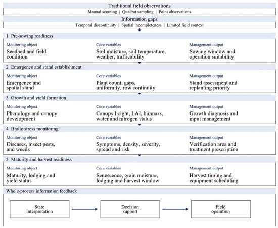
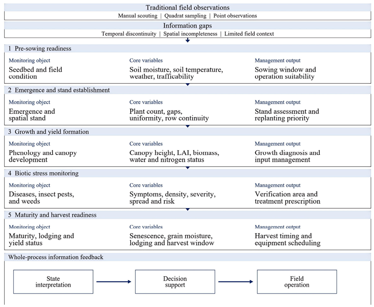
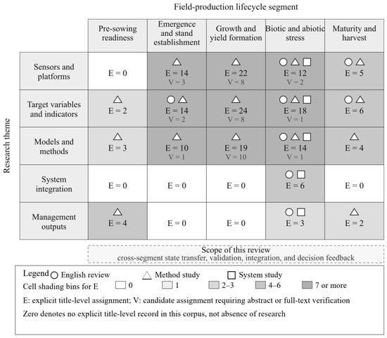
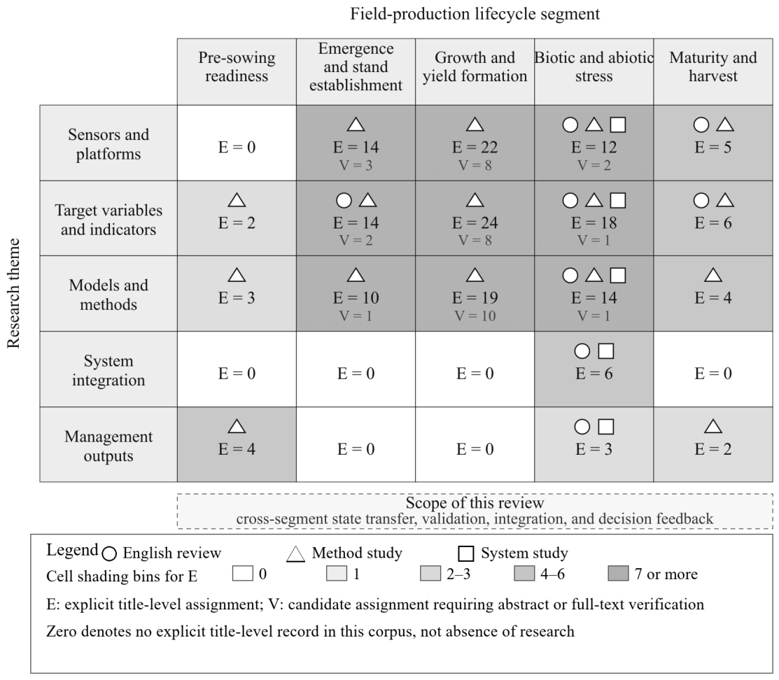
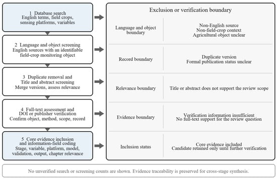
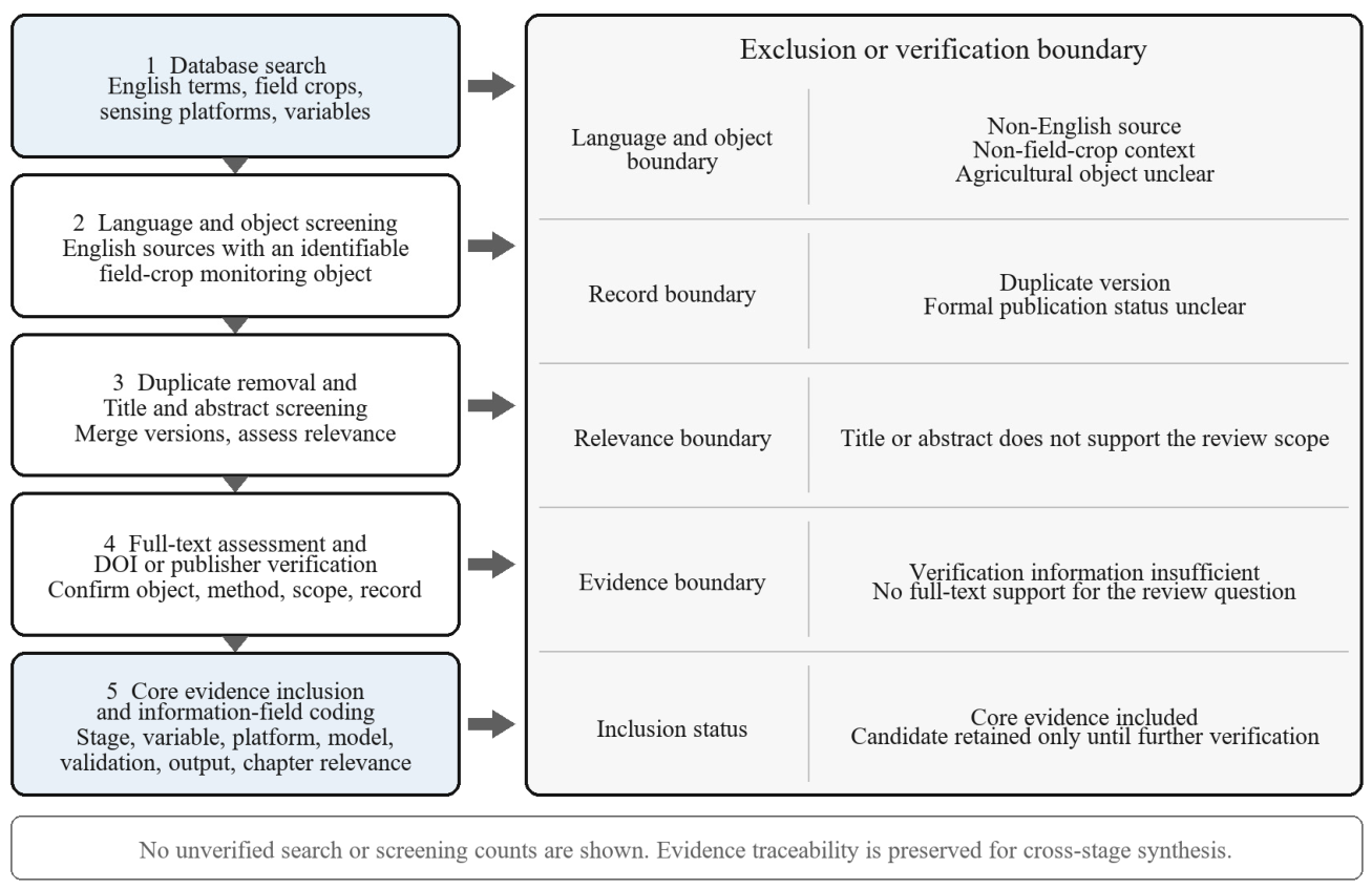
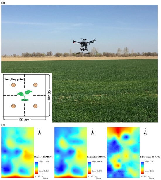
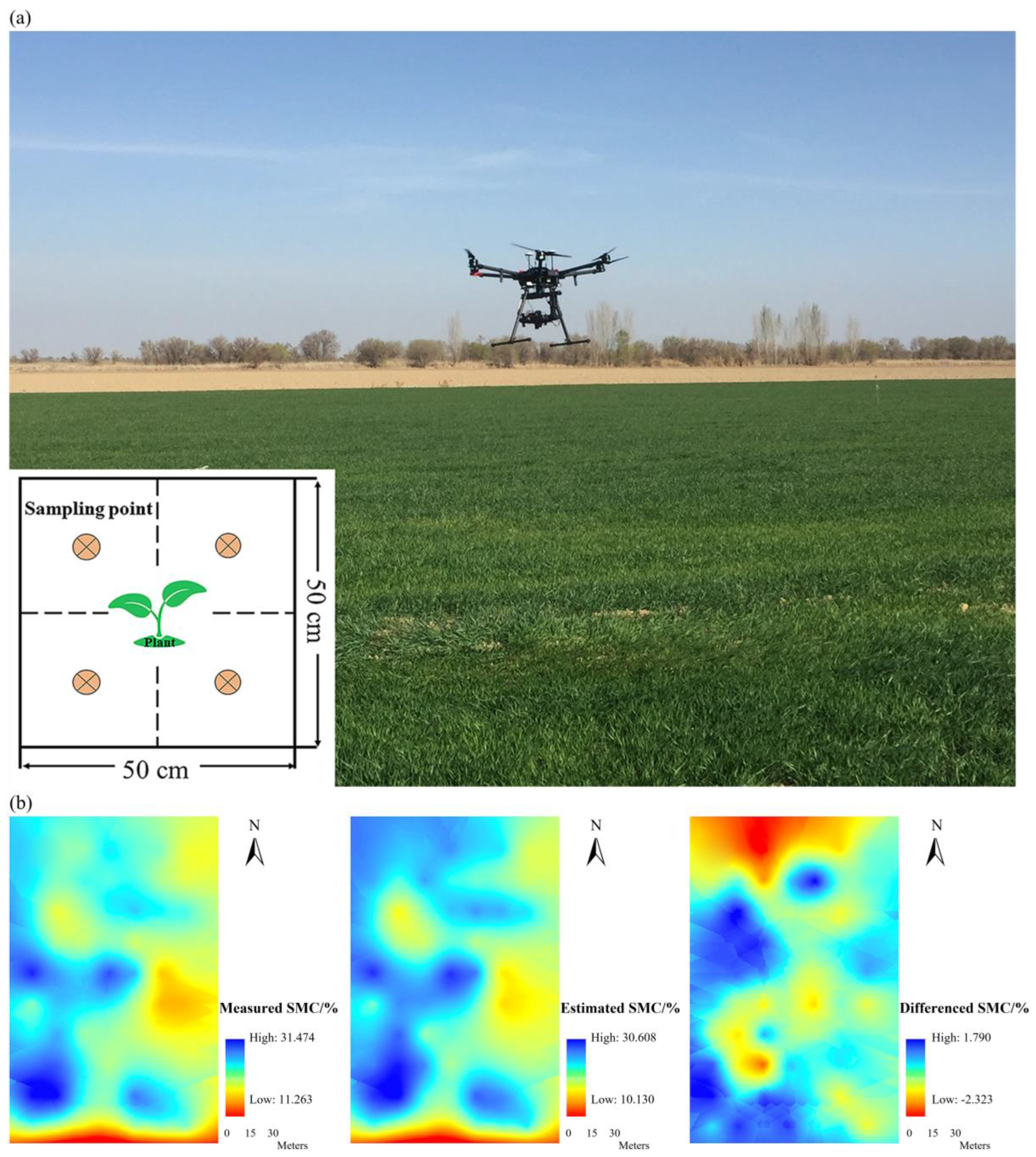
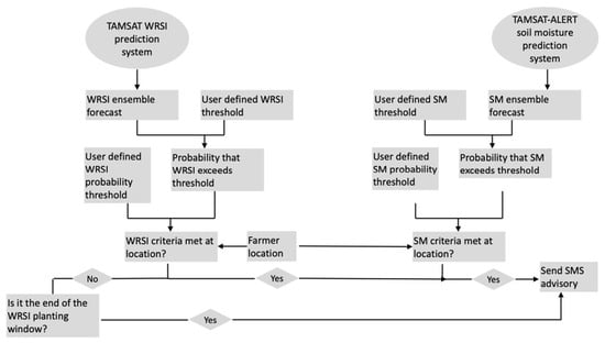
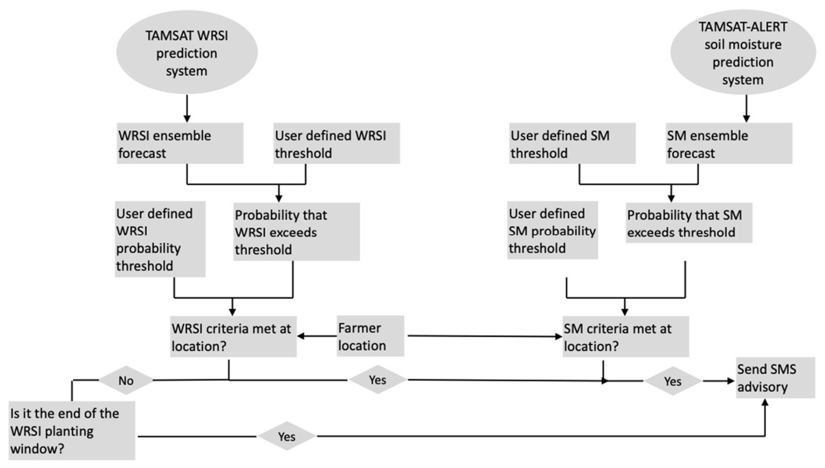
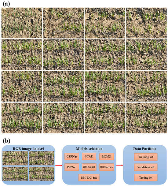
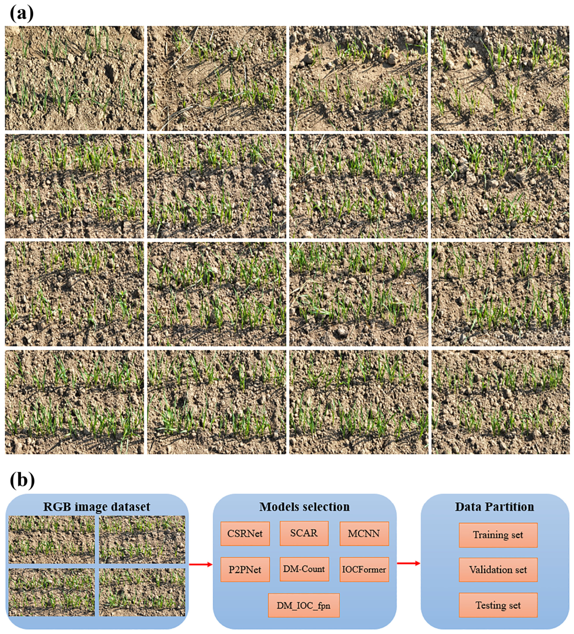
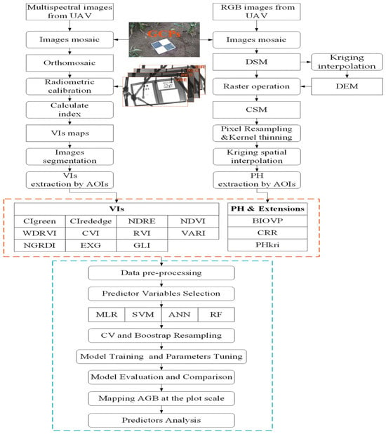
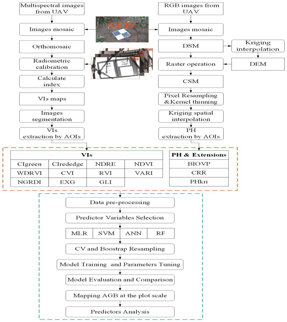
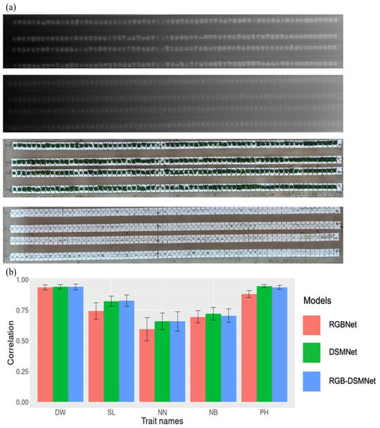
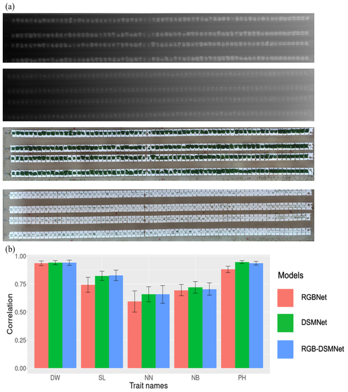
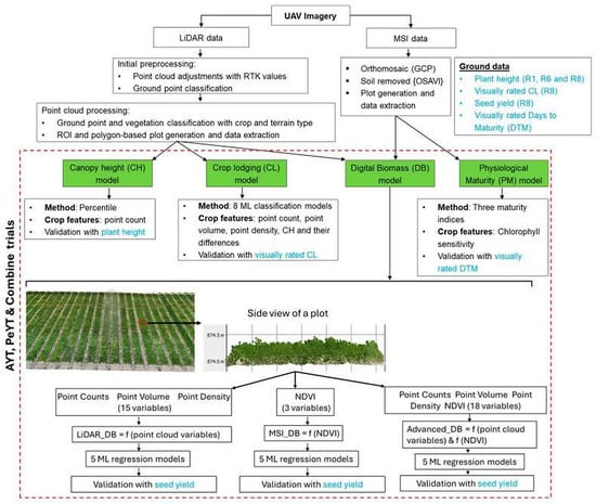
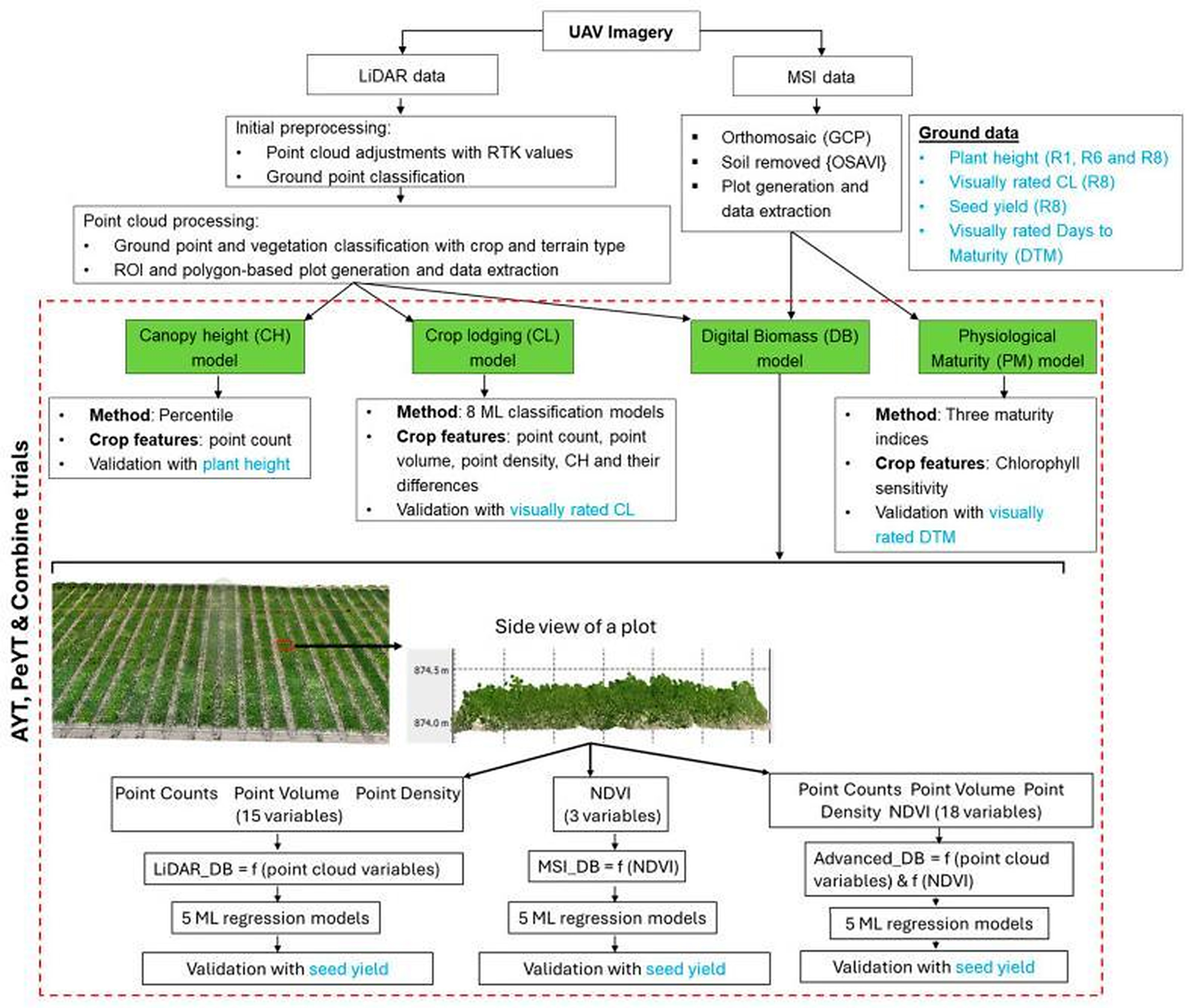
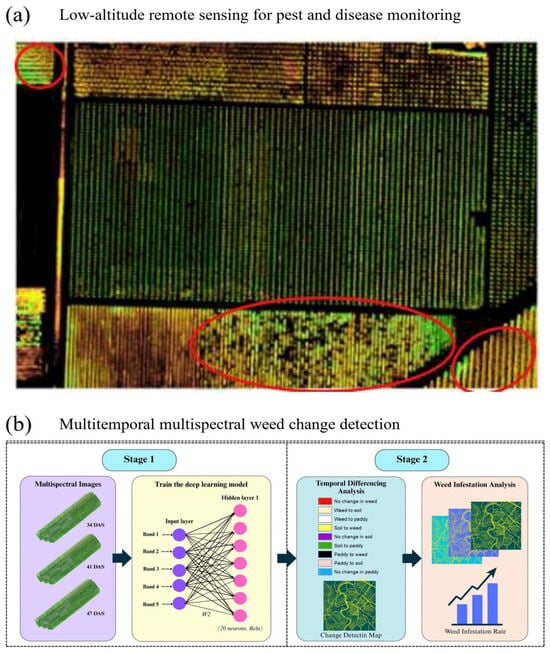
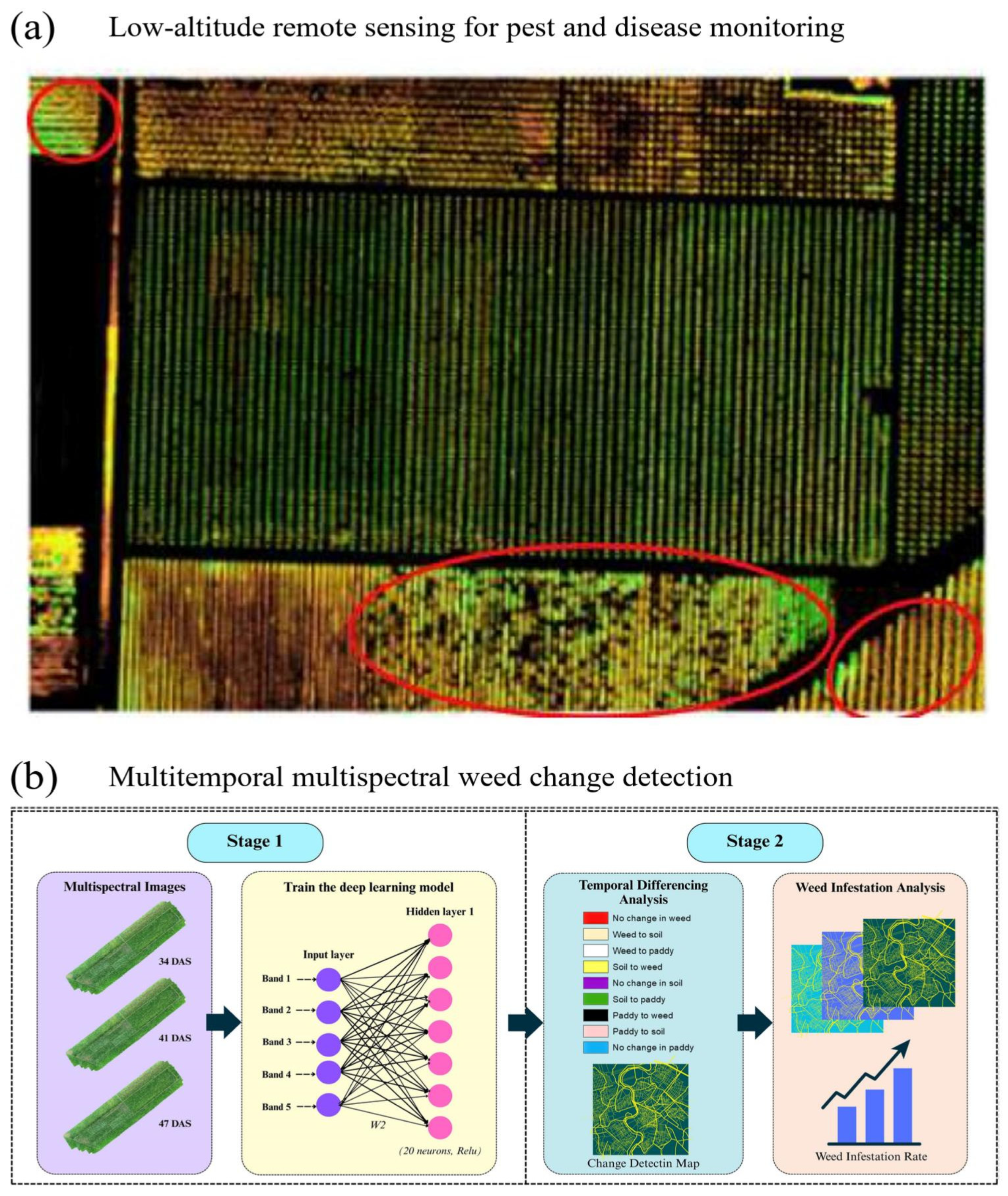
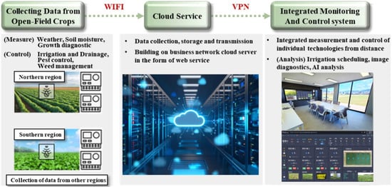
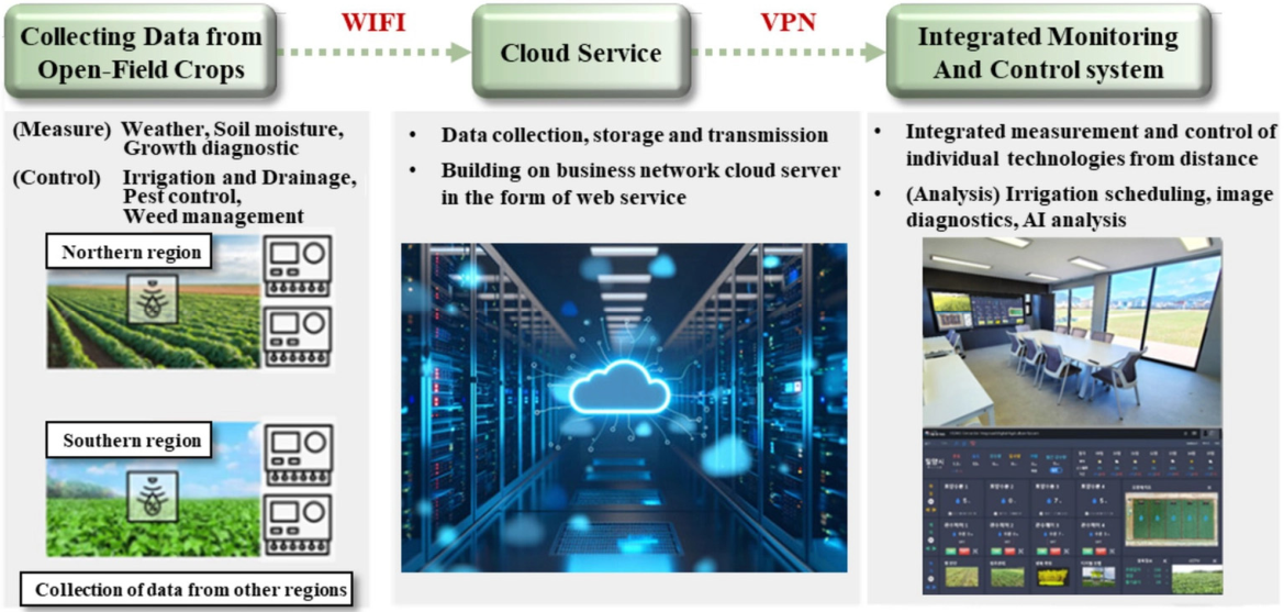
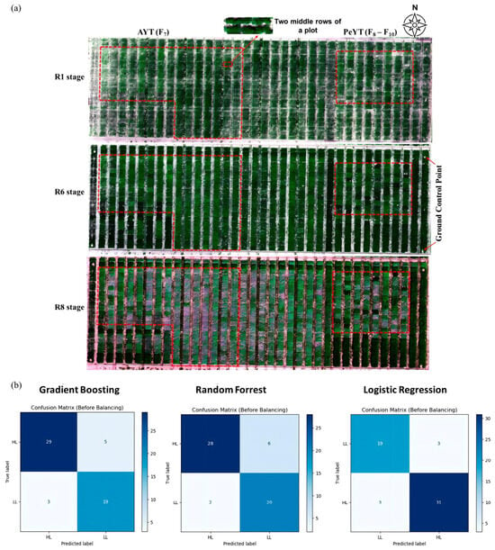
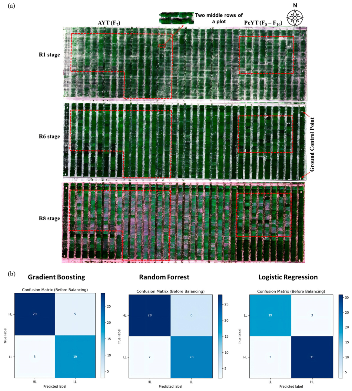
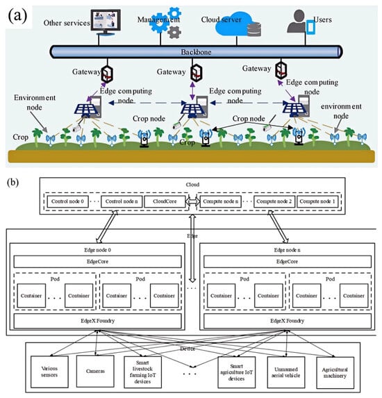
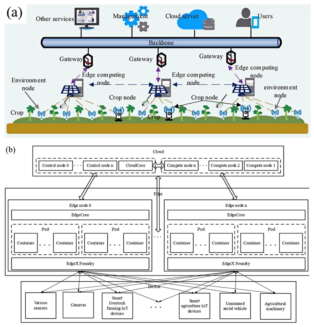
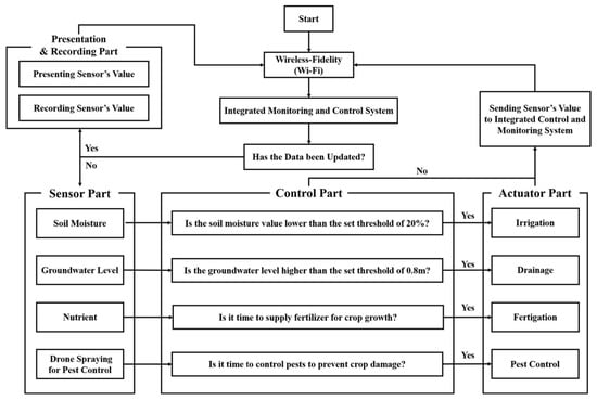
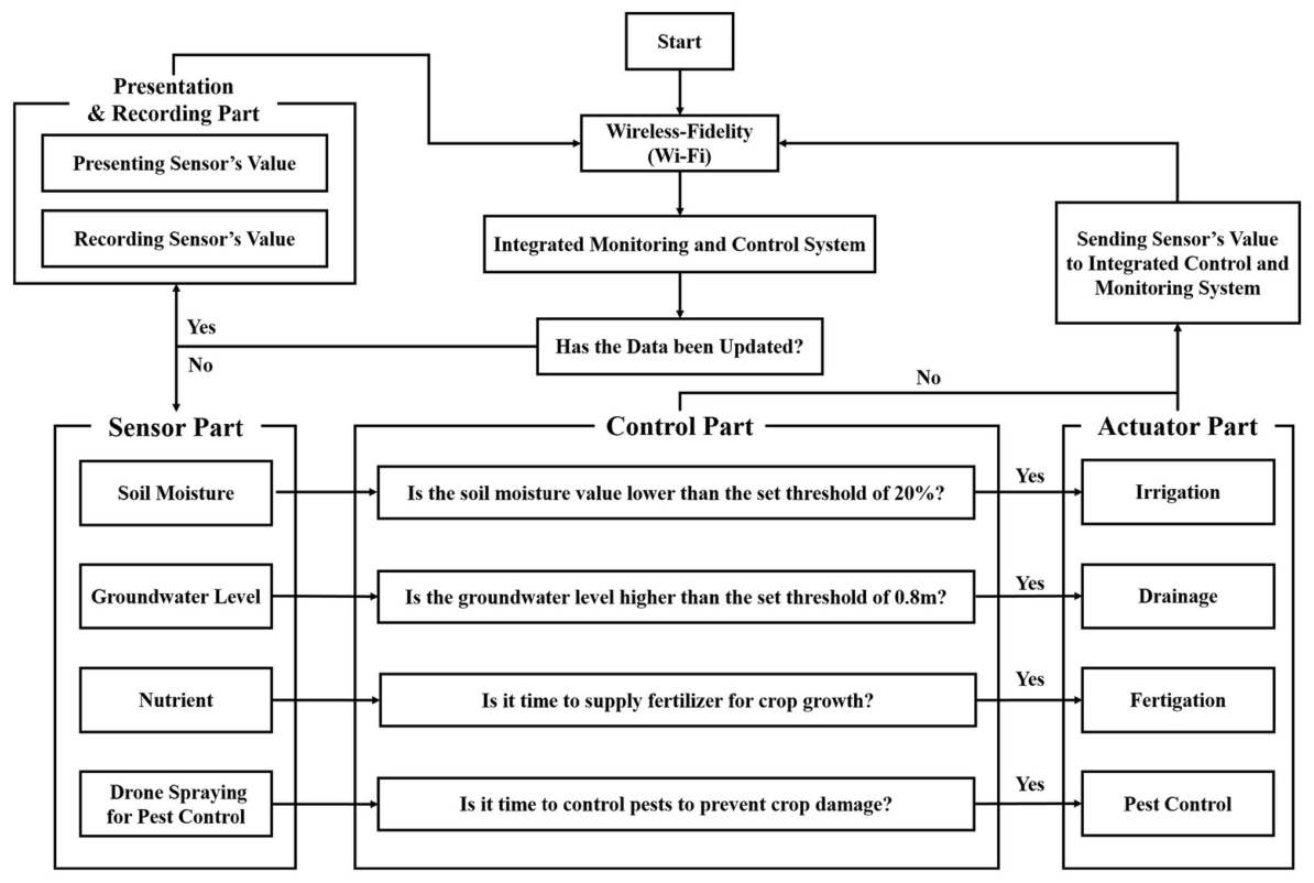
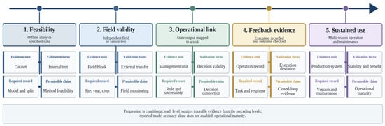
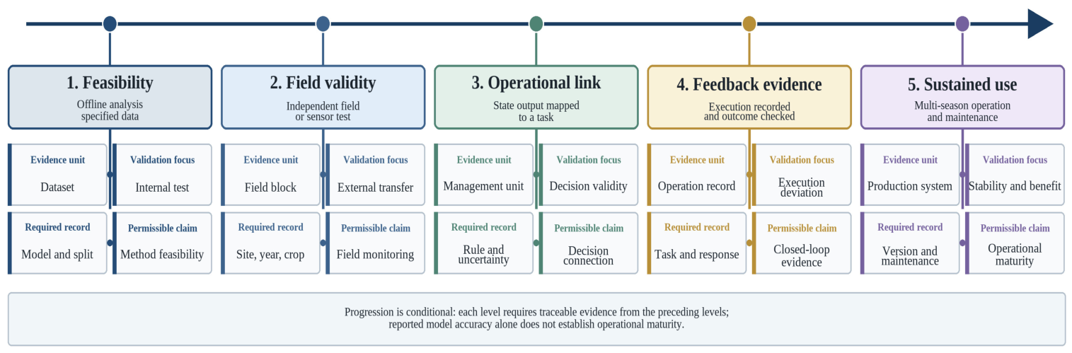
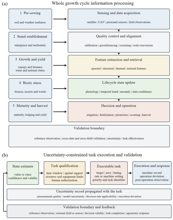
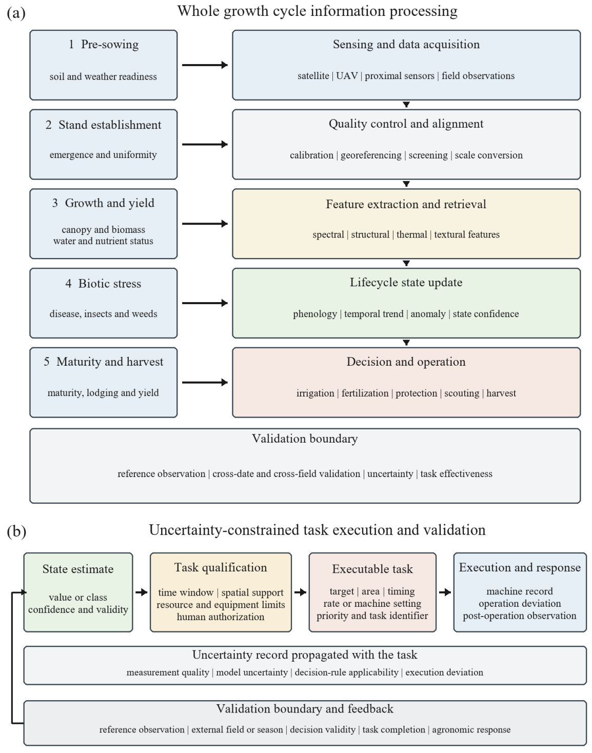

Disclaimer/Publisher’s Note: The statements, opinions and data contained in all publications are solely those of the individual author(s) and contributor(s) and not of MDPI and/or the editor(s). MDPI and/or the editor(s) disclaim responsibility for any injury to people or property resulting from any ideas, methods, instructions or products referred to in the content. |
© 2026 by the authors. Licensee MDPI, Basel, Switzerland. This article is an open access article distributed under the terms and conditions of the Creative Commons Attribution (CC BY) license.