


Abstract
The nematic mesogens within dielectric liquid crystal elastomers (DLCEs) rotate in response to external electric fields, thereby driving macroscopic active shape morphing. This work establishes a rigorous theoretical framework to investigate the electro-mechanical bending mechanics of cantilevered DLCE sheets governed by this actuation mechanism. By theoretically formulating the electromechanical effect as a localized spontaneous strain field, we analytically correlate the stress-free deformation with the local nematic director alignment. We demonstrate that the macroscopic bending morphology of the DLCE sheet can be deterministically programmed by tailoring the principal bending directions via this microscopic director design. Our findings reveal that the synergistic interplay between the tailored spontaneous curvature and cantilever boundary constraints generates a rich variety of three-dimensional configurations, enabling active regulation of both deflection and out-of-plane tilting at the free edge. Furthermore, we explicitly highlight the critical, yet often overlooked, role of spontaneous shear strain, which significantly governs the bending response even within the thin-plate limit. These theoretical insights establish a robust foundation for the structural design of DLCE-based directional soft actuators and flexible devices.
1. Introduction
As the most prevalent deformation mode in thin-walled structures, active bending from a two-dimensional (2D) flat sheet into a complex three-dimensional (3D) configuration under external stimuli can fulfill various engineering requirements. Representative applications include untethered locomotion [1], soft grasping [2], and the formation of dynamic surface morphologies [3].
Liquid crystal elastomers (LCEs) are fundamentally crosslinked polymer networks that inherently incorporate liquid crystal mesogens into their molecular architecture [4]. By coupling the orientational order of liquid crystals with the mechanical deformability of the polymer network, LCEs have emerged as a prominent class of smart soft materials. They are capable of undergoing active shape morphing in response to diverse environmental stimuli, such as thermal [5], photonic [6], electromagnetic [7,8], and moisture fields [9]. A hallmark of LCEs is their highly programmable active deformation [10,11]. By judiciously engineering the nematic director field during material fabrication to define the local average alignment of the integrated liquid crystal mesogens [12], a rich variety of macroscopic bending behaviors can be intricately encoded into the structure [1]. Consequently, LCE sheets have been extensively explored as soft bending actuators and sensors [1,13]. For example, photo-responsive LCE bending has been utilized to replicate the biological iris, allowing for adaptive pupil size adjustment based on ambient light intensity [14]. Additionally, thermally and optically driven bending is widely applied to construct complex 3D surface topographies [15] and facilitate diverse locomotive modes, ranging from crawling and creeping to walking and swimming [16].
While the majority of current research emphasizes heat- or light-driven actuation, investigations into the direct electro-actuation of LCE sheets remain relatively sparse. This is surprising given that dielectric liquid crystal elastomers (DLCEs) exhibit outstanding electromechanical properties, including substantial actuation strain, rapid response times, and high energy conversion efficiency [7,8,10,17]. The electro-induced deformation in DLCEs stems primarily from the reorientation of nematic directors, a phenomenon that is particularly pronounced in swollen samples [8]. We have previously conducted preliminary explorations into the bending mechanics associated with this mechanism [18,19,20,21]. For instance, it was demonstrated that electro-induced bending can be effectively programmed via non-uniform director distributions [20], and the shape-morphing from flat plates to surfaces with zero, negative, or positive Gaussian curvatures was further detailed [19]. However, these previous studies were strictly confined to unconstrained, free-standing DLCE sheets. Since boundary constraints are almost inevitable in practical soft robotic applications, the mechanics of constrained DLCE structures remain a critical missing piece. This research status makes the application of LCEs as electroactive materials lag behind some other electroactive materials, such as piezoelectric materials [22], ferroelectric polymers, and dielectric elastomers [23]. To advance this field, the present study systematically investigates the highly programmable bending behaviors of cantilevered DLCE sheets by manipulating their principal bending directions. Furthermore, recognizing that director reorientation intrinsically produces a considerable magnitude of spontaneous shear strain, we place a special emphasis on analyzing the profound impact of this shear effect and its synergistic coupling with the clamped boundary on the overall bending kinematics, including the distinct out-of-plane free-edge tilting.
The remainder of this article is structured as follows. Section 2 outlines the electro-induced deformation mechanism and the formulation of spontaneous strains in DLCEs. Subsequently, the bending response is theoretically modeled utilizing the Reissner-Mindlin (RM) plate theory, wherein the electrical actuation is mathematically represented by spontaneous curvatures and equivalent spontaneous shear strains. Section 3 illustrates how tuning the nematic director alignment allows for the active manipulation of principal bending directions, thereby generating a diverse array of programmable shapes for cantilevered DLCE sheets. The specific influence of the shear strain is also thoroughly discussed. Finally, concluding remarks are provided in Section 4.
2. Theory for the Electric-Field-Induced Bending of DLCE Sheets
2.1. Spontaneous Strains
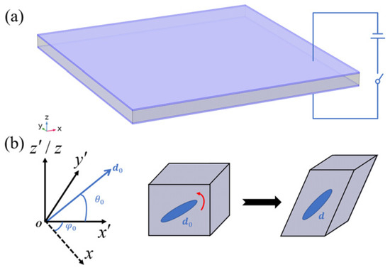
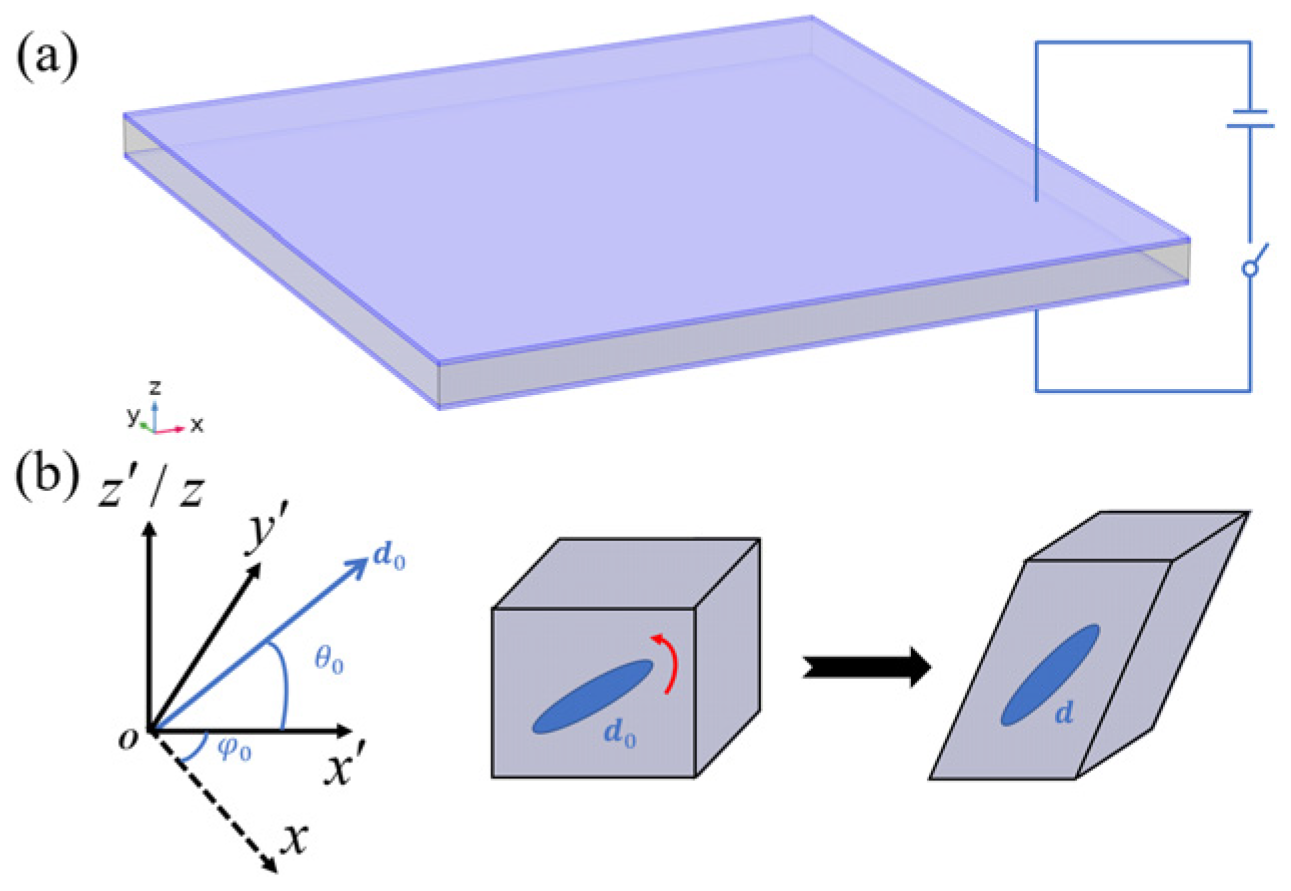
Consider a DLCE sheet of thickness h sandwiched between two perfectly compliant electrodes with negligible electrical resistance and mechanical stiffness as illustrated in Figure 1a. Upon application of a voltage V across the thickness, the sheet undergoes active deformation. This deformation fundamentally comprises a spontaneous term, which stems from the reorientation of the nematic director and is intrinsically stress-free. The spontaneous strain tensor can be expressed as [20].
Figure 1.
(a) Schematic of the dielectric liquid crystal elastomer sheet; (b) spontaneous deformation due to nematic director reorientation.
The initial director field can be synthetically programmed during material fabrication via various alignment techniques [12], whereas the current director is dynamically driven by the applied electric field [20]. For a DLCE sheet endowed with a through-thickness director gradient, i.e., , the structure behaves analogously to a functionally graded material. Upon electrical actuation, the induced electric field, the updated director orientation, and the resulting spontaneous strain all exhibit spatial gradients along the thickness direction [20]. Consequently, the sheet inherently undergoes a macroscopic bending deformation. Since even an infinitesimal strain can induce pronounced bending curvatures in thin-walled structures, we formulate the electromechanical bending model based on the small-strain assumption, corresponding to an actuation regime with a relatively low electric field intensity. To rigorously underpin this macroscopic formulation, the general 3D electromechanical governing equations are derived via the principle of virtual work in Appendix A.
By systematically formulating an asymptotic reduction under a relatively weak electric field (detailed in Appendix B), the spontaneous strain (1) can be analytically approximated as [18,19,20]
where the tensor describes the local plane spontaneous strain in the plane spanned by the local director and the z-axis (i.e., the coordinate system depicted in Figure 1b):
Here, is the out-of-plane tilt angle between the initial director and the x-y plane, and is a phenomenological material parameter reflecting the elastic constraint imposed by the polymer network on the mesogens. As derived in Appendix C, the local electric field intensity along the thickness direction E is given by
where is the nominal electric field intensity, while and denote the local the normal dielectric coefficient along the thickness and its through-thickness equivalent mean, respectively:
Here, and are the dielectric constants along and perpendicular to the director, respectively. For positive dielectric DLCEs (i.e., ) incorporating rod-like mesogens (i.e., ), the directors tend to reorient toward the vertical electric field within the local plane. This electro-rotation actively increases the out-of-plane tilt angle, thereby shortening the in-plane projection of the director as illustrated in Figure 1b. Consequently, a contractile local normal spontaneous strain is generated (i.e., ). Furthermore, director reorientation inevitably alters the oblique projection within the local plane, thereby inducing a coupled local spontaneous shear strain . The tensor in Equation (2) serves as the local coordinate transformation matrix between the and coordinate systems,
where is the azimuthal angle between the and planes. It is worth noting that when , reduces to the identity tensor, simplifying the spontaneous strain to . By integrating Equations (2)–(6), the electric-field-induced spontaneous strain is analytically formulated as an explicit function of the applied voltage V and the initial director alignment angles ( and ). This mathematical directness confirms that the macroscopic spontaneous strain field is highly programmable and can be deterministically encoded via microscopic director patterning. It is worth emphasizing that for a DLCE sheet with a through-thickness director gradient, where and , the spontaneous strain becomes a highly localized field variable, i.e., .
Moreover, according to Equation (3), the spontaneous shear strain and normal strain share the same order of magnitude. Such a significant shear strain effect can profoundly influence the global bending deflection and curvature of the sheet, particularly under clamped boundary conditions [20,24,25,26]. Therefore, to accurately capture these shear-dominated kinematics, the classical RM plate theory is employed in the subsequent sections to model the bending behavior of the constrained DLCE sheets.
2.2. Governing Equations of Spontaneous Bending Under Reissner-Mindlin Kinematics
The displacement field of the DLCE sheet is mathematically formulated under the RM kinematics as
where denotes the transverse deflection of the mid-plane of the sheet, while and represent the rotations of cross sections about the y and x axes, respectively. Then, the total Cauchy strain components are expressed as
where the engineering shear strains are adopted.
Based on the variational formulation for the RM plate kinematics, the equilibrium equations are derived as
in which external transverse mechanical loads are omitted. The moment and transverse shear force per unit length are defined through thickness integration as
where represents the shear correction factor. The free and clamped boundary conditions, which constitute the primary configurations investigated in this study, are expressed as
and
respectively, where the subscripts n and s denote the directions normal and tangential to the boundaries, while represent the direction cosines of the outer normal on the boundary.
Since the total deformation of the active DLCE incorporates an intrinsic spontaneous component, the elastic strain is formulated under the small-strain assumption as the difference between the total strain and the spontaneous strain, yielding
Combining Equations (2), (3) and (6), the explicit components of the spontaneous strain field are analytically expressed as
where the corresponding spontaneous engineering shear strains are used, and the electric field intensity E is evaluated by Equation (4). The quantitative accuracy of these analytical approximations for both the localized electric field and the resulting non-linear spontaneous strains is rigorously evaluated against the 3D multi-field coupled finite element results in Appendix D. For the thin DLCE structure, the plane-stress assumption is physically reasonable. According to the linear Hooke’s law, the stress is expressed as
where is the elastic matrix of the DLCE sheet and assumed to be isotropic in this paper. and denote Young’s modulus and Poisson’s ratio, respectively. The shear modulus .
Then, substituting Equation (15) into Equation (10), the moment and transverse shear force read
respectively, where is the flexural rigidity, while the parameters and are determined by the spontaneous strain field and defined as
Specifically, evaluate the first moment of the in-plane spontaneous components across the thickness, and are thus identified as the spontaneous curvatures, while represent the through-thickness average of the spontaneous transverse shear strains, and are therefore termed the equivalent spontaneous transverse shear strains.
As introduced in the above section, for a DLCE sheet featuring an initial through-thickness director orientation gradient, the spontaneous strain components (14) vary strictly as functions of the thickness coordinate. Consequently, the resulting spontaneous curvatures and equivalent spontaneous transverse shear strains remain uniform constants that are entirely independent of the in-plane coordinates. Then, substituting Equation (16) into the equilibrium Equation (9), one can obtain the following dimensionless governing equations:
where the dimensionless quantities are defined as
and denotes the dimensionless Laplace operator. Compared with the classical RM plate model, the equivalent spontaneous shear strains (17) are uniquely introduced into the governing equations to represent the electric-field-induced strain effect within the plate kinematics. Furthermore, this effect also manifests in the boundary conditions. Specifically, by Equation (11), the dimensionless free boundary condition is formulated as
where and denote the normalized normal and tangential coordinates, respectively. The corresponding dimensionless spontaneous curvatures are given by
and
where . and are given by Equation (5). The equivalent spontaneous transverse shear strain on the boundary is
where
It should be noted that Equations (4), (14) and (17) have been substituted into Equations (22) and (24). Similarly, by Equation (12), the dimensionless clamped boundary condition is formulated as
Having fully derived the governing equations and corresponding boundary conditions, i.e., Equations (18)–(25), we proceed to solve these boundary-value problem numerically using finite element method (FEM) implemented in the COMSOL Multiphysics 6.2 software.
2.3. Finite Element Simulation and Spontaneous Curvatures
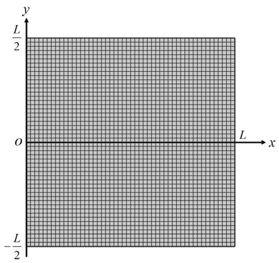
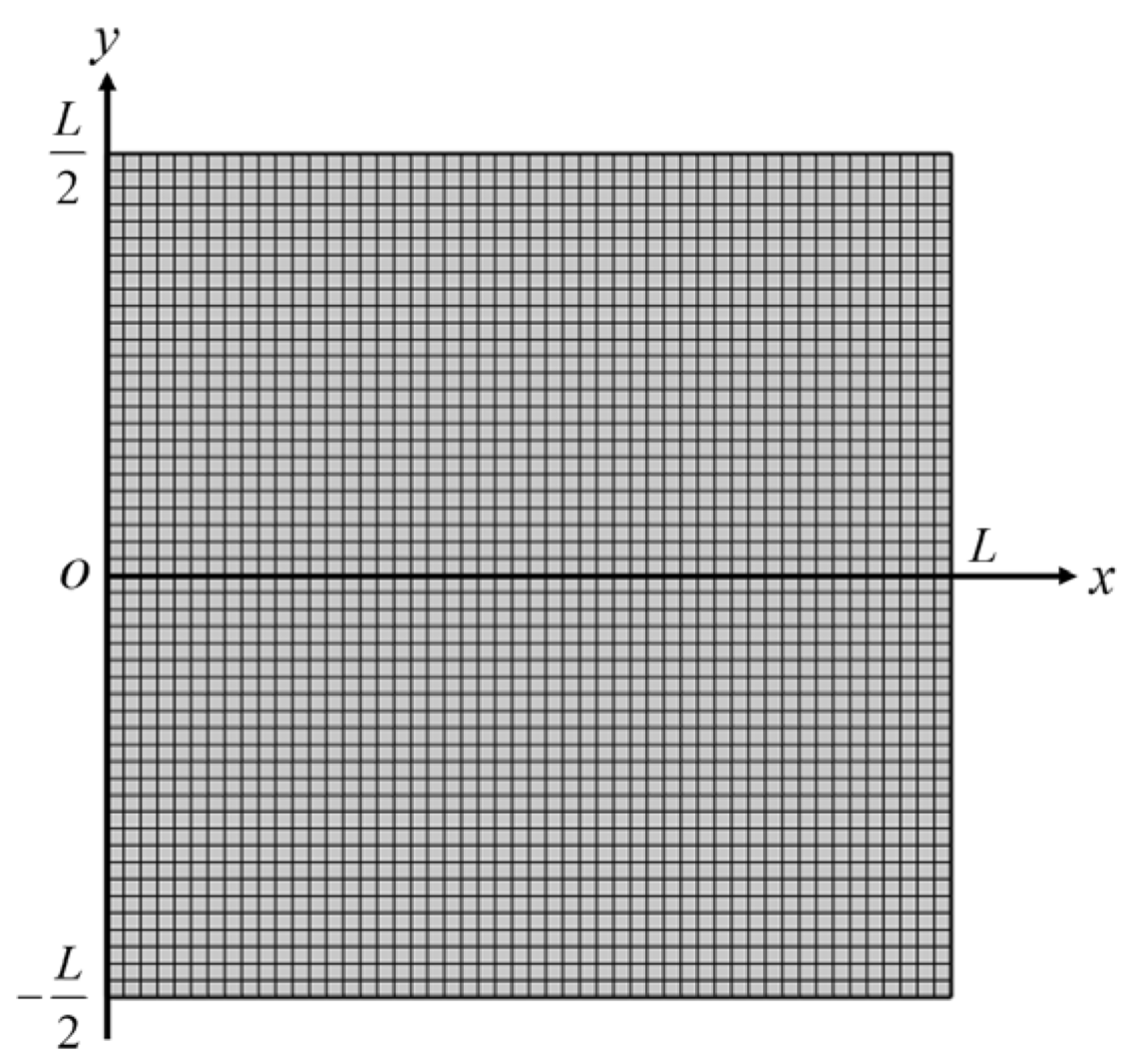
For the numerical simulations, a square DLCE sheet featuring a slenderness ration of is established as the representative computational model, as illustrated in Figure 2.
Figure 2.
Square sheet with square meshes. The slenderness ratio .
The boundary-value problem formulated by Equations (18)–(25), is implemented via the Plate Interface of the Structural Mechanics Module in the software. From a continuum mechanics perspective, the electric-field-induced spontaneous strain essentially acts as a stress-free eigenstrain. Therefore, to rigorously incorporate this physical mechanism into the numerical framework, the analytical spontaneous curvatures (22) and equivalent spontaneous transverse shear strains (24) are directly mapped onto the Initial Bending Strain and the Initial Transverse Shear Strain in the software as
This mapping procedure effectively introduces the electric-field-induced spontaneous strain effect into the numerical model. For a plate with a given initial geometry and boundary constraints, once the specific values of the components in Equation (26) are prescribed, the corresponding bending deformation can be uniquely determined. As revealed by Equations (22) and (24), the magnitudes of and are proportionally scaled by the square of the applied nominal electric field intensity . However, does not alter the relative proportions among the individual spontaneous curvature and equivalent spontaneous transverse shear strain components, and consequently has no influence on the specific bending morphology. The relative proportional relationships and the final spatial shape are exclusively dictated by the through-thickness distribution of the initial director orientations, i.e., and .
Since the present work primarily investigates the shape morphing encoded by the initial director alignment, we set the applied nominal electric field intensity to for all ensuing examples. This normalization strategy simplifies the theoretical expressions by successfully eliminating redundant material parameters. Following the literature [7], the material parameters adopted in the calculations are defined as: , , , and , where is the vacuum permittivity. To ensure numerical accuracy and convergence, the geometric domain is uniformly discretized by a square mesh as shown in Figure 2.
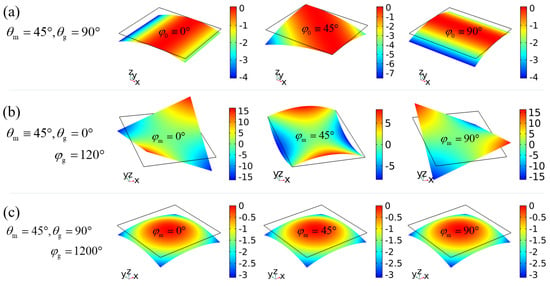
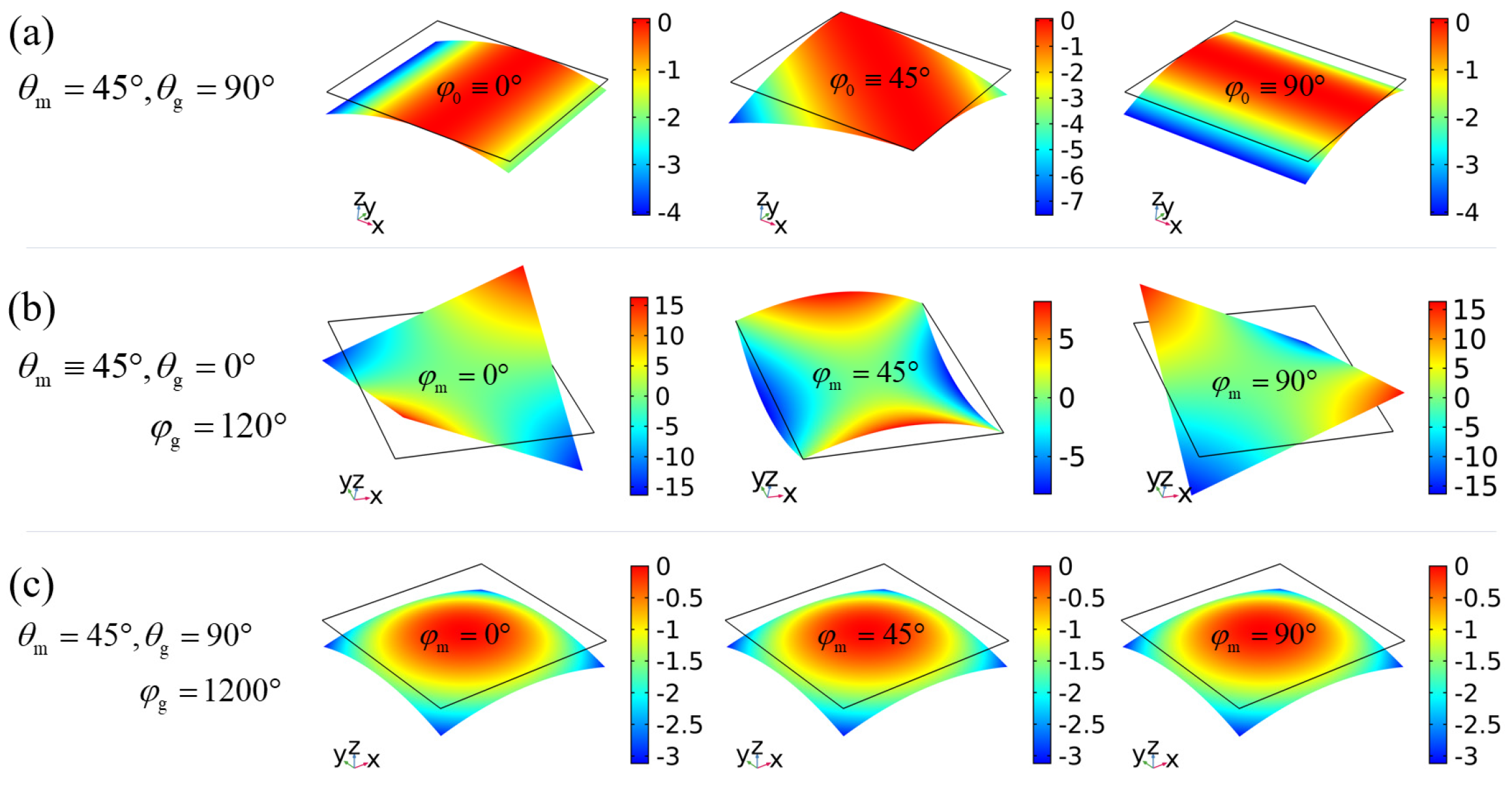
To systematically analyze the intrinsic spontaneous curvatures, we first investigate the benchmark case of free-standing DLCE sheets under unconstrained boundary conditions. The capability of the dimensionally reduced plate equations to capture these bending morphologies is thoroughly validated against the full 3D multi-field deformations detailed in Appendix D. As shown in Figure 3, flat sheets encoded with different initial director alignments can smoothly morph into distinct surfaces featuring zero (Figure 3a), negative (Figure 3b), or positive (Figure 3c) Gaussian curvatures. Analytically, by substituting the free boundary conditions (20) into the governing Equation (18), the bending curvature tensor of a free-standing sheet is found to identically equal its spontaneous curvature tensor (i.e., the Initial Bending Strain defined in Equation (26)):
Figure 3.
Electric-field-induced bending of free-standing sheets. (a) Unidirectional bending with zero Gaussian curvature encoded by splay-bend (SB) director orientation alignments. (b) Bending with negative Gaussian curvature encoded by TB alignments. (c) Bending with positive Gaussian curvature encoded by STB alignments.
This exact analytical correspondence, which aligns with the solutions derived from the classical Kirchhoff–Love (KL) plate theory in our previous work [19], serves as a direct baseline to verify our numerical simulations. Given the small thickness of the sheet, the through-thickness director profile is reasonably considered to be linearly distributed:
where and denote the director orientations at the middle plane (), while and represent their respective spatial gradients through the thickness. Once the dielectric constants are specified, the individual components of the spontaneous curvature tensor (27) become explicit functions of the four design parameters (,,,), allowing for deterministic control over the morphing modes. Based on the gradient parameters and in Equation (28), the typical through-thickness director alignments utilized for shape programming can be logically classified into three fundamental configurations. Specifically, the splay-bend (SB) alignment is characterized by a pure out-of-plane tilt gradient (i.e., and ), the twist-bend (TB) alignment features a pure azimuthal twist gradient (i.e., and ), and the more complex splay-twist-bend (STB) alignment combines both gradients (i.e., and ). From an experimental perspective, realizing these deterministic alignments is highly feasible. The SB alignment can be readily produced using hybrid surface-anchoring templates [27], while the TB and STB alignments can be successfully fabricated via advanced photo-alignment techniques [11,12] or multi-layer 3D printing technologies [9].
For the case where the director is aligned as the SB type, i.e., and , the sheet generally bends in only one direction like a beam as shown in Figure 3a, because the internal spontaneous strain reduces to a plane strain state as given in Equation (3). The spontaneous curvature tensor (27) in this scenario specializes to
where the scalar curvature intensity depends only on the SB alignment through the following integral:
From Equation (29), the two spontaneous principal curvatures and Gaussian curvature are analytically derived as
Meanwhile, the corresponding principal directions form angles of
with respect to the x-axis. As clarified by Equations (31) and (32), it is obvious that the bending magnitude of SB sheets is explicitly regulated by the out-of-plane SB parameters , whereas the direction of the bending axis is strictly controlled by the azimuthal angle .
In contrast, for the case of the TB configuration characterized by and , the sheet generally bends into a saddle surface possessing a negative Gaussian curvature as shown in Figure 3b. In this scenario, the spontaneous curvature tensor (27) specializes to
where is given by
Accordingly, the spontaneous principal curvatures and the resulting negative Gaussian curvature are obtained as
And the corresponding principal directions form angles of
with respect to the x-axis, respectively. It follows from (34)–(36) that the mean curvature of the saddle surface vanishes identically, i.e., . Furthermore, the bending magnitude is modulated by the out-of-plane angle and the through-thickness azimuthal gradient , whereas the spatial orientation of the saddle is determined by the mid-plane azimuthal angle .
Beyond bending configurations yielding zero or negative Gaussian curvatures, positive Gaussian curvatures can be achieved via the general STB director alignment where and simultaneously, as shown in Figure 3c. A more comprehensive analytical treatment of these free-standing morphing modes is detailed in our previous work [19].
The consistent agreement between the analytical baselines and numerical results verifies the predictive capability of the implemented plate model. The above results show that the free-standing DLCE sheet can present abundant programmable bending shapes under the domination of the spontaneous curvature. We will next study the bending behavior of cantilevered DLCE sheets, in which the boundary constraints make the bending shapes more complex but more interesting. And the effects of spontaneous shear strain on bending additionally emerge.
3. Bending Behaviors of Cantilevered DLCE Sheets
3.1. Deflection of Cantilever Sheets Caused by Spontaneous Shear Strains
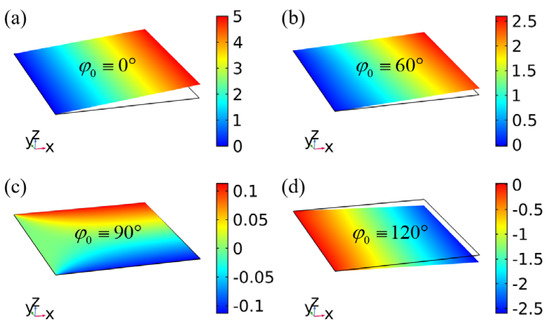
We consider the cantilever sheet whose left edge () is clamped. When the director is uniformly distributed throughout the sheet, i.e., , , and , the spontaneous strain (14) is perfectly uniform, meaning the free-standing sheet would not undergo any bending deformation. However, as dictated by Equations (5), (22), (24) and (28), although this uniform director alignment leads to vanishing spontaneous curvatures, i.e., , the equivalent spontaneous shear strains remain non-zero. Consequently, a noticeable deflection (and even a slight bending curvature) is induced in the cantilever sheet as shown Figure 4.
Figure 4.
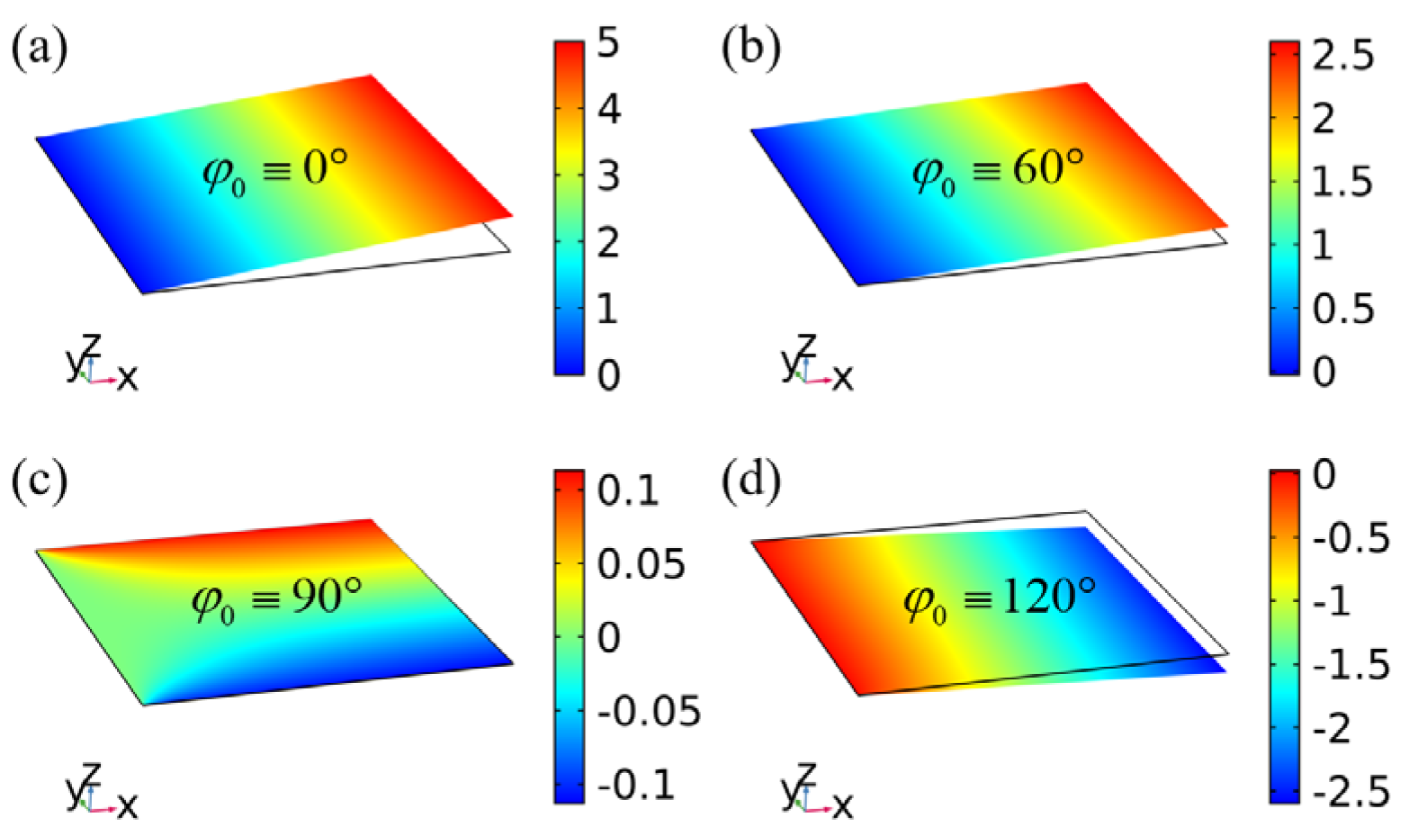
Bending of cantilever sheets with uniform director orientations. The orientation is . (a) Deformation contour with ; (b) Deformation contour with ; (c) Deformation contour with ; (d) Deformation contour with . The color bar represents the dimensionless transverse deflection .
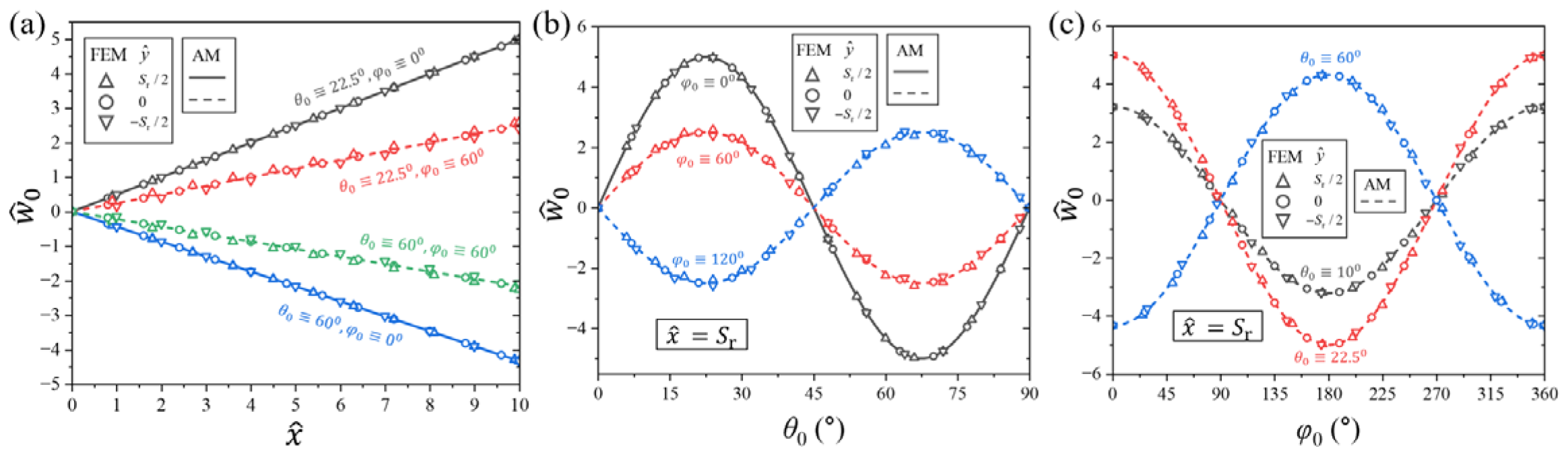
For a sheet where the directors are aligned and rotated uniformly within planes parallel to the x-z plane, i.e., the orientations , a homogeneous spontaneous plane strain state (3) is generated within the x-z plane. Because the x-z plane is perpendicular to the clamped edge of the sheet and the cross section at the clamped boundary cannot rotate, the spontaneous shear strain forces the sheet to undergo a rigid-body rotation around the clamped edge as shown in Figure 4a. In this case, the deflection is a linear function of and can be accurately fitted by (see the solid lines in Figure 5a,b).
where the spontaneous shear strain (14) reads
by using Equations (4) and (5), and . Mechanically, the periodicity and symmetry of the spontaneous shear strain with respect to the orientation and are due to the nematic symmetry of material and objective geometric symmetry. Specifically, reaches its extreme values at orientations and vanishes identically at .
Figure 5.
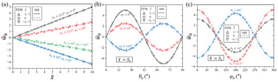
Deflection of cantilever sheets with uniform director orientations. The solution obtained by analytical method (AM) is given by Equations (37)–(39). (a) Curves of deflection along the plate length under different orientation parameters; (b) Variation curves of deflection with tilt angle at ; (c) Variation curves of deflection with azimuthal angle at .
For sheets featuring other orientations, the directors are no longer aligned and rotated within planes perpendicular to the clamped edge. Thus, the deflection is no longer a simple single-variable function of like Equation (37) as shown in Figure 4b–d. However, because the variation of along the direction is small enough to be neglected (see Figure 5), Equation (37) can still be safely adopted to evaluate the primary deflection profile, where the spontaneous shear strain component (14) is expressed as
This expression successfully generalizes Equation (38) and remains applicable to any arbitrary . As a function of , reaches its peak magnitudes at and , which corresponds to the case analyzed above. Conversely, at and , where the directors are aligned within planes parallel to the clamped boundary and perpendicular to the x-z plan.
According to the linear deflection function (37), the bending curvature of the cantilever sheet remains zero. This confirms that the deflection is entirely driven by the rigid-body rotation induced by the homogeneous spontaneous shear strain. If a non-uniform spontaneous curvature is encoded into the cantilever sheet via SB or TB director alignments, true bending curvatures will be activated, thereby giving rise to much more diverse and interesting morphing shapes, as discussed below.
3.2. Multi-Directional Bending and Free Side Tilting of Cantilever Sheets by Rotating the Principal Direction of Spontaneous Curvature
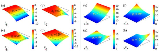
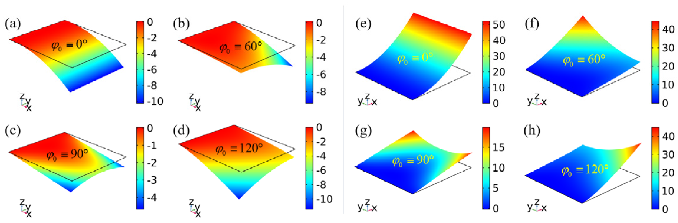
We first consider the cantilever sheet featuring a single non-zero spontaneous principal curvature but a vanishing spontaneous Gaussian curvature, encoded by the SB director alignment. As shown in Figure 6, due to the addition of the spontaneous curvature effect, the resulting bending deflection is generally larger than pure-shear case analyzed in Section 3.1.
Figure 6.
Bending of cantilever sheets with SB director orientation alignments. (a–d) correspond to the SB.MC alignment . (e–h) correspond to the SB.MAX alignment .
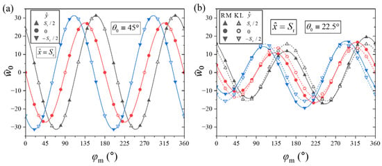
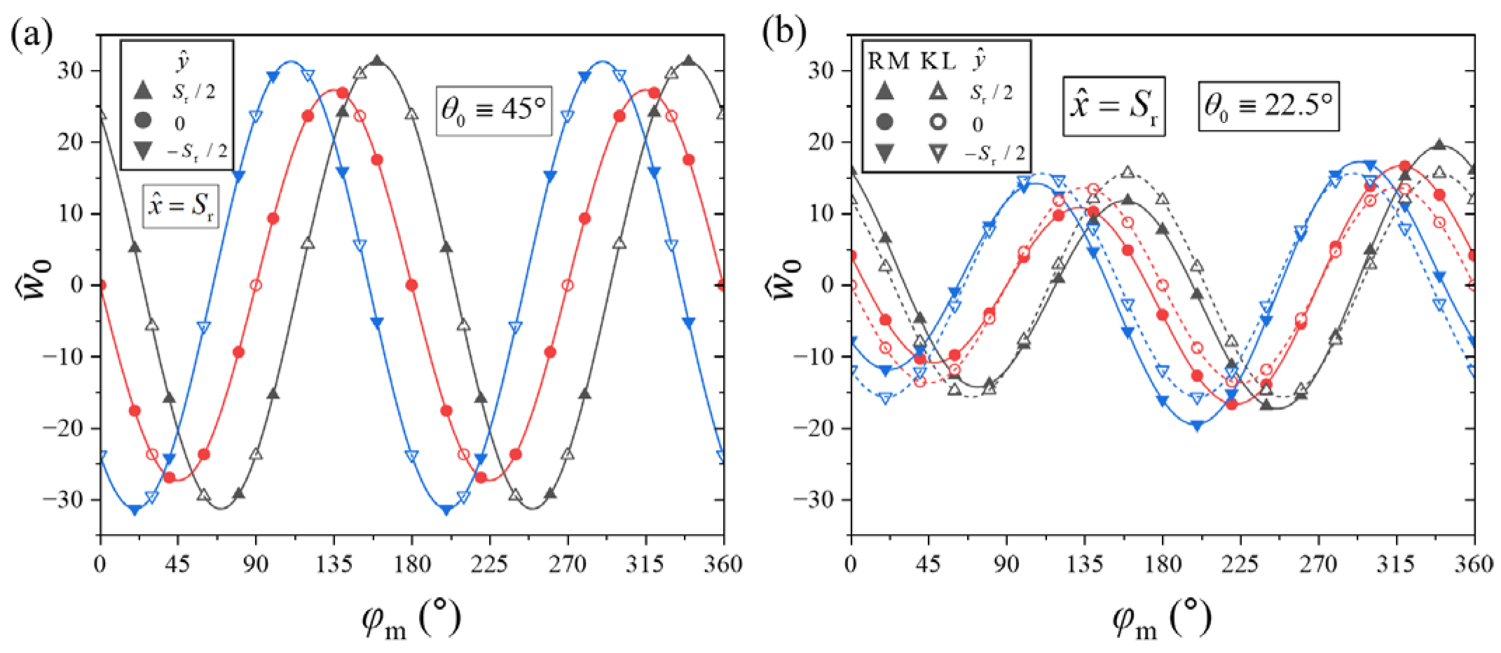
For a sheet where the clamped edge is exactly perpendicular to the preferred free-bending direction (e.g., at an orientation ), the structure exhibits simple unidirectional bending like a beam, meaning , as shown in Figure 6a,e and the black lines in Figure 7a,c. Under this unidirectional bending assumption, i.e., , , and , the governing Equation (18) reduces to
Figure 7.
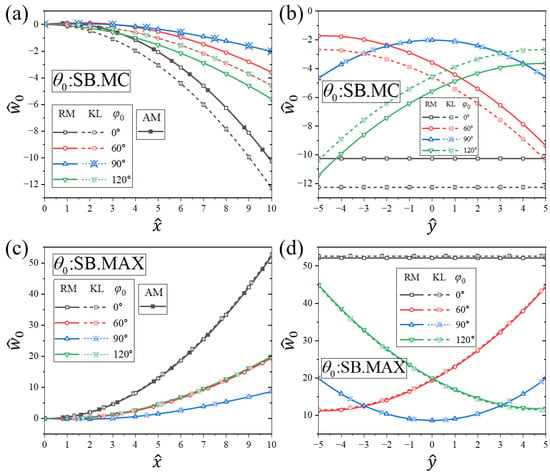
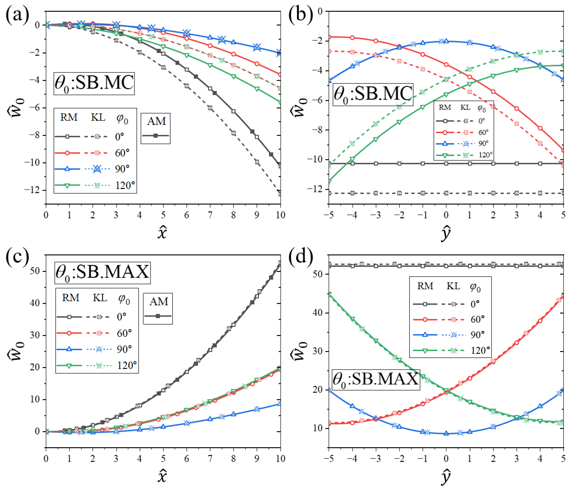
Deflection of cantilever SB sheets. The solid and dashed lines are plotted by FEM based on RM and KL plate theories, respectively. The solution obtained by AM in the condition of is given by Equation (44). (a) Longitudinal deflection along for SB.MC alignment ; (b) Transverse deflection along for SB.MC alignment ; (c) Longitudinal deflection along for SB.MAX alignment ; (d) Transverse deflection along for SB.MAX alignment .
The general solutions to these ordinary differential equations are derived as
and
where the four integration constants, , , , and , are uniquely determined by the boundary conditions. The clamped conditions (25) at and free boundary conditions at are defined as
Then, combining Equations (41)–(43), the deflection of unidirectional bending of the cantilever sheet can be obtained as
where (30), and (24) reads
Equation (44) explicitly shows that the bending curvature depends entirely on the spontaneous curvature . The SB alignment (denoted as SB.MC) represents the most common configuration utilized in experiments and practical applications [14,27]. Since the resulting value is negative, the SB.MC sheet bends downward, as illustrated by Figure 6a and the black lines in Figure 7a. However, in our parameter () setting, does not represent the global maximum of the function . Instead, the maximum curvature magnitude (exceeding that of the SB.MC case by more than four times) is achieved near (denoted as SB.MAX). Because is positive, the SB.MAX sheet bends upward with a tighter curvature, as confirmed by Figure 6e and the black lines in Figure 7c. Crucially, Equation (44) indicates that the spontaneous transverse shear strain has no direct impact on the bending curvature itself, but instead induces a pure rigid-body rotation that scales the overall deflection.
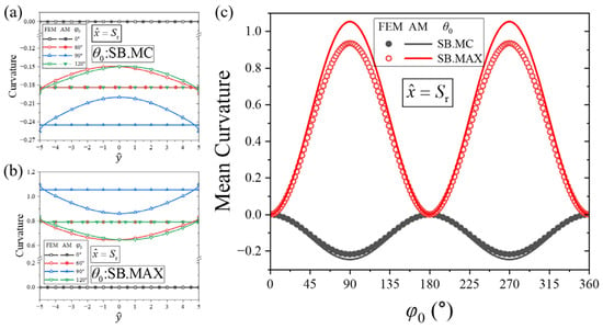
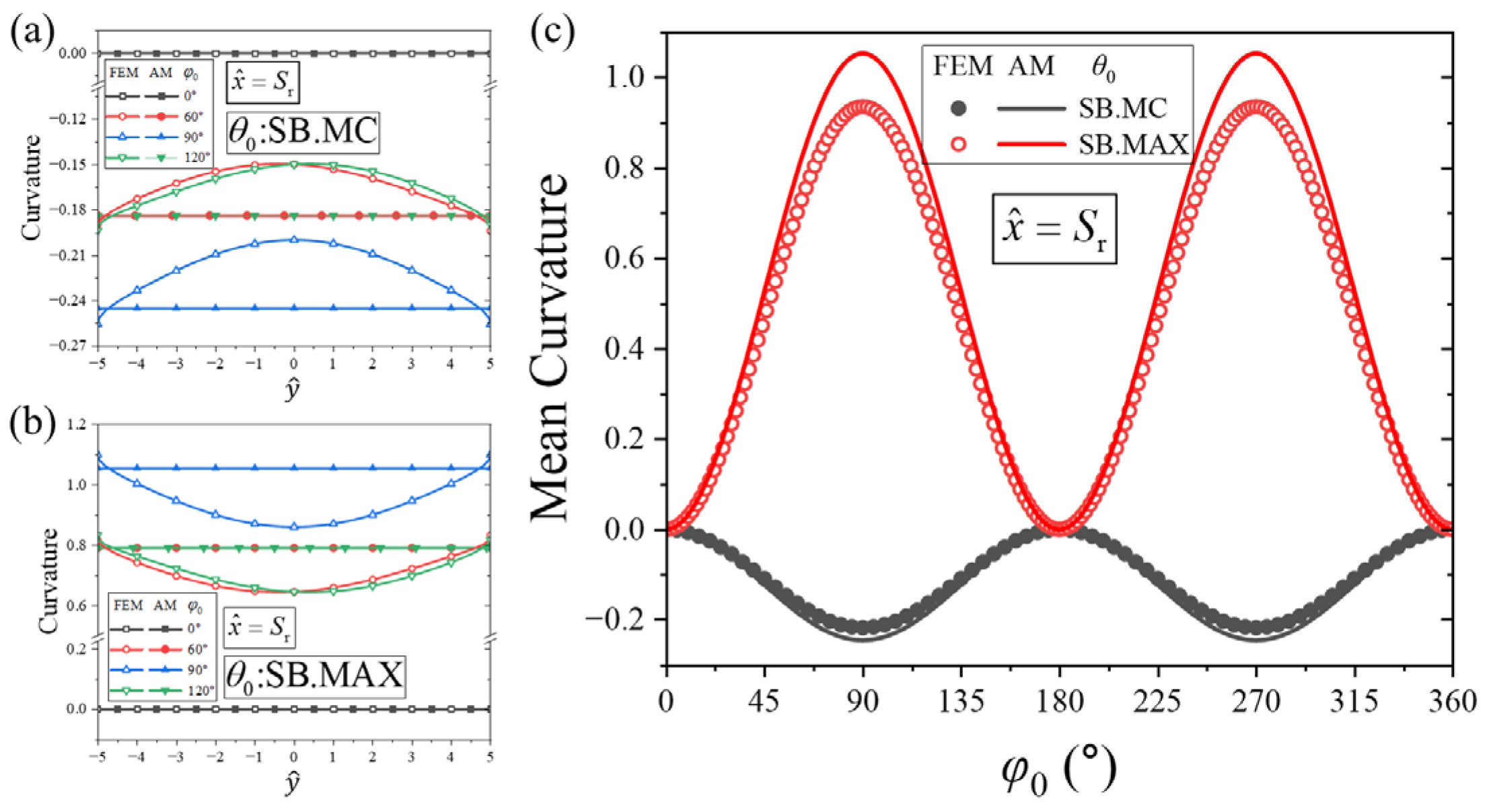
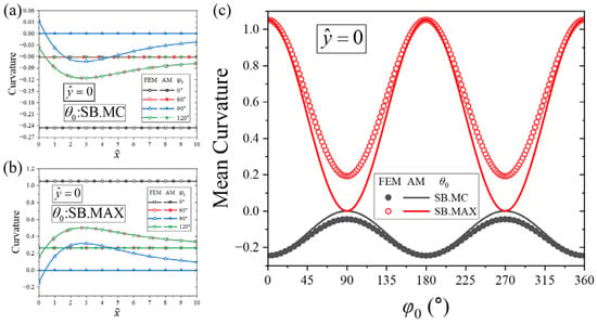
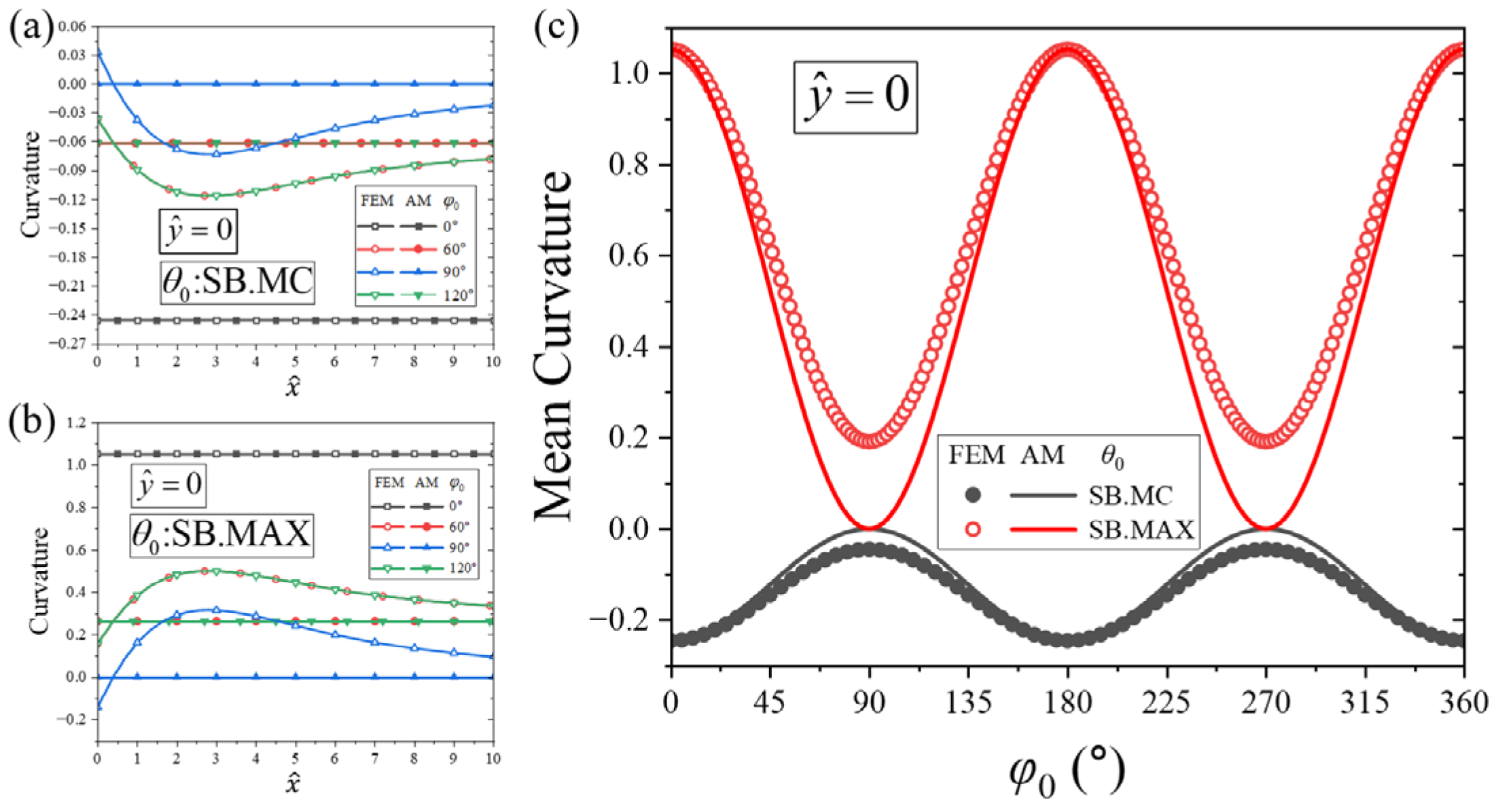
For the sheet, of which the clamped side is generally not perpendicular to the direction which the sheet bends freely in, the sheet no longer exhibits simple unidirectional bending, but more complex multi-directional bending, as shown in Figure 6b–d,f–h. Nevertheless, near the free edge opposite to the clamped boundary, the sheet deforms relatively freely, with its non-zero principal curvature direction aligned with the angle . Consequently, the deflection profile along the free edge, , is non-uniform as shown in Figure 7b,d. The curvature along this free edge, , closely tracks the spontaneous curvature component (29), as shown in Figure 8a,b. The mean value of this free-edge curvature matches which varies periodically with respect to with a period of due to the nematic symmetry of the material as shown in Figure 8c. Similarly, the curvature evaluated along the center line, , fluctuates around the spontaneous curvature component (29) as shown in Figure 9a,b, whose mean value also varies periodically with respect to with a period of as shown in Figure 9c.
Figure 8.
Curvature of the free side of cantilever SB sheets. The approximate solution of the curvature obtained by AM is the spontaneous curvature . (a) Transverse curvature along for SB.MC alignment; (b) Transverse curvature along for SB.MAX alignment; (c) Mean curvature of free edge as a periodic function of for SB.MC and SB.MAX configurations.
Figure 9.
Curvature of the free side of cantilever SB sheets. The approximate solution of the curvature obtained by AM is the spontaneous curvature . (a) Longitudinal curvature along for SB.MC alignment; (b) Longitudinal curvature along for SB.MAX alignment; (c) Mean curvature at the midline as a periodic function of for SB.MC and SB.MAX configurations.
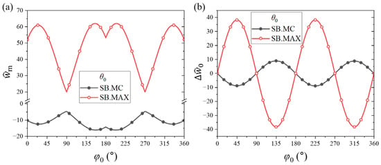
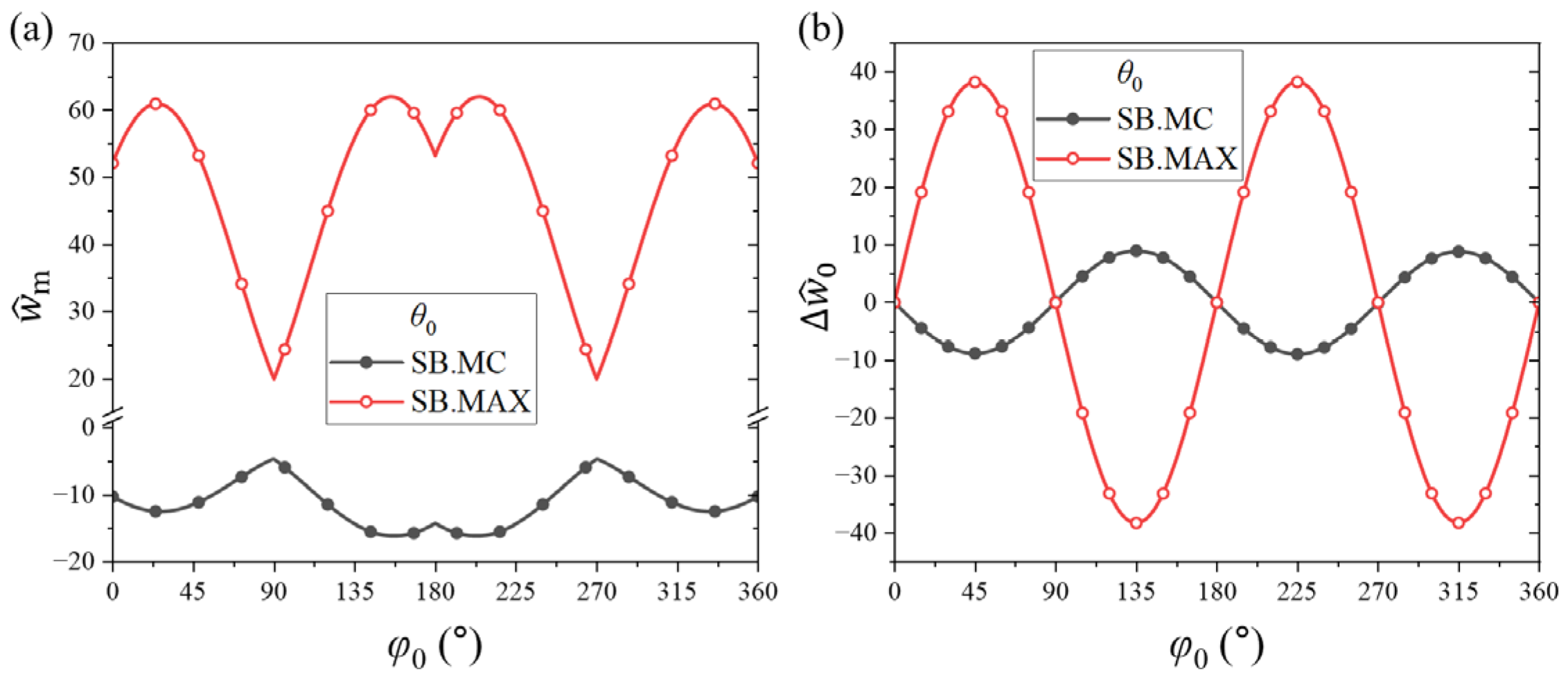
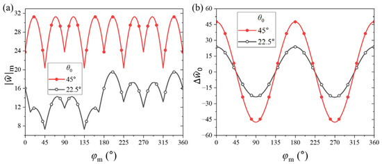
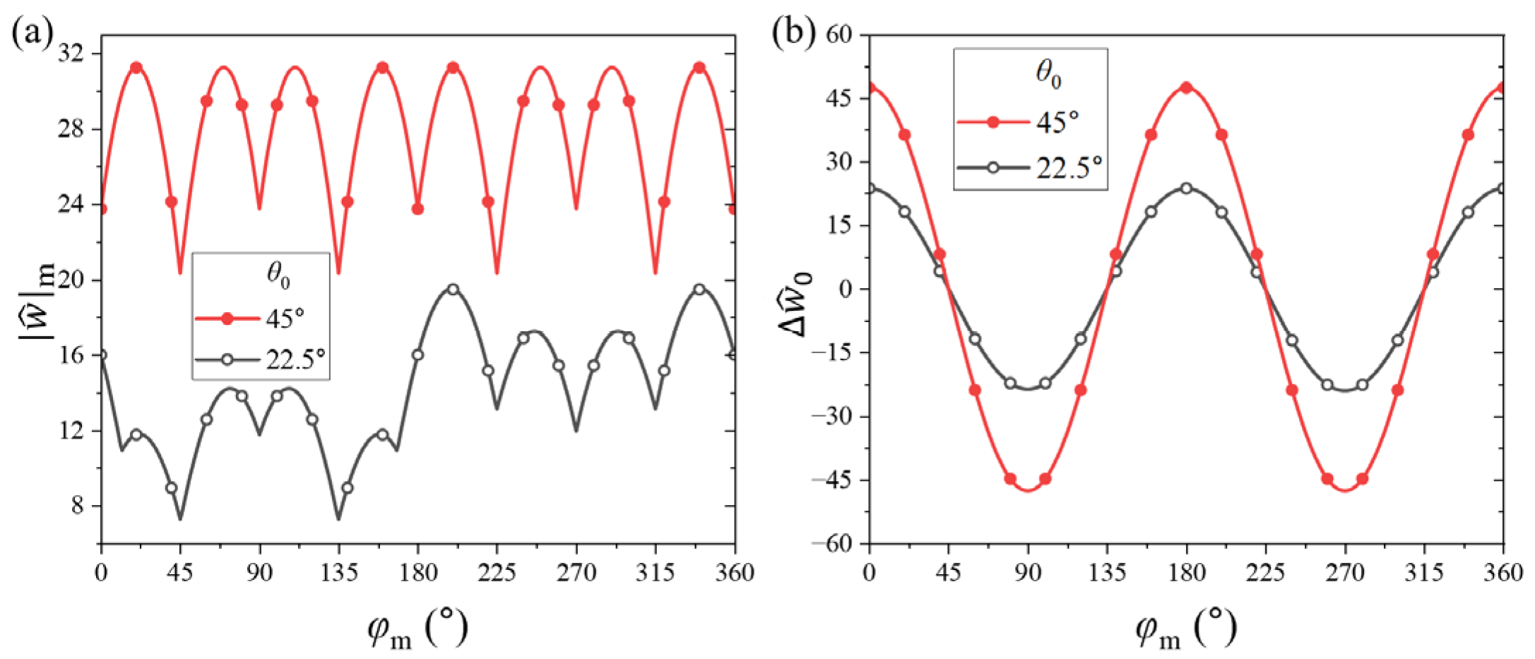
Furthermore, as seen in Figure 6 and Figure 7b,d, when the principal curvature direction is not orthogonal to the clamped edge, i.e., , the deflection varies roughly monotonically with respect to . This causes the deformed free edge to exhibit an overall out-of-plane tilt relative to its initial unbent state. This edge tilting shifts the location of the maximum deflection toward one of the corners of the free edge (i.e., or ), which can render even larger than that produced by the unidirectional bending cases where , as shown in Figure 10a. To quantify this out-of-plane tilt, we define the deflection difference between the two free corners as . As shown in Figure 10b, fluctuates with respect to as a periodic trigonometric function with a period of . Notably, reaches its extreme values at , meaning that the free edge tilts most significantly when the angle between the spontaneous principal curvature direction (32) and the clamped side is exactly . However, this maximum tilt configuration does not yield the largest absolute deflection as shown in Figure 10a,b, indicating that is not positively correlated with the maximum sheet deflection . Specifically, and cannot simultaneously reach their maximum values by tuning alone. Likewise, comparing Figure 8c and Figure 10b shows that is also not positively correlated with the local curvature component , which peaks at , even though they share the identical operating period.
Figure 10.
(a) The maximum deflection of the cantilevered SB sheets, which is at one end of the free side. (b) Deflection difference between two ends of the free side, which can be used to represent the tilt degree of the free side.
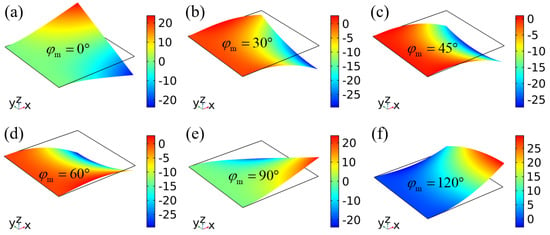
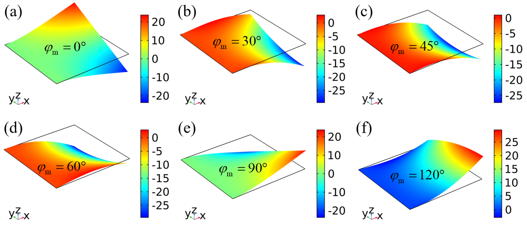
We next consider cantilever sheets with negative spontaneous Gaussian curvature encoded by TB director alignments. As shown in Figure 11, the sheets exhibit complex multi-directional bending while maintaining their characteristic saddle morphology.
Figure 11.
Bending of cantilever sheets with TB director orientation alignments. The orientation , and the orientation gradient . (a) Deformation contour at mid-plane azimuthal angle ; (b) Deformation contour at mid-plane azimuthal angle ; (c) Deformation contour at mid-plane azimuthal angle ; (d) Deformation contour at mid-plane azimuthal angle ; (e) Deformation contour at mid-plane azimuthal angle ; (f) Deformation contour at mid-plane azimuthal angle . Color bar denotes dimensionless deflection .
Figure 12 plots the deflection at the midpoint and the two corners of the free edge, namely and . The midpoint deflection is positively correlated with the spontaneous curvature component (33), which scales proportionally with . The variation in the corner deflections with respect to differs slightly in phase and amplitude from that of the midpoint deflection. Although the maximum deflection of the cantilever sheet does not always occur exactly at the corners, we select the larger value between to represent the peak deflection capability in Figure 13a. The red curve in Figure 13a corresponds to the optimized TB configuration (with and a through-thickness azimuthal gradient ), where the spontaneous principal curvatures and Gaussian curvature (35) reach their mathematical limits, placing it at the highest deflection level in the plot. Moreover, as shown in Figure 11, the right free edge also develops an overall tilt when the principal curvature direction (the orientation from Equation (36)) is oblique to the clamped boundary. We again adopt the corner deflection difference to characterize this tilt behavior as shown in Figure 13b. A more negative spontaneous Gaussian curvature directly amplifies the out-of-plane tilt magnitude. Similar to the SB case, reaches its extreme values at , showing that the free edge tilts most significantly when the principal curvature axis forms a angle with the clamped boundary. Comparing the red curves in Figure 10b and Figure 13b shows that the tilt magnitude generated by the optimized TB alignment (highly negative Gaussian curvature) can exceed that produced by the optimized SB.MAX alignment (maximum principal curvature with zero Gaussian curvature), even though the absolute maximum deflection of the former is generally lower than that of the latter (cf. Figure 10a and Figure 13a).
Figure 12.
Deflection at the end and midpoint of the free side of the cantilever TB sheets. (a) , (b) . The solid and dashed lines are plotted by FEM based on RM and KL plate theories, respectively.
Figure 13.
(a) The larger deflection at both ends of the free edge of cantilevered TB sheets. (b) Deflection difference between two ends of the free side.
3.3. Effects of Spontaneous Shear Strain on Bending of Cantilever Sheets
As established in Section 2.2, the electric-field-strain effect on bending of DLCE sheets collectively driven by the spontaneous curvatures and equivalent spontaneous transverse shear strains . Consequently, the spontaneous shear strain inherently influences the overall bending and deflection profiles, a feature that is also captured by the analytical solutions given by Equations (37) and (44). According to Equation (37), the deflection of cantilever sheets with a completely uniform director distribution is driven solely by the spontaneous shear strain, as detailed in Section 3.1.
Furthermore, for cantilever sheets featuring SB and TB director profiles, we can isolate the role of the shear effect by comparing our RM results with solutions derived from the KL plate theory (plotted as the dashed lines in Figure 7 and Figure 12), which systematically ignores transverse shear strains. The deviation between the KL and RM solutions scales directly with the magnitude of the spontaneous shear strain (24),
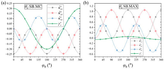
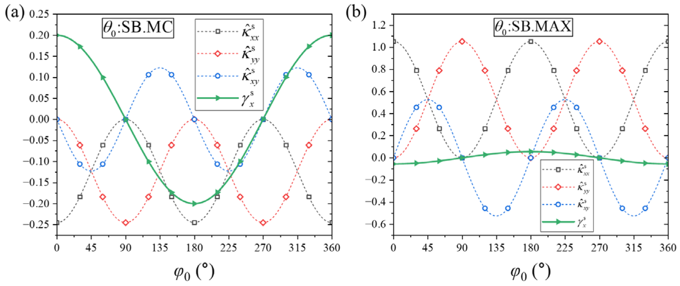
Specifically, in SB cases, the ratios of the spontaneous shear strain to the spontaneous curvatures are generally relatively large for the SB.MC case as shown in Figure 14a. As a result, the discrepancy between the KL and RM predictions is highly pronounced as seen in Figure 7a,b. Conversely, for the SB.MAX configuration, the ratios are remarkably small as shown in Figure 14b, meaning the shear effect is suppressed and the RM solutions converge closely onto the KL curves as seen in Figure 7c,d. Due to material nematic symmetry, the minimum positive period of the spontaneous curvatures (29) with respect to is , satisfying the symmetry relations and . Under ideal geometric and constraint symmetry, the deflection curves predicted by the shear-free KL theory at and exhibit clear symmetric counterparts. Specifically, the longitudinal deflection profiles of the KL solution at and are completely identical as shown by the dashed lines in Figure 7a,c, while the transverse deflection profile at maps perfectly onto at as shown by the dashed lines in Figure 7b,d.
Figure 14.
Comparison of the equivalent spontaneous shear strain and spontaneous curvatures encoded by SB director orientation alignments. Quantitative comparison between equivalent spontaneous transverse shear strain and three components of spontaneous curvature tensor under varying azimuthal angle . (a) Strain and curvature curves for SB.MC alignment ; (b) Strain and curvature curves for SB.MAX alignment .
However, Equation (46) shows that the minimum positive period of the spontaneous shear strain with respect to is , obeying the anti-symmetric relation . This mismatch in angular periodicity breaks the symmetry between the deflection profiles at and when shear is accounted for, which explains the distinct splitting observed in the solid lines of the RM solutions in Figure 7a,b. Further, in the SB.MC case, at and as shown in Figure 14a, meaning the spontaneous shear strain counteracts a portion of the downward bending, resulting in the corresponding downward deflections of the RM solutions being less than that of the KL solutions as shown in Figure 7a,b. Conversely, at , which amplifies the downward deformation and drives the RM deflection beyond the KL baseline. At , , causing the RM and KL curves to overlap perfectly.
Finally, the bending of the cantilever sheets with TB alignments is similarly affected by the spontaneous shear strain. In TB cases, the equivalent spontaneous shear strain (46) reads
where the condition that is a liner function as (28) has been used in the second equation. It is evident from Equation (47) that reaches its peak value at and vanishes identically at . This explicit dependency explains why the KL and RM solutions are perfectly identical for the case but diverge significantly when as illustrated in Figure 12.
4. Conclusions
This study establishes a rigorous theoretical framework to investigate the electro-mechanical bending mechanics of cantilevered DLCE sheets. Utilizing the Reissner-Mindlin plate theory, the active deformation driven by the electric-field-induced rotation of nematic mesogens is mathematically formulated as macroscopic spontaneous curvatures and equivalent spontaneous transverse shear strains. We demonstrate that the bending morphology is deterministically governed by the through-thickness gradient of the director alignment. Specifically, by engineering distinct microstructural layouts, such as splay-bend and twist-bend alignments, specific spontaneous Gaussian and principal curvatures can be intricately encoded into the flat sheet, allowing for highly programmable macroscopic shape morphing.
Furthermore, the synergistic interplay between these tailored spontaneous curvatures and the asymmetric clamped boundary constraints generates a rich variety of three-dimensional configurations, featuring targeted free-end deflections and out-of-plane tilting. Our analysis reveals that while splay-bend alignments excel in maximizing the global bending deflection, twist-bend configurations are superior for achieving a pronounced free-edge tilt. By systematically tailoring the principal bending directions via director alignment, the global deformation kinematics can be actively regulated. Notably, we uncover a universal geometric rule: the maximum free-edge tilt of the cantilevered sheet is consistently achieved when the principal axis of spontaneous curvature is oriented at exactly 45 degrees relative to the clamped boundary.
Beyond this curvature-dominated morphing, we explicitly highlight the critical, yet often overlooked, role of the spontaneous transverse shear strain, which significantly influences the overall bending profile even within the thin-plate limit. Due to the inherent nematic symmetry of the material, the spatial periodicity of the spontaneous shear strain inherently differs from that of the spontaneous curvature. This periodic mismatch introduces a non-trivial symmetry-breaking effect that fundamentally alters the deflection rules predicted by classical curvature-only models.
It is worth noting that the present theoretical framework inherently involves dual applicability boundaries dictated by its foundational assumptions. First, regarding the localized multi-field coupling, the analytical approximations are derived under the assumption of a relatively weak electrical excitation (see Appendix B). The physical threshold for a “weak” excitation is not absolute, but fundamentally depends on the intrinsic material parameters (e.g., the elastic constraint and dielectric anisotropy). Second, from a structural mechanics perspective, the RM plate model is formulated under the small-strain assumption. We emphasize that this linearized kinematic model primarily serves as an efficient and physically transparent tool for qualitative analysis and providing morphological design insights, rather than for highly non-linear quantitative predictions under extreme fields. Its applicability requires the macroscopic deformation to remain within the geometrically linear regime. Under exceptionally high electric fields or in extreme actuation regimes where non-linear geometric effects become dominant, a fully non-linear finite deformation formulation would be required.
Nevertheless, collectively, these theoretical insights establish a robust mechanical foundation for understanding anisotropic electro-actuation, providing quantitative guidance for the structural design of DLCE-based directional soft actuators, programmable sensors, and flexible devices.
Author Contributions
H.W.: Investigation, formal analysis, and writing—original draft. Y.X.: Conceptualization, methodology, validation, and writing—reviewing and editing. All authors have read and agreed to the published version of the manuscript.
Funding
This work is supported by the National Natural Science Foundation of China (Grant No. 12202076) and the Key Discipline Innovation Project in Civil Engineering at Changsha University of Science and Technology (Grant No. 23ZDXK03).
Data Availability Statement
Data will be made available upon request.
Conflicts of Interest
The authors declared that they have no conflicts of interest with respect to this work.
Appendix A. Formulation of the Electro-Mechanical-Director Coupling
This section details the derivation of the governing equations and constitutive relations for the coupled mechanical-electrical-director system based on the principle of virtual work. At thermodynamic equilibrium, the variation in the total free energy equals the virtual mechanical work minus the virtual electrical complementary work, satisfying the following variational statement:
where represents the coupled free energy density, which explicitly depends on the strain tensor , the electric field , as well as the current and initial director fields, and , respectively. Here, t denotes the surface traction, u is the mechanical displacement, q is the surface free charge density, and is the electric potential such that . Taking the variations in the state variables into account, the variation in the free energy density is expressed as
Applying the divergence theorem and integration by parts, the volume integral of Equation (A2) can be expanded into
where the Cauchy stress tensor and the electric displacement vector D are thermodynamically defined as
Substituting Equation (A3) into Equation (A1) yields
To ensure that the above variational equation holds identically for any kinematically admissible virtual variations , , and , the following three independent equilibrium equations must be satisfied. The mechanical equilibrium equation is as follows:
with boundary conditions or prescribed . The electrostatic Maxwell’s equation is as follows:
with boundary conditions or prescribed . Finally, the equilibrium equations for the director orientation are as follows:
Physically, Equation (A8) implies that the generalized thermodynamic force acting on the director must be collinear with d. This arises from the constraint that d is a unit vector, meaning its admissible virtual variation must be orthogonal to d, i.e., .
To proceed, the total free energy density is additively decomposed into an elastic component and an electrical Gibbs component:
which are phenomenologically formulated as
Here, C is the fourth-order elasticity tensor, is the spontaneous strain defined by Equation (1), and k acts as a penalty parameter governing the reorientation of the director d deviation from its initial state . The anisotropic dielectric tensor is , with and representing the permittivities parallel and perpendicular to d. Combining Equations (A9) and (A10), the electromechanical constitutive relations given by Equation (A4) are derived as
Correspondingly, the director equilibrium Equation (A8) takes the explicit form:
This rigorously establishes the 3D multi-field coupled boundary-value problem, laying the fundamental groundwork for the subsequent asymptotic analysis.
Appendix B. Asymptotic Analysis of Director Reorientation and the Reduced Spontaneous Strain
We now investigate the regime of small director reorientations induced by a weak electric field. Assuming that the electrostatic torque dominates the director reorientation process, the passive mechanical stress term in Equation (A12) can be neglected as a leading-order approximation. The director equilibrium equation then reduces to the following dimensionless form:
where is the dimensionless equivalent electric field. Let the current director be perturbed as . Under the assumption of small reorientations, the variation , which inherently requires a weak actuating field, . To establish the scaling relation, Equation (A13) is rearranged as
A scaling analysis reveals that . To obtain an analytical solution for , terms of and higher are truncated. Consequently, the left-hand side of Equation (A14) is approximated as . Given that d remains a unit vector, this constraint requires , leading to . Thus, Equation (A14) is linearized to
Since the cross product vanishes, the term within the parentheses must be collinear with :
Taking the inner product of Equation (A16) with and utilizing the orthogonality relation yields the scalar multiplier . Substituting this back provides the explicit analytical expression for the director increment:
This indicates that the reoriented director is strictly confined to the plane spanned by and .
Within this small director reorientation framework, the spontaneous strain tensor given by Equation (1) can be linearized with respect to :
Substitution of Equation (A17) into Equation (A18) reveals that the local spontaneous strain degenerates into a plane strain state within the principal plane formed by and . For a sheet subjected to a through-thickness voltage, it is kinematically consistent to assume an out-of-plane electric field. As illustrated in Figure 1b, the principal plane aligns with the local plane. Defining the initial director in the local frame as , its global representation is , with given by Equation (6). Since the local and global frames share the z-axis, the local electric field satisfies . Applying the tensor transformation yields
where the spontaneous strain in the local frame is
Substituting and into Equation (A20), the explicit matrix form is obtained as
where the true electric field relates to the dimensionless counterpart via . Thus, the analytical expressions for the electroactive spontaneous strain, corresponding exactly to Equations (2) and (3) in the main text, are rigorously validated.
Appendix C. Analytical Approximate of the Through-Thickness Electric Field
Under the aforementioned approximations of a weak electric field and small director reorientation, the constitutive relation for the electric displacement given by Equation (A11) simplifies to
Given that the designed initial director field is exclusively a function of the thickness coordinate z, it is a justified assumption that the electric field E, and consequently D (A22), are primarily 1D functions of z. Under this condition, the electrostatic Maxwell’s Equation (A7) simplifies to a one-dimensional differential equation:
where is the transverse component of D, and the effective permittivity is defined in Equation (5). Expressing the electric field as the negative gradient of the potential, i.e., , integrating Equation (A23) along the thickness yields
where and are integration constants determined by the potentiostatic boundary conditions at the compliant electrodes:
Enforcing these boundary conditions yields , where is thickness-averaged permittivity given by Equation (5) and is the nominal applied electric field. Substituting back into Equation (A24) and differentiating with respect to z recovers the exact analytical expression for the local electric field intensity E, identical to Equation (4) utilized in the main text.
Appendix D. Verification of the Approximate Analytical Solutions via the 3D Finite Element Analysis
To corroborate the theoretical approximations derived in Appendix B and Appendix C, a comprehensive 3D finite element analysis is conducted based on the coupled mechanical-electrical-director framework derived in Appendix A. Within the COMSOL Multiphysics environment, the Solid Mechanics, Electrostatics, and Mathematics modules were simultaneously solved to fully capture the coupling among Equations (A6)–(A8).
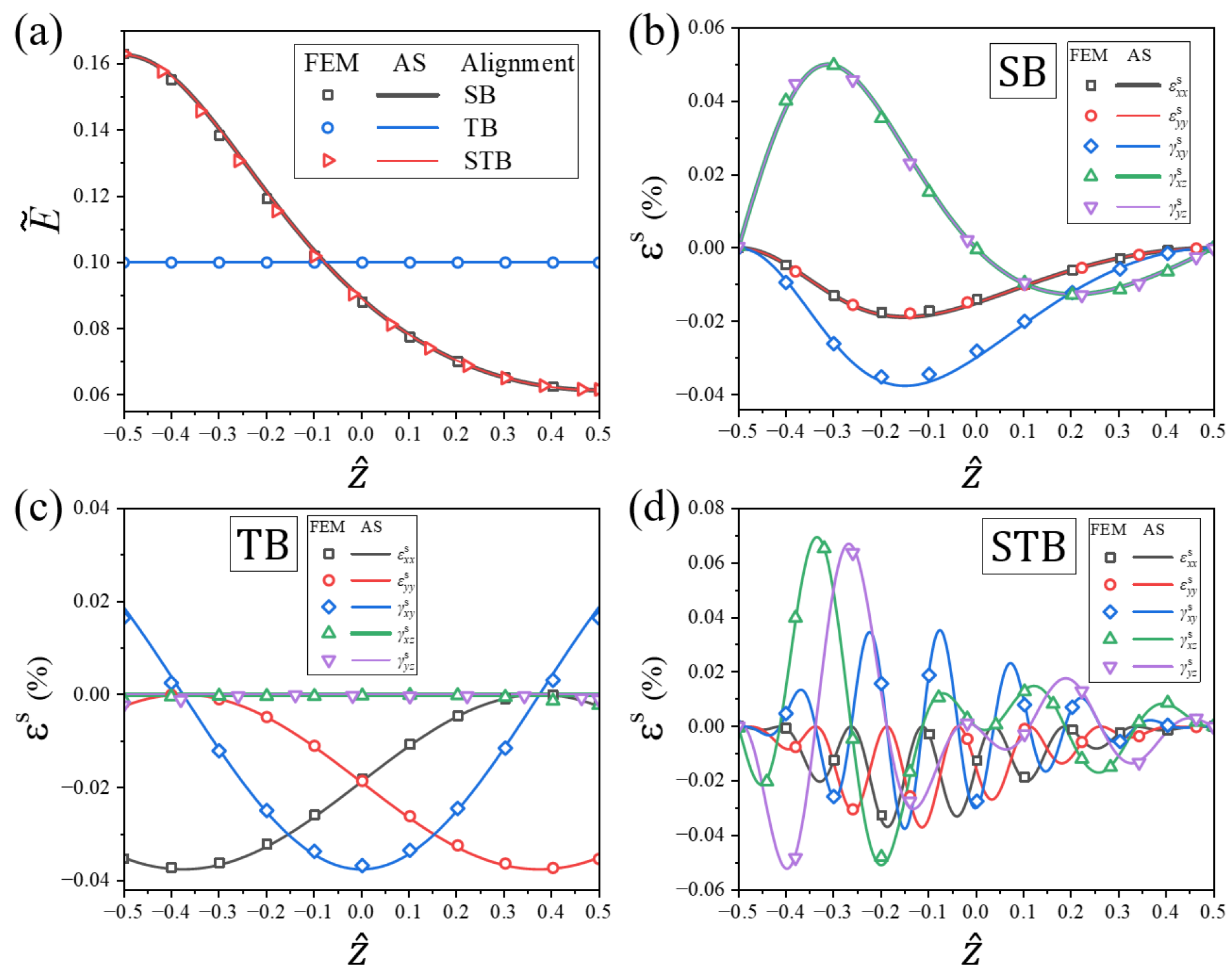
Free-standing DLCE sheets programmed with representative SB, TB, and splay- STB initial alignments were simulated under electro-actuation. As depicted in Figure A1, the simulated bending morphologies perfectly reproduce the macroscopic deformations predicted by the reduced plate theory (Figure 3 in the main text), validating the macroscopic emergence of zero, negative, and positive Gaussian curvatures, respectively. The contour plots of the effective electric potential and the vector field of in Figure A1 confirm that the internal electric field acts predominantly along the thickness direction, which strongly supports the 1D field assumption utilized in Appendix B and Appendix C. Figure A2a quantitatively compares the through-thickness electric field distributions. As analytically prescribed by Equations (4) and (5), the magnitude of E is solely dictated by the out-of-plane tilt gradient , regardless of the azimuthal twist . This is verified by the uniform E-field in the TB sample (where is constant) and the identical non-uniform profiles for the SB and STB samples (which share the same gradient). The finite element scatter data align flawlessly with the analytical curves. Furthermore, Figure A2b–d detail the complex, non-linear spontaneous strain profiles across the thickness. Notably, the high azimuthal gradient in the STB alignment induces rapid oscillatory variations in the strain components. Across all programmed director alignments, the closed-form analytical solutions of Equation (14) demonstrate excellent quantitative agreement with the full 3D finite element numerical results.
Figure A1.
3D finite element simulations of electric-field-induced deformations of free-standing DLCE sheets with distinct initial director alignments: (a) SB alignment exhibiting zero Gaussian curvature; (b) TB alignment exhibiting negative Gaussian curvature; and (c) STB alignment exhibiting positive Gaussian curvature. The color contours denote the electric potential distribution, and the arrows represent the local electric field vectors. The applied nominal electric field is .
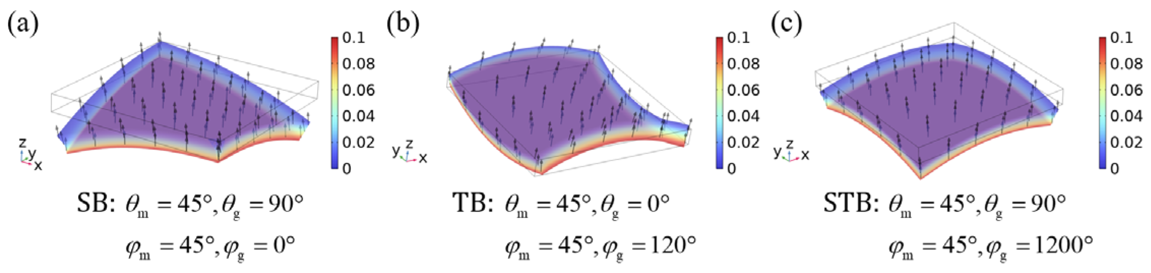
Figure A2.
Quantitative comparison between the analytical solutions (AS, solid lines) and 3D finite element solutions (FEM, scatter dots) along the normalized thickness coordinate : (a) through-thickness distributions of the dimensionless equivalent electric field intensity for SB, TB, and STB alignments; and the corresponding through-thickness profiles of the electrocactive spontaneous strain components for the (b) SB, (c) TB, and (d) STB alignments.
In conclusion, the 3D numerical results systematically validate the reliability and high accuracy of the analytical approximations. This comprehensive verification fully justifies their implementation in the macroscopic plate modeling, confirming that within the intended operational regime of relatively weak electrical excitation, the proposed analytical framework serves as a highly reliable and physically transparent tool for the morphological design of DLCE sheets.
References
- White, T.J.; Broer, D.J. Programmable and adaptive mechanics with liquid crystal polymer networks and elastomers. Nat. Mater. 2015, 14, 1087–1098. [Google Scholar] [CrossRef] [Scilit] [PubMed]
- Sun, D.; Zhang, J.; Li, H.; Shi, Z.; Meng, Q.; Liu, S.; Chen, J.; Liu, X. Toward application of liquid crystalline elastomer for smart robotics: State of the art and challenges. Polymers 2021, 13, 1889. [Google Scholar] [CrossRef] [Scilit]
- Zhai, Y.C.; Tolley, M.T.; Ng, T.N. Digital programming of liquid crystal elastomers to achieve high-fidelity surface morphing. Appl. Mater. Today 2022, 27, 101501. [Google Scholar] [CrossRef] [Scilit]
- Warner, M.; Terentjev, E. Liquid Crystal Elastomers; Oxford University Press: Oxford, UK, 2007. [Google Scholar]
- Mistry, D.; Traugutt, N.A.; Yu, K.; Yakacki, C.M. Processing and reprocessing liquid crystal elastomer actuators. J. Appl. Phys. 2021, 129, 140901. [Google Scholar] [CrossRef] [Scilit]
- Chen, J.; Johnson, A.S.; Weber, J.; Akomolafe, O.I.; Jiang, J.; Peng, C. Programmable light-driven liquid crystal elastomer kirigami with controlled molecular orientations. Adv. Intell. Syst. 2022, 4, 2100233. [Google Scholar] [CrossRef] [Scilit]
- Fukunaga, A.; Urayama, K.; Takigawa, T.; DeSimone, A.; Teresi, L. Dynamics of electro-opto-mechanical effects in swollen nematic elastomers. Macromolecules 2008, 41, 9389–9396. [Google Scholar] [CrossRef] [Scilit]
- Urayama, K.; Honda, S.; Takigawa, T. Deformation coupled to director rotation in swollen nematic elastomers under electric fields. Macromolecules 2006, 39, 1943–1949. [Google Scholar] [CrossRef] [Scilit]
- Kim, K.; Guo, Y.; Bae, J.; Choi, S.; Song, H.Y.; Park, S.; Hyun, K.; Ahn, S. 4D Printing of Hygroscopic Liquid Crystal Elastomer Actuators. Small 2021, 17, e2100910. [Google Scholar] [CrossRef] [Scilit] [PubMed]
- Davidson, Z.S.; Shahsavan, H.; Aghakhani, A.; Guo, Y.; Hines, L.; Xia, Y.; Yang, S.; Sitti, M. Monolithic shape-programmable dielectric liquid crystal elastomer actuators. Sci. Adv. 2019, 5, eaay0855. [Google Scholar] [CrossRef] [Scilit] [PubMed]
- Aharoni, H.; Xia, Y.; Zhang, X.Y.; Kamien, R.D.; Yang, S. Universal inverse design of surfaces with thin nematic elastomer sheets. Proc. Natl. Acad. Sci. USA 2018, 115, 7206–7211. [Google Scholar] [CrossRef] [Scilit] [PubMed]
- Zhao, J.; Zhang, L.; Hu, J. Varied alignment methods and versatile actuations for liquid crystal elastomers: A Review. Adv. Intell. Syst. 2021, 4, 2100065. [Google Scholar] [CrossRef] [Scilit]
- Ula, S.W.; Traugutt, N.A.; Volpe, R.H.; Patel, R.R.; Yu, K.; Yakacki, C.M. Liquid crystal elastomers: An introduction and review of emerging technologies. Liq. Cryst. Rev. 2018, 6, 78–107. [Google Scholar] [CrossRef] [Scilit]
- Zeng, H.; Wani, O.M.; Wasylczyk, P.; Kaczmarek, R.; Priimagi, A. Self-regulating iris based on light-actuated liquid crystal elastomer. Adv. Mater. 2017, 29, 1701814. [Google Scholar] [CrossRef] [Scilit]
- Barnes, M.; Verduzco, R. Direct shape programming of liquid crystal elastomers. Soft Matter 2019, 15, 870–879. [Google Scholar] [CrossRef] [Scilit] [PubMed]
- Camacho-Lopez, M.; Finkelmann, H.; Palffy-Muhoray, P.; Shelley, M. Fast liquid-crystal elastomer swims into the dark. Nat. Mater. 2004, 3, 307–310. [Google Scholar] [CrossRef] [Scilit] [PubMed]
- Fowler, H.E.; Rothemund, P.; Keplinger, C.; White, T.J. Liquid crystal elastomers with enhanced directional actuation to electric fields. Adv. Mater. 2021, 33, e2103806. [Google Scholar] [CrossRef] [Scilit] [PubMed]
- Xu, Y.; Shen, Y.; Huo, Y.; Xu, F. Spontaneous shear strain governed bending of dielectric nematic elastomer sheets with in-plane director orientation gradients. J. Appl. Mech. 2025, 92, 071007. [Google Scholar] [CrossRef] [Scilit]
- Qiu, W.; Xu, Y.; Xu, F.; Huo, Y. Programmable electric-field-induced bending shapes of dielectric liquid crystal elastomer sheets. Extrem. Mech. Lett. 2023, 60, 101982. [Google Scholar] [CrossRef] [Scilit]
- Xu, Y.; Zhang, Y.; Huo, Y. Electric-field induced deformation and bending in nematic elastomer strips with orientation gradient. Int. J. Solids Struct. 2020, 202, 243–259. [Google Scholar] [CrossRef] [Scilit]
- Xu, Y.; Gong, S. Anisotropic electro-mechanical-orientational coupling deformation of dielectric nematic elastomers: Modeling and analysis. Int. J. Solids Struct. 2026, 330, 113876. [Google Scholar] [CrossRef] [Scilit]
- Wang, T.S.; Farajollahi, M.; Choi, Y.S.; Lin, I.-T.; Marshall, J.E.; Thompson, N.M.; Kar-Narayan, S.; Madden, J.D.; Smoukov, S.K. Electroactive polymers for sensing. Interface Focus 2016, 6, 19. [Google Scholar] [CrossRef] [Scilit]
- Lu, T.; Ma, C.; Wang, T. Mechanics of dielectric elastomer structures: A review. Extrem. Mech. Lett. 2020, 38, 100752. [Google Scholar] [CrossRef] [Scilit]
- Zhang, Y.; Huo, Y. First order shear strain beam theory for spontaneous bending of liquid crystal polymer strips. Int. J. Solids Struct. 2018, 136–137, 168–185. [Google Scholar] [CrossRef] [Scilit]
- Zhao, D.; Liu, Y. Light-induced spontaneous bending of a simply supported liquid crystal elastomer rectangular plate. Phys. Rev. E 2020, 101, 042701. [Google Scholar] [CrossRef] [Scilit] [PubMed]
- Wang, C.M.; Reddy, J.N.; Lee, K.H. Shear Deformable Beams and Plates; Elsevier Science: Amsterdam, The Netherlands, 2000. [Google Scholar]
- Sawa, Y.; Urayama, K.; Takigawa, T.; DeSimone, A.; Teresi, L. Thermally Driven Giant Bending of Liquid Crystal Elastomer Films with Hybrid Alignment. Macromolecules 2010, 43, 4362–4369. [Google Scholar] [CrossRef] [Scilit]
Disclaimer/Publisher’s Note: The statements, opinions and data contained in all publications are solely those of the individual author(s) and contributor(s) and not of MDPI and/or the editor(s). MDPI and/or the editor(s) disclaim responsibility for any injury to people or property resulting from any ideas, methods, instructions or products referred to in the content. |
© 2026 by the authors. Licensee MDPI, Basel, Switzerland. This article is an open access article distributed under the terms and conditions of the Creative Commons Attribution (CC BY) license.