


Abstract
In this paper, we investigate the absolute stability of several Translationally Invariant Configurations (TICs) observed in cholesteric liquid crystal samples. The bounding plates of the samples may impose homeotropic anchoring (case 1), slightly tilted anchoring when the plates are also rubbed in either the same (case 2) or opposite (case 3) directions, or hybrid anchoring with planar on one plate and homeotropic on the other. In each case, the stability is examined as a function of the confinement ratio—defined as the ratio of the sample thickness to the cholesteric pitch—and of the applied field (electric and/or magnetic).
1. Introduction
When a nematic liquid crystal is doped with a chiral molecule, one obtains a cholesteric phase in which the director field is naturally twisted in a single direction. The distance P over which the director rotates by is called the cholesteric pitch, and the equilibrium twist is given by . This equilibrium rotation of the director gives rise to a layered structure—or, more precisely, a pseudo-layered structure—which endows the cholesteric phase with unique optical properties. The most spectacular and best-known of these consists of remarkable specular reflections from the layers when the pitch is comparable to the wavelength of light [1,2,3]. This property is used, for instance, in the fabrication of color displays [4,5,6,7] and thermometers [8]. The layered structure of the cholesteric phase can also be harnessed in a wide range of sensing applications, including the detection of physical stimuli (temperature, strain/stress), chemical species (volatile organic compounds, ions, pH), and biological targets (biomarkers, pathogens) [9].
In this paper, we consider a cholesteric phase confined between two parallel glass plates that impose fixed anchoring directions for the director. The anchoring may be normal (or homeotropic)—possibly slightly tilted in a given direction if the plates are rubbed—or planar. These boundary conditions are often incompatible with the helical structure of the phase, leading to frustration. In that case, it is necessary to deform the helical director field in the bulk in order to match the surface constraints. In extreme cases, this frustration may lead to a complete unwinding of the cholesteric helix.
This occurs in particular when the plates impose homeotropic anchoring and the sample thickness is typically smaller than the cholesteric pitch. The cholesteric then completely unwinds, forming a homeotropic nematic phase. As the thickness increases, the cholesteric structure reappears, most often in the form of characteristic finger textures [2,10,11,12,13,14]. It is also possible to restore the cholesteric phase by applying an electric field to the homeotropic nematic phase (i.e., to the unwound cholesteric), provided that the liquid crystal has a negative dielectric anisotropy [15]. In this case, experiments show that above a critical field, a texture that is translationally invariant in the plane of the sample develops (the so-called TIC, or Translationally Invariant Configuration), in which the director field twists only in the direction perpendicular to the plates.
This solution, which always appears first after the electric field is applied, is not always stable and may lead to a periodic finger texture. In that case, the director field also twists in the direction perpendicular to the fingers.
In a recent article [16], we studied the TIC solution in detail and showed that it is possible to fix its orientation (given by its -director defined below) by applying a magnetic field in the plane of the sample. This property is particularly interesting for guiding the propagation of active quasiparticles such as torons [17,18] in homeotropic samples [19]. The TIC also exhibits interesting optical properties [20] that can be exploited to design tunable photonic elements and advanced polarization control systems [21].
However, for such applications, the TIC must remain stable. Determining the region of the parameter plane (V, ) in which it is stable can be achieved experimentally by preparing several samples with different thicknesses, but this approach is particularly time-consuming and tedious. An alternative is to analyze numerically the stability of this solution. We previously attempted this approach using the ‘circle model’ on the unit sphere [15]. However, this model proved insufficiently accurate for practical predictions. In particular, it significantly underestimated the extent of the region in the (V, ) parameter plane where the TIC is actually unstable.
In this paper, we revisit this method by using a new ansatz for the director field that is different from the one employed in the circle model. Using this ansatz, we show how to test the stability of the TIC in homeotropic samples at each point of the phase diagram and how to calculate the modulation wavelength when it becomes unstable.
Since this method is very general, we then generalize it to a slightly different geometry in which the surfaces imposing homeotropic anchoring are rubbed in a single direction. We show that rubbing orients the TIC and affects its stability. In this context, we consider two situations depending on whether the plates are rubbed in the same direction or in opposite directions.
Finally, we analyze the case of samples with hybrid anchoring, where the bottom plate imposes planar unidirectional anchoring and the top plate homeotropic anchoring. We show that, under these boundary conditions, a TIC forms and may become unstable above a critical thickness to a stripe instability. The wavelength and orientation of the stripes with respect to the anchoring direction at the bottom plate are also calculated as functions of the confinement ratio and compared with experiments.
2. TIC Stability in Homeotropic Samples
2.1. Basic Properties of the TIC
We consider a cholesteric sample of negative dielectric anisotropy sandwiched between two parallel flat electrodes (glass plates covered with ITO) treated for strong homeotropic anchoring. The bottom electrode is at and the top one at . In the frame (), the director has the following components:
In the TIC, the director field is only twisted along the z direction (perpendicular to the sample plane) so that angles and are only a function of z and time t (in the non-stationary regime). By definition, the -director, which determines the orientation of the TIC in the sample plane, is the unit vector with the following components:
where . It should be noted here that and are not equivalent, as they correspond to two TICs oriented in opposite directions. The reader will also note that the direction of depends on the chosen direction of on the plates. In our case, we will always take on the plates when they are treated for homeotropic anchoring.
The TIC structure is obtained by solving the equations:
where f is the density of free energy and the Rayleigh dissipation function, respectively, given by:
and
In these equations, , and are the splay, twist and bend elastic constants, respectively. is the magnetic anisotropy (positive in our experiments), the magnetic field (parallel to the x-axis), is the electric field (parallel to the z-axis), is the electric displacement, and is the rotational viscosity.
Using these expressions, the dynamical Equation (3) can be written explicitly as follows:
and
where , , , and for any function u.
In these equations, , with U being the electric potential. Because the TIC is translationally invariant in the horizontal plane, the only non-zero component of the displacement field is , where () is the relative dielectric permittivity perpendicular (parallel) to and is the dielectric anisotropy. In the dielectric regime, the potential U must satisfy the Maxwell equation , which reads:
Under homeotropic anchoring, these equations must be solved with the following boundary conditions (BC) on the two electrodes:
where V is the rms-applied voltage. These equations can be easily solved with Mathematica using the Method of Lines, which is a general procedure for finding the solution of time-dependent partial differential equations (for more details, see [16]).
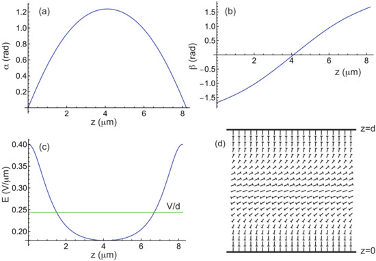
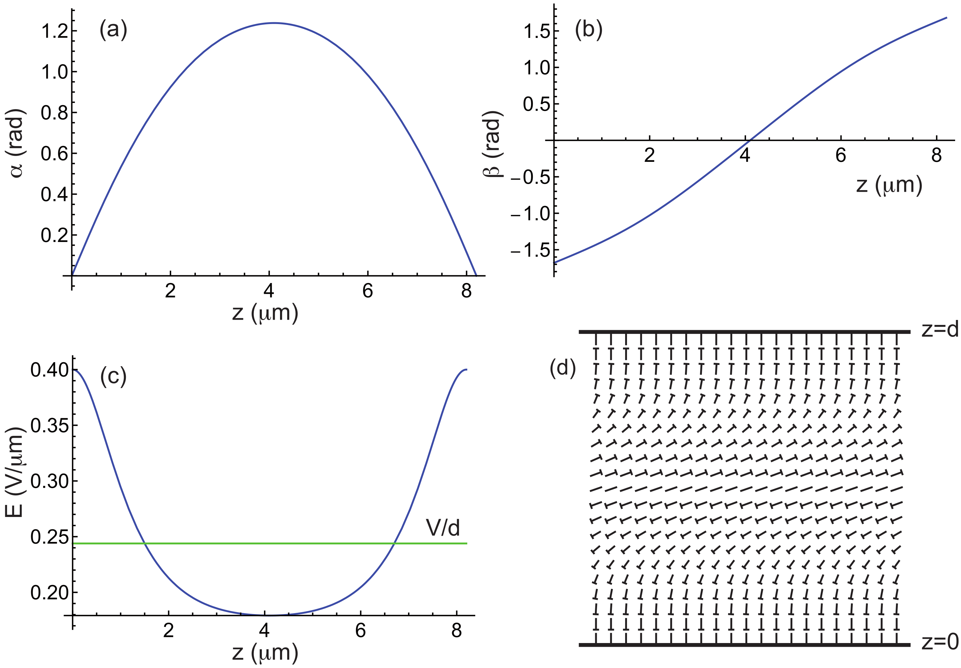
Figure 1 illustrates how the angles and and the electric field E vary inside a TIC in the stationary regime. The director field is also depicted using the nail representation for completeness. In this example, the calculations were carried out for the liquid crystal MLC2079 doped with 0.813 wt% of the chiral molecule R811 (both supplied by Merck), which is the mixture used in our experiments (see below). The material constants of this mixture are listed in Table 1. For this concentration of R811, .
Figure 1.
(a–c) Angles and as well as electric field E as a function of z in a TIC calculated by taking m, m, , , and the material constants of the mixture MLC2079/R811 given in Table 1. In this example, the -director is parallel to the x-axis. (d) Nail diagram of the corresponding director field in the plane. The tip of the nail indicates the part of the molecule oriented toward the observer.
Table 1.
Material constants of the Merck mixture MLC2079. The elastic constants are given in pN, and the viscosity in Pa s. and are the ordinary and extraordinary indices (at nm) [16].
2.2. Stability Analysis of the TIC
When an electric field is applied to the sample, the TIC always appears first, provided that the applied voltage exceeds the critical voltage above which the homeotropic nematic phase destabilizes. We calculated this voltage in [16] as a function of the confinement ratio and the magnetic field B and found:
In these equations
with by setting and .
We now discuss how to destabilize the numerically computed TIC. Experiments show that when , the TIC always modulates with a wave vector parallel to the -director. This type of modulation leads, in the nonlinear regime, to the so-called cholesteric fingers of the first type (also referred to as CF1 in the literature, [2,13]). These fingers are always perpendicular to the TIC (i.e., to the –director of the TIC).
In previous work [2,15,22], we used a rather complex ansatz to describe the director field, based on the ‘circle model’ on the sphere . This model assumes that the director traces circles on the sphere when describing lines parallel to inside the sample. In reality, the trajectories are not circular, and this model does not allow us to predict accurately in which region of the phase diagram the TIC becomes unstable and forms fingers. To overcome this difficulty, we propose a new ansatz for the director field that is both simpler and more general, and which allows us to predict the stability limits of the TIC with much greater accuracy. When the -director is along the x-direction, our ansatz reads:
noting that must be replaced by when the TIC is oriented perpendicular to the x-axis. In the following, we assume that the TIC is parallel to the x-axis and we therefore use Equation (14) in our calculations. In these equations, and are the numerically calculated functions describing the TIC, while the terms proportional to and are perturbative terms. The functions and are unknown, but they must satisfy the boundary conditions
and
under strong homeotropic anchoring.
The next step in determining whether the TIC becomes unstable is to calculate the energy per unit area of the sample:
where , and to expand it as a power series in and . This calculation is straightforward with Mathematica and, to second order in the perturbations, leads to the following expression:
where a, b and c can be expressed as:
where , , etc., are functions of , , and . The calculation shows that . The other functions are given in Appendix A.
The method used to determine when the TIC becomes unstable consists in finding when the curvature of the potential becomes negative at and . This curvature depends on the direction in the plane , which is defined by setting and , and reads (within a factor of 2):
Since the TIC is unstable whenever , one must minimize as a function of k, , , and . To solve this problem, we proceed step by step as follows.
• Step 1: We first expand the functions and in Fourier series, keeping only the first terms compatible with the boundary conditions (15) and (16). This simply gives:
Note that the functions g and h can be normalized by taking and , since they are defined up to a multiplicative constant. With these functions, is minimized numerically using Mathematica as a function of k and . This yields a first set of values and .
• Step 2: With these two values and by taking , we then minimize as a function of . This can be easily achieved by noting that a, b and c can be written in the following form:
where , , etc., are functions of , and whose calculation rules are given in Appendix B. Minimizing as a function of leads to the Euler equation:
where
Solving Equation (23) with the boundary conditions (15) yields a new function , which can be normalized by setting .
• Step 3: This step consists now in minimizing with respect to by taking , and . By writing
where , , etc., are functions of , and whose calculation rules are given in Appendix C, we obtain the following Euler equation:
where
Solving Equation (26) leads to a new function , which can be normalized by setting .
Once this cycle is completed, it can be repeated, starting with a new calculation of k and using the functions and , before recalculating g and h, until convergence is achieved. In practice, two or three cycles are sufficient for the process to converge, as will be shown in the following subsection. It is then sufficient to look at the sign of to determine whether the TIC is stable () or unstable (). Note that the value of k obtained in this way corresponds to the most unstable mode that develops at the onset of instability.
Additionaly, it is possible to calculate the value of the angle in the nonlinear regime by assuming that k, (which determines the ratio ) and the functions and remain unchanged. Under these simplifying assumptions, the total free energy F depends solely on and can be easily minimized using Mathematica.
One of the main advantages of this method is its very high computational efficiency: the calculation of the TIC, the stability test, and the determination of each require less than 2–3 s when performed using Mathematica on a standard laptop.
To validate this approach, we numerically reconstructed the phase diagram of the cholesteric mixture MLC2079/R811 and compared the numerical results with experimental data. Additionally, we conducted the same calculations for the ZLI2806/S811 mixture and compared the results with the experimental phase diagram reported in Ref. [15]. These results are presented in the following paragraphs.
2.3. Numerical Results
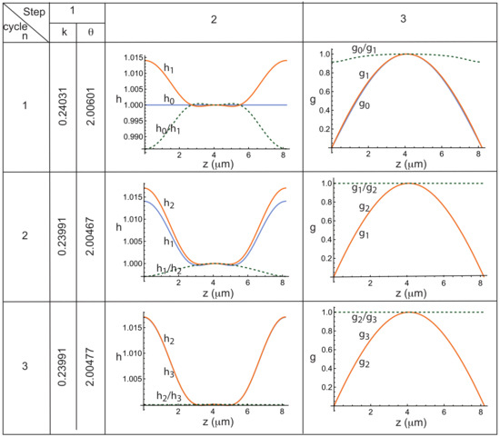
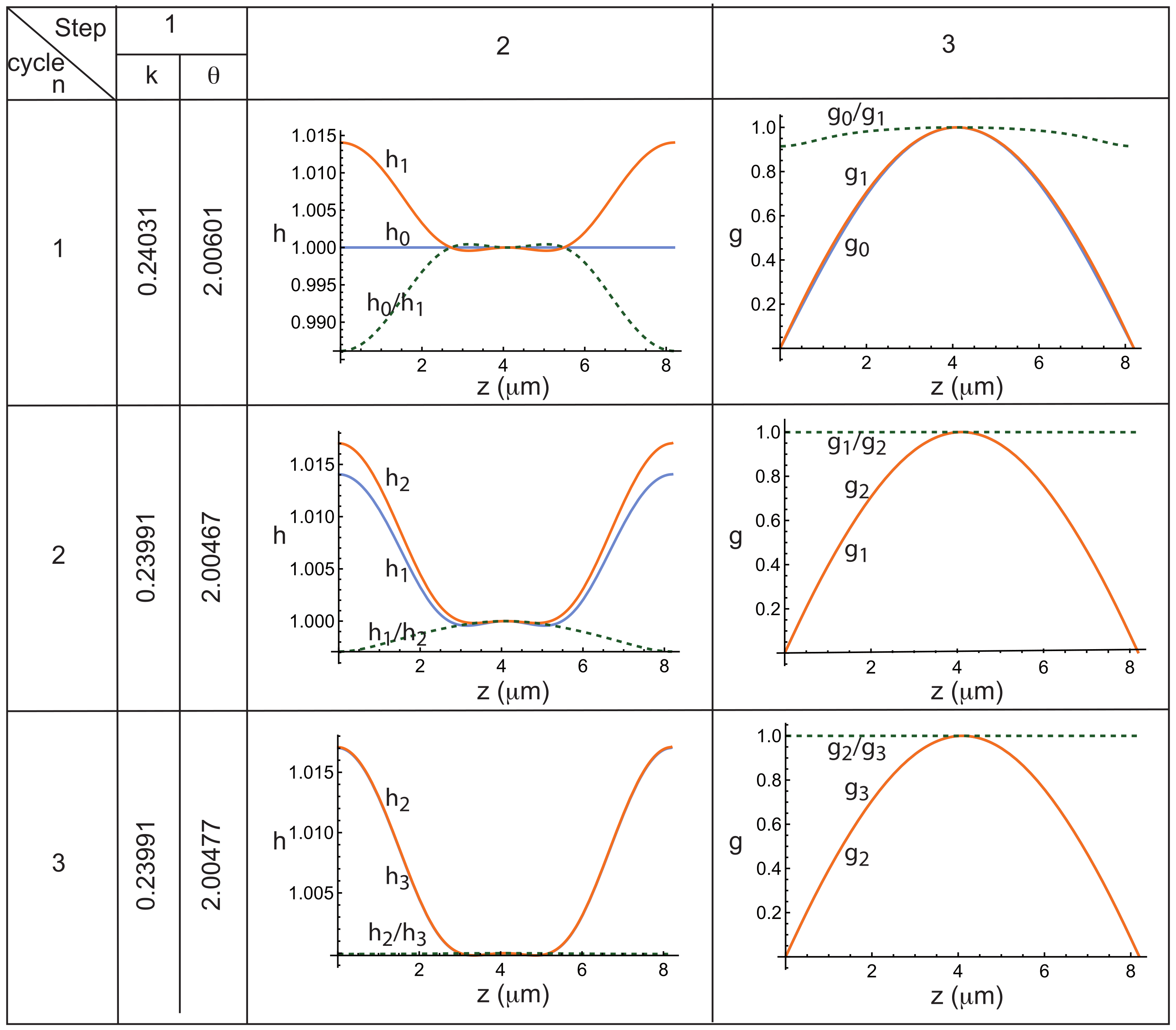
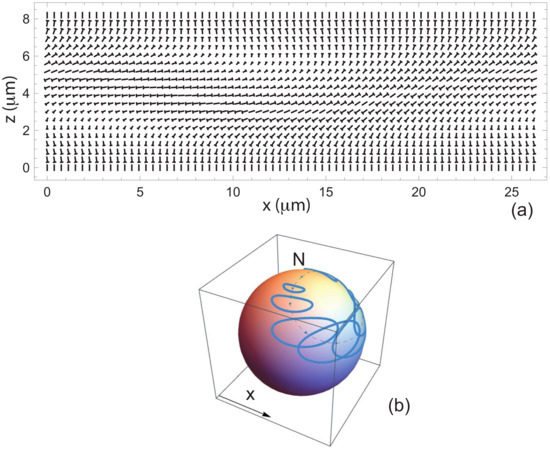
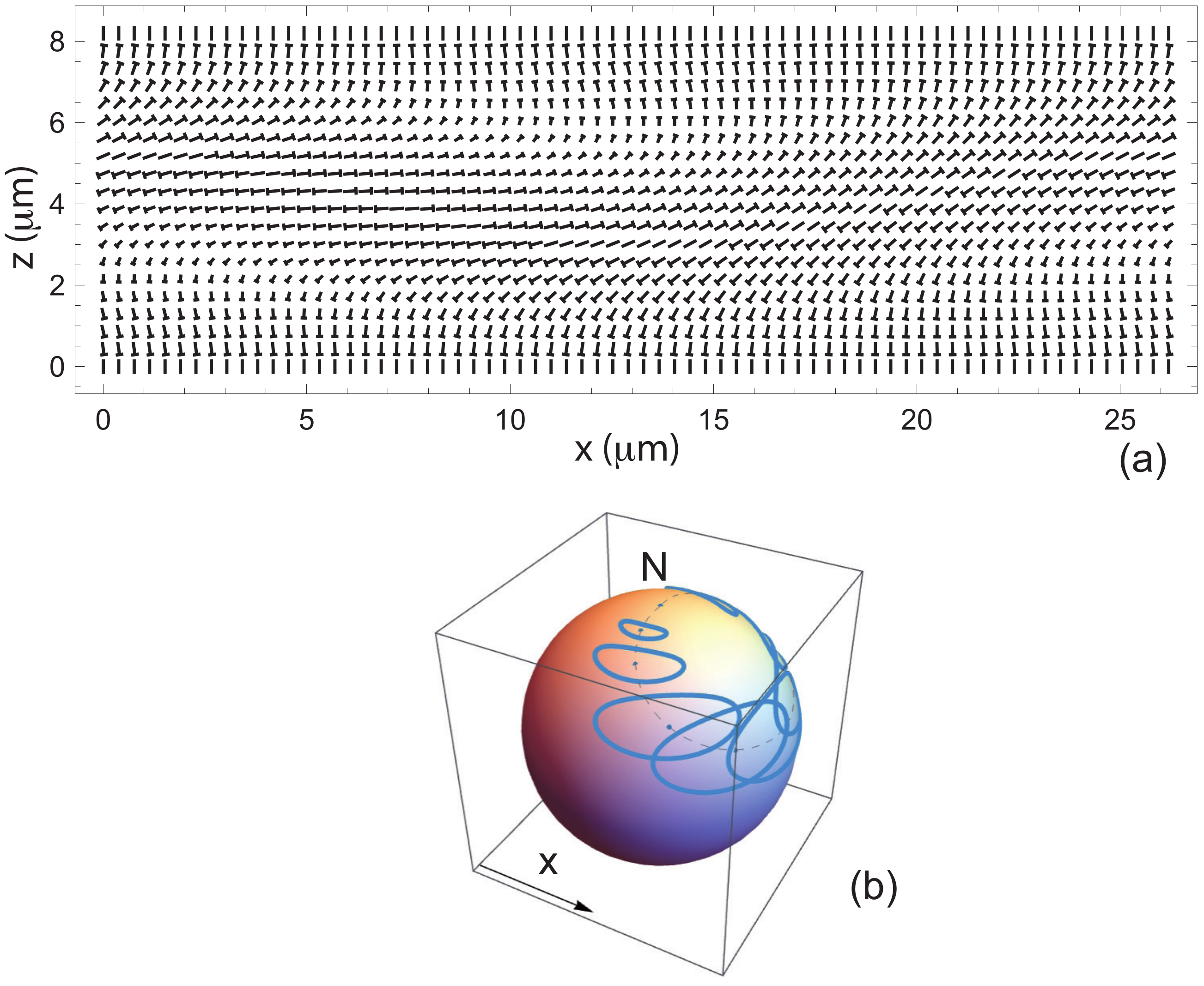
As an example, we investigated whether the TIC shown in Figure 1—calculated using , and T—is stable. The calculation reveals that it is unstable () for a wave vector m−1, corresponding to a wavelength m, and an angle rad. To illustrate the calculation of the wave vector k, the angle and the functions h and g, we have reproduced in Figure 2 how these quantities evolve at each step of the computation. In particular, in each graph, three curves are plotted: the function h or g computed at cycle (blue curve, denoted or ), the function h or g calculated at cycle n (orange curve, denoted or ), and the ratio between these two functions (green dashed curve, or ) which must tend to 1 if the process converge. This figure clearly shows that, in this example, the convergence is very rapid, with the functions and , as well as and , becoming indistinguishable as early as cycle . It is also worth noting here that the functions f and g differ only slightly from the initial functions and , which is not always the case, as will be seen in Section 4. The table also shows that the computed values of k and remain unchanged within an accuracy of from cycle onward. We also calculated the angle , which in this case is 0.277 rad. The corresponding director field is shown in Figure 3a in a plane perpendicular to the finger. The trajectories of the director on the sphere , when moving along straight lines perpendicular to the finger at , , , …, , are displayed in Figure 3b. These trajectories are not circular, as assumed in our previous work (Ref. [15]), but instead form flattened ellipses.
Figure 2.
Evolution of the functions h and g, as well as of the quantities k (in ) and (in rad), over the three steps of each computation cycle for –3. Calculations performed for the mixture MLC2079/R811 using m, , T, and the material constants given in Table 1.
Figure 3.
(a) Director field in the plane perpendicular to the periodic fingers. (b) Trajectories of the director on the sphere when moving along straight lines with equations , , , …, . The North pole represents the homeotropic nematic state. The dashed line represents the trajectory of the director in the TIC before destabilization. Calculations performed using m, , T, and the material constants of the mixture MLC2079/R811 given in Table 1.
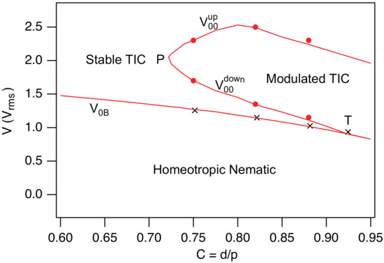
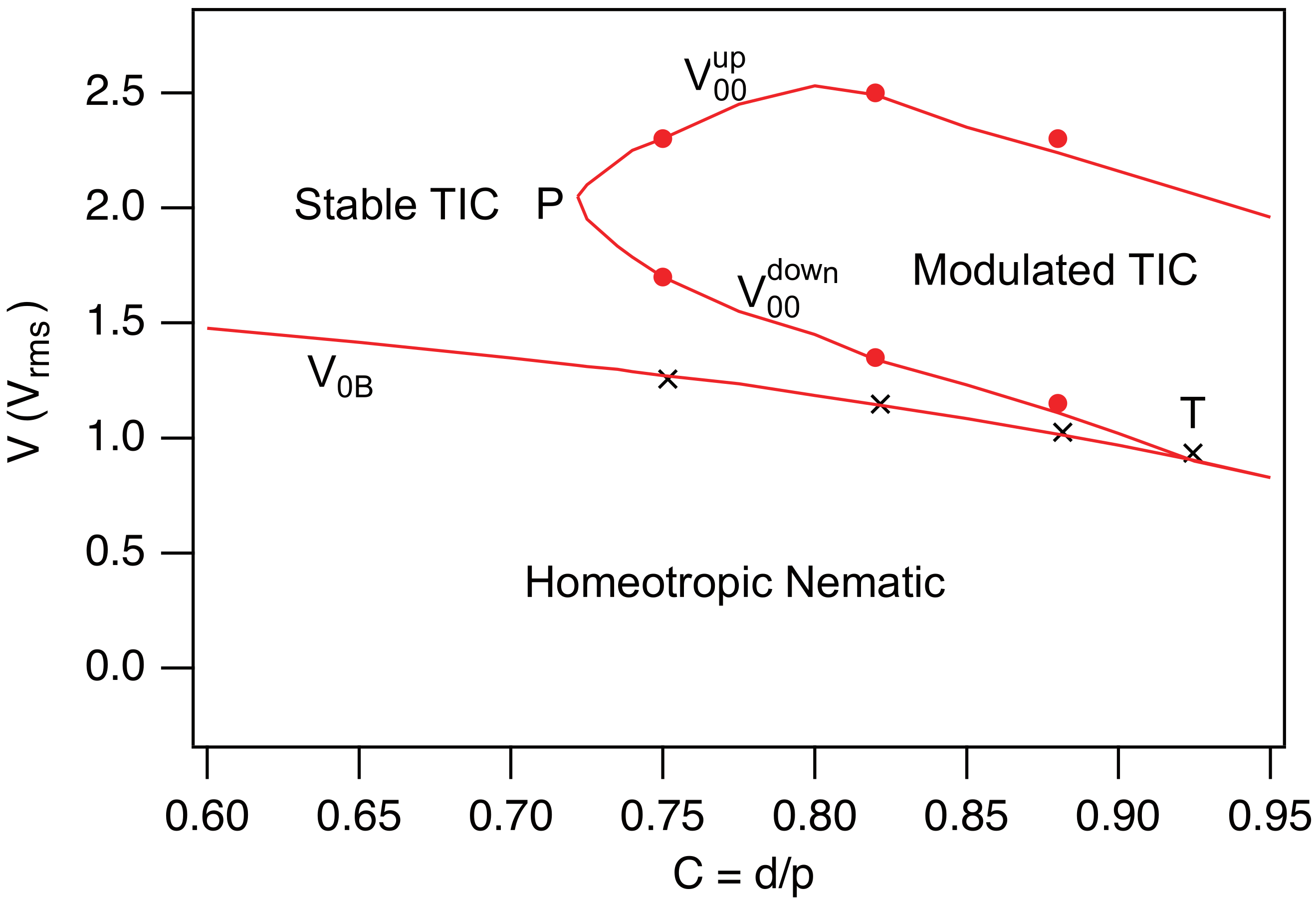
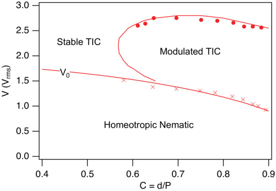
The same calculations can be performed for any values of the confinement ratio C and the applied voltage V, allowing us to determine at each point in the phase diagram whether the TIC is stable or unstable. In this way, we were able to identify the region of the phase diagram where the TIC destabilizes and develops fingers. Numerical calculations show that this region is bounded by two curves, and , located above the homeotropic nematic spinodal line given by Equation (12). These two curves meet at point P with coordinates and . It is worth noting that the curve intersects the nematic spinodal line at point T with coordinates and . Point T is a triple point, as the TIC, the modulated TIC (or periodic fingers), and the homeotropic nematic phase coexist at this point.
A particularly interesting observation is that between points P and T, we observe a re-entrance of the stable TIC: as the voltage is increased, the system successively transitions from the homeotropic nematic phase to a stable TIC, then to a modulated TIC, and finally back to a stable TIC at high voltage. We had already reported this re-entrance in the MLC2079/R811 system in our previous article [16]. It turns out that this phenomenon is very general and present in many systems, as first demonstrated experimentally by Smalyukh et al. in 2005 [14]. The origin of this re-entrant behavior will be analyzed in Section 2.5. Before doing so, let us examine in greater detail how these numerical results compare with the experimental data.
2.4. Comparison with Experiments
To test the relevance of these calculations, we prepared three homeotropic samples of different thicknesses using the liquid crystal MLC2079 doped with 0.813 wt.% of R811. For this concentration, . The sample preparation procedure and the experimental setup are the same as those described in Ref. [16]. The corresponding values of C are for sample 1, for sample 2, and for sample 3. To facilitate the measurement of the modulation wavelength at the threshold, each sample was placed on a Halbach magnet array, which imposes a horizontal magnetic field of 0.56 T. In this configuration, the TIC spontaneously aligns parallel to the magnetic field and destabilizes (when unstable) with a wave vector that is also parallel to the field. All experiments were carried out at room temperature ( °C), maintained using an air-conditioning system. At this temperature, the material constants of the MLC2079 liquid crystal (which melts above 100 °C) are nearly temperature-independent.
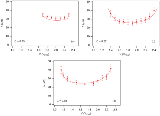
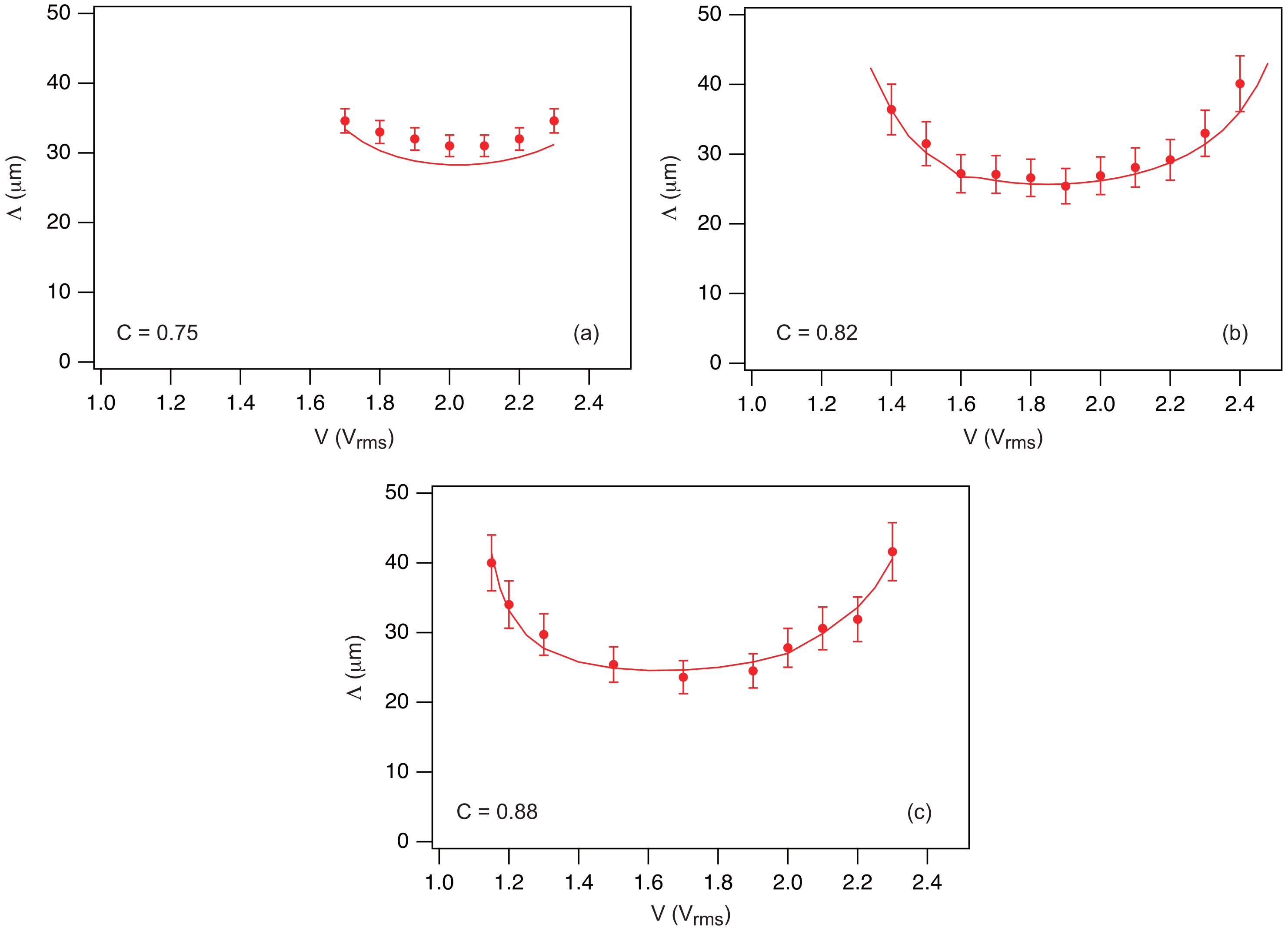
In practice, measurements of the TIC stability at a given voltage V were always performed starting from the homeotropic nematic phase. By doing this, the TIC develops rapidly (in less than a second) and then destabilizes slowly if it is unstable. In this way, we measured the voltage interval in which the TIC is effectively unstable. Our experimental data are plotted on the theoretical phase diagram shown in Figure 4 (solid circles). To complement these measurements, we measured (crosses in Figure 4) and, when the TIC was unstable, we additionally measured the modulation wavelength at the onset of instability. Our results are reported in Figure 5 for each sample (solid circles) and compared with numerical results (solid lines). As the reader can observe, the agreement is excellent for the phase diagram and remains very satisfactory for the wavelengths, which generally coincide within 10%.
Figure 4.
Theoretical phase diagram calculated for the mixture MLC2079/R811 when . A magnetic field of amplitude is applied along the x-axis. The dots and crosses are experimental points obtained with three samples of different thicknesses.
Figure 5.
Wavelength at the onset of instability as a function of the applied voltage measured in samples 1 (a), 2 (b) and 3 (c) (solid circles). The curves shown as solid lines were computed numerically by taking m and the material constants of the mixture MLC2079/R811 given in Table 1.
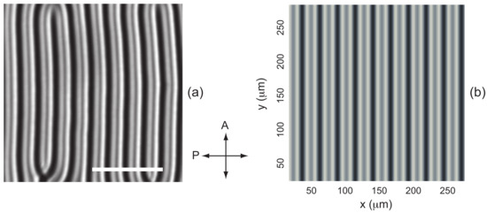
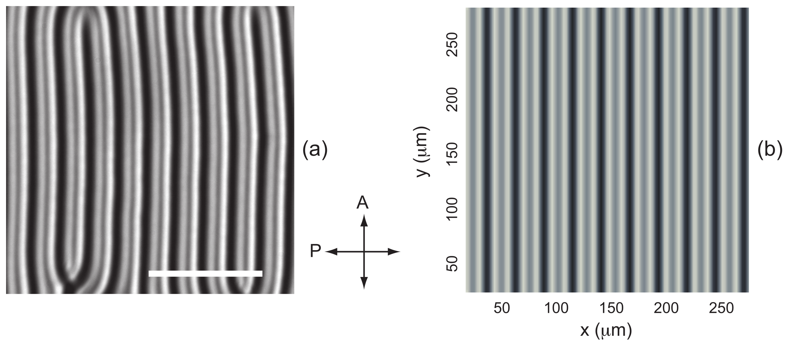
To complete this study, we examined whether images of the fingers calculated using the Jones formalism in the nonlinear regime are consistent with experimental observations. In the example shown in Figure 6, , , and , corresponding to the parameters already used to compute the director field in Figure 3. The calculated image closely resembles the experimental one, provided the upright microscope is focused on the upper surface of the sample. It should be noted that this is expected, since the Klein number of the finger pattern, defined as:
where is the wavelength of light and n the average refractive index, is about in this example, which is much smaller than unity. In this regime, it can be shown that there is no amplitude modulation in the exit plane of the sample (), the light being only phase-modulated [23]. This is precisely the basic assumption of the Jones formalism, which neglects diffraction. It is therefore not surprising that good agreement is observed only when focusing on the upper surface of the sample.
Figure 6.
(a) Fingers observed experimentally in sample 2 of the mixture MLC2079/R811 () at and . The photograph was taken between crossed polarizers in green light (). The white bar is long. The director field calculated for these parameters is shown in Figure 3a. (b) Image between crossed polarizers of these fingers calculated using the Jones formalism and the values of the indices given in Table 1.
Finally, we also calculated the phase diagram of the cholesteric mixture ZLI2806/S811 for , using the material constants listed in Table 2. The resulting phase diagram is shown in Figure 7. As in the previous case, a narrow range of the parameter C appears in which the stable TIC is re-entrant. Experimental data from Ref. [15] are also included and show excellent agreement with the theory. It should be noted that, in this experiment, the concentration of the chiral dopant S811 was 0.792 wt.%, corresponding to a pitch of .
Table 2.
Material constants of the Merck mixture ZLI2806 [24]. The elastic constants are given in pN.
Figure 7.
Phase diagram of the mixture ZLI2806/S811 when T. The solid lines have been calculated numerically with the constants given in Table 2. The solid circles and the crosses are taken from the experimental phase diagram given in Ref. [15].
2.5. Origin of the TIC Re-Entrance
As shown by the previous calculations, the emergence of a TIC modulation results from a subtle competition between several terms in the expression of the free energy of the system. These contributions can be calculated separately through the expression of the curvature term , which, after minimization, can be decomposed as follows:
In this formula, the first three terms describe the role of the elastic deformations associated with splay (), twist (), and bend (), while the fourth term () accounts for the effect of the electric field, and the fifth term () for the effect of the magnetic field. It is clear that the positive terms tend to stabilize the TIC, whereas the negative terms promote the onset of a modulation, and therefore the formation of fingers.
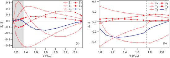
To understand the role of each of these terms, we calculated them separately as a function of the applied voltage for two different values of C, for which re-entrant TIC is either present or absent. The calculations were performed for the MLC2079/R811 mixture with (in this case, re-entrant TIC is observed) and with , for which the re-entrant behavior disappears. The two graphs of Figure 8 show that the splay term and the magnetic term are always positive, thereby stabilizing the TIC. The stabilizing effect of the magnetic field is clearly visible by comparing the phase diagrams in Figure 4 and Figure 11a (see below). In contrast, the twist term is always negative and promotes finger-like modulations. The remaining two terms depend strongly on the confinement ratio.
Figure 8.
Evolution as a function of the applied voltage V of the curvature term (evaluated after minimization, blue curve) and its different components () (red curves). In (a), and in (b), . In (a), the light gray shaded region corresponds to the TIC re-entrance domain, in which . It should be noted that in (a), the fingers are perpendicular to the magnetic field B. In (b), the fingers are perpendicular to B to the left of the vertical dashed line and parallel to B to the right. Calculations were performed for the MLC2079/R811 mixture using , , and the material constants listed in Table 1.
At low confinement (), the bend term is positive and exhibits a pronounced maximum at low voltage, whereas it becomes negative at high voltages, while the electric term is negative at low voltages and positive at high voltages (Figure 8a). In this regime, the re-entrant behavior of the TIC at low voltages is associated with the strong increase in , whereas at high voltages stabilization is driven by .
For , the electric term remains positive and thus stabilizes the TIC, particularly at high voltages, while the bend term is now always negative and favors finger-like modulations, even at low voltages (Figure 8b). For this reason the re-entrance disappears.
In conclusion, it appears quite clearly that the bend term is the one mainly driving the re-entrant behavior at low confinement ratios.
In the following, we show that these calculations can be easily extended to other geometries.
3. TIC Stability in Rubbed Homeotropic Samples
We have seen that a magnetic field can be used to orient the TIC [16]. Another method to orient it, first proposed by Smalyukh et al. in 2005 [14], consists of rubbing in a single direction the plates treated for homeotropic anchoring. This induces a slight tilt of the director at the plates in the rubbing direction, lifting the in-plane degeneracy and thus orienting the TIC. Another interesting result of Smalyukh et al. is that the TIC is more stable in rubbed samples than in purely homeotropic samples. We propose to demonstrate that these results can be reproduced numerically by adapting our calculations to the case of rubbed samples. In this context, two scenarios must be considered, as rubbing the plates in the same direction is not equivalent to rubbing them in opposite directions. We will refer to the former as ‘parallel rubbing’ and the latter as ‘antiparallel rubbing’.
3.1. Antiparallel Rubbing
In this case, Smalyukh et al. note that the TIC orients spontaneously in the rubbing direction [14]. To demonstrate this result, we must account for the fact that the anchoring is tilted by a small angle at the plates in the rubbing direction (which we choose to be parallel to the x-axis). In this case, the three bulk Equations (6)–(8) must be solved with new boundary conditions that depend on the anchoring conditions of the director at the plates.
Let denote the preferred anchoring direction on the plates. The surface energy can be written in the form [25]:
where is the anchoring energy. If is large (strong anchoring), the director will not deviate much from the direction on the plates. If, in addition, , can be expanded as a function of the angles , , and , which gives to second order in and :
In this form, it appears that the zenithal anchoring energy is much larger than the azimuthal anchoring energy, equal to . For this reason, the problem can be simplified by setting
on the two glass plates, which is a very good approximation in the strong anchoring regime, and by taking the azimuthal anchoring energy in the form:
knowing that when .
This results in the following boundary conditions for the angle :
where is the anchoring extrapolation length. Notice that the boundary conditions (11) remain unchanged for this configuration. Solving Equations (6)–(8) with the boundary conditions (32), (34), and (11) is straightforward using the Method of Lines in Mathematica.
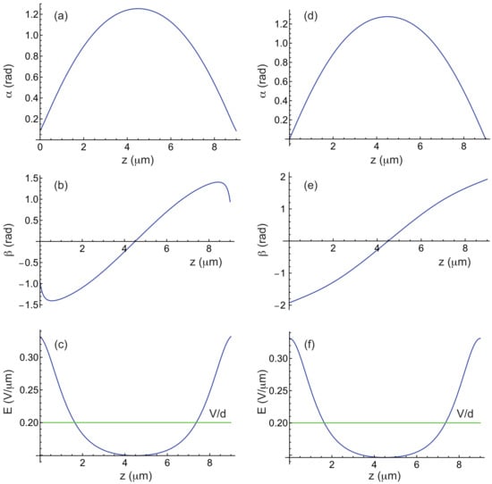
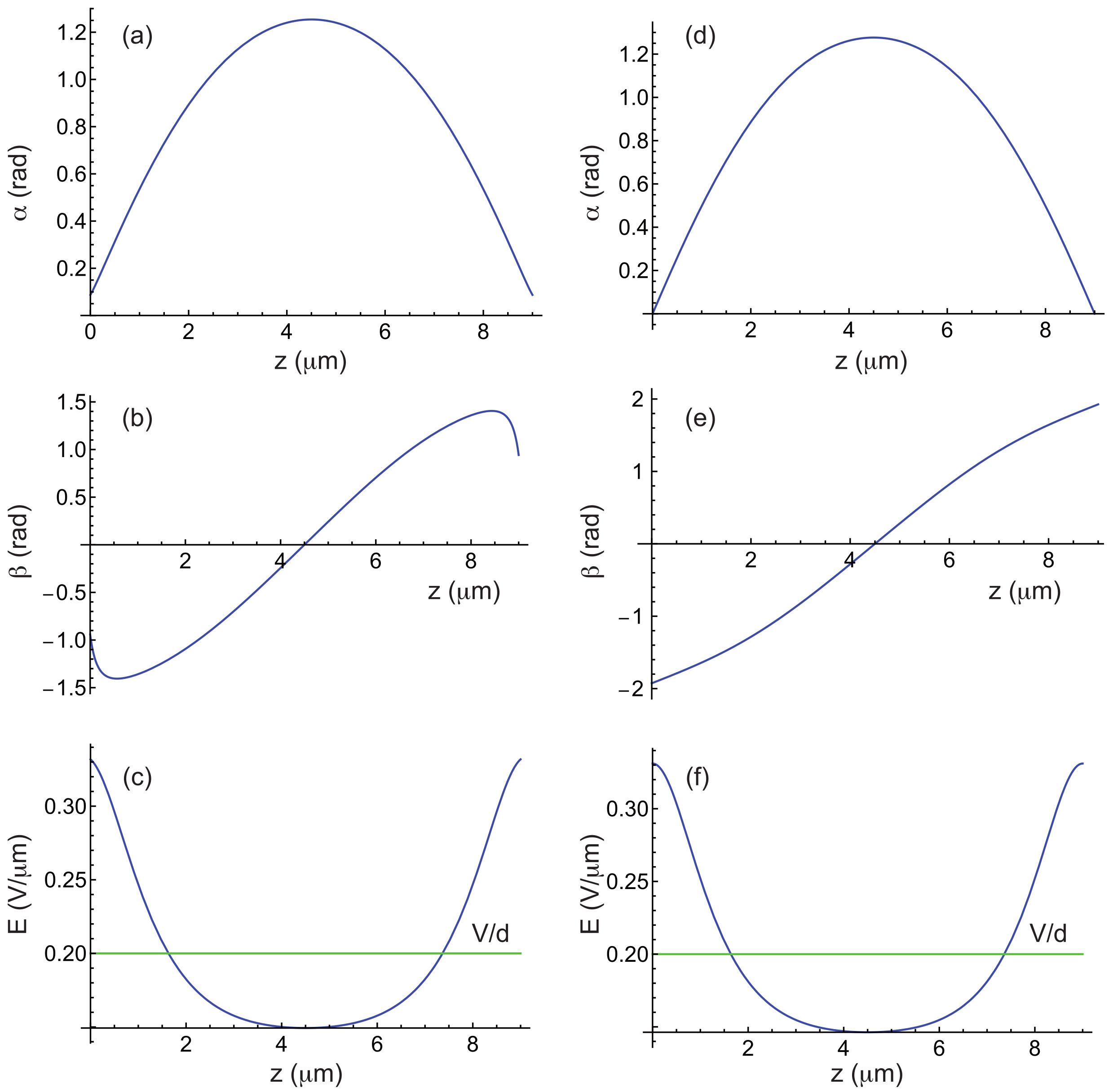
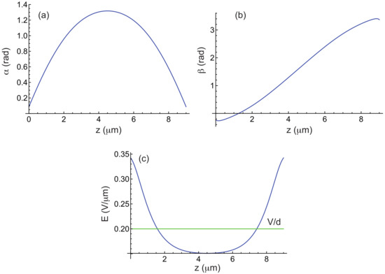
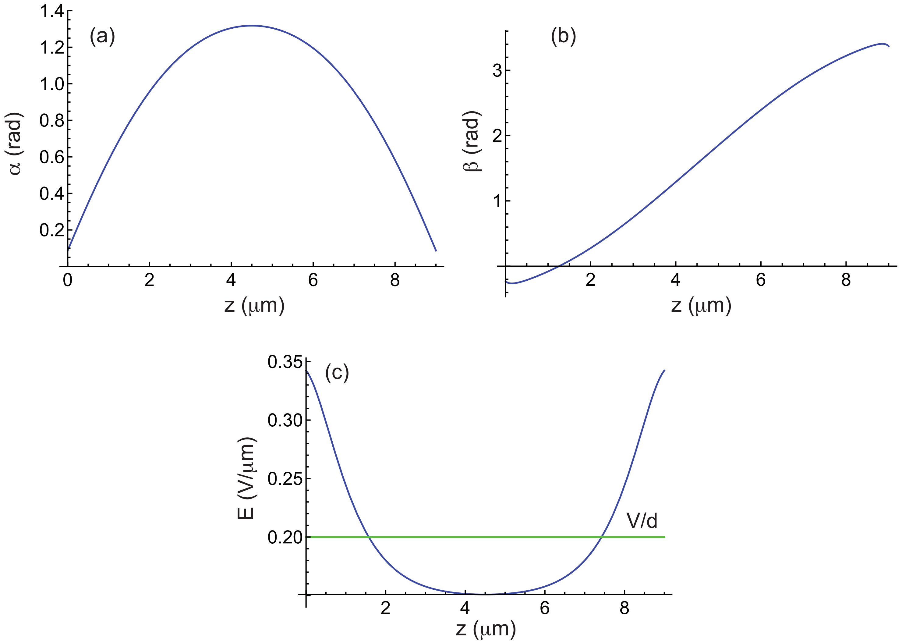
Figure 9 shows an example of calculated curves for the MLC2079/R811 mixture with , , and . The profile indicates that the TIC aligns along the rubbing direction, in agreement with experimental observations [14]. Comparison with Figure 1, obtained under similar conditions but with strong homeotropic anchoring, shows that the and profiles are nearly identical, the main difference arising in , which is strongly distorted near the plates due to rubbing.
Figure 9.
(a–c) Angles and and electric field E as a function of z in a TIC calculated by taking m, , , m, T, , and the material constants of the mixture MLC2079/R811 given in Table 1, when the two plates are rubbed in opposite directions. Curve (b) shows that , meaning that the -director is parallel to the rubbing direction (parallel to the x-axis). (d–f) The same curves plotted for comparison in the purely homeotropic case.
Now that the TIC is characterized, let us analyze its stability. For this calculation, the same ansatz for the director field as before can be used, given by Equation (14). The procedure remains largely the same, except that we must now account for new boundary conditions for the function h, which now read:
As for g, the boundary conditions (15) remain unchanged.
The other change concerns the energy per unit surface area, which now includes an anchoring energy term. After averaging along the x-direction, this term takes the form , taking into account that there are two surfaces and the symmetry condition . As a consequence, the curvature to minimize now reads in the form:
The minimization procedure is then exactly the same as in the purely homeotropic case. The calculations are only slightly longer due to the new boundary conditions that must be satisfied for the functions and .
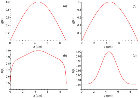
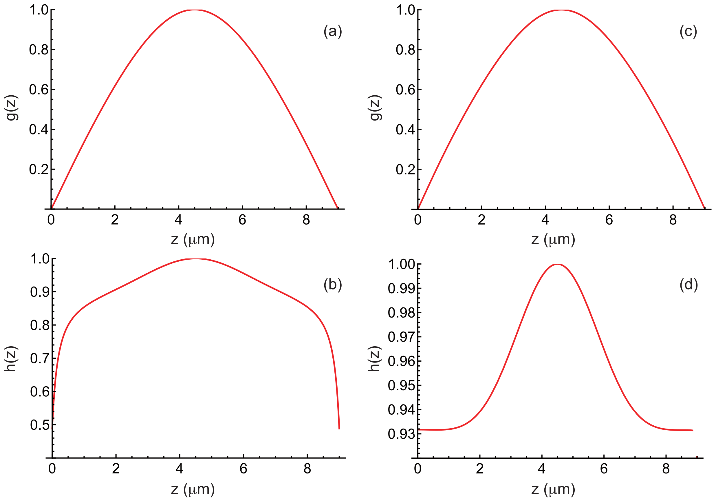
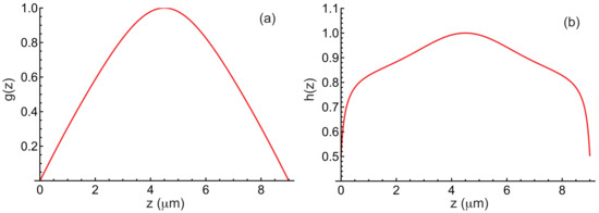
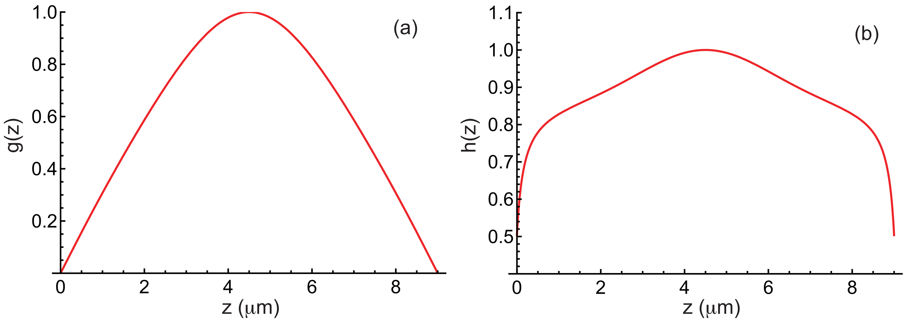
In Figure 10, we show the functions g and h obtained after convergence for , , , , , and by taking the material constants given in Table 1. As before, these functions are normalized by setting and . For comparison, the same functions are also shown in this figure for the purely homeotropic anchoring case. As expected, it is primarily the function h that changes in the presence of rubbing. We can also compare the values of k and obtained in both cases through minimization. In the case with rubbing, (corresponding to ) and , whereas in the purely homeotropic case, (corresponding to ) and . It thus appears that the modulation wavelength is slightly shorter in the rubbed case than in the purely homeotropic case.
Figure 10.
(a,b) Functions and calculated by taking , , , , , and the material constants of the mixture MLC2079/R811 given in Table 1, when the plates are rubbed in opposite directions. (c,d) The same curves plotted for comparison in the purely homeotropic case.
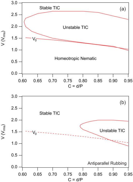
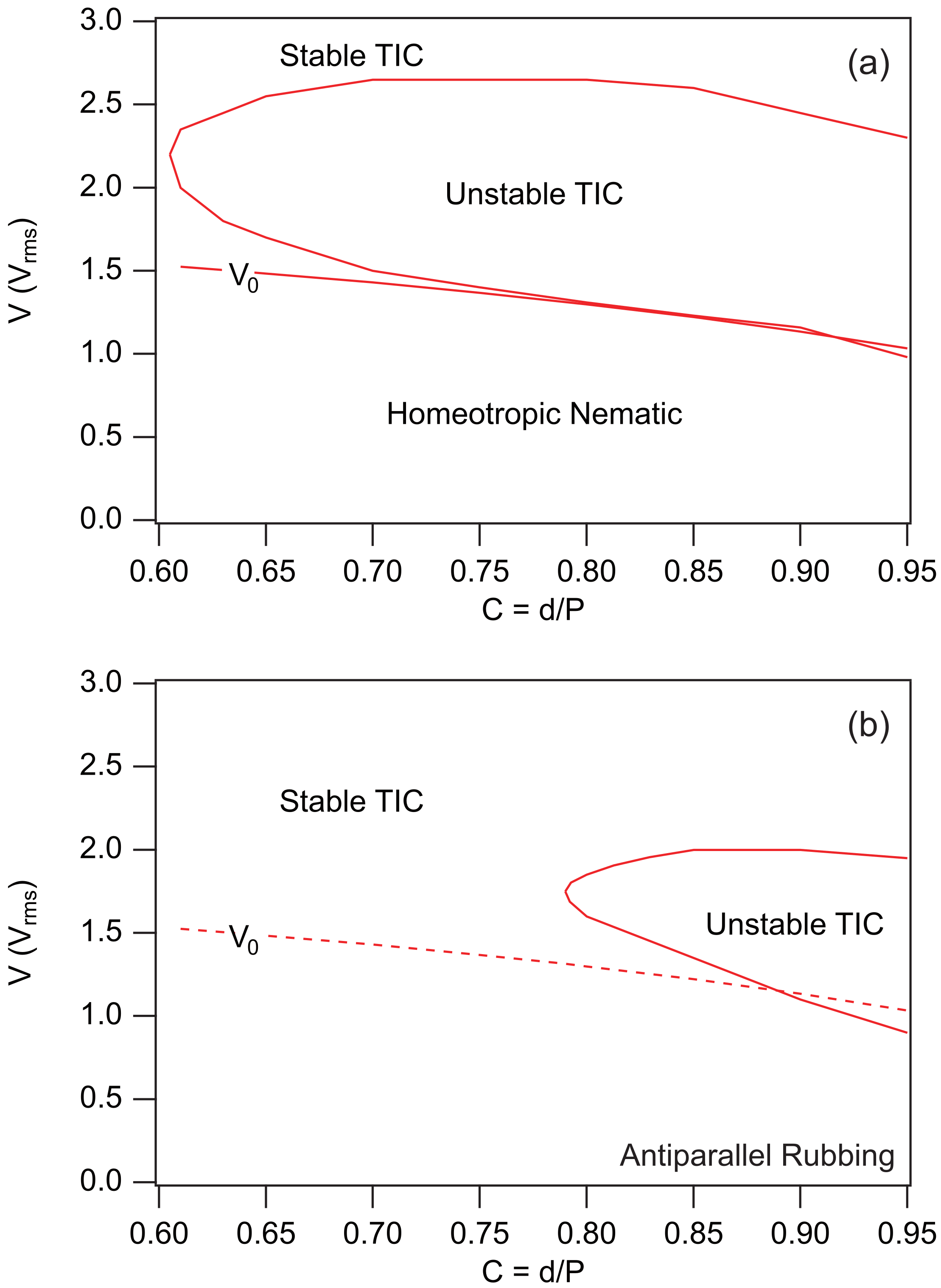
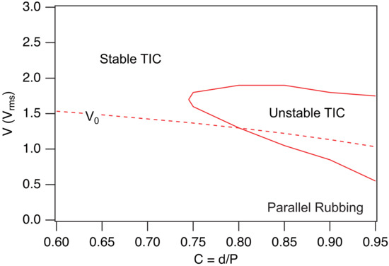
To delve deeper into the comparison, we recalculated the phase diagrams for the MLC2079/R811 mixture when and in both the purely homeotropic case and the rubbed case when the plates are rubbed in opposite directions, still using and . These two diagrams are reported in Figure 11. It clearly appears that rubbing the plates extends the stability region of the TIC. This result is in close agreement with the observations of Smalyukh et al. [14]. It is also worth noting, by comparing the diagrams in Figure 4 and Figure 11a, that applying a magnetic field also stabilizes the TIC.
Figure 11.
Phase diagrams calculated when T in the MLC2079/R811 mixture with . (a) Homeotropic anchoring. (b) Rubbed homeotropic anchoring with and when the two plates are rubbed in opposite directions. In this case, there is no longer homeotropic nematic phase since the anchoring is tilted on the plates. This is why we plotted the line as a dashed curve. This line nevertheless marks the boundary between a low-amplitude TIC and a fully developed TIC.
We now analyze the case of parallel rubbing.
3.2. Parallel Rubbing
In this case, the boundary conditions for the angle remain unchanged, given by Equation (32). However, the anchoring energy must now be expressed in two different forms on the two plates, namely:
With this choice, the boundary conditions for the angle become:
As for the bulk equations, they remain unchanged. Solving the new equations is again straightforward with Mathematica. Figure 12 shows an example of calculated curves for the MLC2079/R811 mixture with , , and . The profile indicates that the TIC aligns now perpendicular to the rubbing direction, as . Again, the and profiles are nearly identical to those calculated under homeotropic anchoring. On the other hand, the profile is different—centered around and much less deformed near the plates than in the case of antiparallel rubbing.
Figure 12.
Angles (a) and (b) and electric field E (c) as a function of z in a TIC calculated by taking m, , , m, T, , as well as the material constants of the mixture MLC2079/R811 given in Table 1, when the two plates are rubbed in the same direction. Curve (b) shows that , meaning that the -director orients now perpendicular to the rubbing direction (parallel to the x-axis).
The next step is to calculate the stability of the TIC. The calculation is carried out exactly as before. The expression for remains unchanged and given by Equation (36), and the boundary conditions for g and h are still provided by Equations (15) and (35), respectively. In Figure 13, we show the functions g and h obtained after convergence for , , , , , and . As before, these functions are normalized by setting and .
Figure 13.
Functions (a) and (b) calculated by taking , , , , , and the material constants of the mixture MLC2079/R811 given in Table 1, when the plates are rubbed in the same direction.
Again, the function closely resembles that calculated for homeotropic anchoring, but the function is quite different, as can be seen by comparing with the curves shown in Figure 10c,d. In this example, the calculation yields (corresponding to a wavelength ) and . Once again, the wavelength is very similar to that calculated for a homeotropic sample.
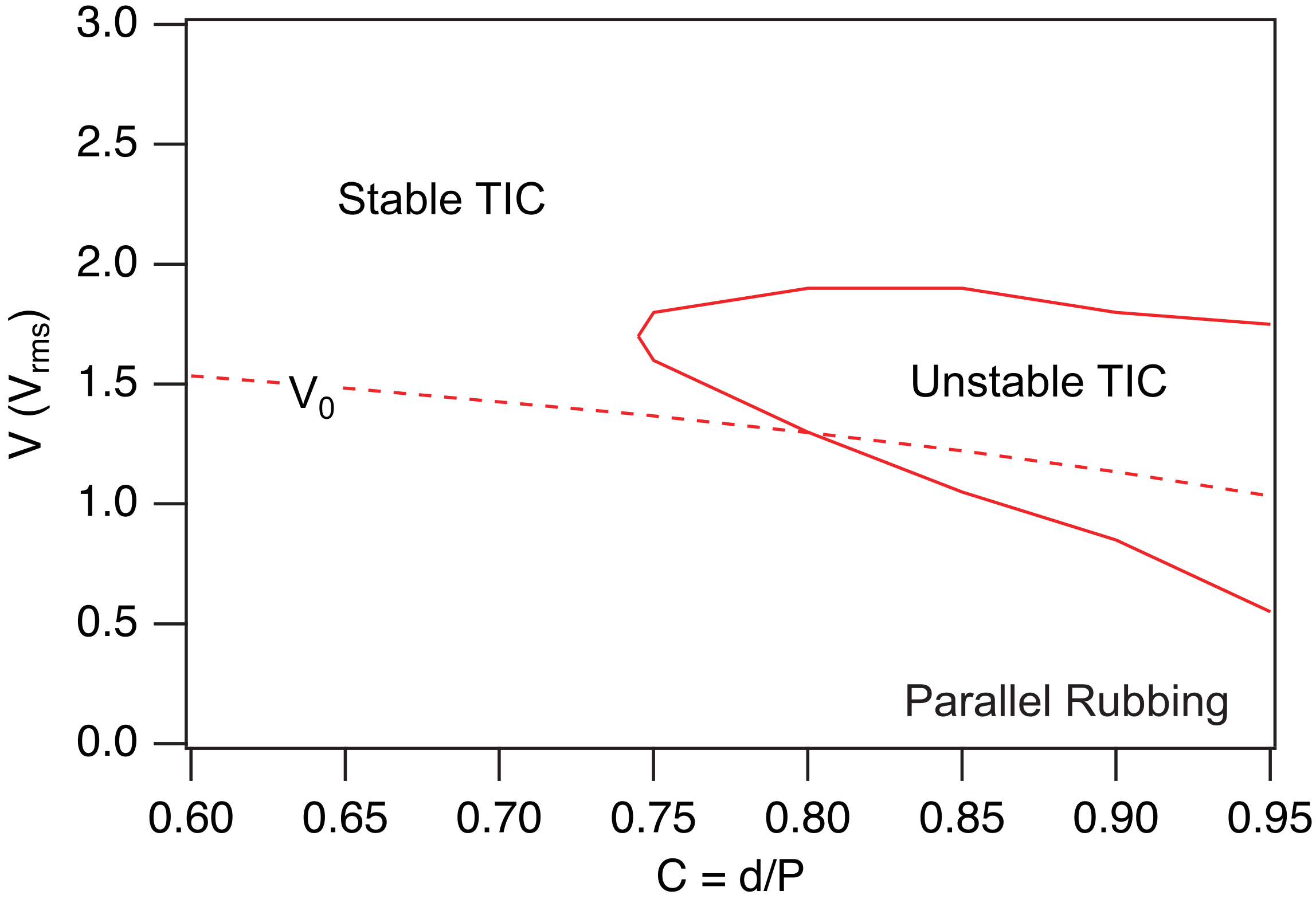
Finally, we recalculated the phase diagram of the MLC2079/R811 mixture for when the plates are rubbed in the same direction, using , , and . The result is shown in Figure 14. Comparison with Figure 11 indicates that rubbing the plates in the same direction extends the stability region of the TIC, albeit less than in the case of oppositely rubbed plates.
Figure 14.
Phase diagram of the MLC2079/R811 mixture calculated when the two plates are rubbed in the same direction and T, , , and . The material constants are given in Table 1.
4. TIC Stability in Hybrid Samples
A TIC can also develop in a cholesteric sample confined between a plate treated for strong unidirectional planar anchoring and a plate treated for strong homeotropic anchoring. Experiments show that this TIC is stable in thin samples (typically when ) and develops a striped texture at larger thicknesses [26,27,28,29]. This instability leads, in particular, to a typical arch-like texture in a wedge-shaped sample, with the modulation wave vector rotating by each time the thickness increases by an amount equal to the cholesteric pitch. Note that the same instability has also recently been observed in thin layers of cholesteric liquid crystal deposited by spin coating onto a substrate with unidirectional planar anchoring, when the air interface exhibits homeotropic anchoring [30].
To analyze this texture, we used in Ref. [26] a simplified model for the TIC and the ’circle model’ on the sphere to study its stability. Although this model was highly qualitative, it allowed us to predict the existence of a striped instability and to reproduce qualitatively the arch-like texture in a wedge sample. However, it did not allow us to demonstrate the existence of a critical thickness below which the TIC is stable, nor to correctly predict the wavelength of the stripes and their orientation relative to the planar anchoring direction.
In this section, we show that with the new procedure described in this article we can recover the main experimental results reported in Ref. [26]. In this work, the cholesteric material used was 8CB-doped with 2.19 wt% of the chiral mesogen CB15. All measurements were performed at 38 °C, for which the cholesteric pitch is .
In the following, we assume that the modulation wave vector is oriented along the x-axis and that the planar anchoring direction on the bottom plate makes an angle with the x-axis. As for the top plate, it is treated for homeotropic anchoring. No external fields are applied to the sample ( and ). We must then solve the two TIC Equations (6) and (7) with the following boundary conditions:
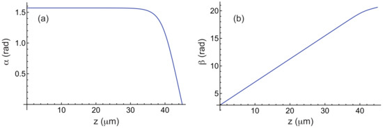
which is again straightforward in Mathematica by using the Method of Lines. Figure 15 shows the functions and calculated numerically for and , using the elastic constants of 8CB given in Table 3, which is the liquid crystal used in Ref. [26].
Figure 15.
Angles (a) and (b) as a function of z in a TIC calculated by taking , , and the material constants of 8CB given in Table 3. The bottom plate is treated for planar unidirectional anchoring along the direction and the top plate is treated for homeotropic anchoring.
Table 3.
Material constants of 8CB at T = 38 °C. The elastic constants are given in pN [31] and the indices have been measured at nm [32].
To analyze the stability of this solution, we use again the ansatz given in Equation (14). In this case, the function g must satisfy the boundary conditions (15) and the function h:
The procedure for minimizing the curvature is essentially the same as before, except that this quantity must now be minimized with respect to as well. In practice, we fix the angle , compute the TIC, and then minimize (given by Equation (20)) with respect to the parameters k and , as well as the functions g and h. To perform this minimization, we use the following functions as initial guesses for g and h:
These functions satisfy the boundary conditions (15) and (41). Note that, in this calculation, the functions g and h are normalized such that and .
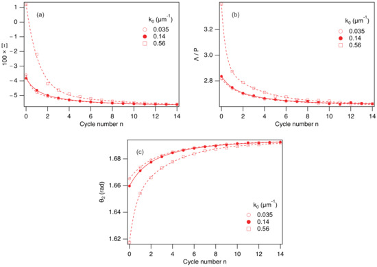
In practice, the minimization procedure must be adapted because the chosen functions and are far from the final solutions. In particular, minimizing with respect to k and (for a given angle ) by taking the functions and most often leads to , which prevents further calculation. To bypass this difficulty, the minimization is initially performed by fixing k to a non-zero starting value (for example, ). The function is then minimized with respect to , yielding a value . We then calculate the function g that minimizes by setting , , and . This gives . With this function and by taking , we then minimize with respect to k and , resulting in and . Using these values, we subsequently minimize with respect to h by setting , yielding . Finally, we minimize with respect to k and , which gives and . These calculations can then be repeated several times until the process reaches final convergence. In practice, 10 to 15 cycles are required for convergence, which typically takes between 30 s and 1 min, a reasonable time frame.
The convergence process is illustrated in Figure 16, where we show how the quantities , , and converge as a function of the cycle number n when and . This figure also shows that these quantities converge toward the same solution, regardless of the chosen value of the initial wave vector , indicating that the solution is unique.
Figure 16.
Three graphs showing the convergence of the quantities (a), (with ) (b), and (c) in the mixture 8CB/CB15 as a function of the cycle number n for three different values of the initial wave vector . The solid and dashed curves correspond to double-exponential fits of the numerical data. and .
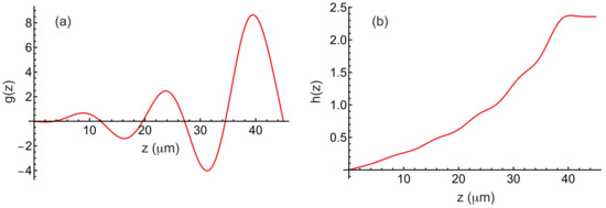
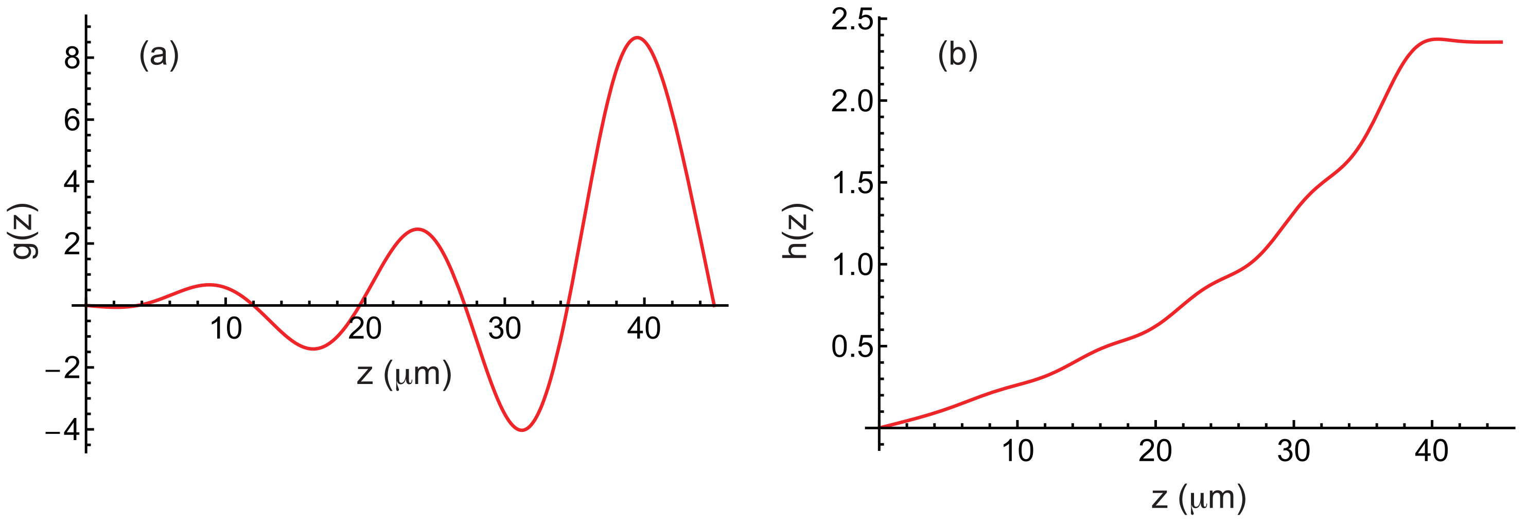
The functions f and g obtained after convergence are also shown in Figure 17. The calculation shows that is minimal for , (corresponding to a wavelength ) and .
Figure 17.
Function g (a) and h (b) in a hybrid sample plotted as a function of z when , and (for this value, is minimal). The material constants of 8CB are given in Table 3. The bottom plate is treated for planar unidirectional anchoring along the direction and the top plate is treated for homeotropic anchoring.
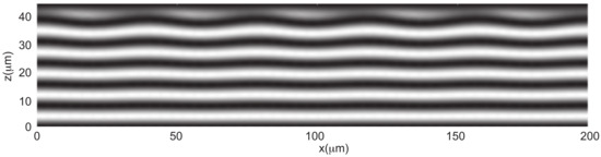
To go further, we also calculated the angle that minimizes the energy F, while using the functions f and g calculated at the onset of instability and setting . This calculation yields and . These angles are very small, indicating that the modulation is of low amplitude. In Figure 18, we show the density plot of the component in a plane perpendicular to the stripes. This representation reveals that the layers undulate and that this undulation propagates throughout the sample thickness, starting from the top plate treated for homeotropic anchoring.
Figure 18.
Density plot of in the plane perpendicular to the stripes. Five wavelengths are represented. This plot reveals the undulation of the cholesteric layers of thickness .
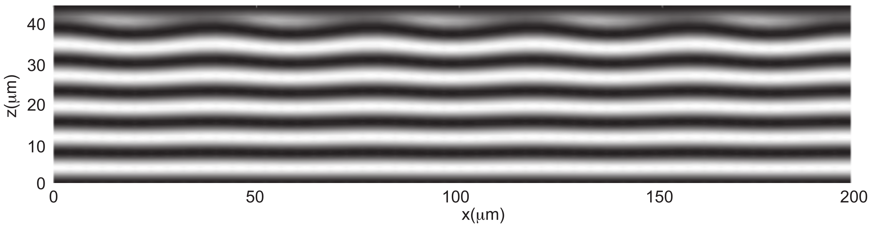
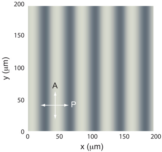
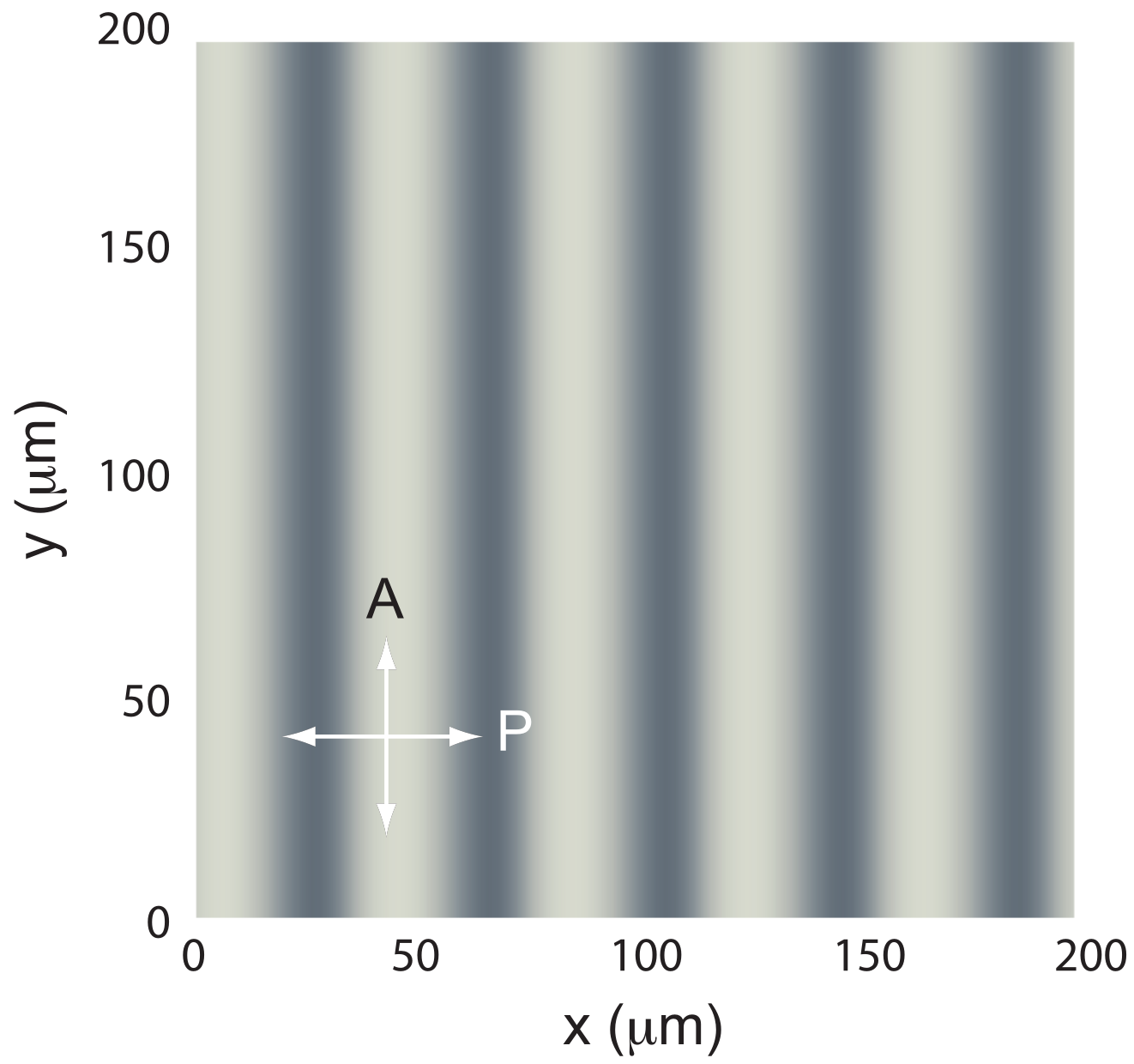
We also calculated the image of the sample when observed between crossed polarizers (Figure 19). The calculation using Jones matrices shows that the stripes must be perfectly visible under a polarizing microscope, in agreement with experiments.
Figure 19.
Image of the stripes between crossed polarizers, calculated using Jones matrices.
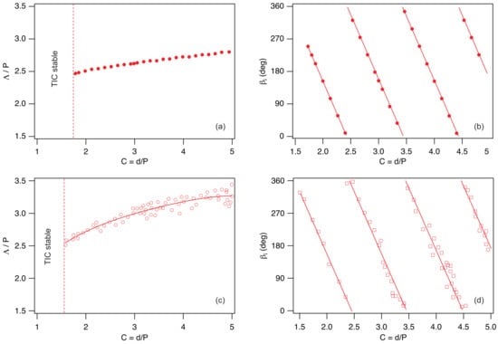
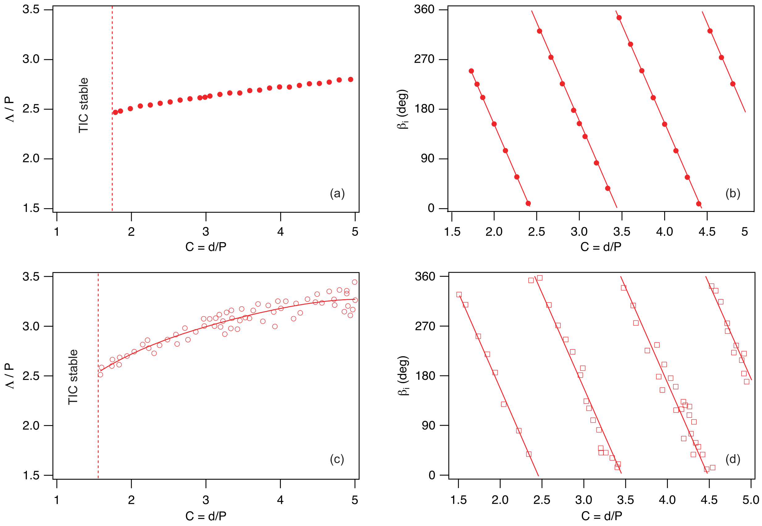
The same calculations can be repeated for each thickness. They show that there exists a critical thickness below which the TIC is stable. In our case, this thickness is , corresponding to a confinement ratio . This value is in reasonably good agreement with the experimental one: . We can also calculate, for each thickness , the modulation wavelength and the angle that the wave vector makes with the rubbing direction. These results are shown in Figure 20a,b, and are again in fairly good agreement with the experimental results shown just below in Figure 20c,d. The new model therefore represents a significant improvement over our previous one [26], which, for instance, failed to predict the existence of a critical thickness below which the TIC is stable. It also provides much better agreement for the wavelengths, correctly capturing their increase with the confinement ratio, in contrast to the previous one, which underestimated the wavelengths and predicted a decrease with increasing confinement ratio.
Figure 20.
Stripe wavelength (a) and angle (b) between the wave vector and the rubbing direction calculated numerically as a function of the confinement ratio by taking the material constants of 8CB given in Table 3. (c,d) Corresponding experimental data for the mixture 8CB/CB15 at 38 °C from Ref. [26].
5. Conclusions
In conclusion, we have developed in this article a new method that allows one to study the stability of a TIC in a cholesteric sample confined between two parallel plates. In this model, the TIC is computed numerically by directly solving the torque balance equations together with Maxwell’s equation for the electric field, so that no approximations are introduced at this stage. This solution is then destabilized using a new ansatz for the director field. This ansatz is more general, yet paradoxically simpler, than the one used in our previous work [20], which was based on the ‘circle model’ on the sphere .
Using this model, we first showed that it is possible to reconstruct, in a very short computation time, the phase diagram of a homeotropic cholesteric sample with negative dielectric anisotropy. One of the main strengths of this model is that it captures the re-entrance of the stable TIC observed experimentally at low confinement ratios [14]. Another important feature is its ability to predict with good accuracy the wavelength of the fingers in the unstable regime, which may be relevant for applications.
We then generalized the model to other geometries. In particular, we showed how the phase diagram of a homeotropic cholesteric sample with negative dielectric anisotropy is modified when the plates are rubbed in a given direction. In this way, we demonstrated that the TIC aligns parallel to the rubbing direction for parallel rubbing, whereas it aligns perpendicular to it for antiparallel rubbing. We also found that rubbing tends to stabilize the TIC, in agreement with the experimental observations of Smalyukh et al. [14].
Finally, we revisited the problem of TIC stability in hybrid cells. We confirmed the existence of a critical thickness below which the TIC is stable, a feature that could not be predicted by our previous model [26]. The predicted wavelengths are also in much better agreement with experiments. Moreover, this model reveals that the stripe instability is coupled to an undulation of the layers across the sample thickness, a feature that had not been anticipated in our earlier work.
One of the main limitations of our model is that it implicitly assumes a unidirectional modulation of the TIC. In practice, this is indeed the case in homeotropic samples at low confinement ratios, where the modulation wave vector is always perpendicular to the TIC. The situation becomes more complex as the confinement ratio increases, since experiments show that a two-dimensional modulation, most often square, develops at the instability threshold. This instability was clearly observed under directional growth conditions when the cholesteric phase was grown sufficiently rapidly from the homeotropic nematic phase near the smectic A phase in the presence of a temperature gradient [33].
It would therefore be of interest to extend the present model to the two-dimensional case. Nevertheless, the present model can still be applied at large thicknesses when fingers reappear, as already mentioned in our previous work [16]. In this regime, the fingers are parallel to the TIC, a case that will be addressed in a forthcoming article.
Funding
This research received no external funding.
Data Availability Statement
Data and numerical tools are available from corresponding author upon reasonable request.
Acknowledgments
I would like to warmly thank G. Poy and J. Ignés Mullol for their careful proofreading of the manuscript, and G. Poy for his very insightful remarks on anchoring energy and the Klein number. The author used ChatGPT (OpenAI), based on the GPT-5.5 model, solely for minor English language editing (wording and expression checks). No scientific content, analysis, or interpretation was generated by AI.
Conflicts of Interest
The author declares no conflicts of interest.
Appendix A. Functions
Appendix B. Rules for Calculating the Functions a1, a2, …
Appendix C. Rules for Calculating the Functions , , …
References
- de Gennes, P.G.; Prost, J. The Physics of Liquid Crystals; Clarendon Press: Oxford, UK, 1993. [Google Scholar]
- Oswald, P.; Pieranski, P. Nematic and Cholesteric Liquid Crystals: Concepts and Physical Properties Illustrated by Experiments; The Liquid Crystals Book Series; Taylor & Francis: Boca Raton, FL, USA, 2005; 618p. [Google Scholar]
- Belyakov, V.A.; Dmitrienko, V.E.; Orlov, V.P. Optics of cholesteric liquid crystals. Sov. Phys. Usp. 2013, 22, 64–88. [Google Scholar] [CrossRef] [Scilit]
- Ma, J.; Xuan, L. Towards nanoscale molecular switch-based liquid crystal displays. Displays 2013, 34, 293–300. [Google Scholar] [CrossRef] [Scilit]
- Coates, D. Development and applications of cholesteric liquid crystals. Liq. Cryst. 2015, 42, 653–665. [Google Scholar] [CrossRef] [Scilit]
- Balamurugan, R.; Liu, J.H. A review of the fabrication of photonic band gap materials based on cholesteric liquid crystals. React. Func. Pol. 2016, 105, 9–34. [Google Scholar] [CrossRef] [Scilit]
- Zhou, H.; Wang, H.; He, W.; Yang, Z.; Cao, H.; Wang, D.; Li, Y. Research Progress of Cholesteric Liquid Crystals with Broadband Reflection. Molecules 2022, 27, 4427. [Google Scholar] [CrossRef] [Scilit]
- Dowden, W.A. Cholesteric liquid crystals: A review of developments and applications. Non-Destr. Test. 1967, 1, 99–102. [Google Scholar] [CrossRef] [Scilit]
- Chen, J.; Feng, X.; Huang, J.; Li, X.; Huang, S.; Wu, Z.; Qiu, L.; Cao, L.; Liang, Q.; Li, X. Microfluidics-Assisted Three-Dimensional Confinement of Cholesteric Liquid Crystals for Sensing Applications. Micromachines 2026, 17, 244. [Google Scholar] [CrossRef] [Scilit]
- Cladis, P.E.; Kleman, M. The cholesteric domain texture. Mol. Cryst. Liq. Cryst. 1972, 16, 1–20. [Google Scholar] [CrossRef] [Scilit]
- Press, M.J.; Arrott, A.S. Static strain waves in cholesteric liquid crystals.-I. homeotropic boundary conditions. J. Phys. Paris 1976, 37, 387–395. [Google Scholar] [CrossRef] [Scilit]
- Gil, L.; Gilli, J.M. Surprising dynamics of some cholesteric liquid crystal patterns. Phys. Rev. Lett. 1998, 80, 5742. [Google Scholar] [CrossRef] [Scilit]
- Oswald, P.; Baudry, J.; Pirkl, S. Static and dynamic properties of cholesteric fingers in electric field. Phys. Rep. 2000, 337, 67–96. [Google Scholar] [CrossRef] [Scilit]
- Smalyukh, I.I.; Senyuk, B.I.; Palffy-Muhoray, P.; Lavrentovich, O.D.; Huang, H.; Gartland, E.C.; Bodnar, V.H.; Kosa, T.; Taheri, B. Electric-field-induced nematic-cholesteric transition and three-dimensional director structures in homeotropic cells. Phys. Rev. E 2005, 72, 061707. [Google Scholar] [CrossRef] [Scilit] [PubMed]
- Ribière, P.; Pirkl, S.; Oswald, P. Electric-field-induced phase transitions in frustrated cholesteric liquid crystals of negative dielectric anisotropy. Phys. Rev. A 1991, 44, 8198–8209. [Google Scholar] [CrossRef] [Scilit]
- Oswald, P.; Poy, G.; Ignés-Mullol, J. TIC Reorientation under Electric and Magnetic Fields in Homeotropic Samples of Cholesteric LC with Negative Dielectric Anisotropy. Crystals 2023, 13, 957. [Google Scholar] [CrossRef] [Scilit]
- Smalyukh, I.I.; Lansac, Y.; Clark, N.A.; Trivedi, R.P. Three-dimensional structure and multistable optical switching of triple-twisted particle-like excitations in anisotropic fluids. Nat. Mater. 2010, 9, 139–145. [Google Scholar] [CrossRef] [Scilit]
- Wu, J.; Smalyukh, I.I. Hopfions, heliknotons, skyrmions, torons and both abelian and nonabelian vortices in chiral liquid crystals. Liq. Cryst. Rev. 2022, 10, 34–68. [Google Scholar] [CrossRef] [Scilit]
- Torres-Andrés, J.; Coelho, R.C.V.; Oswald, P.; Sagués, F.; Ignés-Mullol, J. Soft Colloidal Robots: Magnetically Guided Liquid Crystal Torons for Targeted Micro-Cargo Delivery. arXiv 2026, arXiv:2512.12373. [Google Scholar] [CrossRef] [Scilit]
- Ribière, P.; Pirkl, S.; Oswald, P. Optical properties of frustrated cholesteric liquid crystals. Liq. Cryst. 1994, 13, 203–221. [Google Scholar] [CrossRef] [Scilit]
- Sarukhanyan, T.; Rafayelyan, M.; Malinchenko, A.; Gevorgyan, A.; Makaryan, A.; Alaverdyan, R.; Hakobyan, R. Light polarization control properties of long-pitch translationally invariant cholesterics with homeotropic boundary conditions. J. Mol. Liq. 2025, 445, 129218. [Google Scholar] [CrossRef] [Scilit]
- Lequeux, F.; Oswald, P.; Bechhoefer, J. Influence of anisotropic elasticity on pattern formation in a cholesteric liquid crystal contained between two plates. Phys. Rev. A 1989, 40, 3974–3982. [Google Scholar] [CrossRef] [Scilit] [PubMed]
- Klein, W.R.; Cook, B.D. Unified Approach to Ultrasonic Light Diffraction. IEEE Trans. Sonics Ultrason. 1967, 14, 123–134. [Google Scholar] [CrossRef] [Scilit]
- Oh-e, M.; Yoneya, M.; Kondo, K. Switching of negative and positive dielectro-anisotropic liquid crystals by in-plane electric fields. J. Appl. Phys. 1997, 82, 528–535. [Google Scholar] [CrossRef] [Scilit]
- Faetti, S.; Palleschi, V. Nematic-isotropic interface of some members of the homologous series of 4-cyano-4’-(n-alkyl)biphenyl liquid crystals. Phys. Rev. A 1984, 30, 3241. [Google Scholar] [CrossRef] [Scilit]
- Baudry, J.; Brazovskaia, M.; Lejcek, L.; Oswald, P.; Pirkl, S. Arch-texture in cholesteric liquid crystals. Liq. Cryst. 1996, 21, 893–901. [Google Scholar] [CrossRef] [Scilit]
- Lin, C.-H.; Chiang, R.-H.; Liu, S.-H.; Kuo, C.-T.; Huang, C.-Y. Rotatable diffractive gratings based on hybrid-aligned cholesteric liquid crystals. Opt. Express 2012, 20, 26837–26844. [Google Scholar] [CrossRef] [Scilit]
- Ryabchun, A.; Bobrovsky, A.; Stumpe, J.; Shibaev, V. Rotatable Diffraction Gratings Based on Cholesteric Liquid Crystals with Phototunable Helix Pitch. Adv. Opt. Mat. 2015, 3, 1273–1279. [Google Scholar] [CrossRef] [Scilit]
- Ryabchun, A.; Bobrovsky, A. Cholesteric Liquid Crystal Materials for Tunable Diffractive Optics. Adv. Opt. Mat. 2018, 6, 1800335. [Google Scholar] [CrossRef] [Scilit]
- Gharbi, I.; Dhawan, A.; Kamien, R.D.; Lavrentovich, M.; Lacaze, E. Patterns of gold nanoparticles on cholesteric surfaces. Small Struct. 2026, 7, e70378. [Google Scholar] [CrossRef] [Scilit]
- Madhusudana, N.V.; Pratibha, R. Elasticity and Orientational Order in Some Cyanobiphenyls: Part IV. Reanalysis of the Data. Mol. Cryst. Liq. Cryst. 1982, 89, 249–257. [Google Scholar] [CrossRef] [Scilit]
- Horn, R.G. Refractive indices and order parameters of two liquid crystals. J. Phys. Paris 1978, 39, 105–109. [Google Scholar] [CrossRef] [Scilit]
- Oswald, P.; Baudry, J.; Rondepierre, T. Growth below and above the spinodal limit: The cholesteric-nematic front. Mol. Cryst. Phys. Rev. E 2004, 70, 041702. [Google Scholar] [CrossRef] [Scilit] [PubMed]

Disclaimer/Publisher’s Note: The statements, opinions and data contained in all publications are solely those of the individual author(s) and contributor(s) and not of MDPI and/or the editor(s). MDPI and/or the editor(s) disclaim responsibility for any injury to people or property resulting from any ideas, methods, instructions or products referred to in the content. |
© 2026 by the author. Licensee MDPI, Basel, Switzerland. This article is an open access article distributed under the terms and conditions of the Creative Commons Attribution (CC BY) license.