


Abstract
Rare event detection in large tabular data remains a computationally challenging problem due to class imbalance, heterogeneous feature distributions, and unstable thresholds. Traditional machine learning approaches based on individual models and fixed thresholds often exhibit limited robustness and reproducibility in such settings. This paper proposes a hybrid ensemble framework for rare event detection that integrates heterogeneous machine learning models through threshold-aware probabilistic aggregation. The framework combines gradient-boosted decision trees, regularized linear models, and neural networks, leveraging their complementary inductive biases. To ensure reproducibility and robust performance evaluation under severe class imbalance, a leaky-controlled evaluation protocol is employed, including rootwise summation, probability calibration, and validation-based threshold optimization. The proposed approach is evaluated on a large tabular dataset containing approximately 50,000 observations. Experimental results demonstrate improved rare event detection and robust generalization performance compared to individual baseline models. Explainability is achieved through Shapley Additive Explanations (SHAP)-based attribution analysis and clustering in the explanation space, enabling transparent analysis of ensemble decision-making behavior. The proposed framework represents a general-purpose computational solution for rare event detection and can be applied to a wide range of data-driven decision-making and anomaly detection problems.
1. Introduction
Rare event detection in large tabular datasets is a fundamental challenge in modern computer science and data-driven decision systems. Such problems are characterized by strong class imbalance, heterogeneous feature distributions, and uncertainty in decision boundaries, significantly complicating the reliable training and evaluation of models. Despite recent advances in machine learning, many existing approaches rely on single predictive models and fixed decision thresholds, resulting in limited robustness, poor generalization, and reduced interpretability when applied to complex real-world data. Consequently, there is a growing need for reproducible computational platforms that integrate heterogeneous learning paradigms, explicitly model uncertainty, and support transparent decision aggregation to identify rare events in large tabular datasets.
In large-scale data-driven decision analytics, heterogeneous tabular data is widely used for population-level screening, monitoring, and risk stratification. A typical example of such data sources is laboratory measurements of blood biochemistry, which form multivariate data sets collected under a variety of data collection protocols and population settings. Enzymatic markers, including aspartate aminotransferase (AST), are commonly analyzed in large observational data sets to identify abnormal physiological conditions associated with inflammatory and systemic processes [1,2]. However, traditional interpretation strategies in such areas rely on fixed reference intervals and predefined cutoff values, which inadequately account for interindividual variability associated with demographic and population factors [3,4]. As a result, cutoff values derived from universal norms often exhibit limited stability when applied to heterogeneous cohorts and changing data distributions, reducing their transferability and reliability in large-scale analytical settings [5]. The growing adoption of machine learning (ML) methods has enabled the extraction of complex multivariate patterns from high-dimensional tabular data and has facilitated a shift from rigid threshold-based rules to adaptive, data-driven decision-making mechanisms [6,7,8]. Personalized modeling strategies allow decision boundaries to be adjusted according to individual characteristics, thereby increasing robustness in heterogeneous and imbalanced data environments [9,10]. However, many existing machine learning-based studies treat thresholds or reference limits as fixed labels rather than integral components of the modeling process. This simplification ignores threshold instability and its impact on rare event detection, uncertainty representation, and decision reliability in large datasets [11].
Another fundamental challenge arises from pronounced class imbalance, as rare events typically constitute only a small fraction of the observed population [12,13]. Under these conditions, standard performance metrics such as overall accuracy lose diagnostic value, while metrics that account for imbalance, including balanced accuracy, F1-score, Receiver Operating Characteristic—Area Under the Curve (ROC-AUC), and Precision–Recall Area Under the Curve (PR-AUC), provide a more informative assessment of a model’s ability to detect rare positive events [14,15]. Despite this understanding, methodological limitations remain prevalent in the literature, including reliance on fixed thresholds, insufficiently rigorous evaluation protocols, and inappropriate combinations of training, calibration, and threshold selection steps. These issues can lead to inflated performance estimates and limited reproducibility [16,17]. From a cognitive computing perspective, robust rare event detection requires not only accurate predictions but also explicit modeling of uncertainty and inconsistency between decision mechanisms. Single-model approaches reduce complex multivariate information to a single output metric, discarding valuable signals associated with alternative hypotheses and boundary uncertainty. Ensemble learning provides a natural framework for addressing this problem; however, simply averaging model outputs fails to fully exploit the ensemble’s diversity. Specifically, discrepancies between models can serve as informative signals reflecting uncertainty, proximity to decision boundaries, and heterogeneity in the underlying data-generating processes.
Inspired by these considerations, this study proposes a hybrid cognitive ensemble framework, called HybridNovel, for binary rare event detection in large-scale datasets. Instead of optimizing a single aggregate metric, the proposed framework focuses on supervised decision making under severe class imbalance. Classification thresholds are determined solely on the validation subset using a multi-objective criterion that prioritizes rare event detection while maintaining an acceptable class balance. To ensure fair and reproducible evaluation, a rigorous data partitioning protocol is employed, in which model training is performed on the training subset, threshold optimization is performed on the validation subset, and the final performance evaluation is performed on an independent test subset [18,19,20]. Within this unified protocol, a systematic comparison is conducted between classical machine learning algorithms, neural network models for tabular data, and the proposed hybrid ensemble.
The primary goal of this work is to develop and experimentally validate a reproducible, threshold-aware cognitive ensemble pipeline for rare event detection in large-scale heterogeneous tabular data. By integrating adaptive threshold modeling, ensemble variance analysis, and explainable inference mechanisms, the proposed framework provides transferable methodological capabilities applicable not only to the specific illustrative case of laboratory screening but also to a wide range of data-driven decision support and anomaly detection tasks.
2. Related Work
Rare event detection in tabular data has been widely studied in both applied and methodological machine learning research, particularly in areas where decision rules are defined using threshold-based criteria. A representative example of such data sources is laboratory measurements of blood chemistry, which form heterogeneous, multivariate tabular datasets collected on a large scale. Enzymatic indicators such as AST are widely used for screening and monitoring tasks and serve as illustrative examples of threshold-based decision-making problems in observational data [21]. However, the interpretation of such variables is influenced by biological variability, preanalytical factors, and measurement heterogeneity, limiting the transferability of universal decision thresholds across populations and data collection settings [22]. A central concept in threshold-based decision systems is the notion of a reference limit or upper bound, often defined using reference intervals estimated from representative populations [23]. Previous research and international guidelines emphasize that such thresholds depend on multiple factors, including demographic characteristics, population composition, and statistical estimation procedures [24]. Consequently, applying fixed thresholds without stratification can lead to decision biases when used in heterogeneous data environments [25]. From a machine learning perspective, this highlights a broader issue: decision thresholds are often treated as static labels rather than adaptive components of the modeling process.
Previous work has shown that demographic stratification, such as gender-specific thresholding, plays a significant role in stabilizing decision boundaries for many tabular metrics, as distribution shifts can distort both label generation and subsequent model performance [26]. The quality of target label construction directly impacts the upper bound on achievable predictive performance, particularly in supervised learning problems involving rare events. The application of machine learning methods to table screening and anomaly detection problems has expanded rapidly in recent years [27]. Both classical models and ensemble approaches, including boosting and stacking, have demonstrated robustness in the presence of heterogeneous features and missing data [28]. In particular, ensemble learning methods leverage additional inductive biases from base models and have been shown to improve prediction stability and reduce variance in classification problems with imbalanced class distributions [29].
Severe class imbalance is a defining characteristic of rare event detection problems, where positive cases represent only a small fraction of observations [30]. In such settings, traditional accuracy-based evaluation is insufficient, and imbalance-aware metrics, such as PR-AUC, F1-score, and balanced accuracy, provide a more robust performance assessment [31]. In addition to model selection, threshold selection and probability calibration play a crucial role in translating probabilistic results into reliable decisions [32]. Previous research highlights that initial model probabilities often require subsequent calibration to ensure meaningful interpretation, especially in high-stakes decision-making systems [33]. This issue becomes especially important in ensemble and stacked systems, where calibration at the metaclassifier level can significantly impact the quality of the final decision.
Recent methodological research in applied machine learning increasingly emphasizes the importance of reproducibility, including strict separation of training, validation, and testing phases, control of information leakage, and transparent reporting of experimental protocols [34,35]. These principles are essential for objective comparison of algorithms and to ensure that the reported performance generalizes beyond a specific dataset or application scenario. Unlike existing approaches, which primarily focus on either domain-specific threshold estimation or comparison of individual models, this paper integrates adaptive threshold modeling with a reproducible ensemble machine learning pipeline for rare event detection in large tabular data. By combining probabilistic summarization, calibration, and multi-objective threshold optimization within a controlled information leakage framework, the proposed approach addresses key methodological gaps identified in previous studies while remaining applicable beyond specific domains.
Recent advances in table-based deep learning have led to the emergence of Transformer-based architectures specifically designed for structured data, including Tabular Transformer (TabTransformer), Feature Tokenizer Transformer (FT-Transformer), Self-Attention and Intersample Attention Transformer (SAINT), and Attentive Interpretable Tabular Learning (TabNet). These models utilize self-attention mechanisms to capture complex feature interactions and have demonstrated high performance on benchmark tabular datasets. However, their advantages are most pronounced in high-dimensional settings with rich categorical embeddings and very large training corpora.
In contrast, the present study focuses on rare event detection under conditions of strong class imbalance and heterogeneous missing data patterns, where the key design challenges are robust probabilistic calibration, threshold stability, and leakage control. While Transformer-based models provide flexible representation learning, they often require extensive hyperparameter tuning and are computationally expensive. The proposed HybridNovel framework emphasizes methodological transparency, reproducibility, and controlled threshold optimization, offering a complementary paradigm focused on robust decision support for rare events rather than purely representation-based modeling.
3. Materials and Methods
3.1. Data Source and Problem Formulation
This study examines the problem of rare event detection in large tabular datasets, where the objective is to identify observations that exceed a domain-defined threshold. Laboratory blood biochemistry measurements, with a focus on AST, are used as an illustrative example of such threshold-based decision-making problems. The modeling goal is not to predict absolute AST values, but to detect threshold exceedances relative to an individual’s upper limit of normal (ULN), which serves as a domain-defined flagging mechanism. The analysis is conducted using the publicly available harmonized NHANES 1988–2018 dataset, which combines demographic, anthropometric, and biochemical measures of the population collected according to standardized survey protocols. The dataset was obtained from the Kaggle repository and is based on the National Health and Nutrition Examination Survey (NHANES), conducted by the National Center for Health Statistics (NCHS) of the Centers for Disease Control and Prevention (CDC). The harmonized version ensures consistency in variable definitions and coding across all survey cycles from 1988 to 2018. The dataset provides sufficient sample size, feature heterogeneity, and variability to evaluate rare event detection methods in realistic, large-scale settings. Only adult observations (age ≥ 18 years) were included to ensure consistency of cut-off values and avoid confounding effects associated with pediatric reference systems.
Loading and basic data structure. Loading and basic data structure. Let the original dataset be represented by (1):
where is the number of participants (unique SEQN), is the feature vector (numeric and categorical variables), and is the AST dimension (). In practice, the data is loaded into a pandas DataFrame and treated as a feature matrix and a target variable. At the loading stage, the identifier of the target variable AST (e.g., LBXSASSI), the list of predictors (or the rule for their automatic inference in the absence of an explicit list), and the value of the random seed s are fixed to ensure the reproducibility of all stochastic procedures.
Cleaning and standardizing variable representation. To ensure the correctness of further statistical processing, an operator for converting values to a numerical format (2) is introduced:
where NumParse(⋅) eliminates typical representation artifacts (string numbers, commas instead of periods, spaces, text gap markers). After the reduction, the following operations are performed:
- 1.
- Replacing infinities with spaces (3):
- 2.
- Physiological validity of AST: values that do not correspond to the meaning of the measurement are excluded from the construction of the label (4):
Next, observations with missing AST are removed from the analysis (5):
- 3.
- Eliminate duplicate columns (if there are duplicates after joins/merges): the first version of the feature is kept, while the others are removed to avoid ambiguity in the display.
Feature typification. Let the predictor set be divided into numerical features and categorical features . The gender variable (RIAGENDR) is forced into a categorical group because it is also used for the ULN policy. This results in the feature matrix (6):
Medically correct construction of an individualized ULN threshold. The key step is determining the upper limit of the norm, depending on the patient’s gender. Let be the gender code (for example, {1,2}). The gender normalization function is defined (7):
where ∅ corresponds to the absence/indeterminacy of gender. The individual ULN is then determined (8):
The study applies an adult ULN policy (age ≥ 18 at cohort formation) to avoid confounding from pediatric reference ranges. Sex-specific upper limits of normal are set at 48 U/L for males and 43 U/L for females. When sex information is unavailable, a pooled fallback threshold of 45 U/L is used to maintain cohort completeness and deterministic target assignment. The binary label is defined by comparing the observed AST value with the corresponding individualized ULN.
Formation of a binary target variable. The original AST value is converted to a binary label (9):
where is the truth indicator, . Interpretation of classes:
: AST within the individual norm;
: AST above the individual norm.
Next, the prevalence of the positive class is estimated, which is essential for the correct selection of metrics and balancing strategy (10):
Feature omissions and transformations before training. To prepare the matrix for training, two preprocessing options are defined, corresponding to different model families:
Numerical Features. Median Imputation (11):
For scale-sensitive models (linear, Support Vector Machine (SVM), Multilayer Perceptron (MLP)), standardization is applied (12):
where and are the mean and standard deviation of feature , calculated only on the training sample.
Mode imputation and one-hot encoding, with robust handling of new categories (handle_unknown = “ignore” mode), which is critical for a fair assessment during validation/testing:
The final transformation is given as a function (14):
where is the numerical feature matrix after imputation and coding. To eliminate information leakage and ensure a fair assessment, a three-part holdout partition is used (15) with approximately 60%/20%/20% splits.
The partitioning is performed with stratification by the target label y and (if available) by gender . Formally, the stratification feature (16) is introduced, and the partitioning is performed so that the empirical distributions of are as close as possible across all subsamples. This reduces the risk of gender bias with simultaneous class imbalance.
Preprocessing parameters (medians,, OHE dictionary) must be evaluated only on ; classification threshold selection and any tuning procedures are performed only on ; is reserved for the final evaluation. Class balancing occurs during the training phase (without model training). If there is a significant class imbalance, object weights are introduced for the training set (17):
where and are the numbers of classes in , this scheme is equivalent to equalizing the contribution of courses to the objective function of many algorithms. Still, it does not alter the data or violate the hold-out protocol.
3.2. Variables and Feature Set
The unit of observation is the unique participant identifier (SEQN). The analytical cohort comprised 49,950 unique participants (SEQN). The study included adult participants (age ≥ 18 years), allowing the use of adult ULN reference values without confounding with pediatric scales. A key inclusion criterion was the presence of a valid AST (target biochemical indicator) measurement. Impossible and non-physiological values (e.g., AST ≤ 0) were considered invalid and excluded from label generation and model training. Feature selection was conducted in accordance with the applied goal: to build an accessible model based on routine, relatively inexpensive demographic, anthropometric, and biochemical indicators typically available through standard examinations, without specialized instrumental tests.
A set of 38 variables, selected after filtering and control for information content, was used for the analysis: 37 continuous/quasi-continuous indicators (laboratory markers, anthropometry, indices) and one categorical sex indicator (RIAGENDR, 1/2), which is also used to individualize the ULN. The target variable is represented by the AST level in U/L units (LBXSASSI) and was used to construct a binary excess label for the individualized ULN. Predictors include, in particular, demographic and anthropometric parameters (age—RIDAGEYR, body mass index—BMXBMI, height—BMXHT, body weight—BMXWT), lipid profile and metabolic parameters (total cholesterol—LBXTC, triglycerides—LBXTR, HDL—LBDHDD, LDL—LBDLDL, glucose—LBXGLU, insulin—LBXIN), inflammatory and hematological markers (CRP/hs-CRP—LBXCRP/LBXHSCRP, leukocytes—LBXWBCSI, platelets—LBXPLTSI, neutrophils—LBDNENO, lymphocytes—LBDLYMNO), renal function parameters and associated biochemical parameters The feature set included creatinine (LBXSCR), urea (LBXSBU), uric acid (LBXSUA), and eGFR (VNEGFR); iron-related biomarkers, namely ferritin (LBXFER/LBDFERSI) and serum iron (LBDIRNSI); and derived indices generated via feature engineering, including HOMA-IR, NLR, PLR, SII, TG/HDL ratio, and the TyG index), which were considered as aggregated markers of inflammation and insulin resistance and were used along with the original laboratory variables. The RIAGENDR feature is represented by two levels with similar sample shares (approximately 48% and 52%), ensuring sufficient representation of both sexes, accurate individualization of the ULN threshold, and stable stratification when partitioning the data.
3.3. Machine Learning Models Used
The comparative analysis covered several classes of models, reflecting different assumptions about the data structure and different generalization mechanisms:
- 1.
- The baseline model was a DummyClassifier with a naive strategy, which is necessary for correctly interpreting quality gains relative to a trivial solution. Model (constant prediction based on class mode) (18):
- 2.
- Class-balanced logistic regression was employed as an interpretable and robust linear baseline model.
Probability of class 1 (19):
Training (weighted logistic loss) (20):
where is the free term, is the vector of coefficients, and are the class weights.
- 3.
- Tree ensembles—Random Forest and Extra Trees, which can model nonlinearities and feature interactions without strict scaling requirements. Tree ensemble and probability averaging (21):
Gradient boosting—HistGradientBoosting and (where libraries are available) eXtreme Gradient Boosting (XGBoost 3.2.0.)/Light Gradient Boosting Machine (LightGBM 4.6.0.)/Categorical Boosting (CatBoost 1.2.8.)) as a family of methods that typically demonstrate high performance on tabular medical data. Additive boosting model (22):
Training (minimizing Logloss over iterations) (23):
where is the training step, is the logistic loss, is the number of iterations, is the tree at the -th iteration, and is the learning rate.
Separating surface-based methods: SVM with a Radial Basis Function (RBF) kernel as a nonlinear classifier, sensitive to feature scale and therefore applied with standardization. Decision rule (24):
RBF kernel (25):
Probability (via calibration, as in the code probability = True) (26):
where are support vectors, are weights, is the kernel parameter, are calibration parameters.
Neural network models for tabular data, including an MLP and an extended configuration (DeepNN_Sklearn), were used as nonlinear approximators with early stopping and internal validation to stabilize training. Forward propagation (two hidden layers) (27):
where is ReLU.
The model parameters are estimated by minimizing the regularized logistic loss function (28):
where —all weights/biases of the network; —L2-regularization coefficient.
- 4.
- HybridNovel designed to improve the robustness of rare positive class detection and reduce the risk of missing AST exceedances with individual ULN.
The following subsections (partitioning protocol, preprocessing, ULN label construction, and evaluation strategy) describe procedures to ensure fair evaluation and reproducibility of results, including a strict prohibition on using the test set during thresholding and calibration. Let the base models yield (29):
where is gradient boosting (LGBM/XGB/HistGB), is linear (ElasticNet-LogReg), and is a small MLP.Meta-features (compact vector) (30):
where
Meta-classifier (ElasticNet Logistic Regression) (31):
Calibration (Platt scaling on Train-OOF) (32):
where are trained only on the OOF forecasts of Train.
Selecting a threshold on Val (multi-criteria) (33):
where —probabilities of base models; —meta-features; —weights of meta-log regression, —calibration parameters, —balanced accuracy.
The HybridNovel hybrid model was developed as a practice-oriented meta-classifier for identifying elevated AST levels relative to individual ULNs, given significant class imbalance and heterogeneity in the feature space. Conceptually, HybridNovel implements a multi-level decision-making framework in which the final probability of belonging to the “AST above normal” class is determined not by a single algorithm but by a coordinated composition of several complementary predictors and subsequent calibration of the probabilities.
The key motivation for choosing the model’s internal composition stems from the fact that in biomedical data, there is no guarantee of a single “best” class of algorithms: linear methods provide robustness and interpretability, trees and boosting offer the ability to model nonlinearities and interactions, and neural network approximators provide flexibility in complex areas of the feature space. Therefore, HybridNovel uses three underlying sources of probabilities, , , , which are calculated on the same observation but by different models: (1) gradient boosting on trees g (preferably LightGBM, or XGBoost, or HistGB if unavailable), (2) a linear classifier in the form of logistic regression with ElasticNet regularization and class balancing, and (3) a compact MLP as a c. This trio was chosen deliberately: boosting reliably captures complex nonlinear effects and threshold dependencies; ElasticNet log regression serves as an “anchor” with good generalization on noisy, correlated features; and MLP adds an alternative nonlinear perspective, often useful when trees and linear models diverge in their estimates. To prevent information leakage and quality inflation, meta-level training is based on out-of-fold (OOF) probabilities computed solely from the training set. In other words, for each Train object, predictions are generated on a fold where this object was not trained in the corresponding base model. This is crucial: the meta-classifier sees realistic, “fair” probabilities and learns to aggregate them as it would on new data. Next, a compact vector of meta-features is constructed from the baseline probabilities. This vector includes the probabilities themselves, their logits ), entropies as a measure of uncertainty), and indicators of consistency/discrepancy between models (e.g., , , etc.). This engineering of meta-features solves two problems at once: firstly, it translates different scales of model confidence into comparable characteristics (logit), and secondly, it allows the meta-level to explicitly take into account the situation of “consensus” and “conflict” between the baseline predictors, which is especially important for a rare positive class. The meta-classifier is implemented as logistic regression with ElasticNet, i.e., (34):
where regularization simultaneously limits overfitting and automatically selects informative components . Platt scaling is then applied to Train-OOF: the resulting probability ensures a more accurate interpretation of as a probability, which is critical for medical applications and for correct threshold selection (35):
The decision threshold is selected strictly based on the validation set, without reference to the test set. A multi-criteria function is used that combines for the positive class, macro-, and balanced accuracy. This choice is justified by the fact that a single metric cannot adequately describe the quality of data under imbalance conditions: focuses on the clinically significant “above normal” value, macro- controls the quality of both classes, and balanced accuracy stabilizes the sensitivity/specificity estimate. As a result, HybridNovel simultaneously ensures robustness, reproducibility, leakage protection, correct probabilistic calibration, and transparent logic for selecting internal components. This is why the model is considered the central element of the experimental design and a justified compromise between accuracy, interpretability, and practical applicability.
Figure 1 shows the complete computational flowchart of the HybridNovel hybrid ensemble, implemented as a single hybrid model with explicit separation of the training and inference stages and strict leakage control. The top block defines the overall object of study, HybridNovel, and then sets the key principle for constructing the meta-ensemble: Train-only out-of-fold (OOF) CV (leakage control). This means that all meta-level parameters are trained on “honest” OOF predictions generated exclusively within the training set; neither validation nor testing is used to train the meta-features, eliminating bias in estimates and preventing overfitting to future data.
Figure 1.
Architecture of the proposed hybrid model, HybridNovel, for binary classification AST (stacking with OOF leakage control, Platt calibration, and threshold selection only by validation).
The middle layer of the diagram shows three base predictors, deliberately chosen to be complementary based on inductive assumptions: Base 1: GBDT (gradient boosted decision trees), Base 2: ElasticNet LogReg (logistic regression with ElasticNet regularization), and Base 3: Compact MLP (compact multilayer perceptron). Their role is to generate three independent estimates of the positive class probability for each object : , , . In the OOF mode (top), these probabilities are denoted as OOF , OOF , and OOF , emphasizing that for each object, the probabilities are obtained by a model not trained on that object.
Next, the probabilities are fed to the block (meta-feature map), which implements a deterministic mapping of the original probabilities into the meta-feature space. Crucially, is not a “black box” because it is a fixed meta-feature computation that ensures reproducibility and interpretability, and one can analyze which types of agreement or conflict between the underlying models lead to stronger or weaker confidence in the resulting confidence. The resulting meta-features are fed into the Meta-Learner (stacking) block, a meta-classifier that learns to optimally aggregate information from the three base models. The next step is Platt calibration, which translates the meta-level output into probabilities more consistent with empirical frequencies. This is critical in medical problems: correct calibration makes the probability interpretable as the risk/probability of an event (in this case, “AST above ULN”), which increases confidence in the model and the accuracy of the subsequent threshold decision.
The bottom part of the diagram describes the model “finalization” procedure: after training , the meta-layer, and the calibrator, the base learners are refit on the complete TRAIN set, meaning the base predictors are retrained on the entire training set to maximize statistical efficiency. The Freeze + meta + calibration block emphasizes that the Φ mapping, meta-learner, and calibration parameters are fixed and used unchanged. During the application to new data (inference) stage, the standard , , probabilities from the retrained base models are no longer calculated, and Φ (exact mapping) → Meta (fixed) is then applied → Calibrated .
The final block, Threshold τ(VAL-only), reflects the fundamental requirement of a valid experiment: the threshold τ is selected only based on the validation set, after which it is used to obtain the binary solution . This ensures strict separation between the setup and final validation stages and eliminates optimization based on the test. Thus, Figure 1 demonstrates not only the ensemble structure but also the built-in mechanisms for methodological robustness: leakage control (OOF), probabilistic calibration, and validity-constrained threshold selection, making HybridNovel a reproducible and correctly evaluated model for practical experimental work. Table 1 presents descriptive statistics for the key predictors and the target biochemical variable AST used to construct binary classification models for exceeding the individualized upper limit of normal. The number of non-empty observations (N) varies across variables, reflecting the heterogeneity of survey coverage and laboratory measurements in the harmonized NHANES dataset. This is methodologically significant because it requires robust procedures for handling missing data during preprocessing.
Table 1.
Descriptive statistics of the analyzed variables of the NHANES cohort (after filters).
The distributions of several indicators are characterized by pronounced asymmetry and the presence of extreme values, as evidenced by a significant gap between the median and mean, as well as high maxima: for example, ferritin (LBDFERSI/LBXFER), creatine kinase (LBXSCK), triglycerides (LBXTR), and integrated inflammatory indices () exhibit a wide range of values. These data properties are typical of population biomarkers and require robust imputation (e.g., median) and models that are robust to outliers, especially in the presence of class imbalance.
The target AST variable (LBXSASSI) in Table 1 has a median of 22 U/L and an interquartile range of 9 U/L, with high values up to 200 U/L observed, confirming clinically significant elevations. The cohort’s demographic structure is adult (RIDAGEYR: 18–90 years, median 46 years), consistent with the use of adult ULN reference thresholds in label generation. Taken together, the characteristics presented in Table 1 justify the choice of stratified partitioning, robust preprocessing, and metrics sensitive to the rare positive class. Q25 and Q75 are the 25th and 75th percentiles, respectively; IQR = Q75 − Q25; N is the number of non-empty observations for the variable. The values are presented after applying cohort filters (age ≥ 18 years) and preliminary data cleaning.
As shown in Table 2, the RIAGENDR variable is fully observed in the cohort (N = 49,950), eliminating the need for imputation for this feature and increasing the robustness of gender-specific procedures. The distribution of levels is nearly balanced: 52.0% at level 2 (n = 25,974) and 48.0% at level 1 (n = 23,976). This structure is methodologically important, since gender is used not only as a potential predictor but also as a clinically significant factor in forming the target label through the individualized upper limit of the AST normal range. Furthermore, having comparable category proportions supports the validity of the Train/Validation/Test stratification by gender and target label, reducing the risk of bias in model quality assessments. RIAGENDR is a coded sex variable in NHANES and was used in the present study for stratification and for calculating the individualized ULN(AST) threshold (males/females).
Table 2.
Distribution of the categorical variable of gender (RIAGENDR) in the analytical cohort.
Table 3 presents the distribution of the parameters with the highest proportion of missing values in the analytical cohort (N = 49,950). The highest number of missing values is observed for high-sensitivity C-reactive protein (LBXHSCRP), with 79.3% of the examined participants (n = 39,593) missing values, reflecting the non-routine nature of this analysis in population-based surveys. Significant proportions of incomplete data are also observed for lipid profile parameters and metabolic markers, including LBDPCT, LBDIRNSI, LBXSCK, and LBDLDL (from 54.9% to 59.3% of missing values), for some derived indices, such as tyg_index, homa_ir, and tg_hdl_ratio, the high proportions of missing values are explained by the fact that they are calculated only when a complete set of initial biochemical parameters is available, leading to a cascading accumulation of missing values. Taken together, the results in the table indicate significant heterogeneity in data completeness across different laboratory parameters and support the need for careful gap-handling strategies during pipeline construction.
Table 3.
Top 15 features with the highest proportion of missing items in the analytical cohort (N = 49,950).
Thus, the proposed methodological pipeline combines a clinically validated procedure for generating a target label based on an individualized ULN, a rigorous protocol for dividing data into independent subsamples, comparable analysis of several classes of algorithms, and a hybrid stacking model with probability calibration and targeted threshold optimization. This framework ensures experimental reproducibility and valid model comparisons and is designed for practical applicability in screening for AST abnormalities.
4. Results
4.1. Data Analysis
The “Data Analysis” section focuses on the quantitative characterization of the original NHANES dataset and on its suitability for constructing predictive models of aspartate aminotransferase (AST) levels. At this stage, descriptive statistics are performed for key biochemical, anthropometric, and demographic variables, and the distributional properties and the extent of variability in the indicators are assessed. Additionally, the structure of missing values and potential measurement heterogeneity are analyzed, which is critical for selecting appropriate imputation strategies and preventing biased estimates. For the initial diagnosis of relationships between features and the target variable, both linear (correlation) and nonlinear measures of dependence and information content are used. Together, these procedures provide a reproducible basis for subsequent preprocessing, feature selection, and sample splitting before training machine learning models. Figure 2 presents a heat map of pairwise correlations between aspartate aminotransferase (AST; LBXSASSI variable) levels and a set of clinical and biochemical parameters, calculated using two complementary statistical measures: the Pearson linear correlation coefficient (r) and the Spearman rank coefficient (ρ). This visualization format allows for simultaneous assessment of (i) the direction of the association (positive/negative), (ii) its magnitude on a scale from −1 to +1, and (iii) the robustness of the association to outliers and nonlinearity (by comparing r and ρ for the same parameter). Numerical values within cells enable reproducible interpretation without the need for a color scale.
Figure 2.
Correlation structure of AST (LBXSASSI) with clinical and biochemical features: comparison of Pearson (r) and Spearman (ρ) coefficients.
Overall, the correlation profile is characterized by moderate to weak associations (in most cases, |r| and |ρ| < 0.25), which is typical of population data and reflects the multifactorial nature of AST variability, in which the contribution of individual markers is limited and occurs in combination with other factors. The most pronounced positive association is observed for LBXSCK (creatine kinase): r ≈ 0.28 and ρ ≈ 0.36. An excess of rank correlation over linear correlation (ρ > r) indicates a probable monotonic, but not strictly linear, relationship, as well as the potential role of outliers/distribution asymmetry (which is typical for enzymatic parameters). A similar, albeit less pronounced, effect is observed for several metabolic and enzymatic parameters, where ρ exceeds r (e.g., LBXHGB: r ≈ 0.15, ρ ≈ 0.25), consistent with a possible nonlinear relationship between AST increment and changes in the corresponding physiological parameters.
Positive correlates also include iron metabolism parameters and associated laboratory markers (LBXFER/LBDFERSI: r ≈ 0.23, ρ ≈ 0.20), as well as several biochemical indicators of lipid and carbohydrate metabolism (e.g., LBXTR, LBXGLU, and the derived indices tyg_index and tg_hdl_ratio), which exhibit predominantly small positive correlations (typically in the order of 0.10–0.15). This pattern is interpreted as a weak tendency for AST to increase with unfavorable metabolic shifts. However, these associations alone are insufficient for individual prognosis, justifying the use of multivariate models.
The negative associations in the figure are also informative. The most significant negative association is observed for RIAGENDR (r ≈ −0.14, ρ ≈ −0.23). Given the typical coding in NHANES (1 = male, 2 = female), the negative sign indicates that a lower numerical value (male gender) is associated with higher AST values. This is consistent with differences in reference ranges and clinical observations and further supports individualizing the ULN threshold by gender in your protocol. Moderately negative correlations are observed for LBXPLTSI (platelets: r ≈ −0.11, ρ ≈ −0.12) and some inflammatory/hematological indices (e.g., s_i, plr, nlr—weak negative values). This may reflect complex systemic interrelationships (inflammation, hemostasis, comorbidities), but requires careful interpretation and testing in multivariate models.
The key methodological conclusion from Figure 2 is that no single variable demonstrates a strong correlation with AST, and differences between r and ρ for several variables indicate nonlinearity and heterogeneity in the distributions. This directly supports the chosen subsequent modeling strategy, the use of ensembles and hybrid approaches capable of accounting for nonlinear interactions, as well as robust preprocessing and validation procedures. It is important to emphasize that correlations are descriptive measures and do not establish causal relationships. Their role in this study is to justify the complexity of the problem and demonstrate why multivariate models and a rigorous assessment protocol are necessary for the accurate detection of excess over the individualized ULN.
Figure 3 shows a heat map of the mutual information (MI) between the AST level (LBXSASSI) and individual clinical and biochemical variables. The MI metric quantitatively characterizes the extent to which knowledge of a feature’s value reduces uncertainty relative to the AST. Unlike correlation, it is not limited to linear relationships and retains sensitivity to monotonic and non-monotonic, as well as other nonlinear structures. The visualization is performed on a 0–1 scale (normalized MI), where zero corresponds to the absence of a detectable informational relationship. One corresponds to the maximum value in the given set (in this graph, this is effectively the “leader” of the ranking and the reference point for comparing the remaining features).
Figure 3.
Normalized mutual information between AST (LBXSASSI) and features: informativeness ranking (MI, 0–1).
Figure 3 serves two functions. First, it provides a univariate estimate of feature relevance to the AST (i.e., without accounting for other variables). Second, it complements correlation analysis by identifying features that may be “weakly correlated” with the AST but still contain significant nonlinear information useful for models capable of extracting complex patterns (tree ensembles, boosting, hybrid stacking approaches).
LBXFER (ferritin) demonstrates the highest contribution, assigned a normalized MI of 1.00. This means that, among the presented features, this marker provides the most significant reduction in AST uncertainty within the selected MI estimate. The next group of features with very high MI values includes LBDIRNSI (insulin/insulin resistance-related variables in the coding used), LBDPCT, and LBDFERSI (iron-related variables) with MIs of approximately 0.88–0.89. The concentration of “leaders” around metabolic and iron-metabolism indicators indicates that AST variability in population data reflects not a single factor, but a complex of physiological processes, including iron metabolism, metabolic disorders, and possible inflammatory components. A group of parameters with a medium-high MI is particularly notable: LBXHGB (≈0.79), LBXSUA (uric acid, ≈0.77), LBXSLDSI (≈0.69), LBXSCK (creatine kinase, ≈0.64), as well as blood cellular composition parameters (LBDLYMNO, LBXPLTSI, LBDSTBSI) and inflammation indices (n_lr, s_i), demonstrating an MI of approximately 0.51–0.62. Notably, many of these parameters show only moderate linear correlations, but appear significantly more informative in terms of MI. This is a typical marker that the dependence may be nonlinear, threshold, or due to interactions (for example, the effect of metabolic indices on AST may be more substantial in specific ranges of glucose, triglycerides, or inflammatory markers).
A notable element is RIAGENDR (gender), which corresponds to an MI of 0.00 in the figure. This estimate requires careful interpretation: a zero value does not necessarily mean the absence of a biological effect. In practice, calculating MIs from finite samples may depend on the coding method for categorical variables, the estimator parameters, discretization, and missingness handling. Furthermore, in your project, gender already plays a system-forming role in forming the label via the individualized ULN, so the “direct” univariate MI between the gender code and the continuous AST may be weakened by the distribution or estimation methodology. Therefore, RIAGENDR should be considered a clinically and methodologically significant factor, even if its univariate MI under this procedure is small.
It is methodologically essential to emphasize that the MI in Figure 3 is a univariate measure and does not reflect joint effects or multicollinearity: two highly correlated features may both have high MI, even though their joint contribution to the model may be limited. Nevertheless, this figure provides a strong rationale for choosing models that are robust to nonlinearities and interactions, and it also supports the use of hybrid ensembles, since the MI distribution shows that the information content is “dispersed” across several biochemical domains and is not reduced to a single or two simple linear predictors.
4.2. Model Interpretation Based on Feature Contributions
To study the model’s decision-making behavior and quantify the influence of features, an explainable artificial intelligence (XAI) analysis based on Shapley additive explanations (SHAP 0.50.0.) is used. This method provides global and local interpretability by assigning feature contributions to model outputs, enabling the analysis of nonlinear effects, interaction patterns, and uncertainty in rare event detection for heterogeneous tabular data. Figure 4 shows a SHAP plot for the XGBoost model, summarizing the distribution of feature contributions across observations, where the position of the dot indicates the magnitude and direction of influence relative to the expected output value, and color codes the feature values. The analysis focuses on the computational behavior of the model rather than on domain-specific interpretation.
Figure 4.
SHAP beeswarm diagram (XGBoost): contribution of features to AST level prediction (LBXSASSI) and direction of influence.
Features on the y-axis are ranked by descending average absolute importance (global importance), allowing us to identify the factors that account for the largest share of variability in the model prediction. The upper part contains LBXSLDSI, LBDIRNSI, LBXFER, and kidney function indicators (VNEGFR), metabolic and hematological markers (LBXSUA, LBXHGB, LBXSCK), as well as inflammatory and lipid indices (e.g., LBDSTBSI, LBDHDD). This profile is consistent with the clinical nature of AST as a marker sensitive not only to liver processes but also to systemic metabolic and muscular conditions.
A key analytical aspect of the beeswarm representation is the joint assessment of the direction and heterogeneity of influence. For features with predominantly right-shifted red dots, a trend is observed: higher feature values increase the predicted AST. For example, LBXSLDSI and LBXSCK exhibit a broad right-sided “tail” at high values (red dots on the right), indicating a substantial increase in the model’s AST prediction for some observations; Moreover, the presence of dots on both the left and right sides indicates nonlinearity and the influence of interactions with other variables (in some clinical profiles, an increase in the trait is associated with an increase in AST, while in others, the effect is weakened or reverses). For VNEGFR, it is noticeable that low values (blue dots) are more often associated with positive SHAP contributions, while high values are associated with negative ones, suggesting an inverse relationship between the predicted AST and the level of filtering within the data structure and model.
The width of the point cloud along the X-axis for each feature reflects interindividual variability in the effect; wider distributions indicate a more sample-dependent influence of the feature. The presence of individual extreme points (SHAP outliers) for the top features indicates that, for a small subset of observations, the corresponding indicators can significantly bias the AST prediction. This is important for clinical screening scenarios, where rare combinations of laboratory values create a high risk of abnormalities.
It should be emphasized that SHAP contributions are a model-specific measure and are not equivalent to causal effects: they describe how a trained model utilizes features in the presence of correlations, missingness, and potential confounding factors. Nevertheless, Figure 4 provides an interpretable “map” of the global and local factors determining AST prognosis in XGBoost and serves as a basis for subsequent comparison with the results of correlation analysis and nonlinear association measures (e.g., mutual information), as well as for a clinical and biochemical discussion of the dominant predictors in the NHANES cohort under consideration.
Figure 5 presents the same SHAP analysis as before. Still, in aggregated rank form, features are sorted by Mean |SHAP| (average absolute contribution) and reflect the global importance of factors in the XGBoost model without specifying the direction of effect.
Figure 5.
XGBoost: feature ranking by mean absolute SHAP significance (Mean |SHAP|) for AST prediction (LBXSASSI).
The X-axis plots Mean |SHAP| values in AST units, allowing us to interpret the contribution of features as the average absolute change in the model’s AST prediction (in U/L) when varying the corresponding feature, all other things equal within the model structure. The ranking demonstrates the dominant role of LBXSLDSI, followed by LBDIRNSI and LBXFER, indicating that lipid-metabolic and iron-related markers primarily explain AST variation in the study cohort. The next group of factors includes VNEGFR, LBXSUA, LBXHGB, and LBXSCK, consistent with the systemic nature of AST determinants (comorbidity, renal function, hematological, and muscle components). Features with low Mean |SHAP|, i.e., with limited global contribution to AST prediction in this setting, are ranked lowest. Thus, Figure 5 serves as a compact “importance passport” of features and formalizes the conclusions visually presented in the beeswarm diagram (Figure 4).
Figure 6 presents a visualization of the cluster structure of observations, not in the original feature space but in the space of SHAP attributions calculated for the XGBoost model. Each point corresponds to an individual sample participant, and its position is determined by a vector of SHAP values (i.e., a set of local feature contributions to an individual AST forecast). Thus, grouping is performed based on the similarity of the forecasting mechanism: objects are considered similar if the model “explains” their AST forecasts using similar feature combinations and directions of influence.
Figure 6.
Clustering of phenotypes in SHAP space (XGBoost): projection of feature contributions onto the first two principal components (PC1–PC2).
For clarity, the high-dimensional SHAP attribution space is reduced to two principal components (PC1 and PC2) using principal component analysis. PC1 accounts for the most significant portion of the variability in contribution patterns, while PC2 accounts for the second-largest independent component of variation. Color coding indicates two distinct clusters: Cluster 1 (n = 194) and Cluster 2 (n = 1006), highlighting the asymmetry of group sizes and the likely presence of a rarer but more persistent contribution profile (Cluster 1) against a dominant, typical profile (Cluster 2).
The scattering pattern demonstrates that the clusters differ primarily along PC2: one group is concentrated in the region of negative PC2 values, the other is closer to zero and positive values, with partial overlap in the central zone. The presence of isolated outliers (significant outliers in PC1) indicates individual cases with atypical contribution patterns, which may correspond to rare combinations of laboratory profiles or extreme values of particular biomarkers. In practical terms, such a map is used as a tool for interpretable stratification: it allows transitioning from a “single” set of model rules to the identification of subgroups of patients/participants for whom different dominant factors determine AST prognosis. This increases model transparency, facilitates verification of the clinical plausibility of the identified profiles, and provides a basis for subsequent matching of clusters to health status characteristics without requiring modifications to the predictor architecture.
The distribution of estimates shows that, for some predictors, the contribution to explaining AST variability is primarily through nonlinear relationships. Thus, LBXFER/LBDFERSI (ferritin indicators) have high MI_norm values (up to 1.00 and ~0.91), indicating a significant information relationship with AST and consistent with the possible roles of iron metabolism and inflammatory/hepatological processes as determinants of enzymatic activity. Similarly, LBDSTBSI and LBDIRNSI exhibit elevated MI_norm values (~0.78 and ~0.71), reflecting a stable, likely threshold- or saturable, relationship between steroid profile/insulin resistance indicators and AST levels. Moreover, DistanceCorr for most variables remains moderate (usually ~0.03–0.35), which is typical for real population data and indicates the multifactorial nature of AST: the contribution of an individual marker is limited, but the combination of markers forms a predictive signal. The LBXSCK indicator shows one of the highest DistanceCorr values (~0.35) and a simultaneously significant MI_norm (~0.70), underscoring the importance of the tissue/muscle component in AST variability. The presence of features with low MI_norm (≈0) and low DistanceCorr is interpreted as the absence of an informative relationship with AST within the sample and preprocessing used, or as a relationship masked by noise and missing data. Overall, Figure 7 justifies the inclusion of measures of nonlinear dependence at the feature selection stage and confirms the feasibility of using models that can effectively extract nonlinear patterns from NHANES data. Figure 8 presents a visualization of the cluster structure of observations in the SHAP attribution space for the XGBoost model after nonlinear dimensionality reduction using the UMAP (Uniform Manifold Approximation and Projection) method and subsequent clustering using the K-means algorithm. Each point corresponds to an individual observation described by the SHAP contribution vector of the selected feature subset, that is, a local interpretation of which factors and to what extent shaped the AST prediction for a given individual. The UMAP-1 and UMAP-2 coordinates are not the original clinical variables; they reflect a compact two-dimensional representation of the multidimensional structure of the model’s “explainability patterns”. The color division illustrates two clusters: Cluster 1 (n = 590) and Cluster 2 (n = 610), indicating a virtually balanced partition within the sample.
Figure 7.
UMAP projection of SHAP feature attributions with K-means clustering results.
Figure 8.
Comparative evaluation of model discrimination and rare-event detection performance on validation and test sets.
The point cloud geometry in Figure 7 shows that the separation between clusters occurs at the level of SHAP profile similarity, not at the level of raw feature values. This is crucial: clusters are interpreted as groups with different mechanisms (patterns) of predictor influence on the predicted AST level. Visually, pronounced segregation is observed: one cluster occupies the left and lower parts of the map, while another predominantly occupies the central and right regions. At the same time, substructures (local clumps) are preserved within each cluster. This pattern is typical for UMAP, as the method strives to protect local neighborhoods and form separate regions for observations with similar explanatory profiles. The presence of several compact “islands” in one of the clusters (on the right side of the map) may indicate the existence of additional subtypes within the selected k = 2. However, the current k setting reflects the most stable rough partitioning into two phenotypic explainability classes.
Compared to the previously described clustering in SHAP space based on linear dimensionality reduction (via principal component projections), the approach in Figure 6 has several methodological and interpretative differences:
- Nonlinear representation of data structure. UMAP can reconstruct complex nonlinear manifolds from high-dimensional SHAP vectors. This is particularly relevant for gradient-boosted SHAP attributions, where feature effects are often nonlinear and depend on interactions. In linear projections, some of these structures can be “flattened”, leading to greater cluster overlap.
- Better preservation of local neighborhoods. UMAP focuses on topological proximity (local relationships), so groups of observations with similar prediction mechanisms often form compact regions. In a linear PCA projection, proximity is determined by global dispersion directions, which do not always coincide with the local “semantics” of SHAP profiles.
- Stability of cluster separability with K-means. K-means assumes that the data lie in predominantly spherical clusters in the chosen space. The UMAP representation often makes clusters more “geometrically suitable” for K-means, reducing overlap and increasing the interpretability of boundaries in 2D visualization.
- Comparability of cluster sizes. In this case, the clusters are similar in size (590/610), reducing the risk that any single cluster reflects only a small group of atypical observations. In the previous scheme (with a significantly smaller cluster), the emphasis shifted to identifying a compact subgroup that could be sensitive to outliers and rare combinations of SHAP patterns.
Taken together, Figure 8 demonstrates that switching to UMAP+K-means enables us to identify and visually confirm the presence of two stable, comparable-sized “explainability phenotypes”: groups of individuals for whom the model relies on different combinations and relative contributions of key biomarkers to predict AST. This provides a basis for further interpretation of clusters through the profiles of average SHAP contributions and the clinical and biochemical characteristics of the groups.
According to Table 4, clusters in the SHAP space differ primarily in features reflecting demographics and the metabolic-inflammatory profile. The most excellent intercluster contrast is observed for RIAGENDR, nlr, and markers of iron (LBXFER) and insulin resistance (LBDIRNSI, LBXIN), indicating different mechanisms by which the model predicts AST in the two groups. The directions of contributions within the clusters are generally antisymmetric (e.g., RIAGENDR: −0.4643 vs. 0.4491), confirming the presence of two alternative “explainability patterns”. Furthermore, anthropometric indicators (BMXWT, BMXHT, BMXBMI) and lipid-carbohydrate indicators (LBXTR, tg_hdl_ratio) show consistent opposite contributions, consistent with the concept of phenotypic stratification based on the SHAP attribution profile.
Table 4.
Top 15 SHAP features differentiating clusters (by intercluster dispersion of average SHAP contributions).
The conducted data analysis confirmed that the harmonized NHANES dataset contains sufficient variability in biochemical and anthropometric parameters to model AST levels. However, the distributions of several parameters exhibit significant asymmetry and extreme values, requiring robust preprocessing. Missingness diagnostics revealed heterogeneity in the completeness of observations across variables; therefore, appropriate imputation and control for the information content of missing parameters are essential to reduce systematic bias. Assessing associations with AST revealed predominantly moderate linear relationships. In contrast, measures of nonlinear association and information content indicate the presence of more complex, likely threshold and interactive effects, necessitating models capable of accounting for nonlinearities and parameter interactions. Interpretive procedures (correlations, mutual information, SHAP) consistently identify a group of the most significant biomarkers and confirm that the contribution of individual factors can vary significantly between subgroups of observations. Thus, a well-founded basis for standardized preprocessing, reproducible data partitioning, and subsequent comparison of machine learning algorithms has been formed.
To quantitatively compare the performance of the models under class imbalance, all approaches were evaluated (Figure 8) using ROC-AUC, PR-AUC, balanced accuracy, and F1-score for the positive class on both the validation and test datasets. The proposed HybridNovel ensemble achieves a ROC-AUC of 0.83 on the test dataset, which is comparable to the strongest decision tree-based baseline models such as ExtraTrees (0.82) and DeepNN_Sklearn (0.83), while maintaining a competitive balanced accuracy (0.65). More importantly, when using metrics sensitive to rare events, the ensemble demonstrates stable and competitive performance, with a PR-AUC on the test dataset of 0.23 and F1_Pos of 0.30, outperforming classical linear and marginal variable-based models such as logistic regression (PR-AUC 0.18; F1_Pos 0.26) and support vector machines (PR-AUC 0.16; F1_Pos 0.22). Although HistGradientBoosting achieves the highest PR-AUC (0.32) and F1_Pos (0.37) values, it exhibits a larger discrepancy between the validation and test results, while the HybridNovel framework maintains more stable gaps in generalization ability across different metrics. These results indicate that the proposed ensemble achieves a favorable balance between discriminative ability, sensitivity to rare events, and generalization stability.
Figure 9 shows a series of confusion matrices for the validation set across all models considered in the binary problem statement: Normal (N)—AST ≤ ULN; and Above (A)—AST > ULN. Each matrix contains four key components: TN (true negatives), FP (false positives), FN (false negatives), and TP (true positives). The scale alone shows that the set is significantly imbalanced: the number of observations in class N is orders of magnitude higher than that of class A. Therefore, quality interpretation cannot rely solely on the upper-left element (TN), which remains high across all models; the primary scientific interest lies in the balance between TP and FN at an acceptable level of FP.
Figure 9.
Error matrices on the validation set for AST classification relative to ULN.
For HybridNovel, the validation configuration is TN = 9387, FP = 255, FN = 210, TP = 138. This means that the model maintains firm control over false alarms (FP is significantly lower than some tree ensembles, such as RandomForest), while simultaneously providing noticeable sensitivity to class A (TP = 138). Compared to more “aggressive” models, which increase TP at the cost of a sharp increase in FP, HybridNovel offers a more manageable trade-off: an increase in detected excesses without excessive degradation of specificity. Compared to DeepNN_Sklearn (TN = 9390, FP = 252, FN = 214, TP = 134), the hybrid shows a comparable error structure, but with a slight advantage in TP and a decrease in FN, which is consistent with the idea of ensembling heterogeneous hypotheses. The practical motivation for developing HybridNovel becomes clear at the error matrix level: the hybrid architecture is focused not on maximizing a single element, but on a balanced reduction in the most critical risk FN (missed AST exceedances), while maintaining an acceptable FP. For clinical interpretation, this means more robust detection of potentially significant deviations without turning the model into an “alarm generator”, underscoring the need for a hybrid approach to this task.
Figure 10 shows the error matrices for all models on an independent test set, where each mini-plot reflects the distribution of predictions across two classes: Normal (N) and Above ULN (A). Unlike validation, test matrices are a key indicator of generalization ability: they demonstrate whether the tradeoff between sensitivity to exceedances (TP, Recall_Pos) and false alarm control (FP) found in validation is maintained with the same class imbalance structure (dominant N).
Figure 10.
Error matrices on the test set for AST classification relative to ULN.
The proposed HybridNovel model exhibits the following configuration during testing: TN = 9326, FP = 315, FN = 234, TP = 115. Two conclusions are crucial. First, the model effectively identifies the positive class (TP = 115), whereas the trivial basis (DummyMostFreq) completely ignores class A (TP = 0) in the test, making it unsuitable for AST exceedance monitoring. Second, HybridNovel exhibits a balanced error structure, where FP is controlled at a level comparable to strong models, while TP remains competitive. From a practical perspective, HybridNovel implements a “middle” strategy: the model does not strive to maximize TP at any cost (which would lead to an increase in FP and a decrease in specificity), but it also does not fall into a conservative mode, which is typical for some models under severe imbalance, when the overwhelming majority of observations are classified as N. A comparison with DeepNN_Sklearn on the test (TN = 9340, FP = 301, FN = 229, TP = 120) shows that the hybrid maintains similar values, i.e., operates within the zone of stable quality. Moreover, the value of HybridNovel lies not in a “random” gain in a single value. Still, in its methodologically defined design, the combination of heterogeneous baseline predictors and meta-aggregation is aimed at reducing the risk of degradation during transfer to the test, i.e., at stability.
As shown in Table 5, the ablation analysis confirms that each architectural component contributes to the stability of HybridNovel’s performance. Removing meta-feature enrichment results in the most pronounced decrease in PR-AUC and F1_Pos, highlighting the importance of probabilistic aggregation with respect to disparities. Removing calibration increases generalization variability and reduces balanced accuracy, emphasizing the role of calibrated decision boundaries. Removing the neural base model results in a moderate decrease in sensitivity to rare events, confirming the contribution of heterogeneous inductive biases to ensemble stability.
Table 5.
Ablation study of HybridNovel components (validation set).
To compare the ROC-AUC values between HybridNovel and the strongest baseline model, we additionally applied the DeLong test. The difference was not statistically significant at α = 0.05, confirming that HybridNovel’s advantage lies primarily in metrics sensitive to rare events, rather than in overall ranking performance.
This is precisely why the development of a hybrid model is justified: it provides a reproducible tradeoff between FN and FP errors on independent data, which is critical for the clinically interpretable task of detecting AST elevations relative to the ULN. The following general conclusions can be drawn from the combined steps. The original dataset has objective limitations: it contains missing and heterogeneous feature values, as not all participants provided the complete set of ~36 biomarkers. Furthermore, measurement noise and interlaboratory variability reduce the ultimate achievable accuracy and increase the risk of bias during training. Under these conditions, a correct experimental setup becomes a key requirement. We implemented strict leakage control (Train/Val/Test separation, Val-only thresholding, and avoiding the use of Test during selection/calibration), as well as data cleansing and clinically consistent “AST above ULN” labeling, accounting for gender. The results of the interpretive analysis (correlation and nonlinear dependencies, SHAP values, cluster profiles) demonstrate statistical relationships between AST and several biomarkers/indices. However, when applied to the predictive task, these relationships are not fully realized: due to class imbalance, missing values, and noise, the models achieve moderate PR-AUC/F1 scores for the exceedance class, which is typical for rare-event problems. Against this background, the proposed HybridNovel does not lead the pack across all metrics, as expected given the high data heterogeneity. Still, it demonstrates a stable tradeoff between FP and FN in an independent test, as well as a methodologically transparent design (OOF stacking, calibration, Val thresholding), mitigating the risk of overfitting and “random” improvements. The practical value of HybridNovel lies in its increased robustness to data variability and controlled transferability of results, making the model suitable for real-world biomedical scenarios where measurement completeness and signal quality are not guaranteed.
5. Discussion
The obtained results should be interpreted in terms of the adopted computational formulation and the structural properties of the analyzed data. The use of subgroup-specific and domain-sensitive thresholds provides a more realistic and flexible decision boundary compared to fixed global thresholds; however, it also increases the complexity of the problem by narrowing the class separation and amplifying uncertainty near the decision boundary. In such settings, small variations in input features or measurement noise can lead to label instability, making rare event detection particularly challenging in heterogeneous tabular data. The dataset considered in this study exhibits significant heterogeneity across survey profiles and a high degree of missing values in several variables, which collectively reduce the effective signal-to-noise ratio. Under these conditions, standard machine learning models can achieve satisfactory discrimination metrics such as ROC-AUC while demonstrating moderate performance on imbalance-sensitive metrics, including PR-AUC and the F1-score for the positive class. This observation highlights a well-known limitation of threshold-based decision-making problems under data imbalance, where global discrimination performance does not necessarily lead to reliable rare event detection.
Analysis of the model’s features and explanatory contributions indicates statistically significant relationships; however, these relationships do not always translate into consistent predictive performance on independent test data. This effect reflects the influence of the hidden subgroup structure, correlated inputs, and indirect dependencies, whose predictive value can decline with changing distributions. Therefore, model robustness in large-scale heterogeneous tabular data should be assessed not only by validation metrics but also by stability and consistency of performance across strictly separated evaluation subsets. The proposed HybridNovel framework is motivated by these concerns and is designed to improve robustness and supervised generalization in rare event detection problems. By integrating heterogeneous base learning models, constructing meta-level representations from probabilistic outputs, applying probability calibration, and selecting decision thresholds solely on validation data, the framework reduces optimistic bias and maintains methodological rigor. Instead of optimizing a single aggregate metric, HybridNovel provides a balanced error profile that explicitly controls the tradeoff between false positives and false negatives, which is crucial for decision systems operating under conditions of strong class imbalance.
Despite its methodological soundness, the proposed framework has several limitations. First, computational efficiency has not been optimized for large-scale distributed environments. Second, the architecture has not yet been tested on multimodal or longitudinal data. Third, although threshold optimization is guided by validation, future research could incorporate adaptive thresholding strategies, conformal forecasting methods, or uncertainty quantification mechanisms to further improve the robustness of decisions.
The results show that threshold-aware ensemble aggregation and explicit modeling of prediction divergence can improve decision stability in areas of high uncertainty, where single-model approaches are most vulnerable. Further improvements can be achieved through adaptive selection of base model composition and threshold optimization strategies, while maintaining strict control over leakage and interpretability limitations. Overall, the proposed framework represents a portable and reproducible computational approach to rare event detection in large-scale tabular data and can be applied to a wide range of decision support and anomaly detection problems beyond the illustrative use case considered in this study.
6. Conclusions
This study presents and experimentally validates a replicable cognitive ensemble framework for rare event detection in large-scale heterogeneous tabular data using adaptive, subgroup-specific decision boundaries. The proposed approach addresses decision problems characterized by strong class imbalance and narrow interclass separation, where minimizing false negatives while maintaining a controlled error balance is crucial. Explicitly incorporating threshold-aware modeling into the training pipeline takes the framework beyond traditional approaches based on fixed thresholds and aggregate performance optimization. The proposed HybridNovel model integrates probabilistic outputs from multiple complementary learning algorithms through feature meta-engineering that accounts for model consistency, uncertainty, and inconsistency. This cognitively informed aggregation strategy improves robustness in regions close to decision boundaries, where individual models are most sensitive to noise, variability, and distribution shifts. Experimental evaluation demonstrates that the hybrid ensemble delivers improved and more consistent performance on imbalance-aware metrics while maintaining generalization across independent data partitions. Explainability analysis based on SHAP attribution further enhances transparency by revealing robust feature contribution patterns and interaction structures that characterize model behavior.
The practical contribution of this work lies in the integration of adaptive thresholding, rigorous evaluation protocols, and hybrid ensemble learning into a single, reproducible computational pipeline. While laboratory data is used as an illustrative example of a threshold-based screening task, the proposed framework is application-independent and can be easily transferred to other rare event detection tasks in large-scale tabular data environments. Some limitations remain, including data incompleteness, potential selection bias, and reliance on static feature representations. Future research will focus on extending the framework to longitudinal and multi-source data, exploring alternative calibration and threshold optimization strategies, and adapting the approach to additional areas of decision support and anomaly detection. Overall, the results confirm that the combination of adaptive decision boundaries with cognitive-based ensemble learning provides a robust and transferable solution for rare event detection in data-driven decision analytics.
Author Contributions
Conceptualization, N.M., A.K., K.K., A.I., G.Z., Z.A., J.T., Q.R. and Z.K.; methodology, K.K., A.I., G.Z., Z.A. and J.T.; software, A.I. and K.K.; validation, G.Z., Z.A., J.T. and A.I.; formal analysis, K.K., G.Z. and Z.A.; investigation, N.M., A.K., K.K., A.I. and J.T.; resources, N.M., A.K. and K.K.; data curation, A.I. and Z.A.; writing—original draft preparation, A.K., K.K. and A.I.; writing—review and editing, N.M., A.K. and J.T.; visualization, K.K. and G.Z.; supervision, N.M. and A.K.; project administration, A.K. and N.M.; funding acquisition, Q.R. and Z.K. All authors have read and agreed to the published version of the manuscript.
Funding
The authors declare that financial support was received for the research, authorship, and/or publication of this article. This study was funded by the Committee of Science of the Ministry of Science and Higher Education of the Republic of Kazakhstan (AP32721703 Development of the RepeatAtlas platform for pangenomic analysis, mapping, and cohort-wise comparison of repeats).
Data Availability Statement
Dataset available on request from the authors.
Conflicts of Interest
The authors declare no conflicts of interest.
Abbreviations
The following abbreviations are used in this manuscript:
| AST | Aspartate Aminotransferase |
| ULN | Upper Limit of Normal |
| NHANES | National Health and Nutrition Examination Survey |
| ML | Machine Learning |
| XAI | Explainable Artificial Intelligence |
| SHAP | Shapley Additive Explanations |
| ROC-AUC | Area Under the Receiver Operating Characteristic Curve |
| PR-AUC | Area Under the Precision–Recall Curve |
| F1_Pos | F1-score for the Positive Class |
| GBDT | Gradient Boosted Decision Trees |
| XGBoost | eXtreme Gradient Boosting |
| LightGBM | Light Gradient Boosting Machine |
| CatBoost | Categorical Boosting |
| HistGB | Histogram-based Gradient Boosting |
| SVM | Support Vector Machine |
| RBF | Radial Basis Function |
| MLP | Multilayer Perceptron |
| OOF | Out-of-Fold |
| UMAP | Uniform Manifold Approximation and Projection |
| PCA | Principal Component Analysis |
| MI | Mutual Information |
| IQR | Interquartile Range |
| HOMA-IR | Homeostatic Model Assessment of Insulin Resistance |
| NLR | Neutrophil-to-Lymphocyte Ratio |
| PLR | Platelet-to-Lymphocyte Ratio |
| SII | Systemic Immune-Inflammation Index |
| TyG | Triglyceride–Glucose Index |
| eGFR | Estimated Glomerular Filtration Rate |
References
- Huang, R.; Liu, J.; Wang, J.; Qiu, Y.; Zhu, L.; Li, Y.; Liu, Y.; Zhan, J.; Xue, R.; Jiang, S.; et al. Histological features of chronic hepatitis B patients with normal alanine aminotransferase according to different criteria. Hepatol. Commun. 2024, 8, e0357. [Google Scholar] [CrossRef] [Scilit]
- Rossi, G.P.; Bernini, G.; Caliumi, C.; Desideri, G.; Fabris, B.; Ferri, C.; Ganzaroli, C.; Giacchetti, G.; Letizia, C.; Maccario, M.; et al. A prospective study of the prevalence of primary aldosteronism in 1125 hypertensive patients. J. Am. Coll. Cardiol. 2006, 48, 2293–2300. [Google Scholar] [CrossRef] [Scilit]
- Ma, S.; Yu, J.; Qin, X.; Liu, J. Current status and challenges in establishing reference intervals based on real-world data. Crit. Rev. Clin. Lab. Sci. 2023, 60, 427–441. [Google Scholar] [CrossRef]
- Nkongolo, S.; Mahamed, D.; Kuipery, A.; Vasquez, J.D.S.; Kim, S.C.; Mehrotra, A.; Patel, A.; Hu, C.; McGilvray, I.; Feld, J.J.; et al. Longitudinal liver sampling in patients with chronic hepatitis B starting antiviral therapy reveals hepatotoxic CD8+ T cells. J. Clin. Investig. 2023, 133, e158903. [Google Scholar] [CrossRef] [Scilit]
- Buchta, C.; Benka, B.; Delatour, V.; Faé, I.; Griesmacher, A.; Hellbert, K.; Huggett, J.; Kaiser, P.; Kammel, M.; Kessler, A.; et al. Reference, calibration and referral laboratories–a look at current European provisions and beyond. Clin. Chem. Lab. Med. (CCLM) 2025, 63, 656–669. [Google Scholar] [CrossRef] [Scilit]
- Yang, Y.; Wang, Z.Y.; Liu, Q.; Sun, S.; Wang, K.; Chellappa, R.; Zhou, Z.; Yuille, A.; Zhu, L.; Zhang, Y.-D.; et al. Medical World Model. In Proceedings of the IEEE/CVF International Conference on Computer Vision; Computer Vision Foundation: New York, NY, USA, 2025; pp. 8319–8329. [Google Scholar] [CrossRef] [Scilit]
- Yu, K.H.; Healey, E.; Leong, T.Y.; Kohane, I.S.; Manrai, A.K. Medical artificial intelligence and human values. N. Engl. J. Med. 2024, 390, 1895–1904. [Google Scholar] [CrossRef] [Scilit]
- Khera, R.; Oikonomou, E.K.; Nadkarni, G.N.; Morley, J.R.; Wiens, J.; Butte, A.J.; Topol, E.J. Transforming cardiovascular care with artificial intelligence: From discovery to practice: JACC state-of-the-art review. J. Am. Coll. Cardiol. 2024, 84, 97–114. [Google Scholar] [CrossRef] [Scilit]
- Cappuccio, E.; Kathirgamanathan, B.; Rinzivillo, S.; Andrienko, G.; Andrienko, N. Integrating human knowledge for explainable AI. Mach. Learn. 2025, 114, 250. [Google Scholar] [CrossRef] [Scilit]
- Aliferis, C.; Simon, G. Overfitting, underfitting and general model overconfidence and under-performance pitfalls and best practices in machine learning and AI. In Artificial Intelligence and Machine Learning in Health Care and Medical Sciences: Best Practices and Pitfalls; Springer: Berlin/Heidelberg, Germany, 2024; pp. 477–524. [Google Scholar] [CrossRef] [Scilit]
- Gallegos, A.; Nasef, D.; Toma, M. Leveraging convolutional neural networks to address overfitting and generalizability in automated bone fracture detection. Glob. Transl. Med. 2025, 4, 83–95. [Google Scholar] [CrossRef] [Scilit]
- Gichoya, J.W.; Banerjee, I.; Bhimireddy, A.R.; Burns, J.L.; Celi, L.A.; Chen, L.C.; Correa, R.; Dullerud, N.; Ghassemi, M.; Huang, S.-C.; et al. AI recognition of patient race in medical imaging: A modelling study. Lancet Digit. Health 2022, 4, e406–e414. [Google Scholar] [CrossRef] [Scilit] [PubMed]
- Diallo, R.; Edalo, C.; Awe, O.O. Machine learning evaluation of imbalanced health data: A comparative analysis of balanced accuracy, MCC, and F1 score. In Practical Statistical Learning and Data Science Methods: Case Studies from LISA 2020 Global Network, USA; Springer Nature: Cham, Switzerland, 2024; pp. 283–312. [Google Scholar] [CrossRef] [Scilit]
- Ma, Y.; Tian, Y.; Moniz, N.; Chawla, N.V. Class-imbalanced learning on graphs: A survey. ACM Comput. Surv. 2025, 57, 1–16. [Google Scholar] [CrossRef] [Scilit]
- Chicco, D.; Jurman, G. The Matthews correlation coefficient (MCC) should replace the ROC AUC as the standard metric for assessing binary classification. BioData Min. 2023, 16, 4. [Google Scholar] [CrossRef] [Scilit]
- Lamptey, E.; Oparebea, J.; Anyaele, G.; Ofosu, B.; Hanson, G.; Sakyi, P.O.; Agyapong, O.; Amuzu, D.S.Y.; Miller, W.A.; Kwofie, S.K.; et al. PLASMOpred: A Machine Learning-Based Web Application for Predicting Antimalarial Small Molecules Targeting the Apical Membrane Antigen 1–Rhoptry Neck Protein 2 Invasion Complex. Pharmaceuticals 2025, 18, 776. [Google Scholar] [CrossRef] [Scilit]
- Apicella, A.; Isgrò, F.; Prevete, R. Don’t push the button! exploring data leakage risks in machine learning and transfer learning. Artif. Intell. Rev. 2025, 58, 339. [Google Scholar] [CrossRef] [Scilit]
- Prata, M.; Masi, G.; Berti, L.; Arrigoni, V.; Coletta, A.; Cannistraci, I.; Vyetrenko, S.; Velardi, P.; Bartolini, N. Lob-based deep learning models for stock price trend prediction: A benchmark study. Artif. Intell. Rev. 2024, 57, 116. [Google Scholar] [CrossRef] [Scilit]
- Elaanba, A.; Ridouani, M.; Hassouni, L. A stacked generalization chest-x-ray-based framework for mispositioned medical tubes and catheters detection. Biomed. Signal Process. Control 2023, 79, 104111. [Google Scholar] [CrossRef] [Scilit]
- Laohaprasitiporn, P.; Kittithamvongs, P.; Monteerarat, Y.; Suriyarak, T.; Siripoonyothai, S.; Neti, N. A Multicenter Validation of a Novel Prediction Model for Elbow Flexion Recovery after Nerve Transfer Surgery in Brachial Plexus Injuries. Plast. Reconstr. Surg.–Glob. Open 2024, 12, e6118. [Google Scholar] [CrossRef] [Scilit]
- Coskun, A. Diagnosis based on population data versus personalized data: The evolving paradigm in laboratory medicine. Diagnostics 2024, 14, 2135. [Google Scholar] [CrossRef] [Scilit]
- Miranda, O.; Fan, P.; Qi, X.; Wang, H.; Brannock, M.D.; Kosten, T.R.; Ryan, N.D.; Kirisci, L.; Wang, L. DeepBiomarker2: Prediction of alcohol and substance use disorder risk in post-traumatic stress disorder patients using electronic medical records and multiple social determinants of health. J. Pers. Med. 2024, 14, 94. [Google Scholar] [CrossRef] [Scilit]
- Kosenko, E.; Tikhonova, L.; Alilova, G.; Montoliu, C. Erythrocytes Functionality in SARS-CoV-2 Infection: Potential Link with Alzheimer’s Disease. Int. J. Mol. Sci. 2023, 24, 5739. [Google Scholar] [CrossRef] [Scilit]
- Nagesh, V.K.; Pulipaka, S.P.; Bhuju, R.; Martinez, E.; Badam, S.; Nageswaran, G.A.; Tran, H.H.-V.; Elias, D.; Mansour, C.; Musalli, J.; et al. Management of gastrointestinal bleed in the intensive care setting, an updated literature review. World J. Crit. Care Med. 2025, 14, 101639. [Google Scholar] [CrossRef] [Scilit] [PubMed]
- Røys, E.Å.; Viste, K.; Farrell, C.J.; Kellmann, R.; Alaour, B.; Sylte, M.S.; Torsvik, J.; Strand, H.; Marber, M.; Omland, T.; et al. A Parametric Empirical Bayes Approach to Personalized Reference Intervals and Reference Change Values. Clin. Chem. 2025, 71, 1147–1157. [Google Scholar] [CrossRef] [Scilit] [PubMed]
- Salmi, M.; Atif, D.; Oliva, D.; Abraham, A.; Ventura, S. Handling imbalanced medical datasets: Review of a decade of research. Artif. Intell. Rev. 2024, 57, 273. [Google Scholar] [CrossRef] [Scilit]
- Fiseha, T.; Alemayehu, E.; Mohammed Adem, O.; Eshetu, B.; Gebreweld, A. Reference intervals for common clinical chemistry parameters in healthy adults of Northeast Ethiopia. PLoS ONE 2022, 17, e0276825. [Google Scholar] [CrossRef] [Scilit]
- Liu, S.; Roemer, F.; Ge, Y.; Bedrick, E.J.; Li, Z.M.; Guermazi, A.; Sharma, L.; Eaton, C.; Hochberg, M.C.; Hunter, D.J.; et al. Comparison of evaluation metrics of deep learning for imbalanced imaging data in osteoarthritis studies. Osteoarthr. Cartil. 2023, 31, 1242–1248. [Google Scholar] [CrossRef] [Scilit]
- Ismailova, A.; Abdikerimova, G.; Uzakkyzy, N.; Muratkhan, R.; Aitimov, M.; Tergeusizova, A.; Beissegul, A. Development of a Feature Vector for Accurate Breast Cancer Detection in Mammographic Images. Int. J. Cogn. Comput. Eng. 2025, 7, 12–25. [Google Scholar] [CrossRef] [Scilit]
- Kumar, R.; Sporn, K.; Prabhakar, V.; Alnemri, A.; Khanna, A.; Paladugu, P.; Gowda, C.; Clarkson, L.; Zaman, N.; Tavakkoli, A. Computational and imaging approaches for precision characterization of bone, cartilage, and synovial biomolecules. J. Pers. Med. 2025, 15, 298. [Google Scholar] [CrossRef] [Scilit] [PubMed]
- Chicco, D.; Jurman, G. A statistical comparison between Matthews correlation coefficient (MCC), prevalence threshold, and Fowlkes–Mallows index. J. Biomed. Inform. 2023, 144, 104426. [Google Scholar] [CrossRef] [Scilit]
- Chabbouh, M.; Bechikh, S.; Mezura-Montes, E.; Ben Said, L. Evolutionary optimization of the area under precision-recall curve for classifying imbalanced multi-class data. J. Heuristics 2025, 31, 9. [Google Scholar] [CrossRef] [Scilit]
- Sweet, L.B.; Athanasiadis, I.N.; van Bree, R.; Castellano, A.; Martre, P.; Paudel, D.; Ruane, A.C.; Zscheischler, J. Transdisciplinary coordination is essential for advancing agricultural modeling with machine learning. One Earth 2025, 8, 101233. [Google Scholar] [CrossRef] [Scilit]
- Piórkowski, R.; Mantiuk, R.; Wernikowski, M. Learning to predict perceptual visibility of rendering deterioration in computer games. Sci. Rep. 2024, 14, 27830. [Google Scholar] [CrossRef] [Scilit] [PubMed]
- Laboratory Tests Reference Ranges. Clinical Cases and Practice (Back Matter). Available online: https://ecampusontario.pressbooks.pub/clinicalcases/back-matter/laboratory-tests-reference-ranges/ (accessed on 15 December 2025).
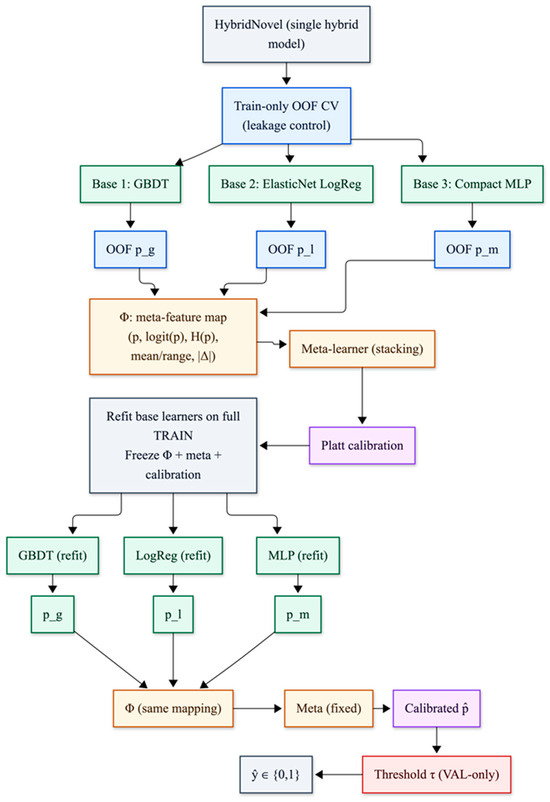
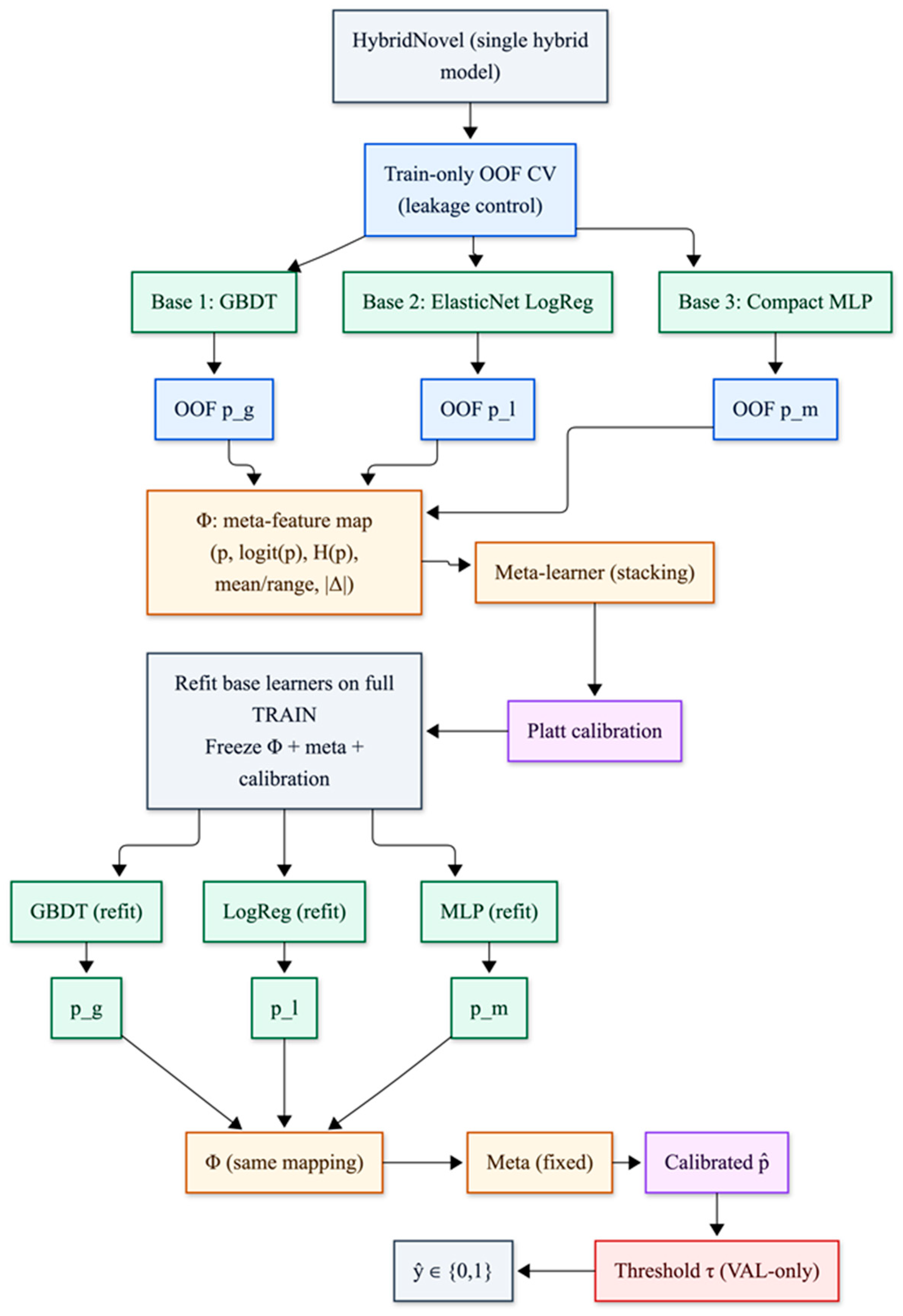
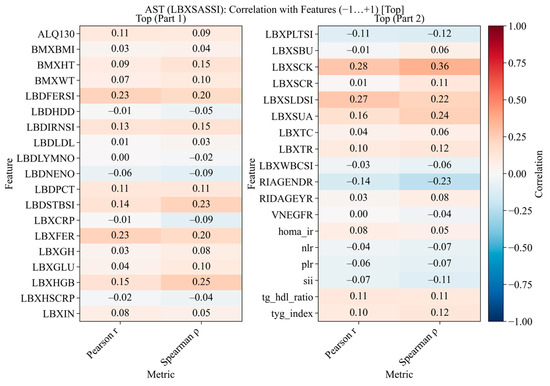
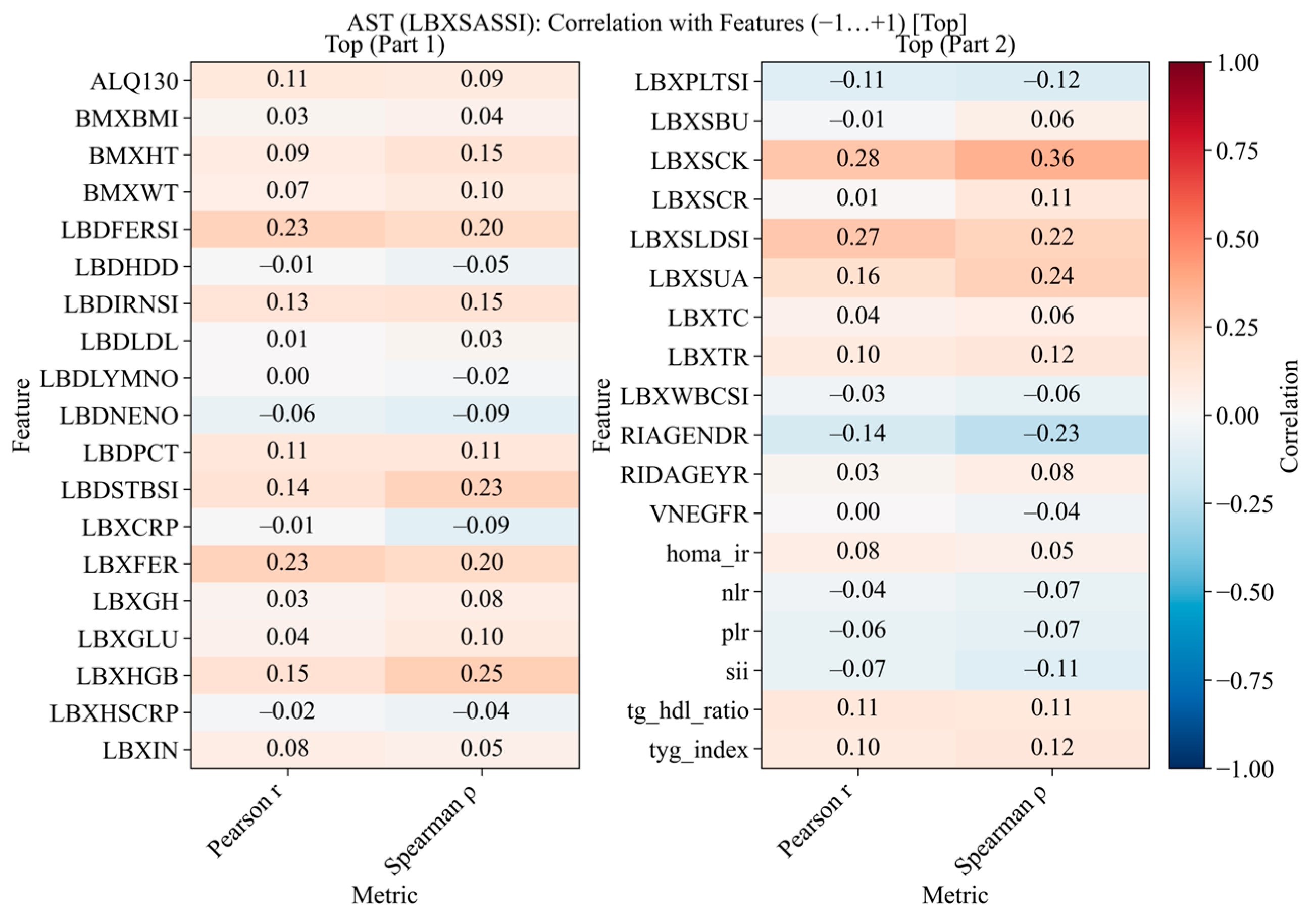
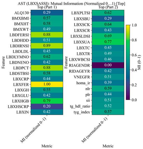
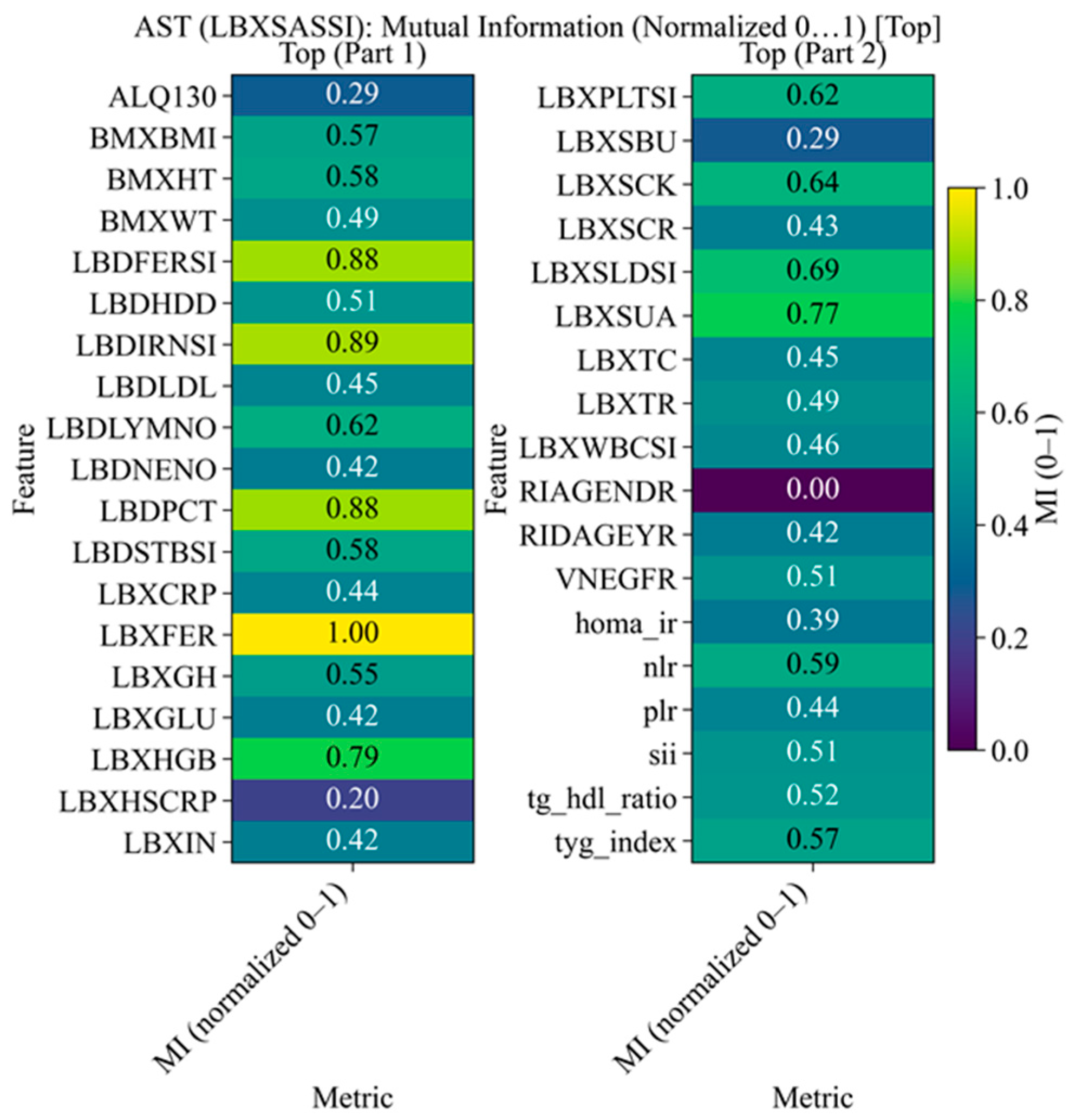
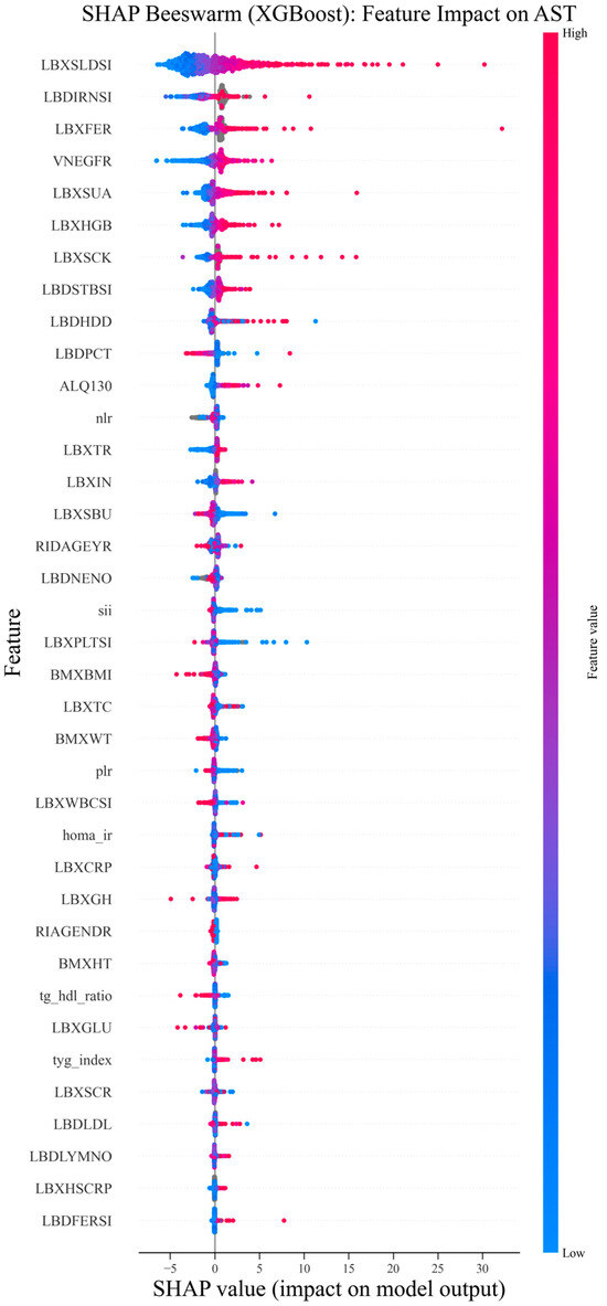
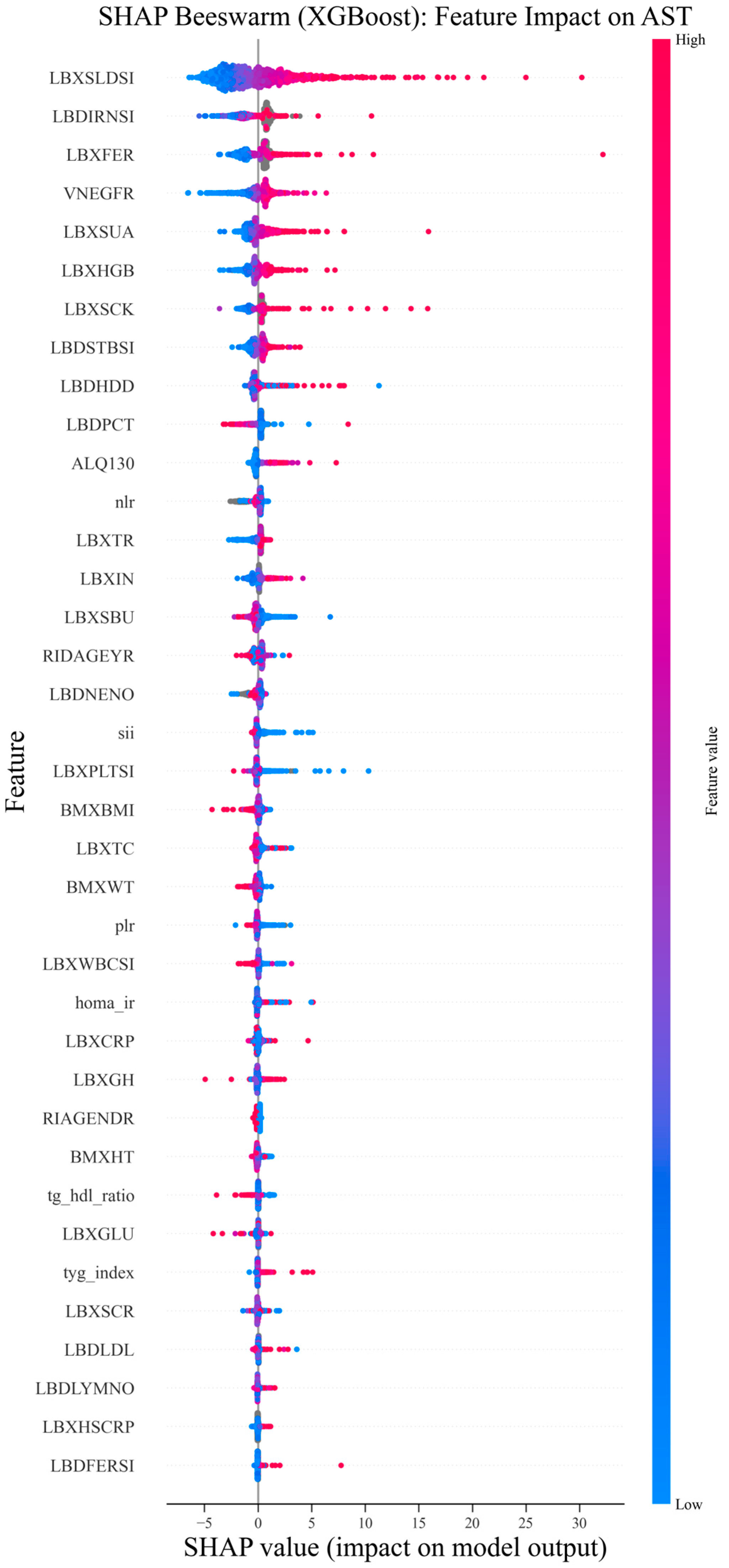
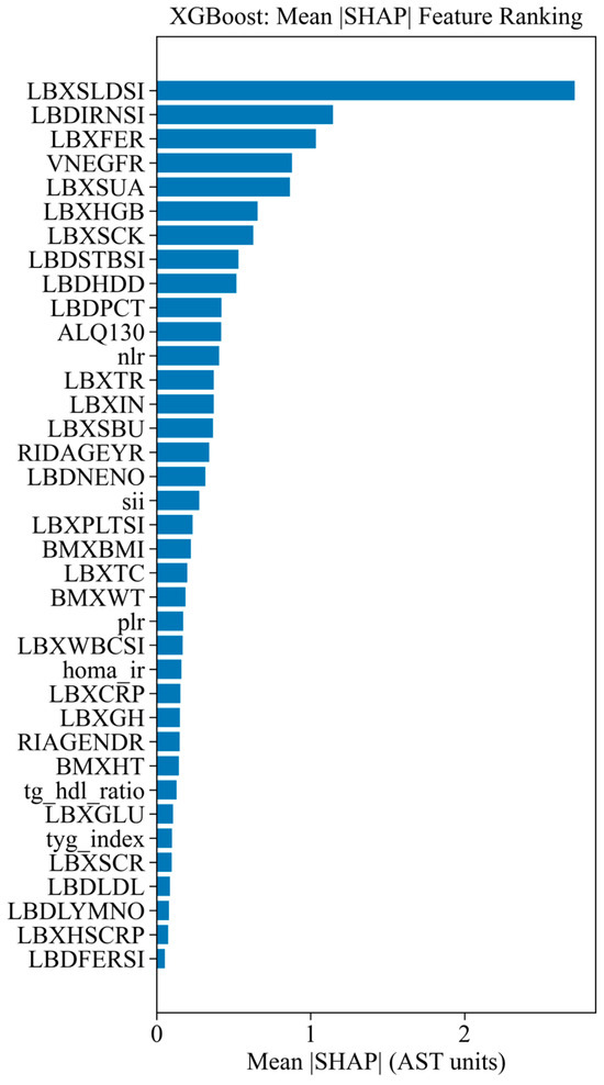
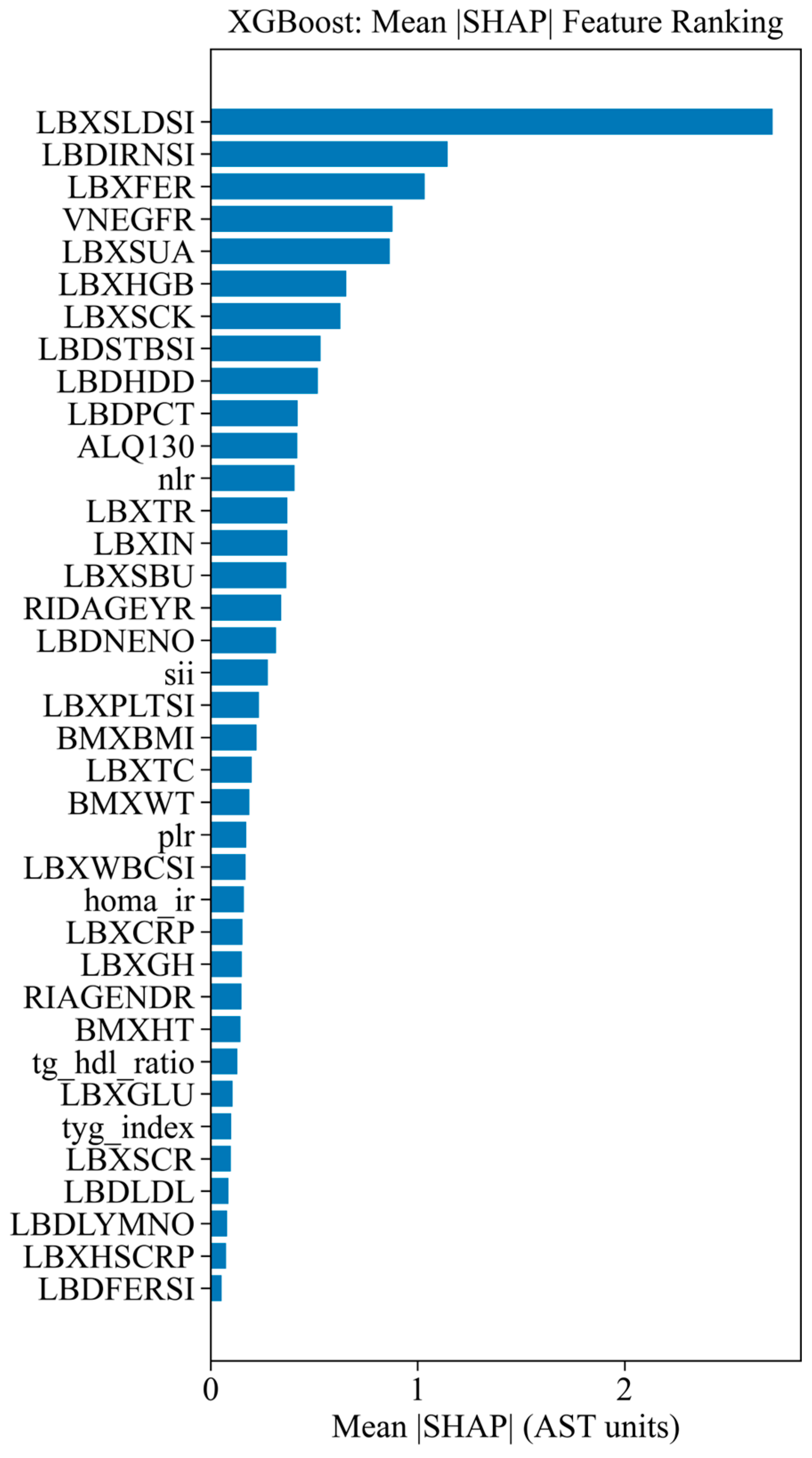
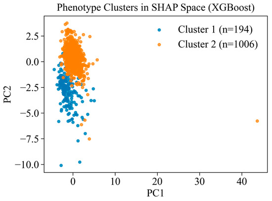
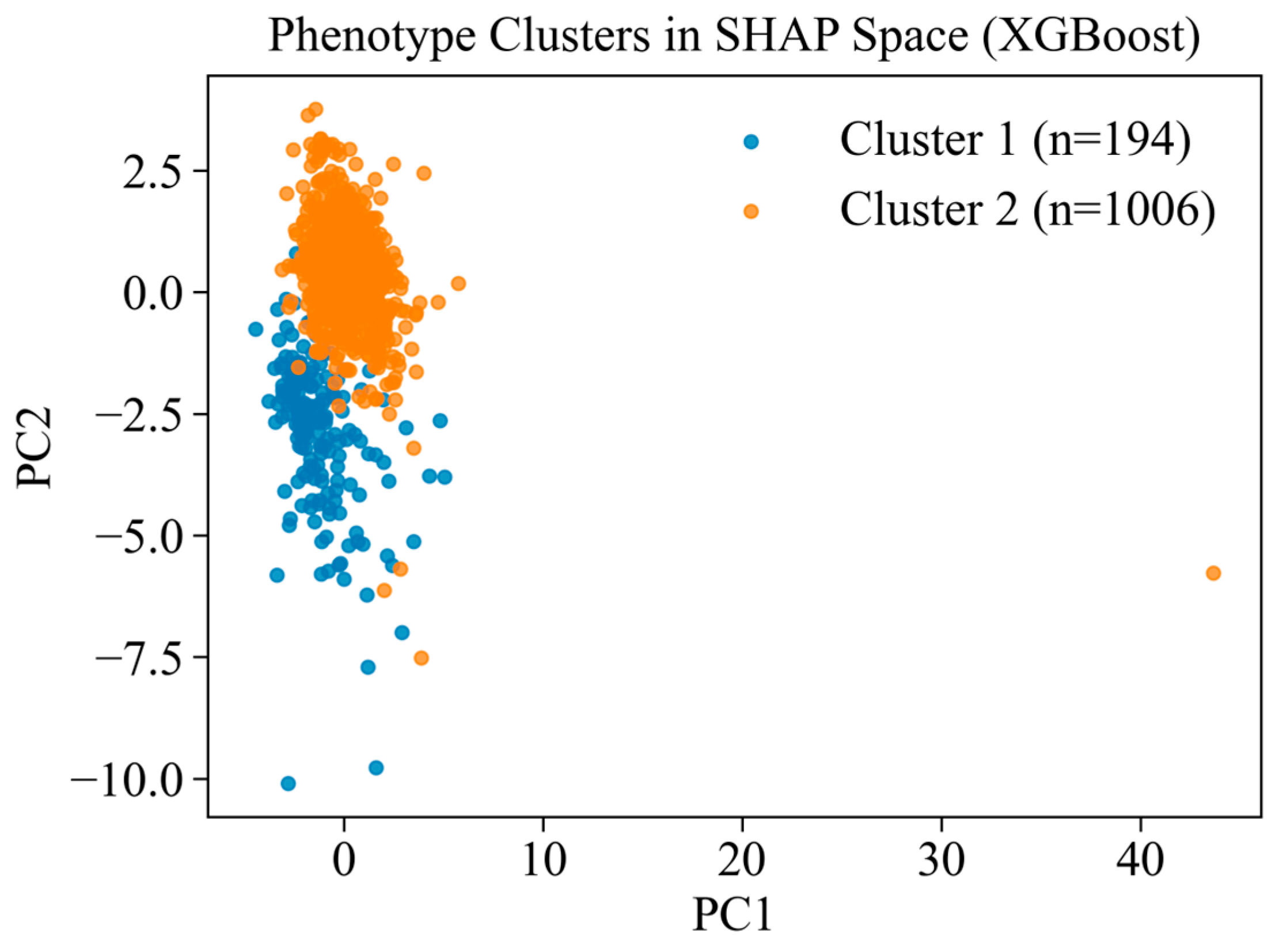
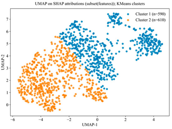
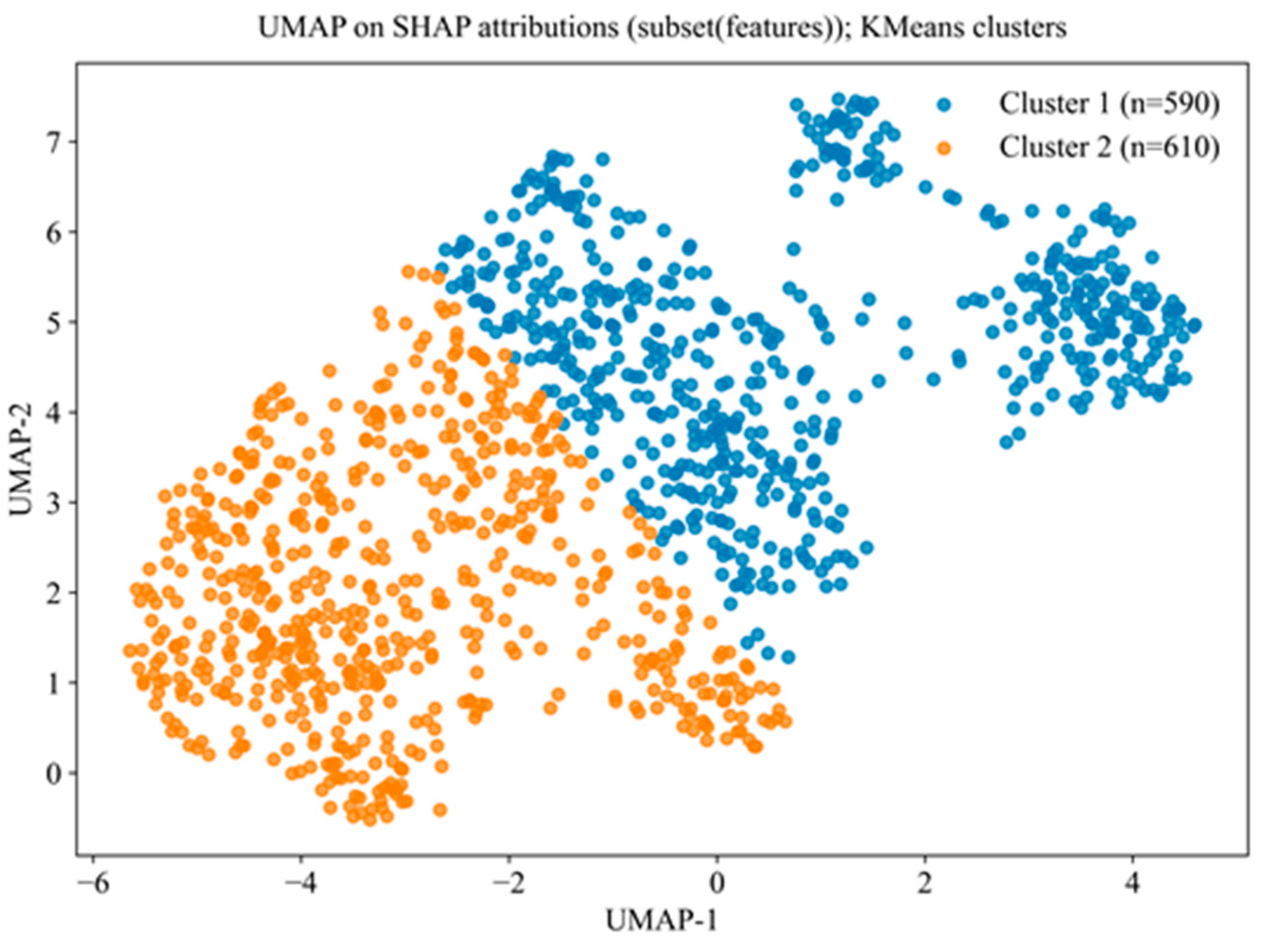
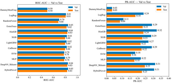
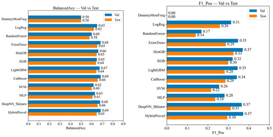
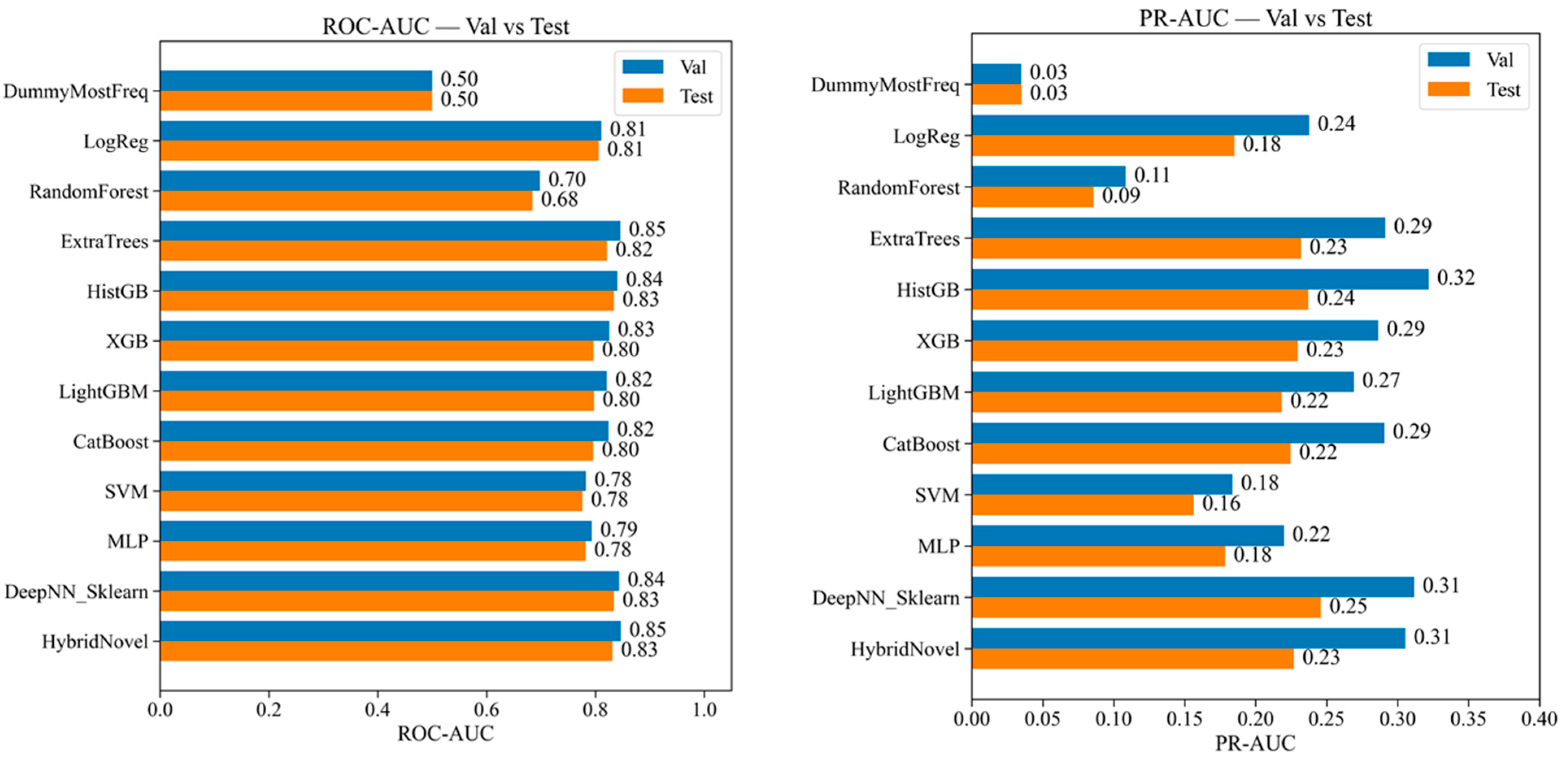
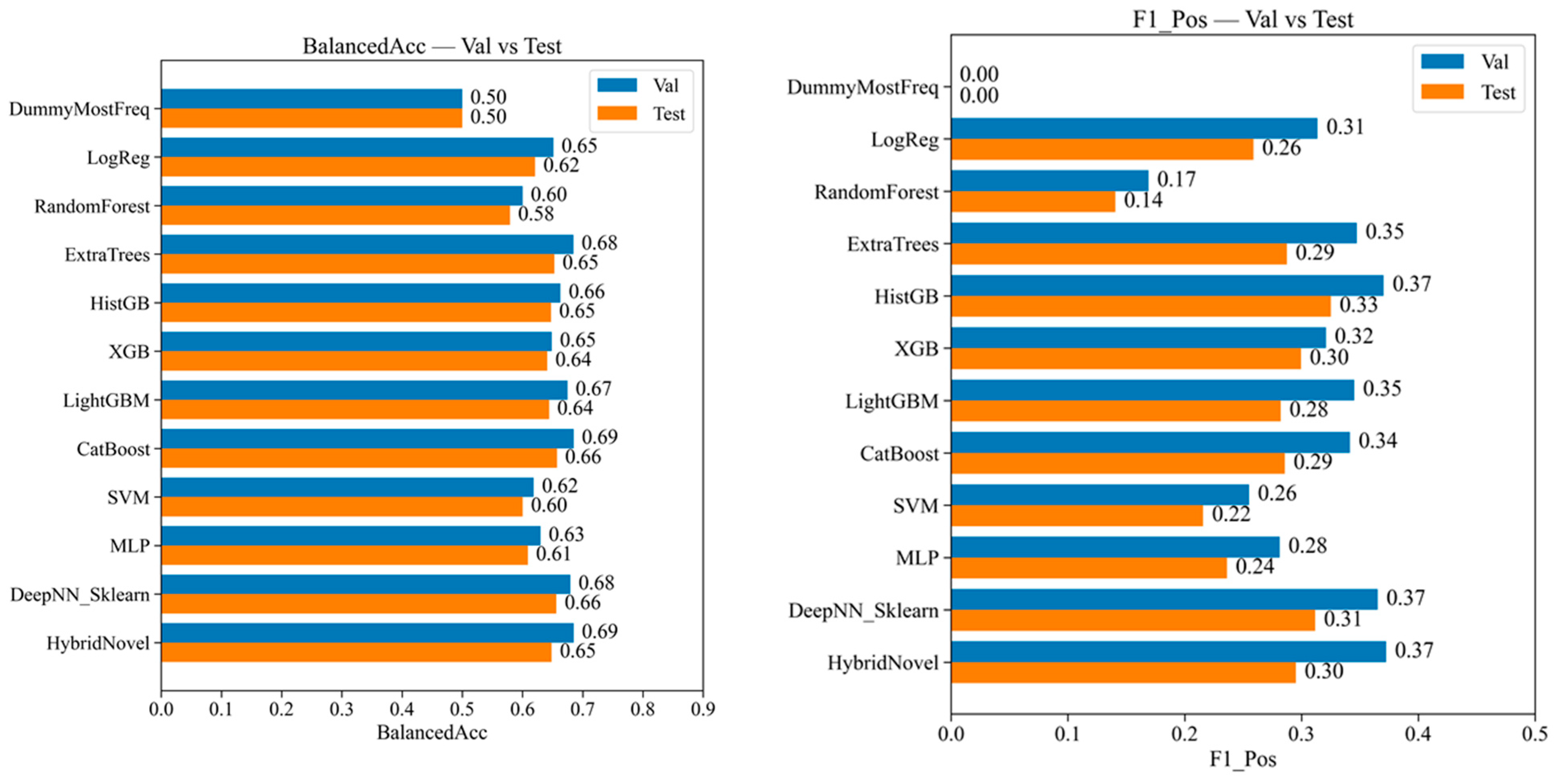
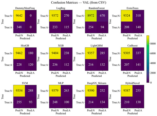
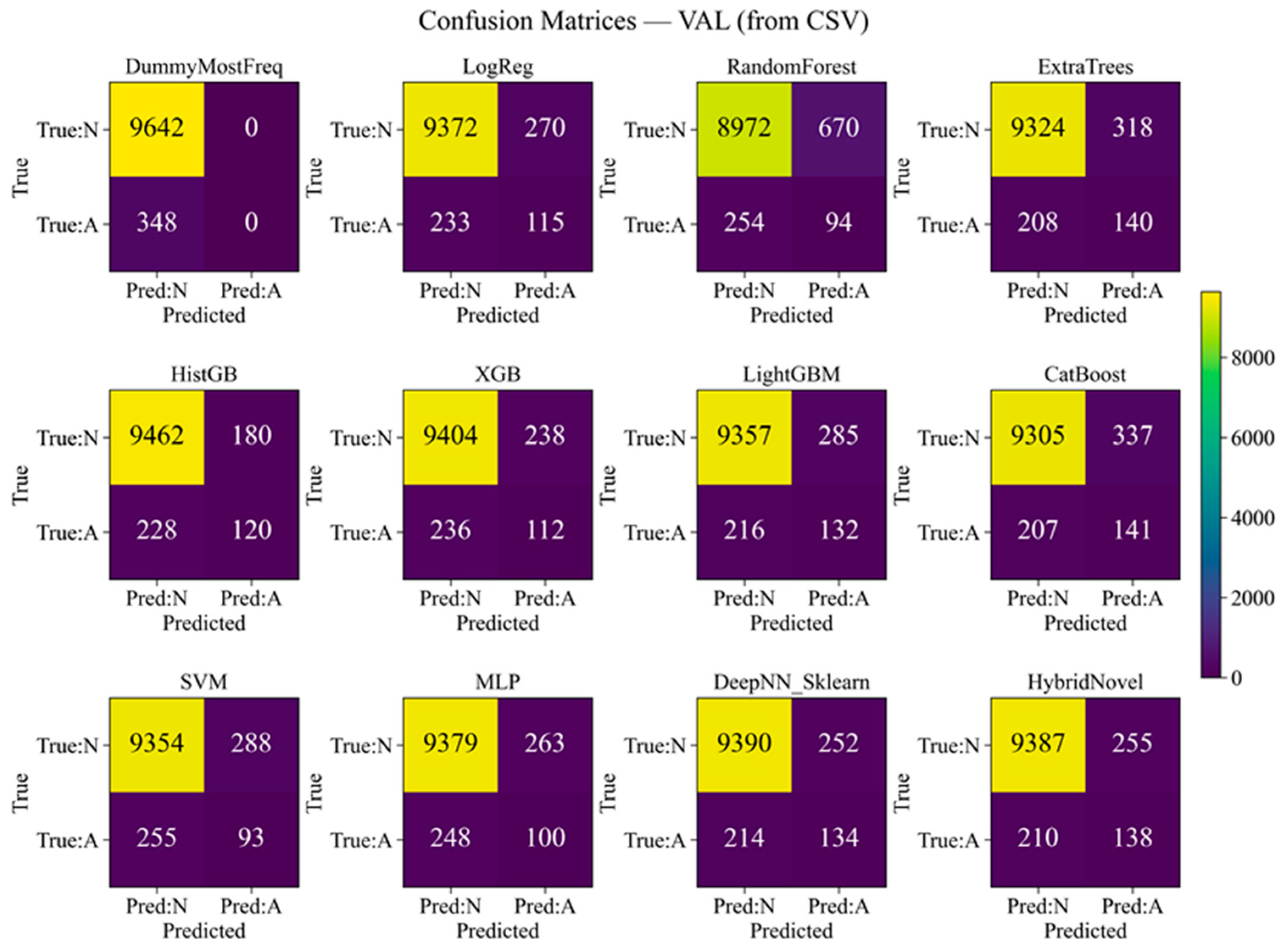
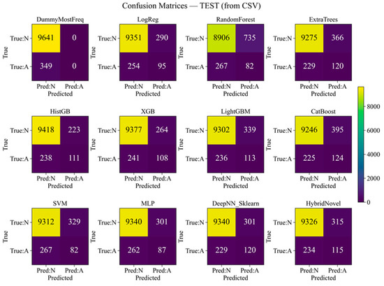
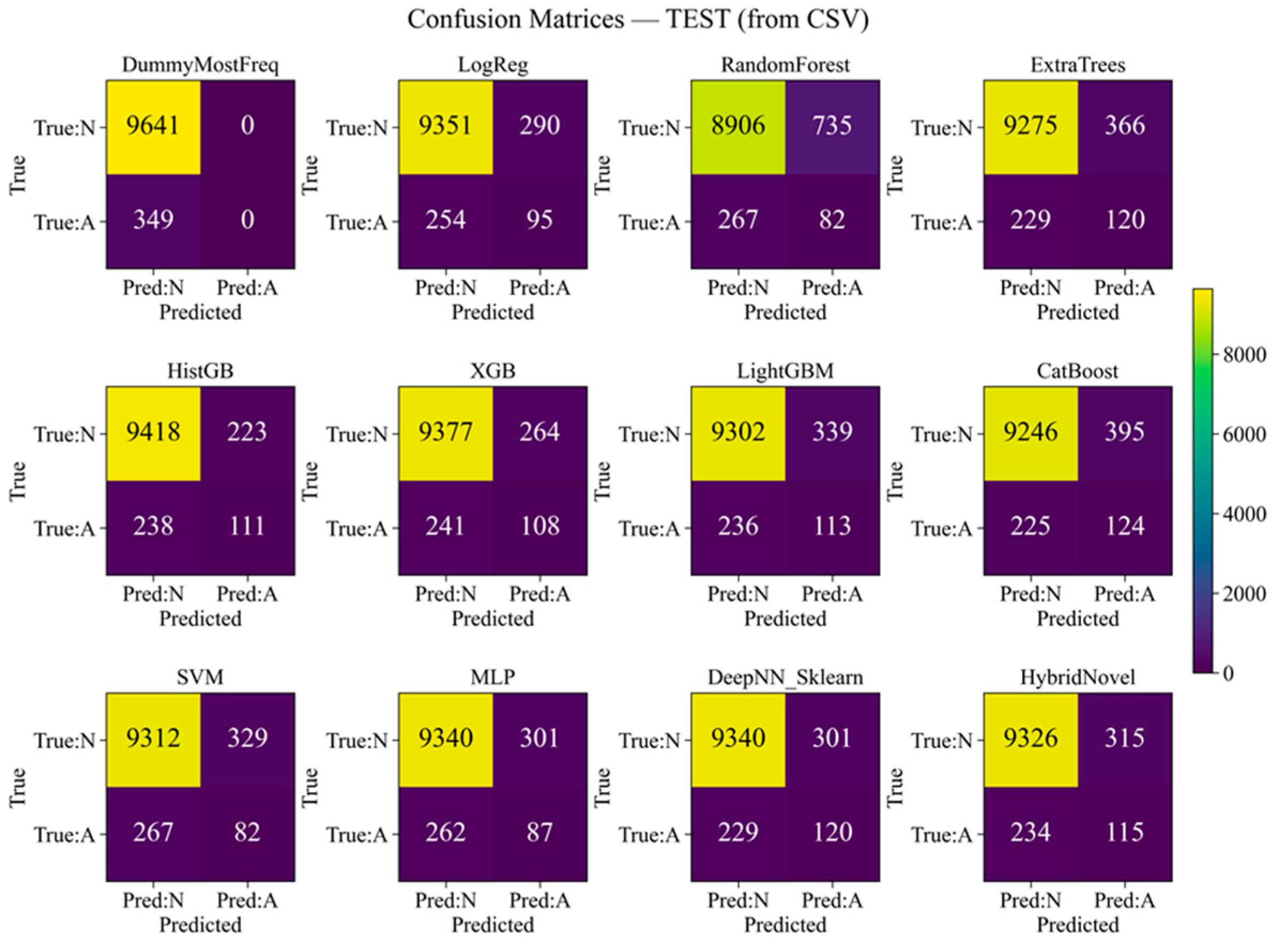

Disclaimer/Publisher’s Note: The statements, opinions and data contained in all publications are solely those of the individual author(s) and contributor(s) and not of MDPI and/or the editor(s). MDPI and/or the editor(s) disclaim responsibility for any injury to people or property resulting from any ideas, methods, instructions or products referred to in the content. |
© 2026 by the authors. Licensee MDPI, Basel, Switzerland. This article is an open access article distributed under the terms and conditions of the Creative Commons Attribution (CC BY) license.