


Abstract
The network fabric of geographically distributed high-throughput computing (HTC) clusters has become a critical factor in supporting large-scale scientific workflows, yet job-level data transfer behavior in production batch systems remains insufficiently understood. In this paper, we present a measurement and predictability study of HTCondor-recorded job-level transfer behavior using a 14-month production dataset comprising 757,868 real jobs from the geographically distributed HTCondor cluster at the Institute of High Energy Physics (IHEP). Our analysis reveals a pronounced directional asymmetry in recorded job-level transfer behavior when measured by job count: 88.4% of jobs exhibit only input-side transfer, while 92.9% generate zero output-side transfer. By applying unsupervised clustering as an exploratory labeling tool, we derive empirical labels for seven input-side transfer patterns and three output-side transfer patterns, revealing both dominant low-transfer populations and rare high-transfer groups. We further use lightweight job information available at submission time to examine whether these discovered transfer patterns can be predicted before execution. The results show that input-side transfer patterns are partially predictable from job semantics such as job type, accounting group, and command-line arguments, while output-side prediction is largely constrained by severe class imbalance and dominant job-type regularities. Overall, the results provide empirical evidence that job-level transfer behavior in a real geographically distributed HTC environment is structured, directionally asymmetric, and partially predictable before execution. These findings offer lightweight transfer-awareness signals for future studies of data-locality-aware site ranking, cache preparation, storage layout planning, and transfer-aware resource management in large-scale HTC systems.
1. Introduction
High-throughput computing (HTC) has become the de facto standard paradigm in data-intensive scientific domains such as high-energy physics [1]. Workloads in such scenarios typically consist of massive numbers of mutually independent file-level tasks, exhibiting a highly parallelizable nature. Unlike high-performance computing (HPC), which pursues the shortest completion time for a single job, HTC focuses on completing as many jobs as possible within a given time window, so as to maximize overall throughput [2,3].
The Institute of High Energy Physics, Chinese Academy of Sciences (IHEP) operates and maintains a geographically distributed HTC cluster, which serves as the core computing node of the National High Energy Physics Science Data Center [4]. The cluster comprises approximately 80,000 x86 CPU cores, nearly 10,000 ARM CPU cores, about 200 GPU cards, and more than 119 PB of storage resources, distributed across Beijing, Dongguan, several experimental facility sites, and university edge stations. Taking large-scale experiments such as LHAASO and BESIII as examples, scientific computing must be carried out collaboratively across the northern and southern centers, while data placement, remote access, and job execution may span different geographic locations. In such a production environment, data movement becomes an important factor in workload management, resource coordination, and network-aware scheduling.
This setting motivates a basic empirical question: whether job-level transfer behavior in geographically distributed HTC environments is directionally symmetric, or whether input-side and output-side transfers exhibit different distributions. This question is relevant to network-aware scheduling and resource planning, because directionally asymmetric transfer behavior may require different treatment from a single aggregate I/O metric. Therefore, this paper focuses on characterizing the directional structure, empirical modes, and submission-time predictability of job-level transfer behavior recorded in the IHEP production HTCondor environment.
Regarding job behavior characterization, existing work predominantly focuses on computational resource dimensions such as CPU, memory, disk, and execution time [5,6], paying comparatively limited attention to network behavior. For instance, Banjongkan et al. [7] demonstrates the viability of submission-time prediction by utilizing three user-specified attributes—user ID, requested CPU cores, and queue type—to forecast final job status (finished vs. failed). Furthermore, existing studies typically treat job data transfers monolithically as aggregate I/O behavior [8,9], largely overlooking the fundamental differences between input traffic (e.g., fetching raw data) and output traffic (e.g., writing back computational results) in terms of distributional characteristics and predictability. Meanwhile, established network traffic forecasting methods [10,11,12], though widely applied to link- and aggregate-level prediction, rely heavily on historical time-series data or runtime telemetry; consequently, they cannot facilitate proactive planning prior to scheduling decisions.
To address the above problems, this paper conducts a systematic measurement and predictability study of job-level transfer behavior based on 14 months of production operation data from the IHEP geographically distributed HTC cluster. Unless otherwise specified, job-level traffic in this paper refers to HTCondor-reported transfer bytes recorded by BytesRecvd and BytesSent, rather than complete end-to-end network traffic. The main contributions of this paper are as follows:
- Production-scale measurement of directional asymmetry in HTC job transfer behavior. Based on a dataset containing 757,868 real job records, we find that input-side and output-side transfers exhibit discrete, multimodal distribution patterns. At the level of job-count proportions, 88.4% of jobs are input-only, and 92.9% of jobs generate zero output-side transfer. This finding shows that recorded job-level transfer behavior is strongly asymmetric in terms of transfer occurrence and direction patterns, providing a basis for analyzing input-side and output-side transfers as separate dimensions.
- Characterization of empirical input-side and output-side transfer patterns. Using unsupervised density-based clustering as an exploratory labeling tool, we identify seven non-noise input-side transfer patterns and three non-noise output-side transfer patterns under the selected HDBSCAN settings. The output direction is much more concentrated, with the largest output-side pattern accounting for 99.2% of jobs. These results indicate that input-side and output-side transfer behavior exhibit different empirical distributional structures and should be analyzed as two related but distinct dimensions of job behavior.
- Evidence that empirical transfer patterns are associated with job semantics. Feature importance and ablation analyses show that command-line arguments, accounting groups, and job types provide the dominant predictive signals. This suggests that the derived empirical transfer-pattern labels reflect recurring job templates, experiment groups, and workflow semantics in addition to byte-count differences.
- A priori predictability analysis and its boundary. We evaluate whether post-execution transfer patterns can be inferred from lightweight submission-time attributes under a shared prediction protocol. The results show that input-side transfer patterns are strongly predictable, whereas output-side transfer-pattern prediction is more sensitive to severe class imbalance and requires per-class recall and confusion-matrix analysis in addition to aggregate accuracy. Robustness tests and job-template holdout evaluation further characterize the boundary of submission-time predictability.
- Implications for lightweight transfer-aware scheduling. Rather than relying on heavyweight runtime telemetry alone, the observed semantic regularities suggest that lightweight scheduler-side rules or compact submission-time predictors may help provide early transfer-awareness signals for data placement, cache preparation, and candidate-site ranking. At the same time, rare high-transfer patterns should be handled conservatively because their operational impact depends not only on transferred bytes, but also on transfer duration, concurrency, and site-level data-access paths.
Overall, these findings provide empirical evidence for understanding and exploiting the regularity of HTC job transfer behavior. The measured asymmetry suggests that input and output transfer demands should not be treated as identical dimensions in capacity planning. The semantic predictability of transfer patterns further suggests that lightweight scheduler-side rules or compact predictors may help inform data placement, cache preparation, and candidate-site ranking. At the same time, the output direction reveals a clear risk-sensitive boundary: rare high-output transfer patterns require recall-oriented or conservative handling rather than evaluation based only on aggregate accuracy.
The remainder of this paper is organized as follows: Section 2 reviews related research on HTC workload modeling, network awareness, and network traffic prediction; Section 3 introduces the dataset construction, transfer-direction pattern definition, unsupervised transfer-pattern discovery, and supervised prediction methods; Section 4 presents the results of the statistical analysis, pattern discovery, and prediction experiments; and Section 5 concludes the paper and discusses future work.
2. Related Work
2.1. HTC/HPC Job Characterization and Prediction
The characterization and modeling of high-throughput computing (HTC) jobs has long been a research focus in the field of system optimization. Early studies mainly concentrated on the resource demand characteristics of jobs, such as CPU, memory, and disk usage as well as runtime. Silva et al. [13] conducted a characterization analysis of the HTC workload of the CMS experiment at the Large Hadron Collider (LHC), applying statistical recursive partitioning and conditional inference trees to identify patterns in job runtime, disk usage, and memory usage, and proposed resource demand estimation methods based on regression trees and probability distributions, achieving an average accuracy of 75% for runtime prediction. Xu et al. [14] combined classification with instance-based learning, predicting job execution time by matching historically similar jobs and using a genetic algorithm to optimize parameters. However, these studies are largely confined to the computing resource dimension, and their characterization of job network behavior is clearly insufficient.
With respect to job behavior clustering, Halawa et al. [15] proposed an unsupervised job clustering method based on key performance indicators (KPIs), using a real HPC dataset from the CESGA supercomputing center to perform clustering analysis over multiple categories of monitoring metrics, including CPU, memory, and network interface traffic. Notably, their experimental results show that network-interface-traffic-related KPIs can provide better intra-cluster cohesion and inter-cluster separation than CPU or memory metrics, indicating that network behavior is of significant value for distinguishing types of computing jobs. That work, however, targets runtime monitoring data from an HPC data center and relies on real-time KPI time series collected during job execution.
2.2. Network Awareness in Distributed Systems
In distributed computing infrastructures, awareness of network resource status plays a critical role in system performance optimization. Existing research has explored the influence of network factors on job execution efficiency from various perspectives. Javadi and Matawie [16] performed statistical modeling of resource availability in volunteer computing systems, using models such as MAP, MMPP, and MWM to fit the long-range dependence characteristics of system-level resources, revealing that the temporal correlation of network resource availability offers valuable reference for system capacity planning. Moon et al. [17] pointed out, in a P2P distributed computing setting, that processing capability and network transmission capability jointly determine the end-to-end completion time of a job, and that network capacity should therefore be regarded as a class of infrastructure resource equally important as computing capability; their method, however, relies on dynamically probing node processing capability and network bandwidth at runtime. Zhang et al. [18] integrated Linux containers and virtual Ethernet devices into the HTCondor system, achieving job-level network isolation and bandwidth management, thereby verifying from an engineering standpoint the feasibility of fine-grained network resource control in HTC clusters; that solution, however, allocates a fixed amount of bandwidth to each job, cannot adapt to the dynamic changes in bandwidth demand that occur during the actual execution of high-energy physics jobs, and lacks any mechanism for estimating bandwidth demand before a job runs. Timilsina and Shannigrahi [19] proposed a network-aware framework based on real-time telemetry data that predicts job completion time on candidate nodes using runtime monitoring data, improving the accuracy of optimal node selection by 34–54% compared with the default Kubernetes scheduler, thus demonstrating in practice the significant value of network status information for job placement decisions.
Taken together, the works above show that awareness of network resource status is a key component of performance optimization in distributed systems. However, such information is usually obtained either through dynamic runtime acquisition, such as telemetry and real-time probing, or through fixed a priori configuration, such as pre-allocated bandwidth. In the production HTCondor setting considered in this paper, an important remaining question is whether job-level transfer behavior recorded by the scheduler can be characterized in terms of input-side and output-side directions, and whether the resulting directional transfer patterns can be inferred before execution from lightweight submission-time information. This motivates our study of submission-time predictability for HTCondor-recorded job-level transfer patterns, with a particular focus on the directional behavior represented by BytesRecvd and BytesSent.
2.3. Network Traffic Prediction Methods
Network traffic prediction has been widely applied to resource allocation, congestion control, and capacity planning. Early approaches mostly adopted statistical time-series methods such as ARIMA, exponential smoothing, and regression models, but such methods rely on stationarity assumptions and struggle to capture the nonlinearity, burstiness, and long-range dependence present in network traffic. In recent years, deep learning methods have gradually become mainstream: Trinh et al. [20] used LSTM to predict LTE base station traffic; Lazaris and Prasanna [21] proposed an LSTM prediction framework based on real ISP network traces; and Azari et al. [22] compared LSTM with ARIMA for cellular traffic prediction, with results showing that deep learning models generally possess stronger temporal modeling capability. Ferreira et al. [23] further provided a systematic survey of network traffic prediction methods, noting that deep learning models have advantages in modeling complex traffic patterns, but that their performance often depends on large volumes of historical traffic data and careful model tuning.
Although the above methods have achieved good results in link-level, base-station-level, or aggregate-level time-series prediction, they have two limitations in the context of HTC job management. First, these methods rely on historical traffic observations or runtime network telemetry data, and thus cannot make predictions at job submission time, when no runtime transfer information has yet been generated. Second, most existing studies model job-level data movement as a single aggregate quantity and seldom distinguish the differences between input-side and output-side transfers in terms of operating mechanism, distributional characteristics, and predictability.
3. Methodology
3.1. Dataset Construction
The data used in this paper were collected from the geographically distributed HTC cluster of the Institute of High Energy Physics, Chinese Academy of Sciences, which spans multiple data centers, with the raw records originating from HTCondor job logs. The dataset covers operational records from November 2024 to December 2025. Since the raw logs use the subtask as their smallest unit, whereas both actual scheduling and performance analysis are conducted at the job level, we aggregated subtasks into job-level samples according to cluster_id, obtaining a total of 757,868 valid jobs. During preprocessing, anomalous samples with missing key fields were removed. The input and output transfer bytes used in this study are derived from the HTCondor BytesRecvd and BytesSent counters, respectively. These counters record bytes transferred through the HTCondor shadow-starter communication channel. Therefore, the measured fields represent HTCondor-recorded job transfer volume rather than complete packet-level or end-to-end job network traffic.
It should be noted that this dataset represents a production HTCondor workload from a single institution, IHEP, and is mainly associated with high-energy physics applications. Therefore, the empirical observations derived from this dataset characterize the studied IHEP distributed HTC environment rather than all HTC systems. The measurement and prediction workflow used in this paper is intended to be applicable to other HTC environments, but the specific transfer distributions and mode proportions may vary with scientific domain, data-management policy, and scheduler configuration.
Table 1 lists the name and meaning of each category of fields, together with their uses in this paper. The aggregated dataset contains 17 fields, which are divided into three categories according to the analysis stage in which they are used:
Table 1.
Dataset feature categories and examples.
- Identifier feature: cluster_id, used to uniquely identify each job-level sample.
- Prediction features: prefixed with pred_, these are static pieces of information that can be obtained directly from the user’s submission description file before a job is submitted, including the task scale of the job, the resource requests of its subtasks, the job type, and the accounting group. They are used to build the prediction model.
- Post-execution measured transfer features: prefixed with valid_, these are the measured results obtained after job completion, covering job-level input/output transfer bytes as well as the statistical distribution of subtask-level input/output transfer bytes.
It should be noted that the valid_ fields are used only to characterize post-execution HTCondor-recorded transfer behavior, and serve for transfer-direction definition, clustering-based transfer-pattern discovery, and supervised learning label construction. In the submission-time transfer-pattern prediction stage, the model input contains only the pred_ fields, so as to avoid data leakage caused by the use of post-execution information.
Dividing the fields into prediction features and post-execution measurement features makes it possible to distinguish the information available before job submission from the measured transfer information used after execution. This supports subsequent analysis of recorded transfer-pattern structure and submission-time predictability. In addition, to capture internal variation among subtasks, we extracted the minimum, median, 95th percentile, and maximum values of the task-level input-side and output-side transfer bytes. These statistics characterize both cross-subtask variation and high-percentile transfer behavior, thereby providing a finer-grained feature foundation for subsequent transfer-pattern discovery and prediction modeling.
3.2. Job-Level Transfer-Direction Pattern Definition
This section defines a directional classification method for job-level transfer behavior. Specifically, we first extract input-side and output-side transfer byte counts from the HTCondor log-derived fields, and then classify jobs into several well-defined transfer-direction patterns based on their zero-value status and input-to-output ratio.
- 1.
- Definition of Job-level Transfer Metrics
We first extract the following job-level transfer fields from the HTCondor logs:
- valid_cluster_network_in_bytes: input-side transfer bytes derived from the HTCondor BytesRecvd attribute;
- valid_cluster_network_out_bytes: output-side transfer bytes derived from the HTCondor BytesSent attribute.
Based on these two fields, the input–output transfer ratio is further calculated: , where represents input-side transfer bytes and represents output-side transfer bytes. When , the ratio is not calculated, and the job is directly assigned to zero-output related categories.
- 2.
- Transfer Directionality Classification
To characterize the directionality of job-level transfer behavior, we define six rule-based transfer-direction patterns according to the presence or absence of input/output transfer bytes and their ratio, as shown in Table 2. Let and denote the input-side and output-side transfer bytes of a job, respectively. If both are zero, the job is labeled as having no recorded transfer. If only input-side transfer or only output-side transfer is present, the job is labeled as input-only or output-only, respectively. For jobs with both input-side and output-side transfers, we calculate . When , the job is considered balanced type; when , it is considered input-dominant type; when , it is considered output-dominant type.
Table 2.
Rule-based definitions of job-level transfer-direction patterns.
In the subdivision of bidirectional transfers, we use the input–output byte ratio R as the classification indicator, defining as balanced type, meaning that input-side and output-side transfer volumes are of the same order of magnitude. When , the job is classified as input-dominant; when , it is classified as output-dominant. This threshold helps distinguish jobs with clearly asymmetric transfer directions while avoiding the misclassification of jobs with only negligible reverse-side transfer as balanced.
It should be noted that the rule-based transfer-direction patterns described above and the clustering findings presented later in Section 3.3 answer questions at different levels. The direction patterns describe the presence or absence of input/output transfer and their relative proportion, whereas the clustering findings describe the magnitude tiers of transfer volume within each direction. Together, the two provide a structured characterization of job-level transfer behavior.
In this paper, clustering is performed independently on input-side and output-side transfers for two reasons. First, the distributional shapes of input-side and output-side transfer volumes differ significantly, and joint clustering would obscure their respective structures. Second, input-side and output-side transfers may reflect different operational processes in HTCondor-managed jobs, and should therefore be analyzed as separate dimensions.
3.3. Unsupervised Transfer-Mode Discovery
Different from the rule-based transfer-direction patterns defined in Section 3.2, this section discovers data-driven transfer patterns from post-execution transfer statistics using unsupervised clustering. The rule-based direction patterns describe whether a job has input-side transfer, output-side transfer, or both, whereas the clustering-based transfer patterns further characterize the scale and distributional structure within each transfer direction.
For each job, we construct direction-specific transfer feature vectors for input-side and output-side transfers, respectively, using the post-execution measurement features listed in Table 1. Each direction-specific feature vector includes the job-level total transfer volume and four subtask-level statistical features, namely the minimum, median, 95th percentile, and maximum transfer volume across subtasks. The job-level total transfer volume captures the overall data-movement scale, whereas the subtask-level statistics characterize dispersion and long-tail behavior across subtasks. This feature design avoids relying on the mean alone, which may obscure extreme subtask-level discrepancies in highly skewed HTC transfer distributions.
Before clustering, numerical missing values are imputed using the median. The nonlinear transformation rule is evaluated independently for each of the five selected transfer-volume features in each direction. Specifically, we apply a Yeo–Johnson power transformation only to transfer features that are strictly positive in the analyzed data and have an absolute skewness greater than 1. Features that do not satisfy these positivity and skewness conditions are kept unchanged before standardization. All selected transfer features are then standardized using z-score normalization. Consistent with the rationale discussed above, input-side and output-side feature matrices are clustered independently.
In terms of clustering workflow, HDBSCAN is applied to the standardized transfer feature matrices using the Euclidean distance metric. The purpose of using HDBSCAN is to derive data-driven empirical transfer-pattern labels while allowing samples that cannot be robustly assigned to any sufficiently dense region to be labeled as noise. In the HDBSCAN results, samples labeled as are treated as noise samples and are not interpreted as regular transfer patterns. Therefore, the reported number of transfer patterns refers only to non-noise HDBSCAN clusters.
To determine the HDBSCAN parameters, we conducted a grid-based diagnostic screening over three key parameters: min_cluster_size, min_samples, and cluster_selection_epsilon. The candidate values were
For each candidate setting, we recorded the number of non-noise clusters, the noise proportion, and conventional internal validation metrics, including the Silhouette coefficient, Calinski–Harabasz index, and Davies–Bouldin index. These conventional metrics were used as auxiliary indicators of compactness and separation, but were not interpreted alone because the transfer feature space contains highly repeated values and highly skewed distributions. The final direction-specific setting was selected through a multi-diagnostic assessment of the initial screening results, considering the number of non-noise patterns, noise behavior, conventional internal metrics, and the interpretability of the resulting transfer tiers, rather than relying solely on conventional internal metrics. The selected settings are summarized in Table 3.
Table 3.
Final direction-specific HDBSCAN settings used for transfer-pattern discovery.
After the final HDBSCAN labels were obtained, we computed the density-based clustering validation index (DBCV) using a stratified sample constructed from the final label distribution. The DBCV calculation used at most 30,000 samples, with a minimum target of 1000 records per label when available, and random seed 42. We also evaluated final-label reproducibility through repeated stratified subsampling. In each repeat, HDBSCAN was refitted on a stratified subsample using the selected parameter setting, and the resulting labels were compared with the corresponding labels from the full-data clustering using Adjusted Rand Index (ARI) and Normalized Mutual Information (NMI). For both input-side and output-side transfers, we used three repetitions with random seeds 42, 43, and 44. Each repetition sampled at most 100,000 records, corresponding to an 80% stratified subsample subject to this cap, with a minimum target of 1000 records per label when available. These metrics assess whether the derived labels are reproducible under sampling perturbations for the selected parameter setting. This analysis is distinct from sensitivity to alternative HDBSCAN parameter choices, which is addressed through the initial parameter screening procedure.
Finally, to examine how the HDBSCAN-derived labels differ from a simple rule-based scale partition, we compare them with a granularity-matched log-scale binning baseline constructed from the corresponding job-level transfer volume. The agreement between HDBSCAN-derived labels and the log-scale binning baseline is evaluated using both ARI and NMI, so that chance-adjusted label agreement and information-theoretic consistency are considered together. This comparison is used to characterize differences between the two partitioning strategies rather than as a performance ranking of the labeling methods.
The complete unsupervised transfer-mode discovery procedure is summarized in Algorithm 1.
| Algorithm 1 Unsupervised Transfer-Mode Discovery Using HDBSCAN |
|
3.4. Supervised Transfer-Pattern Prediction
Due to the pronounced long-tail distribution and multimodal characteristics of job-level transfer bytes, directly predicting continuous transfer volume is sensitive to extreme samples and may provide limited interpretability for resource management decisions. We therefore formulate the problem as transfer-pattern prediction: the post-execution transfer patterns discovered in Section 3.3 are used as supervised learning targets, and the corresponding pattern label is predicted from information available at job submission time.
This formulation assumes that submission-time parameters, such as command-line arguments, job types, and resource requests, may contain useful signals about subsequent input-side and output-side transfer patterns. The input features include six static fields: requested number of processes, requested number of CPUs, requested memory, job type, accounting group, and command-line arguments.
The transfer-pattern labels are generated in the preceding offline transfer-pattern discovery stage using post-execution transfer records.
The supervised prediction pipeline is designed as a shared protocol for assessing a priori predictability rather than as a direction-specific model optimization framework. The same submission-time feature set, feature engineering strategy, data-splitting scheme, and modeling procedure are applied to both input-side and output-side transfer patterns. This design allows the predictability of the two transfer directions to be compared under a consistent experimental protocol.
For the supervised prediction stage, raw submission-time records are divided into training and test partitions before any data-dependent preprocessing is fitted. All preprocessing components, including imputation statistics, categorical encoders, rare-category rules, target-encoding statistics, and the TF–IDF vectorizer for command-line arguments, are estimated from the training partition only and then applied unchanged to the test partition. Numerical features are standardized, categorical features are encoded using frequency encoding, rare-category merging, hierarchical feature extraction, categorical mappings, and target encoding, while command-line arguments are converted into sparse TF–IDF features. Considering the significant class imbalance in transfer-mode distribution, accuracy, Weighted F1, Macro F1, per-class precision, per-class recall, per-class F1, and confusion matrices are used for performance evaluation. Among these metrics, Macro F1 and per-class recall are used to assess recognition capability for minority transfer patterns, whereas per-class precision and F1 are used to identify whether improved minority recall is accompanied by increased false assignments to minority classes.
The supervised prediction stage is evaluated under three train–test partitioning protocols. The primary protocol is an 80:20 stratified random split, which estimates in-distribution predictive performance while preserving the label distribution. The second protocol is an order-based holdout split: jobs are sorted by the available monotonic job identifier, with the earlier 80% used for training and the later 20% used for testing. Because reliable timestamp fields are not available in the prediction table, this protocol is treated as an order-based temporal proxy. The third protocol is a job-template group-holdout split, where template keys are derived from normalized submission-time descriptors, including accounting group, job type, command-line arguments, and resource requests. This ensures that no derived job template appears in both the training and test partitions. Under all three protocols, preprocessing components are fitted only on the corresponding training partition.
LightGBM is used as the main classifier under the shared prediction protocol because it can handle heterogeneous numerical, categorical, and sparse textual features efficiently. Its hyperparameters are tuned only on the training partition using cross-validation, and the held-out test set is used exclusively for final evaluation. To provide reproducible reference baselines, XGBoost, a linear support vector machine, and multinomial Naive Bayes are also evaluated using the same leakage-safe feature matrix and train–test partition. Only LightGBM is optimized with Optuna; the other classifiers use fixed configurations. Class-balanced sample weights are computed from the training labels only and applied to models that support weighted fitting.
The order-based and job-template group-holdout protocols use the same prediction pipeline with only the partitioning strategy changed. Feature importance analysis is used to identify influential submission-time features, and cumulative ablation experiments are conducted to evaluate the contribution of different feature groups. Algorithm 2 summarizes the main supervised prediction pipeline.
| Algorithm 2 Supervised Transfer-Pattern Prediction |
|
4. Experiments and Results
4.1. Experimental Setup
The experiments use a 14-month production dataset from the geographically distributed HTCondor cluster at the Institute of High Energy Physics (IHEP), Chinese Academy of Sciences. The dataset covers the period from November 2024 to December 2025 and contains 757,868 valid job-level samples. The input-side and output-side transfer volumes analyzed in this study are derived from the HTCondor log attributes BytesRecvd and BytesSent, which are recorded after preprocessing as valid_cluster_network_in_bytes and valid_cluster_network_out_bytes, respectively. These fields measure data transferred through the HTCondor shadow-starter channel and are used as observable proxies for job-level transfer behavior. They do not represent the complete network footprint of a job, such as traffic visible only in storage-system logs, shared file-system traces, external data transfer services, or network monitoring systems. Since the original logs use subtasks as the minimum recording unit, subtasks are aggregated into job-level samples based on cluster_id.
The experiments include two tasks: first, unsupervised transfer-mode discovery based on post-execution input-side and output-side transfer records; second, submission-time prediction of the discovered transfer patterns using static job descriptors. For transfer-mode discovery, input-side and output-side transfers are clustered independently using the HDBSCAN workflow described in Section 3.3. The final direction-specific HDBSCAN settings selected by the diagnostic screening procedure in Section 3.3 are summarized in Table 3. Samples labeled as by HDBSCAN are treated as noise samples and are not counted as regular transfer patterns.
The supervised prediction experiments use the transfer-mode labels obtained from clustering as classification targets and use only submission-time information as model inputs. Six static features are used: pred_total_procs, pred_request_cpus, pred_request_memory_mb, pred_accounting_group, pred_job_type, and pred_cluster_args. The primary evaluation uses an 80:20 stratified train/test split with random seed 42. All data-dependent preprocessing steps, including numerical imputation, categorical encoding, rare-category handling, target encoding, and TF–IDF vectorization, are fitted on the training set only and then applied to the held-out test set. The command-line argument field pred_cluster_args is represented using TF–IDF features with a maximum of 100 features and an n-gram range of 1–3.
LightGBM is used as the main classifier and is optimized with Optuna using 30 trials and 5-fold stratified cross-validation, with Weighted F1 as the optimization objective. XGBoost, LinearSVC, and MultinomialNB are evaluated as fixed-configuration reference baselines using the same leakage-safe feature matrix and train/test partition. Class-balanced sample weights are computed from the training labels only and are applied to models that support weighted fitting. Model performance is evaluated on the held-out test set using accuracy, Weighted F1, Macro F1, per-class precision, per-class recall, per-class F1, and confusion matrices. All experiments were conducted in Python 3.10.19 using scikit-learn 1.7.1, LightGBM 4.6.0, XGBoost 3.2.0, and Optuna 4.6.0.
4.2. Job-Level Transfer Directionality
Applying the rule-based transfer-direction definitions in Section 3.2, we summarize the directional distribution of HTCondor-recorded job-level transfers in Table 4.
Table 4.
Directional distribution of recorded job-level transfer patterns.
Table 4 shows that 88.4% of jobs fall into the input-only category under the HTCondor-recorded transfer definition, meaning that they have recorded input-side transfer but no recorded output-side transfer. In addition, 4.5% of jobs show no recorded transfer in either analyzed direction. Together, these two categories account for more than 90% of the job population. No output-only jobs are observed in this dataset under the same definition. This suggests that, in the IHEP distributed HTCondor environment, recorded output-side transfer typically coexists with input-side transfer rather than occurring independently. Some result writes may also occur through storage-system paths outside HTCondor transfer accounting, which can reduce the observed proportion of output-only jobs.
Among the remaining fewer than 8% of jobs with bidirectional HTCondor-recorded transfers, balanced, input-dominant, and output-dominant jobs account for 3.3%, 2.9%, and 0.9%, respectively. This distribution indicates that the observed transfer directions are highly uneven across jobs. In particular, most jobs are associated with input-side transfers only, whereas output-side or bidirectional transfers occur in a much smaller fraction of the workload. Because Table 4 reports directional proportions rather than transfer duration, concurrency, or instantaneous throughput, these results should be interpreted as evidence of directional asymmetry in recorded job-level transfers, not as a direct measurement of link-level bandwidth demand.
This directional summary yields two main observations:
- (1)
- Recorded transfer directions are structurally differentiated across jobs.
Input-only jobs occupy a dominant position, while no-recorded-transfer, balanced, input-dominant, and output-dominant jobs each form statistically distinct categories with clear semantics. This indicates that job transfer behavior is not uniformly distributed in terms of transfer direction, but rather exhibits clear structural differentiation.
- (2)
- Different job categories exhibit distinct recorded transfer directions.
Different categories of jobs exhibit clear differences in the direction of HTCondor-recorded transfers. Input-only jobs mainly involve input-side transfers, no-recorded-transfer jobs have no recorded transfer bytes in the analyzed fields, and balanced jobs involve both input-side and output-side transfers. These observations motivate the subsequent separate analysis of input-side and output-side transfer patterns.
4.3. Transfer-Pattern Discovery Results
While Section 4.2 characterizes the directional distribution of HTCondor-recorded job-level transfers, it does not capture the internal scale and distributional differences within input-side and output-side transfers. Therefore, we further apply unsupervised clustering to discover fine-grained empirical transfer patterns within each direction.
4.3.1. Input-Side Transfer Clustering
Based on the parameter selection procedure described in Section 3.3, the selected HDBSCAN parameters for input-side transfer are min_cluster_size = 1000, min_samples = 2000, and cluster_selection_epsilon = 0.005. Under this parameter setting, HDBSCAN yields seven non-noise input-side empirical transfer patterns, as shown in Figure 1. In addition, 0.41% of the input-side samples are labeled as noise.
Figure 1.
Distribution of discovered input-side transfer patterns.
As auxiliary diagnostics, the conventional internal metrics are a Silhouette coefficient of 0.8668, a Davies–Bouldin index of 0.1285, and a Calinski–Harabasz index of . These metrics suggest that the selected configuration produces separable empirical groupings under conventional compactness and separation criteria in the transformed input-side feature space. However, because repeated values and highly skewed transfer distributions can affect such indices, they are used mainly as auxiliary diagnostics rather than as standalone evidence of density-cluster separation. Density-based validity, subsampling reproducibility under the selected setting, and comparison with a log-scale binning baseline are therefore reported in Section 4.3.3.
Table 5 summarizes the cluster size and job-level input-side transfer statistics for each discovered pattern. Combined with the job-type composition of each cluster, the transfer characteristics can be interpreted as follows:
Table 5.
Statistics of discovered input-side transfer patterns.
- (1)
- Cluster 0 (High Input-side Transfer): The job-level input-side transfer approaches the GB scale, with a mean of 914 MB and a small within-pattern standard deviation. This pattern is primarily composed of lhaaso_lact_sim_corsika jobs, indicating that this job type is associated with a high input-side transfer pattern in the HTCondor records. Although this pattern accounts for only 0.3% of the samples, it represents a rare but operationally relevant high-transfer workload category within the measured transfer scope.
- (2)
- Cluster 4 (Medium Input-side Transfer): The job-level input-side transfer has a mean of 869 KB, with relatively small within-pattern variation. This pattern mainly includes lhaaso_wcfcta_sim_corsika and lhaaso_wcfcta_sim_g4km2a jobs, indicating that these scientific simulation tasks tend to have hundreds of KB of input-side transfer recorded by HTCondor.
- (3)
- Clusters 1, 2, 3, 5, and 6 (Low to Extremely Low Input-side Transfer): The job-level input-side transfer of these patterns is below 100 KB, but the specific scales and distributional characteristics differ. Patterns 1, 2, 3, and 5 exhibit relatively small within-pattern variation in input-side transfer volume. Among these, Patterns 1 and 2 are primarily bes_sim jobs; Pattern 3 has the highest proportion, corresponding mainly to bes_sim and bes_sim_rec jobs; Pattern 5 concentrates lhaaso_wcfcta_sim_g4km2a and lhaaso_km2a_sim_g4km2a jobs. Pattern 6 exhibits greater variability in input-side transfer volume, with mixed job types including lhaaso_lact_sim_corsika and bes_sim.
The analysis characterizes the multimodal distribution structure of input-side transfer volume in the studied HTC workload. A dominant extremely low-transfer population coexists with several medium- or high-transfer populations, and many empirical patterns are associated with characteristic job-type compositions. These patterns provide interpretable empirical labels for subsequent predictive model construction, while their geometric separation and robustness should be interpreted together with the validation results in Section 4.3.3.
4.3.2. Output-Side Transfer Clustering
For output-side transfer, the selected HDBSCAN parameters are min_cluster_size = 1000, min_samples = 200, and cluster_selection_epsilon = 0.005. Under this parameter configuration, HDBSCAN identifies three non-noise output-side transfer patterns, as shown in Figure 2. In addition, 0.07% of the output-side job records are labeled as noise.
Figure 2.
Distribution of discovered output-side transfer patterns.
The output-side feature space is highly concentrated and contains many repeated low-transfer records: 92.93% of the cleaned jobs have zero job-level output-side transfer, and 96.58% of the cleaned feature rows are duplicated. Accordingly, conventional internal metrics are used mainly as auxiliary compactness and separation diagnostics rather than as standalone evidence of clustering validity. The Silhouette coefficient is 0.9957, the Davies–Bouldin index is 0.1956, and the Calinski–Harabasz index is . The reliability of the output-side labels is further examined using DBCV, subsampling reproducibility, and comparison with a log-scale binning baseline in Section 4.3.3.
From Table 6, the output-side transfer distribution is strongly skewed. The vast majority of jobs, 99.2%, belong to an extremely low output-side transfer mode, with a mean output-side transfer of only 42.9 KB, while a small number of jobs, about 0.8%, exhibit MB-scale output-side transfer. Among these, Cluster 1 has a higher mean output-side transfer, 9.8 MB, than Cluster 0, 1.0 MB, indicating that a minority of jobs contribute relatively larger output-side transfer volumes in the HTCondor records. Combined with the job-type composition and transfer characteristics of each cluster, the output-side transfer patterns can be interpreted as follows:
Table 6.
Statistics of discovered output-side transfer patterns.
- (1)
- Cluster 2 (Dominant Extremely Low Output-side Transfer Mode): This cluster accounts for 99.2% of the samples, with a mean output-side transfer of only 42.9 KB. Its standard deviation reaches 1524.6 KB, which is much larger than the mean, indicating that most jobs in this cluster have minimal output-side transfer while a small number of samples exhibit larger fluctuations. Further tracing the source of this variation shows that some higher-output samples are mainly associated with certain instances of lhaaso_lact_sim_corsika jobs, whose HTCondor-recorded output-side transfer can reach the megabyte level. These samples do not show obvious differences in the available submission-time parameters compared with other jobs in the same cluster, suggesting that part of the output-side variation may be associated with runtime execution states, such as whether additional logs, checkpoint files, or other HTCondor-transferred outputs are generated.
- (2)
- Cluster 0 (Compact MB-scale Output-side Transfer Pattern): This pattern accounts for 0.4% of the samples, with a mean output-side transfer of 1.0 MB and a relatively small standard deviation of 0.2 MB. The output-side transfer scale is therefore concentrated around the MB level under the selected partition. This pattern is primarily composed of bes_sim and bes_sim_rec job types, indicating that these jobs tend to produce medium-scale output-side transfer records in the HTCondor logs.
- (3)
- Cluster 1 (Variable Medium-High Output-side Transfer Pattern): This pattern accounts for 0.4% of the samples, with a mean output-side transfer of 9.8 MB and a large standard deviation of 33.0 MB, indicating substantial variation in output-side transfer volume. This pattern mainly includes lhaaso_km2a_sim_g4km2a and bes_sim jobs. The presence of bes_sim in both Patterns 0 and 1 indicates that the same job type may produce differentiated output-side transfer volumes due to different input parameters or execution phases. Although Pattern 1 represents only a small fraction of the samples, it corresponds to an empirical medium-high output-side transfer pattern with substantially larger output-side transfer volume than the dominant extremely low output-side transfer pattern.
4.3.3. Validation Diagnostics for Empirical Transfer Patterns
To characterize the reliability and scope of the HDBSCAN-derived empirical transfer-pattern labels, we report three complementary diagnostics: density-based cluster validity, stratified subsampling reproducibility under the selected parameter setting, and agreement with a granularity-matched log-scale binning baseline. The validation is conducted at the same label granularity as the final clustering results, with seven non-noise patterns for input-side transfer and three non-noise patterns for output-side transfer. The DBCV and subsampling settings follow the validation protocol described in Section 3.3. The subsampling results therefore characterize label reproducibility under sampling perturbations for the selected HDBSCAN configuration, while parameter-selection effects are considered separately through the parameter screening procedure described in Section 3.3. The results are summarized in Table 7.
Table 7.
Validation diagnostics for HDBSCAN-derived empirical transfer-pattern labels.
For input-side transfer, the final seven-pattern labels show very high stratified subsampling reproducibility under the selected HDBSCAN setting, with ARI = 0.9973 and NMI = 0.9759. The sampled DBCV score is negative, indicating limited density-based separation in the transformed feature space. Taken together, these results suggest that the input-side labels are highly reproducible under sampling perturbations, but are better interpreted as empirical transfer-pattern labels rather than as definitive density-cluster categories. Accordingly, they are used as interpretable empirical targets for the subsequent prediction task.
For output-side transfer, the sampled DBCV score is high, suggesting favorable density-based validity under the selected feature representation. The stratified subsampling reproducibility is moderate, with ARI = 0.4685 and NMI = 0.4596, which is consistent with the highly imbalanced output-side distribution and the large number of repeated zero- or low-transfer records. These results indicate that the output-side labels capture coarse empirical transfer patterns, while their reproducibility is more limited than that of the input-side labels.
The agreement between HDBSCAN-derived labels and granularity-matched log-scale binning is low in both directions. This result indicates that the HDBSCAN-derived partitions differ from simple one-dimensional transfer-volume intervals because they are constructed from the joint representation of job-level total transfer and subtask-level distributional statistics. The comparison is therefore used as a diagnostic of partition differences rather than as a ranking of the two labeling strategies. Accordingly, the HDBSCAN-derived results are used as interpretable empirical labels and are interpreted together with the validation diagnostics reported above.
4.3.4. Comparison Between Input-Side and Output-Side Transfer Patterns
To further compare the differences between input-side and output-side transfers, we present a quantitative comparison from perspectives including the number of discovered patterns, maximum cluster proportion, proportion of non-dominant patterns, and representative cluster-level transfer scale. The results are shown in Table 8.
Table 8.
Comparison of discovered input-side and output-side transfer patterns.
From Table 8, input-side and output-side transfers show different empirical pattern structures and concentration levels under the selected direction-specific HDBSCAN settings. Input-side transfer contains more non-dominant empirical patterns, whereas output-side transfer is highly concentrated in a single extremely low-transfer pattern. Therefore, these differences are interpreted as empirical characteristics of the selected partitioning results rather than as parameter-free evidence of intrinsic clustering complexity.
Therefore, input-side and output-side transfer behavior should not be merged into a single aggregate transfer metric. They are instead treated as separate prediction targets in the following section, especially because output-side prediction is expected to be more strongly affected by class imbalance.
4.4. Transfer-Pattern Prediction Results
After completing input-side and output-side transfer-pattern discovery, this section evaluates whether static parameters available at job submission time contain predictive signals for HTCondor-recorded post-execution transfer behavior. Following the shared prediction protocol defined in Section 3.4, we construct multi-class prediction models using the discovered input-side and output-side transfer-pattern labels as supervised learning targets, with six static submission-time parameters as input features. The evaluation compares simple baselines and representative classifiers under a shared protocol, and further analyzes the impact of class imbalance on pattern recognition capability through confusion matrices.
For all supervised prediction experiments, preprocessing is performed under a strict split-before-fit protocol: the raw submission-time records are first divided into training and test sets, and the TF–IDF vectorizer, categorical encoders, frequency statistics, rare-category rules, and target encodings are fitted on the training set only before being applied unchanged to the test set.
4.4.1. Performance Comparison
The independent test set performance on the input-side transfer-pattern prediction task is shown in Table 9. The majority-class baseline is included to quantify the performance that can be obtained from the imbalanced pattern distribution alone, whereas the accounting-group lookup baseline is used to measure how much predictive regularity can be explained by a single strong metadata field. These baselines help distinguish genuine multi-feature predictive performance from effects caused by class imbalance and direct accounting-group regularity. All trainable classifiers use the same train–test split and leakage-safe preprocessing protocol described in Section 3.4 and Section 4.1. Because the goal is to assess lightweight submission-time predictability rather than to optimize a dedicated text-understanding model, the command-line argument field is represented using TF–IDF features and combined with numerical and categorical job metadata. LightGBM is the only Optuna-tuned classifier, whereas XGBoost, Linear SVM, and Naive Bayes are fixed-configuration reference models.
Table 9.
Baseline-aware performance comparison for input-side transfer-pattern prediction.
Table 9 compares the input-side prediction results with both simple baselines and representative classifiers. The majority-class baseline obtains an accuracy of 0.8100 but only 0.1279 Macro F1, confirming that accuracy alone is insufficient under the imbalanced input-side pattern distribution. The accounting-group lookup baseline achieves high accuracy and Weighted F1, indicating that accounting-group metadata captures a substantial part of the dominant input-side pattern structure. However, its Macro F1 remains much lower than that of LightGBM, showing that a simple accounting-group-to-pattern mapping mainly captures dominant metadata regularities and is less effective for minority transfer patterns. Therefore, the lookup baseline is used as a reference for metadata regularity rather than as the main predictive model.
Among the trainable multi-feature classifiers, LightGBM achieves the highest Macro F1 score of 0.7279 while maintaining competitive Weighted F1. Although XGBoost obtains a slightly higher accuracy than LightGBM, its Macro F1 is substantially lower, indicating a stronger bias toward dominant patterns. Linear SVM also performs competitively in terms of Macro F1, but LightGBM provides the best overall balance between nonlinear feature interactions, heterogeneous metadata, and minority-pattern recognition. Therefore, LightGBM is used as the main trainable classifier in the subsequent analysis.
4.4.2. Confusion Matrix Analysis
Here, the class indices correspond to the input-side transfer patterns discovered in Section 4.3.1. As shown in Figure 3, LightGBM reliably recognizes several input-side patterns: Classes 0, 1, 4, and 5 are almost perfectly recalled, and Class 2 also achieves high recall. The main confusion occurs between the dominant Class 3 and Class 6, with additional Class 3 samples assigned to Classes 1 and 2. This indicates that submission-time features capture several stable input-side transfer patterns, while some fine-grained pattern boundaries remain ambiguous.
Figure 3.
Confusion matrix for input-side transfer-pattern prediction.
The error structure suggests that the prediction task is not uniformly difficult across all input-side patterns. Some transfer patterns are highly separable from submission-time metadata, whereas others have overlapping feature distributions and are more easily confused. For practical transfer-aware scheduling, this result suggests that coarse-grained transfer-tier labels, such as “low/medium/high”, may be more robust than fine-grained pattern-label predictions for boundary cases.
Overall, the input-side results show that submission-time job information contains meaningful signals for estimating input-side transfer patterns before execution. Under the shared protocol, LightGBM achieves an accuracy of approximately 87.8%, a Weighted F1 score of 0.8990, and a Macro F1 score of 0.7279. The strong accounting-group lookup baseline further confirms that a substantial part of the predictability is associated with recurring experiment-group metadata. At the same time, the gap between Weighted F1 and Macro F1, together with the observed confusion between several patterns, indicates that submission-time information does not provide uniform predictability across all fine-grained patterns. Thus, the input-side results support the use of submission-time information as lightweight transfer-awareness signals, while also revealing a predictability boundary for fine-grained transfer-pattern classification.
4.4.3. Output-Side Transfer-Pattern Prediction
After completing the input-side prediction analysis, we further evaluate output-side transfer-pattern prediction using the same submission-time feature set and prediction protocol. This experiment serves as a complementary prediction analysis, examining whether the same submission-time prediction protocol remains informative under the more concentrated output-side pattern distribution. Because the output-side labels are highly imbalanced, we again include the majority-class baseline and the accounting-group lookup baseline. The former quantifies the effect of the dominant output-side pattern, whereas the latter measures the extent to which rare output-side patterns can be recovered from direct accounting-group regularity. The resulting performance is shown in Table 10, with the confusion matrix shown in Figure 4.
Table 10.
Baseline-aware performance comparison for output-side transfer-pattern prediction, with recall reported for the two minority patterns.
Figure 4.
Confusion matrix of the LightGBM model for output-side transfer-pattern prediction.
Table 10 shows that output-side prediction is strongly affected by the dominant output pattern. The majority-class baseline already reaches an accuracy of 0.9917 and a Weighted F1 of 0.9875, but it fails to identify the minority output patterns. The accounting-group lookup baseline further improves the overall metrics and obtains a nonzero recall for Class 1, indicating that output-side transfer patterns are also associated with experiment-group metadata. LightGBM achieves lower overall accuracy and Weighted F1 than the lookup baseline, but it substantially improves minority-pattern recall, reaching recalls of 1.0000 and 0.9860 for Class 0 and Class 1, respectively.
The per-class metrics in Table 11 further clarify the cost of this improvement. Although LightGBM identifies almost all minority-class samples, its precision is only 0.1517 for Class 0 and 0.2909 for Class 1, with corresponding F1 scores of 0.2634 and 0.4492. In contrast, the dominant Class 2 maintains a precision close to 1.0000 and an F1 score of 0.9823. These results indicate that the improvement in minority-class recall is achieved at the expense of a considerable number of false assignments to the minority output-side classes.
Table 11.
Per-class performance of LightGBM for output-side transfer-pattern prediction.
The confusion matrix in Figure 4 provides the sample-level explanation for the low minority-class precision. LightGBM correctly identifies all 688 Class-0 samples and 564 of the 572 Class-1 samples. However, 3844 dominant Class-2 samples are predicted as Class-0, and another 1375 Class-2 samples are predicted as Class-1. These false assignments greatly increase the number of predicted minority-class samples and therefore lower the precision of Classes 0 and 1, despite their high recall. This behavior reduces the overall accuracy compared with the majority-class and accounting-group lookup baselines, but it makes rare output-side patterns more visible under the current class-imbalance-aware prediction setting.
Overall, the output-side experiment shows that the shared submission-time prediction protocol can reveal some metadata associations, but the output direction is much more concentrated than the input direction. In the studied HTCondor environment, output-side transfers are dominated by a single low-transfer pattern. Under this severe imbalance, LightGBM increases the recall of rare output-side classes, but the low precision and F1 scores of Classes 0 and 1 show that the available submission-time features provide limited discrimination between true minority-output jobs and dominant low-output jobs. Therefore, the output-side results are interpreted mainly as a complementary analysis of predictability boundaries under the current feature set, whereas the input-side task provides the clearer case for studying how submission-time job information relates to subsequent recorded transfer demand.
4.4.4. Robustness Under Order-Based and Job-Template Holdout Splits
To further examine the stability of the prediction results, we evaluate the LightGBM-based pipeline under two conservative partitioning protocols. In the order-based holdout protocol, jobs are sorted by the available monotonic job identifier, with the first 80% used for training and the remaining 20% used for testing. Since reliable timestamp fields are not available in the prediction table, this split is interpreted as an order-based temporal proxy rather than a strict chronological split. In the job-template group-holdout protocol, the split is performed according to derived job-template keys so that no derived template appears in both training and test partitions. For both protocols, preprocessing is fitted only on the corresponding training partition.
Table 12 shows that the LightGBM-based pipeline maintains high Weighted F1 under both conservative partitioning protocols, but Macro F1 is more sensitive to the split design. For input-side prediction, the Weighted F1 remains around 0.90, whereas Macro F1 differs between the order-based and job-template group-holdout splits. This suggests that frequent input patterns are relatively stable, while minority-pattern generalization is more dependent on how jobs are partitioned. For output-side prediction, the overall metrics remain high, especially under the order-based holdout split, but the lower Macro F1 under the job-template group-holdout split indicates that rare output patterns are less robust when recurring job templates are excluded from the training partition. Overall, these results support the presence of useful submission-time predictive signals, while confirming that rare transfer patterns remain the main source of prediction difficulty.
Table 12.
Robustness evaluation of the LightGBM-based prediction pipeline under conservative partitioning protocols.
4.5. Feature Importance, Ablation, and Job Profiling
4.5.1. Feature Importance and Model Interpretation
To explain the decision logic of the prediction model and identify key job parameters associated with input-side transfer-pattern prediction, this section analyzes the trained LightGBM model using gain-based feature importance. The importance score quantifies how much each feature contributes to LightGBM split gains and should be interpreted as an association indicator rather than a causal effect. The global importance ranking is shown in Figure 5.
Figure 5.
Gain-based feature importance ranking for input-side transfer-pattern prediction.
From Figure 5, pred_accounting_group, pred_job_type, and pred_request_memory_mb are the three most important predictors in the aggregated LightGBM gain-based feature importance ranking, contributing 43.65%, 23.90%, and 15.84% of the total gain, respectively. pred_cluster_args also provides a non-negligible contribution, accounting for 9.99% of the total gain.
The dominant contribution of pred_accounting_group indicates that different research projects or experiment groups exhibit specific input-side transfer patterns, likely due to their relatively stable research paradigms, software stacks, and datasets. pred_job_type and pred_request_memory_mb further capture task-level and resource-demand characteristics. In particular, memory request size may act as a proxy for the scale or type of data processing, making it informative for distinguishing input-side transfer patterns.
Although pred_cluster_args ranks fourth in the gain-based importance results, it remains an important feature. Through TF–IDF vectorization of job command-line arguments, the model can capture implicit data requirement information, such as input file paths, dataset identifiers, and scientific software names. Finally, pred_total_procs contributes 6.61% of the total gain, while pred_request_cpus contributes nearly 0%, suggesting that CPU request amount is less directly associated with input-side transfer volume than memory request and metadata-related features.
4.5.2. Ablation Study
To analyze the contribution of each feature to model performance and examine the reliability of the feature importance results, we conduct cumulative ablation experiments based on the gain-based feature importance ranking. Taking input-side transfer-pattern prediction as the analysis object, the experiment progressively removes features in descending importance order: pred_accounting_group, pred_job_type, pred_request_memory_mb, pred_cluster_args, and pred_total_procs. Since pred_request_cpus contributes nearly zero gain in the feature importance analysis, the ablation table focuses on the first five ranked features that account for almost all of the observed split gain. This design examines how prediction performance changes as the major components of the submission-time feature set are removed.
The results in Table 13 show that the cumulative ablation trend is broadly consistent with the gain-based feature importance ranking, although the performance impact is not strictly linear across features. Removing pred_accounting_group alone reduces Macro F1 from 0.7279 to 0.6668, confirming that experiment-group metadata provides important predictive information for input-side transfer-pattern recognition. Removing pred_job_type in addition to pred_accounting_group causes only a small further decrease, suggesting that part of the information carried by job type overlaps with accounting-group metadata.
Table 13.
Cumulative ablation results for input-side transfer-pattern prediction.
A larger degradation appears after removing pred_request_memory_mb, where Macro F1 decreases to 0.5577. This indicates that memory request size provides complementary resource-demand information beyond project group and job type. The most substantial drop occurs when pred_cluster_args is further removed: only pred_total_procs and pred_request_cpus remain, and accuracy decreases to 0.0274, Weighted F1 to 0.0340, and Macro F1 to 0.0597. Since the ablation models are trained with class-balanced sample weights, this low-accuracy regime should not be interpreted as an unweighted majority-class baseline. Instead, it indicates that the remaining process-count and CPU-request features provide insufficient discriminative information once the main metadata, memory, and command-line signals have been removed.
Removing pred_total_procs after the first four features produces no additional change in the reported metrics, leaving pred_request_cpus as the only remaining feature. This confirms that the collapse is not driven by a single process-count variable, but by the removal of the main metadata, memory, and command-line signals. The observation is also consistent with the relatively low gain-based importance of pred_total_procs and the near-zero contribution of pred_request_cpus in Figure 5.
Overall, the ablation study supports the feature importance analysis while also highlighting complementary effects among feature groups. Accounting group, job type, memory request size, and command-line arguments jointly provide the main predictive signal for input-side transfer-pattern recognition. In contrast, process count and CPU request amount contribute limited independent information in this setting. The sharp degradation after removing the main metadata, memory, and command-line features further confirms that reliable recognition of input-side transfer patterns, especially minority patterns, depends on multiple complementary submission-time signals rather than on a single dominant feature. These findings provide quantitative evidence for subsequent feature selection by distinguishing low-contribution resource-count features from the core complementary signals required for reliable prediction.
4.5.3. Joint Input–Output Transfer Profiling
After separately analyzing input-side and output-side transfer patterns, we further cross-tabulate the two labels for the same job to examine joint transfer profiles. The results show that there is no simple one-to-one correspondence between input-side and output-side patterns. For example, within the high input-side transfer pattern, 12.9% of jobs belong to the medium-high output-side pattern, whereas 87.1% belong to the extremely low output-side pattern. This indicates that high recorded input-side transfer is not necessarily accompanied by high recorded output-side transfer in the HTCondor accounting fields. Conversely, some low-input-side patterns also contain small numbers of jobs with non-negligible output-side transfer. Therefore, input-side and output-side transfers should be analyzed as separate dimensions, and a single aggregate transfer metric may obscure their directional differences. The normalized distribution of output-side transfer patterns within each input-side transfer pattern is shown in Figure 6, where each stacked bar represents the conditional percentage composition of output-side patterns for a given input-side pattern.
Figure 6.
Normalized distribution of output-side transfer patterns within each input-side transfer pattern.
Based on the joint distribution of input-side and output-side transfer patterns, we summarize three empirical transfer profiles:
- (1)
- Low Input–Low Output (total 745,796 samples, accounting for 98.9% of total samples): These jobs exhibit extremely low recorded transfer volumes on both input-side and output-side dimensions, corresponding to the dominant lightweight transfer profile in the dataset.
- (2)
- Medium Mixed Type (total 6263 samples, accounting for 0.8% of total samples): These jobs exhibit medium or high recorded transfer volume on one direction but do not simultaneously reach high-transfer levels on both directions. They represent minority mixed-transfer profiles that may require direction-specific consideration in transfer-aware analysis.
- (3)
- High Input–Low Output (total 2197 samples, accounting for 0.3% of total samples): These jobs exhibit high recorded input-side transfer but extremely low output-side transfer. This profile suggests a workload group with strong input-side transfer characteristics, but its bandwidth impact cannot be inferred without transfer duration and concurrency information.
Table 14 shows the sample distribution for each input–output cluster combination, where the three profiles map to specific clustering combinations: low input–low output is primarily composed of extremely low input and extremely low output combinations; medium mixed type corresponds to combinations with medium transfer on one side and extremely low transfer on the other; high input–low output corresponds to the combination of high input and extremely low output.
Table 14.
Sample distribution of joint input–output transfer profiles.
The absolute counts in Table 14 further show that the joint input–output transfer profiles are highly imbalanced by job count, with the combination of extremely low input-side and extremely low output-side transfer occupying a dominant position.
The profiling results show that jobs differ substantially in their recorded transfer characteristics across input-side and output-side dimensions. These profiles provide an empirical basis for workload characterization and for subsequent transfer-aware analysis.
4.6. Discussion
The findings of this study should be interpreted within the measurement scope defined in Section 3.1. Specifically, the discovered transfer patterns characterize HTCondor-recorded job-level transfer behavior derived from BytesRecvd and BytesSent, rather than the complete end-to-end network footprint of a job across all storage, data-access, and network paths.
Within this measurement scope, the results have three main implications. First, the observed transfer behavior is not randomly distributed, but exhibits structured and recurring transfer patterns. The rule-based results characterize directional asymmetry mainly in terms of job-count proportions, while the clustering results reveal transfer-volume tiers within each direction. These findings show that recorded job-level data movement in the studied HTC workload is heterogeneous and directionally asymmetric, providing a basis for separately analyzing input-side and output-side transfer behavior.
Second, the prediction experiments show that submission-time job information contains useful signals for estimating transfer patterns before execution. Input-side transfer patterns are more predictable from static submission parameters, especially for dominant patterns, suggesting that job type, accounting group, resource requests, and command-line arguments capture part of the forthcoming input-side transfer behavior recorded by HTCondor. In contrast, output-side prediction is strongly affected by class imbalance: its high Weighted F1 score is mainly driven by the dominant output-side pattern, while the lower Macro F1 and the weak recognition of one minority output-side pattern indicate limited fine-grained predictability under the current feature set. These results do not imply that minority high-output jobs are inherently indistinguishable; rather, additional runtime, application-level, or storage-system information may be needed to characterize them more reliably.
Third, the comparison between input-side and output-side transfer behavior indicates that the two directions should be treated as separate analysis dimensions rather than being collapsed into a single aggregate transfer metric. Input-side transfer is more closely related to explicit data dependencies and command-line specifications, making it more suitable for pre-execution prediction of transfer patterns. Output-side transfer, by contrast, may depend more strongly on execution-time factors and is more affected by severe class imbalance. Therefore, the predicted transfer labels should be interpreted as coarse transfer-awareness indicators, rather than as direct estimates of bandwidth demand.
In an HTCondor-based HTC environment, the proposed transfer-pattern prediction framework could be integrated as a lightweight pre-scheduling component. The predicted input-side and output-side transfer labels can be attached to job descriptions as additional ClassAd attributes and considered together with data locations, site queue states, storage availability, and link-capacity information when such information is available. Such labels do not require replacing the existing scheduler architecture; instead, they provide auxiliary transfer-awareness indicators that may support future candidate-site ranking, cache preparation, or data-placement studies. Because the present dataset does not include replica locations, path-level flow records, or link-utilization measurements, this study does not directly quantify cross-site redundant transfer, link contention, or congestion reduction. These scheduling-related uses should therefore be understood as potential application scenarios to be validated in future trace-driven simulations or production deployments.
4.7. Limitations and Future Work
First, the transfer fields used in this study are limited to the HTCondor attributes BytesRecvd and BytesSent, which measure transferred bytes through the shadow-starter communication channel. As a result, the analysis captures HTCondor-reported job-level transfer behavior rather than the complete end-to-end network footprint of a job. Network activity associated with storage-system reads and writes, inter-process communication, external data transfer tools, or switch-level flows is not covered by the current dataset. Future work will integrate HTCondor accounting logs with storage-system logs, file-transfer service records, and network monitoring data to obtain a more comprehensive view of job-level data movement and network activity.
Second, the prediction pipeline in this paper is intentionally shared between input-side and output-side transfer directions in order to compare their predictability under the same lightweight submission-time information setting. Therefore, the output-side model is not designed as a separately optimized classifier. Direction-specific feature engineering, model selection, threshold tuning, resampling strategies, or cost-sensitive optimization may further improve the precision and recall of minority output-side transfer patterns. These output-specific optimization strategies are left for future work, because the main objective of this paper is to assess and compare transfer-pattern predictability under a consistent feature setting rather than to maximize performance for one transfer direction.
Third, this paper evaluates transfer-pattern discovery and prediction in an offline manner and discusses their potential scheduling implications. The proposed predictor has not yet been integrated into a production scheduler, and its actual impact on data-locality decisions, queue waiting time, network utilization, or job completion time has not been directly measured. In addition, the current HTCondor accounting fields provide transferred-byte records but do not contain transfer duration, concurrency, peak-rate measurements, or link-level utilization data. Therefore, the present results should be interpreted as transfer-pattern characterization and predictability analysis rather than as quantitative bandwidth planning. Future work will combine HTCondor logs with storage-system and network monitoring data, and will evaluate end-to-end scheduling benefits through trace-driven simulations or production HTCondor deployments.
5. Conclusions
This paper presents a systematic measurement and submission-time prediction study of job-level transfer behavior in a geographically distributed HTC production environment. Based on 757,868 real-world job records collected over 14 months from the IHEP production HTCondor cluster, we identify empirical input-side and output-side transfer patterns and examine whether these patterns can be estimated before execution using lightweight submission-time job information.
The empirical results lead to three main findings. First, HTCondor-recorded job-level transfer behavior exhibits pronounced directional asymmetry. In terms of job-count proportions, most jobs are input-oriented or have very low recorded transfer volumes, while output-side transfer is dominated by an extremely low-output majority pattern. This result shows that input-side and output-side transfers should be modeled as separate dimensions for workload characterization and transfer-pattern prediction, rather than collapsed into a single aggregate transfer metric.
Second, unsupervised transfer-pattern discovery reveals different empirical distributional structures in the two transfer directions under the selected HDBSCAN settings. The input side contains a richer set of empirical transfer patterns, including both dominant low-transfer populations and rare high-transfer groups, whereas the output side is more concentrated and strongly imbalanced. Interpreted together with the validation diagnostics, these results indicate that production HTCondor accounting logs contain structured and interpretable transfer signals that can support job-level workload characterization.
Third, the supervised prediction experiments show that submission-time job information contains useful signals for estimating transfer patterns before execution. Input-side transfer patterns are more predictable, especially for dominant classes, while output-side prediction is more constrained by severe class imbalance and minority-pattern recognition challenges. Feature importance and ablation analyses further show that command-line arguments, accounting groups, and job types are the primary predictive signals, suggesting that transfer behavior is closely related to recurring job templates and workflow semantics.
Overall, the results indicate that job-level transfer behavior in the studied HTC workload is structured, directionally asymmetric in both job-count proportions and empirical pattern distributions, and partially predictable before execution. These findings provide lightweight transfer-awareness signals that may support future studies of data-locality-aware site ranking, cache preparation, storage layout planning, and transfer-aware scheduling. At the same time, because the analysis is based on HTCondor-recorded BytesRecvd and BytesSent fields and the discovered transfer labels are empirical partitions under selected clustering settings, the results should not be interpreted as complete end-to-end network measurements or as direct evidence of reduced cross-site transfer, link contention, or scheduling improvement. Future work will combine HTCondor accounting logs with storage-system and network monitoring data, further examine the sensitivity of empirical transfer-pattern discovery to clustering settings, and evaluate the scheduling benefits of transfer-aware decisions through trace-driven simulations or production deployments.
Author Contributions
L.W. was responsible for conceiving and designing the study as well as collecting the data. M.X. performed analysis and interpretation of the results and drafted the initial manuscript. F.Q. and J.X. modified the final manuscript. All authors subsequently reviewed the findings, results and approved the final manuscript prior to submission. All authors have read and agreed to the published version of the manuscript.
Funding
This work was supported by a grant from the National Natural Science Foundation of China (No. 12505226), National High Energy Physics Science Data Center Greater Bay Area Branch.
Data Availability Statement
The analysis code, configuration files, and experiment outputs used for the supervised prediction experiments are available from the corresponding author upon reasonable request. Because the original HTCondor logs contain operational and user-related information, the raw logs cannot be publicly released in full.
Acknowledgments
During the preparation and revision of this manuscript, DeepSeek-V4 and ChatGPT-5 were used solely for language editing. The authors reviewed and edited all output and take responsibility for the content of the publication.
Conflicts of Interest
Author Jiahong Xu was employed by the company State Grid Tianjin Electric Power Company, Dongli Power Supply Branch. The remaining authors declare that the research was conducted in the absence of any commercial or financial relationships that could be construed as a potential conflict of interest.
References
- Zhang, H.; Zhang, X.; Chen, G.; Zhang, Y. A Web Service for HTCondor Scheduling System. In 2024 5th International Conference on Artificial Intelligence and Computer Engineering (ICAICE), Wuhu, China, 8–10 November 2024; IEEE: Piscataway, NJ, USA, 2024; pp. 821–824. [Google Scholar] [CrossRef] [Scilit]
- Xue, R.; Miao, F.; Ye, X.; Sun, N.; Xu, W. High Throughput MicroBenchmark Research for Processor MicroArchitecture Evaluation. J. Comput. Res. Dev. 2018, 55, 1569–1583. [Google Scholar] [CrossRef]
- Sun, N.H.; Bao, Y.G.; Fan, D.R. The rise of high-throughput computing. Front. Inf. Technol. Electron. Eng. 2018, 19, 1245–1250. [Google Scholar] [CrossRef] [Scilit]
- Shi, J.; Huang, Q.; Wang, L.; Li, H.; Du, R.; Jiang, X.; Hu, Q.; Zheng, W.; Yan, X.; Zhang, X. Distributed Data Processing Platform of National High Energy Physics Data Center. Front. Data Comput. 2022, 4, 97–112. [Google Scholar] [CrossRef]
- Wang, Q.; Li, J.; Wang, S.; Wu, G. A Novel Two-Step Job Runtime Estimation Method Based on Input Parameters in HPC System. In 2019 IEEE 4th International Conference on Cloud Computing and Big Data Analysis (ICCCBDA), Chengdu, China, 12–15 April 2019; IEEE: Piscataway, NJ, USA, 2019; pp. 311–316. [Google Scholar] [CrossRef] [Scilit]
- Aaziz, O.; Cook, J.E.; Tanash, M. Modeling Expected Application Runtime for Characterizing and Assessing Job Performance. In 2018 IEEE International Conference on Cluster Computing (CLUSTER); IEEE: Piscataway, NJ, USA, 2018; pp. 543–551. [Google Scholar]
- Banjongkan, A.; Pongsena, W.; Kerdprasop, N.; Kerdprasop, K. A Study of Job Failure Prediction at Job Submit-State and Job Start-State in High-Performance Computing System: Using Decision Tree Algorithms. J. Adv. Inf. Technol. 2021, 12, 84–92. [Google Scholar] [CrossRef] [Scilit]
- Behzad, B.; Byna, S.; Prabhat; Snir, M. Optimizing I/O Performance of HPC Applications with Autotuning. ACM Trans. Parallel Comput. 2019, 5, 1–27. [Google Scholar] [CrossRef] [Scilit]
- Kim, S.; Sim, A.; Wu, K.; Byna, S.; Son, Y. Design and implementation of I/O performance prediction scheme on HPC systems through large-scale log analysis. J. Big Data 2023, 10, 65. [Google Scholar] [CrossRef] [Scilit]
- Yuan, Z.; Xue, L.; Ahsan, W.; Marina, M.K. TUBO: A Tailored ML Framework for Reliable Network Traffic Forecasting. In 2025 IEEE 45th International Conference on Distributed Computing Systems Workshops (ICDCSW), Glasgow, UK, 21-23 July 2025; IEEE: Piscataway, NJ, USA, 2025; pp. 135–140. [Google Scholar] [CrossRef] [Scilit]
- Panda, S.K.; Palit, B.; Behera, S. FedNET: Federated learning for proactive traffic management and network capacity planning. arXiv 2025, arXiv:2511.06797. [Google Scholar]
- Zhang, X.; Zhao, C.; Feng, C.; Wen, T.; Liu, W.; Guo, L. Traffic prediction and load balancing based on in-band network telemetry data. J. Commun. 2025, 46, 41–52. [Google Scholar] [CrossRef]
- Silva, R.F.; Rynge, M.; Juve, G.; Sfiligoi, I.; Deelman, E.; Letts, J.; Würthwein, F.; Livny, M. Characterizing a high throughput computing workload: The Compact Muon Solenoid (CMS) Experiment at LHC. Procedia Comput. Sci. 2015, 51, 39–48. [Google Scholar] [CrossRef] [Scilit]
- Xu, L.; Xiong, M.; Xiao, Y. On-line prediction of application runtime using schedule historical data. Appl. Res. Comput. 2020, 37, 763–767. [Google Scholar] [CrossRef]
- Halawa, M.S.; Díaz Redondo, R.P.; Fernández Vilas, A. Unsupervised KPIs-Based Clustering of Jobs in HPC Data Centers. Sensors 2020, 20, 4111. [Google Scholar] [CrossRef] [Scilit] [PubMed]
- Javadi, B.; Matawie, K.M. Modeling of Correlated Resources Availability in Distributed Computing Systems. Simul. Model. Pract. Theory 2018, 82, 147–159. [Google Scholar] [CrossRef] [Scilit]
- Moon, Y.-H.; Nah, J.-H.; Youn, C.-H. A Time Balanced Job Scheduling Using Divisibility Property for High Throughput Computing in Hybrid Peer-to-Peer Networks. In 2008 International Symposium on Ubiquitous Multimedia Computing; IEEE: Piscataway, NJ, USA, 2008; pp. 200–205. [Google Scholar] [CrossRef] [Scilit]
- Zhang, Z.; Bockelman, B.; Carder, D.W.; Tannenbaum, T. Lark: An Effective Approach for Software-Defined Networking in High Throughput Computing Clusters. Future Gener. Comput. Syst. 2017, 72, 105–117. [Google Scholar] [CrossRef] [Scilit]
- Timilsina, S.; Shannigrahi, S. Learning to Schedule: A Supervised Learning Framework for Network-Aware Scheduling of Data-Intensive Workloads. In Proceedings of the ACM SIGCOMM 2025 Conference; ACM: New York, NY, USA, 2025; pp. 848–853. [Google Scholar] [CrossRef] [Scilit]
- Trinh, H.D.; Giupponi, L.; Dini, P. Mobile traffic prediction from raw data using LSTM networks. In 2018 IEEE 29th Annual International Symposium on Personal, Indoor and Mobile Radio Communications (PIMRC), Bologna, Italy, 9–12 September 2018; IEEE: Piscataway, NJ, USA, 2018; pp. 1–6. [Google Scholar] [CrossRef] [Scilit]
- Lazaris, A.; Prasanna, V.K. An LSTM framework for modeling network traffic. In 2019 IFIP/IEEE Symposium on Integrated Network and Service Management (IM), Arlington, VA, USA, 8–12 April 2019; IEEE: Piscataway, NJ, USA, 2019; pp. 266–274. [Google Scholar]
- Azari, A.; Papapetrou, P.; Peters, G. Cellular traffic prediction and classification: A comparative evaluation of LSTM and ARIMA. In Database and Expert Systems Applications; Springer: Cham, Switzerland, 2019; pp. 129–144. [Google Scholar] [CrossRef] [Scilit] [PubMed]
- Ferreira, G.O.; Ravazzi, C.; Dabbene, F.; Calafiore, G.C.; Fiore, M. Forecasting Network Traffic: A Survey and Tutorial With Open-Source Comparative Evaluation. IEEE Access 2023, 11, 12700–12737. [Google Scholar] [CrossRef] [Scilit]
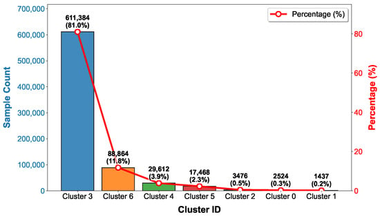
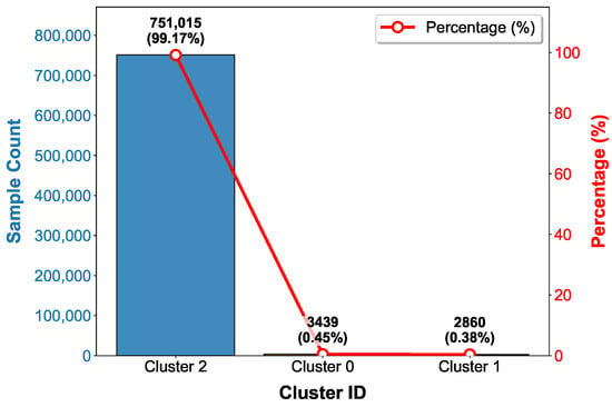
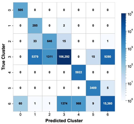
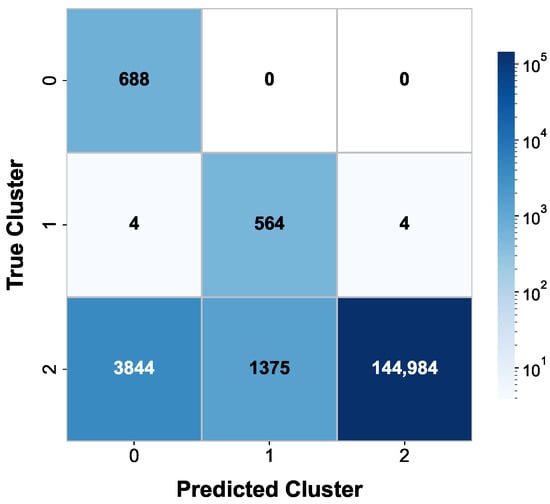
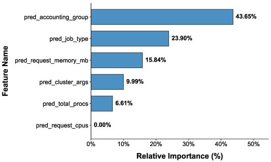
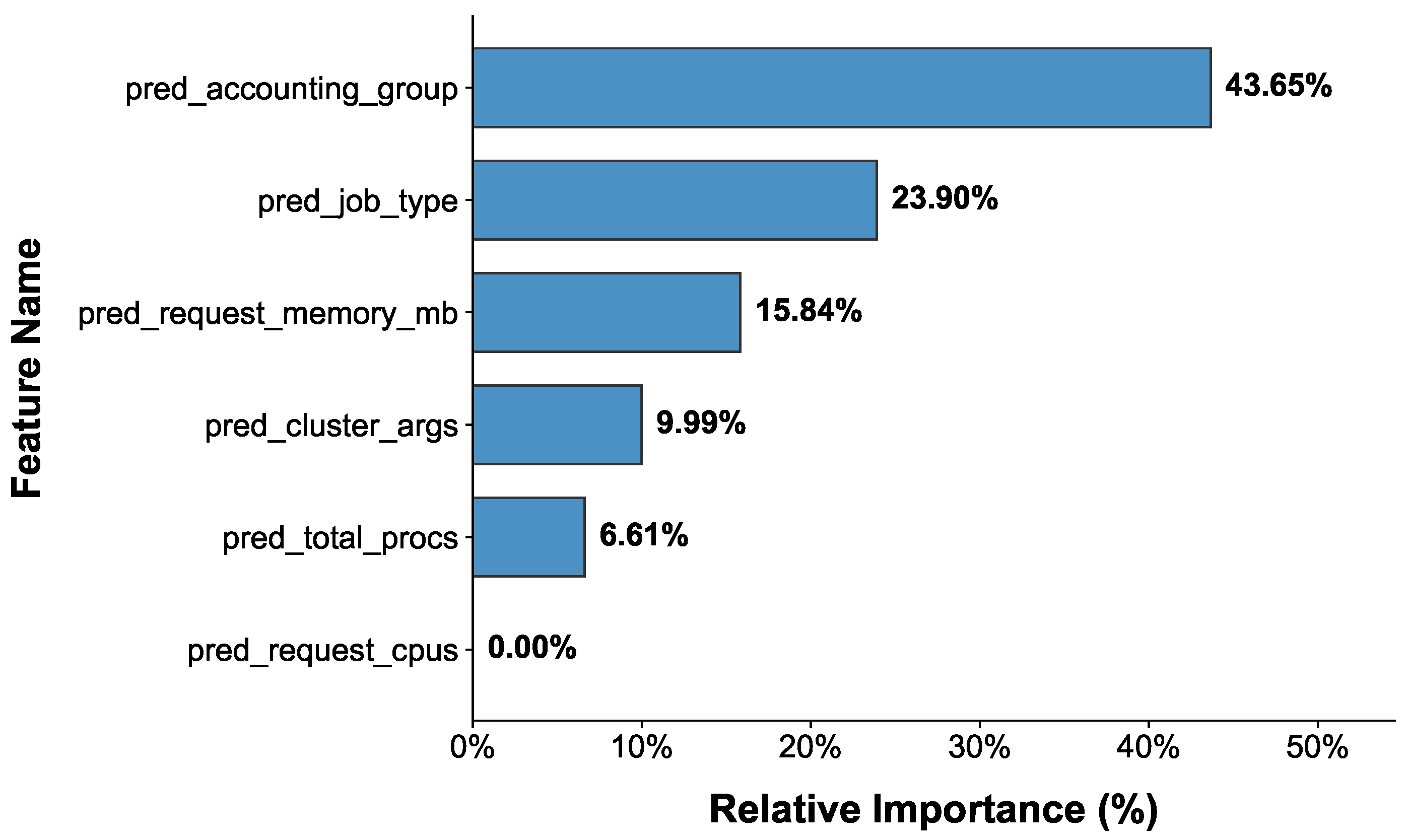
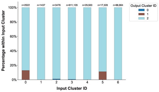
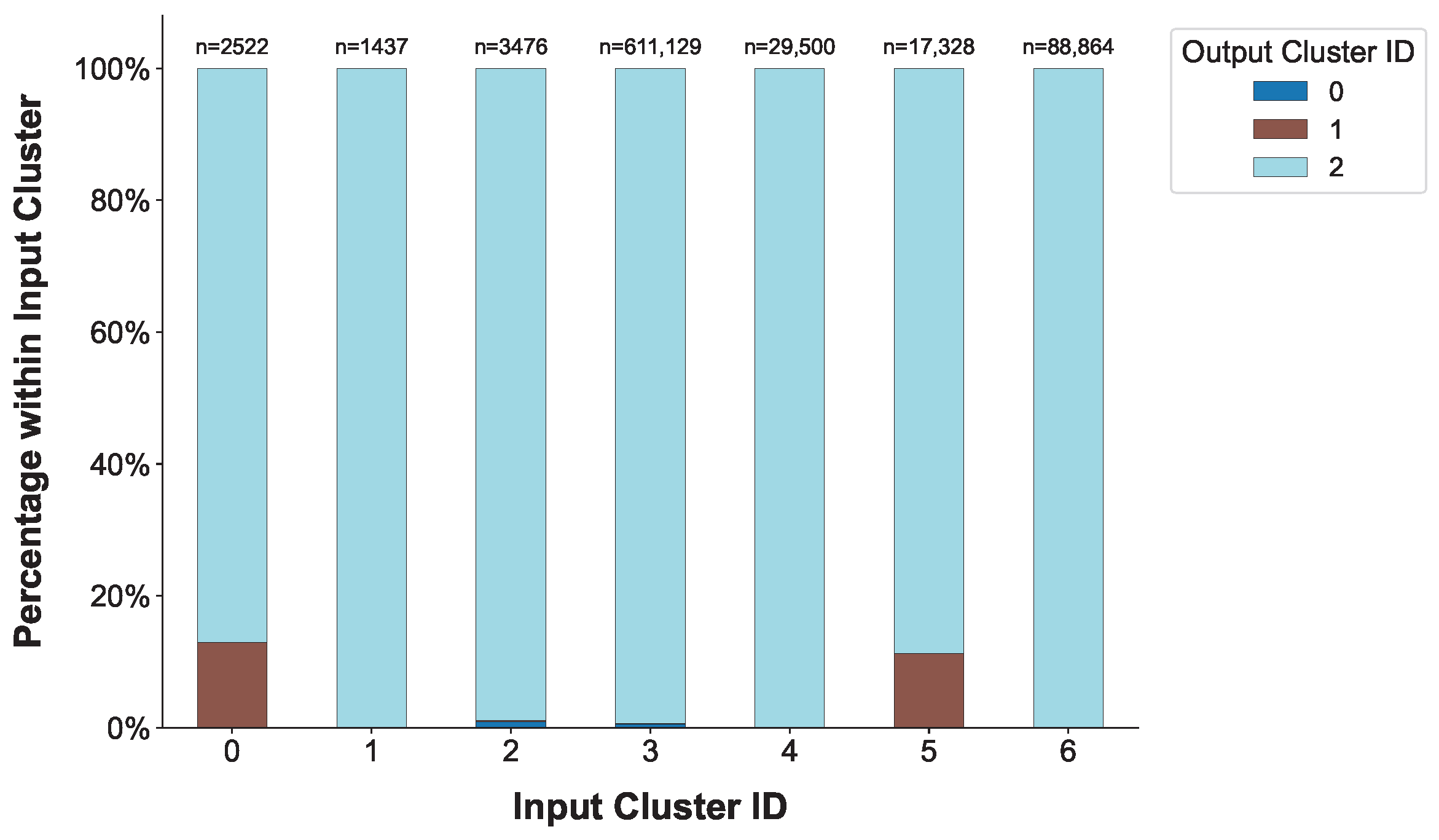

Disclaimer/Publisher’s Note: The statements, opinions and data contained in all publications are solely those of the individual author(s) and contributor(s) and not of MDPI and/or the editor(s). MDPI and/or the editor(s) disclaim responsibility for any injury to people or property resulting from any ideas, methods, instructions or products referred to in the content. |
© 2026 by the authors. Licensee MDPI, Basel, Switzerland. This article is an open access article distributed under the terms and conditions of the Creative Commons Attribution (CC BY) license.