Censoring-Aware Time-to-Success Potential Shaping for Sparse-Reward Reinforcement Learning

Abstract

Sparse rewards remain a major obstacle to efficient reinforcement learning (RL), particularly in long-horizon goal-reaching tasks where little feedback is available before successful termination. This difficulty is further complicated by time-limited trajectories, for which the absence of observed success indicates incomplete follow-up rather than necessarily a failed attempt. Existing progress-based shaping methods generally do not explicitly model this distinction, which can bias temporal progress estimates and weaken the resulting shaping signal. To address this issue, we propose Censoring-Aware Time-to-Success Potential Shaping (CTPS), a reward-shaping method that treats successful trajectories as observed time-to-event data and time-limited trajectories as right-censored data. CTPS fits a discrete hazard model to estimate the conditional time-to-success distribution, summarizes the resulting survival curve using the restricted mean time-to-success, and converts this estimate into a bounded potential. The learned temporal signal is then incorporated through a potential-based reward difference, with the potential held fixed during each target-update interval. Experiments show that CTPS reduces RMST estimation error by approximately 93% relative to timeout-as-event estimation under heavy censoring, while improving sparse-maze success rates by approximately 157% over NaiveTTS-PBRS. It also preserves state-ranking correlations above 0.98 under the evaluated behavior-policy shifts. These results characterize the temporal-estimation performance of CTPS and its use as a shaping signal in the evaluated sparse-reward tasks.

1. Introduction

Reinforcement learning (RL) has been widely adopted as a general framework for sequential decision making because policies can be optimized directly from interaction rather than from a complete analytical model of the environment [1]. Its practical efficiency, however, is often limited when informative rewards are sparse. In long-horizon goal-directed tasks, a nonzero reward may be observed only after a long sequence of decisions has been completed, so exploration and temporal credit assignment must be performed with little intermediate feedback. This difficulty has been documented in sparse-reward manipulation, navigation, and goal-reaching settings, for which goal relabeling, intrinsic motivation, and auxiliary-task control have been developed to make otherwise uninformative experience more useful [2,3,4]. More recent intrinsic-reward methods have further improved exploration by adaptively combining multiple predictive models or by learning stronger visual novelty representations [5,6]. Although these methods can improve state-space coverage, the auxiliary signal is generally designed around novelty, relabeled goals, or visitation statistics rather than around an explicit estimate of how much time remains before task success.

A complementary line of work has therefore been developed around reward shaping, in which additional feedback is supplied so that progress can be distinguished before a terminal reward is observed. The theoretical foundation was established by potential-based reward shaping (PBRS), where a shaping reward of the form $\gamma \Phi \left(s^{\prime }\right)-\Phi \left(s\right)$ was shown to preserve the optimal policy for a fixed potential [7]. The relation between PBRS and value initialization was subsequently characterized [8], and shaping potentials were shown to be learnable online rather than being restricted to manually specified heuristics [9]. Extensions were also derived for dynamically changing potentials, clarifying how policy invariance can be retained when automatically generated shaping information evolves during learning [10]. These classical results have motivated a broad family of modern learned-shaping methods. Success statistics have been used to construct self-adaptive shaping signals [11]; novelty and state significance have been combined to balance exploration and exploitation [12]; incomplete symbolic plans have been converted into robust shaping potentials for long-sequence tasks [13]; and large language models have been used to infer task progress and construct dense feedback [14]. Occupancy Reward Shaping has more recently extracted goal-reaching geometry from learned future-state occupancy distributions and exposed that geometry through a policy-preserving shaping construction [15]. Taken together, this literature shows that learned progress information can accelerate sparse-reward learning, but the usefulness of the result depends on what temporal structure is represented and on how the learned signal is coupled to the original reward.

Related progress has been made in goal-conditioned representation learning. Universal value function approximators were introduced to generalize value estimates jointly over states and goals [16], while contrastive RL was later used to learn representations whose similarity structure corresponds to goal-conditioned values [17]. Quasimetric reinforcement learning further exploited the asymmetric geometry of optimal goal-reaching values to improve sample efficiency in goal-reaching tasks [18]. These approaches make goal-reaching structure more explicit than a binary terminal label, but they do not by themselves resolve how trajectories terminated by a data-collection horizon should contribute to a learned time-to-success signal. In particular, a trajectory that has not reached the goal before a fixed cutoff contains information about elapsed or remaining time even though the eventual event time has not been observed.

The treatment of such boundaries has been recognized as important in RL. Time-limit terminations were formally distinguished from genuine environment terminations by Pardo et al., who showed that inappropriate handling of artificial time limits can create state aliasing, invalidate replayed transitions, and degrade learning [19]. From a time-to-event perspective, the same boundary has an additional statistical interpretation. If success has not been observed before data collection stops, the event time is not known; only a lower bound is available. This is the classical right-censoring setting studied by Kaplan and Meier [20] and by Cox through hazard-based regression [21]. Modern machine learning survival analysis has retained this event/censor distinction while allowing nonlinear predictors to be learned from censored observations [22]. In particular, discrete-time neural survival models can be trained directly from follow-up times and event indicators through likelihood-based objectives [23]. A bounded summary of a survival curve is provided by the restricted mean survival time (RMST), which corresponds to the expected event time truncated at a predefined horizon and can be computed as the area under the survival curve up to that horizon [24].

Survival information has recently begun to be used inside RL. Hazard estimates derived from survival models have been used as intermediate rewards for offline decision making in a medical application [25]. However, several limitations remain when this idea is considered specifically as a general reward-shaping interface for sparse-reward control. First, episode-level success scores, novelty bonuses, and other trajectory-level proxies can collapse temporal distinctions between states that occur at very different distances from the goal. Second, if every timeout is converted into a terminal failure or an observed event time, the information “success was not observed yet” is replaced by a stronger and generally unsupported label; the resulting remaining-time estimate can therefore be biased when administrative truncation is common. Third, a progress estimate used directly as a reward can become an alternative optimization objective. Proxy-reward misalignment and reward hacking have been studied explicitly in recent RL work [26,27], and the Progress Reward Model for Reinforcement Learning via Large Language Models (PRM4RL) reports that direct use of a progress score can yield high shaped return while degrading task success, whereas a potential-based construction is more stable [14]. Finally, when a learned potential is updated together with the policy, reward non-stationarity must be controlled rather than being ignored. Thus, in the literature reviewed above, the joint requirement that temporal progress be estimated from censored sparse-reward trajectories and then supplied to an arbitrary RL backbone without replacing the environment objective remains insufficiently addressed.

The central question addressed in this work is therefore whether time-to-success information can be learned from both successful and time-limited trajectories without mislabeling censored episodes, while still being used as dense feedback through an objective-preserving shaping interface. To address this question, Censoring-Aware Time-to-Success Potential Shaping (CTPS) is proposed. Each state occurrence in a successful trajectory is represented by an observed remaining time to first success, whereas each occurrence in a time-limited unsuccessful trajectory is represented by a right-censored lower bound. A discrete hazard model is fitted jointly to these observations, and the resulting survival function is summarized by an RMST estimate. The negative normalized RMST is then used as a bounded potential. Rather than being rewarded directly, this potential is exposed to the controller only through a PBRS temporal difference. A delayed copy of the survival model is kept fixed during each policy-update block so that the standard fixed-potential PBRS invariance argument applies within that block. In this way, censoring-aware temporal estimation is separated from policy optimization, while the backbone RL algorithm and the original environment reward are left unchanged.

The contributions of this work are summarized as follows:

(1)

A censoring-aware RMST potential is constructed from a discrete time-to-success survival model and incorporated into the original reward through a blockwise-frozen PBRS interface.

(2)

The proposed design is evaluated through controlled and PPO experiments, where improved temporal estimation and sparse-reward learning efficiency are demonstrated.

2. Problem Formulation

An episodic Markov decision process (MDP) is considered:

$$\mathcal{M}=(\mathcal{S},\mathcal{A},P,r^{\mathrm{env}},\gamma ,H),$$

(1)

where $\mathcal{S}$ and $\mathcal{A}$ are the state and action spaces, $P(s^{\prime }\mid s,a)$ is the transition kernel, $r^{\mathrm{env}}$ is the environment reward, $\gamma \in [0,1)$ is the discount factor, and H is the maximum episode horizon. A policy $\pi (a\mid s,g)$ may additionally condition on a goal or task descriptor g. The goal variable can be omitted in single-task environments; it is retained here for compatibility with multi-goal tasks.

Let $G_g\subseteq \mathcal{S}$ denote the set of states satisfying task g. Starting from a state occurrence $s_t$, define the first time that the trajectory reaches the success set as

$$T_g^{{\pi }_b}\left(s_t\right)=inf\{k\ge 1:s_{t+k}\in G_g\}.$$

(2)

Here, ${\pi }_b$ denotes the behavior policy that generates the trajectory data. The notation $T_g^{{\pi }_b}\left(s_t\right)$ emphasizes that time-to-success is not an intrinsic property of the state, but a policy-dependent random variable conditioned on the data-generating policy. $T_g^{{\pi }_b}\left(s_t\right)$ is therefore a random variable, since stochastic dynamics and stochastic policies can produce different success times from the same state. For a state occurrence $s_t$ in an episode, let $C_t$ denote the remaining observation window imposed by data collection. The observation is written as

$$Y_t=min(T_g^{{\pi }_b}\left(s_t\right),C_t),{\delta }_t=\mathbb{I}[T_g^{{\pi }_b}\left(s_t\right)\le C_t].$$

(3)

Let $y_t$ denote the realized value of $Y_t$. If the episode succeeds for the first time at step $t^{★}$, then $y_t=t^{★}-t$ and ${\delta }_t=1$. If the episode reaches a time limit L without success, then $y_t=L-t$, ${\delta }_t=0$, and the correct statement is $T_g^{{\pi }_b}\left(s_t\right)>y_t$. The latter is a right-censored observation rather than an observed failure time [20,22].

This paper targets tasks that terminate upon success and whose non-successful episodes end through an administrative time limit. Genuine absorbing failures, such as a collision that makes future success impossible, are not treated as censored samples. Such events require either a separate failure terminal state or a competing-risk extension. This distinction prevents the method from relabeling known catastrophic outcomes as mere missing data.

The goal is to learn a shaping function from a dataset

$${\mathcal{D}}_{\mathrm{surv}}={\left\{(s_i,g_i,y_i,{\delta }_i)\right\}}_{i=1}^N$$

(4)

without replacing the original task reward. Instead of learning an alternative reward objective, a potential $\Phi (s,g)$ is sought to summarize expected temporal progress and produce a shaped reward

$$r_t^{\mathrm{sh}}=r_t^{\mathrm{env}}+\beta \left[\gamma \Phi (s_{t+1},g)-\Phi (s_t,g)\right],$$

(5)

where $\beta \ge 0$ controls the shaping strength.

3. Methodology

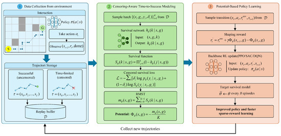
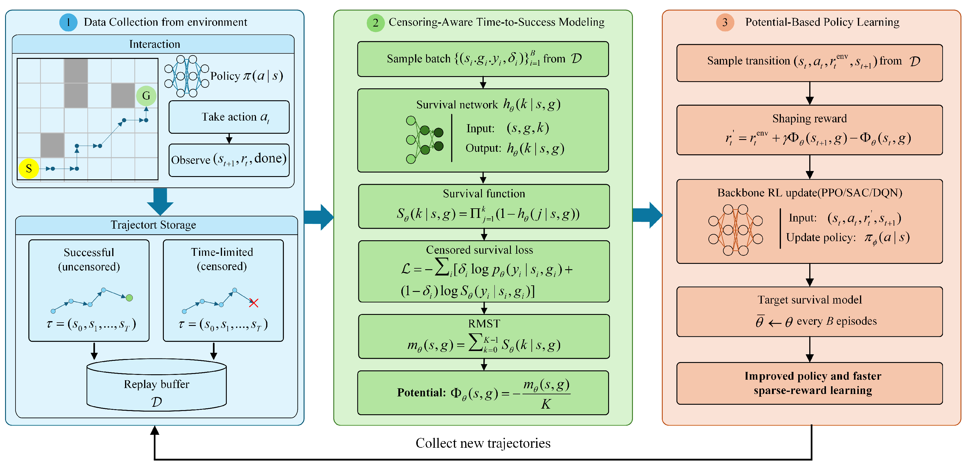
CTPS separates temporal estimation from policy optimization. Successful and time-limited state occurrences are converted into observed and right-censored time-to-success samples, respectively. A discrete hazard model is fitted to these samples, its survival distribution is summarized by the RMST, and the negative normalized RMST is used as a potential. A delayed copy of the survival model is held fixed during each policy-update block. Figure 1 summarizes this pipeline.

Figure 1. Overview of CTPS. Successful state occurrences provide observed remaining times to first success, whereas time-limit truncations provide right-censored lower bounds. A discrete hazard model estimates the conditional time-to-success distribution. Its survival function is summarized by the restricted mean time-to-success, which is converted into a bounded potential. A delayed target survival model is kept fixed during each policy-update block, and the resulting potential is supplied to the backbone RL algorithm only through a potential-based shaping difference.

3.1. Censoring-Aware Time-to-Success Estimation

CTPS estimates the random remaining time to first success under the behavior policy ${\pi }_b$ that generates the survival-training data. The resulting survival distribution is policy-conditioned rather than an intrinsic, policy-independent property of the environment; when trajectories from multiple policies are pooled, it represents the empirical mixture induced by those policies.

Using the observation pair defined in Equation (3), ${\delta }_t=1$ indicates that first success is observed and ${\delta }_t=0$ indicates right censoring. The time index counts transitions after the state occurrence: $T_g^{{\pi }_b}\left(s_t\right)=1$ means that the next transition reaches the goal. Thus, a state immediately preceding the goal has an observed remaining time of one step.

Suppose that an episode reaches the success set for the first time at step $t^{★}$. For every selected state occurrence $s_t$ before first success, the remaining event time is known exactly. The corresponding survival sample is therefore

$$y_t=t^{★}-t,{\delta }_t=1.$$

(6)

Thus, different positions in a successful trajectory receive different temporal observations.

Suppose instead that data collection terminates at step L before the goal is reached. For a state occurrence $s_t$, the available follow-up duration is $L-t$. The corresponding sample is

$$y_t=L-t,{\delta }_t=0.$$

(7)

The observation states

$$T_g^{{\pi }_b}\left(s_t\right)>y_t,$$

(8)

rather than $T_g^{{\pi }_b}\left(s_t\right)=y_t$.

These samples are collected in the survival-training dataset ${\mathcal{D}}_{\mathrm{surv}}$ defined in Section 2. For the survival window K, which specifies both the maximum modeled follow-up time and the number of discrete hazard bins, follow-up is restricted to at most K interaction steps. An event contributes ${\delta }_i=1$ only when first success is observed within this window. If success is not observed before the modeled window ends, the corresponding sample is treated as censored at K. This convention allows the survival estimator to use a fixed number of temporal bins even when the environment horizon H is larger than K.

The conversion is intended for administrative censoring. Known irreversible failures are represented separately as terminal failures rather than as censored observations. In Algorithm 1, a successful episode contributes observed events, a non-successful administrative cutoff contributes right-censored samples, and a genuine irreversible failure is recorded as a distinct terminal outcome and excluded from the success-event censoring likelihood.

Algorithm 1 Censoring-Aware Time-to-Success Potential Shaping (CTPS)

Require: RL agent $\pi$, survival model $h_{\theta }$, window K, shaping scale $\beta$, refresh interval B 1: if burn-in enabled then 2:       Collect burn-in trajectories with environment reward only; fit $h_{\theta }$ from completed episodes 3: end if 4: Initialize target parameters $\overline{\theta }\leftarrow \theta$ 5: for each episode $e=1,2,\dots$ do 6:       Roll out $\pi$; store transitions and state occurrences, using     $r_t^{\mathrm{sh}}=r_t^{\mathrm{env}}+\beta [\gamma {\Phi }_{\overline{\theta }}(s_{t+1},g)-{\Phi }_{\overline{\theta }}(s_t,g)]$ 7:       if episode succeeds at $t^{★}$ then 8:             Add observed event samples $(s_t,g,t^{★}-t,1)$ for pre-success occurrences within K 9:       else if episode ends at an administrative time limit L then 10:           Add right-censored samples $(s_t,g,min\{L-t,K\},0)$ for observed occurrences 11:     else 12:           Record irreversible failure separately; do not treat it as censoring 13:     end if 14:     Update $h_{\theta }$ with ${\mathcal{L}}_{\mathrm{surv}}$ and update $\pi$ with its standard RL rule 15:     if $emodB=0$ then 16:           $\overline{\theta }\leftarrow \theta$ 17:     end if 18: end for

Because reinforcement-learning interaction is naturally indexed by discrete environment steps, CTPS represents the event-time distribution through a discrete hazard model. For $k\in \{1,\dots ,K\}$, the hazard is defined as

$$h_{\theta }(k\mid s,g)={\mathbb{P}}_{\theta }\left(T_g^{{\pi }_b}\left(s\right)=k\mid T_g^{{\pi }_b}\left(s\right)\ge k,s,g\right),$$

(9)

where $\theta$ denotes the parameters of the survival model.

In continuous or visual state spaces, $h_{\theta }$ can be implemented by a neural state encoder followed by K sigmoid logits; in tabular environments, it can be estimated for each state.

The hazard probabilities determine the corresponding survival function,

$$S_{\theta }(k\mid s,g)={\mathbb{P}}_{\theta }(T_g^{{\pi }_b}\left(s\right)>k\mid s,g)={\displaystyle \prod _{j=1}^k}\left[1-h_{\theta }(j\mid s,g)\right],$$

(10)

with

$$S_{\theta }(0\mid s,g)=1.$$

(11)

Because P is already used for the transition kernel of the MDP, the probability mass of first success at step k is denoted by $f_{\theta }$:

$$f_{\theta }(k\mid s,g)=h_{\theta }(k\mid s,g)S_{\theta }(k-1\mid s,g).$$

(12)

For an observed event the likelihood contribution is $f_{\theta }(y_i\mid s_i,g_i)$, whereas for a censored observation it is $S_{\theta }(y_i\mid s_i,g_i)$. The resulting negative log-likelihood is

$$\begin{array}{cc}\hfill {\mathcal{L}}_{\mathrm{surv}}\left(\theta \right)=-{\displaystyle \frac{1}{N}}{\displaystyle \sum _{i=1}^N}& [{\delta }_{i}log{f}_{\theta }(y_i\mid s_i,g_i)\hfill \\ \hfill & +(1-{\delta }_i)log{S}_{\theta }(y_i\mid s_i,g_i)].\hfill \end{array}$$

(13)

Equivalently, the likelihood can be written in terms of the discrete hazards:

$$\begin{array}{cc}\hfill log{\ell }_i\left(\theta \right)=& {\delta }_i\left[log{h}_{\theta }(y_i\mid s_i,g_i)+{\displaystyle \sum _{k=1}^{y_i-1}}log\left(1-h_{\theta }(k\mid s_i,g_i)\right)\right]\hfill \\ & +(1-{\delta }_i){\displaystyle \sum _{k=1}^{y_i}}log\left(1-h_{\theta }(k\mid s_i,g_i)\right).\hfill \end{array}$$

(14)

At a censoring boundary, no positive event target is created; replacing ${\delta }_i=0$ with ${\delta }_i=1$ instead places probability mass at the timeout step. State occurrences from the same trajectory are treated as supervision pairs rather than independent physical experiments. The validity of the censoring likelihood assumes that the administrative cutoff mechanism is non-informative with respect to the unobserved event time conditional on the recorded state and follow-up. In the chain stress test, early observation is assigned by a randomized episode-level cutoff mechanism, independent of the realized transition path, while the other episodes are followed through the modeled window. State- or outcome-dependent censoring is not evaluated in the present experiments.

3.2. Survival Potential and Policy-Invariant Reward Shaping

The estimated survival distribution is compressed into a scalar potential using the RMST. In the present setting, this quantity represents the restricted mean time to success over the modeled window K:

$$m_{\theta }(s,g)={\mathbb{E}}_{\theta }\left[min\{T_g^{{\pi }_b}\left(s\right),K\}\mid s,g\right].$$

(15)

For the discrete survival representation, this quantity can be computed directly as

$$m_{\theta }(s,g)={\displaystyle \sum _{k=0}^{K-1}}{S}_{\theta }(k\mid s,g).$$

(16)

The shaping potential is defined as

$${\Phi }_{\theta }(s,g)=-{\displaystyle \frac{m_{\theta }(s,g)}{K}}.$$

(17)

For nonterminal states,

$${\Phi }_{\theta }(s,g)\in [-1,0].$$

(18)

The normalization confines the potential to $[-1,0]$ and makes its scale comparable across survival windows.

At an absorbing terminal state, the potential used by the shaping mechanism is defined to be zero:

$${\Phi }_{\theta }(s_{\mathrm{term}},g)=0.$$

(19)

The zero-terminal convention in Equation (19) is used for genuine absorbing terminations of the RL problem, including task success and any true terminal failure. An administrative time limit is handled as a truncation rather than as an absorbing terminal state: it produces a right-censored observation in ${\mathcal{D}}_{\mathrm{surv}}$, while the RL backbone retains the successor state for bootstrapping and the shaping term uses its ordinary nonterminal potential ${\Phi }_{\theta }(s_{t+1},g)$. If a finite horizon is itself part of the task definition, the horizon boundary is treated as a genuine terminal transition and the zero-terminal convention applies. Thus, the survival label and the RL termination/bootstrapping rule are determined by the semantic type of the boundary, consistently distinguishing administrative truncation from genuine termination [19].

The learned score is used exclusively through a potential difference. Let $\overline{\theta }$ denote the parameters of a delayed survival model that is held fixed during a block of policy updates. The shaping term is

$$F_t=\gamma {\Phi }_{\overline{\theta }}(s_{t+1},g)-{\Phi }_{\overline{\theta }}(s_t,g),$$

(20)

and the reward supplied to the RL backbone is

$$r_t^{\mathrm{sh}}=r_t^{\mathrm{env}}+\beta F_t,\beta \ge 0,$$

(21)

where $\beta$ controls the strength of shaping.

The coefficient $\beta$ controls shaping strength and is distinct from PPO’s generalized advantage estimation (GAE) parameter ${\lambda }_{\mathrm{GAE}}$. The shaping term is a temporal difference of the potential; for a self-loop it equals $(\gamma -1)\Phi (s,g)$ and need not be zero. Policy preservation follows from the discounted sum of shaping terms over a trajectory under the terminal conditions below, rather than from an assumption that each repeated visit contributes no reward.

For a trajectory terminating at step $\tau$, the discounted sum of shaping terms telescopes:

$$\begin{array}{ccc}\hfill {\displaystyle \sum _{t=0}^{\tau -1}}{\gamma }^t\beta F_t& =& \beta {\displaystyle \sum _{t=0}^{\tau -1}}{\gamma }^t\left[\gamma {\Phi }_{\overline{\theta }}(s_{t+1},g)-{\Phi }_{\overline{\theta }}(s_t,g)\right]\hfill \\ & =& -\beta {\Phi }_{\overline{\theta }}(s_0,g)+\beta {\gamma }^{\tau }{\Phi }_{\overline{\theta }}(s_{\tau },g).\hfill \end{array}$$

(22)

Under the terminal convention in Equation (19),

$${\Phi }_{\overline{\theta }}(s_{\tau },g)=0,$$

(23)

and hence,

$${\displaystyle \sum _{t=0}^{\tau -1}}{\gamma }^t\beta F_t=-\beta {\Phi }_{\overline{\theta }}(s_0,g).$$

(24)

For trajectories beginning from the same state and goal, the additional discounted return is therefore independent of the subsequent action sequence. The ordering of policies induced by the environment return is unchanged. Consequently, for a fixed target potential, the shaped and unshaped MDPs share the same set of optimal policies under the standard PBRS conditions [7].

The policy-invariance result above is a fixed-potential result. During adaptive training, the target potential is refreshed between update blocks to limit reward non-stationarity. This schedule does not by itself establish global policy invariance for the complete adaptive learning process; the experiments evaluate its empirical learning behavior.

3.3. Training Procedure

During online training, the survival model is updated from completed trajectories, while the potential used by the RL backbone is refreshed periodically. The target parameters $\overline{\theta }$ are copied from the online parameters $\theta$ every B episodes:

$$\overline{\theta }\leftarrow \theta \mathrm{every}B\mathrm{episodes}.$$

(25)

The interval B controls how often the target potential is refreshed and therefore the duration for which the shaping signal is held fixed. The fixed-potential invariance statement applies while a particular target snapshot is used; periodic refresh does not establish global invariance for the full adaptive procedure.

At each episode, the frozen target model is used to compute the shaping reward. After termination, state occurrences are converted into observed-event or censored samples, added to ${\mathcal{D}}_{\mathrm{surv}}$, and used to update $\theta$; the backbone agent is updated by its ordinary learning rule.

The RL component is kept algorithm-independent. For an off-policy method, ${\mathcal{D}}_{\mathrm{RL}}$ may correspond to a persistent replay buffer. For an on-policy method such as PPO, it may represent only the current rollout batch and need not persist across policy updates. Only the reward supplied to the backbone is changed; no new Bellman operator, critic architecture, or policy objective is required.

Algorithm 1 summarizes the training procedure, including optional burn-in with environment reward only until the survival model is fitted.

Three hyperparameters are used. The window K sets the modeled time range and the number of hazard outputs. The coefficient $\beta$ sets the magnitude of the shaping term relative to the environment reward. The interval B controls the trade-off between target stability and adaptation to new trajectory data. CTPS is therefore implemented as a side model: temporal structure is extracted by the survival component, converted to a bounded potential by RMST, and supplied to the unchanged RL backbone through PBRS.

4. Experiment

The experiments are organized around four aspects of CTPS: temporal ordering, RMST estimation under administrative censoring, downstream sparse-reward control, and evaluation under changes in the behavior-data distribution. A stochastic chain, an $8\times 8$ sparse maze, and MiniGrid-DoorKey-5 × 5 are used to provide progressively richer evaluation settings.

4.1. Environment

Stochastic chain: A 15-state stochastic chain with goal state 14 is used for temporal ordering and censoring analyses. For temporal ordering, trajectories are followed until success, subject to a 1000-step numerical cap. For each non-goal initial state, 1500 trajectories are used for estimation and 12,000 independent trajectories are used as the reference; $K=60$. For the censoring analysis, 20,000 complete trajectories per initial state provide the Monte Carlo RMST reference, and 1200 training trajectories per state are generated for each censoring condition. Administrative censoring is imposed after one transition with a calibrated probability; otherwise, the trajectory is followed through the $K=60$ window.

Sparse maze: The $8\times 8$ maze is used to evaluate fixed-potential control and behavior-dataset sensitivity. Episodes have horizon 60, a reward of one on goal attainment, and a 0.04 action-replacement probability. The layout contains vertical obstacle columns at $x\in \{2,4,6\}$ with openings at $y\in \{1,6,2\}$, respectively; the start and goal states are $(0,0)$ and $(7,7)$. The principal behavior dataset contains 700 trajectories generated with goal-directed action probability 0.38 and uniform action selection otherwise. Learned potentials are fitted from this dataset and held fixed during the Q-learning comparisons. Tabular Q-learning is run for 600 episodes over seeds 0–19 with $\gamma =0.99$, $\alpha =0.22$, and the episode-dependent exploration schedule

$${ϵ}_e=max\left(0.04,0.95\times {0.994}^e\right),$$

(26)

$K=60$ and $\beta =4.0$. Behavior-dataset sensitivity is evaluated with 100, 300, 700, and 1500 trajectories. The independent survival evaluation uses 700 training trajectories with $p_{\mathrm{goal}}=0.38$ and ten train/test splits with test policies defined by $p_{\mathrm{goal}}\in \{0.20,0.38,0.60\}$.

MiniGrid-DoorKey: The standard MiniGrid-DoorKey-5 × 5 task is used for PPO evaluation with its 250-step horizon and environment reward. The survival model receives a symbolic key containing the agent position, orientation, carrying status, and grid configuration. PPO is trained for 100,000 environment interactions in eight parallel environments with seeds 0–9; deterministic evaluation is conducted every 10,000 steps on 20 episodes. CTPS-PBRS and NaiveTTS-PBRS use $K=32$, $\beta =1$, and a target refresh interval of 16 completed episodes. The Sparse baseline uses the same PPO backbone and optimization protocol without shaping. A self-adaptive success-rate shaping reference and a refresh-interval sensitivity study with $B\in \{1,8,16,32,64\}$ are also included.

The PPO policy and value networks use multilayer perceptrons (MLPs). The principal experimental hyperparameters are summarized in Table 1.

Table 1. Principal hyperparameters used in the experiments.

Symbol	Value	Meaning
H	60 (maze); 250 (MiniGrid)	Maximum environment episode horizon.
K	60 (chain and maze); 32 (MiniGrid); $\{52,56,60\}$ (maze sensitivity)	Modeled time-to-success window and number of discrete hazard bins.
$\gamma$	0.99	Discount factor used by the RL backbone and PBRS difference.
$\alpha$	0.22 (maze)	Tabular Q-learning learning rate.
${ϵ}_e$	$max(0.04,0.95·{0.994}^e)$ (maze)	Episode-dependent exploration probability for tabular Q-learning.
$\beta$	4.0 (maze); 1.0 (MiniGrid); $\{1,4,8\}$ (maze sensitivity)	Coefficient multiplying the potential-based shaping difference.
B	16 completed episodes (main MiniGrid); $\{1,8,16,32,64\}$ (sensitivity)	Interval between target-survival-model refreshes; maze potentials remain frozen.
$p_c$	Calibrated to realized censoring $\{0.50,0.60,0.75,0.90\}$; early cutoff $C=1$	Probability of imposing the common one-step administrative cutoff in the chain censoring study.
$p_{\mathrm{rand}}$	0.04	Probability that a selected maze action is replaced by a uniformly sampled action.
$p_{\mathrm{goal}}$	0.38	Goal-directed action probability in the fixed maze behavior dataset.
$n_{\mathrm{beh}}$	700 (main maze and independent survival evaluation); $\{100,300,700,1500\}$ (dataset-size study)	Number of behavior trajectories used to fit the survival potential; each dataset-size condition uses a separate behavior-data collection budget.
$p_{\mathrm{goal}}^{\mathrm{test}}$	$\{0.20,0.38,0.60\}$	Goal-directed action probabilities used for the independent survival evaluation under behavior-policy shifts.
$n_{\mathrm{rep}}$	10 (sensitivity and survival-shift studies)	Independent seeds or train/test splits used for revised analyses.
$n_{\mathrm{env}}$	8	Number of parallel MiniGrid environments used during PPO training.
$n_{\mathrm{steps}}$	256	PPO rollout length per parallel environment before optimization.
$n_{\mathrm{batch}}$	256	PPO minibatch size.
$n_{\mathrm{epoch}}$	10	Number of PPO optimization epochs per rollout batch.
${\eta }_{\mathrm{PPO}}$	$3\times {10}^{-4}$	PPO Adam learning rate.
${\lambda }_{\mathrm{GAE}}$	0.95	GAE parameter used by PPO.
$c_{\mathrm{ent}}$	0.01	PPO entropy-loss coefficient.
$d_{\mathrm{MLP}}$	$(64,64)$	Hidden-layer widths of the PPO policy and value MLPs.

4.2. Compared Methods

The compared methods share the environment, backbone learner, interaction budget, optimizer, and evaluation protocol within each task. The survival-model settings and task-specific hyperparameters are listed in Table 1.

Sparse: The original environment reward is used without an auxiliary shaping term:

$$r_t^{\mathrm{Sparse}}=r_t^{\mathrm{env}}.$$

(27)

SuccessRate-PBRS: An empirical episode-level success score $u\left(s\right)$ is used as a potential:

$${\Phi }_{\mathrm{SR}}\left(s\right)=u\left(s\right),$$

(28)

with the shaped reward given by the PBRS difference. This control retains eventual-success information without modeling the remaining time to success.

NaiveTTS-PBRS: The same trajectory records as CTPS are used, but every administrative timeout is assigned $\delta =1$ at the censoring boundary. The resulting event-time estimate is converted into a potential through the same PBRS interface, isolating the effect of the event/censor distinction.

CTPS-PBRS: The observed-event and right-censored samples are fitted with the likelihood in Equation (13). The RMST in Equation (16) is converted to

$${\Phi }_{\theta }\left(s\right)=-{\displaystyle \frac{m_{\theta }\left(s\right)}{K}},$$

(29)

which enters the controller only through Equation (20).

Oracle-PBRS: In the controlled maze, a privileged shortest-path distance $d\left(s\right)$ is used as an idealized reference:

$${\Phi }_{\mathrm{Oracle}}\left(s\right)=-{\displaystyle \frac{d\left(s\right)}{d_{max}}}.$$

(30)

This reference is diagnostic rather than data-driven. The maze potentials are fitted once from the 700-trajectory behavior dataset and remain fixed throughout Q-learning. In MiniGrid, CTPS-PBRS and NaiveTTS-PBRS use $K=32$, $\beta =1$, and a target refresh interval of 16 completed episodes; the Sparse PPO control uses the same learner without shaping. A self-adaptive success-rate shaping (SASR) run is included as an auxiliary reference.

4.3. Metrics

Four metrics are used to summarize temporal representation, survival-estimation accuracy, maze control, and MiniGrid learning efficiency.

Temporal ordering: Spearman’s rank correlation $\rho$ is computed between the estimated state ordering and the reference ordering. Monte Carlo time-to-success estimates are used in the chain, and shortest-path distance is used in the maze.

RMST estimation: Estimation error is measured by

$${\mathrm{MAE}}_{\mathrm{RMST}}={\displaystyle \frac{1}{\left|\mathcal{S}\right|}}\sum _{s\in \mathcal{S}}\left|\widehat{m}\left(s\right)-m^{★}\left(s\right)\right|,$$

(31)

where $m^{★}\left(s\right)$ is the Monte Carlo reference RMST and $\widehat{m}\left(s\right)$ is obtained from the training observations. For independent survival testing, RMST MAE and RMST RMSE are evaluated against a reference generated under the test behavior policy; $\rho$ is reported separately to distinguish ordering from absolute calibration.

Maze control: The mean success rate over 600 Q-learning episodes is

$${\overline{y}}_{\mathrm{maze}}={\displaystyle \frac{1}{600}}{\displaystyle \sum _{e=1}^{600}}{y}_e,$$

(32)

where $y_e=1$ indicates goal attainment. Final maze success is averaged over episodes 501–600.

MiniGrid learning: Deterministic success $q_j$ is recorded at $t_j=\mathrm{10,000}j$, $j=1,\dots ,10$, and normalized AUC is computed as

$${\mathrm{AUC}}_{\mathrm{MG}}={\displaystyle \frac{1}{\mathrm{100,000}}}{\displaystyle \sum _{j=1}^9}{\displaystyle \frac{q_j+q_{j+1}}{2}}(t_{j+1}-t_j).$$

(33)

No step-0 value is imputed, so integration begins at 10,000 steps while normalization uses the full 100,000-step budget. Final MiniGrid success is averaged over the 80,000–100,000-step checkpoints. Learning curves show the mean across seeds with pointwise $\pm 1.96$ standard-error bands; the maze curve uses a trailing 50-episode mean.

4.4. Results

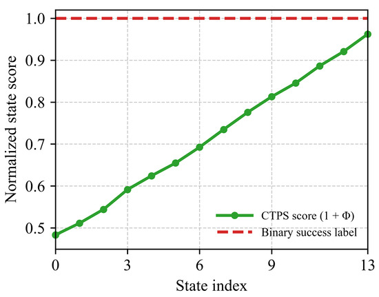
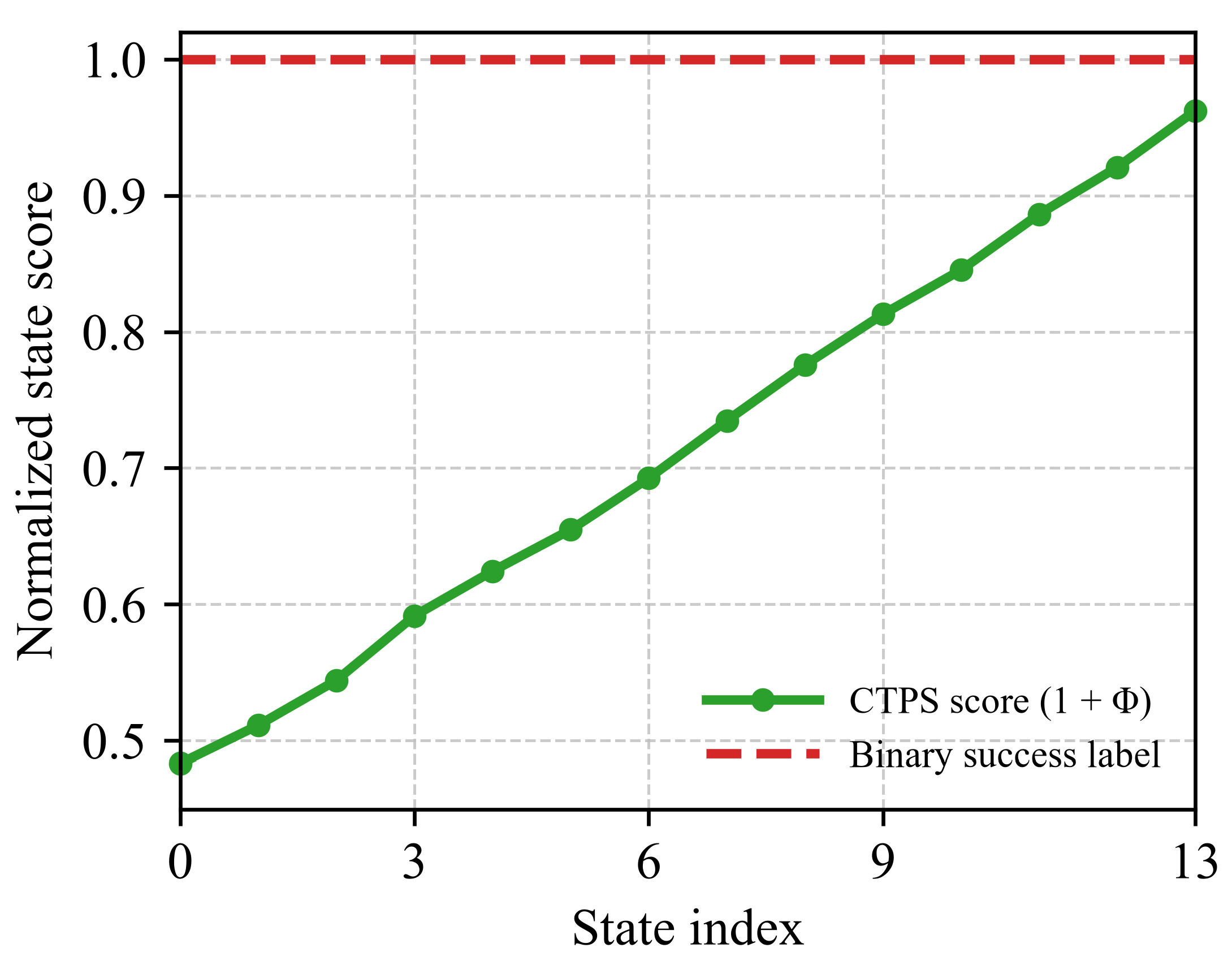
Temporal ordering is first evaluated in the stochastic chain. Because all diagnostic trajectories are followed to success, a binary episode-level label assigns the same outcome to every state occurrence despite differences in remaining time. As shown in Figure 2, the binary score collapses these temporal distinctions, whereas the CTPS potential produces 14 distinct values for the 14 non-goal states and recovers the reference ordering with Spearman correlation $\rho =1.0$.

Figure 2. Episode-level success labels collapse temporal distinctions when all trajectories eventually succeed. The time-to-success potential preserves within-trajectory ordering.

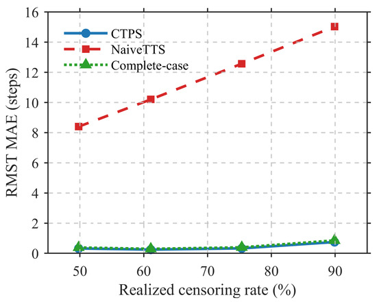
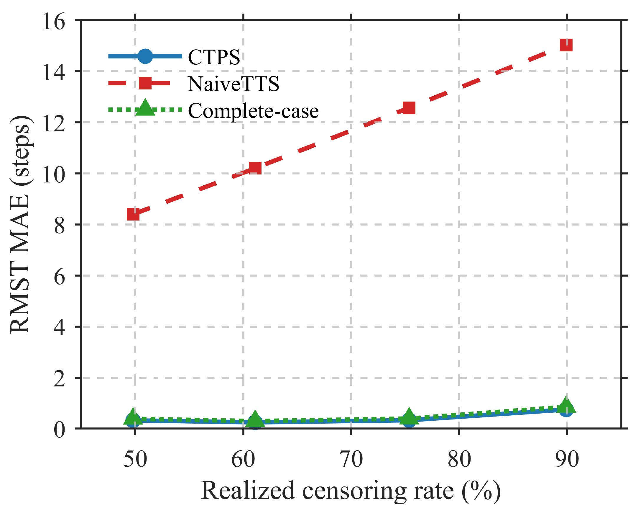
RMST estimation is then evaluated under realized censoring rates from approximately 50% to 90%. The reference RMST up to $K=60$ is obtained from 20,000 uncensored Monte Carlo trajectories per starting state, and censored datasets are generated with the common one-step-versus-full-observation protocol described in Section 4.1. Table 2 reports CTPS MAE values of 0.321, 0.244, 0.329, and 0.748 steps at 49.79%, 61.10%, 75.36%, and 89.90% censoring, respectively. The corresponding NaiveTTS MAE values are 8.400, 10.205, 12.573, and 15.035 steps, while complete-case MAE values are 0.386, 0.296, 0.395, and 0.854 steps. CTPS preserves the reference ordering with $\rho =1.000$ through 75.36% censoring and $\rho =0.996$ at 89.90%. Figure 3 plots this comparison across the four censoring levels, showing that the CTPS and complete-case errors remain below one step while the NaiveTTS error grows from 8.400 to 15.035 steps.

Table 2. RMST mean absolute error under increasing right censoring. Lower is better.

Realized Censoring	CTPS MAE	NaiveTTS MAE	Complete-Case MAE	CTPS $\mathit{\rho }$
49.79%	0.321	8.400	0.386	1.000
61.10%	0.244	10.205	0.296	1.000
75.36%	0.329	12.573	0.395	1.000
89.90%	0.748	15.035	0.854	0.996

Figure 3. RMST estimation error for CTPS, NaiveTTS, and complete-case estimation across realized censoring rates from approximately 50% to 90%.

In the sparse maze, all learned potentials are fitted from the same 700-trajectory behavior dataset and held fixed during Q-learning. The temporal-order correlations in Table 3 are 0.993 for CTPS-PBRS, 0.811 for SuccessRate-PBRS, and 0.832 for NaiveTTS-PBRS. The corresponding mean success rates over 600 control episodes are $0.548\pm 0.093$, $0.000\pm 0.000$, and $0.213\pm 0.085$; final success rates are $0.651\pm 0.109$, $0.000\pm 0.000$, and $0.250\pm 0.099$, respectively. The privileged Oracle-PBRS reference reaches $0.779\pm 0.059$ mean success and $0.900\pm 0.069$ final success.

Table 3. Sparse-maze temporal ordering and control performance over 20 seeds. Mean success rate is computed over the 600 control-training episodes; final success averages the last 100 episodes. Values are mean ± standard error, rounded to three decimal places.

Method	Temporal-Order $\mathit{\rho }$	Mean Success Rate	Final Success
Sparse	–	$0.000\pm 0.000$	$0.000\pm 0.000$
SuccessRate-PBRS	0.811	$0.000\pm 0.000$	$0.000\pm 0.000$
NaiveTTS-PBRS	0.832	$0.213\pm 0.085$	$0.250\pm 0.099$
CTPS-PBRS	0.993	$\mathbf{0.548}\pm \mathbf{0.093}$	$\mathbf{0.651}\pm \mathbf{0.109}$
Oracle-PBRS	1.000	$0.779\pm 0.059$	$0.900\pm 0.069$

The paired CTPS-minus-NaiveTTS differences are $+0.335$ for mean success rate and $+0.401$ for final success, with 95% bootstrap intervals $[0.122,0.549]$ and $[0.151,0.651]$, respectively. After Holm adjustment across the six pre-specified comparisons, the corresponding two-sided Wilcoxon p-values are 0.0156 and 0.0410 (Table 4).

Table 4. Paired significance tests for CTPS-PBRS. Differences are CTPS minus the named comparator. Confidence intervals (CIs) are paired percentile-bootstrap intervals with 20,000 resamples. Two-sided Wilcoxon signed-rank tests use matched seeds, remove zero differences, and average tied ranks; reported p-values are Holm-adjusted across the six pre-specified comparisons.

Setting	Comparator	Metric	Difference	95% CI	${\mathit{p}}_{\mathbf{Holm}}$
Sparse maze	NaiveTTS-PBRS	Mean success rate	$+0.335$	$[0.122,0.549]$	0.0156
Sparse maze	NaiveTTS-PBRS	Final success	$+0.401$	$[0.151,0.651]$	0.0410
MiniGrid DoorKey	Sparse	Success AUC	$+0.053$	$[0.017,0.092]$	0.0548
MiniGrid DoorKey	Sparse	Final success	$+0.028$	$[0.003,0.070]$	0.1250
MiniGrid DoorKey	NaiveTTS-PBRS	Success AUC	$+0.041$	$[0.012,0.072]$	0.0762
MiniGrid DoorKey	NaiveTTS-PBRS	Final success	$+0.030$	$[0.008,0.060]$	0.0762

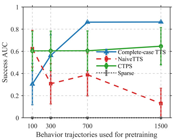
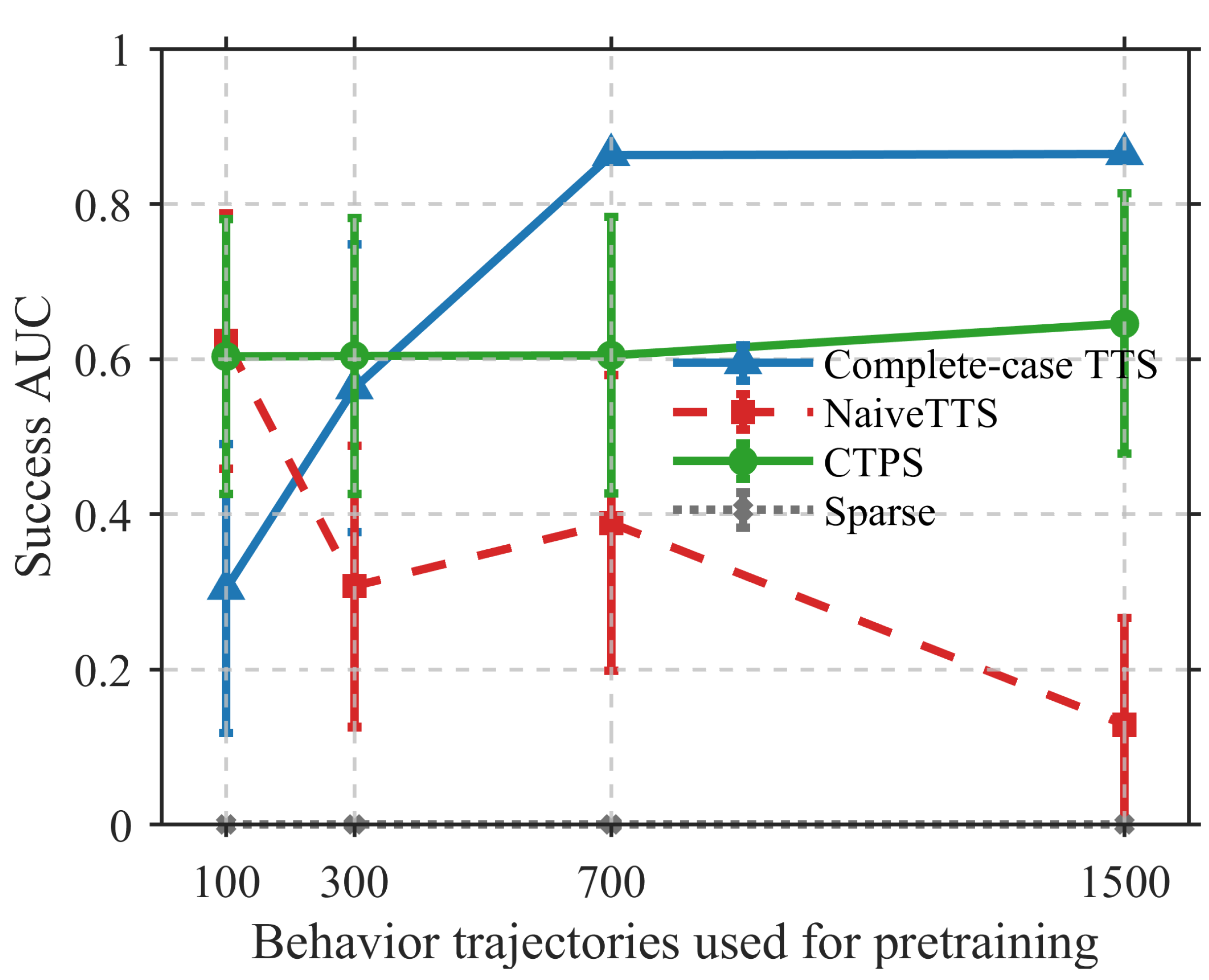
Behavior-dataset size is evaluated using prefixes of a separately collected 1500-trajectory pool at 100, 300, 700, and 1500 trajectories. The same 20 control seeds and 600-episode Q-learning budget are used at each size, with data collection additional to control training. As shown in Figure 4, CTPS-PBRS produces mean success rates of 0.603, 0.604, 0.605, and 0.646, and final success rates of 0.700, 0.699, 0.700, and 0.750, respectively.

Figure 4. Sparse-maze mean success rate across behavior-dataset sizes in a separate sensitivity analysis. Each potential is fitted from a prefix of the same 1500-trajectory behavior-data pool; each control curve uses 20 seeds and 600 Q-learning episodes. Behavior-data collection is additional to the control-training budget.

The maze sensitivity study varies $K\in \{52,56,60\}$ and $\beta \in \{1,4,8\}$ with the same 700-trajectory behavior dataset, 600 control episodes, and ten seeds. Within each K, mean success rate changes by less than 0.001 across $\beta$. The corresponding means are approximately 0.515, 0.606, and 0.605 for $K=52$, 56, and 60, respectively.

For independent survival testing, the estimator is fitted with 700 trajectories generated at $p_{\mathrm{goal}}=0.38$ and evaluated on separate 700-trajectory sets generated at $p_{\mathrm{goal}}\in \{0.20,0.38,0.60\}$. Ten independent train/test splits are used, and the reference is generated under each test policy. Table 5 reports RMST MAE values of 8.912, 1.439, and 13.032 steps, together with RMST RMSE values of 10.924, 2.505, and 13.886 steps. Spearman correlations remain between 0.982 and 0.983 across the three test policies.

Table 5. Independent survival evaluation under behavior-policy shifts. Values are mean ± standard error over ten independent train/test splits.

Test ${\mathit{p}}_{\mathbf{goal}}$	Test Success Rate	RMST MAE	RMST RMSE	Spearman $\mathit{\rho }$
0.20	$0.021\pm 0.002$	$8.912\pm 0.212$	$10.924\pm 0.215$	$0.982\pm 0.007$
0.38	$0.443\pm 0.002$	$1.439\pm 0.093$	$2.505\pm 0.195$	$0.983\pm 0.007$
0.60	$0.989\pm 0.001$	$13.032\pm 0.211$	$13.886\pm 0.184$	$0.983\pm 0.006$

MiniGrid PPO is evaluated with ten seeds, 100,000 environment interactions, eight parallel environments, and deterministic evaluation on 20 episodes every 10,000 steps. Table 6 gives normalized success AUC values of $0.592\pm 0.032$ for CTPS-PBRS, $0.551\pm 0.041$ for NaiveTTS-PBRS, and $0.539\pm 0.032$ for Sparse. Final success values are 1.000, 0.970, and 0.972, respectively. The paired AUC differences are $+0.053$ versus Sparse and $+0.041$ versus NaiveTTS-PBRS, with Holm-adjusted p-values of 0.0548 and 0.0762 (Table 4).

Table 6. MiniGrid-DoorKey-5 × 5 performance over seeds 0–9. Values are mean ± standard error. AUC uses the ten evaluation checkpoints without imputing an unobserved step-0 success value; final success averages the last three checkpoints.

Method	Success AUC	Final Success
Sparse	$0.539\pm 0.032$	$0.972\pm 0.020$
NaiveTTS-PBRS	$0.551\pm 0.041$	$0.970\pm 0.015$
CTPS-PBRS	$\mathbf{0.592}\pm \mathbf{0.032}$	$\mathbf{1.000}\pm \mathbf{0.000}$

Table 7 reports the MiniGrid sensitivity to the target-potential refresh interval B. Across the refresh-interval sweep $B\in \{1,8,16,32,64\}$, success AUC ranges from 0.5715 to 0.6018 and final success from 0.9550 to 0.9917; the Friedman test gives $p=0.7811$. The auxiliary SASR run yields AUC $0.5795\pm 0.0221$ and final success $0.9967\pm 0.0022$.

Table 7. MiniGrid sensitivity to the target-potential refresh interval B. Values are mean ± standard error over ten seeds.

B	Success AUC	Final Success
1	$0.5875\pm 0.0196$	$0.9883\pm 0.0070$
8	$0.5715\pm 0.0231$	$0.9917\pm 0.0045$
16	$0.5860\pm 0.0195$	$0.9550\pm 0.0221$
32	$0.5873\pm 0.0204$	$0.9800\pm 0.0082$
64	$0.6018\pm 0.0277$	$0.9883\pm 0.0056$

Across the three settings, CTPS preserves temporal ordering, maintains low RMST estimation error under heavy administrative censoring, and provides a stronger shaping signal than timeout-as-event estimation in the sparse maze. In MiniGrid, the principal difference appears in learning efficiency, while final success remains comparable across the main controls.

5. Conclusions

This work addresses a practical difficulty in sparse-reward reinforcement learning: trajectories that end at a time limit contain useful temporal information even when success has not yet been observed. We proposed CTPS, which represents successful state occurrences as observed time-to-success events and time-limited occurrences as right-censored observations. A discrete hazard model is used to estimate the remaining-time distribution, and its RMST is converted into a bounded potential that enters the reward only through a potential-based difference. This separates temporal estimation from the original control objective while retaining information that would be lost by treating every timeout as an observed event. The experiments show that CTPS preserves within-trajectory temporal ordering, produces substantially more accurate RMST estimates as censoring increases, and provides a more effective shaping signal than naive timeout handling. In the sparse maze, these improvements translate into markedly higher learning efficiency and final success, while the MiniGrid results show a smaller but consistent advantage during early PPO training.

The present evaluation focuses on administrative right censoring and compact goal-reaching environments, which provides a controlled setting for isolating the temporal-estimation mechanism. The MiniGrid evaluation uses a symbolic state key and does not test a learned survival model on pixel observations. Extensions to higher-dimensional observations, longer-horizon tasks, and broader policy shifts remain useful directions for future work.

References

- Sutton, R.S.; Barto, A.G. Reinforcement Learning: An Introduction, 2nd ed.; MIT Press: Cambridge, MA, USA, 2018. [Google Scholar]
- Andrychowicz, M.; Wolski, F.; Ray, A.; Schneider, J.; Fong, R.; Welinder, P.; McGrew, B.; Tobin, J.; Abbeel, P.; Zaremba, W. Hindsight Experience Replay. In Proceedings of the Advances in Neural Information Processing Systems, Long Beach, CA, USA, 4–9 December 2017; Volume 30, pp. 5048–5058. [Google Scholar]
- Pathak, D.; Agrawal, P.; Efros, A.A.; Darrell, T. Curiosity-Driven Exploration by Self-Supervised Prediction. In Proceedings of the 34th International Conference on Machine Learning; Proceedings of Machine Learning Research (PMLR): Cambridge, MA, USA, 2017; Volume 70, pp. 2778–2787. [Google Scholar]
- Riedmiller, M.; Hafner, R.; Lampe, T.; Neunert, M.; Degrave, J.; van de Wiele, T.; Mnih, V.; Heess, N.; Springenberg, J.T. Learning by Playing: Solving Sparse Reward Tasks from Scratch. In Proceedings of the 35th International Conference on Machine Learning; Proceedings of Machine Learning Research (PMLR): Cambridge, MA, USA, 2018; Volume 80, pp. 4344–4353. [Google Scholar]
- Park, G.; Jung, W.; Han, S.; Choi, S.; Sung, Y. Adaptive multi-model fusion learning for sparse-reward reinforcement learning. Neurocomputing 2025, 633, 129748. [Google Scholar] [CrossRef] [Scilit]
- Jiang, W.; Liu, G.; Leng, Q.; Guo, N. Curiosity-driven exploration based on hierarchical vision transformer for deep reinforcement learning with sparse rewards. Neurocomputing 2025, 639, 130252. [Google Scholar] [CrossRef] [Scilit]
- Ng, A.Y.; Harada, D.; Russell, S.J. Policy invariance under reward transformations: Theory and application to reward shaping. In Proceedings of the 16th International Conference on Machine Learning, Bled, Slovenia, 27–30 June 1999; pp. 278–287. [Google Scholar]
- Wiewiora, E. Potential-Based Shaping and Q-Value Initialization Are Equivalent. J. Artif. Intell. Res. 2003, 19, 205–208. [Google Scholar] [CrossRef] [Scilit]
- Grześ, M.; Kudenko, D. Online learning of shaping rewards in reinforcement learning. Neural Netw. 2010, 23, 541–550. [Google Scholar] [CrossRef] [Scilit]
- Devlin, S.M.; Kudenko, D. Dynamic Potential-Based Reward Shaping. In Proceedings of the 11th International Conference on Autonomous Agents and Multiagent Systems; IFAAMAS: Richland County, SC, USA, 2012; pp. 433–440. [Google Scholar]
- Ma, H.; Luo, Z.; Vo, T.V.; Sima, K.; Leong, T.Y. Highly Efficient Self-Adaptive Reward Shaping for Reinforcement Learning. In Proceedings of the International Conference on Learning Representations, Singapore, 24–28 April 2025. [Google Scholar]
- Ma, H.; Li, F.; Lim, J.Y.; Luo, Z.; Vo, T.V.; Leong, T.Y. Catching Two Birds with One Stone: Reward Shaping with Dual Random Networks for Balancing Exploration and Exploitation. In Proceedings of the 42nd International Conference on Machine Learning; Proceedings of Machine Learning Research (PMLR): Cambridge, MA, USA, 2025; Volume 267, pp. 41975–41991. [Google Scholar]
- Müller, H.; Berg, L.; Kudenko, D. Using Incomplete and Incorrect Plans to Shape Reinforcement Learning in Long-Sequence Sparse-Reward Tasks. Neural Comput. Appl. 2025, 37, 18851–18866. [Google Scholar] [CrossRef] [Scilit]
- Zhang, X.; Gao, N.; Jiang, X.; Chen, Y.; Pan, Y.; Zhang, M.; Deng, Y. Progress Reward Model for Reinforcement Learning via Large Language Models. In Proceedings of the Advances in Neural Information Processing Systems, San Diego, CA, USA, 2–7 December 2025; pp. 111703–111730. [Google Scholar]
- Venugopal, A.; Chen, J.; Wu, X.; Zheng, C.; Eysenbach, B.; Schneider, J. Occupancy Reward Shaping: Improving Credit Assignment for Offline Goal-Conditioned Reinforcement Learning. In Proceedings of the International Conference on Learning Representations, Rio de Janeiro, Brazil, 23–27 April 2026. [Google Scholar]
- Schaul, T.; Horgan, D.; Gregor, K.; Silver, D. Universal Value Function Approximators. In Proceedings of the 32nd International Conference on Machine Learning; Proceedings of Machine Learning Research (PMLR): Cambridge, MA, USA, 2015; Volume 37, pp. 1312–1320. [Google Scholar]
- Eysenbach, B.; Zhang, T.; Levine, S.; Salakhutdinov, R. Contrastive Learning as Goal-Conditioned Reinforcement Learning. In Proceedings of the Advances in Neural Information Processing Systems, New Orleans, LA, USA, 28 November–9 December 2022; pp. 35603–35620. [Google Scholar] [CrossRef] [Scilit]
- Wang, T.; Torralba, A.; Isola, P.; Zhang, A. Optimal Goal-Reaching Reinforcement Learning via Quasimetric Learning. In Proceedings of the 40th International Conference on Machine Learning; Proceedings of Machine Learning Research (PMLR): Cambridge, MA, USA, 2023; Volume 202, pp. 36411–36430. [Google Scholar]
- Pardo, F.; Tavakoli, A.; Levdik, V.; Kormushev, P. Time Limits in Reinforcement Learning. In Proceedings of the 35th International Conference on Machine Learning; Proceedings of Machine Learning Research (PMLR): Cambridge, MA, USA, 2018; Volume 80, pp. 4045–4054. [Google Scholar]
- Kaplan, E.L.; Meier, P. Nonparametric Estimation from Incomplete Observations. J. Am. Stat. Assoc. 1958, 53, 457–481. [Google Scholar] [CrossRef]
- Cox, D.R. Regression Models and Life-Tables. J. R. Stat. Soc. Ser. B (Methodol.) 1972, 34, 187–202. [Google Scholar] [CrossRef] [Scilit]
- Wang, P.; Li, Y.; Reddy, C.K. Machine Learning for Survival Analysis: A Survey. ACM Comput. Surv. 2019, 51, 1–36. [Google Scholar] [CrossRef] [Scilit]
- Gensheimer, M.F.; Narasimhan, B. A Scalable Discrete-Time Survival Model for Neural Networks. PeerJ 2019, 7, e6257. [Google Scholar] [CrossRef] [Scilit]
- Royston, P.; Parmar, M.K.B. Restricted Mean Survival Time: An Alternative to the Hazard Ratio for the Design and Analysis of Randomized Trials with a Time-to-Event Outcome. BMC Med. Res. Methodol. 2013, 13, 152. [Google Scholar] [CrossRef] [Scilit]
- Choi, D.H.; Lim, M.H.; Hong, K.J.; Kim, Y.G.; Park, J.H.; Song, K.J.; Shin, S.D.; Kim, S. Individualized decision making in on-scene resuscitation time for out-of-hospital cardiac arrest using reinforcement learning. npj Digit. Med. 2024, 7, 276. [Google Scholar] [CrossRef] [Scilit]
- Jiang, Z.; Feng, X.; Weng, P.; Zhu, Y.; Song, Y.; Zhou, T.; Hu, Y.; Lv, T.; Fan, C. Reinforcement Learning from Imperfect Corrective Actions and Proxy Rewards. In Proceedings of the International Conference on Learning Representations, Singapore, 24–28 April 2025. [Google Scholar]
- Liu, Z.; Sun, X.; Zheng, Z. Robust Optimization for Mitigating Reward Hacking with Correlated Proxies. In Proceedings of the International Conference on Learning Representations, Rio de Janeiro, Brazil, 23–27 April 2026. [Google Scholar]
Disclaimer/Publisher’s Note: The statements, opinions and data contained in all publications are solely those of the individual author(s) and contributor(s) and not of MDPI and/or the editor(s). MDPI and/or the editor(s) disclaim responsibility for any injury to people or property resulting from any ideas, methods, instructions or products referred to in the content. |
© 2026 by the authors. Licensee MDPI, Basel, Switzerland. This article is an open access article distributed under the terms and conditions of the Creative Commons Attribution (CC BY) license.