


Abstract
For UAVs, the industry currently relies on expensive sensors for obstacle avoidance. A significant challenge arises from the scarcity of high-quality depth estimation datasets tailored for low-altitude environments, which hinders the advancement of self-supervised learning methods in these settings. Furthermore, mainstream depth estimation models capable of achieving obstacle avoidance through image recognition are built upon convolutional neural networks or hybrid Transformers. Their high computational costs make deployment on resource-constrained edge devices challenging. While existing lightweight convolutional networks reduce parameter counts, they struggle to simultaneously capture essential features and fine details in complex scenes. In this work, we introduce LFP-Mono as a lightweight self-supervised monocular depth estimation network. In the paper, we will detail the Pooling Convolution Downsampling (PCD) module, Continuously Dilated and Weighted Convolution (CDWC) module, and Cross-level Feature Integration (CFI) module. All results show that LFP-Mono outperforms existing lightweight methods on the KITTI benchmark, and by evaluating with the Make3D dataset, show that our method generalizes outdoors. Finally, by training and testing on the Syndrone dataset, baseline work shows that LFP-Mono exceeds state-of-the-art methods for low-altitude drone performance.
1. Introduction
In low-altitude unmanned aerial vehicle (UAV) flight scenarios, obstacle avoidance strategies relying on data from expensive equipment such as LiDAR, combined with the scarcity of computational power on edge devices, highlight the importance of ensuring safe flight through low-computation and cost-effective fundamental approaches like depth estimation and object detection [1]. Estimating depth from a single image is a core and challenging task in computer vision. It is highly valuable for applications including autonomous driving, robotic navigation, and augmented reality. To address this, supervised learning methods leveraging convolutional neural networks (CNNs) have demonstrated substantial progress [2,3,4]; their development is largely constrained by the difficulty and high cost of acquiring large-scale, accurately annotated ground-truth depth data. In recent years, self-supervised training approaches that leverage geometric constraints from image sequences [5] or stereo pairs [6] have emerged as a powerful alternative, reducing reliance on expensive, accurately labeled depth data. Methods relying on unconstrained monocular video [5] offer enhanced practicality and reliability for real-world deployment by utilizing only images captured from differing camera positions for training, yet their foundational approach of view synthesis through photometric reconstruction loss minimization remains prone to performance degradation from object occlusion, camera motion, and illumination changes [7]. The comparative complexity of collecting and processing stereo image pairs has further limited their mainstream adoption, prompting the introduction of various new constraints [8,9]. In keeping with the self-supervised paradigm, this study will utilize consecutive frames from monocular video for training.
Depth data at low altitudes (for use in UAV applications) are severely lacking; whereas for example, LiDAR was provided by the KITTI ground truth dataset at ground level, a large UAV dataset with accurate depth measurements and associated point clouds are simply not available because of logistic challenges and expense associated with collecting synchronized sensor data from an aerial platform. Because of the absence of a depth dataset to train supervised models quantitatively at low altitude, models cannot be developed to operate with precision in low-altitude scenarios. Self-supervised techniques fill this gap by applying geometric constraints based on unlabeled video to enable depth estimation without reliance on an annotated depth label for training. Photometric consistency is used as an “unlabeled training signal” through geometric constraint to reduce dependence on the absence of a depth label and allow for generalization across many low-altitude environments where labeled data are lacking. As such, a self-supervised methodology is not just an alternative method but rather a necessary method for continuing to develop models capable of estimating depth within a UAV context.
Although there are advantages to using these techniques when working with UAVs flying at low altitude (e.g., 20 m), there are also some unique considerations associated with the application of these techniques to the unique characteristics of low-altitude environments. The object scales and spatial configuration within a low-altitude environment are dramatically different from the object scales and spatial configuration of an aerial photograph taken from a ground-level perspective. Therefore, the significance of some objects, such as pedestrians and vehicles, is increased as an obstacle avoidance concern when operating in a low-altitude environment. In addition, the building textures and the road outlines of objects, or the road/sidewalk outlines, require the preservation of very fine detail. Many traditional models are unable to perform well in a low-altitude environment because high computational demands inhibit their operation on UAV edge devices. Thus, a lightweight architecture that provides an appropriate balance of the preservation of detail and the understanding of context will be required for UAV operations in the low-altitude environment.
To create precise depth maps, it is essential to have a good understanding of the complexities of the scene’s structure (e.g., buildings, roads) as accurately as possible. This is very important for creating a depth map as accurately as possible. Convolutional neural networks are very effective at identifying local features and spatial relationships between those features but their small receptive fields limit their ability to model long-range dependencies and to find the global context needed for a complete understanding of the scene. To overcome this shortcoming, some researchers have created deeper or more complex CNN architectures [6,10,11]; however, these approaches typically increase the computational cost and parameter size of the network without fully solving the issue of positional modeling, resulting in the inability to accurately estimate depth as a result of an inability to determine the relationship between an object and the surrounding background. By design, Vision Transformers [12] provide global receptive fields and can use self-attention to capture the relationships between dots; however, even though self-attention enables effective modeling of relationships, the standard self-attention mechanism is quadratic in complexity with respect to input length, and therefore does not allow for lightweight models to be deployed for high-resolution imagery. Additionally, Transformers may not provide as much local detail as CNNs. Many of the current lightweight self-supervised monocular models [10] use the approach of combining CNN modules with transformer modules and lose much of the detailed information during the process of downsampling. Therefore, when high-level and low-level features interact with each other, they do not have sufficient detail of what they represent, so small or distant objects may be missed or their boundaries may be blurred together and the model may not be able to leverage cross-level features within a model for local precision and global structure within a single network to generalize across multiple use cases.
In low-altitude environments, the challenges become even worse due to the fact that faraway objects look smaller than they actually are when viewed from a distance, so long-range dependency modeling is needed. Additionally, the close-range views require detailed high-resolution data in order to detect obstacles near or around them. To overcome these limitations, we developed LFP-Mono as an architecture that utilizes lightweight design and multi-scale feature fusion techniques to optimize the way UAS can view their surroundings. For example, the PCD retains the spatial information necessary to identify small obstacles while the CDWC allows for an increased receptive field necessary to see the effects of environmental changes in aerial views.
From the previous analysis, this research article has built on the developments of Monodepth2 and Lite-Mono and developed an improved version of both of these models called LFP-Mono, which uses a lightweight design to estimate monocular depth through self-supervised learning. The new encoder-decoder design will use a new method, Pooling and Convolution Downsampling (PCD), for reducing the loss of details throughout the downsampled resolution as well as providing multi-scale spatial information. The new PCD module allows the model to keep both detailed and less detailed images when downsampling them. To further develop the model’s ability to perceive information, the new CDWC (Continuously Dilated and Weighted Convolutions) module allows the model to add additional receptive fields without increasing the kernel size by using stacked dilated convolutions that have varying dilation rates and a learnable weighting mechanism. The CDWC module allows the model to capture contextual information over multiple scales and to learn better object boundaries. To enable the model to effectively utilize both local and global information, a new CFI (Cross-level Feature Integration) module allows the model to combine the advantages of both human-vision-based spatial attention and cross-covariance-based channel attention mechanisms and provide adaptive aggregation of features across both spatial and channel dimensions. The CFI module has a new Adaptive Dual Fusion sub-module which enables it to increase the level of feature interactions through cross-gating and bilinear operations. The PoseNet is used for estimating the camera pose between different frames, and both the PoseNet and depth network are jointly optimized through the photometric reconstruction loss.
Currently, there is no clear definition of the parameter threshold for lightweight models in the market. However, most models that can be deployed on edge devices have fewer than 5M parameters and a FLOPS computation of less than 8G. Therefore, we define the standard for lightweight models as having fewer than 5M parameters and a FLOPS computation of less than 8G. LFP-Mono, with 2.0M parameters, reduces parameters by 85% compared to Monodepth2-Res50 (32.5M) [13] and by 35% compared to Lite-Mono (3.1M) [10], while maintaining competitive accuracy on the benchmark KITTI dataset.
The main contributions of this paper are summarized as follows:
- LFP-Mono is proposed as a novel lightweight network for self-supervised monocular depth estimation, balancing local detail capture with global context modeling while preserving low computational complexity.
- The PCD module is designed to mitigate spatial information loss during downsampling through combined pooling and convolutional operations, preserving multi-scale spatial details essential for accurate depth prediction of small objects.
- The CDWC module employs stacked weighted dilated convolutions to efficiently expand the receptive field, thereby enhancing perception of object boundaries, small targets, and distant regions.
- We develop a CFI module that utilizes a dual-attention mechanism to achieve comprehensive feature interaction and fusion, enabling the network to better perceive complex scene structures.
- Our model has been experimentally benchmarked and evaluated on the KITTI [14] dataset, showing that our model achieves leading performance among lightweight methods. Additional training and evaluation on the Make3D [15] and the application of our model in the UAV space has shown positive results from both the training and testing of the low-altitude Syndrone [16] dataset and from direct assessment of its performance at 20 m altitude (Section 4.5).
2. Related Works
2.1. Self-Supervised Monocular Depth Estimation
Self-supervised monocular depth estimation has gained popularity as a key area of research in computer vision. In contrast to depth map creation using stereo-pairs of images, most early models for self-supervised monocular depth estimation were developed using stereo image pairs. Garg et al. [17] were the first to frame depth estimation as view synthesis and optimize photometric consistency loss across the left and right images of stereo pairs. In addition to this work, Godard et al. introduced an additional left-right consistency constraint which significantly improved the accuracy of disparity predictions [6]; however, the constraints posed by requiring calibrated stereo pairs [6] hindered their practical applicability. To eliminate this limitation, Zhou et al. [18] developed the ground-breaking SfMLearner framework, which estimates depth maps and camera poses from monocular video sequences while also providing an explainability prediction network that deals with occlusions and dynamic objects. This work represented the first time monocular depth estimation could be performed without being supervised by stereo images, and as such served as a major catalyst for a substantial number of subsequent video self-supervised monocular depth estimation works.
A significant amount of work has been done on addressing the difficulties of occluded and independently moving objects through research that follows. Godard et al. [13] created an innovative, widely used framework called Monodepth2 based on using a minimum reprojection loss and an auto-masking strategy to remove invalid pixels, which led to a substantial increase in both robustness and accuracy from previous methods [13]. Monodepth2 has become a benchmark for future work as it provided the best performance achieved to date without needing any extra associated tasks. Additional improvements to Monodepth2 were made through utilizing a multi-frame loss strategy [13] for selecting the most reliable views for supervision, uncertainty modeling, as well as utilizing geometric consistency constraints to provide more robustness in dynamic scenes [17]. Collectively, the above advancements have increased the broader applicability of self-supervised monocular depth estimation in real-world situations.
Next to advancements in loss function structuring and occlusion handling, the use of auxiliary task types and alternate data sources has led researchers to significantly improve upon the performance of depth estimation algorithms using monocular cameras. Multi-task learning is one of many ways in which researchers have successfully integrated optical flow estimation, which estimates pixel correspondences between frames, into single-view depth estimation algorithms to increase temporal consistency of estimated depths [8]. Semantic segmentation helps researchers identify dynamic objects that may obstruct depth estimates, thus helping maintain the overall geometry of a scene [19]. Some researchers have also implemented teacher–student learning strategies that improve the accuracy of predicted depths surrounding occlusion boundaries and significant depth discontinuities [20]. Chen et al. [21] developed a novel approach to monocular depth prediction that does not depend upon traditional forms of supervision; instead, they formulated the problem of monocular depth prediction into a simple function of relative depth relationships, using the Depth-in-the-Wild dataset, and transforming it into a function-relational framework. Similarly, Gur et al. [22] used depth information inferred from the blur of motion to inform their monocular depth predictions using a convolutional layer that mimicked the point spread function. In addition to the aforementioned methods, Masoumian et al. [23] introduced the use of Graph Convolutional Networks as a means of enhancing the identification of the geometric boundaries of objects and the spatial localization of objects within complex scenes. These various lines of investigation suggest a growing recognition by researchers of the importance of integrating auxiliary knowledge, utilizing weakly supervised learning algorithms, and including structural features in order to improve the robustness and accuracy of monocular depth estimations.
2.2. Monocular Supervised Depth Estimation
In supervised monocular depth estimation, networks learn to map RGB inputs to depth values using high-quality ground-truth depth maps as supervisory signals. The model that Eigen et al. [24] developed was a multi-scale convolutional neural network that used separate branches to identify coarse and fine-grained details in a single image. Laina et al. [3] advanced the optimization of this model by creating a novel upsampling module that used the reverse Huber loss criterion. Numerous other researchers [18,25,26] have also integrated CRFs into deep models in order to enhance the performance of deep models for predicting depth by delineating semantic layer features into separate layers and developing multi-scale features using CRFs.
To alleviate instability in direct regression, Fu et al. reformulated monocular depth estimation as an ordinal regression problem, achieving superior accuracy and faster convergence [27]. Subsequent studies further extended this idea by casting depth prediction as either a classification or a hybrid classification-regression task, balancing optimization stability with precise continuous depth estimation [13].
More recently, Transformer-based models have been introduced to capture long-range dependencies and global semantic correlations [28]. Vision Transformer (ViT)-based architectures have shown the ability to model cross-region relationships, achieving significant improvement in accuracy [22,29]. A representative example is Depth Anything [30], which leverages a MiDaS teacher model with DINOv2 pre-trained weights and trains a student model on large-scale unlabeled data, demonstrating the potential of vision foundation models for monocular depth estimation [31]. Beyond static images, some studies extended monocular depth estimation to video sequences by incorporating temporal and geometric consistency constraints to stabilize inter-frame predictions [26,32].
Efficiency has also been an active research focus. Alhashim and Wonka demonstrated that high-resolution depth maps can be obtained using strong pre-trained encoders with data augmentation, even with a simple decoder [33]. Spek et al. employed knowledge distillation to design lightweight networks capable of real-time inference on embedded devices [34].
Overall, supervised monocular depth estimation has evolved considerably, from early multi-scale CNNs to ordinal regression, hybrid classification-regression frameworks, and Transformer-based architectures. These approaches have achieved remarkable progress in both accuracy and generalization. Nevertheless, their dependence on expensive ground-truth acquisition devices, such as LiDAR, continues to limit large-scale deployment, motivating the exploration of self-supervised and weakly supervised alternatives.
3. Method
3.1. Motivation
Early research typically employed CNN architectures to extract the overall structural information of scenes [26,35,36]. However, due to the local connectivity of CNNs, the receptive fields of such models are limited, making it difficult to effectively learn global dependencies within images. While simply stacking convolutional layers can expand the receptive field, it often leads to the vanishing gradient problem, resulting in insufficient perception of the scene’s macroscopic layout. Currently, mainstream self-supervised methods derive their learning parameters from the photometric consistency error generated by reprojecting images from adjacent viewpoints. This requires the network to accurately understand the geometric positional relationships to achieve high-quality reconstruction. Inspired by the success of attention mechanisms in global context modeling, the self-attention mechanism in Transformers enables the model to directly capture interactions between image patches, thereby compensating for the limited receptive fields of CNNs. However, if these two methods are directly combined, the model may lose important positional information, resulting in blurred spatial relationships in details. In addition, there is another issue with the self-attention mechanism, which is that its computational and memory consumption will increase rapidly as the image size increases. If we want to lightweight the model, it will pose a major problem.
3.2. Framework
Based on the above, we propose LFP Mono, which is characterized by its lightweight, self-monitoring, and real-time operation. It only requires a single video frame to complete depth estimation. The LFP-Mono adopts an encoder-decoder architecture similar to Lite-Mono [10], with lightweight improvements made on this basis, as shown in Figure 1. The model includes LFP-Net and PoseNet [10,13]. LFP-Net is responsible for performing depth estimation on the input images. The PCD module can extract some detailed features as much as possible while pooling, then the CDWC module learns multi-scale local features in a broad space, and passes the features to the CFI module. The CFI module aggregates the learned features in both spatial and channel dimensions for global and local fusion of features, passing the information to the next layer while transmitting the information to the decoder through residual connections. Subsequently, the decoder restores the original resolution. After determining the motion across consecutive frames, PoseNet proceeds to reconstruct the target image and compute the loss, which is utilized for optimizing the model. Overall:
Figure 1.
Overview of the proposed LFP-Mono. The LFP-Mono structure consists of two major sections; LFP-Net provides depth estimation based on the presented photograph and PoseNet [10,13,37] calculates the relative location of adjacent one-eyed photo frames. PCD, CDWC, and CFI components are included in the encoder of LFP-Net at various connectivity nodes. The exact illustrations of each of these units can be located in Figure 2, Figure 3 and Figure 4, respectively.
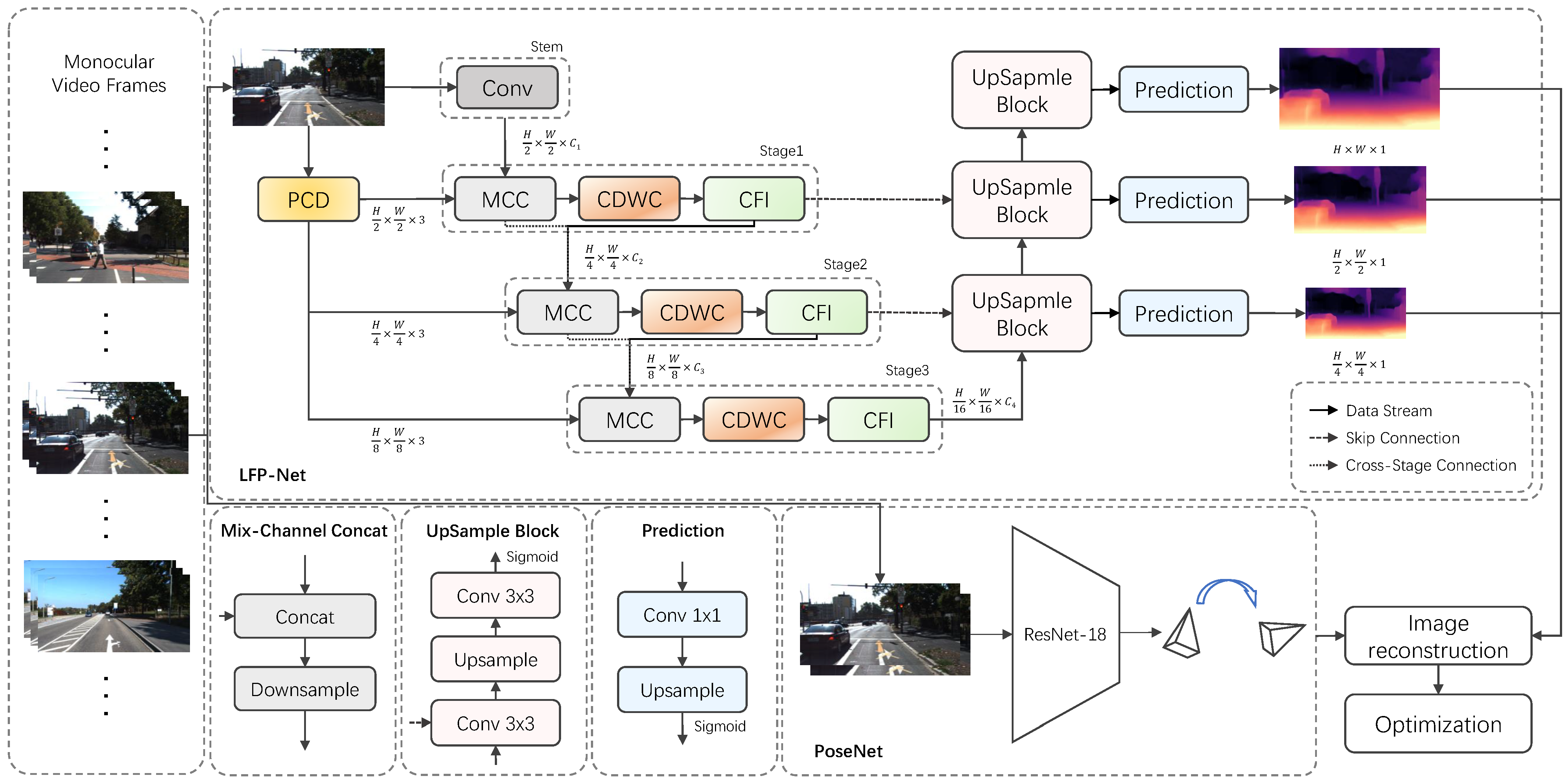
Figure 2.
Structure of Pooling Convolution Downsampling (PCD) module. N is the number of repetitions.
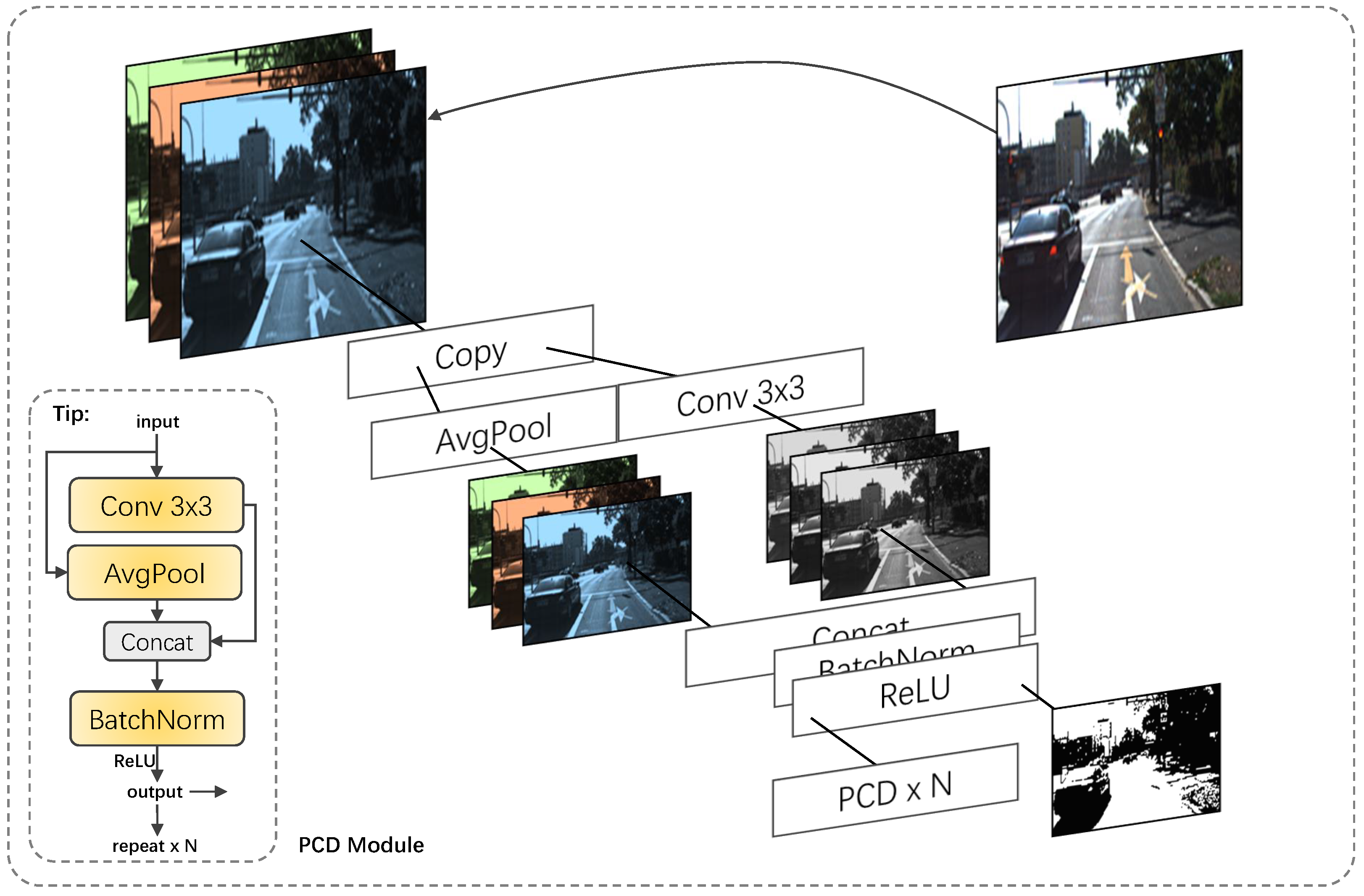
Figure 3.
On the left side of the figure, the design and structure of the proposed CDWC module are shown whereas the right side of the figure presents the receptive fields in the continuous dilated weighted convolution layers of the CDWC module using three different dilation rates; this will produce differing sizes of receptive fields.
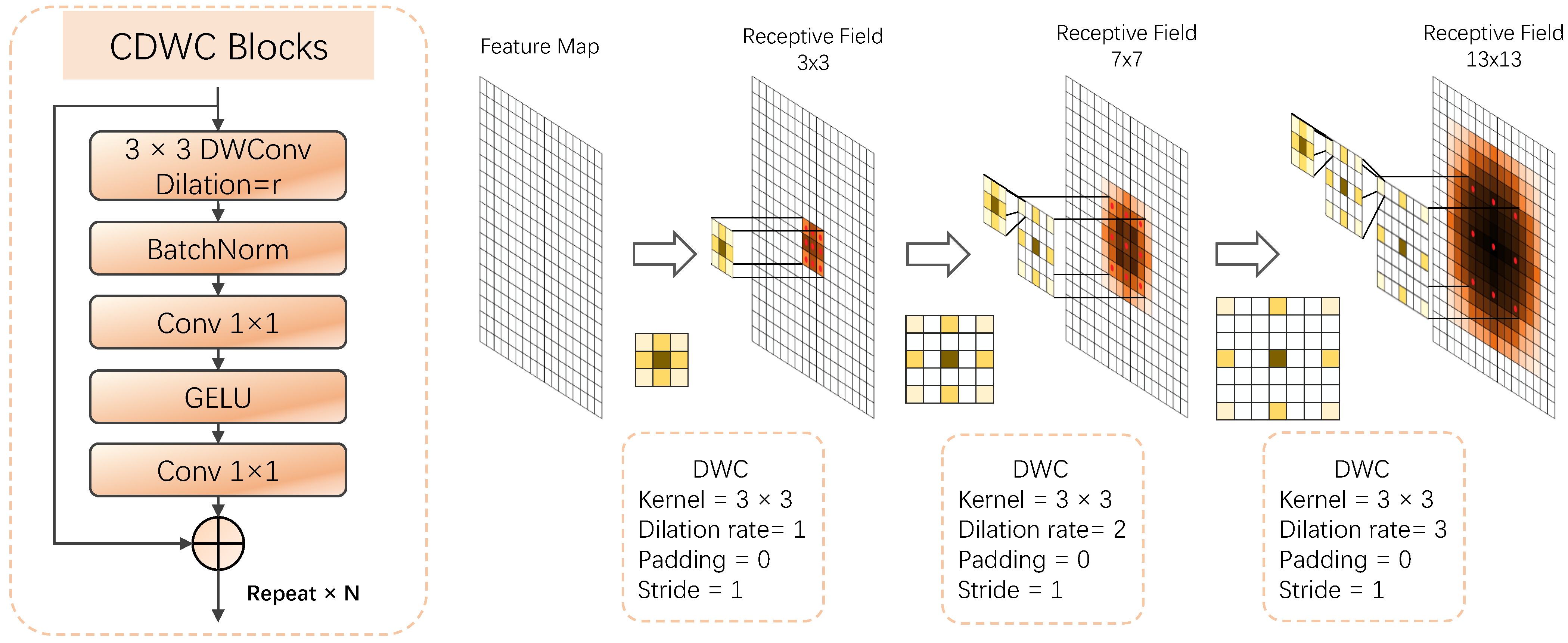
Figure 4.
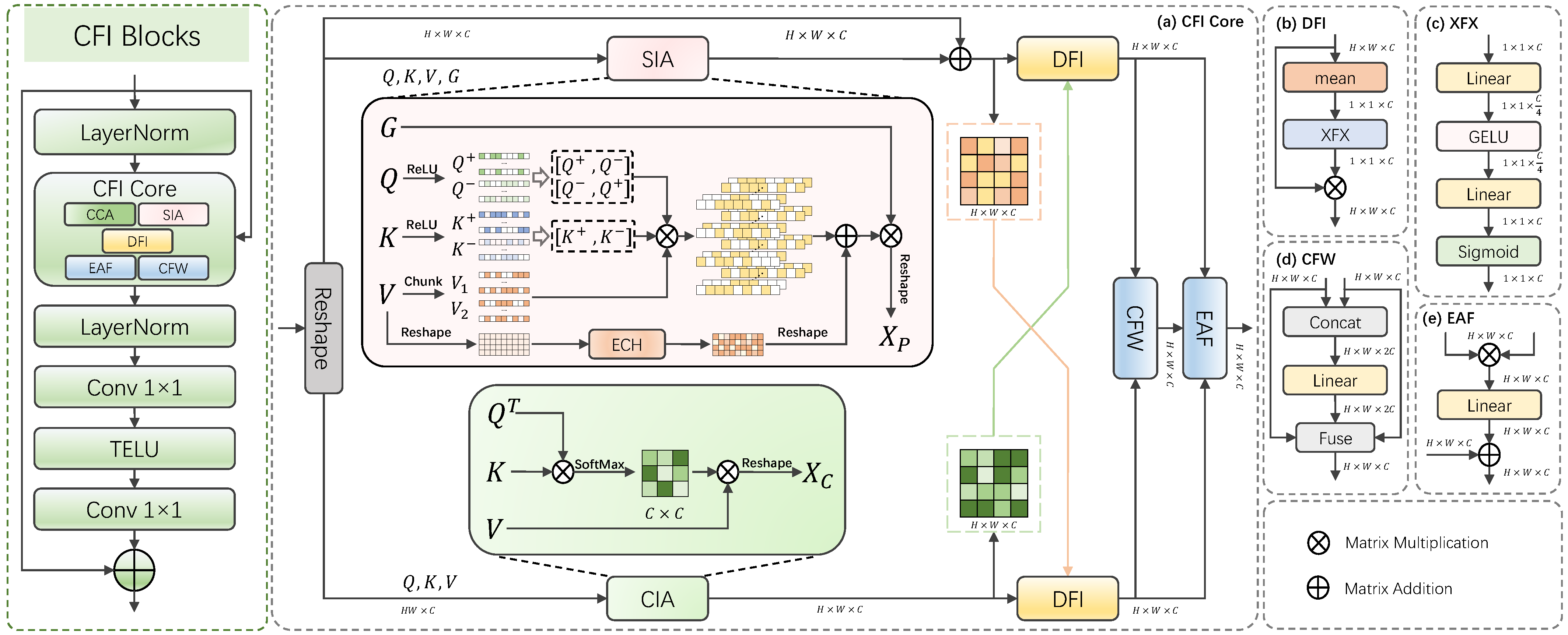
The left side provides a schematic overview of the proposed CFI module’s architecture. The right side shows the detailed structure of the primary sub-module within the CFI module.
LFP Encoder. The LFP encoder in LFP-Mono performs feature fusion using multi-scale features extracted across three stages, each equipped with corresponding downsampling, feature extraction, and attention modules. An RGB image of size H × W × 3 is input into the encoder, where the model duplicates the input and feeds it into both the feature extraction block and the pooling convolution block. The pooling convolution block provides pooled feature maps for the subsequent three stages. After passing through the feature extraction block, a feature map of size × × is obtained. In Stage 1, to minimize spatial information loss after multi-scale feature extraction, the model concatenates the input feature map with the pooled feature image, Afterwards, the feature map will be downsampled to a × × feature map, inspired by references [10,38]. Finally, through our designed CDWC and CFI modules, we can simultaneously capture global context and local features at multiple scales. The downsampling layers in Stage 1 and 2 both use the output of the proceeding downsampling layer as input features. This structure enables the model to effectively learn multi-scale and multi-stage features while preserving low-level detail features, serving a role similar to residual networks (ResNet) [3,37]. Similarly, after Stage 2 and Stage 3, feature maps of sizes × × and × × are output, respectively. The specific parameter settings for the LFP-Encoder can be found in Table 1.
Table 1.
Architecture of the Encoder in LFP-Net. [3 × 3, C] × 3 indicates that the Dilated Weighted Convolution (DWC) layers in the CDWC module employ 3 × 3 kernels and are stacked three times, with an output channel number of C. The “dilation” row specifies the dilation rates used in these three successive DWC convolutions. The PCD module uses ReLU as the activation function and the CDWC module uses GELU as the activation function.
LFP Decoder. Unlike using complex upsampling methods [11,39,40] or introducing additional attention modules, LFP-Mono uses a decoder similar to Lite-Mono’s depth decoder [10]. As shown in Figure 1, this structure expands the spatial dimension through bilinear upscaling and employs convolutional layers to perform residual connections on feature maps learned across the encoder’s three stages, along with feature learning concatenation from the preceding stage. The upsampled feature maps are then fed into the next higher-resolution upscaling module. Each upscaling module is followed by a feature reconstruction prediction head, ultimately outputting depth maps at different resolutions. These are used for image feature reconstruction, enabling the model to learn in a self-supervised manner.
3.3. Pooling Convolution Downsampling Module
The loss of spatial information due to downsampling operations has been a major issue affecting deep neural networks and their performance. For example, building textures and small object detail at low altitude are critical to the performance of many models, yet the traditional methods of downsampling (i.e., using pooling and strided convolution) often eliminate important detail information and thus reduce the ability to accurately capture local feature detail [41]. In this paper, we introduce a new type of downsampling module called the Pooling Convolution Downsampling (PCD) module, which will operate by combining both pooling and convolution processes in a formal, parallel manner. As shown in Figure 2, PCD allows for the adaptive extraction of critical features through parameter learning, providing a mechanism for preserving the structural information as well as the retention of global context information through pooling processes to reduce the interference of noise in the feature map. Our dual-branch fusion module differs from [42,43]. Our dual branch adopts a simple branch structure without unnecessary cross-inputs or multi-level branches. The PCD module will allow for the improved representation of features by combining local detail with global context to enhance the representation of features and to preserve spatial detail as much as possible while the resolution of the feature map is decreased.
Specifically, given an input feature map , it is processed through two parallel branches: the first branch performs feature extraction and downsampling through convolution, obtaining convolutional features , where is a 3 × 3 convolution. Then, the second branch uses a 2 × 2 average pooling operation (stride 2) for downsampling, obtaining pooled features :
The average pooling matches the feature map size at each stage. The features from both branches are then combined by concatenating them along the channel dimension, resulting in a fused feature set. Finally, channel adjustment and feature fusion are performed through a 3 × 3 convolutional layer. The output of the PCD module can be expressed as:
indicates a batch normalization layer followed by a ReLU activation function. n is the number of repetitions, which refers to the number of times the downsampling convolution is repeated, .
3.4. Continuous Dilated Weighted Convolution Module
Using lightweight convolutional neural networks, receptive field sizes are limited, making it extremely difficult for the model to detect smaller-sized objects. While dilated convolutions are often used to increase the receptive field size of the traditional methods [44], they do not always consider the edge characteristics of an object’s boundary and therefore lead to blurry edges when attempting to identify objects.This paper proposes the CDWC layer, which is based on the work of Cammarasana et al. [45]. The CDWC layer is built upon two concepts: sequential dilated convolutions and a feature-selection process. By stacking sequential dilated convolutional layers and progressively increasing the dilation-rate through those layers, the CDWC layer exponentially increases the size of the receptive field while maintaining high-resolution information and integrating long-distance contextual information. The CDWC layer also includes an embedded weighting mechanism that will enhance the response of features at the locations where the response is happening due to the discontinuity of the features, such as the edges or outlines of the object, and suppress the effect of extraneous background interference. As shown in Figure 3, after passing through three DWC modules with different dilation rates, the model will extract local features at multiple scales. Simultaneously, the weighted convolution assigns corresponding weights to edge features, allowing the model to learn more focused features without losing edge information, enhancing sensitivity to depth discontinuity regions. The dilation rate r controls the expansion of the effective receptive field. A dilated convolution achieves this by spacing the kernel elements with zeros, resulting in an effective kernel size of . Then, using a weight value to construct a centrosymmetric vector as , the weight matrix becomes . It is just like adjusting a telescope: selecting a suitable set of dilated rate and weighted parameters can maximize the model’s ’field of view’ and provide a more complete depth map, helping it select features for learning during training while avoiding the grid effect [46], to achieve more precise and clearer depth estimation.
Specifically, we have a feature map of size H × W × C to input into the model. When processing, it is first passed through a weighted dilated convolutional layer, which is mainly responsible for extracting local details from the feature map and increasing the number of channels. The actual process is as follows:
where is a 3 × 3 depthwise weighted dilated convolution with dilation rate r and weight array [0.5], and represents the BatchNorm layer. Then, the feature representation is refined through an inverted bottleneck structure, highlighting important information. is an n × 1 convolution, is a 1 × n convolution. This operation first converts the input to a spatial format for dimension transformation and activation, and then converts back to channel-first format after the activation function. This design ensures that the module simultaneously possesses local detail capture and global context information interaction capabilities. Finally, multi-scale feature information is added to yield the output:
The CDWC module consists of three DWC modules with different dilation rates connected in series:
3.5. Cross-Feature Interaction Module
Object structure plays a significant role in estimating depth within low-altitude images. The dilemma is that although one can analyze local details at various scales, there still tends to be no benefit in terms of understanding the overall correlations between objects, so when multiple objects share the same edges or colors as their background, many times, the resulting predictions by models are erroneous. Therefore, it appears that only using one-dimensional feature information may not sufficiently encode the spatial relationships of various objects. We have designed a model for this reason, which we call the Cross-Dimensional Feature Interaction (CFI) module. The CFI module merges the two different types of features that the CFI module learns through different dimensions (spatial and channels) so that it will allow the CFI module to comprehend the overall structure of a moving image while preserving the necessary amount of low-level spatial detail. As illustrated in Figure 4, the CFI module is comprised of two component modules; a Spatial Interaction Attention (SIA) module and a Channel Interaction Attention (CIA) module, as shown in Figure 4. The CFI module utilizes these two distinctive component modules to extract features from two distinctly different dimensions by performing feature extraction and learning in both spatial and channel dimensions. When the dimensionally extracted feature information is learned, it goes through a non-linear transformation so that the information can be successfully integrated with the image features. Next, the representations of the features are enhanced by employing a four-node inverted bottleneck structure in conjunction with the TeLU activation function that was proposed by Fernandez et al. [47], thereby promoting highly relevant feature information. We will present additional details regarding this process below.
Multi-dimensional Information Aggregation. The core structure of the CFI module consists of five parts: two attention parts, the Spatial Interaction Attention (SIA) part and the Channel Interaction Attention (CIA) part, and three feature processing parts, the Door-to-Door Information Fusion Interaction (DFI) part, the Channel Feature Interaction (CFW) part, and the Element-wise Adaptive Fusion (EAF) part, as shown in Figure 4a. The EAF and CFW components are adaptations of the work by Liu et al. [48] and Wang et al. [49]. The earliest use of this dual attention can be traced back to the work of Woo et al. [50] and Fu et al. [51]. The general concept is actually very similar, but the attention mechanism we use is different, as demonstrated in Figure 4d,e. The SIA and CIA parts take into account both the spatial feature space and its dimensional counterpart. The CFI module’s goal is to bridge local features and global relationships through concurrent computation of attention weights on both the spatial and channel dimensions. The spatial attention component enhances feature representations at critical spatial locations by emulating the contrast perception mechanism of the visual system, while the channel attention mechanism establishes global interdependencies among channels through cross-covariance computations. The module culminates in an adaptive gated fusion unit that enables profound interaction and complementarity between the two feature pathways.
Channel Interaction Attention. The CIA module models global contextual relationships through a channel-wise attention mechanism, inspired by Ali et al. [32]. Input features X, queries (Q), keys (K), and values (V) are generated through linear projection, and the computational complexity is reduced through a cross-covariance attention mechanism. Specifically, as illustrated in Figure 4a, the input feature is X; first, X is reshaped into (where N = H × W), then positional encoding is applied, and then queries, keys, and values of the same dimension are generated. The attention output of the CIA module is as follows:
where Q, K, and V are obtained by directly reshaping and splitting the input, , refers to the number of attention heads, and d refers to the dimension of each attention head. Softmax is applied along the channel dimension, reducing computational complexity from O(N2) to O(N). The output is weighted by a learnable scaling parameter and connected with the input via residuals:
Spatial Interaction Attention. The SIA module focuses on learning intra-channel features. Through polarity separation and feature interaction, it effectively enhances the model’s ability to capture detail features such as edge textures, establishes long-range dependencies in the spatial direction, and helps the model accurately lock onto target features, which is inspired by [52]. As illustrated in Figure 4a, the feature picture is input to the SIA module. We first linearly project (make into , where N = H × W) and separate the feature map for easy feature extraction and residual connection:
The separated input is transformed into the query (Q) via linear projection, while the key (K) and value (V) are generated from the input X through linear projections. Then, Q and K are passed through a ReLU activation function, respectively. The ReLU function sets all negative values to zero, thus naturally decomposing the features into two parts, [Q+, Q−] and [K+, K−], constructing positive and negative polarity features, further simulating the sensitivity mechanism of visual neurons to brightness, darkness, and contrast:
where , , , , the above reshape operations all changing the dimensions to . After extracting the polarity features, similarity and opposition query vectors are constructed through feature concatenation operations:
The construction of concatenates positive and negative polarity features along the channel dimension to form a “similarity” query vector. Its significance is to capture feature combinations that simultaneously have strong positive and strong negative responses, corresponding to high-contrast regions in vision. The construction of creates an “opposition” query vector by reversing the concatenation order. This simulates the ON/OFF opposition mechanism in the visual system, specifically handling mutually inhibitory relationships between features. The construction of integrates positive and negative key information, providing a key-value basis for subsequent attention calculation.
where is the mean of the key vectors along the sequence dimension (dim = −2), with dimension . is a numerical stability term, · denotes matrix multiplication, T denotes transpose operation. is the first part of the value vector, is the second part of the value vector, partitioned through a trunk operation. Then, and are concatenated along the channel dimension:
The value V is separately enhanced to enhance spatial feature representation, capturing local details and long-range dependencies:
where is a depthwise separable convolution, which can reduce computational load. Then, the attention output and enhanced value are fused through residual connection and gating to achieve adaptive control of the output:
3.6. Adaptive Dual Fusion Module
We found that simply adding features from the spatial and channel dimensions together does not fully utilize the feature information in each dimension. Therefore, we propose the Adaptive Dual Fusion module to fully utilize their information for interaction. As shown in Figure 4b, the DFI module part utilizes the global statistical information of the dual branches for cross-gating, enhancing feature complementarity, which is where the design inspiration of this module comes from. Let and represent the features, which can be expressed as follows:
where represents global average pooling: , is the Sigmoid function, which restricts the gating weights to the range [0, 1], ⊙ denotes element-wise multiplication, , etc. are learnable parameters of the MLP. Then, the outputs are input to the PTS module for weighted fusion:
Next, bilinear interaction captures the product interaction information between the dual-branch features, optionally enhancing nonlinear expressive capability:
where is a learnable scaling parameter, initially set to zero to ensure training stability. Finally, through layer scaling and dropout, training is stabilized and generalization is improved. Typically, the CFI module operates on an input feature map to produce an output that can be formulated as:
3.7. PoseNet Introduction
The reason why we use PoseNet for camera pose estimation is inspired by the work of [10,53]. Our entire method is also based on a self-supervised monocular depth estimation framework. Its core function is to predict the 6-DoF relative pose parameters (including 3D translation and 3D rotation) by inputting a pair of adjacent frames, the target image and the source image , to provide geometric constraints for view synthesis. PoseNet is jointly trained with the depth estimation network through minimization of the photometric reprojection loss, without requiring external pose annotations, significantly enhancing the model’s robustness and generalization ability in complex scenes.
3.8. Self-Supervised Learning
LFP-Mono employs a self-supervised learning framework trained on monocular video sequences, where depth estimation is formulated as a view synthesis task using photometric consistency between adjacent frames as the supervisory signal. Within this framework, the depth network generates the depth map for a target image , while the PoseNet estimates the relative camera pose transformation T between the target frame and a source frame (such as or ) [13]. Using the camera intrinsic matrix K, the source frame is then projected onto the target viewpoint to synthesize a reconstructed image , with the overall objective being to minimize the photometric reconstruction error between and while maintaining depth map smoothness.
The core of image reconstruction loss lies in the photometric reprojection process, which transforms the source image to the target viewpoint through geometric transformations. First, the predicted depth map and camera intrinsic parameters are used to backproject the target image pixels into 3D space. Subsequently, the estimated relative camera pose is applied to reproject them onto the source image plane. The photometric difference between the synthesized target view and the original target view serves as the primary supervision signal. The reconstruction loss process is as follows:
where G represents the image reconstruction function, is the source image, T is the camera pose transformation matrix, is the predicted depth map, and K is the camera intrinsic matrix. This formula clarifies that the generation of the reconstructed image relies on the joint optimization of depth prediction and pose estimation.
The image reconstruction loss measures the similarity between the synthetic image and the real image, combining the Structural Similarity Index (SSIM) [54] and the L1 norm to enhance robustness. The loss function is defined as:
where is a balancing weight (usually set to 0.85 [13]), SSIM captures structural information, and the L1 norm emphasizes pixel-level differences. To handle occlusion and moving objects, a multi-frame minimum photometric strategy is adopted [13]:
Here, s iterates over all source frames (such as forward and backward frames), and the frame with the smallest error is selected as the supervision signal. Additionally, invalid pixels (such as moving objects) are filtered using a binary mask M:
Finally, the image reconstruction loss is expressed as:
3.9. Edge-Aware Smoothness Loss
The depth map smoothness loss is used to avoid gradient discontinuities, typically based on gradient constraints of the depth map. This loss weakens smoothness at image edges to preserve object boundaries. The specific formula is [13,55]:
where is the normalized inverse depth ( is the predicted depth, is the mean), and represent horizontal and vertical gradients. The exponential term causes the smoothing weight to be inversely proportional to the image gradient, thus reducing the smoothing constraint in edge regions.
3.10. Total Loss Function and Multi-Scale Training
The total loss combines the reconstruction loss and smoothing loss of the image and is computed at different output scales to enhance feature consistency. Therefore, the total loss is defined as:
where is the smoothness term weight (usually set to ), and k indicates different scales. This multi-scale optimization helps the network capture hierarchical features and improves detail recovery.
4. Experiments
4.1. Datasets
KITTI. KITTI is one of the most widely utilized datasets for evaluating monocular depth estimation [14] methods. KITTI was initially collected to be used for research on autonomous vehicles and robots, and contains many examples of a variety of scene types, including urban, rural, highway, etc. KITTI also is a multi-modal dataset and contains many types of sensors that can be used for annotating data for depth estimation, stereo matching, and calculating visual odometry [56,57], including stereo cameras, LiDAR, and IMUs. The Eigen split is the most commonly used split for monocular depth estimation and includes approximately 39,180–39,810 training images, 4424 validation images, and 697 test images [24]. Because of its diversity in scene types and data completeness, KITTI has become one of the most important testbeds for evaluating monocular depth estimation algorithms (see Figure 5).
Figure 5.
Comparison of relative error, accuracy, and model size.
Make3D. The dataset contains RGB photographic images and their associated depth mapping images; furthermore, the dataset contains both photographic and depth mapping images of the same scene captured in outdoor environments (534 training and 134 testing). Each photographic image has a pixel resolution of 2272 × 1704, enabling these images to maintain good detail and realistic representation. Make3D has been commonly used as a benchmark dataset for measuring how well a model generalises over multiple distributions of data (i.e., differences in scene data types) or previously unseen scenes.
Syndrone. The Syndrone dataset is a low-altitude perspective simulation dataset primarily featuring urban low-altitude scenes, with a portion of suburban low-altitude scenes, having 72,000 images. In addition to following the trends of previously developed datasets, Syndrone provides much greater diversity of perspective—also including depth maps. The types of tasks that Syndrone supports are many, including semantic segmentation, object localization, object tracking, and 3D reconstruction. Following the trend of the previously created datasets, the authors manually segmented the data and placed each sub-sample into the training and test sets. There are 60,000 samples within the training set and 12,000 samples throughout the testing set—both sets were collected through a combination of eight uniquely designed “virtual” cities located in eight separate virtual city environments. Acquisition of the data was conducted using an improved version of the CARLA Simulator, at flight altitudes of 20 m, 50 m, and 80 m; this corresponds to view angles of 30 degrees, 60 degrees, and 90 degrees, respectively. With an acquisition frame rate of 25 Hz, Syndrone offers a diverse temporal and spatial perspective of the low-altitude environment.
4.2. Training Settings and Implementation Details
Experimental Details and Hyperparameters. We implemented the LFP-Mono model using PyTorch [58], training for 50 epochs with a batch size of 12 and an input resolution of 640 × 192 on a single NVIDIA 3080ti GPU. AdamW [59] was employed as the model optimizer for learning weight parameters, with a weight decay coefficient of 1 × 10⁻². DropPath [60] was incorporated into both the CDWC and CFI modules to enhance robustness and mitigate model overfitting. The initial learning rate for LFP-net was set to 5 × 10⁻⁴, utilizing a cosine learning rate decay strategy. Most of the above hyperparameters refer to the settings in [10], and their values have been searched and optimized in previous work.
Data Augmentation. Augmenting the dataset helps create a more robust model and improves the generalization ability of the model to learn and adapt on a much larger scale due to the varying amounts of data available. Examples of how augmentation can increase the robustness and generalization ability include images that are flipped horizontally, with a probability of 50%. Randomly changing brightness, saturation, contrast (+/−0.2), and hue (+/−0.1), and many other augmentation options will be used.
Evaluation Metrics. The proposed model was evaluated against several baselines using established metrics [24]. The Absolute Relative Error (Abs Rel) serves to assess global accuracy by computing the mean absolute relative difference between predictions and ground truth. In contrast, the Squared Relative Error (Sq Rel) penalizes larger errors more severely by squaring the differences. The Root Mean Square Error (RMSE) reflects overall prediction precision, while its logarithmic variant, RMSE log, operates in the log domain to better handle varying depth scales. Additionally, threshold accuracy measures the proportion of pixels where the predicted-to-ground-truth depth ratio falls within a specified tolerance, specifically for , , and . The corresponding formulas are as follows:
In this formula, N refers to the total number of pixels in the depth map. For each pixel i, we use to represent the predicted depth value, while represents its actual correct depth value.
4.3. KITTI Results
We compare our proposed LFP-Mono model with other well-known monocular depth estimation models on the KITTI dataset, with evaluation results shown in Table 2 and Figure 6. To ensure consistency, we set the input image resolution to 640 × 192, matching that of other models. Additionally, we did not incorporate any pre-training and consistency in subsequent experiments on other datasets. Our model outperforms other self-supervised models across all evaluation metrics while requiring the fewest parameters and computational cost. Within the accuracy metric , our model demonstrates a significant lead over competitors, indicating its capability to predict more precise and detailed depth maps. Specifically, LFP-Mono significantly outperforms Monodepth2 [13], which uses ResNet50 [46] as the backbone network, and our model parameters are only 6% of its parameters. Compared to the recently popular lightweight networks Lite-Mono [10] and FSLNet-L [26], our method achieves superior results with fewer parameters. As shown in Figure 6, in instance comparison experiments against Lite-Mono and Monodepth2, our model demonstrates greater accuracy in depth estimation for details such as object edges and small objects near road edges.
Table 2.
Depth estimation results on the KITTI dataset using the Eigen split [14]. All inputs are resized to 640 × 192 resolution. The best-performing results are highlighted in bold, and the second-best are underlined. M†: Models without pre-training on ImageNet [61]. M: Models with pre-training on ImageNet. ↓: The higher the value, the better the performance. ‘↑’: The lower the value, the better the performance. The same evaluation indicator will not be repeated later. The result is based on a single run.
Figure 6.
Qualitative results on the KITTI dataset. This figure presents depth maps generated by Monodepth2 [13], Lite-Mono [10], and our LFP-Mono. Evident from the regions highlighted in yellow boxes, compared to our model, other models lose object boundary information and fine details in their predicted depth maps, due to limitations in perceptual capability and receptive field.
4.4. Make3D Results
Our proposed model was evaluated on the Make3D [15] dataset to test its generalization ability in different outdoor scene environments. We used the model trained on the KITTI [14] dataset without any fine-tuning and directly performed inference prediction on the Make3D dataset. Table 3 shows that LFP-Mono outperforms the other three methods. Figure 7 and Table 3 show some qualitative results, indicating that the proposed model generates more precise details and object edges in untrained scenes, while being able to perceive objects of different sizes, demonstrating excellent generalization ability.
Table 3.
Depth estimation results on the Make3D dataset. All models were first trained on the KITTI dataset and then directly tested on Make3D without any fine-tuning. The best-performing results are highlighted in bold. The result is based on a single run.
Figure 7.
Qualitative results on the Make3D dataset. The yellow boxes show clearly visible variation. While all methods demonstrate a significant ability to perceive and create environmental structural and boundary information, our method has greater strength in both areas.
4.5. Syndrone Results
Following the completion of the training on KITTI, we applied the depth estimation model on different segments of actual low-altitude videos. The results showed that although our model had been able to generalize to some extent in low-altitude situations, its ability to perform under certain circumstances (i.e., reflections from building windows and low-flying objects) was weak, especially at the edge of tall buildings and when they were located near the camera. In order to improve performance, we performed a retraining of the model using synthetic low-altitude data from Syndrone set up with an input resolution of 640 × 192. The training approach taken was the same approach used with the KITTI data, so we did not use any pre-trained weights to train the model using the Syndrone dataset [16]. At the same time, the training hyperparameters are consistent with the KITTI experiments As can be seen in Figure 8 and Table 4 showing the results on testing after training on the Syndrone set, LFP-Mono performed better than many other self-supervised methods across all evaluation metrics and has fewer parameters than the other methods. Furthermore, using the same model trained on both KITTI and Syndrone, we observed that the Syndrone-trained model generates more precise and detailed depth maps in real low-altitude scenarios, as illustrated in Figure 9. These results demonstrate that the Syndrone dataset is highly valuable for depth estimation in drone applications. It not only achieves higher accuracy in detecting building edges but also demonstrates strong generalization capabilities in perceiving objects of varying sizes, even within complex environments.
Figure 8.
Qualitative results on the Syndrone dataset. Representative differences are highlighted in yellow boxes.
Table 4.
Results on the Syndrone dataset. No pre-trained weights were used. ↓: The higher the value, the better the performance. ‘↑’: The lower the value, the better the performance. The best-performing results are highlighted in bold, and the second-best are underlined. The results are based on a single run.
Figure 9.
Real-world test results of the same model architecture trained on KITTI and Syndrone, respectively. The areas within the yellow rectangles show significant differences.
4.6. Ablation Study on Model Architectures
To further validate the usefulness of each module in our network, we conducted the following ablation studies on KITTI: we progressively deleted modules from LFP-Mono (our new model) and quantitatively analysed how each design choice influences the depth estimation results. Results are shown in Table 5 and modules will be described as necessary.
Table 5.
Ablation study on the dilation rates. The best scores are marked in bold.
Benefits of Cross-stage Connections. When cross-scale connections are removed from the model all depth estimation error metrics increase, indicating that residual pathways between feature maps at different levels assist the fusion of cross-scale information. The reliance on these connections implies that the model may struggle to effectively integrate shallow information into the depths of the model during inference. Comparative metrics of parameters between the two networks demonstrate a negligible increase to the total parameter count and the computational cost.
Benefits of Pooling Connections. The PCD module is used to overcome loss of spatial information. We remove the PCD module in the mobile variant of our model. It led to AbsRel increasing from 0.114 to 0.120, with model parameters decreasing only slightly. This is an indication that the PCD module allows the model to be more capable of ‘retaining’ detail by pooling and aggregating global multi-level spatial information. It is clear that at the cost of a small increase for parameters, we are able to improve feature extraction capabilities in augmenting the model itself under limited overhead.
Benefits of CDWC. The CDWC component was implemented so that multi-scale contextual information could be acquired gradually as the image is downsampled. Setting aside the CDWC component, all depth error metrics increased considerably while reducing the number of model parameters significantly: we see that the Absolute Relative Error rose to 0.128 and that the model’s Accuracy for < 1.25 decreased to 0.845 as a result of using parallel convolutional layers with multiple dilation rates. Therefore, these findings demonstrate how the use of parallel convolutions with varying dilation rates allows for extraction of multi-scale features and improvement of local detail recovery in a more efficient manner than adding additional training parameters.
Benefits of CFI. The establishment of long-range spatial dependencies is a major function of the CFI module. While removing the CFI module from this architecture would create a much simpler model architecture consisting of only 1.426M parameters, the performance of this simpler model will be significantly decreased. Thus, the CFI module plays an integral role in providing the global context necessary to build the long-range spatial dependencies that would be lacking in the model due to the convolutional operations’ restricted spatial locality limitations.
4.7. Ablation Study on Dilation Rates
Initially, to investigate the optimal performance of the proposed CDWC module under different dilation rates—that is, to identify the optimal dilation rate—we designed multiple sets of comparative experiments. To reiterate, our proposed CDWC module consists of three consecutive dilated weighted convolutions (DWC), each employing a distinct dilation rate. In the experiments, we referenced the dilation rates setting rules proposed by Luo et al. [62] in their paper. The specific experimental settings are as follows: (1) The dilation rates for each group were set to 1, 1, 1, as a baseline for evaluating the effectiveness of weighted dilated convolutions; (2) The dilation rates for each group were set to 1, 2, 3 to validate the multi-scale feature extraction capability; (3) Considering that larger dilation rates can extract higher-level features, we set a group with larger dilation parameters: the first two groups with dilation rates of 1, 2, 3 and the last group with 1, 2, 5 to enhance the receptive field of deep features; (4) As a comparison, we set a group where all dilation rates are 1, 2, 5 to further examine the impact of larger dilation rates.
The experimental results are shown in Table 6. Comparing (1) and (2) reveals that introducing a moderate dilation rate helps improve performance. Meanwhile, experimental group (3) achieved the best results across multiple metrics, indicating that appropriately increasing the dilation rate in deeper layers enhances the model’s ability to express semantic features. However, blindly using a larger dilation rate leads to a decline in model performance, as evidenced by experimental group (4). It is evident that excessively high void ratios are detrimental to the perception of small and medium-sized objects. Therefore, configuration (3) is ultimately adopted in this method to achieve balanced extraction of multi-scale local features between shallow and deep layers.
Table 6.
Ablation study on the model architecture. All inputs use a resolution of 640 × 192. Training was conducted from scratch without using any pre-trained weights or fine-tuning. ↓: The higher the value, the better the performance. ‘↑’: The lower the value, the better the performance. The best score is marked in bold. w/o: Means without, this module has been completely removed.
4.8. Complexity and Inference Speed Analysis
To evaluate the efficiency of our model’s depth estimation, we compare LFP-Mono with Monodepth2 [13], R-MSFM6 [40], and Lite-Mono [10] in terms of parameter count and inference speed on an RTX 3080 Ti GPU. As shown in Table 7, our proposed LFP-Mono achieves a favorable balance between parameter count and speed. Its encoder is lighter than other methods while maintaining low computational overhead. Although slightly slower in inference speed, it demonstrates higher efficiency compared to the large-parameter design of Monodepth2. R-MSFM6 suffers from slower evaluation speeds on real images due to the recurrent multiscale structure in its decoder, Lite Mono’s encoder uses deeper convolutions, the network becomes wider, resulting in a larger overall model size. Overall, LFP-Mono represents an efficient and compact architecture suitable for resource-constrained edge deployments.
Table 7.
Model complexity and inference speed evaluation. We compare the number of Params, FLOPs, and speed. All inputs use a resolution of 640 × 192. The best scores are marked in bold.
5. Discussion
Our LFP-Mono model stands strong against traditional benchmarks like KITTI, and demonstrates impressive generalization on Make3D and Syndrone. Some limitations and possible directions for future work are given below. For the LFP-Net framework, the implementation of the CDWC and CFI modules strikes a good balance between efficiency and representation of features; however, its treatment of highly dynamic objects or drastic occlusions is still a challenge, as with most self-supervised depth estimation works. The weight matrices used in the CDWC module could be trained even further. Finally, lightweight models would consistently fail to recover fine depth details in the scence of textured regions or near object boundaries, although this is slightly to be expected when working with larger and more supervised models. Although the dual-path network in our CFI module is able to easily fuse the features together, it also may slow the runtime down on limited hardware, even with the small performance gain. At the same time, in this study, we did not specifically evaluate the performance in dynamic scenarios, which will be one of our future research tasks. With datasets, we plainly noticed limited generalizability when training on Kitti on a barebones model, and used real-world tests at low-altitude perspectives. What is interesting to note is that training models on the synthetic Syndrone dataset still yielded generalization also on real-world images. In Figure 9, we expose the LFP-Monomodel to both the KITTI ground-level dataset and the Syndrone datasets and train both models upon them, and then expose it to low-altitude flight video sequences garnered from the real world. Though Syndrone is synthetic, models trained on it outperformed the ground-level models trained on Kitti in the real world, experimentally tackling buildings with strong specular reflection and irregular geometries. We were surprised that the model even recognized flying objects that were not visualized during training. These findings not only develop LFP-Mono’s reach to more degraded real-world images which it would probably be used for, but some are also applicable to the growth of knowledge in solving niche problems, such as narrow data-scattered low-altitude scenarios, and employing depth estimation itself for visual-obstacle-avoidance for drones. For visual obstacle avoidance for drones, we will consider integrating the work of target tracking and target recognition in the future to roughly form a visual obstacle avoidance decision system for UAVs. Through multimodal data and multi-method fusion, we may be able to achieve reliable visual obstacle avoidance effects at a very low cost.
6. Conclusions
This paper introduces LFP-Mono, a lightweight self-supervised monocular depth estimation model. With hybrid CNN-Transformer architecture, the model balances multi-scale features and long-range global contextual information while capturing object detail recognition in scenes. We designed PCD, helping to reduce information loss during downsampling without compromising detail and local features. The CDWC module increases local feature learning ability and learning of multi-scale information, while the CFI module allows local-global feature interaction so that LFP-Mono can perceive far and near targets. Experiments on the KITTI dataset verify our method’s strength. Tests on Make3D show strong generalization capability, while experimental results on the Syndrone low-altitude synthetic dataset show the model adapting well to complex scenarios. We can enjoy balance between model complexity and inference speed.
Author Contributions
Conceptualization, H.C. and J.L.; methodology, H.C. and J.L.; software, J.L.; validation, J.L.; formal analysis, J.L. and Y.Z.; data curation, J.L.; writing—original draft preparation, J.L.; writing—review and editing, H.C., J.L., and J.Z.; visualization, J.L.; supervision, J.X., Y.Z., and Q.Y.; project administration, H.C. and J.Z.; funding acquisition, H.C. All authors have read and agreed to the published version of the manuscript.
Funding
This research was funded by Guangdong Province Special Fund for Science and Technology (“major special projects + task list”) Project (No. STKJ202209017), Guangdong Science and Technology Plan Projects (No. STKJ2023012).
Data Availability Statement
The KITTI dataset is available online at https://www.cvlibs.net/datasets/kitti/eval_depth.php?benchmark=depth_completion (accessed on 28 November 2025); The Make3D dataset is available online at http://make3d.cs.cornell.edu/data.html (accessed on 28 November 2025); The Syndrone dataset is available online at https://github.com/LTTM/Syndrone (accessed on 28 November 2025).
Acknowledgments
We would like to express our gratitude to all those who have helped with this work and to the authors. We also wish to thank the ‘Key Laboratory of Frontier Mathematics and Large Model Computing, Guangdong Provincial Universities’ for its generous support.
Conflicts of Interest
The authors declare no conflicts of interest.
References
- Carion, N.; Massa, F.; Synnaeve, G.; Usunier, N.; Kirillov, A.; Zagoruyko, S. End-to-end object detection with transformers. In Proceedings of the European Conference on Computer Vision, Virtual, 23–28 August 2020; pp. 213–229. [Google Scholar]
- Ramamonjisoa, M.; Du, Y.; Lepetit, V. Predicting sharp and accurate occlusion boundaries in monocular depth estimation using displacement fields. In Proceedings of the IEEE/CVF Conference on Computer Vision and Pattern Recognition, Virtual, 14–19 June 2020; pp. 14648–14657. [Google Scholar]
- Laina, I.; Rupprecht, C.; Belagiannis, V.; Tombari, F.; Navab, N. Deeper depth prediction with fully convolutional residual networks. In Proceedings of the 2016 Fourth International Conference on 3D Vision, Stanford, CA, USA, 25–28 October 2016; pp. 239–248. [Google Scholar]
- Fu, H.; Gong, M.; Wang, C.; Batmanghelich, K.; Tao, D. Deep ordinal regression network for monocular depth estimation. In Proceedings of the IEEE Conference on Computer Vision and Pattern Recognition, Salt Lake City, UT, USA, 18–22 June 2018; pp. 2002–2011. [Google Scholar]
- Zhou, T.; Brown, M.; Snavely, N.; Lowe, D.G. Unsupervised learning of depth and ego-motion from video. In Proceedings of the IEEE Conference on Computer Vision and Pattern Recognition, Honolulu, HI, USA, 21–26 July 2017; pp. 1851–1858. [Google Scholar]
- Godard, C.; Mac Aodha, O.; Brostow, G.J. Unsupervised monocular depth estimation with left-right consistency. In Proceedings of the IEEE Conference on Computer Vision and Pattern Recognition, Honolulu, HI, USA, 21–26 July 2017; pp. 270–279. [Google Scholar]
- Zhao, C.; Sun, Q.; Zhang, C.; Tang, Y.; Qian, F. Monocular depth estimation based on deep learning: An overview. Sci. China Technol. Sci. 2020, 63, 1612–1627. [Google Scholar] [CrossRef] [Scilit]
- Yin, Z.; Shi, J. Geonet: Unsupervised learning of dense depth, optical flow and camera pose. In Proceedings of the IEEE Conference on Computer Vision and Pattern Recognition, Salt Lake City, UT, USA, 18–22 June 2018; pp. 1983–1992. [Google Scholar]
- Kumar, V.R.; Klingner, M.; Yogamani, S.; Milz, S.; Fingscheidt, T.; Mader, P. Syndistnet: Self-supervised monocular fisheye camera distance estimation synergized with semantic segmentation for autonomous driving. In Proceedings of the IEEE/CVF Winter Conference on Applications of Computer Vision, Virtual, 5–9 January 2021; pp. 61–71. [Google Scholar]
- Zhang, N.; Nex, F.; Vosselman, G.; Kerle, N. Lite-mono: A lightweight cnn and transformer architecture for self-supervised monocular depth estimation. In Proceedings of the IEEE/CVF Conference on Computer Vision and Pattern Recognition, Vancouver, BC, Canada, 17–24 June 2023; pp. 18537–18546. [Google Scholar]
- Zhao, C.; Zhang, Y.; Poggi, M.; Tosi, F.; Guo, X.; Zhu, Z.; Huang, G.; Mattoccia, S. Monovit: Self-supervised monocular depth estimation with a vision transformer. In Proceedings of the 2022 International Conference on 3D Vision, 3DV, Virtual, 12–15 September 2022; pp. 668–678. [Google Scholar]
- Ranftl, R.; Bochkovskiy, A.; Koltun, V. Vision transformers for dense prediction. In Proceedings of the IEEE/CVF International Conference on Computer Vision, Virtual, 11–17 October 2021; pp. 12179–12188. [Google Scholar]
- Godard, C.; Mac Aodha, O.; Firman, M.; Brostow, G.J. Digging into self-supervised monocular depth estimation. In Proceedings of the IEEE/CVF International Conference on Computer Vision, Seoul, Republic of Korea, 27 October–2 November 2019; pp. 3828–3838. [Google Scholar]
- Geiger, A.; Lenz, P.; Stiller, C.; Urtasun, R. Vision meets robotics: The kitti dataset. Int. J. Robot. Res. 2013, 32, 1231–1237. [Google Scholar] [CrossRef] [Scilit]
- Saxena, A.; Sun, M.; Ng, A.Y. Make3d: Learning 3d scene structure from a single still image. IEEE Trans. Pattern Anal. Mach. Intell. 2008, 31, 824–840. [Google Scholar] [CrossRef] [Scilit] [PubMed]
- Rizzoli, G.; Barbato, F.; Caligiuri, M.; Zanuttigh, P. Syndrone-multi-modal uav dataset for urban scenarios. In Proceedings of the IEEE/CVF International Conference on Computer Vision, Paris, France, 2–6 October 2023; pp. 2210–2220. [Google Scholar]
- Garg, R.; Bg, V.K.; Carneiro, G.; Reid, I. Unsupervised cnn for single view depth estimation: Geometry to the rescue. In Proceedings of the European Conference on Computer Vision, Amsterdam, The Netherlands, 11–14 October 2016; pp. 740–756. [Google Scholar]
- Bian, J.; Li, Z.; Wang, N.; Zhan, H.; Shen, C.; Cheng, M.M.; Reid, I. Unsupervised scale-consistent depth and ego-motion learning from monocular video. In Advances in Neural Information Processing Systems; 2019; Volume 32. [Google Scholar]
- Casser, V.; Pirk, S.; Mahjourian, R.; Angelova, A. Unsupervised monocular depth and ego-motion learning with structure and semantics. In Proceedings of the IEEE/CVF Conference on Computer Vision and Pattern Recognition Workshops, Long Beach, CA, USA, 16–20 June 2019; pp. 381–388. [Google Scholar]
- Cho, J.; Min, D.; Kim, Y.; Sohn, K. Deep monocular depth estimation leveraging a large-scale outdoor stereo dataset. Expert Syst. Appl. 2021, 178, 114877. [Google Scholar] [CrossRef] [Scilit]
- Chen, W.; Fu, Z.; Yang, D.; Deng, J. Single-image depth perception in the wild. In Advances in Neural Information Processing Systems; The MIT Press: Cambridge, MA, USA, 2016; Volume 29. [Google Scholar]
- Gur, S.; Wolf, L. Single image depth estimation trained via depth from defocus cues. In Proceedings of the IEEE/CVF Conference on Computer Vision and Pattern Recognition, Long Beach, CA, USA, 16–20 June 2019; pp. 7683–7692. [Google Scholar]
- Masoumian, A.; Rashwan, H.A.; Abdulwahab, S.; Cristiano, J.; Asif, M.S.; Puig, D. GCNDepth: Self-supervised monocular depth estimation based on graph convolutional network. Neurocomputing 2023, 517, 81–92. [Google Scholar] [CrossRef] [Scilit]
- Eigen, D.; Puhrsch, C.; Fergus, R. Depth map prediction from a single image using a multi-scale deep network. In Proceedings of the Advances in Neural Information Processing Systems, Montreal, QC, Canada, 8–13 December 2014; Volume 27. [Google Scholar]
- Dosovitskiy, A.; Beyer, L.; Kolesnikov, A.; Weissenborn, D.; Zhai, X.; Unterthiner, T.; Dehghani, M.; Minderer, M.; Heigold, G.; Gelly, S.; et al. An Image is Worth 16 × 16 Words: Transformers for Image Recognition at Scale. In Proceedings of the International Conference on Learning Representations, Virtual, 3–7 May 2021. [Google Scholar]
- Jia, S.; Yao, W. Joint learning of frequency and spatial domains for dense image prediction. ISPRS J. Photogramm. Remote Sens. 2023, 195, 14–28. [Google Scholar] [CrossRef] [Scilit]
- Hoiem, D.; Efros, A.A.; Hebert, M. Automatic photo pop-up. In Proceedings of the ACM SIGGRAPH 2005, Los Angeles, CA, USA, 31 July–4 August 2005; pp. 577–584. [Google Scholar]
- Cai, H.; Li, J.; Hu, M.; Gan, C.; Han, S. Efficientvit: Lightweight multi-scale attention for high-resolution dense prediction. In Proceedings of the IEEE/CVF International Conference on Computer Vision, Paris, France, 2–6 October 2023; pp. 17302–17313. [Google Scholar]
- Varma, A.; Chawla, H.; Zonooz, B.; Arani, E. Transformers in self-supervised monocular depth estimation with unknown camera intrinsics. arXiv 2022, arXiv:2202.03131. [Google Scholar] [CrossRef] [Scilit]
- Yang, L.; Kang, B.; Huang, Z.; Xu, X.; Feng, J.; Zhao, H. Depth anything: Unleashing the power of large-scale unlabeled data. In Proceedings of the IEEE/CVF Conference on Computer Vision and Pattern Recognition, Seattle, WA, USA, 16–22 June 2024; pp. 10371–10381. [Google Scholar]
- Jia, S.; Pei, X.; Yao, W.; Wong, S.C. Self-supervised depth estimation leveraging global perception and geometric smoothness. IEEE Trans. Intell. Transp. Syst. 2022, 24, 1502–1517. [Google Scholar] [CrossRef] [Scilit]
- Ali, A.; Touvron, H.; Caron, M.; Bojanowski, P.; Douze, M.; Joulin, A.; Laptev, I.; Neverova, N.; Synnaeve, G.; Verbeek, J.; et al. Xcit: Cross-covariance image transformers. In Proceedings of the Advances in Neural Information Processing Systems, Virtual, 6–14 December 2021; Volume 34, pp. 20014–20027. [Google Scholar]
- Agarwal, A.; Arora, C. Depthformer: Multiscale vision transformer for monocular depth estimation with local global information fusion. arXiv 2022, arXiv:2207.04535. [Google Scholar] [CrossRef] [Scilit]
- Xu, C.; Huang, B.; Elson, D.S. Self-supervised monocular depth estimation with 3-d displacement module for laparoscopic images. IEEE Trans. Med. Robot. Bionics 2022, 4, 331–334. [Google Scholar] [CrossRef] [Scilit]
- Lyu, X.; Liu, L.; Wang, M.; Kong, X.; Liu, L.; Liu, Y.; Chen, X.; Yuan, Y. Hr-depth: High resolution self-supervised monocular depth estimation. In Proceedings of the AAAI Conference on Artificial Intelligence, Virtual, 2–9 February 2021; Volume 35, pp. 2294–2301. [Google Scholar]
- Wofk, D.; Ma, F.; Yang, T.J.; Karaman, S.; Sze, V. Fastdepth: Fast monocular depth estimation on embedded systems. In Proceedings of the 2019 International Conference on Robotics and Automation, Montreal, QC, Canada, 20–24 May 2019; pp. 6101–6108. [Google Scholar]
- Yan, J.; Zhao, H.; Bu, P.; Jin, Y. Channel-wise attention-based network for self-supervised monocular depth estimation. In Proceedings of the 2021 International Conference on 3D Vision, Virtual, 1–3 December 2021; pp. 464–473. [Google Scholar]
- Mehta, S.; Rastegari, M.; Shapiro, L.; Hajishirzi, H. Espnetv2: A light-weight, power efficient, and general purpose convolutional neural network. In Proceedings of the IEEE/CVF Conference on Computer Vision and Pattern Recognition, Long Beach, CA, USA, 16–20 June 2019; pp. 9190–9200. [Google Scholar]
- Bae, J.; Moon, S.; Im, S. Deep digging into the generalization of self-supervised monocular depth estimation. In Proceedings of the AAAI Conference on Artificial Intelligence, Washington, DC, USA, 7–14 February 2023; Volume 37, pp. 187–196. [Google Scholar]
- Zhou, Z.; Fan, X.; Shi, P.; Xin, Y. R-msfm: Recurrent multi-scale feature modulation for monocular depth estimating. In Proceedings of the IEEE/CVF International Conference on Computer Vision, Virtual, 11–17 October 2021; pp. 12777–12786. [Google Scholar]
- Dai, D.; Dong, C.; Yang, X.; Li, Z.; Xu, S. Striking a better balance between segmentation performance and computational costs with a minimalistic network design. Appl. Soft Comput. 2025, 182, 113549. [Google Scholar] [CrossRef] [Scilit]
- Chen, Y.; Li, J.; Xiao, H.; Jin, X.; Yan, S.; Feng, J. Dual path networks. In Advances in Neural Information Processing Systems; The MIT Press: Cambridge, MA, USA, 2017; Volume 30. [Google Scholar]
- Szegedy, C.; Vanhoucke, V.; Ioffe, S.; Shlens, J.; Wojna, Z. Rethinking the inception architecture for computer vision. In Proceedings of the IEEE Conference on Computer Vision and Pattern Recognition, Las Vegas, NV, USA, 27–30 June 2016; pp. 2818–2826. [Google Scholar]
- Yu, F.; Koltun, V. Multi-scale context aggregation by dilated convolutions. arXiv 2015, arXiv:1511.07122. [Google Scholar]
- Cammarasana, S.; Patanè, G. Optimal Weighted Convolution for Classification and Denosing. arXiv 2025, arXiv:2505.24558. [Google Scholar] [CrossRef] [Scilit]
- He, K.; Zhang, X.; Ren, S.; Sun, J. Deep residual learning for image recognition. In Proceedings of the IEEE Conference on Computer Vision and Pattern Recognition, Las Vegas, NV, USA, 27–30 June 2016; pp. 770–778. [Google Scholar]
- Fernandez, A. TeLU Activation Function for Fast and Stable Deep Learning. Master’s Thesis, University of South Florida, Tampa, FL, USA, 2024. [Google Scholar]
- Liu, S.; Huang, D.; Wang, Y. Learning spatial fusion for single-shot object detection. arXiv 2019, arXiv:1911.09516. [Google Scholar] [CrossRef] [Scilit]
- Wang, G.; Wang, K.; Lin, L. Adaptively connected neural networks. In Proceedings of the IEEE/CVF Conference on Computer Vision and Pattern Recognition, Long Beach, CA, USA, 16–20 June 2019; pp. 1781–1790. [Google Scholar]
- Woo, S.; Park, J.; Lee, J.Y.; Kweon, I.S. Cbam: Convolutional block attention module. In Proceedings of the European Conference on Computer Vision, Munich, Germany, 8–14 September 2018; pp. 3–19. [Google Scholar]
- Fu, J.; Liu, J.; Tian, H.; Li, Y.; Bao, Y.; Fang, Z.; Lu, H. Dual attention network for scene segmentation. In Proceedings of the IEEE/CVF Conference on Computer Vision and Pattern Recognition, Long Beach, CA, USA, 16–20 June 2019; pp. 3146–3154. [Google Scholar]
- Meng, W.; Luo, Y.; Li, X.; Jiang, D.; Zhang, Z. PolaFormer: Polarity-aware linear attention for vision transformers. arXiv 2025, arXiv:2501.15061. [Google Scholar]
- Zhao, B.; He, H.; Xu, H.; Shi, P.; Hao, X.; Huang, G. RTIA-Mono: Real-time lightweight self-supervised monocular depth estimation with global-local information aggregation. Digit. Signal Process. 2025, 156, 104769. [Google Scholar] [CrossRef] [Scilit]
- Wang, Z.; Bovik, A.C.; Sheikh, H.R.; Simoncelli, E.P. Image quality assessment: From error visibility to structural similarity. IEEE Trans. Image Process. 2004, 13, 600–612. [Google Scholar] [CrossRef] [Scilit] [PubMed]
- Zhou, H.; Greenwood, D.; Taylor, S. Self-supervised monocular depth estimation with internal feature fusion. arXiv 2021, arXiv:2110.09482. [Google Scholar] [CrossRef] [Scilit]
- Yang, N.; Stumberg, L.V.; Wang, R.; Cremers, D. D3vo: Deep depth, deep pose and deep uncertainty for monocular visual odometry. In Proceedings of the IEEE/CVF Conference on Computer Vision and Pattern Recognition, Virtual, 14–19 June 2020; pp. 1281–1292. [Google Scholar]
- Wang, C.; Buenaposada, J.M.; Zhu, R.; Lucey, S. Learning depth from monocular videos using direct methods. In Proceedings of the IEEE Conference on Computer Vision and Pattern Recognition, Salt Lake City, UT, USA, 18–22 June 2018; pp. 2022–2030. [Google Scholar]
- Paszke, A.; Gross, S.; Chintala, S.; Chanan, G.; Yang, E.; DeVito, Z.; Lin, Z.; Desmaison, A.; Antiga, L.; Lerer, A. Automatic differentiation in pytorch. In Advances in Neural Information Processing Systems; The MIT Press: Cambridge, MA, USA, 2017. [Google Scholar]
- Loshchilov, I.; Hutter, F. Decoupled weight decay regularization. arXiv 2017, arXiv:1711.05101. [Google Scholar]
- Larsson, G.; Maire, M.; Shakhnarovich, G. Fractalnet: Ultra-deep neural networks without residuals. arXiv 2016, arXiv:1605.07648. [Google Scholar]
- Deng, J.; Dong, W.; Socher, R.; Li, L.J.; Li, K.; Fei-Fei, L. Imagenet: A large-scale hierarchical image database. In Proceedings of the 2009 IEEE Conference on Computer Vision and Pattern Recognition, Miami, FL, USA, 20–25 June 2009; pp. 248–255. [Google Scholar]
- Luo, C.; Yang, Z.; Wang, P.; Wang, Y.; Xu, W.; Nevatia, R.; Yuille, A. Every pixel counts++: Joint learning of geometry and motion with 3d holistic understanding. IEEE Trans. Pattern Anal. Mach. Intell. 2019, 42, 2624–2641. [Google Scholar] [CrossRef] [Scilit] [PubMed]
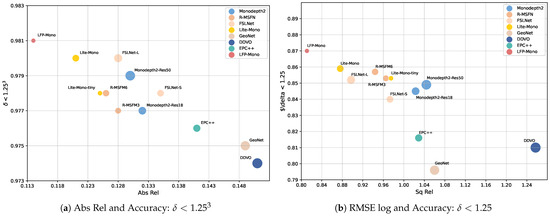
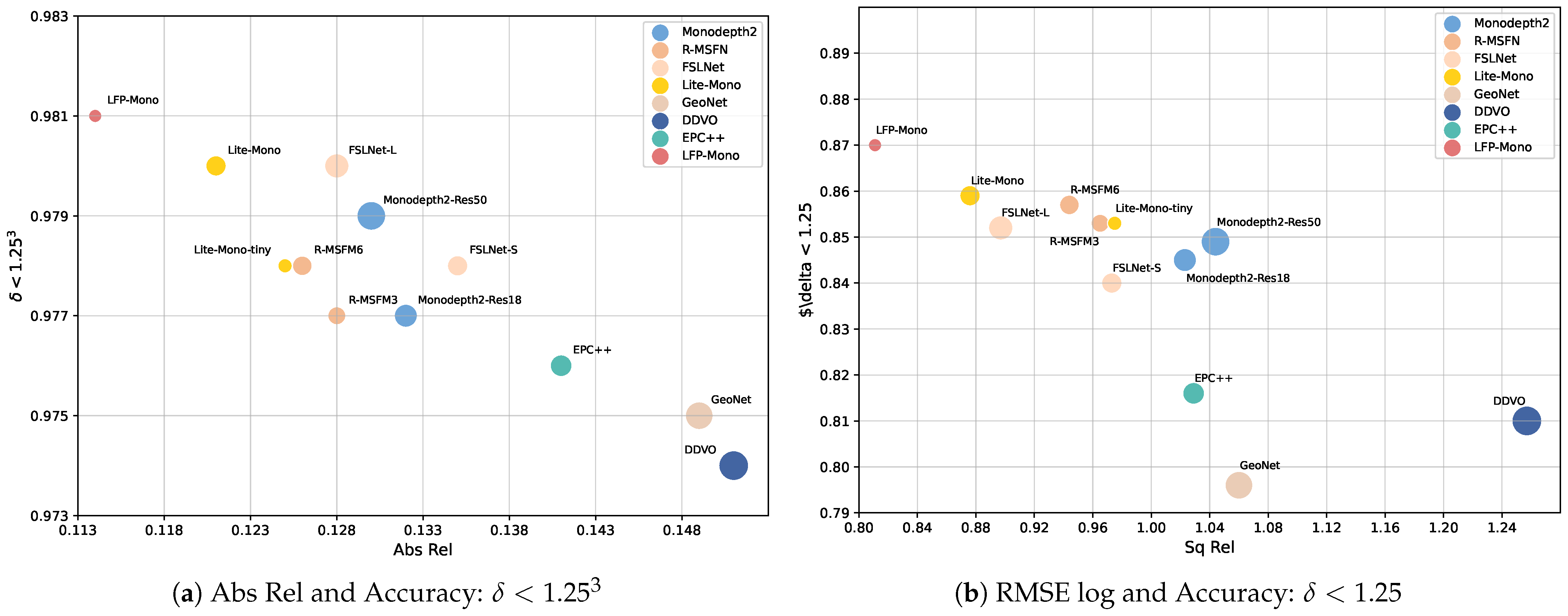
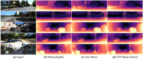
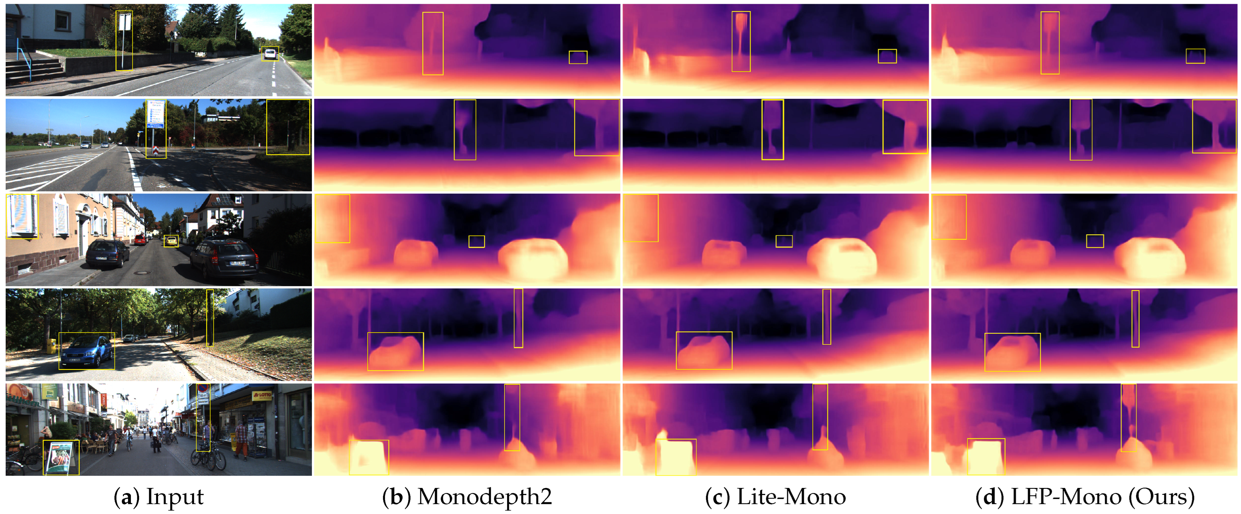
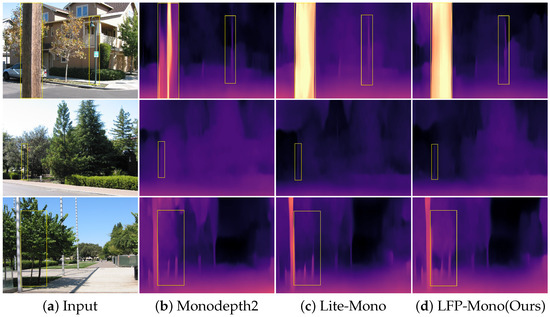
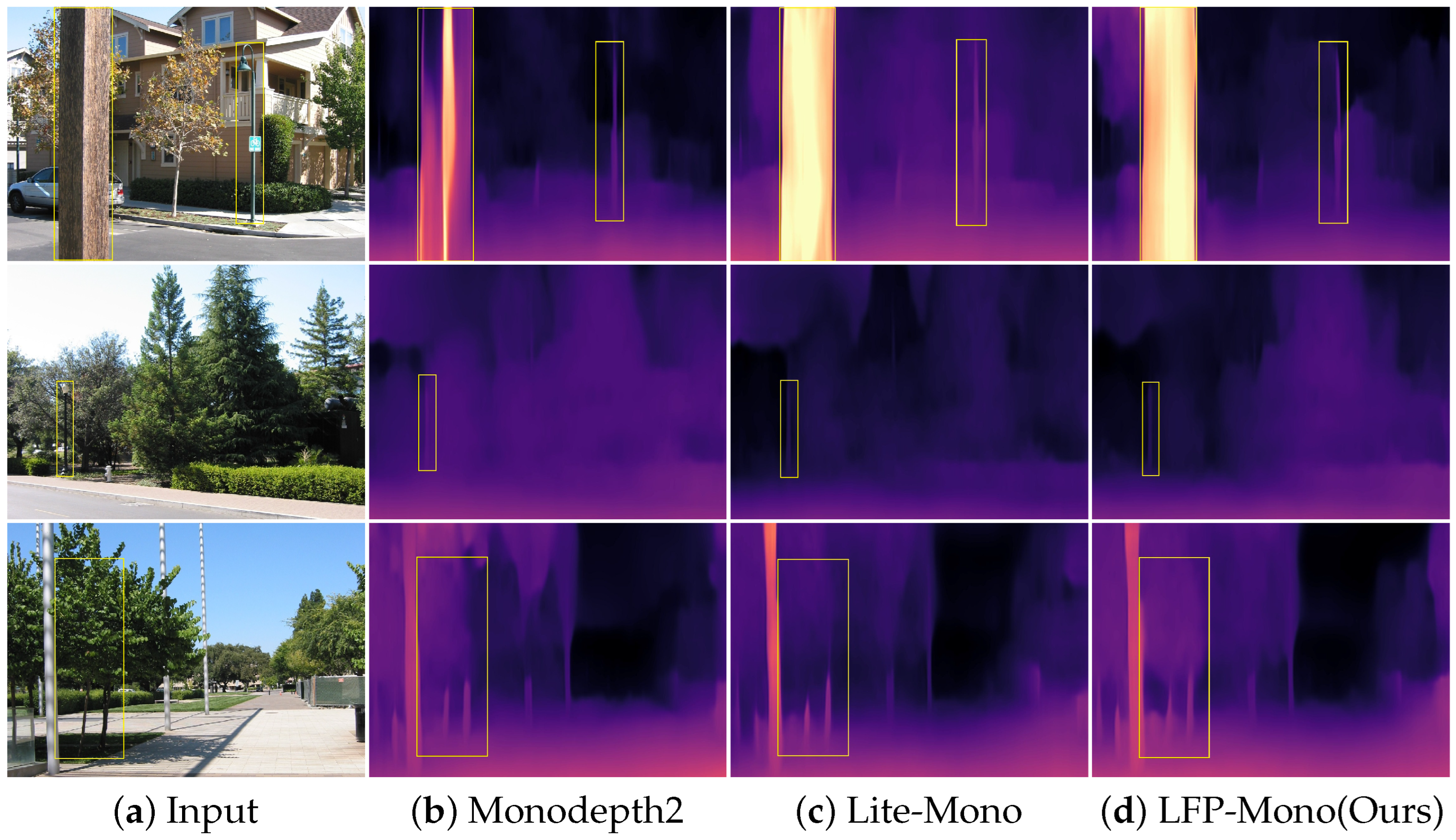
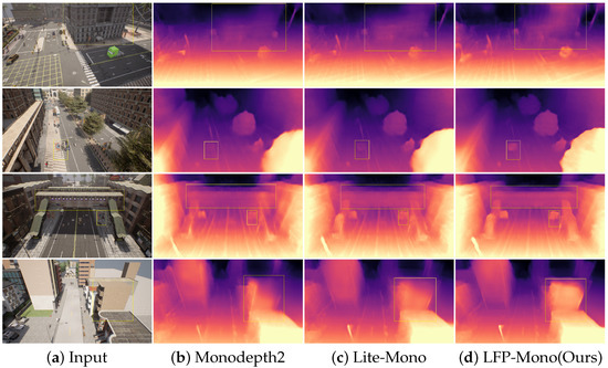
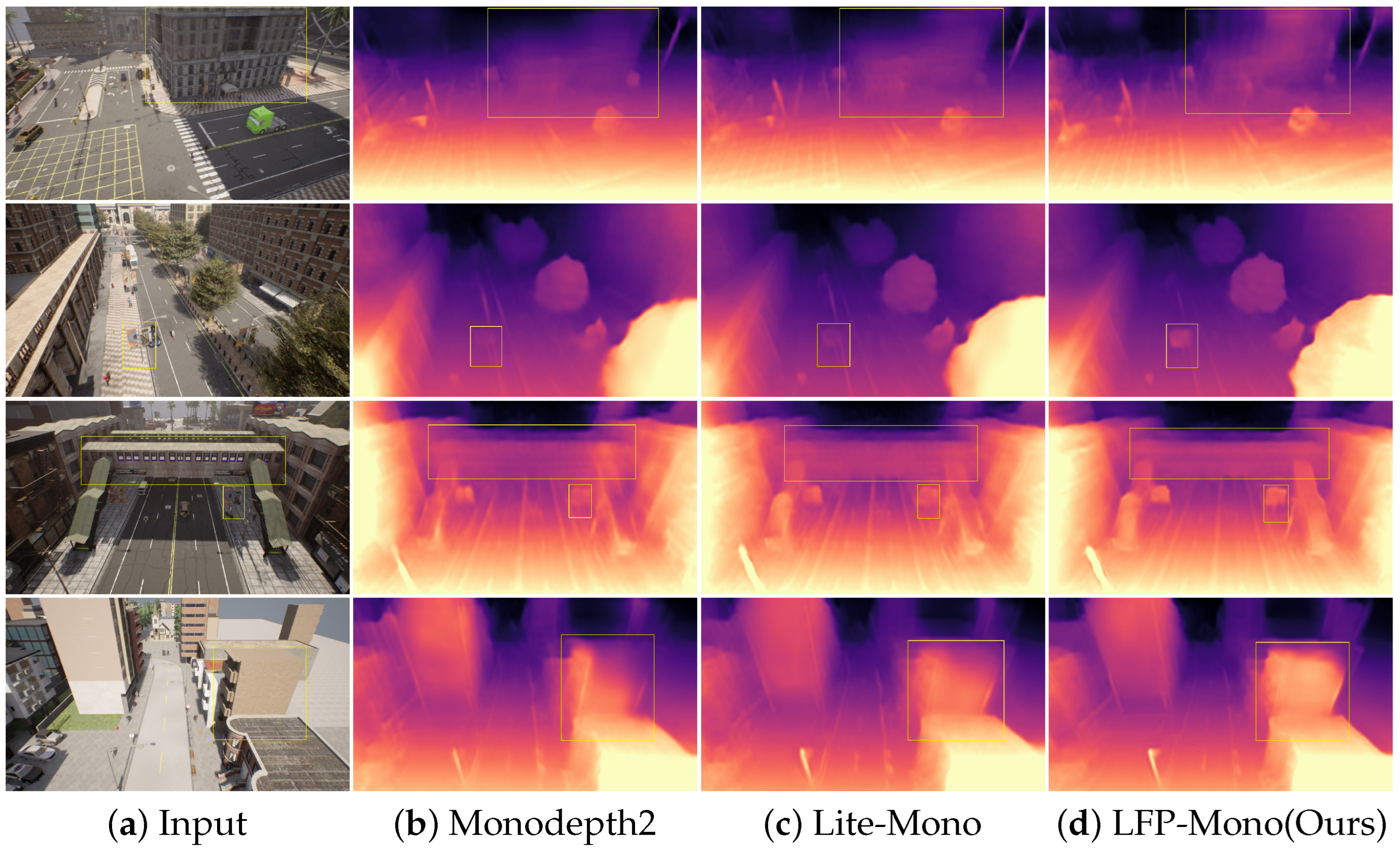
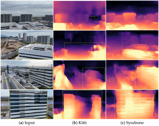
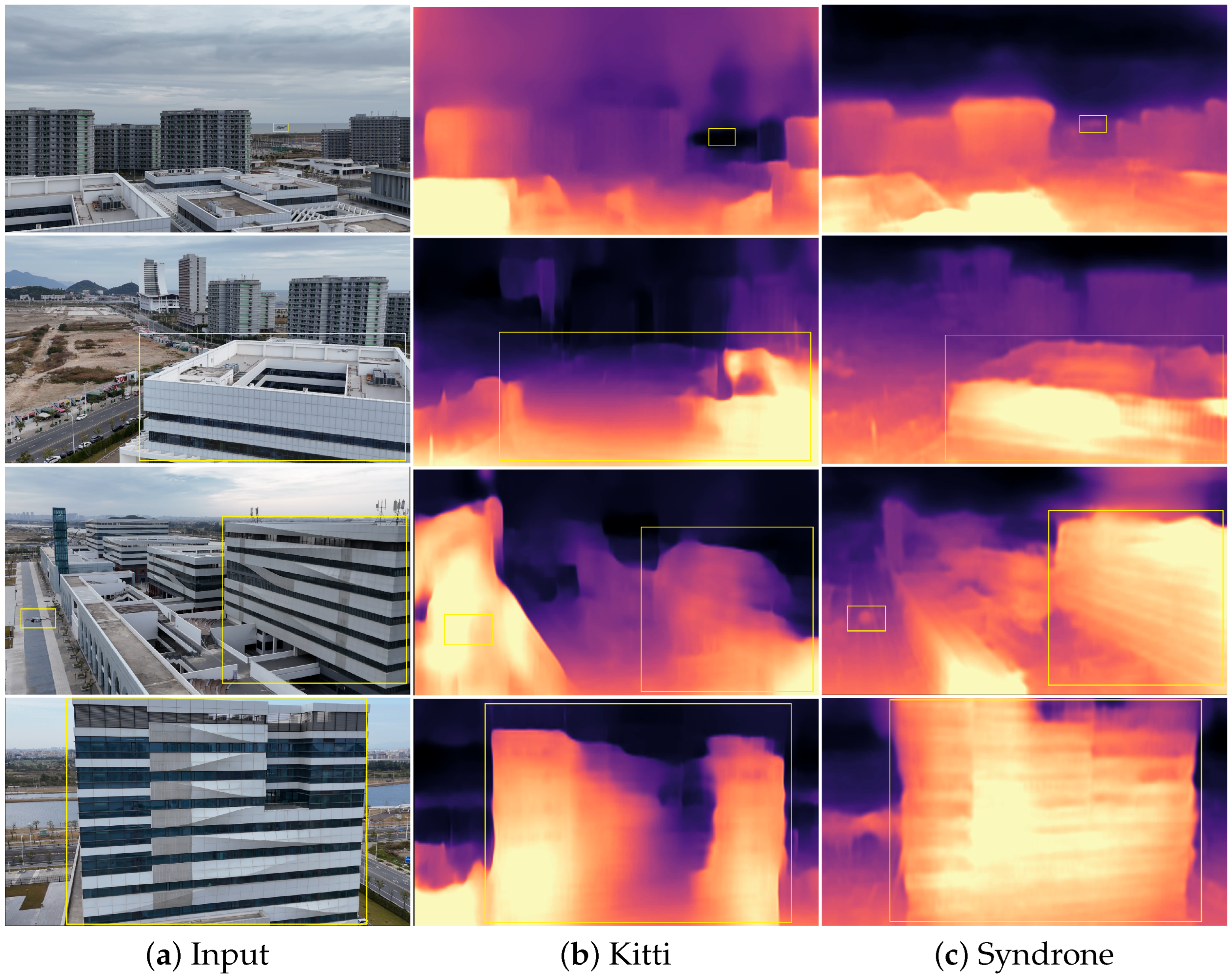

Disclaimer/Publisher’s Note: The statements, opinions and data contained in all publications are solely those of the individual author(s) and contributor(s) and not of MDPI and/or the editor(s). MDPI and/or the editor(s) disclaim responsibility for any injury to people or property resulting from any ideas, methods, instructions or products referred to in the content. |
© 2026 by the authors. Licensee MDPI, Basel, Switzerland. This article is an open access article distributed under the terms and conditions of the Creative Commons Attribution (CC BY) license.