


Highlights
What are the main findings?
- An enhanced spectral feature set (ESFS) was constructed, and two new spectral indices for Pb-contaminated soils, named SPPI-2 and SPPI-3, were developed and incorporated into the ESFS.
- The XGBoost-based satellite hyperspectral mapping model achieved satisfactory performance (RPD = 2.06).
What are the implications of the main findings?
- This study presents new spectral indices for effectively characterizing Pb-contaminated soils and supporting regional-scale soil management.
- This study provides a solution framework for estimating and mapping soil heavy metals, which assists in contamination hotspot identification and promotes environmental sustainability.
Abstract
Satellite hyperspectral remote sensing offers an efficient and cost-effective approach for estimating and mapping soil lead (Pb), thereby supporting pollution identification and environmental sustainability. However, the development of satellite-based spectral estimation models depends on the availability of a robust spectral feature set for soil Pb as input, which is difficult to obtain under field conditions due to interference from moisture, particle size, and light scattering. To address this issue, controlled spectral experiments were conducted on laboratory-prepared soil samples with varying Pb contamination levels. The spectral characteristics associated with Pb contamination were analyzed, and an enhanced spectral feature set (ESFS) was constructed using the successive projections algorithm–Shapley additive explanations method. Two new spectral indices for Pb-contaminated soils, named SPPI-2 and SPPI-3, were developed and incorporated into the ESFS. The ESFS was then applied to satellite hyperspectral data calibrated via direct standardization, with its spectral parameters used as input variables and measured Pb concentrations from field soil samples as the dependent variable. Finally, a satellite-based spectral model for soil Pb estimation was developed using the XGBoost (eXtreme Gradient Boosting) algorithm. Results showed that the spectral parameters in the ESFS included four characteristic bands (R840, R1013, R1215, and R2239) and two newly developed spectral indices (SPPI-2 and SPPI-3). The satellite-based spectral estimation model based on the ESFS and XGBoost algorithm achieved the best performance, with R2 (coefficient of determination) and RPD (ratio of performance to deviation) values of 0.78 and 2.10, respectively, representing a maximum improvement of 164.10% and a minimum improvement of 12.86% (in terms of RPD values) compared to common methods. Hotspot areas of Pb-contaminated soils were mainly found in the eastern part of the abandoned coal mining area, which is associated with improper coal mining and transportation activities. This study presents a satellite hyperspectral framework for effectively estimating the distribution pattern of soil Pb and supporting the regional-scale soil management and environmental sustainability.
1. Introduction
Soil lead (Pb) contamination represents one of the most prevalent forms of soil pollution and a driver of ecological degradation worldwide [1,2]. Such contamination is commonly observed in regions associated with mining activities and intensive industrialization [3,4]. Although Pb occurs naturally in soil parent material as an inherent constituent, anthropogenic activities, including mining, smelting, and transportation, can generate elevated Pb concentrations. These Pb inputs are transferred into the soil through direct discharge and atmospheric deposition, thereby leading to Pb contamination of the soil [5,6]. People living in these areas are exposed to soil Pb, which can enter the body through ingestion, inhalation, and skin contact. Long-term exposure can harm neurocognitive development, especially in children, and can also affect red blood cell production, posing serious health risks [7,8]. Therefore, effective monitoring of the distribution patterns and contamination hotspots of soil Pb is crucial for protecting human health and promoting environmental sustainability.
The satellite hyperspectral technique is effective for estimating the distribution patterns and detecting contamination hotspots of soil Pb in coal mining areas [9,10,11]. Traditionally, the estimation and mapping of soil Pb in coal mining areas relied on an integrated approach involving field soil sampling, laboratory analysis, and geostatistical interpolation [12,13]. Although the method is simple, the labor and time costs are high, and soil Pb monitoring at a regional scale is expensive. Hyperspectral sensors equipped on satellite platforms can collect spectral data over large areas in a short time. By combining machine learning methods, Pb information in the soil can be extracted, enabling large-scale monitoring of soil Pb status and contamination hotspots [9].
A robust set of spectral features used as input variables is essential for developing reliable satellite-based spectral estimation models for soil Pb [14,15]. Usually, spectral features such as characteristic bands are selected from satellite hyperspectral data and then used to explain soil Pb status in spectral models. Satellite hyperspectral data, with its high spectral resolution, provides soil spectral information across many bands, which helps identify absorption features related to soil Pb [16,17]. However, hyperspectral data also contain noise and irrelevant spectral information from environmental factors and other soil properties, not just the spectra of the target soil components [18,19]. Therefore, accurately extracting the spectral features of soil Pb and building an effective spectral feature set are key challenges for developing reliable satellite-based hyperspectral estimation models for soil Pb.
To address this issue, supervised searching methods (such as stepwise regression, correlation coefficient analysis, successive projections algorithm, and competitive adaptive reweighted sampling) were used to select spectral features for soil Pb from high-dimensional hyperspectral data. These selected features were then used as input variables to improve the computational efficiency and accuracy of satellite-based spectral estimation models [20,21,22,23,24]. Furthermore, Pb exists in soil mainly as compounds and is closely associated with adsorptive soil materials, such as organic matter, clay minerals, and iron oxides. Therefore, the spectral features extracted by supervised searching methods indirectly reflect soil Pb, as they are based on the spectral signals of Pb-associated soil components [22,24,25].
Although significant progress has been made in constructing the spectral feature set for soil Pb, two key issues still remain. On one hand, the spectral features of soil Pb and related soil components are often affected or masked by environmental factors such as moisture, particle size, and scattered light. This problem is especially pronounced in satellite hyperspectral data from the complex soil environments found in coal mining areas. As a result, accurately extracting the spectral features of soil Pb and building an efficient spectral feature set remain challenging. On the other hand, spectral indices have clear advantages for characterizing target soil components and improving the accuracy of satellite-based spectral estimation models. They should be an important part of the spectral feature set for soil Pb. However, the current spectral feature sets show clear limitations in this aspect [22,26].
Therefore, in this study, a controlled spectral experiment of laboratory-prepared Pb-contaminated soil was conducted to analyze the response mechanisms between Pb contamination and soil spectra. We then constructed an enhanced spectral feature set (ESFS) by combining characteristic bands related to soil Pb with two newly developed spectral indices for Pb-contaminated soils (SPPI). This feature set can more effectively indicate soil Pb levels. In addition, an advanced machine learning algorithm, eXtreme Gradient Boosting (XGBoost), was used to model the nonlinear relationship between soil Pb and the spectral parameters in the ESFS, thereby building a robust satellite-based spectral estimation model for soil Pb [27].
Spectral indices are powerful tools for indicating soil components, as they enhance spectral information by strategically combining multiple spectral bands and revealing the relationships between them [28,29]. These indices can also serve as covariates during model calibration, thereby improving model accuracy and reliability [30]. For example, Chen et al. [22], Zhang et al. [31], and Santos et al. [32] suggested that the performance of soil spectral estimation models can be improved by including spectral indices as input variables, as these indices are less sensitive to environmental noise. Thus, in this study, an SPPI was developed based on a controlled spectral experiment of laboratory-prepared Pb-contaminated soils and subsequently integrated as a critical component of the ESFS, supporting the development of satellite-based spectral estimation models for soil Pb in coal mining areas.
XGBoost is a machine learning algorithm that can efficiently determine the relationship between spectral parameters within the ESFS and soil Pb concentrations, thus supporting the construction of an accurate satellite-based spectral estimation model [27,33]. This regularized gradient boosting method combines multiple weak predictors iteratively to achieve high accuracy. Its loss function includes regularization terms, which help reduce overfitting and improve model performance [34]. Previous studies have demonstrated its effectiveness in developing spectral estimation models for monitoring soil components such as organic matter, salt, arsenic, pH, and total nitrogen [35,36,37,38]. Overall, combining ESFS with the XGBoost algorithm has great potential to improve the satellite-based spectral estimation of soil Pb.
The study’s objectives were to: (1) develop new spectral indices for Pb-contaminated soils (i.e., SPPI); (2) create an ESFS for characterizing soil Pb status; and (3) build a satellite-based spectral estimation model of soil Pb in coal mining bare-soil areas.
2. Materials and Methods
2.1. Flowchart for Building the Satellite-Based Spectral Estimation Model of Soil Pb
The process of building the satellite-based spectral estimation model of soil Pb is illustrated in Figure 1. First, soil samples with varying Pb contamination levels were prepared in the laboratory, and their spectral data were collected. Next, we identified the characteristic bands of soil Pb and developed an SPPI. These spectral features were combined to create an ESFS for characterizing soil Pb status. Then, an ESFS was constructed from the transformed ZY1-02D satellite hyperspectral data using the direct standardization (DS) algorithm. Subsequently, we used the spectral parameters in the ESFS as independent variables and the measured Pb values of field soil samples as the dependent variable. Finally, a satellite-based spectral estimation model for soil Pb in coal mining bare-soil areas was developed using the XGBoost algorithm.
Figure 1.
Flowchart for building the satellite-based spectral estimation model of soil Pb in coal mining bare-soil areas.
2.2. Study Area and Field Soil Sampling
- (1)
- Study area
An abandoned coal mining area in eastern China was selected as the study area (Figure 2). The study area has a maximum length of 24.2 km and a maximum width of 20.1 km, covering a total area of approximately 335.2 km2, with geographical coordinates ranging from 116°54′26″E to 117°11′2″E and 36°46′3″N to 36°57′21″N. The study area is characterized by the warm temperate semi-humid monsoon climate, with mean annual temperature of 12.8 °C and precipitation of 583.3 mm. The main soil type is Fluvo-aquic soil. Intensive coal mining began in 2007, producing 750,000 metric tons annually until operations ceased completely in 2019 [39].
Figure 2.
Geographic location of the coal mining area and field soil samplings: (a) Location of Jinan City in China; (b) the study area within Jinan City; (c) locations of soil sampling sites and coal mines.
Improper coal mining and coal transport practices have resulted in the dispersion of coal slag and fly ash on soil surfaces [40]. Heavy metal contaminants have entered the soil through hydrologic washout and aeolian transport, leading to the accumulation of soil Pb [41].
- (2)
- Field soil sampling and chemical analysis
Considering factors such as land use, mine distribution, and road conditions, a total of 82 sampling locations were predetermined based on digital maps generated in ArcGIS 10.2 software. Field soil samples were collected during 25–26 February 2023. A handheld GPS was used to navigate to each predetermined sampling location. The distance between any two soil sampling sites is greater than 1.5 km. A multi-point sampling method was employed within a 30-m radius to collect approximately 0.5 kg of soil at a depth of 0–20 cm. The collected soil samples were then sealed in bags and transported to the laboratory for further analysis. Finally, the actual geographic coordinates of each sampling location were recorded again using the handheld GPS device, and environmental conditions, such as temperature and land use, were documented with a smart camera.
In the laboratory, all soil samples were air-dried under natural conditions. We removed small stones, roots, and other impurities, then ground the soil and sieved it through a 0.2 mm mesh. Next, we weighed 0.2 g of soil and transferred the sample to a crucible. After moistening the sample with water, we sequentially added 4 mL HNO3, 1 mL HClO4, and 5 mL HF. The mixture was then digested on a sand bath. After cooling, 5 mL of supernatant was collected into a test tube and diluted with a 1:1 HNO3 solution. Finally, soil Pb concentration was measured using inductively coupled plasma mass spectrometry (ICP-MS) [42].
2.3. Hyperspectral Imagery Acquisition and Preprocessing
2.3.1. Satellite Hyperspectral Imagery Acquisition
ZY1-02D, launched in 2019, is a hyperspectral satellite designed for environmental monitoring and disaster mitigation [43]. The satellite is equipped with two sensors: a panchromatic/multispectral imager and a hyperspectral sensor [44]. The hyperspectral sensor covers the 400–2500 nm range with 166 spectral bands, including 76 bands with the spectral resolution of 10 nm in the 400–1000 nm range and 90 bands with a spectral resolution of 20 nm in the 1000–2500 nm range [45]. The spatial resolution of the hyperspectral imagery is 30 m. ZY1-02D satellite hyperspectral imagery was downloaded from the China Center for Resources Satellite Data and Application (https://data.cresda.cn). The acquisition date of the satellite hyperspectral imagery was 1 March 2023, which is close to the time when the field soil samples were collected.
2.3.2. Extracting the Bare Soil Areas from the Hyperspectral Imagery
The preprocessing for ZY1-02D hyperspectral imagery included three steps [44,46]: First, radiometric calibration and atmospheric correction were conducted using standard modules in ENVI 5.6 software. Next, geometric correction and orthorectification were performed using Landsat 8 reference images and 250 m DEM data. Finally, noisy bands in the spectral ranges of 400–422 nm and 2451–2500 nm were removed, leaving 148 spectral bands for spectral estimation modeling.
Additionally, the non-bare soil regions in the ZY1-02D hyperspectral images were excluded [47,48]. Based on the results of preliminary experiments and previous studies [15,28], regions with NDVI values between 0 and 0.5 were classified as bare soil. A binary image approach was used to mask the non-bare soil regions and extract the bare soil areas. The accuracy of the extracted bare soil areas was assessed using Google Maps (Version 10.15) through random sampling methods, achieving an overall accuracy of 95%. The masking of bare soil areas in satellite hyperspectral imagery is reliable.
2.4. Building the Enhanced Spectral Features Set (ESFS)
2.4.1. Laboratory Preparation of Pb-Contaminated Soil Samples
- (1)
- Preparation of the Pb-contaminated soil samples
A total of 80 soil samples with different Pb contamination levels were prepared in the laboratory. The soil materials associated with the Pb such as soil organic matter, clay, and iron oxides, were set as control variables. This controlled laboratory experiment strongly supports the analysis of the spectral mechanisms of Pb-contaminated soils and the development of spectral feature sets [47,49].
The procedures for preparing Pb-contaminated soil samples are as follows (as shown in Figure 3): First, 10 kg of clean soil was collected from the coal mining area and air-dried under natural conditions (approximately 25 °C). Stones, twigs, and roots were removed, and the soil was sieved through a 1 mm mesh. Next, 50 g of soil was weighed into beakers (labeled D01–D80), and Pb(NO3)2 solutions (50 μg/mL or 1 mg/mL) were added. The volume of the Pb(NO3)2 solution used is provided in Table S1. Ultrapure water was added to cover the soil, and the mixture was thoroughly stirred with glass rods. The prepared Pb-contaminated soil samples were air-dried in a fume hood, ground again, and sieved through a 0.2 mm mesh. Each sample was divided into two parts: one for hyperspectral measurement and the other for soil Pb determination. All steps were conducted in accordance with strict safety protocols, including proper ventilation, the use of personal protective equipment (respirators, gloves, and goggles), and appropriate waste disposal [50].
Figure 3.
Illustrations of the laboratory preparation of Pb-contaminated soil samples: (a) clean soils collected from the study area; (b) Pb(NO3)2 solutions with a mass fraction of 50 μg/mL or 1 mg/mL; (c,d) steps in the laboratory preparation of Pb-contaminated soil samples; (e) laboratory-prepared soil samples with different levels of Pb contamination.
- (2)
- Statistical characteristics of soil Pb concentrations in laboratory-prepared soil samples
The statistical characteristics of Pb concentrations in the laboratory-prepared soil samples are shown in Table 1. Pb concentrations ranged from 16.20 to 474.98 mg/kg, with both the mean and median values being 105.55 mg/kg, which indicates that the dataset follows a normal distribution. The coefficient of variation for the laboratory-prepared soil sample dataset is 1.14, indicating high variability [20]. The kurtosis and skewness values were 2.08 and 1.81, respectively, indicating a right-skewed distribution. The background value of soil Pb in the coal mining area is 21.40 mg/kg, which is significantly lower than the range of Pb concentrations observed in the laboratory-prepared soil samples [51].
Table 1.
Descriptive statistics of Pb concentrations in laboratory-prepared soil samples/(mg/kg).
2.4.2. Spectral Measurement
- (1)
- Imaging spectral measurement
The HySpex hyperspectral imaging system (Norsk Elektro Optikk, NEO, Oslo, Norway) was used to measure the spectral reflectance of the laboratory-prepared Pb-contaminated soil samples [52]. The HySpex system provided spectral measurements in the range of 400–2500 nm across 472 spectral bands. The spectral range of 400–1000 nm contains 186 bands with a resolution of 3 nm, while the spectral range of 1000–2500 nm includes 286 bands with a resolution of 5 nm.
Interfering factors such as scattered light, moisture, and particle size were excluded during the laboratory spectral measurements of soil samples. 15 g of Pb-contaminated soil was evenly spread onto black trays, which were then placed on the stage. In addition, a white reference panel was placed on the stage. Twelve 50 W halogen lamps were arranged strategically in the darkroom as the light source. Finally, the HySpex system was activated, and each soil sample was measured three times.
- (2)
- Spectral pretreatment
Spectral pretreatment was conducted to obtain representative spectra of the laboratory-prepared Pb-contaminated soil samples [53]. First, the raw DN values of the imaging spectral data were converted into spectral reflectance. Next, noisy data, such as that at the image edges, was removed. The spectral range of 400–447 nm was excluded due to its low signal-to-noise ratio. In addition, the spectral regions affected by water absorption (1300–1500 nm and 1800–2000 nm) were eliminated. After preprocessing, a total of 374 spectral bands were retained. Finally, 20 random pixels were selected, and their average values were calculated to represent the spectra of each soil sample.
where Rs represents the spectral reflectance of the soil samples, DNs and DNw represent the digital values of the soil samples and the white reference panel, respectively. Rw represents the calibration coefficient of the spectral reflectance provided by NEO Company.
Rs = (DNs/DNw) × Rw
2.4.3. Spectral Transformation
Spectral transformations were performed to enhance the spectral features of Pb-contaminated soil and reduce random noise [54]. Eleven methods were applied to transform the soil spectral data: mean centering (CT), first derivative (D1), second derivative (D2), detrending (DT), max-min normalization (MMS), Savitzky–Golay smoothing (SG) (The window size and polynomial order were defined as 5 and 2, respectively), standard normal variate (SNV), square root transformation (SQ), standardization (SS), reciprocal transformation (RE), and moving average smoothing (MA). Detailed descriptions of these methods are available in references [55,56,57,58].
2.4.4. Characteristic Bands Selection
Identifying the characteristic bands of soil Pb is crucial for constructing SPPI and for the development of ESFS. First, the optimal spectral transformation method was determined based on the lowest RMSECV (Root mean square error after five-fold cross-validation), using the successive projections algorithm (SPA). SPA is a forward cycling feature selection algorithm where feature subsets with minimal collinearity are selected using projection methods in vector space [59]. Based on the 11 transformed spectral data, vectors with higher projections in the vector space become new starting vectors in each iteration of the SPA method. Through regression calculations, the RMSECV can be obtained. The spectral data with the minimum RMSECV value is regarded as the optimal spectral transformation method. Next, the importance of spectral bands was analyzed using the Shapley Additive Explanations (SHAP) algorithm, and the characteristic bands of soil Pb were identified. SHAP is a method used to quantitatively assess the explanatory contribution of spectral bands to target soil properties. The contribution of each spectral band to the estimation model is computed to evaluate the importance of individual bands and to identify the characteristic bands for soil Pb [60].
The characteristic bands of soil Pb were selected and are shown in Figure 4. The RMSECV values of the transformed spectral data followed the following increasing order: MMS (lowest), SQ, SS, SNV, MA, CT, D1, DT, SG, RE, and D2 (highest). Among these methods, MMS was identified as the most effective approach for spectral transformation. Four characteristic bands were identified: R840, R1013, R1215, and R2239.
Figure 4.
RMSECV values of various transformed spectra (a) and SHAP values of spectral bands in MMS-transformed data (b). RMSECV stands for root mean square error, SHAP stands for Shapley additive explanations, and MMS denotes the max-min normalization transformation method.
2.4.5. SPPI Construction
- (1)
- Key parameters and formulas
Three characteristic bands were defined as spectral points, namely point A (λ840, R840), point B (λ1013, R1013), and point C (λ1215, R1215), which are located in the increasing part of the spectral curve (as indicated in Figure 5). In contrast, spectral point D (λ2239, R2239) occurs at a distinct reflectance peak. Together, these four spectral points characterize the reflectance and absorption features of the soil MMS-transformed spectral curve.
Figure 5.
Illustrations of the new spectral indices for Pb-contaminated soil (SPPI-1, SPPI-2, and SPPI-3).
The changes in these four spectral points reflect the shapes and variations in the spectral curves of Pb-contaminated soils, and also indicate the contamination levels of the soil samples. Therefore, points A, B, C, and D form the foundation for developing the SPPI. Additionally, the triangular spectral index effectively captures the morphology and variations in spectral curves by combining multiple spectral bands [61]. Here, we developed the SPPI as follows:
where λ represents the wavelengths of the spectral bands, and R indicates the soil reflectance values derived from the MMS-transformed spectral data.
- (2)
- Optimal SPPIs
The Pearson correlation coefficients (CC) of the spectral parameters (including SPPI-1, SPPI-2, SPPI-3, and all single bands) are shown in Figure 6. Within the spectral range of 560–1020 nm, the CC values of the spectral bands increase progressively with increasing wavelength, reaching a maximum CC value of 0.46 at R1020. The CC values of the characteristic bands R840 and R1013 are 0.41 and 0.44, respectively. In addition, the CC value of spectral band R2100 (0.30) was found to be the lowest within the spectral range of 2000–2450 nm, while the CC values of the neighboring spectral bands are relatively high. The CC value of the characteristic band R2239 is 0.42. In contrast, the CC values for SPPI-1, SPPI-2, and SPPI-3 are 0.61, 0.94, and 0.98, respectively, indicating a strong correlation with soil Pb concentrations. Consequently, SPPI-2 and SPPI-3 were identified as the optimal spectral indices for Pb-contaminated soil and were selected to constitute the ESFS.
Figure 6.
Pearson correlation coefficients (CC) of spectral bands (left) and spectral indices for Pb-contaminated soil (SPPI-1, SPPI-2, and SPPI-3) (right).
2.5. Transferring the ESFS from Laboratory to Satellite
Narrowing the differences between laboratory and satellite spectra is essential for transferring the ESFS from laboratory to satellite data. First, band removal and resampling methods were integrated to achieve consistency in the number of spectral bands (n = 148) and wavelength positions between the satellite and laboratory data. Noted that the characteristic bands need to be retained during the dimensionality reduction of the laboratory spectral data. Next, the direct standardization (DS) algorithm was applied to establish the relationship between laboratory and satellite spectra, and to minimize their differences through spectral transformation [47,62,63]. DS was originally developed for spectral model transfer between instruments with varying operating conditions [64]. Ji et al. [65] further expanded the application of the DS method to link laboratory and field soil spectra, effectively removing the influence of moisture from field soil spectra. In this study, the DS-based transformation method was employed to construct the ESFS using ZY1-02D hyperspectral data. The equation for the DS algorithm is given below:
where is ZY1-02D satellite hyperspectral data, represents the laboratory hyperspectral data, and B and E are the transformation matrix and residual matrix, respectively. Detailed information can be found in references [47,62,64,66]. The DS method was performed using Python 3.8 software.
2.6. XGBoost Algorithm
XGBoost is an advanced machine learning algorithm that combines gradient boosting with regularization to reduce overfitting while improving the generalization ability of models [27,33]. The XGBoost model works by iteratively building multiple decision trees (serving as weak predictors), each trained to correct the errors of the previous ones. During the training process, XGBoost adds regularization terms to the loss function to control model complexity and enhance robustness [34]. The target model consists of k decision trees, each with optimized weights at its leaf nodes, and makes predictions by summing all trees’ weighted outputs to create a complete gradient-boosted decision tree [35,37,38]. The XGBoost model can be expressed as follows:
where L(θ) represents the loss function, denotes the regularization term, and represent the measured and predicted values of the ith sample, respectively, γ is the penalty cost for new leaf nodes, T is the total number of leaf nodes, λ is the regularization parameter, and is the weight of the jth leaf node.
The hyperparameter configuration was optimized to obtain a robust XGBoost model. The number of estimators was chosen from a range of 50 to 300. The maximum tree depth values ranged from 3 to 10. The value ranges for learning rate, subsample ratio, column sample by tree ratio, and gamma values were (0.01 to 0.2), (0.6 to 0.8), (0.6 to 0.8), and (0 to 0.6) respectively. The optimal configuration of hyperparameters was obtained using cross-validation and grid search methods, indicating that the model achieved an optimal balance between accuracy, computational cost, and time efficiency [67].
Additionally, an early stopping method was implemented to prevent overfitting in the XGBoost model. If the validation error did not decrease over 10 epochs, training would be terminated early, thereby avoiding model overfitting. The early stopping strategy monitors model performance during the training process and automatically stops training to prevent the model from overfitting on the training set, thus improving the model’s generalization ability on unknown sample data and ensuring model accuracy and robustness [68].
2.7. Model Calibration and Evaluation
A total of 82 field soil samples were randomly divided into a calibration set (n = 65) and a validation set (n = 17). The satellite-based spectral estimation model of soil Pb was calibrated using the calibration set [20]. A 10-fold cross-validation method was used to improve the model’s robustness. One-tenth of the stratified samples were randomly selected to validate the model accuracy. The model calculation ended only after all samples had been selected at least once for model calibration and validation. The class proportions of samples were considered in each fold, with representative samples provided in each fold, thereby reducing model bias [67]. The model with the minimum error was considered the optimal model. In addition, the validation set was used only for model evaluation and was kept completely separate from the model calibration [69].
The coefficient of determination (R2), root mean square error (RMSE), and ratio of performance to deviation (RPD) are commonly used metrics to evaluate model performance. R2 indicates how well the predicted values match the measured values, with values closer to 1 representing better accuracy. RMSE measures the magnitude of prediction errors, with smaller values indicating higher precision. RPD is calculated as the ratio of the standard deviation of the validation data to the RMSE. According to Xu et al. [70] and Wang et al. [71], model performance can be classified as poor (RPD < 1.4), moderate (1.4 ≤ RPD < 2), or excellent (RPD ≥ 2). The best satellite-based spectral models are characterized by high R2 and RPD values, along with a low RMSE.
Spectral feature sets composed of different spectral parameters were constructed to evaluate the performance of satellite-based spectral estimation models under varying inputs. Four characteristic bands (R840, R1013, R1215, and R2239) constitute a common spectral feature set (CSFS). The optimal SPPIs were also individually incorporated into the CSFS, generating multiple model inputs (I: R840, R1013, R1215, R2239, and SPPI-1; II: R840, R1013, R1215, R2239, and SPPI-2). The enhanced spectral feature set (ESFS) comprised four characteristic bands and two novel spectral indices (SPPI-1 and SPPI-2). These comparative experiments were conducted to examine the role of SPPIs and ESFS in improving the performance of the XGBoost model.
Additionally, several modeling methods were used to build a satellite-based spectral estimation model for soil Pb, including partial least squares regression (PLSR), artificial neural networks (ANN), support vector machines (SVM), random forests (RF), and extreme learning machine (ELM). Details about these models are available in references [72,73,74,75]. These models were compared with the XGBoost models proposed in this study to evaluate their accuracy and robustness. Furthermore, the tuning of hyperparameters and the integration of grid search method to achieve optimal model performance. The configuration of hyperparameter combinations and the search space are shown in Table 2.
Table 2.
Configuration of hyperparameter combinations and search space of the compared models.
3. Results and Analysis
3.1. Descriptive Statistical Characteristics of Pb Concentrations in Field Soil Samples
The descriptive statistics of soil Pb concentrations in the total sample set, calibration set, and validation set are shown in Figure 7. The Pb concentrations in the total set range from 17.40 to 29.40 mg/kg, with an average of 22.58 mg/kg. Both the calibration and validation sets have similar ranges of soil Pb concentrations compared to the total sample set. In addition, the mean and median values in the total, calibration, and validation sets are in close agreement, indicating that the sample datasets are approximately normally distributed [76]. The descriptive statistics of the three sample sets demonstrate that the sample data are suitable for spectral model calibration and validation.
Figure 7.
Descriptive statistical characteristics of Pb concentrations in the total sample set, calibration sample set, and validation set.
Additionally, the maximum Pb concentration in soils in the total sample set was 29.40 mg/kg, which is about 1.37 times higher than the background value [51] of 21.40 mg/kg. Furthermore, approximately 68.29% of the samples exceeded the background value, indicating moderate Pb contamination in soils in the coal mining area. Therefore, monitoring the soil Pb status and contamination of hotspot areas is essential to promote environmental sustainability and protect human health in the coal mining area.
3.2. Spectral Characteristics of Laboratory, Satellite, and DS-Transformed Satellite Spectra
The laboratory spectra, raw satellite spectra, and DS-transformed satellite spectra are shown in Figure 8a. The reflectance values of the satellite spectra (around 0.2) are much lower than those of the laboratory spectra (around 0.4), indicating that the environmental effects on the satellite spectra are significant. After DS transformation, the satellite spectra show a significant increase in reflectance, closely matching the laboratory spectra. The environmental effect on the satellite spectra is reduced, and the difference between the laboratory and satellite spectra is narrowed, which supports the construction of an ESFS based on ZY1-02D satellite hyperspectral data.
Figure 8.
Soil spectral curves from laboratory, satellite, and DS-based transformed satellite data (a). Spectral curves of laboratory-prepared soil samples with different Pb concentrations (b).
Figure 8b shows the spectral curves of laboratory-prepared soil samples with different Pb concentrations. The reflectance values decrease as the Pb concentration increases, indicating a negative correlation. The soil sample with a Pb concentration of 46.20 mg/kg has significantly higher reflectance than samples with concentrations of 95.20 mg/kg, 275.13 mg/kg, 435.02 mg/kg, and 455.00 mg/kg. Additionally, the spectral curves of soil samples with different Pb levels show an overall increase in reflectance across the 400–2100 nm range. This increase is most pronounced between 400 and 800 nm, after which the rate of increase gradually slows. Two absorption valleys are removed near 1400 nm and 1900 nm, which may be due to soil moisture [77]. Reflectance peaks appear near 1000 nm and 2200 nm, possibly related to the presence of clay minerals, organic matter, and iron oxides in the soil [23,78,79].
Additionally, three sensitive spectral ranges for soil Pb are highlighted in Figure 8b, specifically at 800–1300 nm, 1500–1800 nm, and 2100–2450 nm. Within these ranges, there is a clear negative correlation between soil Pb and spectral reflectance. Overall, data analysis of laboratory spectra, satellite spectra, and DS-transformed satellite spectra supports the identification of characteristic bands and the development of the SPPI. The observed negative relationship between Pb concentrations and spectral reflectance provides a solid foundation for constructing satellite-based spectral estimation models of soil Pb.
3.3. Comparison of Satellite-Based Spectral Estimation Models for Soil Pb
Satellite-based spectral estimation models of soil Pb were developed using the XGBoost algorithm with two spectral feature sets: CSFS (R840, R1013, R1215, R2239) and ESFS (R840, R1013, R1215, R2239, SPPI-2, and SPPI-3). The validation results of the models are shown in Figure 9. Model IV (using ESFS as input variables) (Figure 9d) shows the best performance, with R2, RMSE, and RPD values of 0.78, 1.11 mg/kg, and 2.10, respectively. The deviation between measured and estimated Pb values from Model IV was minimal. Model II (Figure 9b) was calibrated using a combination of CSFS and SPPI-2 as input variables, and it also showed good performance (R2 = 0.73, RPD = 1.90). Furthermore, Models III (Figure 9c) and I (Figure 9a) showed moderate accuracy, with RPD values of 1.77 and 1.61, respectively. Overall, the XGBoost algorithm combined with ESFS produced an accurate satellite-based spectral model for soil Pb.
Figure 9.
Scatter plots of measured vs. estimated Pb values in soils using satellite-based spectral estimation models based on the common spectral feature set (CSFS) and enhanced spectral feature set (ESFS). SPPI-2 and SPPI-3 represent the newly developed spectral indices for Pb-contaminated soils. The unit of RMSE is mg/kg.
3.4. Soil Pb Maps
To assess the applicability of the satellite-based spectral estimation model of soil Pb (Model IV, as indicated in Figure 9d), the model was applied to coal mining bare-soil areas using the DS-transformed satellite hyperspectral data. The estimated soil Pb values and their distribution map are shown in Figure 10. Contamination hotspots were mainly found in the eastern part of the coal mining area, while soils in the central and western regions were relatively clean. Most abandoned mines are located in the southeast of the coal mining area (as indicated in Figure 2), which may contribute to soil Pb contamination through the transfer of coal slag and coal ash from the historical mining activities [80,81]. In addition, contamination hotspots were also observed in roadside soils, likely due to inappropriate coal transportation activities.
Figure 10.
Distribution map of soil Pb concentration in a coal mining bare-soil area in China.
Based on the reference background value of soil Pb (21.40 mg/kg) [51], approximately 36.5% of soils in the coal mining bare-soil area are classified as Pb-contaminated, while the remaining 63.5% are regarded as clean. Pb-contaminated soils are mainly distributed in the east and south of the coal mining area, while clean soils are primarily found in the west and north. The estimated Pb concentrations range from 14.25 to 35.66 mg/kg, which are basically consistent with the measured soil Pb concentrations (17.40–29.40 mg/kg). Mapping results indicate that the satellite-based spectral estimation model for soil Pb (Model IV) developed in this study is reliable.
3.5. Uncertainty in the Soil Pb Mapping
The satellite-based spectral estimation model of soil Pb (Model IV, as indicated in Figure 9d) was iterated 50 times and its standard deviation was calculated to assess the uncertainty of soil Pb mapping. The uncertainty of soil Pb mapping using the satellite-based spectral estimation model is shown in Figure 11. The uncertainty of soil Pb mapping ranges from 0 to 0.5 mg/kg, with an average of 0.44 mg/kg. The eastern region of the study area exhibits higher uncertainty than the western region, indicating that soils in the eastern area have stronger spatial heterogeneity and more complex environmental conditions, thereby increasing the uncertainty of soil Pb mapping. In the future, incorporating appropriate environmental covariates into satellite-based spectral modeling or increasing the number of field samples collected in specific areas may reduce the uncertainty of soil Pb mapping [70].
Figure 11.
Uncertainty in the soil Pb mapping (the standard deviation represents the average results of estimated Pb values from 50 iterations of the model).
4. Discussion
In this study, we developed an enhanced spectral feature set (i.e., ESFS) derived from a controlled spectral experiment with laboratory-prepared Pb-contaminated soil samples. This ESFS comprises four characteristic bands (R840, R1013, R1215, and R2239) and two newly developed spectral indices (SPPI-2, SPPI-3), which effectively characterize soil Pb status in coal mining areas. Then, the ESFS was adapted for satellite application by applying a DS-based transformation to satellite hyperspectral data. The spectral parameters from the ESFS were used as independent variables, and the measured Pb concentrations from field soil samples were used as dependent variables. The satellite-based spectral estimation model for soil Pb was constructed using the XGBoost algorithm.
A controlled spectral measurement experiment using laboratory-prepared Pb-contaminated soil samples is recommended for understanding the spectral mechanisms of Pb-contaminated soils and for identifying the spectral features of soil Pb. Common methods for extracting spectral features, such as supervised searching methods (e.g., competitive adaptive reweighted sampling, genetic algorithms, and successive projections algorithm), were applied based on a repeated iterative fitting approach [20,44,82]. A statistical result of the selected bands was used in CSFS. However, environmental factors such as moisture, particle size, and scattered light were not considered during feature extraction [65,83]. As a result, the CSFS may only be suitable under a given environmental condition. The CSFS faces challenges in accurately characterizing soil Pb in areas where soil environments change significantly, especially in coal mining regions. Therefore, soil Pb contamination was prepared and a controlled spectral measurement experiment was conducted, with interfering factors such as moisture, particle size, scattered light, and soil background properties excluded. The experimental data supported understanding the spectral response of Pb-contaminated soils, and the new spectral indices for Pb-contaminated soils (SPPI-2 and SPPI-3) were developed, leading to the establishment of the ESFS.
The new spectral indices for Pb-contaminated soil, SPPI-2 and SPPI-3, are a crucial part of the ESFS, which can effectively indicate the Pb contamination status in soils. The spectral indices SPPI-2 and SPPI-3 were calculated using tangent angles from four characteristic bands (R840, R1013, R1215, and R2239). The spectral features of Pb-contaminated soils, identified using the tangent method, were further enhanced by strategically combining these features and by analyzing the interrelationships among key spectral bands [84]. In soil, Pb exists in forms bound to active substances (such as organic matter, iron oxides, and clay) adsorbed in the soil. Therefore, the spectral features displayed by Pb are closely linked to these spectrally active soil components [85,86]. Sun et al. [86] suggested that clay in soil exhibits spectral features around 2200 nm due to the influence of soil clay minerals. Li et al. [87] indicated that spectral bands near 1000 nm, 1050 nm, 1300 nm, 2200 nm, and 2260 nm correlate with certain functional groups in soil organic matter. The spectral ranges of 870 nm and 1000–1100 nm are sensitive to iron oxides in soil, but are also influenced by soil organic matter [23,88,89]. In addition, Wang et al. [9] reported that the spectral ranges of 375–800, 900–1200, 1300–1450, 1700–2080, 2150, and 2200–2400 nm are sensitive spectral regions for heavy metals in soil. The characteristic bands selected in this study and the newly developed spectral indices (SPPI-2 and SPPI-3) further confirm existing spectral mechanisms of lead-contaminated soils. In addition, SPPI-2 and SPPI-3 highlight the global changes in the spectral curves of Pb-contaminated soils, while single spectral bands represent localized spectral features that may be masked or affected by environmental factors or other soil components.
Additionally, common spectral indices of soils were constructed in the comparative experiment, and showed unsatisfactory performance in characterizing the soil Pb status. Common spectral indices such as the difference spectral index (DI), ratio spectral index (RI), and normalized difference spectral index (NDI) were developed [31,90], and their CC values are shown in Figure 12. The absolute CC values for the common spectral indices range from 0 to 0.36, which are lower than those of SPPI-2 (0.53) and SPPI-3 (0.62). These differences suggest that common spectral indices are ineffective for indicating soil Pb status in coal mining bare-soil areas, likely due to the complex soil environment and influences from other soil components.
Figure 12.
Pearson correlation coefficients (CC) of common spectral indices: (a) Difference spectral index (DI); (b) Ratio spectral index (RI); (c) Normalized difference spectral index (NDI).
The satellite-based spectral estimation model of soil Pb based on the ESFS and XGBoost (Model IV, shown in Figure 9) performed better than other commonly used models. Several models, such as PLSR, ANN, ELM, SVM, and RF, were constructed [64,69,72,73,74], and their performance metrics are listed in Table 3. The RF model achieved the highest accuracy among the common models, with an R2 of 0.70 and an RPD of 1.83. The RPD value of the RF model was still about 12.86% lower than that of model IV. The ELM model ranked second for soil Pb spectral estimation (RPD = 1.70), while PLSR, ANN, and SVM had relatively lower accuracy (RPD ranging from 0.78 to 1.62). The Model IV, based on the ESFS and XGBoost algorithm, demonstrated the best accuracy and reliability, improving the minimum accuracy for soil Pb spectral estimation by 12.86% compared to the common models.
Table 3.
Comparison of satellite-based spectral estimation models of soil Pb constructed using common methods.
In addition, we acknowledge that improvements in satellite-based spectral estimation of soil Pb rely on the construction of a robust spectral feature set, the use of advanced machine learning models, and the optimization of the methodological framework. Clearly, the above improvements and optimizations are developed within the existing theoretical framework of soil hyperspectral estimation [9]. In future work, further efforts could focus on developing new theoretical frameworks to achieve greater improvements in the satellite-based spectral estimation and mapping of soil heavy metals.
The DS-based transformation method plays an important role in establishing the ESFS using satellite hyperspectral data. Differences between satellite and laboratory spectra, such as spectral resolution and reflectance values, are commonly observed. These differences are mainly caused by environmental factors and differences in spectrometer sensors. It should be noted that the ESFS was originally developed using laboratory spectra. DS is commonly used for transferring data or models between different spectrometers under varying measurement conditions, and its reliability has been demonstrated in studies by Ji et al. [62] and Xu et al. [45]. Therefore, in this study, the DS method was used to transform the satellite hyperspectral data, allowing the ESFS to be transferred from laboratory to satellite data and ensuring its applicability to the satellite data.
The sample size and representativeness of field-collected soil samples play an important role in the performance of satellite-based spectral estimation models. In this study, before field sampling, land use, soil type, mine distribution, and road conditions in the study area were considered to select suitable sampling locations and ensure spatial representativeness of the samples. Additionally, the XGBoost model, which is suitable for different sizes of sample datasets, was used for spectral modeling [37,38]. Results show that when the number of soil samples is less than 50, the XGBoost-based satellite estimation model has low accuracy (R2 < 0.60 and RPD < 1.40) and cannot provide acceptable estimates of soil Pb. When the training sample size increases to more than 60, the model accuracy shows no obvious change and remains stable. These efforts help achieve a balance between model performance and sampling cost. In future work, more soil samples will be collected, and advanced deep learning models will be introduced to further improve the accuracy and reliability of satellite-based spectral estimation models.
To enhance the transferability of the proposed framework (integrating ESFS with the XGBoost model), two aspects merit further consideration. First, noise introduced by factors such as soil moisture in satellite hyperspectral imagery should be carefully assessed and minimized, as this would improve the reliability and accuracy of ESFS in characterizing soil Pb [91]. Second, the development of a reliable XGBoost model relies on representative field soil samples, appropriate hyperparameter tuning, and comprehensive evaluation using independent validation datasets [92]. These efforts are expected to improve the applicability of the proposed framework in other environments, such as agricultural soils or post-conflict areas.
Some limitations exist that will need to be addressed as priorities in future research. We recognize that laboratory spectra of field-collected Pb-contaminated soil samples and laboratory-prepared Pb-contaminated soil samples may have slight differences in shape and absorption features, due to the differences in organic matter, clay, and other soil components between these two types of samples [22]. Although the DS method has been proven effective in reducing differences between the two types of spectra, the spectra of field-collected and laboratory-prepared Pb-contaminated soil samples are quasi-consistent. Moving forward, the mechanisms and sources of spectral differences between field-collected and laboratory-prepared Pb-contaminated soil samples should be investigated and eliminated to improve the applicability of the ESFS. In addition, the combination of cross-validation and grid search achieved an optimal configuration of model hyperparameters. The calibrated model achieved a balance between accuracy and computational cost in this study. In the next step, the integration of automatic hyperparameter search strategies (such as Bayesian optimization) with advanced artificial intelligence models (such as convolutional neural networks and transfer learning) will significantly improve the accuracy and robustness of satellite-based spectral estimation models [68,93].
5. Conclusions
This study proposes a robust satellite-based framework for the estimation and mapping of soil Pb based on the ESFS and the XGBoost model, and its effectiveness has been demonstrated through a case study in a coal mining area. The ESFS was developed using controlled spectral experiment of laboratory-prepared Pb-contaminated soils employing the SPA-SHAP method. Two new spectral indices for Pb-contaminated soils (SPPI-2 and SPPI-3) were constructed. Next, the ESFS was established using DS-transformed satellite hyperspectral data, where the spectral parameters in the ESFS were used as independent variables, and the measured Pb concentrations in field soil samples served as the dependent variable. Finally, a satellite-based spectral estimation model of soil Pb based on the XGBoost algorithm was developed. Results showed that: (1) the spectral parameters in the ESFS included R840, R1013, R1215, R2239, SPPI-2, and SPPI-3; (2) the optimal satellite-based estimation model of soil Pb, calibrated with the XGBoost algorithm and ESFS, achieved R2 and RPD values of 0.78 and 2.10, respectively, which are at least 12.86% higher than those of common models; (3) Pb-contaminated soils were mainly distributed in the eastern part of the coal mining area, which is associated with improper coal mining and transportation activities. The results presented in this study provide an effective approach based on the ESFS and XGBoost model for the satellite estimation and mapping of soil Pb, providing strong support for the monitoring of soil Pb status and Pb-contaminated hotspot areas, and are valuable for soil management and environmental sustainability worldwide.
Supplementary Materials
The following supporting information can be downloaded at: https://www.mdpi.com/article/10.3390/rs18091446/s1, Table S1: Volumes of Pb(NO3)2 solution added for laboratory preparation of Pb-contaminated soil samples.
Author Contributions
Conceptualization, X.X. and Y.W.; methodology, X.D.; software, Z.W.; formal analysis, Q.W.; investigation, X.X.; resources, Q.S.; data curation, X.X. and Y.W.; writing—original draft preparation, X.X.; writing—review and editing, X.D. and J.C.; supervision, J.C.; project administration, J.C.; funding acquisition, J.C. and Q.W. All authors have read and agreed to the published version of the manuscript.
Funding
This work was supported by the Natural Science Foundation of Shandong Province, China (ZR2025QC1023), National Natural Science Foundation of China (42501074), Youth Innovation Team Program of Colleges and Universities in Shandong Province (2022KJ248), and Key Laboratory of Environmental Change and Natural Disaster of the Ministry of Education, Beijing Normal University (2023-KF-12).
Data Availability Statement
Data is available upon request.
Acknowledgments
We thank the Analysis and Test Center, State Key Laboratory of Earth Surface Processes and Hazard Risk Governance, Beijing Normal University, for their support.
Conflicts of Interest
The authors declare no conflicts of interest.
References
- Zhang, M.; Wang, J.; Li, S. Tempo-spatial changes and main anthropogenic influence factors of vegetation fractional coverage in a large-scale opencast coal mine area from 1992 to 2015. J. Clean. Prod. 2019, 232, 940–952. [Google Scholar] [CrossRef] [Scilit]
- Zerizghi, T.; Guo, Q.; Tian, L.; Wei, R.; Zhao, C. An integrated approach to quantify ecological and human health risks of soil heavy metal contamination around coal mining area. Sci. Total Environ. 2022, 814, 152653. [Google Scholar] [CrossRef] [Scilit]
- Liu, X.; Bai, Z.; Shi, H.; Zhou, W.; Liu, X. Heavy metal pollution of soils from coal mines in China. Nat. Hazards 2019, 99, 1163–1177. [Google Scholar] [CrossRef] [Scilit]
- Islam, A.; Jion, M.; Jannat, J.; Varol, M.; Islam, M.; Khan, R.; Idris, A.; Malafaia, G.; Habib, M. Perception and legacy of soil chromium and lead contamination in an operational small-scale coal mining community. Environ. Geochem. Health 2023, 45, 7237–7253. [Google Scholar] [CrossRef] [Scilit] [PubMed]
- Zhu, L.; Zhang, L.; Wang, J.; Lv, J. Combining finite mixture distribution, receptor model, and geostatistical simulation to evaluate heavy metals pollution in soils: Source and spatial pattern. Land Degrad. Dev. 2021, 32, 2105–2115. [Google Scholar] [CrossRef] [Scilit]
- Parzentny, H.R.; Róg, L. Distribution and mode of occurrence of Co, Ni, Cu, Zn, As, Ag, Cd, Sb, Pb in the feed coal, fly ash, slag, in the topsoil and in the roots of trees and undergrowth downwind of three power stations in Poland. Minerals 2021, 11, 133. [Google Scholar] [CrossRef] [Scilit]
- Li, J.; Xu, X.; Lv, J.; Wu, Q.; Ren, M.; Cao, J.; Liu, P. Source apportionment and health risk quantification for heavy metal sources in soils near aluminum-plastic manufacturing facilities in northeast China. Hum. Ecol. Risk Assess. 2020, 26, 2225–2244. [Google Scholar] [CrossRef] [Scilit]
- Collin, M.S.; Venkatraman, S.K.; Vijayakumar, N.; Kanimozhi, V.; Arbaaz, S.M.; Stacey, R.S.; Anusha, J.; Choudhary, R.; Lvov, V.; Tovar, G.I. Bioaccumulation of lead (Pb) and its effects on human: A review. J. Hazard. Mater. Adv. 2022, 7, 100094. [Google Scholar] [CrossRef] [Scilit]
- Wang, Y.; Zou, B.; Chai, L.; Lin, Z.; Feng, H.; Tang, Y.; Tian, R.; Tu, Y.; Zhang, B.; Zou, H. Monitoring of soil heavy metals based on hyperspectral remote sensing: A review. Earth-Sci. Rev. 2024, 254, 104814. [Google Scholar] [CrossRef] [Scilit]
- Mirzaei, M.; Verrelst, J.; Marofi, S.; Abbasi, M.; Azadi, H. Eco-friendly estimation of heavy metal contents in grapevine foliage using in-field hyperspectral data and multivariate analysis. Remote Sens. 2019, 11, 2731. [Google Scholar] [CrossRef] [Scilit]
- Tan, K.; Ma, W.; Chen, L.; Wang, H.; Du, Q.; Du, P.; Yan, B.; Liu, R.; Li, H. Estimating the distribution trend of soil heavy metals in mining area from HyMap airborne hyperspectral imagery based on ensemble learning. J. Hazard. Mater. 2021, 401, 123288. [Google Scholar] [CrossRef] [Scilit] [PubMed]
- Wang, Z.; Chen, X.; Yu, D.; Zhang, L.; Wang, J.; Lv, J. Source apportionment and spatial distribution of potentially toxic elements in soils: A new exploration on receptor and geostatistical models. Sci. Total Environ. 2021, 759, 143428. [Google Scholar] [CrossRef] [Scilit]
- Reza, S.; Baruah, U.; Singh, S.; Das, T. Geostatistical and multivariate analysis of soil heavy metal contamination near coal mining area, Northeastern India. Environ. Earth Sci. 2015, 73, 5425–5433. [Google Scholar] [CrossRef] [Scilit]
- Zhou, M.; Zou, B.; Tu, Y.; Feng, H.; He, C.; Ma, X.; Ning, J. Spectral response feature bands extracted from near standard soil samples for estimating soil Pb in a mining area. Geocarto Int. 2022, 37, 13248–13267. [Google Scholar] [CrossRef] [Scilit]
- Mzid, N.; Castaldi, F.; Tolomio, M.; Pascucci, S.; Casa, R.; Pignatti, S. Evaluation of agricultural bare soil properties retrieval from Landsat 8, Sentinel-2 and PRISMA satellite data. Remote Sens. 2022, 14, 714. [Google Scholar] [CrossRef] [Scilit]
- Canero, F.M.; Rodriguez-Galiano, V.; Chabrillat, S. Evaluating Airborne Hyperspectral Scanner (AHS) for the mapping of soil organic matter and clay in a Mediterranean forest ecosystem. Catena 2025, 252, 108889. [Google Scholar] [CrossRef] [Scilit]
- Zhang, J.; Ding, J.; Tan, J.; Wang, J.; Zhang, Z.; Wang, Z.; Ge, X. Monitoring soil salinization in arid cotton fields using unmanned aerial vehicle hyperspectral imagery. Int. J. Appl. Earth Obs. Geoinf. 2025, 140, 104584. [Google Scholar] [CrossRef] [Scilit]
- Ma, X.; Wang, J.; Zhou, K.; Zhang, W.; Chen, A. Uncertainty in soil elemental prediction using machine learning and hyperspectral remote sensing. J. Hazard. Mater. 2025, 494, 138502. [Google Scholar] [CrossRef] [Scilit] [PubMed]
- Shen, Q.; Shang, K.; Xiao, C.; Tang, H.; Wu, T.; Wang, C. A novel hyperspectral remote sensing estimation model for surface soil texture using AHSI/ZY1-02D satellite image. Int. J. Appl. Earth Obs. Geoinf. 2025, 138, 104453. [Google Scholar] [CrossRef] [Scilit]
- Xu, X.; Ren, M.; Cao, J.; Wu, Q.; Liu, P.; Lv, J. Spectroscopic diagnosis of zinc contaminated soils based on competitive adaptive reweighted sampling algorithm and an improved support vector machine. Spectrosc. Lett. 2019, 53, 86–99. [Google Scholar] [CrossRef] [Scilit]
- Liu, Z.; Lu, Y.; Peng, Y.; Zhao, L.; Wang, G.; Hu, Y. Estimation of soil heavy metal content using hyperspectral data. Remote Sens. 2019, 11, 1464. [Google Scholar] [CrossRef] [Scilit]
- Chen, L.; Lai, J.; Tan, K.; Wang, X.; Chen, Y.; Ding, J. Development of a soil heavy metal estimation method based on a spectral index: Combining fractional-order derivative pretreatment and the absorption mechanism. Sci. Total Environ. 2022, 813, 151882. [Google Scholar] [CrossRef] [Scilit]
- Rossel, R.V.; Behrens, T. Using data mining to model and interpret soil diffuse reflectance spectra. Geoderma 2010, 158, 46–54. [Google Scholar] [CrossRef] [Scilit]
- Sun, W.; Liu, S.; Zhang, X.; Zhu, H. Performance of hyperspectral data in predicting and mapping zinc concentration in soil. Sci. Total Environ. 2022, 824, 153766. [Google Scholar] [CrossRef] [Scilit] [PubMed]
- Nawar, S.; Cipullo, S.; Douglas, R.; Coulon, F.; Mouazen, A. The applicability of spectroscopy methods for estimating potentially toxic elements in soils: State-of-the-art and future trends. Appl. Spectrosc. Rev. 2020, 55, 525–557. [Google Scholar] [CrossRef] [Scilit]
- Lei, H.; Bao, N.; Yu, M.; Cao, Y. Estimating and mapping tailings properties of the largest iron cluster in China for resource potential and reuse: A new perspective from interpretable CNN model and proposed spectral index based on hyperspectral satellite imagery. Int. J. Appl. Earth Obs. Geoinf. 2025, 139, 104512. [Google Scholar] [CrossRef] [Scilit]
- Prakash, A.; Thangaraj, J.; Roy, S.; Srivastav, S.; Mishra, J.K. Model-aware XGBoost method towards optimum performance of flexible distributed Raman amplifier. IEEE Photonics J. 2023, 15, 1–10. [Google Scholar] [CrossRef] [Scilit]
- Xu, X.; Wang, X.; Yang, P.; Meng, Y.; Yu, D.; Li, C. Strategy for mapping soil salt contents during the bare soil period through a satellite image: Optimal calibration set combined with random forest. Catena 2023, 223, 106900. [Google Scholar] [CrossRef] [Scilit]
- Dharumarajan, S.; Lalitha, M.; Kalaiselvi, B.; Kaliraj, S.; Adhikari, K.; Vasundhara, R.; Niranjana, K.; Hegde, R.; Pradeep, C.; Hittanagi, P. Remote sensing of soils: Spectral signatures and spectral indices. In Remote Sensing of Soils; Elsevier: Amsterdam, The Netherlands, 2024; pp. 13–23. [Google Scholar]
- Wang, J.; Ding, J.; Yu, D.; Ma, X.; Zhang, Z.; Ge, X.; Teng, D.; Li, X.; Liang, J.; Lizaga, I.; et al. Capability of Sentinel-2 MSI data for monitoring and mapping of soil salinity in dry and wet seasons in the Ebinur Lake region, Xinjiang, China. Geoderma 2019, 353, 172–187. [Google Scholar] [CrossRef] [Scilit]
- Zhang, Z.; Ding, J.; Wang, J.; Ge, X. Prediction of soil organic matter in northwestern China using fractional-order derivative spectroscopy and modified normalized difference indices. Catena 2020, 185, 104257. [Google Scholar] [CrossRef] [Scilit]
- dos Santos, E.P.; Moreira, M.C.; Fernandes-Filho, E.I.; Demattê, J.A.; dos Santos, U.J.; Moura-Bueno, J.M.; Cruz, R.R.P.; da Silva, D.D.; Sampaio, E.V.d.S.B. Integrating satellite radar vegetation indices and environmental descriptors with visible-infrared soil spectroscopy improved organic carbon prediction in soils of semi-arid Brazil. Geoderma 2025, 457, 117288. [Google Scholar] [CrossRef] [Scilit]
- Wang, S.; Zhou, Y.; You, X.; Wang, B.; Du, L. Quantification of the antagonistic and synergistic effects of Pb2+, Cu2+, and Zn2+ bioaccumulation by living Bacillus subtilis biomass using XGBoost and SHAP. J. Hazard. Mater. 2023, 446, 130635. [Google Scholar] [CrossRef] [Scilit]
- Chen, T.; He, T.; Benesty, M.; Khotilovich, V.; Tang, Y.; Cho, H.; Chen, K.; Mitchell, R.; Cano, I.; Zhou, T. R Package, version 0.4-2. XGBoost: Extreme Gradient Boosting. CRAN (Comprehensive R Archive Network): Vienna, Austria, 2015.
- Sun, M.; Liu, H.; Li, P.; Gong, P.; Yu, X.; Ye, F.; Guo, Y.; Wu, Z. Effects of salt content and particle size on spectral reflectance and model accuracy: Estimating soil salt content in arid, saline-alkali lands. Microchem. J. 2024, 207, 111666. [Google Scholar] [CrossRef] [Scilit]
- Luo, Y.; Li, C.; Huang, J.; Dong, C.; Wang, J. Integrating fractional-order derivatives of soil and leaf hyperspectral reflectance for improved estimation of mangrove soil organic carbon. Geoderma 2025, 458, 117324. [Google Scholar] [CrossRef] [Scilit]
- Liang, H.; Song, Y.; Dai, Z.; Liu, H.; Zhong, K.; Feng, H.; Xu, L. Soil total nitrogen content and pH value estimation method considering spatial heterogeneity: Based on GNNW-XGBoost model. Spectrochim. Acta A Mol. Biomol. Spectrosc. 2025, 330, 125716. [Google Scholar] [PubMed]
- Ye, M.; Zhu, L.; Li, X.; Ke, Y.; Huang, Y.; Chen, B.; Yu, H.; Li, H.; Feng, H. Estimation of the soil arsenic concentration using a geographically weighted XGBoost model based on hyperspectral data. Sci. Total Environ. 2023, 858, 159798. [Google Scholar]
- Sui, J.; Hao, Q. Evaluation of geological environmental carrying capacity in the Huanghebei coal mining area, Shandong Province. Shandong Land Resour. 2017, 33, 34–40. [Google Scholar]
- Zhang, B.; Yang, K.; Zhang, K.; Wang, Q.; Wu, N. Migration transformation, prevention, and control of typical heavy metal lead in coal gangue: A review. Int. J. Coal Sci. Technol. 2023, 10, 85. [Google Scholar] [CrossRef] [Scilit]
- Wang, W.; Xu, X.; Zhou, Z.; Dong, X.; Tian, T. A joint method to assess pollution status and source-specific human health risks of potential toxic elements in soils. Environ. Monit. Assess. 2022, 194, 685. [Google Scholar] [CrossRef] [Scilit] [PubMed]
- Anaman, R.; Peng, C.; Jiang, Z.; Liu, X.; Zhou, Z.; Guo, Z.; Xiao, X. Identifying sources and transport routes of heavy metals in soil with different land uses around a smelting site by GIS-based PCA and PMF. Sci. Total Environ. 2022, 823, 153759. [Google Scholar] [PubMed]
- Cheng, S.; Yang, X.; Yang, G.; Chen, B.; Chen, D.; Wang, J.; Ren, K.; Sun, W. Using ZY1-02D satellite hyperspectral remote sensing to monitor landscape diversity and its spatial scaling change in the Yellow River Estuary. Int. J. Appl. Earth Obs. Geoinf. 2024, 128, 103716. [Google Scholar] [CrossRef] [Scilit]
- Sun, W.; Liu, K.; Ren, G.; Liu, W.; Yang, G.; Meng, X.; Peng, J. A simple and effective spectral-spatial method for mapping large-scale coastal wetlands using China ZY1-02D satellite hyperspectral images. Int. J. Appl. Earth Obs. Geoinf. 2021, 104, 102572. [Google Scholar] [CrossRef] [Scilit]
- Xu, X.; Chen, Y.; Yang, S. Improving soil organic matter mapping using transfer learning and satellite-simulated samples from bare soil hyperspectral imagery. IEEE J. Sel. Top. Appl. Earth Obs. Remote Sens. 2025, 18, 1706–1717. [Google Scholar] [CrossRef] [Scilit]
- Ahmad, W.; Liu, L.; Guo, Z.; Khalil, Y.S.; Islam, N.U.; Islam, F. Lithological classification using ZY1-02D hyperspectral data by means of machine learning and deep learning methods in the Kohat–Pothohar Plateau, Khyber Pakhtunkhwa, Pakistan. Remote Sens. 2025, 17, 1356. [Google Scholar] [CrossRef] [Scilit]
- Zou, B.; Jiang, X.; Feng, H.; Tu, Y.; Tao, C. Multisource spectral-integrated estimation of cadmium concentrations in soil using a direct standardization and spiking algorithm. Sci. Total Environ. 2020, 701, 134890. [Google Scholar] [CrossRef] [Scilit]
- Davis, E.; Wang, C.; Dow, K. Comparing Sentinel-2 MSI and Landsat 8 OLI in soil salinity detection: A case study of agricultural lands in coastal North Carolina. Int. J. Remote Sens. 2019, 40, 6134–6153. [Google Scholar] [CrossRef] [Scilit]
- Xu, X.; Chen, Y.; Dai, X.; Lei, T.; Wang, S.; Li, K. An improved Vis-NIR estimation model of soil organic matter through the artificial samples enhanced calibration set. IEEE J. Sel. Top. Appl. Earth Obs. Remote Sens. 2023, 16, 4626–4637. [Google Scholar] [CrossRef] [Scilit]
- Zuo, T.; Zhang, L.; Wang, Y.; Nie, L.; Shen, M.; Liu, L.; Yu, J.; Jin, H.; Wei, F.; Ma, S. Technical guidelines for risk assessment of heavy metals in traditional Chinese medicines. Chin. Med. 2023, 18, 69. [Google Scholar] [CrossRef] [Scilit] [PubMed]
- Lv, J.; Yu, Y. Source identification and spatial distribution of metals in soils in a typical area of the lower Yellow River, eastern China. Environ. Sci. Pollut. Res. 2018, 25, 21106–21117. [Google Scholar] [CrossRef] [Scilit]
- Cristóbal, J.; Graham, P.; Prakash, A.; Buchhorn, M.; Gens, R.; Guldager, N.; Bertram, M. Airborne hyperspectral data acquisition and processing in the arctic: A pilot study using the hyspex imaging spectrometer for wetland mapping. Remote Sens. 2021, 13, 1178. [Google Scholar] [CrossRef] [Scilit]
- Jiang, G.; Zhou, S.; Cui, S.; Chen, T.; Wang, J.; Chen, X.; Liao, S.; Zhou, K. Exploring the potential of HySpex hyperspectral imagery for extraction of copper content. Sensors 2020, 20, 6325. [Google Scholar] [CrossRef] [Scilit]
- Yang, S.; Li, J.; Li, J.; Zhang, X.; Ma, C.; Liu, Z.; Ren, M. Estimating the canopy nitrogen content in maize by using the transform-based dynamic spectral indices and random forest. Sustainability 2024, 16, 8011. [Google Scholar] [CrossRef] [Scilit]
- Hong, Y.; Liu, Y.; Chen, Y.; Liu, Y.; Yu, L.; Liu, Y.; Cheng, H. Application of fractional-order derivative in the quantitative estimation of soil organic matter content through visible and near-infrared spectroscopy. Geoderma 2019, 337, 758–769. [Google Scholar] [CrossRef] [Scilit]
- Verboven, S.; Hubert, M.; Goos, P. Robust preprocessing and model selection for spectral data. J. Chemom. 2012, 26, 282–289. [Google Scholar] [CrossRef] [Scilit]
- Gao, Y.; Cui, L.; Lei, B.; Zhai, Y.; Shi, T.; Wang, J.; Chen, Y.; He, H.; Wu, G. Estimating soil organic carbon content with visible–near-infrared (Vis-NIR) spectroscopy. Appl. Spectrosc. 2014, 68, 712–722. [Google Scholar] [CrossRef] [Scilit] [PubMed]
- Jiao, Y.; Li, Z.; Chen, X.; Fei, S. Preprocessing methods for near-infrared spectrum calibration. J. Chemom. 2020, 34, e3306. [Google Scholar] [CrossRef] [Scilit]
- Kamruzzaman, M.; Kalita, D.; Ahmed, M.T.; ElMasry, G.; Makino, Y. Effect of variable selection algorithms on model performance for predicting moisture content in biological materials using spectral data. Anal. Chim. Acta 2022, 1202, 339390. [Google Scholar] [CrossRef] [Scilit]
- Zhong, L.; Guo, X.; Ding, M.; Ye, Y.; Jiang, Y.; Zhu, Q.; Li, J. SHAP values accurately explain the difference in modeling accuracy of convolution neural network between soil full-spectrum and feature-spectrum. Comput. Electron. Agric. 2024, 217, 108627. [Google Scholar] [CrossRef] [Scilit]
- Xuan, F.; Liu, H.; Xue, J.; Li, Y.; Liu, J.; Huang, X.; Tan, Z.; Abd Elbasit, M.A.; Gu, X.; Su, W. The novel triangular spectral indices for characterizing winter wheat drought. Int. J. Appl. Earth Obs. Geoinf. 2024, 134, 104151. [Google Scholar] [CrossRef] [Scilit]
- Ji, W.; Li, S.; Chen, S.; Shi, Z.; Rossel, R.A.V.; Mouazen, A.M. Prediction of soil attributes using the Chinese soil spectral library and standardized spectra recorded at field conditions. Soil Tillage Res. 2016, 155, 492–500. [Google Scholar] [CrossRef] [Scilit]
- Pittaki-Chrysodonta, Z.; Hartemink, A.E.; Sanderman, J.; Ge, Y.; Huang, J. Evaluating three calibration transfer methods for predictions of soil properties using mid-infrared spectroscopy. Soil Sci. Soc. Am. J. 2021, 85, 501–519. [Google Scholar] [CrossRef] [Scilit]
- Bouveresse, E.; Massart, D. Standardisation of near-infrared spectrometric instruments: A review. Vib. Spectrosc. 1996, 11, 3–15. [Google Scholar] [CrossRef] [Scilit]
- Ji, W.; Viscarra Rossel, R.; Shi, Z. Improved estimates of organic carbon using proximally sensed vis–NIR spectra corrected by piecewise direct standardization. Eur. J. Soil Sci. 2015, 66, 670–678. [Google Scholar] [CrossRef] [Scilit]
- Wang, J.; Zou, Q.; Xu, B.; Feng, Z.; Yuan, H. Enhancing Soil Organic Matter Prediction via Deep Transfer Learning from Mid-Infrared Soil Spectral Library to In-Situ Field. Comput. Electron. Agric. 2026, 241, 111243. [Google Scholar] [CrossRef] [Scilit]
- Vitale, A.; Lamonaca, F. Enhancing GeoAI land cover classification via hyperparameter tuning and cross-validation: A case study in Ravenna, Italy. Measurement 2025, 257, 118662. [Google Scholar] [CrossRef] [Scilit]
- Buzpinar, M.A.; Gunaydin, S.; Kavuncuoglu, E.; Cetin, N.; Sacilik, K.; Cheein, F.A. Model comparison and hyperparameter optimization for visible and near-infrared (Vis-NIR) spectral classification of dehydrated banana slices. Expert Syst. Appl. 2025, 283, 127858. [Google Scholar] [CrossRef] [Scilit]
- Xu, X.; Zhai, X. Mapping soil organic matter content during the bare soil period by using satellite data and an improved deep learning network. Sustainability 2022, 15, 323. [Google Scholar] [CrossRef] [Scilit]
- Xu, X.; Wang, Z.; Song, X.; Zhan, W.; Yang, S. A remote sensing-based strategy for mapping potentially toxic elements of soils: Temporal-spatial-spectral covariates combined with random forest. Environ. Res. 2024, 240, 117570. [Google Scholar] [CrossRef] [Scilit]
- Wang, J.; Hu, X.; Shi, T.; He, L.; Hu, W.; Wu, G. Assessing toxic metal chromium in the soil in coal mining areas via proximal sensing: Prerequisites for land rehabilitation and sustainable development. Geoderma 2022, 405, 115399. [Google Scholar] [CrossRef] [Scilit]
- Carvalho, M.; Cardoso-Fernandes, J.; Lima, A.; Teodoro, A.C. Convolutional neural networks applied to antimony quantification via soil laboratory reflectance spectroscopy in northern portugal: Opportunities and challenges. Remote Sens. 2024, 16, 1964. [Google Scholar]
- Li, J.; Zheng, K.; Gao, L.; Ni, L.; Huang, M.; Chanussot, J. Model-informed multistage unsupervised network for hyperspectral image super-resolution. IEEE Trans. Geosci. Remote Sens. 2024, 62, 1–17. [Google Scholar] [CrossRef] [Scilit]
- Hong, Y.; Shen, R.; Cheng, H.; Chen, Y.; Zhang, Y.; Liu, Y.; Zhou, M.; Yu, L.; Liu, Y.; Liu, Y. Estimating lead and zinc concentrations in peri-urban agricultural soils through reflectance spectroscopy: Effects of fractional-order derivative and random forest. Sci. Total Environ. 2019, 651, 1969–1982. [Google Scholar] [CrossRef] [Scilit]
- Subi, X.; Eziz, M.; Zhong, Q.; Li, X. Estimating the chromium concentration of farmland soils in an arid zone from hyperspectral reflectance by using partial least squares regression methods. Ecol. Indic. 2024, 161, 111987. [Google Scholar] [CrossRef] [Scilit]
- Xu, X.; Chen, Y.; Wang, M.; Wang, S.; Li, K.; Li, Y. Improving estimates of soil salt content by using two-date image spectral changes in Yinbei, China. Remote Sens. 2021, 13, 4165. [Google Scholar] [CrossRef] [Scilit]
- Shi, Z.; Wang, Q.; Peng, J.; Ji, W.; Liu, H.; Li, X.; Viscarra Rossel, R.A. Development of a national VNIR soil-spectral library for soil classification and prediction of organic matter concentrations. Sci. China Earth Sci. 2014, 57, 1671–1680. [Google Scholar] [CrossRef] [Scilit]
- Rossel, R.V.; Behrens, T.; Ben-Dor, E.; Brown, D.; Demattê, J.; Shepherd, K.D.; Shi, Z.; Stenberg, B.; Stevens, A.; Adamchuk, V. A global spectral library to characterize the world’s soil. Earth-Sci. Rev. 2016, 155, 198–230. [Google Scholar] [CrossRef] [Scilit]
- Ben-Dor, E.; Inbar, Y.; Chen, Y. The reflectance spectra of organic matter in the visible near-infrared and short wave infrared region (400–2500 nm) during a controlled decomposition process. Remote Sens. Environ. 1997, 61, 1–15. [Google Scholar] [CrossRef] [Scilit]
- Chakraborty, P.; Singh, S.; Wood, D.A.; Hazra, B.; Kumar, P.; Kumar, P.V. Spatio-temporal variation, integrated quantification of source attribution, and health risk assessment of metal trace element contamination in coal mining soils of the Eastern Raniganj basin, India. J. Environ. Chem. Eng. 2025, 13, 116567. [Google Scholar] [CrossRef] [Scilit]
- Zhao, J.; Cao, C.; Chen, X.; Zhang, W.; Ma, T.; Irfan, M.; Zheng, L. Source-specific ecological risk analysis and critical source identification of heavy metal (loid) s in the soil of typical abandoned coal mining area. Sci. Total Environ. 2024, 947, 174506. [Google Scholar] [CrossRef] [Scilit]
- Wang, S.; Chen, Y.; Wang, M.; Zhao, Y.; Li, J. SPA-based methods for the quantitative estimation of the soil salt content in saline-alkali land from field spectroscopy data: A case study from the Yellow River Irrigation Regions. Remote Sens. 2019, 11, 967. [Google Scholar] [CrossRef] [Scilit]
- Lobell, D.B.; Asner, G.P. Moisture effects on soil reflectance. Soil Sci. Soc. Am. J. 2002, 66, 722–727. [Google Scholar]
- Zhao, D.; Xie, D.; Yin, F.; Liu, L.; Feng, J.; Ashraf, T. Estimation of Pb content using reflectance spectroscopy in farmland soil near metal mines, central China. Remote Sens. 2022, 14, 2420. [Google Scholar] [CrossRef] [Scilit]
- Sun, W.; Zhang, X.; Sun, X.; Sun, Y.; Cen, Y. Predicting nickel concentration in soil using reflectance spectroscopy associated with organic matter and clay minerals. Geoderma 2018, 327, 25–35. [Google Scholar] [CrossRef] [Scilit]
- Wu, Y.; Chen, J.; Ji, J.; Gong, P.; Liao, Q.; Tian, Q.; Ma, H. A mechanism study of reflectance spectroscopy for investigating heavy metals in soils. Soil Sci. Soc. Am. J. 2007, 71, 918–926. [Google Scholar] [CrossRef] [Scilit]
- Li, T.; Mu, T.; Liu, G.; Yang, X.; Zhu, G.; Shang, C. A method of soil moisture content estimation at various soil organic matter conditions based on soil reflectance. Remote Sens. 2022, 14, 2411. [Google Scholar]
- Wang, W.; Zhang, X.; Zheng, H.; Ding, S.; Shang, K.; Xiao, Q. Predicting soil organic matter with ZY1E hyperspectral images by correcting soil spectrum and expanding sample size. Soil Tillage Res. 2026, 255, 106815. [Google Scholar]
- Bai, H.; Guo, B.; Pei, L.; Zhang, B.; Luo, P.; Guo, T.; Wu, M.; Ma, X. Retrieving soil heavy metal concentrations using hyperspectral remote sensing images based on three-band indices at a coal mine in China. Adv. Space Res. 2025, 76, 5973–5987. [Google Scholar] [CrossRef] [Scilit]
- Li, W.; Xiang, Y.; Liu, X.; Tang, Z.; Wang, X.; Huang, X.; Shi, H.; Chen, M.; Duan, Y.; Ma, L. Estimation of soil moisture content based on fractional differential and optimal spectral index. Agronomy 2024, 14, 184. [Google Scholar] [CrossRef] [Scilit]
- Wang, D.; Tan, Y.; Li, C.; Xin, J.; Wang, Y.; Hou, H.; Gao, L.; Zhong, C.; Pan, J.; Li, Z. Recognizing and reducing effects of moisture-salt coexistence on soil organic matter spectral prediction: From laboratory to satellite. Soil Tillage Res. 2025, 248, 106397. [Google Scholar] [CrossRef] [Scilit]
- Li, J.; Zheng, K.; Liu, W.; Li, Z.; Yu, H.; Ni, L. Model-guided coarse-to-fine fusion network for unsupervised hyperspectral image super-resolution. IEEE Geosci. Remote Sens. Lett. 2023, 20, 1–5. [Google Scholar]
- Li, J.; Zheng, K.; Gao, L.; Han, Z.; Li, Z.; Chanussot, J. Enhanced deep image prior for unsupervised hyperspectral image super-resolution. IEEE Trans. Geosci. Remote Sens. 2025, 63, 1–18. [Google Scholar]
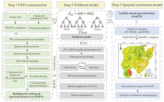
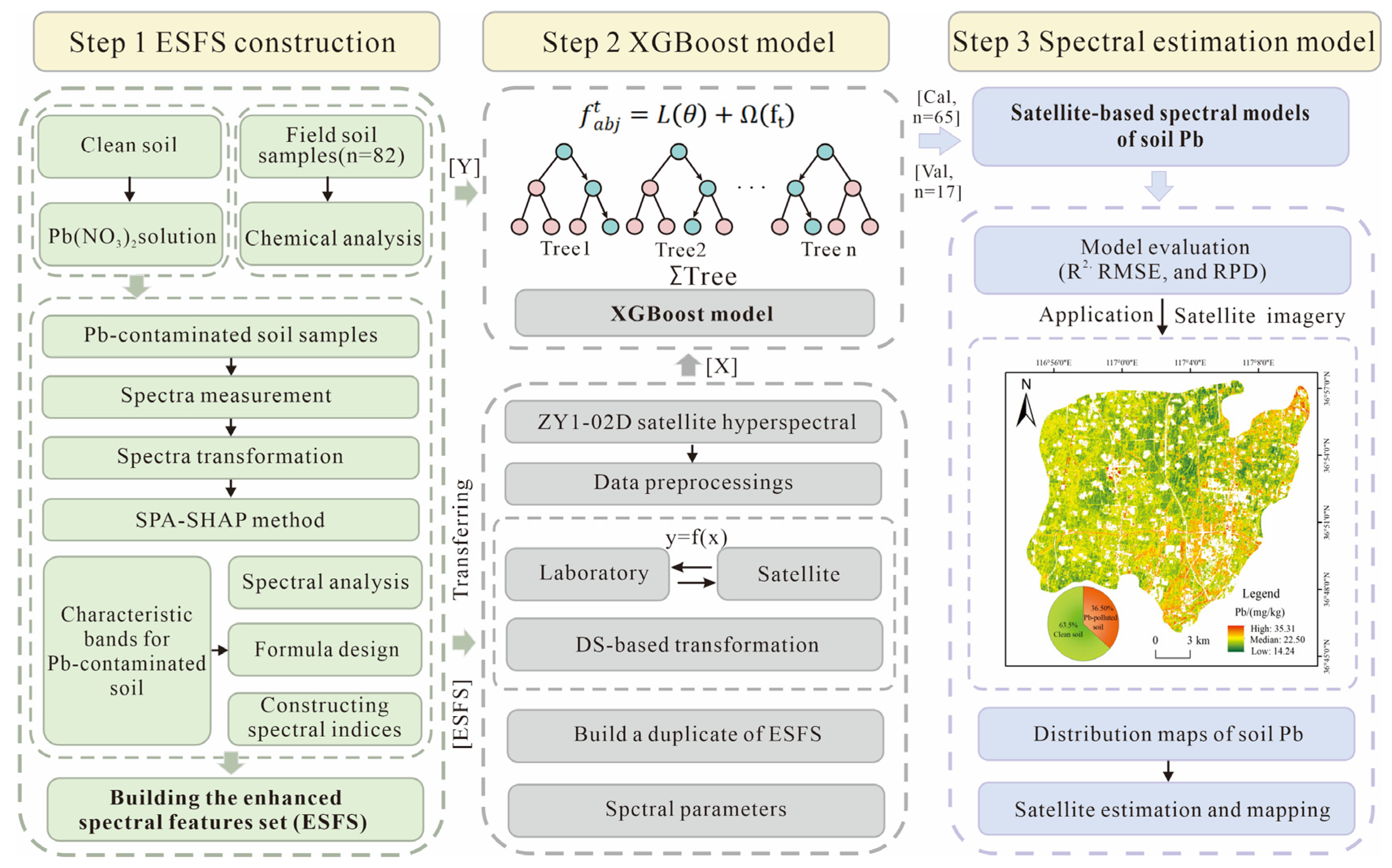
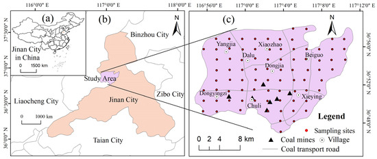
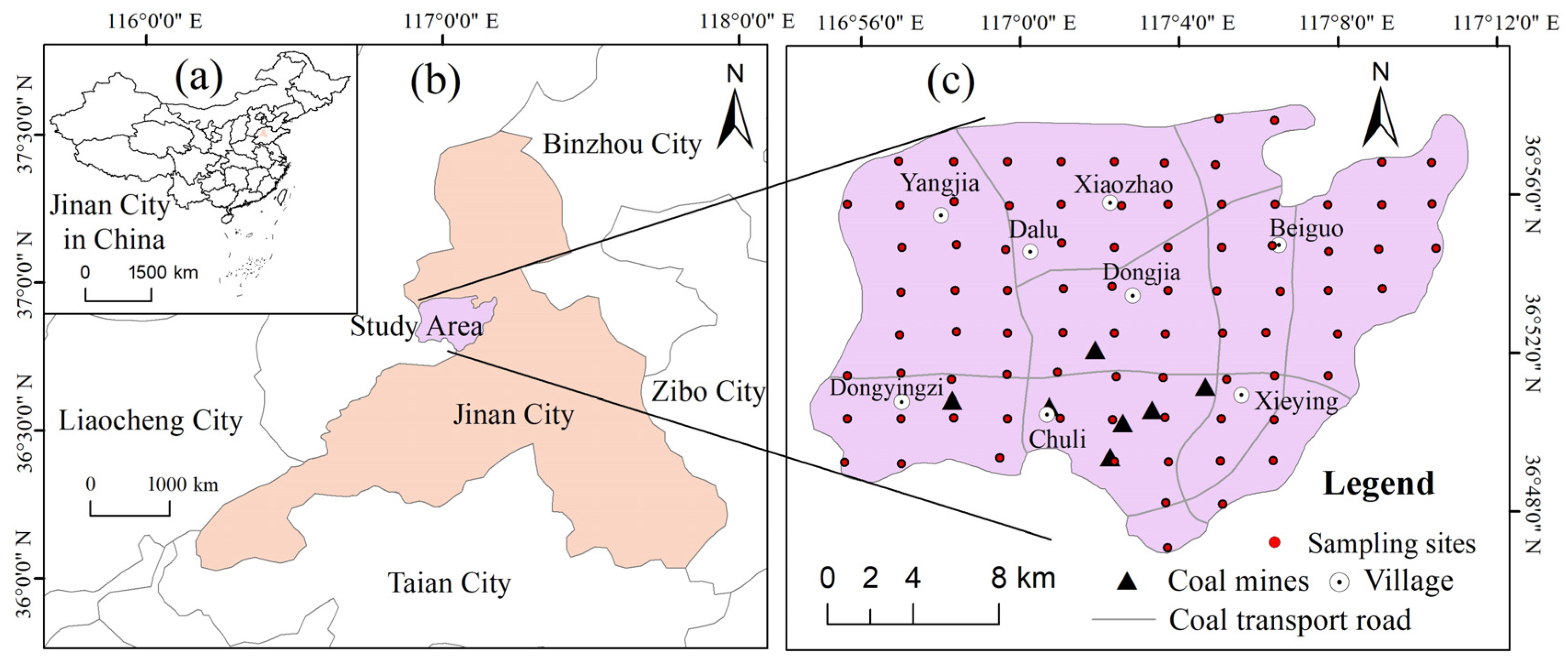
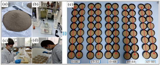
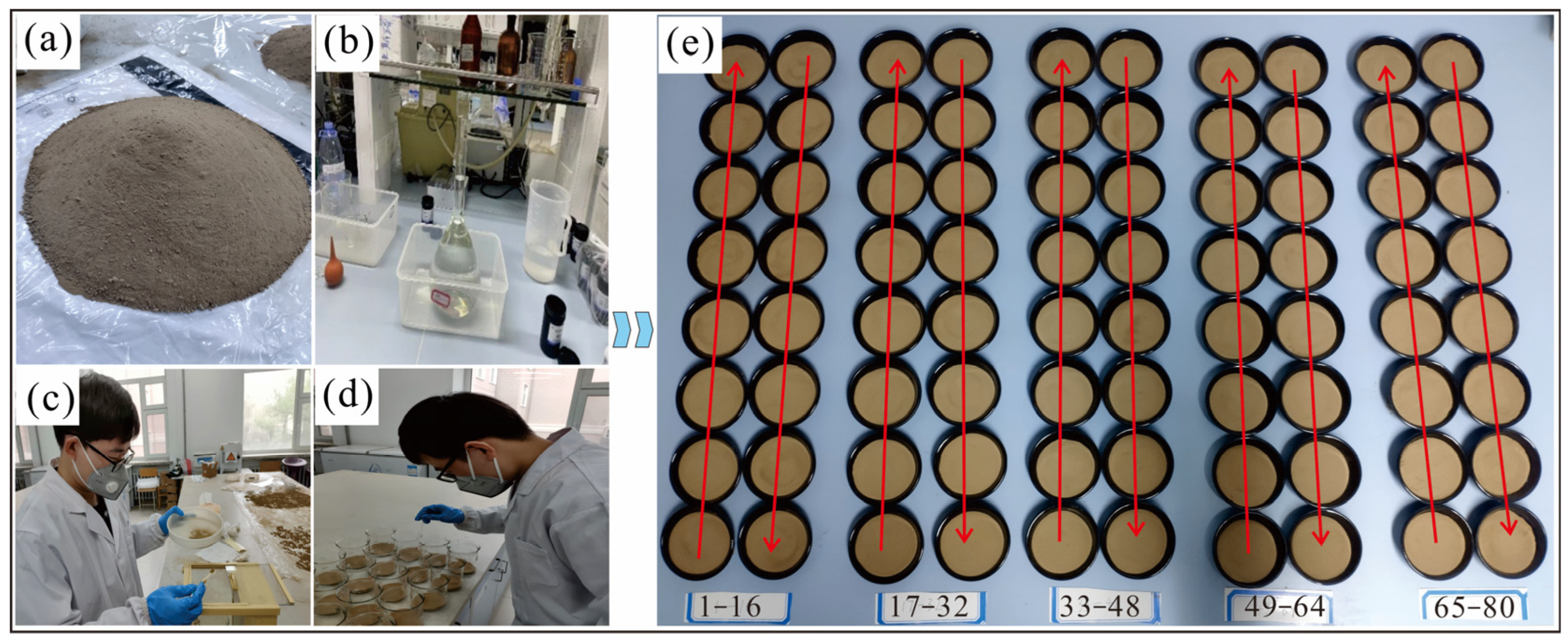
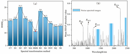
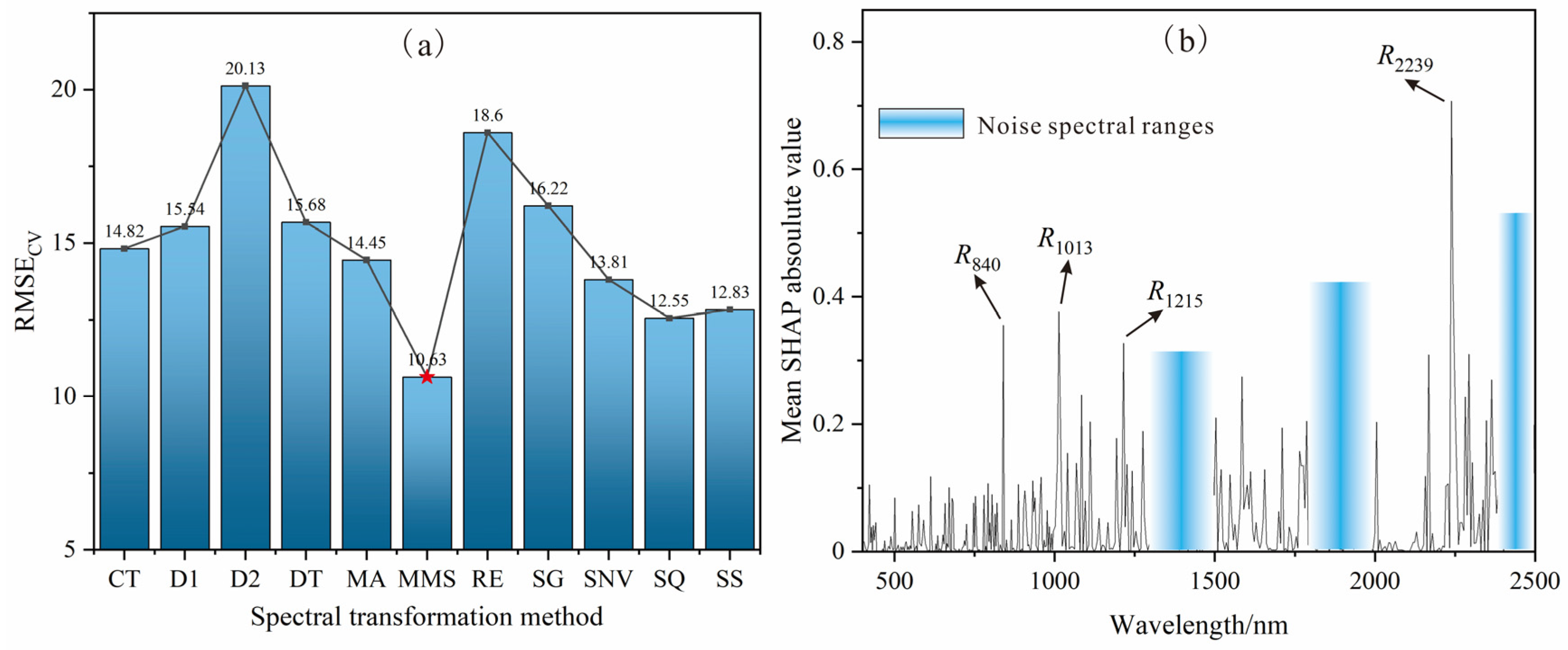
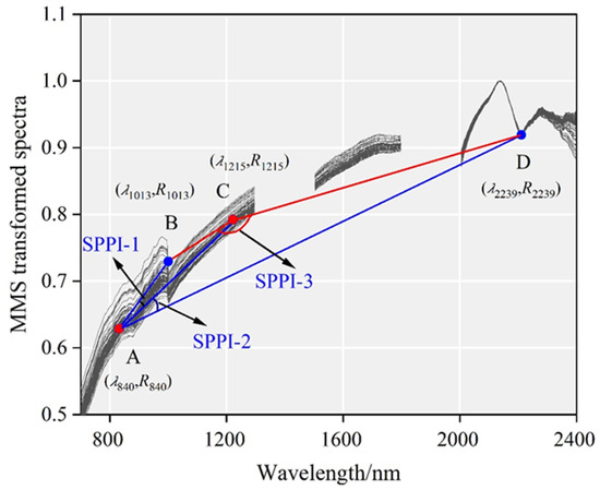
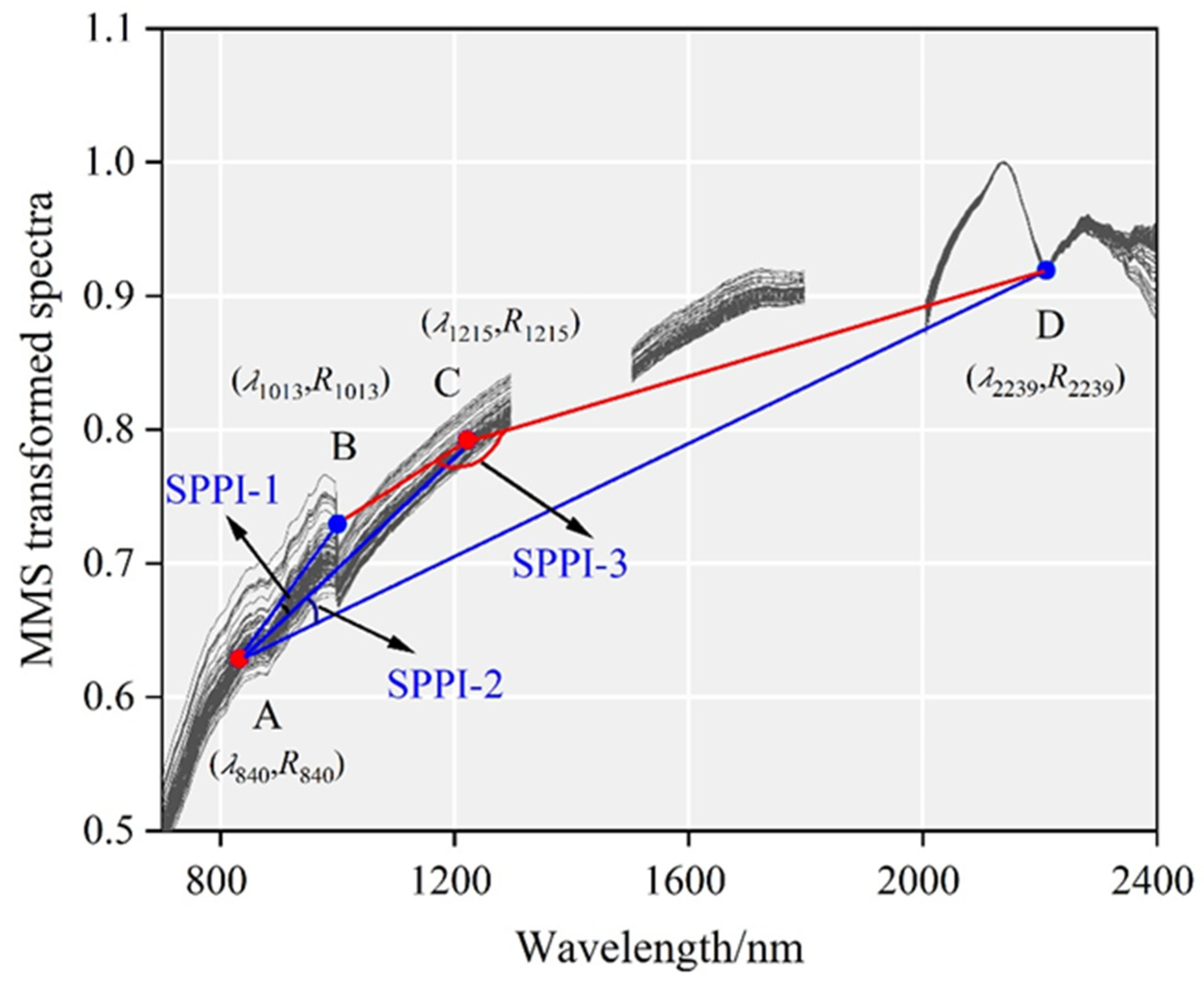
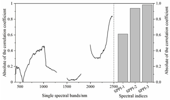
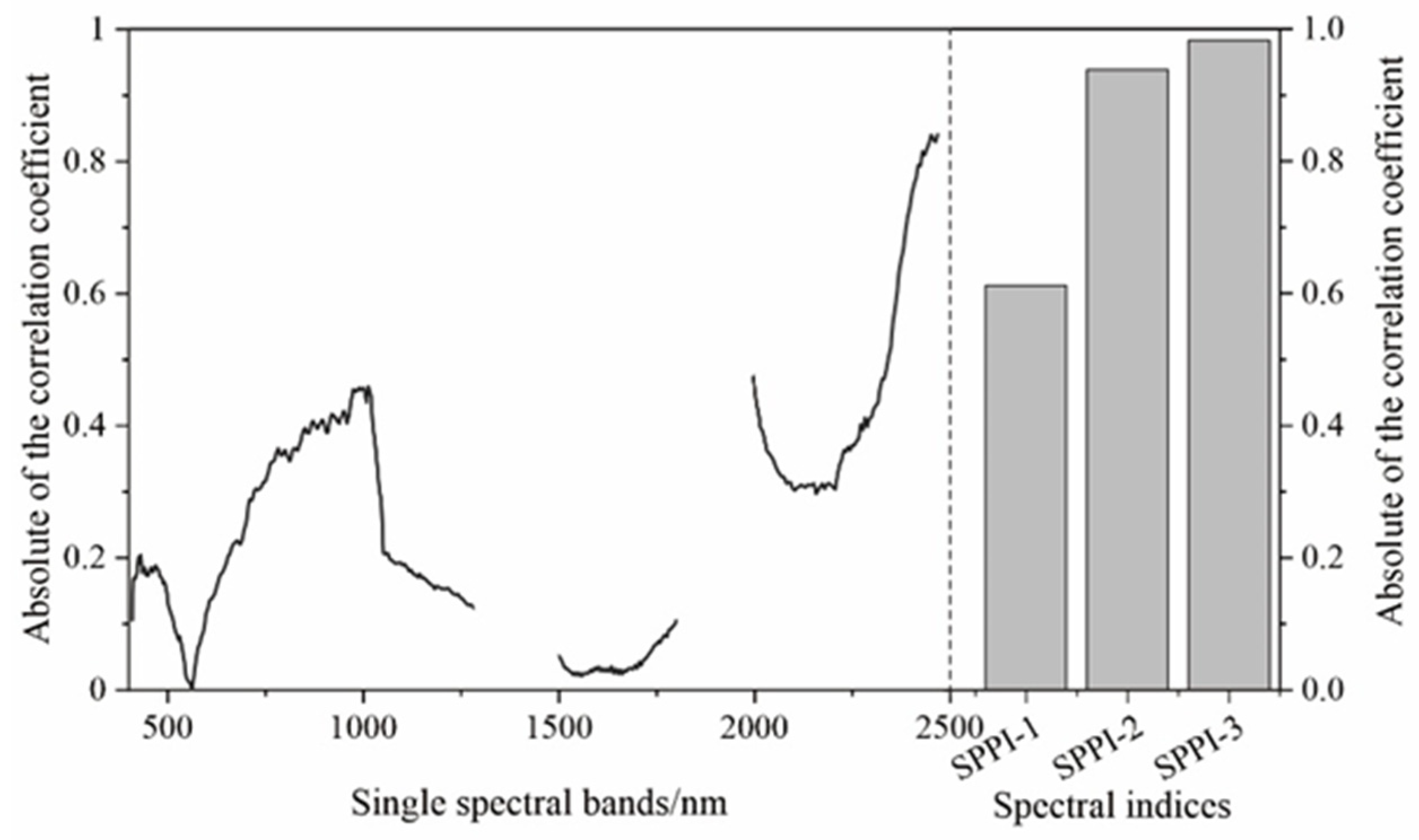
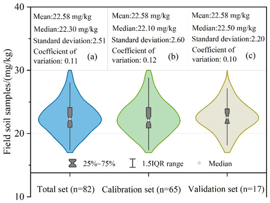
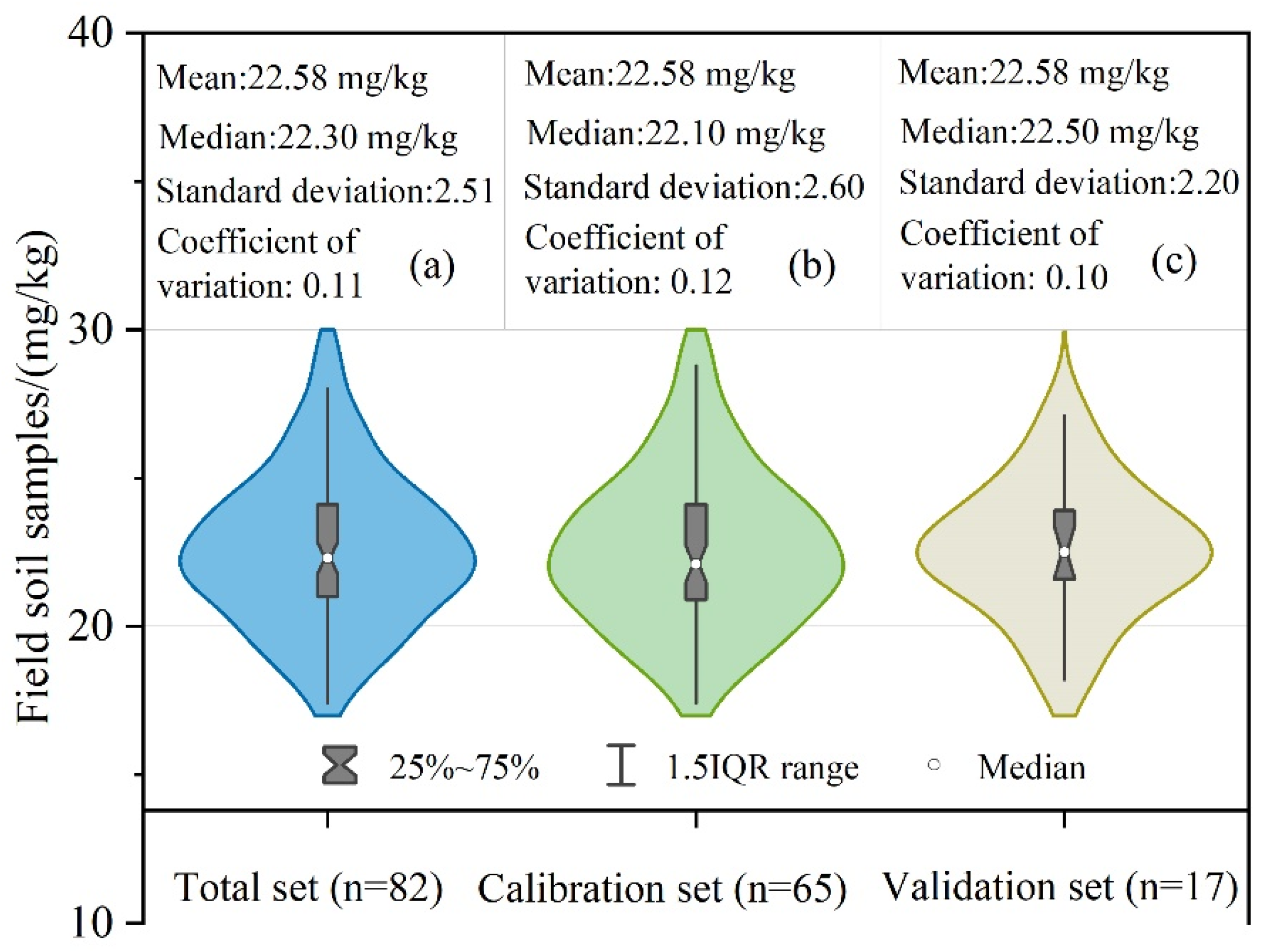
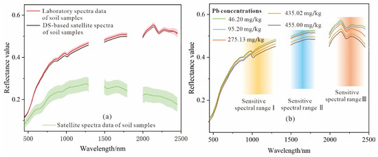
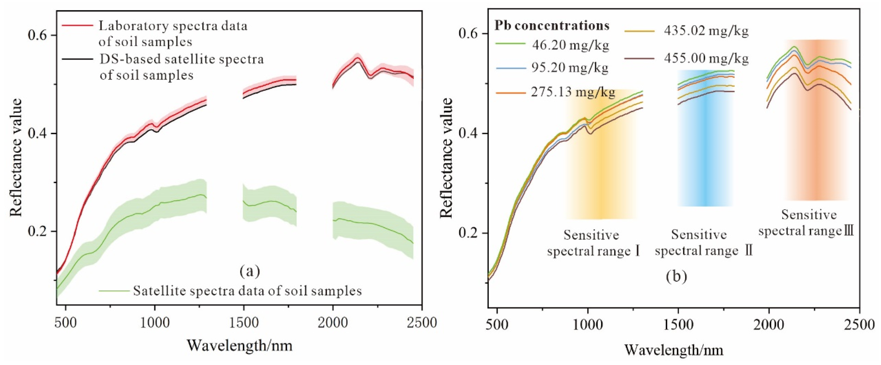
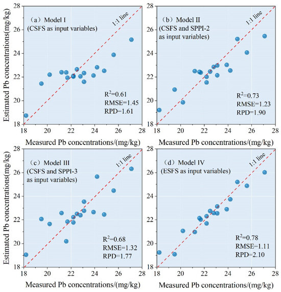
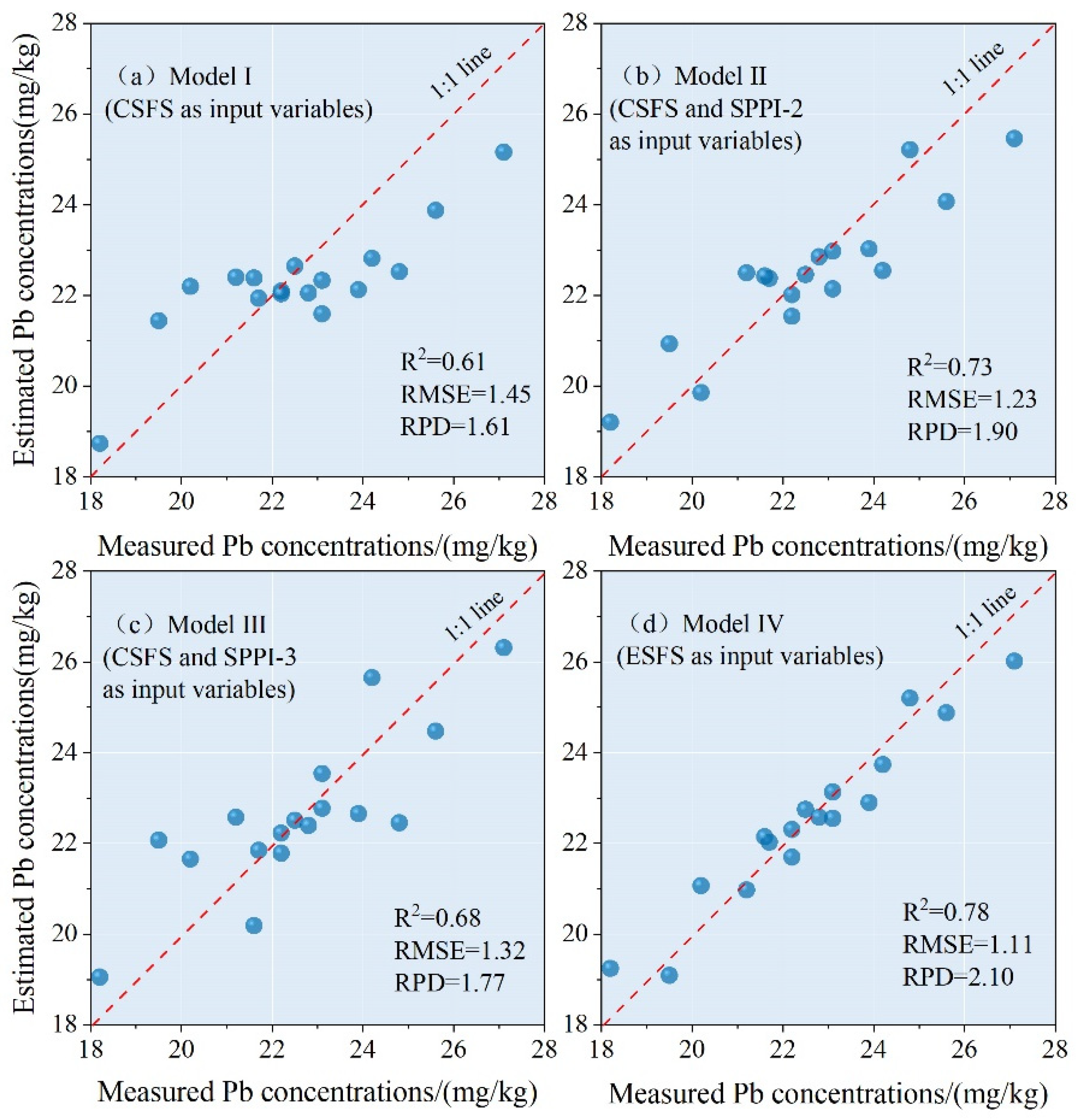
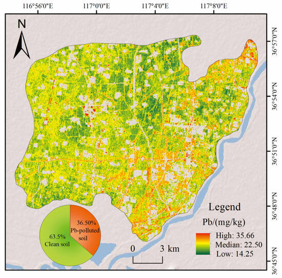
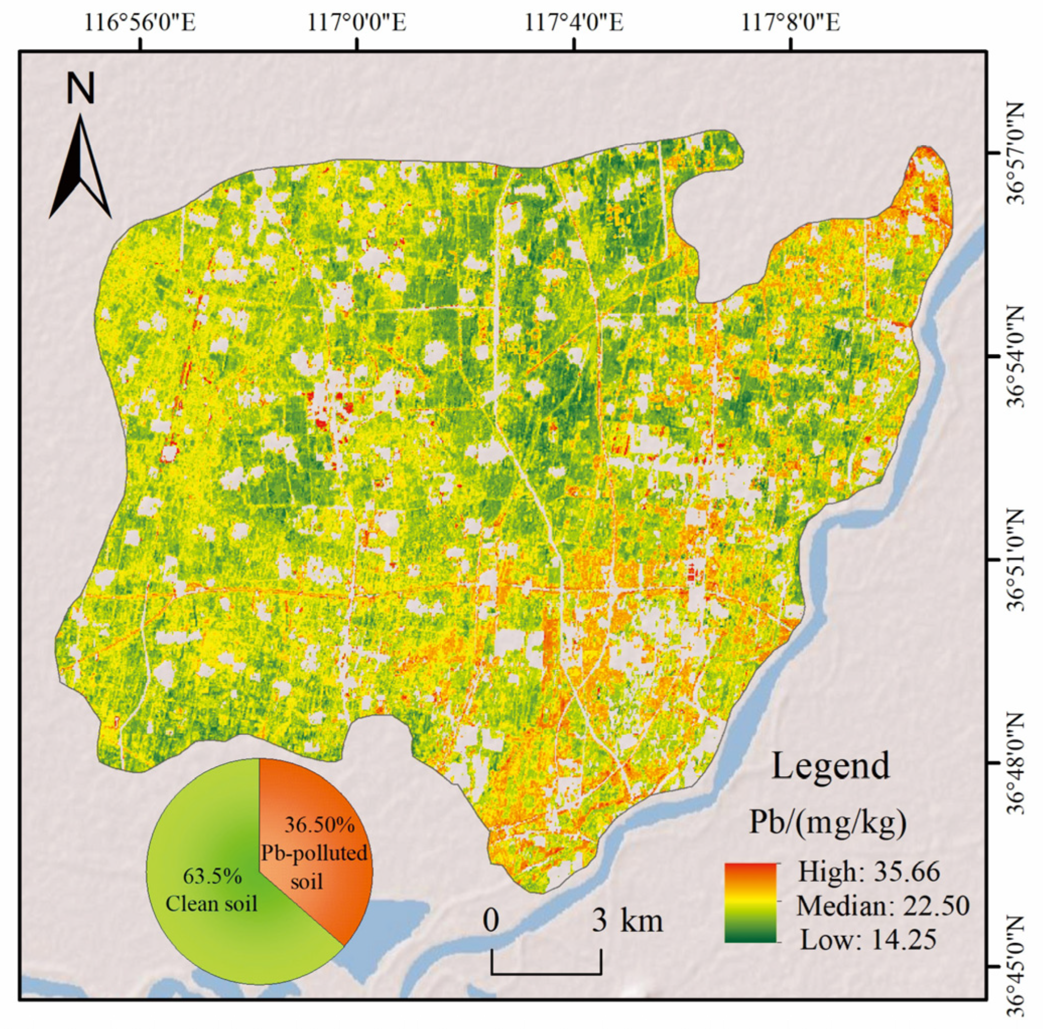
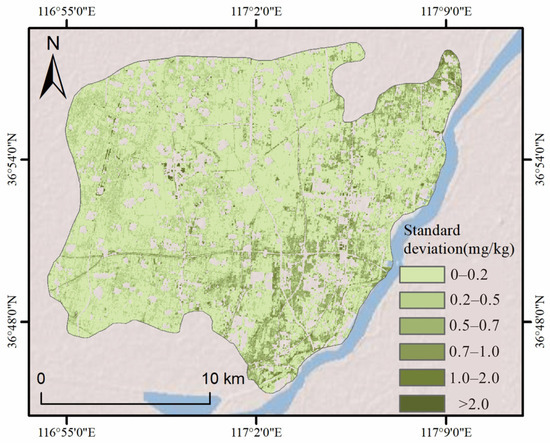
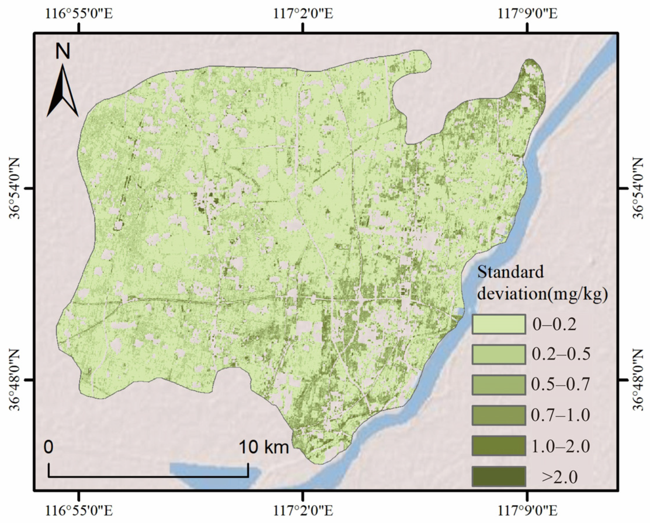
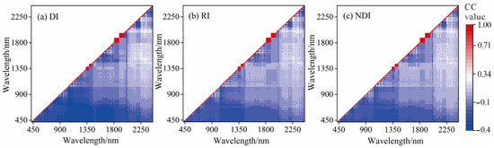
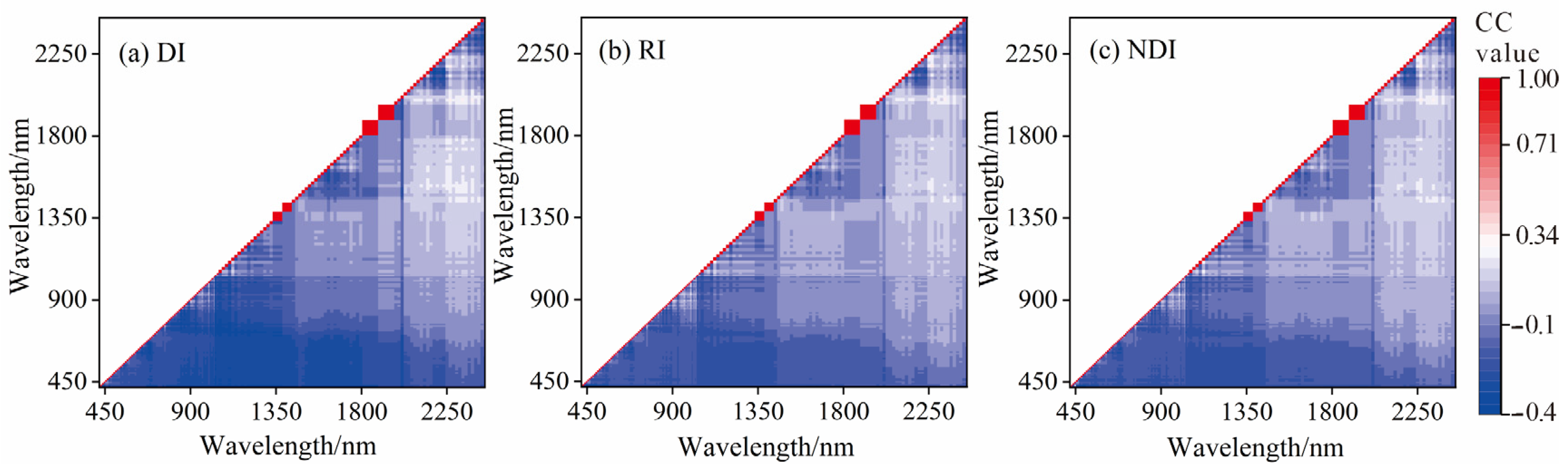

Disclaimer/Publisher’s Note: The statements, opinions and data contained in all publications are solely those of the individual author(s) and contributor(s) and not of MDPI and/or the editor(s). MDPI and/or the editor(s) disclaim responsibility for any injury to people or property resulting from any ideas, methods, instructions or products referred to in the content. |
© 2026 by the authors. Licensee MDPI, Basel, Switzerland. This article is an open access article distributed under the terms and conditions of the Creative Commons Attribution (CC BY) license.