


Highlights
What are the main findings?
- A novel LISA-based framework is proposed to quantify local anthropogenic CO2 increments (dXCO2) within urban agglomerations using a seamless satellite XCO2 dataset.
- Significant spatial heterogeneity in dXCO2 is observed across China’s three major urban agglomerations, with the northern heavy industrial region (BTH: 3.46 ppm) exhibiting much higher values than the southern coastal economic zones (YRD: 1.3 ppm; PRD: 0.08 ppm) during 2015–2019.
- Four dominant modes governing XCO2 anomalies are identified via EOF analysis, revealing multi-scale influences from anthropogenic–natural trade-offs, the East Asian summer monsoon, local emission events, and geographical background.
- Differential responses to COVID-19 lockdowns are captured, with dXCO2 decreasing in BTH and YRD but increasing in PRD, highlighting the modulating role of regional industrial structures.
What are the implications of the main findings?
- The LISA-based method provides a new technical pathway for regionally differentiated emission reduction assessments by enabling the extraction of anthropogenic signals from background variability.
- The observed spatial–temporal patterns and the influence of industrial structures on emission resilience offer crucial insights for designing targeted and effective climate mitigation policies in complex urban agglomerations.
- The successful application of the seamless XCO2 dataset demonstrates its strong potential for monitoring long-term CO2 changes and verifying emission reduction efforts from space.
Abstract
Quantifying anthropogenic CO2 increments is vital for assessing emission reductions. Using a seamless XCO2 dataset over China reconstructed from OCO-2/3 satellite retrievals and machine learning, combined with EOF decomposition and LISA analysis, this study investigates XCO2 anomalies and local anthropogenic increments (dXCO2) at national and urban agglomeration scales. Nationally, XCO2 anomalies exhibit a “southeast positive, northwest negative” spatial pattern aligning with human activities and a “winter high, summer low” seasonal cycle. EOF analysis reveals four dominant modes: anthropogenic–natural trade-offs, East Asian summer monsoon modulation, local emissions, and baseline context. At the regional scale, multi-year mean dXCO2 (2015–2019) in Beijing–Tianjin–Hebei (BTH), Yangtze River Delta (YRD), and Pearl River Delta (PRD) are 3.46 ± 0.45 ppm, 1.30 ± 0.36 ppm, and 0.08 ± 0.14 ppm, respectively, showing higher values in northern heavy industrial zones. During the 2020–2022 pandemic, dXCO2 decreased in BTH (2.28 ± 0.73 ppm) and YRD (1.16 ± 0.43 ppm) but increased in PRD (0.28 ± 0.27 ppm). Compared to pre-pandemic levels, lockdowns saw dXCO2 decrease slightly in YRD while increasing in BTH and PRD, reflecting differential responses of regional industrial structures. This study demonstrates the potential of seamless XCO2 data for monitoring anthropogenic enhancement signals, and the proposed LISA-based method offers new support for regionally differentiated emission reduction assessments.
1. Introduction
Since the Industrial Revolution, global greenhouse gas emissions have surged, and the consequent climate change has been scientifically substantiated [1]. Among these, CO2, as the primary greenhouse gas emitted from fossil fuel combustion, contributes over 60% to total global radiative forcing [2]. Human activities are the main source of CO2 emissions. Cities, as concentrated areas of human activity, host more than half of the global population and the vast majority of economic activities, contributing over 70% of CO2 emissions despite occupying only a small fraction of the Earth’s land surface [3]. The Paris Agreement explicitly sets the goal of limiting global average warming to well below 2 °C and pursuing efforts to limit it to 1.5 °C [4], requiring countries to achieve net-zero emissions by mid-century. To meet this goal, accurately quantifying the increment in atmospheric CO2 concentration caused by human activities, assessing the effectiveness of national emission reduction efforts, and identifying key emission areas have become critical scientific supports for climate governance.
Traditional “bottom-up” observation methods based on ground-based monitoring networks are limited by sparse station distribution, making it difficult to cover emission hotspot areas and resolve the spatial heterogeneity of anthropogenic emissions. The emergence of carbon satellites has provided a new pathway for large-scale, high-precision observation of atmospheric CO2, establishing them as crucial tools for current global carbon cycle research and carbon emission monitoring. For instance, Hakkarainen et al. utilized OCO-2 data to achieve, for the first time, direct spatial observation of localized CO2 emission areas [5]; Schwandner et al. confirmed the capability of spaceborne platforms to detect localized CO2 emission sources [6]. “Top-down” inversion methods based on carbon satellite observation data have become a key technical means for independently assessing and verifying national and regional emission reports.
By differencing observed XCO2 against background concentrations, carbon satellites can effectively identify and quantify XCO2 enhancement signals resulting from both natural processes and human activities. This method has become an important paradigm in current carbon cycle research. Sheng et al., based on OCO-2 data over the Yangtze River Delta urban agglomeration in China, found that XCO2 around major cities and industrial activity intensive areas increased by an average of 1.36~4.41 ppm [7]; Ye et al., focusing on the Xiamen–Zhangzhou–Quanzhou metropolitan area and utilizing high-resolution snapshot data from OCO-3, observed XCO2 enhancements ranging from 0.70 ± 0.53 ppm to 2.29 ± 1.16 ppm, and further constrained anthropogenic CO2 emissions in the Xiamen area using Bayesian inversion methods [8]; Ji et al., by analyzing 473 global OCO-2 observation cases from 2014 to 2023, successfully retrieved point-source scale CO2 emissions, finding a global average emission rate of 6166.52 t CO2/h, with case studies in California, Riyadh, and Xinjiang further validating the effectiveness of satellite differencing methods in capturing localized emission plumes [9]. At the urban scale, Xu et al. utilized OCO-3 XCO2 observations combined with Gaofen-5 and TROPOMI NO2 data to identify enhancements from 69 global emission sources, showing that anthropogenic emission signals in regions such as East Asia, Europe, the Middle East, and North America were effectively captured, with approximately 45% of estimated emissions lower than inventory reports, reflecting the potential of satellite observations for independent verification [10]. These studies indicate that by differencing satellite-observed XCO2 from appropriate background values, the resulting increments can effectively reflect contributions from different sources, providing a key technical means for distinguishing between natural and anthropogenic signals.
However, constrained by satellite observation conditions and scanning modes, most existing studies have been limited to point-source scales [11]. Consequently, effectively identifying anthropogenic enhancement signals at the urban agglomeration scale from continuous XCO2 fields remains a pressing challenge. To address this issue, this study leverages a high-resolution, spatially and temporally continuous XCO2 dataset over China—constructed from OCO-2 and OCO-3 satellite retrievals—to systematically investigate the spatiotemporal evolution of XCO2 increments induced by human activities at both national and intra-urban agglomeration scales. Specifically, spatial overlay analysis is first employed to examine the spatial correspondence between areas of elevated XCO2 concentrations and high carbon emission intensities, thereby assessing the capability of the concentration field to indicate ground-level emission sources across different regions. Subsequently, empirical orthogonal function (EOF) decomposition is applied to extract the dominant spatiotemporal structures of the XCO2 anomaly field and to identify the principal modes of variability and their temporal evolution. Building upon this foundation, a technical framework integrating high-resolution XCO2 spatial distributions with spatial autocorrelation analysis is proposed, with a focus on three major urban agglomerations—the Beijing–Tianjin–Hebei region, the Yangtze River Delta, and the Pearl River Delta. This framework aims to isolate local anthropogenic CO2 increments within urban agglomerations and to characterize their spatial heterogeneity, thereby providing a scientific basis for the formulation of regionally differentiated emission reduction policies.
2. Materials and Methods
2.1. Data
2.1.1. XCO2 Dataset
The TAF-XCO2 (Temporally Adaptive Forest) [12] dataset employed in this study spans the China region from January 2015 to December 2022, with a spatial resolution of 0.01° × 0.01° and a monthly temporal resolution. This dataset is a seamless reconstruction product generated using the Temporally Adaptive Forest method based on XCO2 retrievals acquired by the OCO-2 satellite [13,14] (January 2015–December 2022) and the OCO-3 satellite [15] (September 2019–December 2022); comprehensive methodological details have been documented in a dedicated data descriptor publication. Specifically, the OCO-2 XCO2 retrievals were obtained from the OCO2_L2_Lite_FP product (v11.1r), and the OCO-3 XCO2 retrievals from the OCO3_L2_Lite_LP product (v10.4r), both of which were provided by the Goddard Earth Sciences Data and Information Services Center (GES DISC, https://disc.gsfc.nasa.gov/). Previous investigations have indicated that the XCO2 estimates from the two satellites differ by approximately 0.2 ppm over land and 0.3 ppm over ocean [16]. Despite the non-overlapping observational periods of the two satellites, their data were jointly utilized in this study to enhance the completeness and continuity of spatiotemporal coverage.
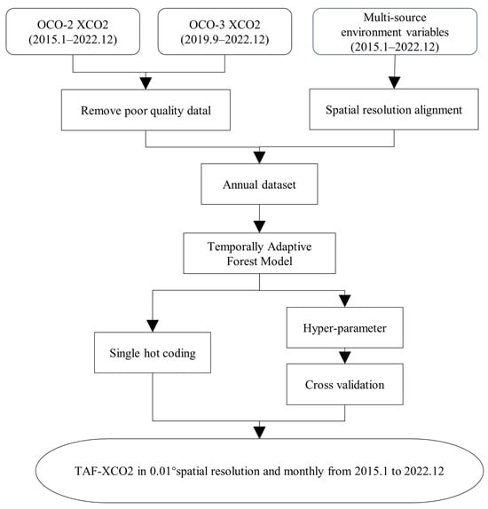
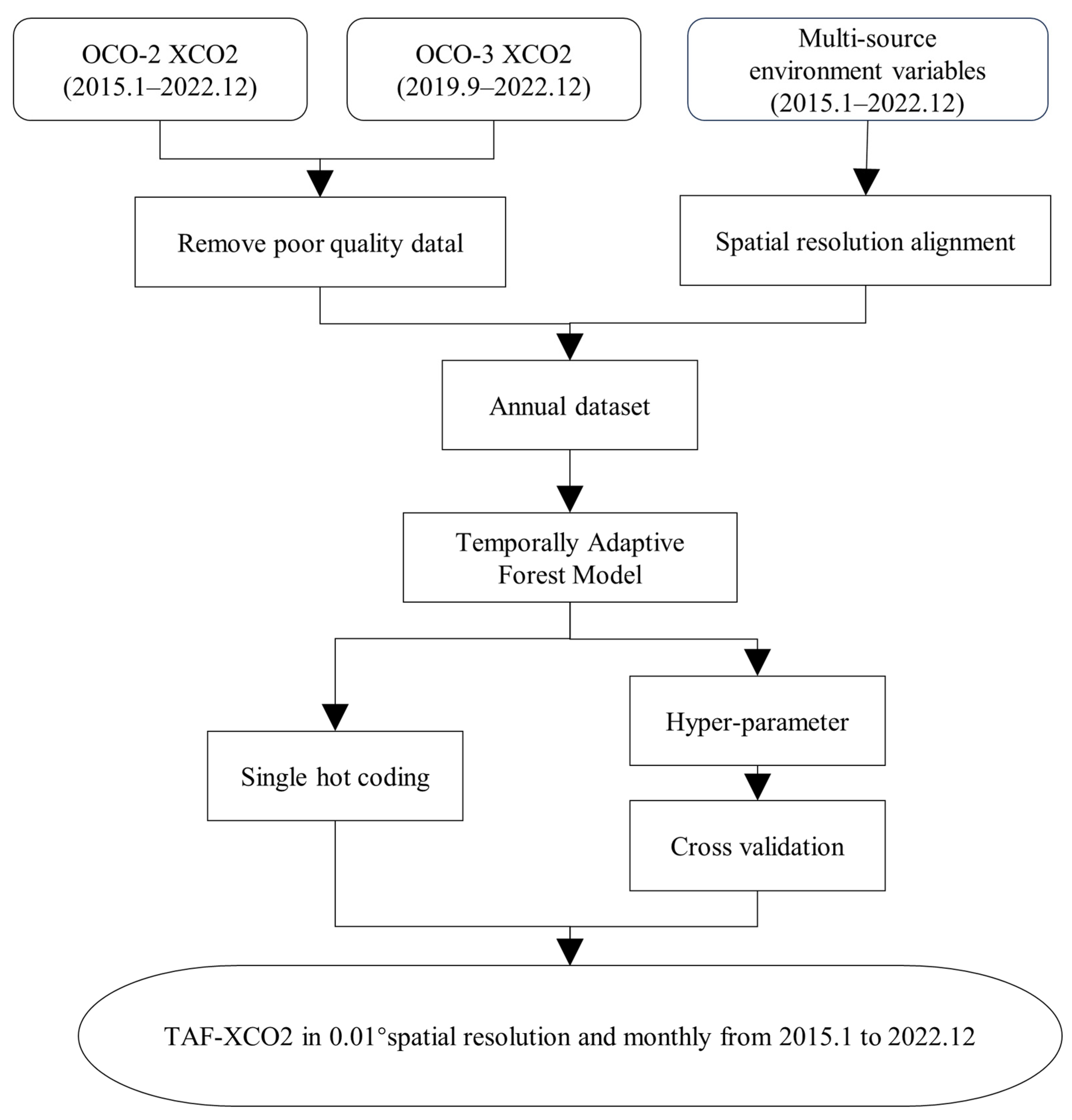
The TAF-XCO2 dataset was constructed based on the Temporally Adaptive Forest (TAF) model [12]. The overall workflow is illustrated in Figure 1. First, a unified input layer was established by resampling all environmental variables to an identical spatial resolution and coordinate system. Subsequently, feature-layer optimization was performed: for categorical variables, an annually dynamic one-hot encoding strategy was adopted to ensure optimal alignment between feature representation and the data distribution of the corresponding year; for continuous variables, standardization was applied to eliminate the influence of disparate dimensional units. On this basis, a grid search coupled with three-fold cross-validation was employed to optimize the model hyperparameters on an annual basis, including the number of decision trees, maximum tree depth, and the minimum number of samples required at a leaf node. The training dataset was randomly partitioned into three subsets, with two subsets serving as the training set and the remaining subset as the validation set. The optimal hyperparameter combination for each year was determined by minimizing the root mean square error (RMSE). The annually optimized hyperparameter results are presented in Table A1. Using the optimized hyperparameters, independent regression models were constructed for each year and trained on the respective annual training sets to learn the complex nonlinear mapping relationships between multi-source environmental variables, including vegetation indices (e.g., NDVI, EVI, GPP), meteorological elements (Temperature, Precipitation, Wind speed, Potential evapotranspiration, and Surface pressure), emission-related variables (Fossil fuel emission, NO2), and topographic factors (digital elevation model), and XCO2. After model training, the independent variable data for all twelve months of a given year were fed monthly into the corresponding annual TAF model to generate monthly XCO2 prediction raster images. Ultimately, through the sequential output of independently trained annual models, a monthly seamless XCO2 dataset for China at a spatial resolution of 0.01° was produced for the period 2015–2022.
Figure 1.
Workflow for reconstructing XCO2 distribution using satellite XCO2 retrieval data.
Independent validation against ground-based station observations demonstrates that the TAF-XCO2 data exhibit strong consistency with TCCON measurements: at the Hefei station, the R2 value reaches 0.89 with an RMSE of 1.387 ppm, while at the Xianghe station, the R2 is 0.737 with an RMSE of 2.026 ppm.
The CAMS XCO2 data (Copernicus Atmosphere Monitoring Service) is a global gridded atmospheric CO2 column concentration reanalysis product generated by assimilating multi-source satellite and ground-based observations combined with atmospheric transport models. It offers advantages such as spatiotemporal continuity and scientific reliability, providing crucial data support for carbon cycle research, satellite validation, and emission estimation. In this study, monthly composites of CAMS XCO2 data are used for comparative analysis of spatiotemporal variability with TAF XCO2. This dataset has a spatial resolution of 0.75° × 0.75°, covering the period from January 2015 to December 2020, and is sourced from the European Centre for Medium-Range Weather Forecasts (https://ads.atmosphere.copernicus.eu/, accessed on 28 April 2026).
All datasets utilized in this study are summarized in Table 1.
Table 1.
Data Sources Used for XCO2 Reconstruction.
2.1.2. Carbon Emission Data
EDGAR (Emission Database for Global Atmospheric Research) is an authoritative global anthropogenic greenhouse gas emissions dataset developed and maintained by the Joint Research Centre (JRC) of the European Commission [17]. This database (https://aqmx.org) provides long time-series emission data from 1970 to the present. Its latest version integrates collaborative results from the JRC and the International Energy Agency (IEA) [18], covering a full range of major greenhouse gases including carbon dioxide (CO2), methane (CH4), nitrous oxide (N2O), and fluorinated gases, with a spatial resolution of 0.1° × 0.1°. This study utilizes the annual carbon emission data from this dataset for the period 2015–2022.
2.2. Methods
To systematically resolve the spatial structure of XCO2 anomalies, this study employs three complementary analytical methods in sequence. First, spatial overlay analysis is conducted to evaluate the spatial consistency between concentration hotspots and emission sources, thereby clarifying the applicable premise of anthropogenic increment detection. Next, empirical orthogonal function (EOF) analysis is applied to isolate the dominant modes of variability across different scales. Finally, the local indicator of spatial association (LISA) is utilized to extract localized increment signals attributable to anthropogenic emissions.
2.2.1. Spatial Overlay Analysis
This study aims to effectively extract the local enhancement signals attributable to anthropogenic emissions from the continuously distributed XCO2 concentration field. It should be noted that satellite-observed XCO2 column concentrations inherently result from the combined effects of surface emissions, atmospheric transport processes, and natural sources and sinks. Consequently, in the absence of fundamental spatial consistency between regions of elevated XCO2 concentrations and hot pixels of anthropogenic carbon emissions, subsequent analyses that seek to identify anthropogenic enhancement based on the concentration field would lack the requisite prerequisite foundation. To quantitatively assess the degree of spatial correspondence between the two, this study employs a spatial overlay analysis method. Specifically, this approach calculates the proportion of the overlapping area between pixels with high XCO2 concentrations and those with high carbon emissions relative to the total area of high-emission pixels, thereby establishing a quantitative metric that characterizes the spatial consistency between emissions and observed concentrations. The calculation formula is as follows:
The (OR) effectively identifies areas potentially influenced by anthropogenic emissions contributing to the increase in regional atmospheric CO2 concentration.
2.2.2. Empirical Orthogonal Function Analysis
The spatiotemporal variability of XCO2 is subject to the compounded influences of monsoonal transport, vegetation phenology, interannual climate oscillations, and anthropogenic emission fluctuations. Analyzing these individual processes is therefore essential to mitigate the background interference imposed by natural variability. To this end, the empirical orthogonal function (EOF) method is introduced. Empirical Orthogonal Function analysis is a statistical method for parsing the spatiotemporal variability of large, multi-dimensional datasets and is widely applied in various geographical fields such as atmospheric science and oceanography [19,20,21]. As a form of principal component analysis, the EOF method decomposes multi-dimensional data into a set of orthogonal spatial patterns (EOFs) and their corresponding temporal coefficients (PCs), ordered by their variance contribution. This ensures that the leading modes explain the majority of the variance in the original dataset [22].
Let the original data matrix be . First, its spatial covariance matrix is calculated:
where denotes the covariance matrix, the subscript indicates the spatial domain, the superscript denotes matrix transpose, and is the number of spatial samples. Eigendecomposition is performed on the covariance matrix:
Here, is the eigenvector matrix, whose column vectors correspond to the temporal coefficients (PCs); is a diagonal matrix whose diagonal elements are the eigenvalues. Since the dimension of the covariance matrix equals the number of observations, each eigenvector represents a time series.
Projecting the spatial anomaly matrix onto the eigenvector matrix yields the corresponding spatial modes (EOFs):
where each column of represents a spatial mode. The original data can be reconstructed from the spatial modes and temporal coefficients:
The variance contribution rate of each EOF/PC mode is obtained by dividing its corresponding eigenvalue by the sum of all eigenvalues. Modes are ordered by the amount of variance they explain; the first mode explains the largest fraction of variance, the second mode explains the next largest, and so on. This ordering property enables the EOF method to effectively extract dominant spatiotemporal variability signals, rendering it well-suited for identifying the principal modes of variation in complex regions and thereby providing a crucial characterization of the background field for the subsequent incremental separation focused on the urban agglomeration scale.
2.2.3. Identifying Local Anthropogenic Emission Increments Based on LISA
Spatial autocorrelation is a statistical metric for measuring spatial dependence, which can be categorized into global autocorrelation and local autocorrelation based on spatial scale [23]. To identify the degree of autocorrelation between each spatial unit and its neighboring units, and to quantitatively characterize the spatial association differences across various regions, this study employs the Local Moran’s I (LISA) method [24,25]. For a spatial location , the calculation formula for LISA is:
where andare the standardized deviations of the observed values from the mean for spatial units and , respectively; denotes the total number of pixels; is the spatial weight matrix, which is row-standardized during model computation.
The test statistic for the significance of LISA is the score, calculated as follows:
where is the LISA value, is its expected value, and is its variance.
Under the condition that the score is significant, the LISA result can be interpreted as four types of spatial association [26]: ① When > 0 and > 0, it indicates that unit and its neighbors are both high values, representing a High–High cluster (HH); ② When > 0 and < 0, it indicates that unit and its neighbors are both low values, representing a Low–Low cluster (LL); ③ When < 0 and > 0, it indicates that unit is a high value while its neighbors are low values, representing a High–Low outlier (HL); ④ When < 0 and < 0, it indicates that unit is a low value while its neighbors are high values, representing a Low–High outlier (LH).
Ideally, CO2 concentrations should be elevated in proximity to emission sources and decline with increasing distance, exhibiting a spatial distribution consistent with Tobler’s First Law of Geography. Traditional background subtraction methods typically rely on the mean concentration within a single latitudinal band as the background value. This approach introduces substantial biases in regions characterized by dense emission sources interspersed with surrounding natural carbon sinks. To overcome this limitation, the present study applies LISA to the analysis of XCO2 data in order to identify spatial clustering patterns of elevated XCO2 values. A significance threshold of p ≤ 0.05 was adopted for cluster classification. By objectively delineating the spatial extent of emission hotspots directly from the continuous field, and by accounting for underlying surface heterogeneity, the LISA approach enables a more robust isolation of the net contribution of local anthropogenic emissions to XCO2 concentrations [7]. Since the reconstructed data is in GeoTIFF format, it needs to be converted to point features before analysis to calculate the Local Moran’s I index. Based on this, HH clusters are considered as local anthropogenic emission source areas, and the mean XCO2 value within LL clusters is taken as the background concentration. The background value is extracted using a latitudinal zonal statistics method: first, the mean is calculated for LL points within each 0.01° latitude interval, and then a polynomial fit is applied to construct a background concentration curve across continuous latitudinal bands. The calculation formula for the local anthropogenic CO2 increment () is:
3. Results
3.1. Spatiotemporal Characteristics of XCO2 Across China
The grid-level differences between the reconstructed CO2 concentrations and the national background value represent the combined deviations of ecological fluxes, transport fluxes, and anthropogenic emissions within each grid cell relative to the national average, thereby reflecting the spatial characteristics of carbon sources and sinks [27]. Based on the seamless TAF-XCO2 dataset, gridded XCO2 anomalies (ΔXCO2) over China were derived by subtracting the annual mean national background value from each grid cell, enabling an analysis of the overall distribution patterns and temporal variations of carbon sources and sinks across the country. Concurrently, the CAMS-XCO2 reanalysis product for the same period was incorporated as a comparative validation dataset to further assess the consistency of the results.
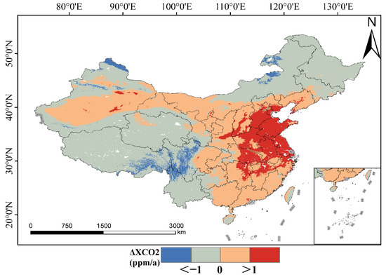
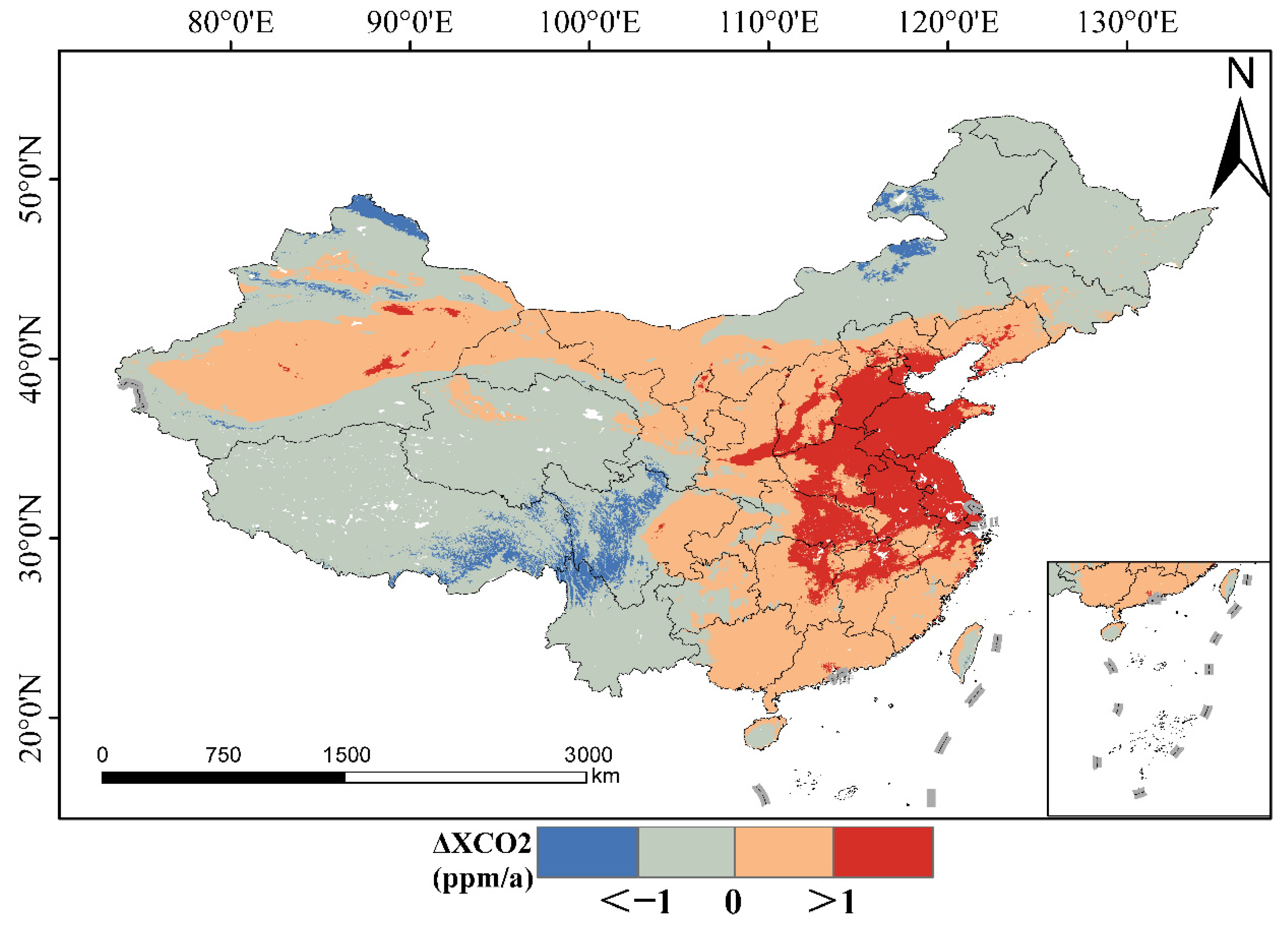
Based on two satellite retrieval datasets, TAF-XCO2 and CAMS-XCO2, this study calculated gridded XCO2 anomalies (ΔXCO2) across China from 2015 to 2020, aiming to reveal the spatiotemporal variation characteristics of carbon sources and sinks in the China region. Figure 2 shows the multi-year average spatial distribution pattern of TAF ΔXCO2, and Figure A1 presents that of CAMS ΔXCO2. The two data products exhibit good consistency: significant positive anomalies are observed in the Beijing–Tianjin–Hebei region, the Yangtze River Delta, and Central China, whereas negative anomalies are found in Northeast and Southwest China. However, numerically, TAF-XCO2 is approximately 0.53 ppm lower than CAMS-XCO2 in the Beijing–Tianjin–Hebei region but significantly higher in most parts of the western region. Spatially, significant discrepancies are predominantly concentrated in western regions such as Xinjiang and Tibet. These differences likely stem from fundamental distinctions in the underlying data sources, data assimilation schemes, and reconstruction frameworks employed by the two products. Furthermore, the coarser spatial resolution of CAMS XCO2 may effectively smooth out localized variability, whereas the TAF-XCO2 dataset exhibits markedly higher sensitivity to fine-scale regional heterogeneity.
Figure 2.
Spatial distribution of average atmospheric ΔXCO2 in China from 2015 to 2020.
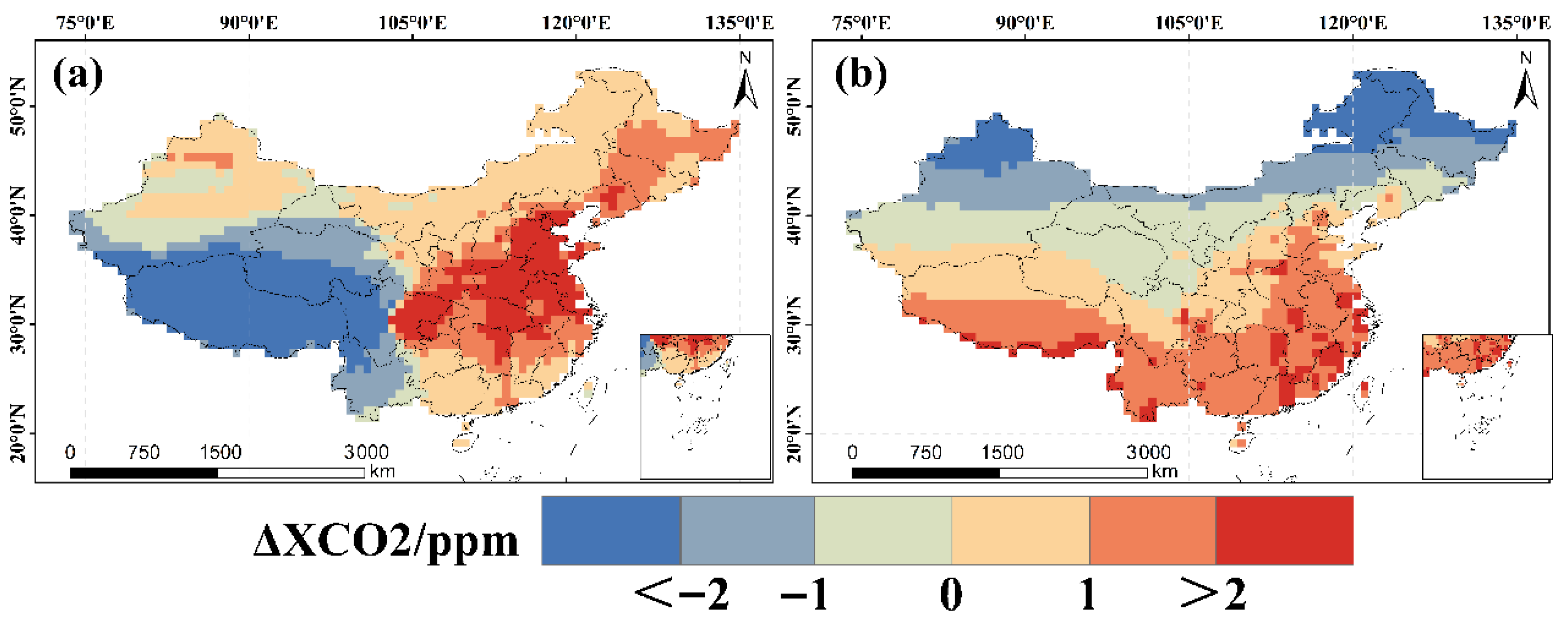
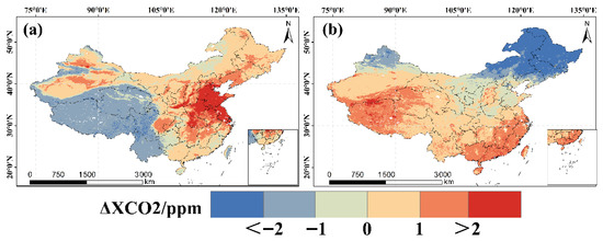
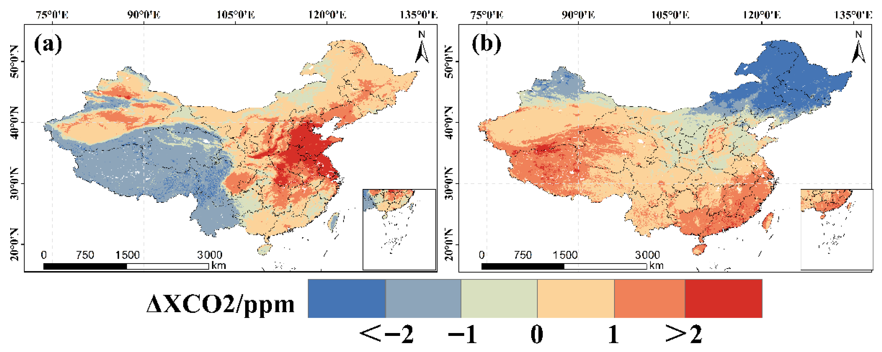
The seasonal ΔXCO2 values for winter and summer were calculated by averaging the ΔXCO2 data over the periods of December–January–February (DJF) and June–July–August (JJA), respectively [28]. On a seasonal scale, Figure 3 illustrates the seasonal spatial patterns of ΔXCO2 retrieved from TAF XCO2 between 2015 and 2020, and Figure A2 shows those from CAMS XCO2. In winter, due to weakened vegetation photosynthesis in the Beijing–Tianjin–Hebei region and Central China, the ecosystem’s CO2 absorption capacity reaches its minimum. The spatial distribution of ΔXCO2 is primarily dominated by fossil fuel emissions from heating activities [29]. Shandong Province, western Hebei Province, and Henan Province exhibit pronounced positive anomaly areas, with ΔXCO2 exceeding 2 ppm. Between 32°N and 50°N, ΔXCO2 is generally positive, while in summer it turns negative, with some areas below −1 ppm, further confirming the seasonal contribution of winter heating emissions. In summer, the strongest negative ΔXCO2 anomalies appear in the relatively high-latitude areas of China. These regions, characterized by lower intensity of human activities coupled with vigorous vegetation regrowth leading to stronger CO2 uptake, result in significantly negative ΔXCO2 [30]. Overall, ΔXCO2 in the China region exhibits a general pattern of “higher values in winter and lower values in summer” [31], with the exception of the Southwest region, which shows negative anomalies in winter and positive anomalies in summer. The seasonal distribution patterns described above are largely consistent with those derived from CAMS-XCO2. It is worth noting that CAMS-XCO2 ΔXCO2 values in summer are generally higher in areas east of the Heihe–Tengchong Line, and its decreasing trend with latitude is smoother, which may be related to smoothing effects resulting from its coarser spatial resolution [32].
Figure 3.
Spatial distribution of seasonal ΔXCO2 from 2015 to 2022: (a) Winter (b) Summer.
To quantitatively assess the spatial coupling characteristics and interannual evolution between regions of high anthropogenic carbon emission activity and areas of elevated atmospheric CO2 concentration over China, this study utilized the EDGAR carbon emission dataset and the TAF-XCO2 product. Grid cells ranking in the top 20% for both emission intensity and XCO2 concentration were designated as emission hot pixels and concentration hot pixels, respectively. This classification was implemented within ArcGIS 10.8 by applying quantile-based symbology to extract the uppermost 20% of grid cells, followed by a spatial overlay analysis. To facilitate this analysis, the TAF-XCO2 data were resampled to match the spatial resolution of the EDGAR dataset. As presented in Table 2, the spatial overlap between the two hot pixels categories ranges from 55.49% to 69.09%, indicating that areas of high CO2 concentration statistically encompass approximately two-thirds of the major ground-level emission sources in most years, thereby demonstrating a reasonable capacity for macroscopic source identification.
Table 2.
Spatial overlap between EDGAR carbon emission hot pixels and CO2 concentration hot pixels in China from 2015 to 2022.
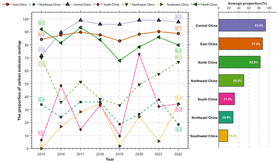
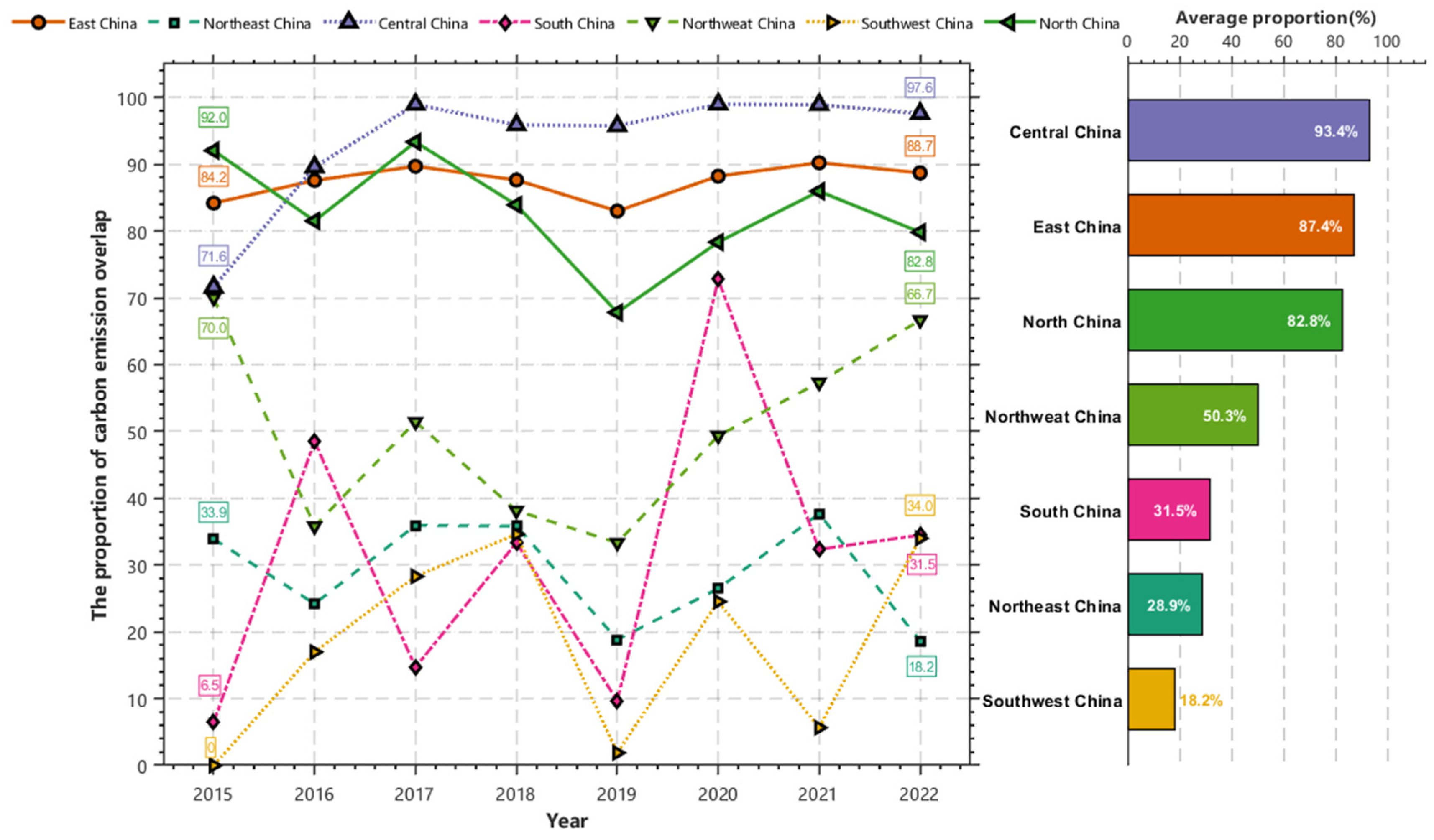
At the regional scale, the “emission–concentration” relationship exhibits significant spatial heterogeneity, leading to considerable differences in the applicability of methods for identifying emission sources based on CO2 concentration hotspots across different regions [33,34]. As shown in Figure 4, Central China, East China, and North China demonstrate a high degree of “emission–concentration” coupling, with overlap ratios exceeding 80%. Here, concentration signals can effectively reflect the pattern of ground-level emissions. In contrast, the overlap ratios in Southwest China, Northeast China, and South China are less than 30%, where CO2 concentration hotspots struggle to reliably capture emission sources. This may be related to factors such as more dispersed emission source distributions, favorable diffusion conditions, or stronger regional carbon sink effects [35]. Northwest China represents a moderate coupling area, with an overlap ratio of approximately 50%, but exhibits substantial interannual variability, reflecting the complexity of the emission–concentration relationship in this region.
Figure 4.
Proportion of carbon emission overlap by region in China from 2015 to 2022.
It is noteworthy that in 2019, the overlap ratio decreased across almost all regions to varying degrees, with the most pronounced declines observed in Southwest China, South China, and Northeast China. However, Central China and East China still maintained high overlap levels above 83%, demonstrating the greater resilience of their emission–concentration coupling relationships. These regional differences suggest that the strength of the “emission–concentration” relationship is jointly constrained by spatial patterns and atmospheric diffusion conditions [36]. In areas with highly agglomerated emissions, tracing carbon emission sources using CO2 concentration data possesses high credibility. Conversely, in low-coupling regions, concentration signals must be interpreted cautiously, incorporating regional characteristics.
3.2. EOF Analysis of National Grid Anomalies
While spatial overlay analysis can elucidate the spatial coupling between anthropogenic emission hotspots and elevated XCO2 to a certain extent, it is inherently limited in capturing the dynamic interactions and temporal variations among distinct driving factors. To address this limitation, this section further introduces Empirical Orthogonal Function (EOF) analysis. This approach decomposes the ΔXCO2 spatiotemporal matrix into a set of mutually orthogonal canonical spatial modes and their corresponding temporal coefficients, thereby enabling an effective separation of the independent contributions and temporal evolution of multiple factors—including anthropogenic emissions, monsoon-driven transport, and vegetation phenology—throughout the long-term time series.
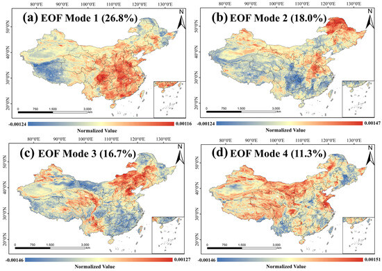
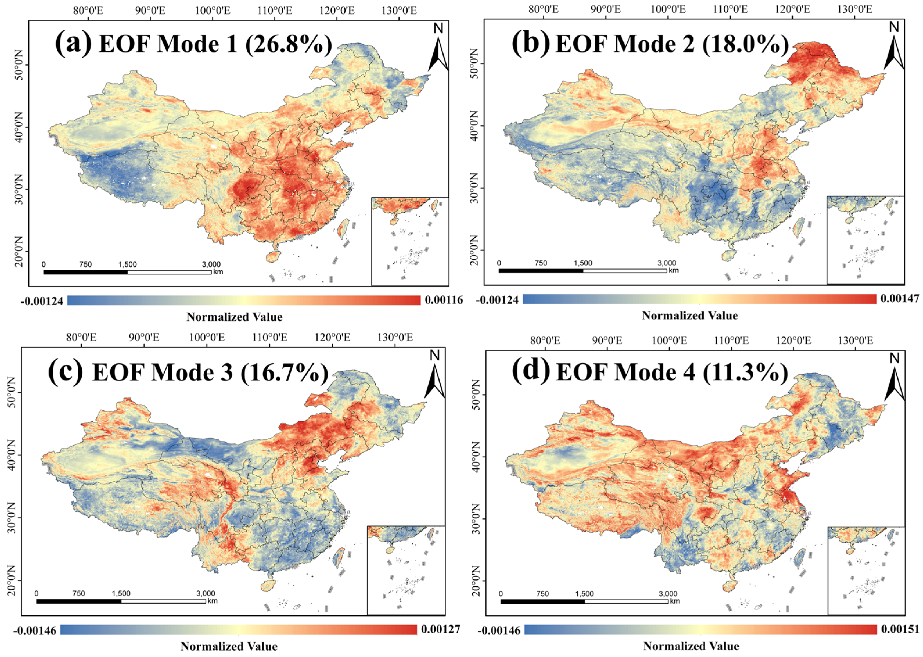
EOF decomposition was applied to the ΔXCO2 data over China from 2015 to 2022, revealing four dominant modes. As shown in Figure 5, the first mode exhibits a spatial pattern characterized by “positive anomalies in the southeast and negative anomalies in the northwest,” closely aligning with population density and economic activity intensity. This intuitively reflects the spatial trade-off relationship between anthropogenic carbon emissions and natural ecosystem uptake. Its corresponding time coefficient (PC1) was predominantly in a negative phase before 2019, indicating relatively dominant natural uptake or limited growth in anthropogenic emissions. However, a significant turning point occurred in 2020, with PC1 entering a sustained positive phase. This critical shift may be closely related to a phase transition of the Pacific Decadal Oscillation (PDO) [37] and the decline in aerosol optical depth resulting from air pollution control measures [38]. Together, these factors have made the anthropogenic emission signal increasingly prominent in regional XCO2 anomalies.
Figure 5.
Results of empirical orthogonal function (EOF) analysis for ΔXCO2 over China from 2015 to 2022.
The second mode manifests as a dipole structure with opposing phases between the north and south. Its formation is closely linked to the interannual variability of the East Asian summer monsoon [39]. PC2 exhibits strong interannual oscillations; for instance, a strong negative anomaly occurred in 2018 (following a weak El Niño), corresponding to a more southerly summer monsoon and enhanced net carbon sinks in the south. Conversely, a strong positive anomaly appeared in 2021 (a strong La Niña year), associated with intensified monsoon circulation and altered hydrothermal conditions in the north [40]. Essentially, this mode results from the monsoon’s influence on surface carbon flux dynamics by modulating regional hydrothermal patterns [41].
The third and fourth modes contribute relatively less to the total variance but reveal important processes at local scales. The third mode concentrates on anomalous signals in the Beijing–Tianjin–Hebei region and Yunnan Province. Its isolated high value in 2017 may be related to stagnant weather events and the transport of cross-border biomass burning emissions [42]. The fourth mode presents a spatial structure characterized by “negative in the southeast and positive in the northwest,” demarcated by the “Hu Line.” This can be viewed as a fundamental geographical background field reflecting differences in underlying surface properties and human activities between eastern and western China.
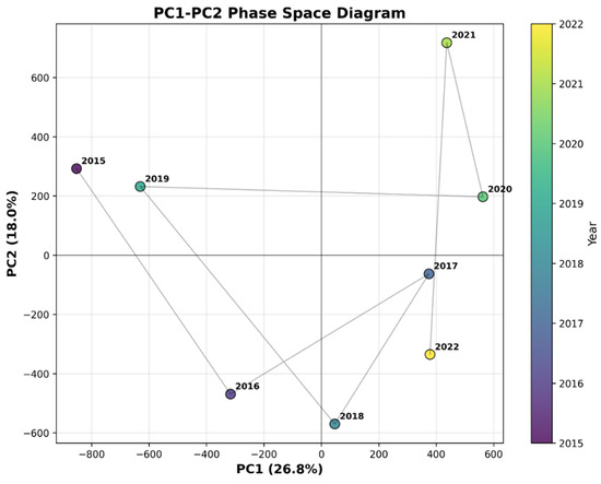
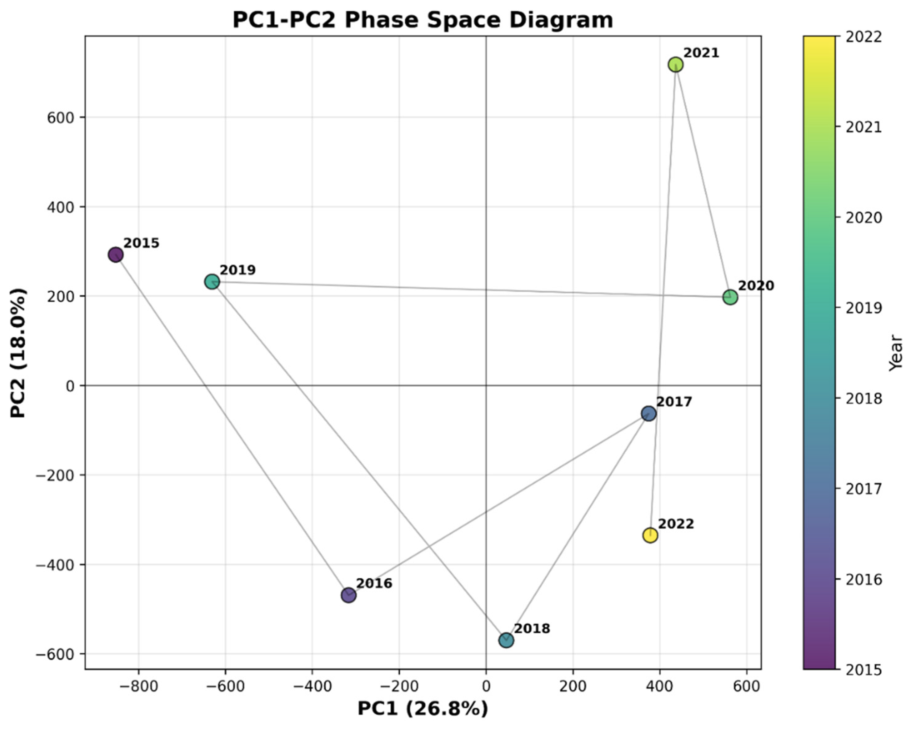
Notably, as illustrated in Figure 6, the period 2020–2021 constitutes a critical window characterized by dual-mode synergistic enhancement. During this period, the trend reversal in PC1 coincided with a strong positive phase in PC2. This simultaneous occurrence led to the superposition of positive anomalies from the first and second modes over North China, eliciting strong positive XCO2 anomalies [43]. In contrast, in South China, the first mode was positive while the second mode was negative, resulting in partial cancelation and less significant anomalous signals. This framework provides a mechanistic explanation for the observed high XCO2 anomalies in eastern China during this period. The turning point in PC1 may be coupled with the complex influences of post-pandemic economic recovery and energy structure transformation [44,45], while the oscillation in PC2 is likely primarily influenced by the El Niño–Southern Oscillation (ENSO).
Figure 6.
Spatial phase diagram of PC1–PC2 modes.
3.3. Regional Anthropogenic Emission Increments of XCO2
3.3.1. Anthropogenic XCO2 Emission Increments in Urban Agglomerations
We focused on regional XCO2 anomalies caused by anthropogenic emissions within China’s urban agglomeration areas, selecting the three major urban agglomerations of Beijing–Tianjin–Hebei (BTH), the Yangtze River Delta (YRD), and the Pearl River Delta (PRD) as typical anthropogenic emission source areas. These three regions serve as the core engines of China’s economic development, accounting for over 40% of the national economic output [46], and their carbon emission characteristics are representative for understanding China’s regional carbon cycle and anthropogenic impacts.
Based on the LISA framework introduced in Section 2.2.3, we first calculated the Local Moran’s I for TAF-XCO2 data across the three major urban agglomerations. A significance level of p ≤ 0.05 was adopted, corresponding to a 95% confidence interval (critical value |Z| = 1.96). Only spatial units whose Local Moran’s I Z-score exceeded this statistical threshold were assigned to one of the four spatial association categories, thereby ensuring the robust identification of high–high (HH) clusters indicative of regional XCO2 anomalies [47]. Concurrently, a dynamic background concentration curve was constructed by applying a quadratic polynomial fit to the latitudinal means of low–low (LL) cluster values. Local anthropogenic CO2 increments (dXCO2) were subsequently derived using Equations (1)–(8).
As summarized in Table 3, the multi-year mean dXCO2 values attributable to anthropogenic emissions for the period 2015–2019 were 3.46 ± 0.45 ppm for the Beijing–Tianjin–Hebei (BTH) region, 1.30 ± 0.36 ppm for the Yangtze River Delta (YRD), and 0.08 ± 0.14 ppm for the Pearl River Delta (PRD) (uncertainties expressed as 1σ). These results reveal a distinct spatial pattern wherein the anthropogenic emission contribution from the northern heavy industrial region is markedly higher than that of the southern coastal economic zones [48,49], with notably greater uncertainty observed in the PRD—a region characterized by a relatively low emission–concentration overlap ratio. In terms of seasonal variation, winter mean dXCO2 values for the three regions were 0.60 ppm, 0.78 ppm, and 0.61 ppm, respectively, while summer mean values were 0.94 ppm, 0.16 ppm, and 0.50 ppm. Further analysis indicates a pronounced enhancement of the anthropogenic contribution during summer in the BTH region. This pattern not only reflects persistently high emission intensity during the warm, high-energy-consumption season but may also be associated with the region’s distinctive vegetation cover characteristics—specifically, the vigorous summer vegetation regrowth may lead to an underestimation of background CO2 concentrations, thereby amplifying the apparent increment attributed to anthropogenic emissions [50].
Table 3.
Regional characteristic statistics for the Beijing–Tianjin–Hebei, Yangtze River Delta, and Pearl River Delta regions before and during the COVID-19 pandemic (Unit: ppm).
Dividing the study period into pre-pandemic (2015–2019) and pandemic (2020–2022) phases, comparative statistics for regional mean CO2 concentration and mean dXCO2 were compiled and are summarized in Table 3. The data show that during the pandemic, the annual mean dXCO2 in the BTH region decreased from 3.46 ppm to 2.28 ppm, and in the YRD from 1.30 ppm to 1.16 ppm. This phenomenon indicates a reduction in human activity intensity in these regions during the pandemic, consistent with global trends [51,52]. Conversely, the PRD experienced an increase from 0.08 ppm to 0.28 ppm, reflecting changes in regional emission structures and a trend of enhanced local anthropogenic emissions.
Comparison of winter dXCO2 further reinforces this spatial differentiation: during the pandemic, the mean winter dXCO2 in the BTH region reached 2.92 ppm, significantly higher than in the YRD (1.81 ppm) and PRD (0.40 ppm). This highlights that the northern industrial zone maintained relatively high emission levels even under the impact of the pandemic, demonstrating greater continuity and emission inertia in anthropogenic activities [53].
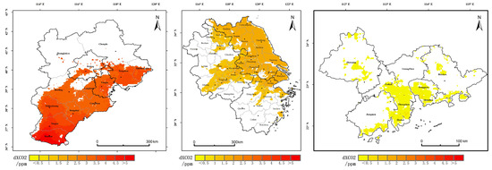
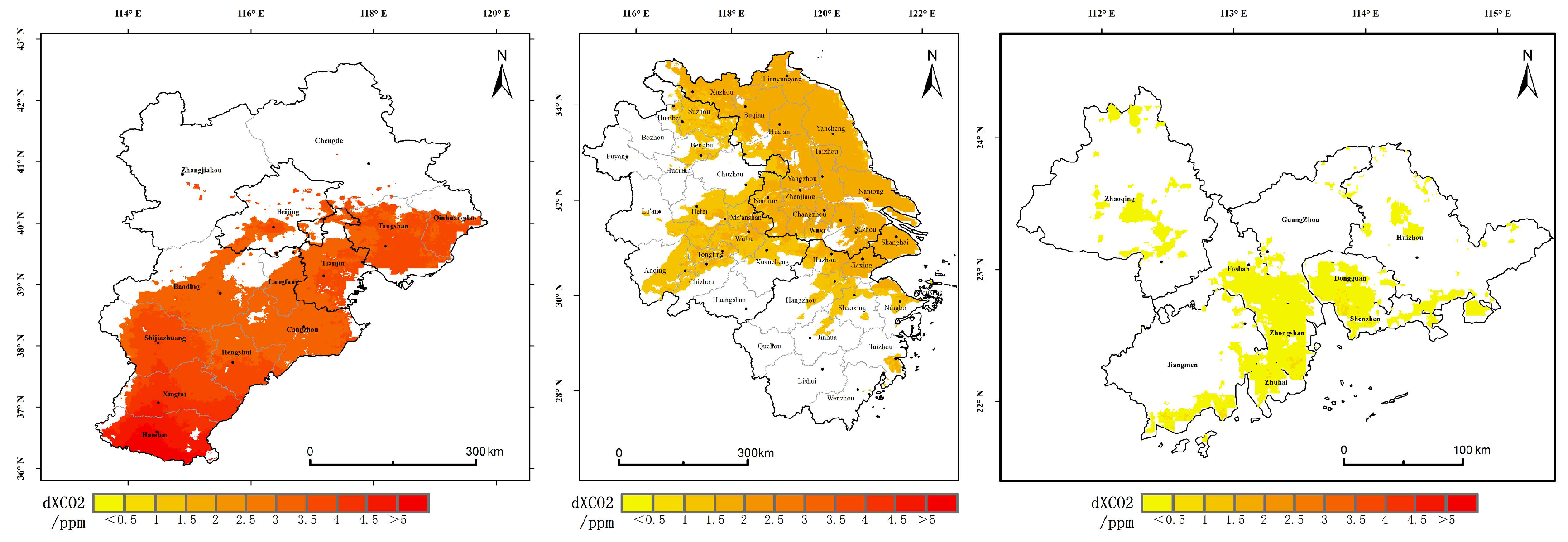
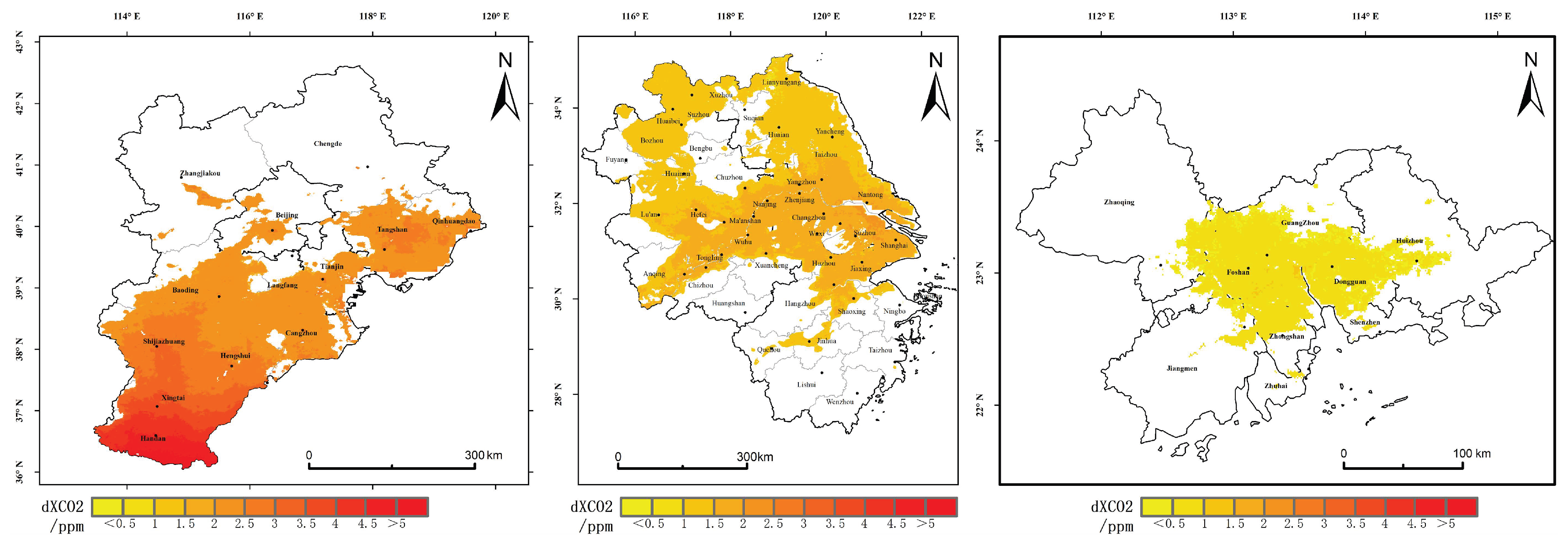
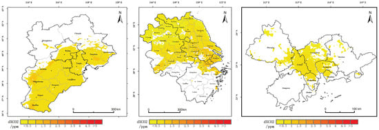
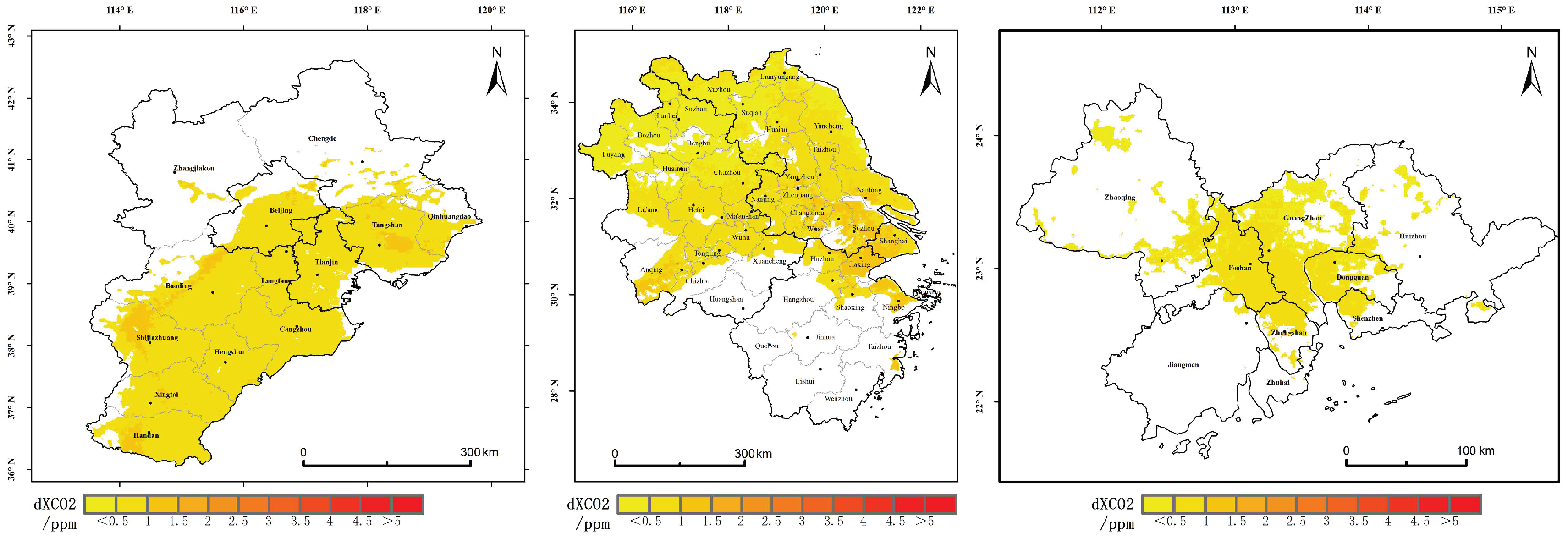
Supported by spatial autocorrelation analysis, High–High (HH) agglomeration areas of XCO2 anomalies were identified in each region. As shown in Figure 7, during the period 2015–2019, anomalous high-value areas in the BTH region were mainly distributed in Handan and Xingtai cities, located at the intersection of Hebei, Shanxi, Henan, and Shandong provinces, with local increments ranging from 2.95 to 5.74 ppm. The industrial structure of this area is dominated by heavy industries characterized by high pollution and high energy consumption, where vegetation uptake plays a negligible regulatory role, and anthropogenic emissions are predominant [54]. In the YRD, anomalous high-value areas were concentrated in Suzhou, Wuxi, Shanghai, and Jiaxing, with increments between 1.26 and 2.77 ppm, indicating the significant contribution of high-density economic activities to carbon emissions. Anomalous high-value areas in the PRD were primarily located in Shenzhen, Zhongshan, Zhuhai, Dongguan, and southern Jiangmen, with increments ranging from 0.06 to 1.05 ppm, corresponding to its high-intensity urban activities and energy consumption.
Figure 7.
Monitoring results of local XCO2 increments in HH (High–High) clusters of different urban agglomerations from 2015 to 2019.
As shown in Figure 8, entering the 2020–2022 period, the high-value areas in the BTH region remained concentrated in Handan and Xingtai, with increments slightly decreasing but still maintained between 1.79 and 5.57 ppm, suggesting that despite the pandemic’s impact, the fundamental emission pattern did not undergo radical change. In the PRD, the center of gravity for high-value areas shifted towards Guangzhou and Foshan, with increments rising to a range of 0.26–1.12 ppm. This may be associated with the surge in production of pandemic prevention materials and the consequent rise in energy consumption in related industries during the health crisis [55]. The distribution of high-value areas in the YRD showed relatively minor changes, with increments ranging from 0.81 to 2.44 ppm, indicating that this region was less severely affected by the pandemic and its economic activities possessed a certain degree of resilience.
Figure 8.
Monitoring results of local XCO2 increments in HH (High–High) clusters of different urban agglomerations from 2020 to 2022.
In summary, the XCO2 anomalies in the BTH, YRD, and PRD urban agglomerations exhibit significant regional differences and temporal evolution characteristics, revealing the complex modulating effects of varying economic development models, industrial structures, and pandemic disruptions on anthropogenic carbon emissions [56]. These findings provide important empirical evidence for understanding the spatial patterns and driving mechanisms of carbon emissions in China’s urban agglomeration regions.
3.3.2. Response of Anthropogenic Emission Increments During the COVID-19 Lockdown Period
Since December 2019, the novel coronavirus (COVID-19) pandemic has spread across numerous countries globally. To contain the virus, China implemented stringent lockdown measures that significantly reduced the intensity of human activities, consequently leading to a substantial decline in CO2 emissions [57,58]. This reduction was particularly pronounced in the early stages of the lockdown. Research by Wang Rong et al. indicated that by the end of February 2020, China’s CO2 emissions had decreased by approximately 23% year-on-year [57]. Buchwitz et al. conducted a preliminary investigation into XCO2 concentration changes in East China, observing a decrease of roughly 0.1–0.2 ppm [59]. Nevertheless, systematic quantitative analyses of changes in anthropogenic CO2 emission increments throughout the entire lockdown period remain insufficient, underscoring a critical research gap.
To address this, our study compared regional XCO2 anomalies between January and April 2020 and the corresponding months in 2015–2019. The results indicate that, compared to the same period in previous years, XCO2 anomalies in the YRD region showed a marginal decrease of approximately 0.07 ppm. In contrast, no significant decline was observed in the BTH and PRD regions. The resilience in the BTH region is likely attributable to its rigid industrial structure, dominated by thermal power, steel, and combined heat and power generation, which was less susceptible to pandemic-induced disruptions. Furthermore, extended periods of residential stay during the lockdown likely increased energy consumption for winter heating [60], thereby offsetting emission reductions from the transportation sector. In the PRD region, the sustained operation of core urban functions in these high-density cities generated rigid carbon emissions, particularly evident in the strengthening of the “water–energy–carbon” nexus [61].
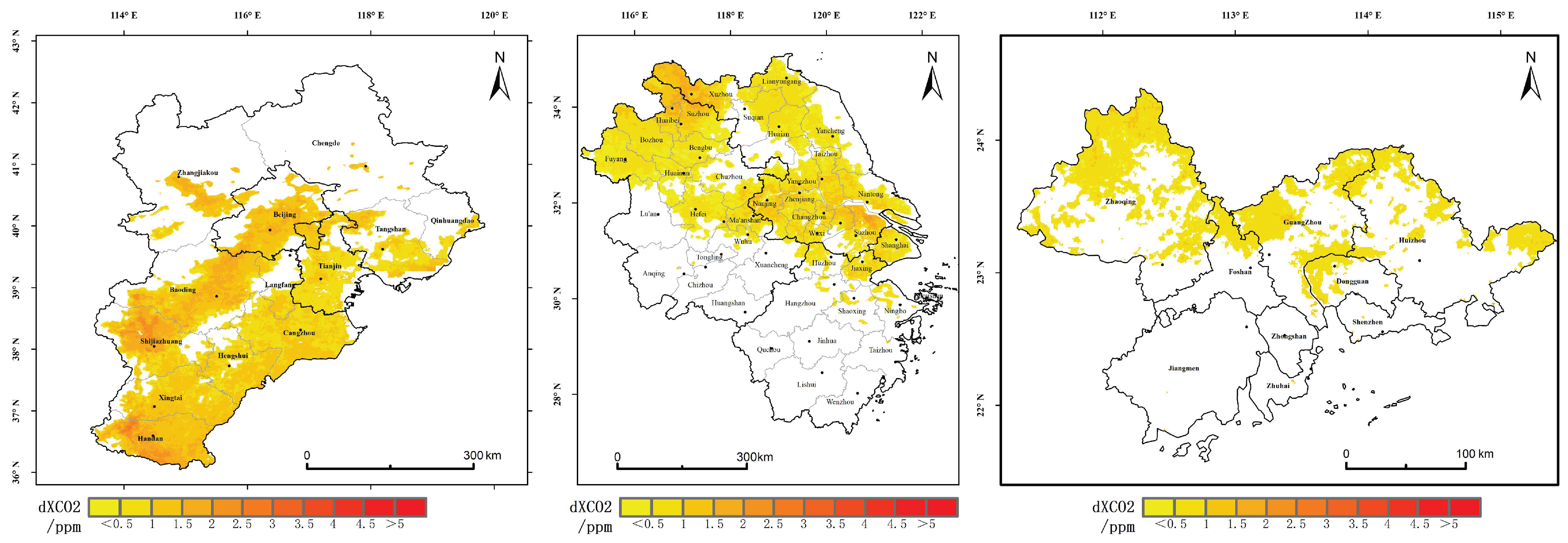
To further elucidate the differential responses of dXCO2 to emission reduction measures across the Beijing–Tianjin–Hebei (BTH), Yangtze River Delta (YRD), and Pearl River Delta (PRD) regions, this study compared dXCO2 anomalies during 2020 with those of the corresponding months in the 2015–2019 baseline period. As shown in Figure 9 and Figure 10, the results reveal a nuanced pattern: in the YRD region, the overall dXCO2 difference was approximately −0.01 ppm, yet a positive anomaly of 0.1 ppm persisted in areas of intensive human activity (High–High clusters), indicating that emissions in these core zones remained unabated even as regional totals declined. In the BTH region, overall dXCO2 increased by 0.13 ppm, with High–High clusters exhibiting a substantial rise of 0.37 ppm, corresponding to increases of 22% region-wide and 45% within the clusters. The PRD region also experienced increases, with overall dXCO2 rising by 0.07 ppm and High–High clusters by 0.09 ppm, reflecting gains of 23% and 15%, respectively. These divergent patterns underscore the considerable regulatory influence of spatial heterogeneity in industrial structure, energy consumption patterns, and human activity intensity on CO2 emission dynamics [61].
Figure 9.
Monitoring results of local XCO2 increments in HH (High–High) clusters of different urban agglomerations during the lockdown period from January to April 2020.
Figure 10.
Monitoring results of local XCO2 increments in HH (High–High) clusters of different urban agglomerations from January to April, averaged over 2015–2019.
Furthermore, this study evaluated dXCO2 concentration changes at the provincial administrative level. Within the BTH region, dXCO2 in Hebei Province increased by 0.12 ppm (approximately 22%), in Tianjin Municipality by 0.11 ppm (approximately 15%), and in background areas by 0.27 ppm (approximately 38%). In the YRD region, dXCO2 decreased by 0.02 ppm (approximately 3%) in Jiangsu Province, by 0.07 ppm (approximately 18%) in Anhui Province, by 0.1 ppm (approximately 41%) in Zhejiang Province, and by 0.29 ppm (approximately 30.57%) in Shanghai Municipality. The inter-provincial variations in dXCO2 change magnitude are likely closely associated with differences in industrial composition, population mobility patterns, and energy consumption characteristics [62].
4. Discussion
Accurately detecting anthropogenic CO2 increments in urban agglomerations is a scientific foundation for achieving regionally differentiated emission reduction. However, this study indicates that this detection process still faces multiple challenges related to mechanisms of natural interference and regional heterogeneity, which affect the reliable identification of incremental signals.
First, the inherent uncertainty of the data source constrains, to a certain extent, the applicability of the method in specific regions. During model training, the OCO-2 and OCO-3 satellite observations corresponding to TCCON sites were not excluded a priori; instead, a random partitioning strategy was adopted for constructing the training and validation sets in the three-fold cross-validation procedure, which introduces a degree of opacity. Moreover, not all satellite data overlying the TCCON sites were removed. This data handling strategy may give rise to certain errors. Although the TAF-XCO2 dataset employed in this study exhibits relatively high accuracy over eastern urban agglomerations, the discrimination of grid-scale XCO2 anomalies in western China remains subject to non-negligible uncertainty due to the absence of effective constraints from TCCON ground-based validation stations. Spatial overlay analysis further reveals pronounced interannual fluctuations in the degree of spatial correspondence between EDGAR emission inventory hot pixels and CO2 concentration hot pixels at the national scale. This phenomenon may be attributed, on the one hand, to the inherent limitations of relying on a single emission inventory dataset and, on the other, to the significant modulation exerted by large-scale environmental factors such as variations in atmospheric diffusion conditions and interannual variability of natural carbon sinks [63]. The above findings indicate that hot pixel detection methods predicated solely on concentration fields possess certain limitations in regions characterized by spatially dispersed emission sources or favorable atmospheric diffusion conditions.
Second, anthropogenic increments exhibit significant seasonal perturbation characteristics. The dXCO2 values in all three major urban agglomerations show pronounced seasonal differences, which are not entirely consistent with seasonal expectations of anthropogenic emissions. Taking the Beijing–Tianjin–Hebei region as an example, the summer increment is higher than the winter increment, presenting a phenomenon of “higher values in summer and lower values in winter.” This may be related to improved boundary layer diffusion conditions in summer and the enhanced uptake by vegetation carbon sinks in background areas, which lowers background concentrations. This reflects the difficulty in completely eliminating the seasonal dynamic influence of natural carbon sinks from current LL background areas, and separating vegetation signals from observational data remains a technical challenge [64].
Furthermore, regional industrial structure exerts a profound influence on the response mechanisms of anthropogenic emissions [65,66,67]. The differential dXCO2 responses during the COVID-19 lockdown period further validate this judgment. In particular, the increase in HH areas of the Beijing–Tianjin–Hebei region reached as high as 45%, reflecting the superimposed effect of rigid demand from heavy chemical industries and heating requirements; the increase in the Yangtze River Delta was only 16%, reflecting the greater emission resilience of its core cities; while the Pearl River Delta experienced an overall increase, possibly related to the surge in production of pandemic prevention materials. This finding indicates that under short-term anthropogenic perturbations, the CO2 increment response of urban agglomerations is highly constrained by local industrial structure characteristics. Future research should introduce region-specific factors to improve the applicability of unified models.
Regarding the independence of dXCO2 and methodological limitations, it is important to note that the TAF-XCO2 seamless dataset used in this study to extract anthropogenic increments incorporated fossil fuel emissions and NO2 as environmental covariates during the reconstruction process. Consequently, the resulting spatial distribution field of XCO2 unavoidably embeds some spatial patterns derived from the prior emission information. As demonstrated by Lei, Kiel, and their colleagues, spatial biases in prior emission estimates have a non-negligible influence on both simulated and observe d XCO2 enhancements [68,69,70]. Therefore, the dXCO2 derived using the LISA method in this study should be interpreted as a composite indicator that integrates satellite observations with the spatial patterns of prior emissions, rather than a pure observation-based increment entirely independent of emission inventories. Although this indicator has advantages in capturing the spatial structure and relative intensity of anthropogenic emissions, its absolute magnitude is, to some extent, influenced by the spatial allocation of the input prior information. Nonetheless, the annual modeling strategy adopted in this study means that the interannual variability of XCO2 depends more strongly on changes in the OCO satellite measurements themselves, which alleviates this limitation to a certain degree. In future work, we will further introduce purely observation-based fusion products that do not rely on emission priors, or statistical interpolation products based on in situ measurements, as benchmarks to more thoroughly and scientifically isolate the spatial anthropogenic increment signal.
Finally, it should be noted that this study did not explicitly quantify the spatiotemporal propagation of reconstruction errors when applying the TAF-XCO2 dataset to EOF and LISA analyses. Validation against TCCON ground-based stations only reflects accuracy at the point scale, whereas the uncertainty in dXCO2, as a differential quantity, is susceptible to both the selection strategy of the background field and the accumulation of errors. Consequently, the quantitative values of dXCO2 should be interpreted with caution in western regions where training samples are sparse. Future investigations will incorporate ensemble simulations or Bayesian frameworks to systematically assess the potential interference of these uncertainties on downstream analytical conclusions.
Accurately identifying anthropogenic CO2 increments in urban agglomerations remains challenged by seasonal interference and regional heterogeneity. Future efforts should focus on multi-source data fusion and the integration of Gaussian plume models with WRF-Chem simulations to establish localized background field models. Such advances will enhance the precision of increment detection and improve the generalizability of the analytical framework across diverse regions.
5. Conclusions
This study systematically analyzed the spatiotemporal variation characteristics of XCO2 over China based on the TAF-XCO2 dataset from January 2015 to December 2022, and further identified regional XCO2 anomalies induced by anthropogenic emissions.
The results indicate that at the national scale, XCO2 anomalies exhibit a spatial pattern characterized by “positive anomalies in the southeast and negative anomalies in the northwest,” which is highly consistent with population density distribution and economic activity intensity. On a seasonal scale, XCO2 displays a periodic pattern of “higher values in winter and lower values in summer,” reflecting the combined effects of enhanced emissions from winter heating and increased vegetation photosynthetic uptake in summer. EOF decomposition further extracted four dominant modes: the first mode represents the spatial trade-off relationship between anthropogenic emissions and natural uptake, with its time coefficient undergoing a significant turning point around 2020, possibly related to a phase transition of the Pacific Decadal Oscillation and the decline in aerosol optical depth; the second mode exhibits a north–south dipole spatial structure, significantly modulated by the interannual variability of the East Asian summer monsoon; the third and fourth modes correspond to local-scale influences from localized emission events and the fundamental geographical background, respectively.
In the regional-scale analysis, we proposed a method for identifying regional anthropogenic CO2 increments based on Local Indicators of Spatial Association (LISA), successfully extracting anthropogenic emission hotspot areas and their background concentrations for the three major urban agglomerations of Beijing–Tianjin–Hebei, the Yangtze River Delta, and the Pearl River Delta. The results show that during 2015–2019, the multi-year mean anthropogenic CO2 increments (dXCO2) for the three urban agglomerations were 3.46 ± 0.45 ppm, 1.3 ± 0.36 ppm, and 0.08 ± 0.14 ppm, respectively, revealing a spatial distribution pattern where the northern heavy industrial region exhibits significantly higher values than the southern coastal economic zones. During the 2020–2022 period, dXCO2 in the Beijing–Tianjin–Hebei region decreased to 2.28 ± 0.73 ppm, slightly decreased to 1.16 ± 0.43 ppm in the Yangtze River Delta, and increased to 0.28 ± 0.27 ppm in the Pearl River Delta, reflecting the differential responses of regional industrial structures and emission resilience to pandemic disruptions. It is noteworthy that in some years, summer anthropogenic CO2 increments were even higher than those in winter, indicating that current estimation methods based on background fields still struggle to completely eliminate the seasonal dynamic influence of natural carbon sinks. During the COVID-19 lockdown period, compared to historical periods, anthropogenic CO2 increments showed a slight decrease in the Yangtze River Delta, while slight increases were observed in the Beijing–Tianjin–Hebei and Pearl River Delta regions, suggesting that differences in regional industrial structure are key factors influencing anthropogenic CO2 increments.
This study provides a new analytical approach for identifying anthropogenic emission responses at national and regional scales using spatiotemporally continuous XCO2 datasets. The findings confirm that spatially continuous XCO2 datasets possess good potential for monitoring long-term XCO2 changes and identifying regional enhancement signals triggered by anthropogenic emissions, offering data support and methodological references for future greenhouse gas emission reduction assessments and policy formulation.
Author Contributions
W.Z.: algorithm implementation, data analysis, XCO2 interpretation, writing manuscripts; X.C.: research supervision, theoretical framework guidance; L.D.: revision of manuscripts, teamwork, innovative proposals, communication; X.X.: revision of manuscripts, teamwork, innovative proposals, communication; S.S.: revised manuscript; Q.Z.: Revising the manuscript. All authors have read and agreed to the published version of the manuscript.
Funding
This project was supported by the CAS National Comprehensive Research Project (Grant No. 072GJHZ2023098MI), the Tianshan Talent Project of Xinjiang Uygur Autonomous Region (Grant No. 2022TSYCLJ0056), and the Third Xinjiang Scientific Expedition Program (Grant No. 2021XJKK1300).
Data Availability Statement
The TAF-XCO2 seamless dataset used in this study is publicly available for free download via the Science Data Bank. This dataset provides monthly XCO2 over China from 2015 to 2022 at a spatial resolution of 0.01°, and can be accessed via the DOI: https://doi.org/10.57760/sciencedb.33694 (accessed on 13 March 2026). The EDGAR carbon emission inventory data cover the period from 2015 to 2022, with an annual temporal resolution and a spatial resolution of 0.1°, and are publicly available at https://aqmx.org (accessed on 14 March 2026). All other auxiliary datasets employed in the analyses and validation—including OCO-2/3 satellite retrievals, meteorological reanalysis data, vegetation indices, emission data, topographic data, among others—are publicly accessible. Detailed information and access methods for these datasets are provided in Table 1. All data can be obtained free of charge through their respective official channels or public data repositories.
Acknowledgments
During the preparation of this manuscript, the author(s) used Deepseek-R1 version to translate the manuscript into English. The authors have reviewed and edited the output and take full responsibility for the content of this publication.
Conflicts of Interest
The authors declare no competing interests.
Appendix A
Table A1.
Hyperparameter results of models for different years.
Figure A1.
Spatial distribution of mean CAMS XCO2 and mean ΔXCO2 in China from 2015 to 2022.
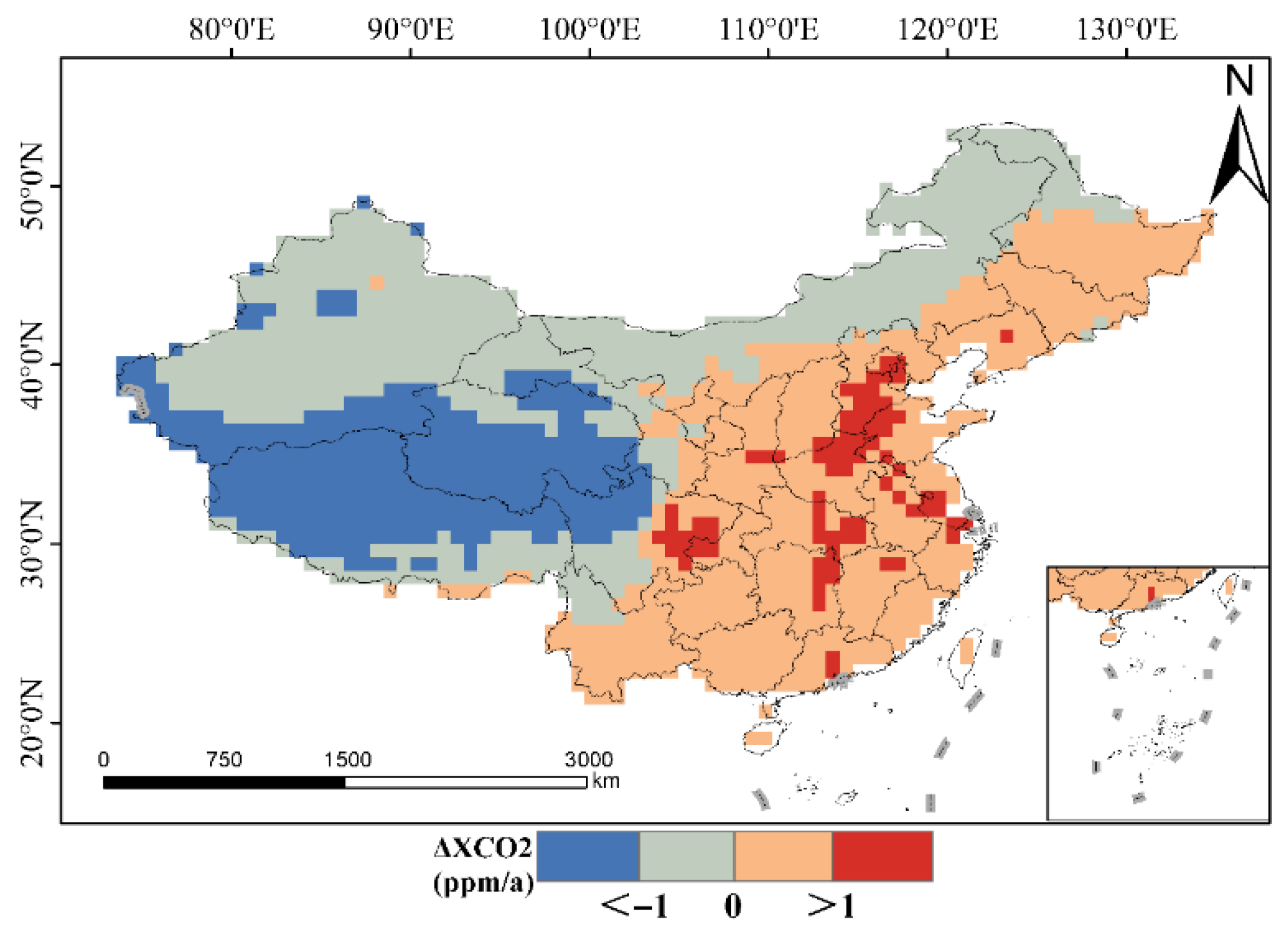
Figure A2.
Spatial distribution of seasonal CAMS ΔXCO2 from 2015 to 2022: (a) Winter and (b) Summer.
References
- Hegerl, G.C.; Brönnimann, S.; Cowan, T.; Friedman, A.R.; Hawkins, E.; Iles, C.; Müller, W.; Schurer, A.; Undorf, S. Causes of climate change over the historical record. Environ. Res. Lett. 2019, 14, 123006. [Google Scholar] [CrossRef] [Scilit]
- Ussiri, D.A.N.; Lal, R. Variability and Change in Climate. In Carbon Sequestration for Climate Change Mitigation and Adaptation; Springer: Cham, Switzerland, 2017; pp. 27–60. [Google Scholar]
- Song, S.; Tan, H.; Zhang, Y.; Ma, Y. A multiscale analysis of the relationship between urbanization and CO2 emissions using geo-weighted regression model. Discov. Sustain. 2024, 5, 113. [Google Scholar] [CrossRef] [Scilit]
- Gasser, T.; Boucher, O.; Lecocq, F.; Obersteiner, M. Trading-Off Emission Reduction, Carbon Capture and Geoengineering to Reach the Paris Agreement; American Geophysical Union: Washington, DC, USA, 2017; Volume 2017. [Google Scholar]
- Hakkarainen, J.; Ialongo, I.; Tamminen, J. Direct space-based observations of anthropogenic CO2 emission areas from OCO-2. Geophys. Res. Lett. 2016, 43, 11400–11406. [Google Scholar] [CrossRef] [Scilit]
- Schwandner, F.M.; Gunson, M.R.; Miller, C.E.; Carn, S.A.; Eldering, A.; Krings, T.; Verhulst, K.R.; Schimel, D.S.; Nguyen, H.M.; Crisp, D.; et al. Spaceborne detection of localized carbon dioxide sources. Science 2017, 358, eaam5782. [Google Scholar] [CrossRef] [Scilit] [PubMed]
- Sheng, M.; Hou, Y.; Song, H.; Ye, X.; Lei, L.; Ma, P.; Zeng, Z.-C. Estimating anthropogenic CO2 emissions from China’s Yangtze River Delta using OCO-2 observations and WRF-Chem simulations. Remote Sens. Environ. 2025, 316, 114515. [Google Scholar] [CrossRef] [Scilit]
- Ye, X.; Li, W.; Lauvaux, T.; Lin, S.; Zhang, Z.; Lin, Y.; Hua, J.; You, Q.; Lin, J. Constraining Anthropogenic Co2 Emissions Using Dense Observations from Oco-3: Disentangling Observed Imprints Over Xiamen-Zhangzhou-Quanzhou Metropolitan Area and Challenges. Urban Clim. 2025, 63, 102591. [Google Scholar] [CrossRef] [Scilit]
- Jin, C.; Xue, Y.; Yuan, T.; Zhao, L.; Jiang, X.; Sun, Y.; Wu, S.; Wang, X. Retrieval anthropogenic CO2 emissions from OCO-2 and comparison with gridded emission inventories. J. Clean. Prod. 2024, 448, 141418. [Google Scholar] [CrossRef] [Scilit]
- Xu, T.; Zhang, C.; Liu, C. Enhanced Quantification of Global Carbon Emitters Using Collocated OCO-3 CO2 and NO2 Observations From Twin Polar-Orbiting Satellites. Geophys. Res. Lett. 2025, 52, e2025GL116877. [Google Scholar] [CrossRef] [Scilit]
- Reuter, M.; Buchwitz, M.; Schneising, O.; Krautwurst, S.; O’Dell, C.W.; Richter, A.; Bovensmann, H.; Burrows, J.P. Towards monitoring localized CO2 emissions from space: Co-located regional CO2 and NO2 enhancements observed by the OCO-2 and S5P satellites. Atmos. Chem. Phys. 2019, 19, 9371–9383. [Google Scholar] [CrossRef] [Scilit]
- Zhang, W.; Chen, X.; Duan, L.; Song, S.; Zhou, Q. Construction of a 0.01° Monthly Seamless XCO2 Dataset over China: Based on a Temporally Adaptive Forest Model. Sci. Data 2026, Preprint. [Google Scholar]
- Eldering, A.; O’Dell, C.W.; Wennberg, P.O.; Crisp, D.; Gunson, M.R.; Viatte, C.; Avis, C.; Braverman, A.; Castano, R.; Chang, A.; et al. The Orbiting Carbon Observatory-2: First 18 months of science data products. Atmos. Meas. Tech. 2017, 10, 549–563. [Google Scholar] [CrossRef] [Scilit]
- Crisp, D.; Pollock, H.R.; Rosenberg, R.; Chapsky, L.; Lee, R.A.M.; Oyafuso, F.A.; Frankenberg, C.; O’Dell, C.W.; Bruegge, C.J.; Doran, G.B.; et al. The on-orbit performance of the Orbiting Carbon Observatory-2 (OCO-2) instrument and its radiometrically calibrated products. Atmos. Meas. Tech. 2017, 10, 59–81. [Google Scholar] [CrossRef] [Scilit]
- Taylor, T.E.; Eldering, A.; Merrelli, A.; Kiel, M.; Somkuti, P.; Cheng, C.; Rosenberg, R.; Fisher, B.; Crisp, D.; Basilio, R.; et al. OCO-3 early mission operations and initial (vEarly) XCO2 and SIF retrievals. Remote Sens. Environ. 2020, 251, 112032. [Google Scholar] [CrossRef] [Scilit]
- Taylor, T.E.; O’Dell, C.W.; Baker, D.; Bruegge, C.; Chang, A.; Chapsky, L.; Chatterjee, A.; Cheng, C.; Chevallier, F.; Crisp, D.; et al. Evaluating the consistency between OCO-2 and OCO-3 XCO2 estimates derived from the NASA ACOS version 10 retrieval algorithm. Atmos. Meas. Tech. 2023, 16, 3173–3209. [Google Scholar] [CrossRef] [Scilit]
- Olivier, J.G.; Bouwman, A.F.; van der Maas, C.W.; Berdowski, J.J. Emission database for global atmospheric research (Edgar). Environ. Monit. Assess. 1994, 31, 93–106. [Google Scholar] [CrossRef] [Scilit] [PubMed]
- Guizzardi, D.; Becker, W.; Pagani, F.; Muntean, M.; Crippa, M. Global up-to date emissions using the EDGAR Fast-Track methodology. Sci. Data 2025, 12, 1243. [Google Scholar] [CrossRef] [Scilit] [PubMed]
- Yang, L.; Luo, H.; Yuan, Z.; Zheng, J.; Huang, Z.; Li, C.; Lin, X.; Louie, P.K.K.; Chen, D.; Bian, Y. Quantitative impacts of meteorology and precursor emission changes on the long-term trend of ambient ozone over the Pearl River Delta, China, and implications for ozone control strategy. Atmos. Chem. Phys. 2019, 19, 12901–12916. [Google Scholar] [CrossRef] [Scilit]
- Zhou, L.; Zhang, J.; Lu, T.; Bao, M.; Deng, X.; Hu, X. Pollution patterns and their meteorological analysis all over China. Atmos. Environ. 2021, 246, 118108. [Google Scholar] [CrossRef] [Scilit]
- Zhan, C.; Xie, M.; Liu, J.; Wang, T.; Xu, M.; Chen, B.; Li, S.; Zhuang, B.; Li, M. Surface Ozone in the Yangtze River Delta, China: A Synthesis of Basic Features, Meteorological Driving Factors, and Health Impacts. J. Geophys. Res. Atmos. 2021, 126, e2020JD033600. [Google Scholar] [CrossRef] [Scilit]
- Jawson, S.D.; Niemann, J.D. Spatial patterns from EOF analysis of soil moisture at a large scale and their dependence on soil, land-use, and topographic properties. Adv. Water Resour. 2007, 30, 366–381. [Google Scholar] [CrossRef] [Scilit]
- Cox, T.F. Spatial Processes: Models and Applications. R. Stat. Soc. J. Ser. A Gen. 1984, 147, 515. [Google Scholar] [CrossRef] [Scilit]
- Fu, S.H.; Jha, P.; Gupta, P.C.; Kumar, R.; Dikshit, R.; Sinha, D. Geospatial Analysis on the Distributions of Tobacco Smoking and Alcohol Drinking in India. PLoS ONE 2014, 9, e102416. [Google Scholar] [CrossRef] [Scilit]
- Fu, W.J.; Jiang, P.K.; Zhou, G.M.; Zhao, K.L. Using Moran’s I and GIS to study the spatial pattern of forest litter carbon density in a subtropical region of southeastern China. Biogeosciences 2014, 11, 2401–2409. [Google Scholar] [CrossRef] [Scilit]
- Anselin, L. Local Indicators of Spatial Association—LISA. Geogr. Anal. 1995, 27, 93–115. [Google Scholar] [CrossRef] [Scilit]
- Sheng, M.Y. Response of Atmospheric CO2 Concentration Changes to Anthropogenic Emissions Using Multi-source Carbon Satellite Observations. Ph.D. Thesis, Aerospace Information Research Institude, Chinese Academy of Sciences, Beijing, China, 2022. [Google Scholar]
- Sheng, M.; Lei, L.; Zeng, Z.-C.; Rao, W.; Zhang, S. Detecting the Responses of CO2 Column Abundances to Anthropogenic Emissions from Satellite Observations of GOSAT and OCO-2. Remote Sens. 2021, 13, 3524. [Google Scholar] [CrossRef] [Scilit]
- Wei, W.; Yang, S.; Ma, L.; Xie, B.; Zhou, J.; Wang, M.; Wei, X.; Chen, D. Spatiotemporal variations of fossil fuel CO2 emissions in China: A sectoral allocation approach based on multi-source data. Environ. Pollut. 2024, 360, 124589. [Google Scholar] [CrossRef] [Scilit]
- Piao, S.; Huang, M.; Liu, Z.; Wang, X.; Ciais, P.; Canadell, J.G.; Wang, K.; Bastos, A.; Friedlingstein, P.; Houghton, R.A.; et al. Lower land-use emissions responsible for increased net land carbon sink during the slow warming period. Nat. Geosci. 2018, 11, 739–743. [Google Scholar] [CrossRef] [Scilit]
- Dong, X.; Yue, M.; Jiang, Y.; Hu, X.-M.; Ma, Q.; Pu, J.; Zhou, G. Analysis of CO2 spatio-temporal variations in China using a weather–biosphere online coupled model. Atmos. Chem. Phys. 2021, 21, 7217–7233. [Google Scholar] [CrossRef] [Scilit]
- Kulawik, S.S.; Crowell, S.; Baker, D.; Liu, J.; McKain, K.; Sweeney, C.; Biraud, S.C.; Wofsy, S.; O’Dell, C.W.; Wennberg, P.O.; et al. Characterization of OCO-2 and ACOS-GOSAT biases and errors for CO2 flux estimates. Atmos. Meas. Tech. Discuss. 2019, preprint. [Google Scholar]
- Zhang, H.; Guo, W.; Wang, S.; Yao, Z.; Lv, L.; Teng, Y.; Li, X.; Shen, X. Insights into the spatiotemporal heterogeneity, sectoral contributions and drivers of provincial CO2 emissions in China from 2019 to 2022. J. Environ. Sci. 2025, 155, 510–524. [Google Scholar] [CrossRef] [Scilit] [PubMed]
- Chen, X.; Zhang, S.; Lin, J.; Tian, J.; Ma, X. Temporal and spatial evolution of interprovincial CO2 emissions and driving factors based on a spatial-temporal geo-weighted regression mode. Front. Clim. 2025, 7, 1649791. [Google Scholar] [CrossRef] [Scilit]
- Kumar, P.; Sharan, M. Parameterization of the eddy diffusivity in a dispersion model over homogeneous terrain in the atmospheric boundary layer. Atmos. Res. 2012, 106, 30–43. [Google Scholar] [CrossRef] [Scilit]
- Xia, L.; Liu, R.; Fan, W.; Ren, C. Emerging carbon dioxide hotspots in East Asia identified by a top-down inventory. Commun. Earth Environ. 2025, 6, 10. [Google Scholar] [CrossRef] [Scilit]
- Li, S.; Wu, L.; Yang, Y.; Geng, T.; Cai, W.; Gan, B.; Chen, Z.; Jing, Z.; Wang, G.; Ma, X. The Pacific Decadal Oscillation less predictable under greenhouse warming. Nat. Clim. Chang. 2020, 10, 30–34. [Google Scholar] [CrossRef] [Scilit]
- Yeh, S.-W.; Kim, W.-M.; Kim, Y.H.; Moon, B.-K.; Park, R.J.; Song, C.-K. Changes in the variability of the North Pacific sea surface temperature caused by direct sulfate aerosol forcing in China in a coupled general circulation model. J. Geophys. Res. 2013, 118, 1261–1270. [Google Scholar] [CrossRef] [Scilit]
- Huang, Y.L.; Chen, H.S.; Jiang, W.; Xu, B.; Li, Z.X. Multi-spatial modes of East Asian summer monsoon activity: Comparative analysis of various reanalysis data. Chin. J. Atmos. Sci. 2015, 39, 145–160. (In Chinese) [Google Scholar]
- Cui, L.L.; Shi, J.; Xiao, F.J. Impacts of climatic factors and EI Nino/La Nina events on the changes of terrestrial ecosystem NPP in China. Acta Geogr. Sin. 2018, 73, 54–66. [Google Scholar]
- Yi, C.; Pendall, E.; Ciais, P. Focus on extreme events and the carbon cycle. Environ. Res. Lett. 2015, 10, 070201. [Google Scholar] [CrossRef] [Scilit]
- Huang, X.; Ding, A.; Wang, Z.; Ding, K.; Gao, J.; Chai, F.; Fu, C. Amplified transboundary transport of haze by aerosol–boundary layer interaction in China. Nat. Geosci. 2020, 13, 428–434. [Google Scholar] [CrossRef] [Scilit]
- Yang, K.; Cai, W.; Huang, G.; Hu, K.; Ng, B.; Wang, G. Increased variability of the western Pacific subtropical high under greenhouse warming. Proc. Natl. Acad. Sci. USA 2022, 119, e2120335119. [Google Scholar] [CrossRef] [Scilit] [PubMed]
- Fu, Y.; Sun, W.; Luo, F.; Zhang, Y.; Zhang, X. Variation patterns and driving factors of regional atmospheric CO2 anomalies in China. Environ. Sci. Pollut. Res. 2022, 29, 19390–19403. [Google Scholar] [CrossRef] [Scilit] [PubMed]
- Lu, W.; Li, X.; Li, S.; Cheng, T.; Guo, Y.; Fang, W. Effects of Emission Variability on Atmospheric CO2 Concentrations in Mainland China. Remote Sens. 2025, 17, 814. [Google Scholar] [CrossRef] [Scilit]
- Fang, C.L. China’s Urban Agglomeration and Metropolitan Area Construction Under the New Development Pattern. Econ. Geogr. 2021, 41, 1–7. [Google Scholar]
- Getis, A.; Ord, J.K. The Analysis of Spatial Association by Use of Distance Statistics. In Perspectives on Spatial Data Analysis; Anselin, L., Rey, S.J., Eds.; Springer: Berlin/Heidelberg, Germany, 2010; pp. 127–145. [Google Scholar]
- Shan, Y.; Guan, D.; Zheng, H.; Ou, J.; Li, Y.; Meng, J.; Mi, Z.; Liu, Z.; Zhang, Q. China CO2 emission accounts 1997–2015. Sci. Data 2018, 5, 170201. [Google Scholar] [CrossRef] [Scilit] [PubMed]
- Zheng, B.; Tong, D.; Li, M.; Liu, F.; Hong, C.; Geng, G.; Li, H.; Li, X.; Peng, L.; Qi, J.; et al. Trends in China’s anthropogenic emissions since 2010 as the consequence of clean air actions. Atmos. Chem. Phys. 2018, 18, 14095–14111. [Google Scholar] [CrossRef] [Scilit]
- Lei, L.; Zhong, H.; He, Z.; Cai, B.; Yang, S.; Wu, C.; Zeng, Z.; Liu, L.; Zhang, B. Assessment of atmospheric CO2 concentration enhancement from anthropogenic emissions based on satellite observations. Chin. Sci. Bull. 2017, 62, 2941–2950. (In Chinese) [Google Scholar] [CrossRef] [Scilit]
- Le Quéré, C.; Jackson, R.B.; Jones, M.W.; Smith, A.J.P.; Abernethy, S.; Andrew, R.M.; De-Gol, A.J.; Willis, D.R.; Shan, Y.; Canadell, J.G.; et al. Temporary reduction in daily global CO2 emissions during the COVID-19 forced confinement. Nat. Clim. Chang. 2020, 10, 647–653. [Google Scholar] [CrossRef] [Scilit]
- Huang, C.; An, J.; Wang, H.; Liu, Q.; Tian, J.; Wang, Q.; Hu, Q.; Yan, R.; Shen, Y.; Duan, Y.; et al. Highly Resolved Dynamic Emissions of Air Pollutants and Greenhouse Gas CO2 during COVID-19 Pandemic in East China. Environ. Sci. Technol. Lett. 2021, 8, 853–860. [Google Scholar] [CrossRef] [Scilit]
- Xiang, C.; Li, R.; Liang, A.; Wang, J. Analysis of air pollutants concentration variations and human impact by remote sensing: Implications for sustainable urban air quality management. Sustain. Futures 2025, 10, 101019. [Google Scholar] [CrossRef] [Scilit]
- Wang, J.; Feng, L.; Palmer, P.I.; Liu, Y.; Fang, S.; Bösch, H.; O’Dell, C.W.; Tang, X.; Yang, D.; Liu, L.; et al. Large Chinese land carbon sink estimated from atmospheric carbon dioxide data. Nature 2020, 586, 720–723. [Google Scholar] [CrossRef] [Scilit]
- Department of Science and Technology of Guangdong Province. Statistical Bulletin on National Economic and Social Development of Guangdong Province. 2020. Available online: https://gdstc.gd.gov.cn/zwgk_n/sjjd/content/post_3517392.html (accessed on 6 March 2026).
- Jia, B.; Xie, M.; Wu, J.; Zhao, J. Towards low carbon urban agglomerations: Spatiotemporal characteristics and influencing factors of carbon emission intensity and network linkages in China’s urban agglomerations. Ecol. Indic. 2025, 177, 113728. [Google Scholar] [CrossRef] [Scilit]
- Wang, R.; Xiong, Y.; Xing, X.; Yang, R.; Li, J.; Wang, Y.; Cao, J.; Balkanski, Y.; Peñuelas, J.; Ciais, P.; et al. Daily CO2 Emission Reduction Indicates the Control of Activities to Contain COVID-19 in China. Innovation 2020, 1, 100062. [Google Scholar] [CrossRef] [Scilit]
- Zheng, B.; Geng, G.; Ciais, P.; Davis, S.J.; Martin, R.V.; Meng, J.; Wu, N.; Chevallier, F.; Broquet, G.; Boersma, F.; et al. Satellite-based estimates of decline and rebound in China’s CO2 emissions during COVID-19 pandemic. Sci. Adv. 2020, 6, eabd4998. [Google Scholar] [CrossRef] [Scilit]
- Buchwitz, M.; Reuter, M.; Noël, S.; Bramstedt, K.; Schneising, O.; Hilker, M.; Fuentes Andrade, B.; Bovensmann, H.; Burrows, J.P.; Di Noia, A.; et al. Can a regional-scale reduction of atmospheric CO2 during the COVID-19 pandemic be detected from space? A case study for East China using satellite XCO2 retrievals. Atmos. Meas. Tech. 2021, 14, 2141–2166. [Google Scholar] [CrossRef] [Scilit]
- Wang, Y.; Yuan, Z.; Yan, J.; Zhang, H.; Guan, Q.; Rao, S.; Jiang, C.; Duan, Z. Analysis of Synergistic Drivers of CO2 and NOX Emissions from Thermal Power Generating Units in Beijing–Tianjin–Hebei Region, 2010–2020. Sustainability 2024, 16, 7554. [Google Scholar] [CrossRef] [Scilit]
- Lin, G.; Jiang, D.; Yin, Y.; Fu, J. A carbon-neutral scenario simulation of an urban land–energy–water coupling system: A case study of Shenzhen, China. J. Clean. Prod. 2023, 383, 135534. [Google Scholar] [CrossRef] [Scilit]
- Shan, W.; Wang, Q.; Ma, Z.; Xu, X.; Cai, B.; Bo, X. Evidence of policy-driven emission reductions and post-pandemic rebound from high-resolution inventories in China. J. Environ. Sci. 2026, in press. [CrossRef] [Scilit]
- Banja, M.; Crippa, M.; Guizzardi, D.; Muntean, M.; Pagani, F.; Pisoni, E. A comparative analysis of EDGAR and UNFCCC GHG emissions inventories: Insights on trends, methodology and data discrepancies. Earth Syst. Sci. Data 2025, 17, 6461–6486. [Google Scholar] [CrossRef] [Scilit]
- Storm, I.; Karstens, U.; D’Onofrio, C.; Vermeulen, A.; Hammer, S.; Super, I.; Glauch, T.; Peters, W. Monitoring CO2 in diverse European cities: Highlighting needs and challenges through characterisation. Earth Syst. Sci. Data 2025, 17, 6681–6701. [Google Scholar] [CrossRef] [Scilit]
- Liu, Z.; Ciais, P.; Deng, Z.; Lei, R.; Davis, S.J.; Feng, S.; Zheng, B.; Cui, D.; Dou, X.; Zhu, B.; et al. Near-real-time monitoring of global CO2 emissions reveals the effects of the COVID-19 pandemic. Nat. Commun. 2020, 11, 5172. [Google Scholar] [CrossRef] [Scilit] [PubMed]
- Sikarwar, V.S.; Reichert, A.; Jeremias, M.; Manovic, V. COVID-19 pandemic and global carbon dioxide emissions: A first assessment. Sci. Total Environ. 2021, 794, 148770. [Google Scholar] [CrossRef] [Scilit]
- Pan, S. The short-term impacts of COVID-19 outbreak on carbon emissions: Causal evidence from China. Appl. Econ. Lett. 2025, 32, 263–269. [Google Scholar] [CrossRef] [Scilit]
- Lei, R.; Feng, S.; Danjou, A.; Broquet, G.; Wu, D.; Lin, J.C.; O'Dell, C.W.; Lauvaux, T. Fossil fuel CO2 emissions over metropolitan areas from space: A multi-model analysis of OCO-2 data over Lahore, Pakistan. Remote Sens. Environ. 2021, 264, 112625. [Google Scholar] [CrossRef] [Scilit]
- Lei, R.; Feng, S.; Xu, Y.; Tran, S.; Ramonet, M.; Grutter, M.; Garcia, A.; Campos-Pineda, M.; Lauvaux, T. Reconciliation of asynchronous satellite-based NO2 and XCO2 enhancements with mesoscale modeling over two urban landscapes. Remote Sens. Environ. 2022, 281, 113241. [Google Scholar] [CrossRef] [Scilit]
- Kiel, M.; Eldering, A.; Roten, D.D.; Lin, J.C.; Feng, S.; Lei, R.; Lauvaux, T.; Oda, T.; Roehl, C.M.; Blavier, J.F.; et al. Urban-focused satellite CO2 observations from the Orbiting Carbon Observatory-3: A first look at the Los Angeles megacity. Remote Sens. Environ. 2021, 258, 112314. [Google Scholar] [CrossRef] [Scilit]

Disclaimer/Publisher’s Note: The statements, opinions and data contained in all publications are solely those of the individual author(s) and contributor(s) and not of MDPI and/or the editor(s). MDPI and/or the editor(s) disclaim responsibility for any injury to people or property resulting from any ideas, methods, instructions or products referred to in the content. |
© 2026 by the authors. Licensee MDPI, Basel, Switzerland. This article is an open access article distributed under the terms and conditions of the Creative Commons Attribution (CC BY) license.