


Highlights
What are the main findings?
- A deep learning model (Att-ResUNetDEM) integrating attention mechanisms and digital elevation model (DEM) topographic data was developed based on FY-4A multi-channel satellite observations, achieving regionalized retrieval of dynamic tropopause pressure over the winter Tibetan Plateau, with MAE and RMSE improved by 13.2% and 9.2% respectively, and correlation coefficient raised to 0.76 compared to the random forest baseline.
- Incorporating DEM topographic constraints improved the meridional tropopause pressure gradient retrieval along the main aviation corridor (30°N, 90–104°E), raising the correlation coefficient from 0.80 to 0.87 and effectively suppressing error amplification in strong-gradient regions, significantly enhancing spatial gradient consistency.
What are the implications of the main findings?
- The regionalized, season-specific modeling strategy combined with embedded topographic information provides a new technical pathway for high-resolution dynamic tropopause monitoring over complex terrain and multi-circulation-influenced regions, supporting real-time assessment and early warning of clear-air turbulence risks along Tibetan Plateau aviation routes.
- This study demonstrates the superiority of deep learning frameworks in capturing spatially coherent tropopause gradient evolution under complex mid-latitude dynamical environments, establishing a methodological foundation for near-real-time geostationary satellite-based tropopause retrieval and regionalized modeling.
Abstract
The dynamical tropopause layer pressure (DTLP) represents a key interface characterizing upper-tropospheric stratification and atmospheric dynamical structure. Its spatial morphology and gradient variations directly influence jet stream distribution as well as the intensity and location of clear-air turbulence (CAT). Over the Tibetan Plateau, complex terrain and pronounced dynamical variability result in a significantly lower tropopause height and enhanced horizontal gradients during winter. Aircraft cruising altitudes frequently approach or intersect the tropopause layer in this region, making accurate and fine-scale characterization of DTLP structures critically important for aviation safety. A deep learning-based DTLP retrieval model (Att-ResUNetDEM) is developed by integrating terrain constraints and an attention mechanism. Using MERRA-2 reanalysis data as supervisory labels, the model incorporates a squeeze-and-excitation (SE) attention mechanism within a residual encoder–decoder framework, while a digital elevation model (DEM) is introduced as an additional input channel and fused with satellite brightness temperature data to explicitly account for terrain effects. A random forest (RF) model is implemented as a baseline for comparison. Compared with the RF model, the Att-ResUNetDEM reduces the MAE and RMSE by 13.20% and 9.19%, respectively, while increasing the correlation coefficient to 0.76. Over the primary aviation corridors of the Tibetan Plateau, the Att-ResUNetDEM model achieves a correlation coefficient(R) of 0.87, with markedly reduced gradient dispersion. A representative CAT case further confirms the model’s ability to capture the overall DTLP morphology and gradient enhancement zones. Overall, by combining a regionalized modeling strategy with terrain constraints, this study systematically improves DTLP retrieval accuracy and gradient consistency over complex terrain, providing a new technical pathway for high-resolution tropopause monitoring and aviation operation support.
1. Introduction
The tropopause serves as the physical boundary separating the moist, turbulently mixed troposphere from the dry and stably stratified stratosphere [1,2]. As a key “gateway” for energy and mass exchange between the troposphere and stratosphere [3,4,5], long-term variations in its thermal and dynamical structures are widely regarded as important indicators of climate change [6,7,8,9,10]. On synoptic time scales, anomalous tropopause structures—such as steepening or tropopause folding—can facilitate stratospheric air intrusion into the troposphere [11], accelerate cyclogenesis [12,13], potentially trigger severe mesoscale weather processes, including deep convection [14,15,16,17,18,19,20,21], and serve as important source regions for the upward propagation of gravity waves and planetary waves [22,23]. From the perspective of civil aviation operations, commercial air traffic is primarily concentrated near the tropopause level [24,25]. Tropopause pressure is not only a key reference parameter for cruise-level planning and convective cloud avoidance, but abrupt variations or folding structures of the tropopause are also major sources of (CAT) [26,27,28,29]. Accordingly, the International Civil Aviation Organization (ICAO) mandates that tropopause height be indicated on high-level significant weather charts.
Based on the pronounced thermodynamic, dynamical, and chemical discontinuities across the tropopause, its definitions are generally classified into two categories: thermodynamic and dynamical [30,31,32]. The lapse-rate tropopause (LRT), proposed by the World Meteorological Organization (WMO) in 1957, is the most widely used thermodynamic definition [33]. It defines the tropopause as the lowest level at which the lapse rate decreases to 2 °C km−1 or less, provided that the mean lapse rate within the 2 km layer above does not exceed 2 °C km−1. The LRT can be derived from radiosonde observations [34,35,36,37], Global Navigation Satellite System radio occultation (GNSS-RO) measurements [38,39,40], or reanalysis datasets [41]. However, the lapse rate is not a conserved quantity, and its identification accuracy is sensitive to seasonal variations, latitude, and complex atmospheric processes, such as tropopause folding and Rossby wave breaking events [42,43]. In subtropical transition regions, multiple secondary LRTs are often identified within a single temperature profile [44], making the determination of the primary LRT challenging [45]. Moreover, the LRT has limited capability in representing stratosphere–troposphere exchange and dynamical anomalies, and it cannot be directly linked to upper-level frontal systems and jet stream activity. To overcome these limitations, Reed proposed defining the dynamical tropopause using potential vorticity (PV) surfaces [46], which has since been widely applied in mid- and high-latitude regions, particularly in areas of strong cyclonic activity [42,47]. The dynamical tropopause layer pressure (DTLP) is commonly defined by the |PV| = 2 PVU surface (1 PVU = 10−6 K kg−1 m2 s−1) [3,48,49], although this threshold may be adjusted within the range of 1–5 PVU depending on geographical location, season, and synoptic conditions [46,50,51,52,53,54,55]. Since PV approaches zero in tropical regions due to weak absolute vorticity, some studies adopt a hybrid definition, using the LRT in the tropics and DTLP in extratropical regions [56,57]. Compared with the LRT, DTLP provides a more comprehensive representation of atmospheric stability, density, and rotational characteristics. Its structural variations are closely associated with upper-level frontal zones, jet streams, and tropopause folding processes [58,59,60], which are also the primary regions of clear-air turbulence (CAT) occurrence [27,61,62,63,64]. Therefore, high spatiotemporal resolution DTLP products are of substantial practical importance for aviation safety. This also constitutes the fundamental motivation for selecting DTLP as the target variable in this study.
The Tibetan Plateau, located at the intersection of the summer monsoon, winter monsoon, and winter westerlies, serves as an important global pathway for stratosphere–troposphere exchange [65,66] and plays a key role in the variability of the East Asian subtropical westerly jet [67]. Driven by the combined thermal and dynamical effects of complex topography, tropopause folding occurs frequently over this region, particularly in winter and spring, significantly enhancing both the frequency and intensity of CAT [59]. As a result, the Tibetan Plateau is recognized as one of the global hotspots of CAT occurrence [68]. However, current approaches for obtaining tropopause height mainly rely on radiosonde observations, aircraft measurements, and numerical reanalysis products [36,37,44,49,69], all of which exhibit notable limitations over the Tibetan Plateau. Radiosonde stations and flight routes are extremely sparse in this region, making it difficult to reconstruct the spatial structure of the tropopause [70]. Numerical models are further constrained by spatial resolution and computational cost, limiting their ability to capture the rapid evolution of tropopause structures at high temporal frequency and near-real-time scales. In contrast, geostationary meteorological satellites, with their high spatiotemporal resolution and wide coverage, provide a promising pathway for tropopause monitoring. Previous studies have utilized water vapor channel observations from geostationary satellites to identify tropopause folding and assess CAT risk, based on water vapor gradient characteristics or the dynamical linkage between potential vorticity (PV) and the tropopause [71,72,73,74,75]. Building upon these efforts, Shou et al. introduced statistical machine learning methods for DTLP retrieval using FY-4A multi-channel observations [76]. By comparing linear regression, K-nearest neighbors (KNN), gradient boosting decision trees (GBDT), and random forest (RF), they demonstrated that RF achieved the best performance, while also highlighting the significant influence of satellite channel selection and latitudinal distribution on retrieval accuracy, with relatively larger errors in midlatitude regions [76]. Although these studies have established a foundation for satellite-based DTLP retrieval, their applicability to winter conditions over the Tibetan Plateau remains limited. Traditional machine learning methods, such as RF, treat each pixel as an independent sample and neglect spatial autocorrelation [77], making it difficult to capture the multi-scale spatial structure and local gradient characteristics of DTLP fields. This limitation is particularly critical over the Tibetan Plateau, where complex terrain strongly modulates atmospheric dynamics. Moreover, globally uniform training strategies that mix samples from different seasons and latitudes tend to obscure the distinct structural characteristics of wintertime DTLP over the Plateau, thereby reducing model applicability under such specific conditions.
Deep learning frameworks based on encoder–decoder architectures address these limitations by automatically extracting multi-scale spatial features through hierarchical convolutional operations, enabling the modeling of both long-range spatial dependencies and local nonlinear relationships within a unified framework. ResUNet, which combines the gradient stability advantages of residual learning with the multi-scale feature fusion capability of the U-Net architecture [78], has demonstrated strong performance in remote sensing image segmentation and atmospheric parameter retrieval tasks [79,80,81]. The incorporation of attention mechanisms further enables the network to adaptively focus on the most informative features in complex multi-channel inputs. In addition, the complex terrain of the Tibetan Plateau exerts a strong forcing effect on local atmospheric dynamics, and its influence on DTLP spatial distribution cannot be neglected. However, this physical mechanism has not been explicitly considered in existing retrieval studies, and how to effectively integrate terrain information into satellite-based retrieval models remains an open question.
To address these issues, this study develops a regionalized and season-specific DTLP retrieval framework for winter over the Tibetan Plateau by integrating FY-4A multi-channel satellite observations with terrain information using a ResUNet-based deep learning model. The performance improvement in deep learning relative to traditional machine learning methods is systematically evaluated, and the contribution of terrain factors to retrieval accuracy is quantitatively assessed. The remainder of this paper is organized as follows. Section 2 describes the data and methodology. Section 3 presents the experimental design. Section 4 compares retrieval results from different models and examines the impact of terrain information. Section 5 provides discussion and concluding remarks.
2. Study Area and Data
2.1. Data
In this study, dynamical tropopause layer pressure (DTLP) from the MERRA-2 (Modern-Era Retrospective Analysis for Research and Applications, Version 2) reanalysis dataset is used as the target variable for supervised learning. The dataset is developed by the Global Modeling and Assimilation Office (GMAO) of the National Aeronautics and Space Administration (NASA) and distributed via the Goddard Earth Sciences Data and Information Services Center (GES DISC). MERRA-2 is generated using an advanced data assimilation system that integrates multiple sources of satellite remote sensing data, radiosonde observations, and aircraft measurements within a global numerical modeling framework, providing physically consistent and spatiotemporally continuous atmospheric state fields, and has been widely applied in climate studies, stratosphere–troposphere exchange, and atmospheric parameter retrieval [82]. In this study, the DTLP product from MERRA-2 is adopted. The dynamical tropopause is defined using the |PV| = 2 PVU isosurface (1 PVU = 10−6 K kg−1 m2 s−1), a threshold widely used in mid- and high-latitude regions [3,46,47]. The dataset has a temporal resolution of 1 h and a spatial resolution of 0.5° × 0.625° (latitude × longitude), and is available at https://disc.gsfc.nasa.gov/datasets/M2T1NXSLV_5.12.4/summary (accessed on 15 January 2025). In this study, MERRA-2 DTLP is used as the supervisory label to construct the loss function of the deep learning model, thereby establishing a mapping relationship between satellite radiative features and DTLP.
The primary input variables of the model consist of radiometric observations from a geostationary satellite. Channels 9–14 of the Advanced Geostationary Radiation Imager (AGRI) onboard FY-4A are selected (Table 1). AGRI covers spectral bands from 0.45 to 13.8 μm, with a spatial resolution of 4 km and a temporal resolution of 4.5 min. Channels 9–10 correspond to water vapor bands at different vertical sensitivity levels and characterize moisture information in the upper and middle troposphere. Channels 11–14 are infrared-related bands that reflect cloud-top brightness temperature and upper-level thermal structure characteristics [83,84]. The data are provided by the National Satellite Meteorological Centre and are available at https://www.nsmc.org.cn/nsmc/cn/home/index.html (accessed on 13 January 2025).
Table 1.
Performance parameters of FY-4A/AGRI channels 9–14.
In this study, brightness temperature data from these channels are used as the primary feature variables and are input into the model to learn the nonlinear relationship between satellite radiative observations and DTLP.
In addition, to enhance the model’s capability to represent terrain-induced effects, a Digital Elevation Model (DEM) is incorporated as an auxiliary input feature. The DEM dataset is provided by the National Centers for Environmental Information (NCEI) with a spatial resolution of 1 arc-minute (approximately 1.86 km) [85].
2.2. Study Area
Based on the monthly mean MERRA-2 reanalysis data from 1995 to 2024 (Figure 1), DTLP exhibits a pronounced meridional gradient pattern characterized by higher values in the north and lower values in the south. The strongest meridional gradients occur in the midlatitude region, where closely spaced contour lines form distinct zonal bands, indicating the steepest tropopause slope and the most pronounced vertical structural variation. Further analysis reveals a high degree of spatial consistency between regions of dense DTLP contours and centers of large standard deviation, which are primarily distributed over the Tibetan Plateau and its surrounding areas. This spatial correspondence suggests that large-scale topography plays a significant role in modulating the spatial structure and variability of the tropopause. The coexistence of strong gradients and high variability implies that regions with larger DTLP gradients tend to exhibit more pronounced interannual and seasonal fluctuations, reflecting enhanced structural instability of the tropopause.
Figure 1.
DTLP (contours, hPa) and its standard deviation (shading, hPa) over the Tibetan Plateau and surrounding regions in winter (a), spring (b), summer (c), and autumn (d) during 1995–2024. The black solid line denotes the outline of the Tibetan Plateau terrain, and the red dashed rectangle in panel (a) indicates the study area selected in this study.
From a seasonal perspective, both DTLP and its variability over the Tibetan Plateau demonstrate clear seasonal dependence. During winter, the Plateau exhibits the strongest DTLP gradients and the largest standard deviations of the year. The high-value centers extend zonally along approximately 30°N, covering most of the Plateau (Figure 1a), indicating that the tropopause slope is steepest and structural variability is most active in winter. In spring and autumn, these characteristics weaken considerably, although high-value regions remain primarily confined to the Plateau (Figure 1b,d). In summer, the high-value center shifts northward to the northern flank of the Plateau, while variability over the Plateau itself reaches its annual minimum (Figure 1c).
Taken together, these features indicate that winter over the Tibetan Plateau is characterized by both the strongest spatial gradients and the largest variability of DTLP. Notably, regions of enhanced variability substantially overlap with typical cruising altitudes of commercial aviation, suggesting potential implications for flight safety. Therefore, the study domain is defined as 26–40°N and 70–104°E, and the winter season is selected as the primary focus for systematic DTLP retrieval over the Tibetan Plateau.
3. Methods and Experimental Setup
3.1. Experimental Models
In this study, the ResUNet architecture is adopted as the baseline model framework. By progressively incorporating an attention mechanism and terrain constraints, a series of deep learning models for wintertime DTLP retrieval over the Tibetan Plateau are developed. A random forest (RF) model is additionally implemented as a benchmark to systematically quantify the contribution of each component.
The RF model captures nonlinear relationships among high-dimensional features by integrating a large number of decision trees and has been widely applied in statistical retrieval of atmospheric parameters from geostationary satellite observations [76]. In this study, six FY-4A infrared brightness temperature channels are used as input features for the RF model. DTLP is retrieved using a pixel-wise regression strategy, and the RF results are included for comparison to evaluate the improvement in deep learning models over traditional statistical approaches in terms of spatial modeling capability. ResUNet introduces residual learning into the classical U-Net framework [78] and has been extensively validated in tasks such as remote sensing image semantic segmentation, surface feature extraction, and atmospheric parameter retrieval based on geostationary satellite data [79,80,81,86,87,88]. In this study, ResUNet is employed as the baseline deep learning model. Six FY-4A infrared brightness temperature channels are used as inputs, with an input dimension of (where denotes the number of samples and represents the spatial grid). An end-to-end mapping from satellite observations to DTLP is constructed (Figure 2). During the encoding stage, 3 × 3 convolutional layers and residual blocks are employed, and progressive downsampling is used to enlarge the receptive field and extract high-level semantic features. In the decoding stage, transposed convolution is applied to gradually restore spatial resolution. Skip connections between the encoder and decoder enable the fusion of multiscale spatial details and semantic information. A resizing operation is further introduced to ensure spatial consistency when concatenating feature maps of different scales. The detailed structure of the standard ResBlock is illustrated in Figure 3. A full pre-activation design is adopted, where batch normalization, ReLU activation, and 3 × 3 convolution are applied twice sequentially, followed by an identity shortcut connection that adds the input to the output. When channel dimensions do not match, a 1 × 1 convolution is applied in the shortcut path for alignment [89]. This structure enables the model to capture both large-scale dynamical structures and local variations associated with DTLP.
Figure 2.
Schematic diagram of the improved Att-ResUNetDEM architecture. Modules in different colors represent feature propagation along the encoding and decoding pathways. Light blue blocks denote convolutional units (3 × 3 convolution), green blocks represent transposed convolution units, and pink blocks indicate residual blocks. The S-shaped dashed lines correspond to skip connections, while the dark blue dashed boxes denote resizing operations for spatial dimension alignment. Numbers in square brackets indicate the number of convolutional layers contained in each module, and numbers in parentheses represent the number of output feature channels.
Figure 3.
Schematic diagram of the residual block and the squeeze-and-excitation (SE) attention module.
To further enhance the model’s sensitivity to key physical signals, a Squeeze-and-Excitation (SE) channel attention mechanism is introduced into the ResBlock, forming an Att-ResBlock and the corresponding Att-ResUNet model. The input configuration remains identical to that of the baseline ResUNet. The SE module first applies global average pooling to compress spatial information, followed by two fully connected layers to generate channel-wise weights in the range (0, 1), with a reduction ratio of . These weights are then used to recalibrate the original feature maps channel by channel (Figure 3). In the Att-ResBlock, the SE module is inserted after the two convolutional layers and before the shortcut addition, enabling adaptive enhancement of informative channels. This design allows the network to focus on upper-level moisture and thermal structure signals closely related to DTLP variability, while suppressing irrelevant background features.
To explicitly incorporate terrain information, the DEM data are introduced as an additional input channel and directly concatenated with the six satellite brightness temperature channels along the channel dimension (input layer in Figure 2), forming an input tensor of size . The seventh channel corresponds to the DEM field, which is resampled to match the spatial resolution of the satellite data, resulting in the final Att-ResUNetDEM model. This early-fusion strategy enables terrain elevation information to participate in the feature extraction process from the first convolutional layer onward, allowing the network to explicitly learn the modulation effects of terrain forcing on the spatial distribution of DTLP, rather than relying on implicit inference of terrain influences.
3.2. Experimental Setup
Based on the four experimental configurations described above, a series of comparative experiments are conducted following a stepwise procedure. First, the RF model is used to retrieve DTLP under the same input feature conditions. Second, ResUNet is introduced to establish a deep learning baseline, allowing assessment of the overall performance improvement in the convolutional framework relative to RF. Third, the SE channel attention mechanism is incorporated to construct the Att-ResUNet model, and its contribution to enhancing key feature representations is evaluated. Finally, DEM data are introduced as an additional input channel to form the Att-ResUNetDEM model, enabling quantitative analysis of the improvement brought by explicit terrain constraints in representing the spatial distribution of DTLP. These four steps constitute a complete progressive ablation chain, in which only one component is modified at each stage, ensuring the interpretability of individual contributions.
All deep learning models are trained using the Adam optimizer with an initial learning rate of 0.001. An adaptive learning rate scheduling strategy is applied, whereby the learning rate is reduced by a factor of 0.85 when the validation loss fails to decrease for consecutive epochs, with a minimum learning rate of . The batch size is set to 128. The loss function is an adaptive Huber loss, in which the threshold parameter is dynamically updated at each training epoch based on the current mean absolute error, constrained within the range [0.25, 2.0], thereby balancing robustness to outliers and sensitivity to small errors. An early stopping strategy is adopted based on validation loss, with a patience of 15 epochs, and the model weights corresponding to the lowest validation MAE are retained to prevent overfitting.
To quantitatively assess the contribution of each input channel in the Att-ResUNetDEM model and to evaluate the effectiveness of incorporating DEM information, an input masking method [90] is employed for channel importance analysis. Specifically, each of the seven input channels (TBB09–14 and DEM) is masked individually by replacing its values with the corresponding mean value computed from the training set, while keeping the remaining channels unchanged. The change in test-set MAE before and after masking (MAE) is used as a quantitative indicator of channel importance. A larger MAE indicates that the corresponding channel is more essential for DTLP retrieval, whereas values close to zero or negative suggest limited independent contribution or potential information redundancy. By comparing the MAE values of different brightness temperature channels and the DEM channel, the relative contributions of satellite observations and terrain information to DTLP retrieval accuracy can be quantitatively evaluated within a unified framework.
3.3. Evaluation Metrics
To quantitatively evaluate the accuracy and stability of the DTLP retrieval results, four statistical metrics are adopted in this study: mean absolute error (MAE), root mean squared error (RMSE), pearson correlation coefficient (R), and mean bias error (MBE), which together provide a comprehensive assessment of model performance. MAE represents the average magnitude of the errors without distinguishing their sign and is used to measure the overall retrieval accuracy and stability of the model. RMSE applies squared weighting to the errors and is therefore more sensitive to large deviations, highlighting model performance under extreme or anomalous conditions. Both MAE and RMSE range from 0 to +∞, with smaller values indicating higher retrieval accuracy; however, MAE primarily reflects the typical error magnitude, whereas RMSE emphasizes the contribution of large errors, making the two metrics complementary. The Pearson correlation coefficient (R) quantifies the linear relationship between retrieved and reference values, with a range of [−1, 1], and a larger absolute value indicates a stronger capability of the model to capture the temporal and spatial variability of DTLP; positive (negative) values correspond to positive (negative) correlations. MBE is used to describe the systematic bias of the retrieved results relative to the reference values and can be either positive or negative, representing overall overestimation or underestimation, respectively. Unlike MAE, MBE preserves the sign of the errors and is therefore useful for diagnosing consistent directional biases in the model. Through the combined analysis of these metrics, model performance in DTLP retrieval can be comprehensively evaluated from multiple dimensions, including overall error magnitude, sensitivity to extreme deviations, variability consistency, and systematic bias. The formulas of the evaluation metrics are given as follows:
where denotes the reference DTLP value of the -th sample, and denotes the corresponding retrieved value. and represent the sample means of the reference and retrieved DTLP values, respectively, and denotes the total number of samples.
3.4. Dataset Preparation
In this study, the spatiotemporal coordinate system of MERRA-2 is adopted as the reference framework, and FY-4A satellite observations as well as DEM data are co-registered accordingly, ensuring consistency in both spatial resolution and temporal dimension across all data sources, thereby minimizing systematic biases induced by scale mismatch during model training. For spatial alignment, the MERRA-2 grid with a horizontal resolution of 0.5° × 0.625° (latitude × longitude) is used as the target grid. FY-4A brightness temperature data are resampled onto this grid using bilinear interpolation. The DEM data are interpolated to the same grid and incorporated as a static input channel. As a result, the final input tensor has a dimension of , where denotes the number of samples, represents the spatial grid size, and 7 corresponds to the number of input channels (six brightness temperature channels and one DEM channel). For temporal matching, FY-4A observations corresponding exactly to the hourly timestamps of MERRA-2 are selected, avoiding the uncertainty introduced by temporal interpolation and ensuring that each sample corresponds to the same observation time window.
To ensure data quality, an interquartile range (IQR)-based method is applied to the time series of each grid point for outlier detection in FY-4A infrared brightness temperature channels. Values falling outside the range are identified as outliers and replaced with the mean value of the corresponding grid point in the training set. This procedure effectively mitigates the influence of cloud contamination and instrumental noise on extreme brightness temperature values. For data normalization, all seven input channels (TBB09–14 and DEM) are standardized using Z-score normalization, defined as , where and denote the mean and standard deviation computed from the training set for each channel. Each channel is normalized independently. The normalization parameters are derived exclusively from the training set and applied to the validation and test sets to prevent data leakage. The target variable DTLP is standardized using the same approach, and the model outputs are transformed back to physical units (hPa) through inverse normalization.
This study focuses on winter seasons (December–February) from 2018 to 2023. After spatiotemporal matching and quality control, a total of 12,584 valid samples are obtained. To avoid potential temporal data leakage caused by random splitting, a chronological partitioning strategy is adopted. Specifically, data from the winters of 2018–2021 are used as the training set (8462 samples), the winter of 2022 is used as the validation set (2116 samples), and the winter of 2023 is reserved as an independent test set (2006 samples). The training set is used for model fitting, the validation set for hyperparameter tuning and training monitoring, and the test set for final performance evaluation. All reported results and evaluation metrics are based on this independent test set to ensure objectivity.
To further validate the rationality of the temporal partitioning strategy, the consistency of DTLP sample distributions across the six winters (2018–2023) is examined. The mean values range from 170.28 to 194.71 hPa, and the standard deviations range from 57.3 to 64.8 hPa, indicating relatively stable distribution characteristics. The test set (winter 2023) exhibits a mean of 186.92 hPa and a standard deviation of 60.42 hPa, both of which fall within the distribution ranges of the training and validation sets, suggesting no significant distribution shift. This confirms that the temporal splitting strategy does not introduce systematic bias due to distribution mismatch, and the dataset design is statistically sound. No data augmentation is applied in this study, and all evaluations are conducted based on real observational samples.
4. Experimental Results and Analysis
4.1. Temporal Evaluation of DTLP Retrieval Performance
To quantitatively assess the performance differences in various DTLP retrieval models along the temporal dimension, the RF model is adopted as the traditional machine learning baseline. For the 2006 time-step samples in the independent test set, multiple evaluation metrics are calculated individually, and their distributions are illustrated using boxplots for comparative analysis (Figure 4), thereby reflecting the retrieval accuracy and stability of each model over the entire Tibetan Plateau at different time instances. Under the same six-channel satellite input configuration, both ResUNet and Att-ResUNet demonstrate consistent improvements over the RF model. Specifically, the mean MAE and RMSE of ResUNet decrease from 32.27 hPa and 42.54 hPa (RF) to 29.24 hPa and 40.59 hPa (Figure 4a,b), corresponding to improvement rates of 9.39% and 4.58%, respectively (Table 2), indicating that the encoder–decoder-based deep learning architecture is more effective in capturing the nonlinear characteristics of DTLP than traditional machine learning approaches. In terms of correlation (Figure 4c), the mean R increases slightly from 0.70 (RF) to 0.71 (ResUNet); however, the boxplot distribution becomes notably more compact, with reduced dispersion, highlighting the superior stability of ResUNet. After incorporating the attention mechanism, the Att-ResUNet model further increases the mean R to 0.73, representing a 4.29% improvement relative to RF, suggesting that the attention module effectively enhances the model’s ability to capture the overall temporal variability of DTLP.
Figure 4.
Box plots of MAE (a), RMSE (b), R (c), and MBE (d) for the four models based on 2006 independent samples. The red solid lines indicate the medians, and the diamonds denote the mean values.
Table 2.
Retrieval error evaluation of the four models and the improvement rates of each metric relative to the RF model.
Building upon this framework, the inclusion of DEM data to construct the Att-ResUNetDEM model, which explicitly accounts for terrain effects, leads to further performance enhancement. The mean MAE and RMSE decrease to 28.01 hPa and 38.63 hPa, corresponding to overall improvement rates of 13.20% and 9.19% relative to RF, while the mean R increases to 0.76, with an improvement rate of 8.57%, approximately twice the gain achieved by introducing attention alone. These results demonstrate the significant added value of terrain information in enhancing the model’s capability to represent the spatial distribution and structural characteristics of DTLP.
From the perspective of systematic bias (Figure 4d), RF, Att-ResUNet, and Att-ResUNetDEM exhibit slight negative biases, with mean MBE values of −2.15 hPa, −2.61 hPa, and −4.77 hPa, respectively, whereas ResUNet shows a moderate positive bias with a mean of 1.84 hPa. Although differences in bias direction exist among models, the boxplot distributions of the three deep learning models (except RF) are generally more concentrated with reduced dispersion, further demonstrating the temporal stability advantage of deep learning approaches in DTLP retrieval.
Overall, the combined evaluation results indicate a progressive improvement in DTLP retrieval performance as model architecture and input information are incrementally enhanced. Among all models, the Att-ResUNetDEM framework, which integrates both attention mechanisms and terrain information, achieves the best performance in terms of accuracy, correlation, and stability.
4.2. Spatial Evaluation of DTLP Retrieval Performance
To further evaluate the overall spatial retrieval capability of different models, distinct from the evaluation based on single-time spatial fields presented above, a comprehensive analysis was conducted from a grid-point statistical perspective using the 2006 test samples. Specifically, for each spatial grid point, retrieval errors and correlations across the 2006 independent samples were calculated, and the mean MAE and correlation coefficient R at each grid point were derived to characterize spatial retrieval performance.
From the spatial distribution of MAE (Figure 5), the high-error regions of all models exhibit a pronounced zonal banded structure, with centers located approximately near 30°N. This pattern is highly consistent with the regions of large DTLP gradients and standard deviations shown in Figure 1. These areas correspond to the midlatitude transition zone characterized by steep tropopause structures and intense spatiotemporal variability, which inherently increases retrieval difficulty. In contrast, DTLP structures over the northern and southern flanks of the Tibetan Plateau are relatively stable, resulting in generally lower retrieval errors. This result indicates that hemispheric-scale retrieval evaluations based solely on full-disk satellite observations may mask model deficiencies in midlatitude complex regions due to the relatively stable DTLP conditions at high and low latitudes, highlighting the necessity of grid-point-based spatial performance analysis.
Figure 5.
Spatial distribution of grid-point mean absolute error (MAE; hPa) based on 2006 samples for (a) RF, (b) ResUNet, (c) Att-ResUNet, and (d) Att-ResUNetDEM.
In the model comparison over the midlatitude region, the RF model exhibits a pronounced east–west contrast in retrieval errors, with higher errors in the east and lower errors in the west. The high-error center is located over the southeastern Tibetan Plateau, where the maximum MAE reaches up to 51 hPa, indicating overall better retrieval performance in the western Plateau than in the eastern region (Figure 5a). The ResUNet model shows a general improvement in retrieval errors across the midlatitudes, with the high-error center in the eastern Plateau reduced to approximately 45 hPa and the western Plateau errors decreasing from about 48 hPa to 42 hPa (Figure 5b). After introducing the attention mechanism, improvements in the Att-ResUNet model are mainly observed over the eastern Tibetan Plateau, where errors are further reduced to approximately 39 hPa, and the spatial pattern differs from the previous two models, with overall higher retrieval accuracy in the east than in the west (Figure 5c). This suggests that the attention mechanism effectively enhances the model’s ability to capture large DTLP gradients and spatial heterogeneity over the eastern Plateau. With the further incorporation of terrain information, the Att-ResUNetDEM model exhibits a pronounced “peak-reduction and valley-filling” effect across the entire midlatitude region, with high-error areas exceeding the 30 hPa contour shrinking substantially and a more balanced spatial error distribution overall (Figure 5d).
Compared with MAE, the grid-point temporal R more directly reflects the model’s capability to reproduce the temporal evolution of DTLP. As shown in Figure 6, regions of high correlation for all four models are distributed along the southern margin of the Tibetan Plateau in a quasi-zonal belt, with a spatial orientation generally consistent with the dominant terrain features along the southern Plateau.
Figure 6.
Spatial distribution of grid-point R based on 2006 samples for (a) RF, (b) ResUNet, (c) Att-ResUNet, and (d) Att-ResUNetDEM.
Detailed analysis reveals that the RF model forms a localized high-correlation center of approximately 0.40 near 93°E in the southern Plateau, with local maxima reaching about 0.45, whereas most areas north of 34°N exhibit correlation values below 0.20, and weak negative correlations even appear in the northeastern Plateau (Figure 6a), indicating limited capability of RF in capturing temporal variability in the northern region. The ResUNet model substantially improves the overall correlation pattern, eliminating the negative correlation area in the northeast and increasing the maximum correlation in the southern and western Plateau to approximately 0.55 (Figure 6b), representing an increase of about 22% relative to RF. After introducing the attention mechanism, the area enclosed by the 0.50 contour expands markedly, covering most of the southern and western Plateau, and local correlations in the southeastern Plateau exceed 0.60; however, improvement in the northeastern region remains limited (Figure 6c). With the incorporation of terrain information in the Att-ResUNetDEM model (Figure 6d), correlations in the southern and western Plateau generally increase by approximately 0.05, with most southern areas exceeding 0.60 and local values in the southeast reaching around 0.65. In contrast, the low-correlation region in the northeastern Plateau expands slightly and shifts northward, and the magnitude of improvement there remains notably smaller than that in the southern region.
Overall, the grid-point temporal correlation exhibits a progressive enhancement from RF to ResUNet, further to Att-ResUNet and Att-ResUNetDEM. The improvements are primarily concentrated in the southern Tibetan Plateau and adjacent Himalayan region, while gains in the northern Plateau are comparatively limited. The deep convolutional architecture enhances the temporal consistency in representing the main variability belt, the attention mechanism further strengthens feature extraction in key regions, and the inclusion of terrain information provides effective constraints in areas strongly controlled by topography, resulting in sustained improvement in correlation performance.
4.3. Spatial Distribution Evaluation of DTLP Gradient
The above evaluations are primarily based on grid-point error statistics, focusing on retrieval accuracy at individual spatial locations. However, such an approach represents a local error analysis and cannot fully reveal whether temporal variations among different latitudinal grid points evolve consistently, that is, whether the model can correctly reproduce the coordinated spatial evolution of DTLP. In weather and climate processes, the enhancement or folding of DTLP spatial gradients is often associated with significant dynamical processes and is closely related to stratosphere–troposphere exchange, with important implications for aviation safety. Therefore, relying solely on grid-point error metrics is insufficient to comprehensively assess the model’s capability in representing key dynamical structures. As shown in Figure 1, the most pronounced spatial variation in DTLP over the Tibetan Plateau is characterized by a strong meridional gradient. To further evaluate the model’s ability to reproduce spatial structural variations, the meridional gradient of DTLP is introduced as , where denotes latitude and is the Earth’s radius (6371 km). This quantity characterizes the relative variation in DTLP across latitudes; its error reflects not only pointwise deviations but also whether consistent variation trends are maintained between adjacent latitudes, thereby indirectly evaluating the preservation of spatially coordinated evolution.
From the spatial distribution of MAE for (Figure 7), all four models exhibit high-error regions primarily in the midlatitudes, with slightly larger values in the eastern Plateau compared to the west, consistent with the spatial pattern of high-error centers in DTLP itself, indicating that strong-gradient regions remain the principal retrieval challenge. In the RF model, only scattered 0.4 hPa/km contours appear (Figure 7a). The ResUNet model shows an intensified high-error center with the emergence of 0.45 hPa/km contours (Figure 7b). In the Att-ResUNet model, the high-error center weakens and the 0.4 hPa/km contour contracts relative to ResUNet (Figure 7c), though the affected area remains larger than that of RF. Overall, although the introduction of deep convolutional structures improves grid-point DTLP retrieval accuracy, its advantage in representing the meridional gradient is not evident; local errors are amplified during the latitudinal differencing process, leading to enhanced high-value centers in gradient MAE. After incorporating attention, high-error regions show partial convergence, yet the overall gradient performance does not surpass that of RF.
Figure 7.
Same as Figure 5, but for the DTLP meridional gradient (hPa/km).
In contrast, the Att-ResUNetDEM model maintains significantly better grid-point re trieval accuracy than RF while exhibiting gradient MAE high-value centers comparable in both intensity and spatial extent to those of RF (Figure 7d). This indicates that, after introducing terrain information, the model improves local fitting capability while better maintaining error consistency across latitudes, thereby preventing further amplification of gradient errors. Among the four models, Att-ResUNetDEM achieves a relative balance between pointwise accuracy and spatial structural preservation.
The spatial distribution of temporal correlation for (Figure 8) generally resembles that of grid-point DTLP correlation (Figure 6), However, the overall improvement is more limited compared to the sample-level evaluation (Table 3), which is related to the differential calculation of gradients. The differencing operation amplifies the spatial residuals between adjacent grid points, thereby constraining the overall room for improvement in spatial gradient-related metrics. Nevertheless, all models still exhibit more pronounced enhancement in correlation over the Himalayas and the regions to its south. Specifically, in the RF model, the 0.40 contour expands relative to Figure 6a, with a high-correlation center exceeding 0.50 located south of the Himalayas. ResUNet elevates this center to approximately 0.60 (Figure 8b). Att-ResUNet further extends the 0.60 contour southward across the Himalayas, with peak values around 0.65 (Figure 8c). After incorporating terrain information, Att-ResUNetDEM forms a high-correlation center of approximately 0.70 in this region (Figure 8d), demonstrating a clear stepwise enhancement among the models. In contrast, north of 34°N, the correlation patterns of show only minor differences compared with the corresponding grid-point DTLP correlations.
Figure 8.
Same as Figure 6, but for the DTLP meridional gradient.
Table 3.
Gradient inversion error evaluation of four models and the improvement rate of each metric relative to the RF model gradients.
These differences indicate that the meridional gradient field exhibits a more distinct structural signal along the southern Plateau. Owing to the pronounced topographic relief in this region, the north–south slope variation in the tropopause is more evident, and the meridional gradient responds more directly to terrain forcing. With progressive enhancement of model architecture, particularly after incorporating terrain information, the capability to represent terrain-controlled slope variations is strengthened, resulting in more substantial improvements in gradient correlation along the southern margin of the Plateau. A joint analysis of Figure 7 and Figure 8 reveals that the ResUNet and Att-ResUNet models exhibit locally higher gradient MAE than the RF model, while achieving higher gradient correlation coefficients (R), indicating an inverse relationship between the two metrics. This discrepancy arises because MAE and R characterize different aspects of model performance. Specifically, the encoder–decoder architecture in deep learning models enhances the ability to capture the overall temporal evolution of DTLP, leading to improved correlation (R) compared with RF. However, the network performs feature optimization at each grid point independently, lacking explicit constraints on spatial coherence among neighboring grid points. As a result, the differencing operation used to compute gradients amplifies the sign-alternating residuals in space, leading to locally increased gradient MAE. By incorporating DEM as a terrain prior, the Att-ResUNetDEM model effectively constrains the spatial consistency of errors between adjacent grid points. This not only improves pointwise accuracy but also suppresses the amplification of gradient errors caused by spatial differencing. Consequently, the Att-ResUNetDEM model achieves a better balance between gradient MAE and R among the four models.
4.4. Case Study: Application of DTLP Retrieval in Turbulent Event Analysis
To evaluate model applicability over the primary aviation corridor of the Tibetan Plateau, a comparative analysis was conducted between observed and retrieved values within the region 30°N and 90–104°E. This area represents the core flight corridor over the Plateau. Particularly in winter, when the tropopause height is relatively low, aircraft frequently cruise near or even above the tropopause level, making accurate representation of of substantial practical importance. As shown in Figure 9, the RF model achieves a correlation coefficient of 0.80, indicating relatively strong linear consistency. The scatter points are generally distributed along the diagonal, suggesting that the model captures the overall gradient variation trend reasonably well. However, the spread of points along the diagonal is relatively wide, reflecting higher dispersion, especially within the moderate gradient range (0.08–0.15 hPa/km), where prediction fluctuations are more pronounced. This indicates that the RF model still exhibits limited stability in transitional zones between weak and strong gradients. In comparison, the Att-ResUNet model (R = 0.73) exhibits a more notable decline in overall correlation. This degradation is attributable to the global average pooling operation used in the attention mechanism to compute channel-wise weights, which inherently favors spatially dominant weak-to-moderate gradient patterns while systematically suppressing strong-gradient signals that are spatially concentrated and intermittent—such as the intense meridional DTLP gradients near 30°N induced by the abrupt terrain transition along the southern margin of the Tibetan Plateau. Furthermore, in the absence of DEM information, the model lacks an explicit spatial prior to distinguish terrain-controlled gradient transitions from background atmospheric variability, which further amplifies the suppression effect described above. Consequently, the model’s fitting capability in the moderate-to-strong gradient regime (>0.10 hPa/km) is degraded and scatter dispersion is increased, as evident in Figure 9c. yet both demonstrate structural improvements across different gradient intervals. ResUNet exhibits reduced dispersion in the moderate-to-strong gradient range (>0.10 hPa/km), with diminished deviation of extreme high values, while Att-ResUNet improves prediction stability in the weak-gradient regime (<0.10 hPa/km), where scatter points become more concentrated, indicating enhanced representation of weak-gradient structures.
Figure 9.
Scatter plots of observed versus retrieved along 30°N within 90–104°E. (a) RF; (b) ResUNet; (c) Att-ResUNet; (d) Att-ResUNetDEM.
After further incorporating terrain information, the Att-ResUNetDEM model shows a marked performance enhancement, with the correlation coefficient increasing to 0.87. The scatter distribution forms a noticeably narrower band along the diagonal, maintaining high consistency across both weak-gradient (<0.05 hPa/km) and strong-gradient (>0.15 hPa/km) intervals. The dispersion is substantially smaller than that of the other three models, indicating a significant reduction in error variance. These results demonstrate that terrain factors exert a pronounced modulation effect on tropopause gradient structures over the Plateau. By embedding DEM information into the network, the model more effectively learns the influence of complex topography on the dynamical tropopause, thereby improving retrieval stability and consistency.
To further verify the practical applicability of the deep learning models in DTLP retrieval, a CAT case that occurred along the Lhasa–Chongqing flight route on 11 February 2023 was selected for analysis. This event was identified in the study by Liu et al. [91] as being induced by tropopause folding, making it an appropriate representative case for assessing the physical plausibility of the retrieval results. It should be noted that DTLP field provided by MERRA-2 reanalysis data is insufficient to resolve the detailed folding structure itself, but rather reflects the large-scale tropopause configuration associated with such processes. Therefore, the focus of this analysis is not on reproducing the folding process explicitly, but on evaluating whether the retrieval results can reasonably represent the overall tropopause morphology and its gradient distribution under this complex dynamical background.
According to the MERRA-2 data for that day, the DTLP contours near the turbulence location were relatively straight and oriented in a quasi-zonal pattern, with the region of densely packed contours primarily located to the north of the turbulence point (Figure 10a). The aircraft cruising level was approximately 250 hPa (10,743 m), while the local DTLP was about 115 hPa, indicating that the aircraft was flying below the tropopause, consistent with the typical spatial configuration of tropopause-folding-related CAT events. Recent observational studies of stratospheric disturbances over China have revealed a potential linkage between gravity wave instability near the tropopause and the triggering of CAT, suggesting that stratospheric dynamical disturbances over the Tibetan Plateau and its surrounding regions constitute an important background factor in understanding the occurrence mechanisms of CAT over the Plateau [22].
Figure 10.
DTLP (black contours; hPa) and its meridional gradient (shaded; hPa/km) at 06:30 UTC on 11 February 2023. Panel (a) shows the reference field, and panel (b) shows the DTLP retrieved by the Att-ResUNetDEM model. The red triangle indicates the location of the CAT event (29.76°N, 99.62°E).
Compared with the reference field, the DTLP retrieved by the Att-ResUNetDEM model exhibits an overall MAE of 7.2 hPa and a spatial correlation coefficient of 0.93 (Figure 10b). Consistent with the previous statistical analyses, higher retrieval accuracy is observed over the southeastern Tibetan Plateau. In the turbulence region, the retrieved field closely matches the reference values and successfully reproduces the location of the enhanced meridional DTLP gradient zone to the north of the event, indicating that the model maintains good stability under complex topographic and strong-gradient conditions. Nevertheless, due to the inherent smoothing effect of the network structure, the retrieved results still exhibit some degree of spatial smoothing at local scales, and the representation of small-scale north–south perturbations in the tropopause remains subject to further improvement. Overall, this case study validates the physical consistency of the deep learning retrieval results from the perspective of large-scale structure and gradient distribution, supporting their potential application in tropopause slope analysis and aviation meteorological background assessment.
5. Discussion
5.1. Uncertainty of Reanalysis Labels
As the target variable in supervised learning, the quality of reanalysis data directly constrains the upper limit of retrieval accuracy. Systematic biases in reanalysis products over complex terrain represent an important source of uncertainty in deep learning-based DTLP retrieval. To assess the representativeness of MERRA-2 in the study region, the 2-PVU surface from ERA5 is introduced as an independent reference. Taking the CAT case on 11 February 2023 as an example, a multi-dataset comparison of DTLP structures along the 99°E cross-section near the turbulence location is conducted (Figure 11). The results show that, south of 36°N, the DTLP distributions and their temporal evolution from the two datasets are generally consistent. Moreover, both are in good agreement with the lapse-rate tropopause (LRT) height inferred from the temperature inversion near 250 hPa in the radiosonde profile at GARZE station (31.62°N) (Figure 11b,e), providing supporting evidence for the reliability of MERRA-2 over the southern Tibetan Plateau. In contrast, north of 36°N, MERRA-2 exhibits pronounced short-term oscillations, whereas ERA5 remains relatively stable. Radiosonde observations at DULAN station (36.30°N) (Figure 11c,f) indicate that the LRT height remains stable at both observation times, in closer agreement with ERA5. The oscillatory behavior in MERRA-2 is therefore inconsistent with the observed atmospheric structure, suggesting reduced reliability in the northern Plateau region. This feature is consistent with the spatial patterns identified in the statistical analysis, where higher MAE and lower R are observed over the northern Plateau. It indicates that part of the model performance degradation in this region originates from uncertainties in the supervisory labels themselves, rather than solely from limitations in the model architecture. In addition, MERRA-2 provides DTLP as a gridded scalar field, which lacks the capability to represent the detailed three-dimensional tropopause structure, in contrast to isentropic surfaces available in ERA5 (Figure 11a,d). In future work, incorporating multiple reanalysis datasets for joint supervision, as well as introducing higher-resolution three-dimensional tropopause products, would be important directions to reduce label uncertainty and further improve model generalization.
Figure 11.
Meridional vertical cross-sections along 99°E and corresponding radiosonde temperature profiles at nearby longitudes on 11 February 2023. (a) Meridional vertical distribution of DTLP from MERRA-2 (cyan dashed line) and the 2-PVU surface from ERA5 (red solid line) at 00 UTC. The yellow and blue dashed lines indicate the latitudinal positions of the GARZE radiosonde station (31.62°N, 100.0°E) and the DULAN radiosonde station (36.30°N, 98.1°E), respectively. (b) Radiosonde temperature profile at GARZE station at 00 UTC. (c) Radiosonde temperature profile at DULAN station at 00 UTC. (d–f) Same as (a–c), but for 12 UTC.
5.2. Input Feature Contributions and the Role of Terrain Prior
The channel importance analysis based on the input masking method (Figure 12) shows that TBB09 (6.25 μm) contributes most significantly (normalized importance = 1.000), followed by TBB10 (7.1 μm) and TBB11 (8.5 μm), while the contributions of the remaining channels decrease markedly, with TBB13 (12.0 μm) contributing nearly zero. This ranking is highly consistent with the channel sensitivity results reported by Shou et al. [76] for global DTLP retrieval based on FY-4A data. Notably, TBB12 and TBB14 still exhibit measurable contributions in this study, differing to some extent from the global retrieval framework, which reflects the regional specificity under winter conditions over the Tibetan Plateau.
Figure 12.
Normalized importance of the seven input channels in the Att-ResUNetDEM model, evaluated using the input masking method. The blue bars represent the six FY-4A infrared brightness temperature channels (TBB09–14), and the red bar represents the DEM channel. The importance values are normalized with respect to the most influential channel (TBB09), with values ranging from 0 to 1.
The normalized importance of the DEM channel (0.119) is lower than that of most satellite brightness temperature channels; however, this does not imply that terrain information is of limited value. The masking method evaluates channel importance based on changes in overall MAE, which primarily reflects the impact on pointwise absolute accuracy, but is less capable of capturing the role of terrain in constraining spatial structures. As discussed in Section 4.3, after incorporating DEM, the Att-ResUNetDEM model shows an improvement of approximately 0.05–0.10 in the meridional gradient correlation coefficient of DTLP over terrain-controlled regions along the southern Tibetan Plateau (Figure 8c,d), indicating a clear enhancement in spatial structure consistency. This suggests that the primary contribution of terrain elevation, as a form of spatial prior, lies in constraining the spatial coherence of errors among adjacent grid points and suppressing the amplification of local residuals induced by differencing operations. Such contributions are fundamentally different from the improvements in pointwise accuracy reflected by MAE. In this study, only terrain elevation is incorporated as a basic morphological feature. The potential modulation effects of additional terrain-related parameters, such as slope, aspect, and surface roughness, on the spatial distribution of DTLP remain to be systematically investigated in future work.
6. Conclusions
The Tibetan Plateau is located at the intersection of the Asian monsoon circulation and the mid-latitude westerlies, superimposed with pronounced topographic forcing, resulting in a complex dynamical structure and distinct seasonal transitions. During winter, the tropopause height is relatively low and the horizontal gradients are enhanced, making this region an important area for stratosphere–troposphere exchange, jet stream activity, and CAT occurrence. It also serves as a representative mid-latitude complex dynamical environment for evaluating the spatial structural representation and gradient sensitivity of dynamical tropopause retrieval models. Previous studies, based on hemispheric-scale satellite observations, trained and evaluated linear models using unified cross-latitude and cross-season samples. Although this approach facilitates the generation of spatially consistent large-scale products, the mixing of samples from different latitudes and seasons may weaken the model’s ability to capture local dynamical structures and gradient characteristics over regions with complex terrain, thereby masking regional differences in retrieval performance. To address this issue, this study adopted a regionalized and season-specific modeling strategy, constructed a ResUNet-based deep learning retrieval framework, and progressively incorporated an attention mechanism and DEM topographic information to achieve hierarchical optimization of the model structure. The results show that:
- (1)
- The overall spatial error evaluation indicates that retrieval accuracy and stability improve progressively with model structural enhancement and the inclusion of additional input information. The Att-ResUNetDEM model achieves the best performance in terms of accuracy, correlation, and stability. Compared with the RF model, the mean MAE and RMSE decrease by 13.2% and 9.2%, respectively, while the mean correlation coefficient increases to 0.76, indicating that the incorporation of terrain information significantly enhances the model’s ability to represent the spatial distribution of DTLP over complex topographic regions.
- (2)
- Spatial bias analysis shows that all models exhibit the largest errors near 30°N, where DTLP variability is most active, while retrieval accuracy is relatively higher at lower and higher latitudes. After introducing the attention mechanism and terrain elevation information, the Att-ResUNetDEM model effectively suppresses the maximum bias in this region, achieving a “peak reduction and valley filling” effect and resulting in a more spatially balanced mid-latitude error distribution. Spatial correlation analysis further indicates that R are generally higher in the southern part of the Plateau than in the northern part, closely related to the southern topographic configuration and orientation. The Att-ResUNetDEM model shows the most pronounced improvement in correlation over the southern Plateau. This finding differs from previous global-scale studies, which reported lower retrieval accuracy but higher R in mid-latitudes (30–60°) compared with low latitudes (0–30°), reflecting the effectiveness of regionalized training and terrain constraints in complex dynamical environments.
- (3)
- Quantitative evaluation based on the meridional DTLP gradient indicates that improvements in gradient bias magnitude are relatively limited across models; however, the spatial structural consistency of the gradient field shows a clear improvement trend with model optimization, particularly over the southern Tibetan Plateau. In the main plateau flight corridor region (30°N, 90–104°E), the R between observed and retrieved increases from 0.80 for the RF model to 0.87 for the Att-ResUNetDEM model. Biases in both strong-gradient and weak-gradient regions are effectively suppressed, and case comparisons further confirm the robustness of these evaluation results.
Overall, from the perspective of regional modeling and the integration of terrain constraints, this study verifies the advantages of the deep learning framework in dynamical tropopause retrieval over regions characterized by complex topography and multiple circulation influences. The results indicate that in areas strongly affected by monsoon circulation and characterized by large background variability, implementing region-specific training and embedding topographic information contribute to improving retrieval accuracy and gradient consistency, providing methodological support for high-resolution tropopause monitoring and subregional modeling in complex mid- to high-latitude regions.
Author Contributions
Author Contributions: Conceptualization, J.W. and L.B.; methodology, J.W., L.B., X.L., M.L., W.L. and T.Z.; software, L.B.; validation, J.W. and L.B.; formal analysis, J.W. and L.B.; writing—original draft preparation, J.W.; writing—review and editing, J.W., L.B. and X.L. All authors have read and agreed to the published version of the manuscript.
Funding
This research was funded by the Fundamental Research Funds for the Central Universities (Grant No. 25CAFUC01005, Grant No. JCZX2024ZZ15, Grant No. TD2025CZ08).
Data Availability Statement
Data will be made available upon reasonable request.
Acknowledgments
The authors appreciate Zhang Yili and the National Tibetan Plateau Scientific Data Center for providing the dataset of the boundary of the Tibetan Plateau (https://cstr.cn/18406.11.Geogra.tpdc.270099, accessed on 16 January 2025). The authors also appreciate four anonymous reviewers’ valuable comments.
Conflicts of Interest
The authors declare no conflicts of interest.
References
- Pan, L.L.; Munchak, L.A. Relationship of cloud top to the tropopause and jet structure from CALIPSO data. J. Geophys. Res. 2011, 116, D12201. [Google Scholar] [CrossRef] [Scilit]
- Pan, L.L.; Honomichl, S.B.; Bui, T.V.; Thornberry, T.; Rollins, A.; Hintsa, E.; Jensen, E.J. Lapse rate or cold point: The tropical tropopause identified by in situ trace gas measurements. Geophys. Res. Lett. 2018, 45, 10756–10763. [Google Scholar] [CrossRef] [Scilit]
- Holton, J.R.; Haynes, P.H.; McIntyre, M.E.; Douglass, A.R.; Rood, R.B.; Pfister, L. Stratosphere-troposphere exchange. Rev. Geophys. 1995, 33, 403–439. [Google Scholar] [CrossRef] [Scilit]
- Yang, J.; Lv, D. Simulation of Stratosphere-Troposphere Exchange Effecting on the Distribution of Ozone over Eastern Asia. Chin. J. Atmos. Sci. 2004, 28, 579–588. [Google Scholar]
- Fueglistaler, S.; Dessler, A.E.; Dunkerton, T.J.; Folkins, I.; Fu, Q.; Mote, P.W. Tropical tropopause layer. Rev. Geophys. 2009, 47, RG1004. [Google Scholar] [CrossRef] [Scilit]
- Santer, B.D.; Wehner, M.F.; Wigley, T.M.L.; Sausen, R.; Meehl, G.A.; Taylor, K.E.; Ammann, C.; Arblaster, J.; Washington, W.M.; Boyle, J.S.; et al. Contributions of anthropogenic and natural forcing to recent tropopause height changes. Science 2003, 301, 479–483. [Google Scholar] [CrossRef] [Scilit] [PubMed]
- Santer, B.D.; Sausen, R.; Wigley, T.M.L.; Boyle, J.S.; AchutaRao, K.; Doutriaux, C.; Hansen, J.E.; Meehl, G.A.; Roeckner, E.; Ruedy, R.; et al. Behavior of tropopause height and atmospheric temperature in models, reanalyses, and observations: Decadal changes. J. Geophys. Res. Atmos. 2003, 108, ACL 1-1–ACL 1-22. [Google Scholar] [CrossRef] [Scilit]
- Xian, T.; Fu, Y. A hiatus in the tropopause layer change. Int. J. Climatol. 2017, 37, 4972–4980. [Google Scholar] [CrossRef] [Scilit]
- Thompson, A.M.; Stauffer, R.M.; Wargan, K.; Witte, J.C.; Kollonige, D.E.; Ziemke, J.R. Regional and seasonal trends in tropical ozone from SHADOZ profiles: Reference for models and satellite products. J. Geophys. Res. Atmos. 2021, 126, e2021JD034691. [Google Scholar] [CrossRef] [Scilit]
- Meng, L.; Liu, J.; Tarasick, D.W.; Randel, W.J.; Steiner, A.K.; Wilhelmsen, H.; Wang, L.; Haimberger, L. Continuous rise of the tropopause in the Northern Hemisphere over 1980–2020. Sci. Adv. 2021, 7, eabi8065. [Google Scholar] [CrossRef] [Scilit]
- Škerlak, B.; Sprenger, M.; Pfahl, S.; Tyrlis, E.; Wernli, H. Tropopause folds in ERA-Interim: Global climatology and relation to extreme weather events. J. Geophys. Res. Atmos. 2015, 120, 4860–4877. [Google Scholar] [CrossRef] [Scilit]
- Uccellini, L.W. Processes contributing to the rapid development of extratropical cyclones. In Extratropical Cyclones: The Erik Palmén Memorial Volume; Newton, C., Holopainen, E., Eds.; American Meteorological Society: Boston, MA, USA, 1990; pp. 81–105. [Google Scholar]
- Wernli, H.; Dirren, S.; Liniger, M.A.; Zillig, M. Dynamical aspects of the life cycle of the winter storm ‘Lothar’ (24–26 December 1999). Q. J. R. Meteorol. Soc. 2002, 128, 405–429. [Google Scholar] [CrossRef] [Scilit]
- Browning, K.A.; Reynolds, R. Diagnostic study of a narrow cold-frontal rainband and severe winds associated with a stratospheric intrusion. Q. J. R. Meteorol. Soc. 1994, 120, 235–257. [Google Scholar] [CrossRef] [Scilit]
- Browning, K.A.; Golding, B.W. Mesoscale aspects of a dry intrusion within a vigorous cyclone. Q. J. R. Meteorol. Soc. 1995, 121, 463–493. [Google Scholar] [CrossRef]
- Thorpe, A.J. Attribution and its application to mesoscale structure associated with tropopause folds. Q. J. R. Meteorol. Soc. 1997, 123, 2377–2399. [Google Scholar] [CrossRef]
- Griffiths, M.; Thorpe, A.J.; Browning, K.A. Convective destabilization by a tropopause fold diagnosed using potential-vorticity inversion. Q. J. R. Meteorol. Soc. 2000, 126, 125–144. [Google Scholar] [CrossRef] [Scilit]
- Goering, M.A.; Gallus, W.A.; Olsen, M.A.; Stanford, J.L. Role of stratospheric air in a severe weather event: Analysis of potential vorticity and total ozone. J. Geophys. Res. 2001, 106, 11813–11823. [Google Scholar] [CrossRef] [Scilit]
- Russell, A.; Vaughan, G.; Norton, E.G. Large-scale potential vorticity anomalies and deep convection. Q. J. R. Meteorol. Soc. 2012, 138, 1627–1639. [Google Scholar] [CrossRef] [Scilit]
- Antonescu, B.; Vaughan, G.; Schultz, D.M. A five-year radar-based climatology of tropopause folds and deep convection over Wales, United Kingdom. Mon. Weather Rev. 2013, 141, 1693–1707. [Google Scholar] [CrossRef] [Scilit]
- Bray, M.T.; Cavallo, S.M.; Bluestein, H.B. Examining the Relationship between Tropopause Polar Vortices and Tornado Outbreaks. Weather Forecast. 2021, 36, 1799–1814. [Google Scholar] [CrossRef] [Scilit]
- He, Y.; Zhu, X.; Sheng, Z.; He, M. Identification of stratospheric disturbance information in China based on the round-trip intelligent sounding system. Atmos. Chem. Phys. 2024, 24, 3839–3856. [Google Scholar] [CrossRef] [Scilit]
- Sheng, Z.; He, Y.; Wang, S.; Chang, S.; Leng, H.; Wang, J.; Zhang, J.; Wang, Y.; Zhang, H.; Sui, H.; et al. Dynamics, chemistry, and modeling studies in the aviation and aerospace transition zone. Innovation 2025, 6, 101012. [Google Scholar] [CrossRef] [Scilit]
- Zahn, A.; Brenninkmeijer, C.A.M.; van Velthoven, P.F.J. Passenger Aircraft Project CARIBIC 1997–2002, Part I: The Extratropical Chemical Tropopause. Atmos. Chem. Phys. Discuss. 2004, 4, 1091–1117. [Google Scholar]
- Thouret, V.; Marenco, A.; Logan, J.A.; Nédélec, P.; Grouhel, C. Comparisons of Ozone Measurements from the MOZAIC Airborne Program and the Ozone Sounding Network at Eight Locations. J. Geophys. Res. Atmos. 1998, 103, 25695–25720. [Google Scholar] [CrossRef] [Scilit]
- Shapiro, M.A. The role of turbulent heat flux in the generation of potential vorticity in the vicinity of upper-level jet stream systems. Mon. Weather Rev. 1976, 104, 892–906. [Google Scholar] [CrossRef] [Scilit]
- Sharman, R.D.; Trier, S.B.; Lane, T.P.; Doyle, J.D. Sources and dynamics of turbulence in the upper troposphere and lower stratosphere: A review. Geophys. Res. Lett. 2012, 39, L12803. [Google Scholar] [CrossRef] [Scilit]
- Ştefan, S.; Antonescu, B.; Urlea, A.D.; Buzdugan, L.; Andrei, M.D.; Necula, C.; Voinea, S. Study of clear air turbulence related to tropopause folding over the Romanian airspace. Atmosphere 2020, 11, 1099. [Google Scholar] [CrossRef] [Scilit]
- Rodriguez Imazio, P.; Dörnbrack, A.; Urzua, R.D.; Rivaben, N.; Godoy, A. Clear air turbulence observed across a tropopause fold over the Drake Passage—A case study. J. Geophys. Res. Atmos. 2022, 127, e2021JD035908. [Google Scholar] [CrossRef] [Scilit]
- Boothe, A.C.; Homeyer, C.R. Global large-scale stratosphere-troposphere exchange in modern reanalyses. Atmos. Chem. Phys. 2017, 17, 5537–5559. [Google Scholar] [CrossRef] [Scilit]
- Maddox, E.M.; Mullendore, G.L. Determination of best tropopause definition for convective transport studies. J. Atmos. Sci. 2018, 75, 3433–3446. [Google Scholar] [CrossRef] [Scilit]
- Tinney, E.N.; Homeyer, C.R.; Elizalde, L.; Hurst, D.F.; Thompson, A.M.; Stauffer, R.M.; Vomel, H.; Selkirk, H.B. A modern approach to a stability-based definition of the tropopause. Mon. Weather Rev. 2022, 150, 3151–3174. [Google Scholar] [CrossRef] [Scilit]
- WMO. Meteorology: A three-dimensional science: Second session of the commission for aerology. WMO Bull. 1957, 4, 134–138. [Google Scholar]
- Seidel, D.J.; Ross, R.J.; Angell, J.K.; Reid, G.C. Climatological characteristics of the tropical tropopause as revealed by radiosondes. J. Geophys. Res. 2001, 106, 7857–7878. [Google Scholar] [CrossRef] [Scilit]
- Ravindrababu, S.; Venkat Ratnam, M.; Sunilkumar, S.V.; Parameswaran, K.; Pant, G.B.; Kumar, B.V.K.; Rao, S.V.B. Characteristics of the tropical tropopause and lower stratosphere over Gadanki, a tropical station. Ann. Geophys. 2014, 32, 929–943. [Google Scholar]
- Zhang, K.; Luo, T.; Li, X.; Cui, S.; Weng, N.; Huang, Y.; Wang, Y. A novel method for detecting tropopause structures based on the bi-Gaussian function. Atmos. Chem. Phys. 2024, 24, 11157–11173. [Google Scholar] [CrossRef] [Scilit]
- Gou, Y.; Zhang, J.; Wang, W.; Huang, K.; Zhang, S. Intercomparison of tropopause height climatologies: High-resolution radiosonde measurements versus ERA5 reanalysis. Atmos. Chem. Phys. 2025, 25, 17319–17330. [Google Scholar] [CrossRef] [Scilit]
- Rieckh, T.; Scherllin-Pirscher, B.; Ladstädter, F.; Foelsche, U. Characteristics of tropopause parameters as observed with GPS radio occultation. Atmos. Meas. Tech. 2014, 7, 3947–3958. [Google Scholar] [CrossRef] [Scilit]
- Xia, P.; Shan, Y.; Ye, S.; Jiang, W. Identification of Tropopause Height with Atmospheric Refractivity. J. Atmos. Sci. 2021, 78, 3–16. [Google Scholar] [CrossRef] [Scilit]
- Johnston, B.R.; Xie, F.; Liu, C. Relationships between Extratropical Precipitation Systems and UTLS Temperatures and Tropopause Height from GPM and GPS-RO. Atmosphere 2022, 13, 196. [Google Scholar] [CrossRef] [Scilit]
- Reichler, T.; Dameris, M.; Sausen, R. Determining the tropopause height from gridded data. Geophys. Res. Lett. 2003, 30, 2042. [Google Scholar] [CrossRef] [Scilit]
- Zängl, G.; Hoinka, K.P. The tropopause in the polar regions. J. Clim. 2001, 14, 3117–3139. [Google Scholar] [CrossRef] [Scilit]
- Homeyer, C.R.; Bowman, K.P.; Pan, L.L. Extratropical tropopause transition layer characteristics from high-resolution sounding data. J. Geophys. Res. 2010, 115, D13108. [Google Scholar] [CrossRef] [Scilit]
- Randel, W.J.; Seidel, D.J.; Pan, L.L. Observational characteristics of double tropopauses. J. Geophys. Res. 2007, 112, D07309. [Google Scholar] [CrossRef] [Scilit]
- Connolly, M.; Dingley, O.; Connolly, R.; Soon, W. Comparing different tropopause estimates from high-resolution ozonesondes. Earth Space Sci. 2024, 11, e2024EA003584. [Google Scholar] [CrossRef] [Scilit]
- Reed, R.J. A study of a characteristic type of upper-level frontogenesis. J. Meteorol. 1955, 12, 226–237. [Google Scholar] [CrossRef] [Scilit]
- Kohma, M.; Mizukoshi, M.; Sato, K. Dynamical Analysis of Tropopause Folding Events in the Coastal Region of Antarctica. J. Clim. 2022, 35, 4687–4700. [Google Scholar] [CrossRef] [Scilit]
- Hoskins, B.J.; McIntyre, M.E.; Robertson, A.W. On the use and significance of isentropic potential vorticity maps. Q. J. R. Meteorol. Soc. 1985, 111, 877–946. [Google Scholar] [CrossRef]
- Turhal, K.; Plöger, F.; Clemens, J.; Birner, T.; Weyland, F.; Konopka, P.; Hoor, P. Variability and trends in the potential vorticity (PV)-gradient dynamical tropopause. Atmos. Chem. Phys. 2024, 24, 13653–13679. [Google Scholar] [CrossRef] [Scilit]
- Wirth, V. Thermal versus dynamical tropopause in upper-tropospheric balanced flow anomalies. Q. J. R. Meteorol. Soc. 2000, 126, 3–18. [Google Scholar] [CrossRef] [Scilit]
- Danielsen, E.F. Stratospheric-Tropospheric Exchange Based on Radioactivity, Ozone and Potential Vorticity. J. Atmos. Sci. 1968, 25, 502–518. [Google Scholar] [CrossRef] [Scilit]
- Shapiro, M.A. Further Evidence of the Mesoscale and Turbulent Structure of Upper Level Jet Stream–Frontal Zone Systems. Mon. Weather Rev. 1978, 106, 1100–1111. [Google Scholar] [CrossRef] [Scilit]
- Shapiro, M.A. Turbulent Mixing within Tropopause Folds as a Mechanism for the Exchange of Chemical Constituents between the Stratosphere and Troposphere. J. Atmos. Sci. 1980, 37, 994–1004. [Google Scholar] [CrossRef] [Scilit]
- Berthet, G.; Esler, J.G.; Haynes, P.H. A Lagrangian perspective of the tropopause and the ventilation of the lowermost stratosphere. J. Geophys. Res. 2007, 112, D18102. [Google Scholar] [CrossRef] [Scilit]
- Kunz, A.; Konopka, P.; Müller, R.; Pan, L.L. Dynamical tropopause based on isentropic potential vorticity gradients. J. Geophys. Res. 2011, 116, D01110. [Google Scholar] [CrossRef] [Scilit]
- Wilcox, L.J.; Hoskins, B.J.; Shine, K.P. A global blended tropopause based on ERA data. Part I: Climatology. Q. J. R. Meteorol. Soc. 2012, 138, 561–575. [Google Scholar] [CrossRef] [Scilit]
- Mateus, P.; Mendes, V.B.; Pires, C.A.L. Global Empirical Models for Tropopause Height Determination. Remote Sens. 2022, 14, 4303. [Google Scholar] [CrossRef] [Scilit]
- Davies, H.C.; Rossa, A.M. PV frontogenesis and upper-tropospheric fronts. Mon. Weather Rev. 1998, 126, 1528–1539. [Google Scholar] [CrossRef] [Scilit]
- Guo, K.; Huang, Q.; Dai, Y.; Zhang, Y.; Wang, Z.; Du, J.; Chou, Y. Clear air turbulence over the Tibetan Plateau and its effect on ozone transport in the upper troposphere-lower stratosphere. Atmos. Res. 2025, 318, 108005. [Google Scholar] [CrossRef] [Scilit]
- He, Y.; Zhu, X.; Sheng, Z.; He, M. Resonant waves play an important role in the increasing heat waves in Northern Hemisphere mid-latitudes under global warming. Geophys. Res. Lett. 2023, 50, e2023GL104839. [Google Scholar] [CrossRef] [Scilit]
- Dutton, J.A.; Panofsky, H.A. Clear Air Turbulence: A Mystery May Be Unfolding. Science 1970, 167, 937–944. [Google Scholar] [CrossRef] [Scilit]
- Kim, J.-H.; Sharman, R.; Strahan, M.; Scheck, J.W.; Bartholomew, C.; Cheung, J.C.H.; Buchanan, P.; Gait, N. Improvements in nonconvective aviation turbulence prediction for the World Area Forecast System. Bull. Am. Meteorol. Soc. 2018, 99, 2295–2311. [Google Scholar] [CrossRef] [Scilit]
- Bramberger, M.; Dörnbrack, A.; Wilms, H.; Ewald, F.; Sharman, R. Mountain-wave turbulence encounter of the research aircraft HALO above Iceland. J. Appl. Meteorol. Climatol. 2020, 59, 567–588. [Google Scholar] [CrossRef] [Scilit]
- Woiwode, W.; Dörnbrack, A.; Geldenhuys, M.; Friedl-Vallon, F.; Giez, A.; Gulde, T.; Höpfner, M.; Johansson, S.; Kaifler, B.; Kleinert, A.; et al. Non-Orographic Gravity Waves and Turbulence Caused by Merging Jet Streams. J. Geophys. Res. Atmos. 2023, 128, e2022JD038097. [Google Scholar] [CrossRef] [Scilit]
- Liu, H.; Li, R.; Ma, J. Spatiotemporal and Vertical Distribution of Asian Tropopause Aerosol Layer Using Long-Term Multi-Source Data. Remote Sens. 2023, 15, 1315. [Google Scholar] [CrossRef] [Scilit]
- Yan, J.; Wang, G.; Yang, P. Study on the sensitivity of summer ozone density to the enhanced aerosol loading over the Tibetan Plateau. Atmosphere 2020, 11, 138. [Google Scholar] [CrossRef] [Scilit]
- Kuang, X.; Zhang, Y. Seasonal variation of the East Asian subtropical westerly jet and its association with the heating field over East Asia. Adv. Atmos. Sci. 2005, 22, 831–840. [Google Scholar]
- Jaeger, E.; Sprenger, M. A Northern Hemispheric climatology of indices for clear air turbulence in the tropopause region derived from ERA40 reanalysis data. J. Geophys. Res. Atmos. 2007, 112, D20106. [Google Scholar] [CrossRef] [Scilit]
- Zou, L.; Hoffmann, L.; Müller, R.; Spang, R. Variability and trends of the tropical tropopause derived from a 1980–2021 multi-reanalysis assessment. Front. Earth Sci. 2023, 11, 1177502. [Google Scholar] [CrossRef] [Scilit]
- Newell, R.E.; Thouret, V.; Cho, J.Y.; Stoller, P.; Marenco, A.; Smit, H.G. Ubiquity of quasi-horizontal layers in the troposphere. Nature 1999, 398, 316–319. [Google Scholar] [CrossRef] [Scilit]
- Wimmers, A.J.; Moody, J.L.; Browell, E.V.; Hair, J.W.; Grant, W.B.; Butler, C.F.; Carter, M.S.; Fenn, M.A.; Brackett, V.G.; Kooi, S.A.; et al. Signatures of tropopause folding in satellite imagery. J. Geophys. Res. Atmos. 2003, 108, 8360. [Google Scholar] [CrossRef] [Scilit]
- Wimmers, A.J.; Moody, J.L. Tropopause folding at satellite-observed spatial gradients: 1. Verification of an empirical relationship. J. Geophys. Res. Atmos. 2004, 109, D19306. [Google Scholar] [CrossRef] [Scilit]
- Wimmers, A.J.; Moody, J.L. Tropopause folding at satellite-observed spatial gradients: 2. Development of an empirical model. J. Geophys. Res. Atmos. 2004, 109, D19307. [Google Scholar] [CrossRef] [Scilit]
- Michel, Y.; Bouttier, F. Automated tracking of dry intrusions on satellite water vapour imagery and model output. Q. J. R. Meteorol. Soc. 2006, 132, 2257–2276. [Google Scholar] [CrossRef] [Scilit]
- Michel, Y. Data assimilation of tropopause height using dry intrusion observations. Mon. Weather Rev. 2010, 138, 101–122. [Google Scholar] [CrossRef] [Scilit]
- Shou, Y.X.; Lu, F.; Shou, S. High-resolution Fengyun-4 satellite measurements of dynamical tropopause structure and variability. Remote Sens. 2020, 12, 1600. [Google Scholar] [CrossRef] [Scilit]
- Hengl, T.; Nussbaum, M.; Wright, M.N.; Heuvelink, G.B.M.; Gräler, B. Random forest as a generic framework for predictive modeling of spatial and spatio-temporal variables. PeerJ 2018, 6, e5518. [Google Scholar] [CrossRef] [Scilit]
- Zhang, Z.; Liu, Q.; Wang, Y. Road Extraction by Deep Residual U-Net. IEEE Geosci. Remote Sens. Lett. 2018, 15, 749–753. [Google Scholar] [CrossRef] [Scilit]
- Fan, Z.; Liu, Y.; Xia, M.; Hou, J.; Yan, F.; Zang, Q. ResAt-UNet: A U-shaped network using ResNet and attention module for image segmentation of urban buildings. IEEE J. Sel. Top. Appl. Earth Obs. Remote Sens. 2023, 16, 2094–2111. [Google Scholar] [CrossRef] [Scilit]
- Zhang, D.; He, Y.; Li, X.; Zhang, L.; Xu, N. PrecipGradeNet: A New Paradigm and Model for Precipitation Retrieval with Grading of Precipitation Intensity. Remote Sens. 2022, 15, 227. [Google Scholar] [CrossRef] [Scilit]
- Zhu, Y.; Lu, Q.; Ge, M.; Qu, X.; Tao, T.; Yu, K.; Li, S. Attention Enhanced ResNet for Ocean Surface Wind Speed Retrieval Using CYGNSS Observables. Adv. Space Res. 2025, 77, 2906–2921. [Google Scholar] [CrossRef] [Scilit]
- Gelaro, R.; McCarty, W.; Suárez, M.J.; Todling, R.; Molod, A.; Takacs, L.; Randles, C.A.; Darmenov, A.; Bosilovich, M.G.; Reichle, R.; et al. The Modern-Era Retrospective Analysis for Research and Applications, Version 2 (MERRA-2). J. Clim. 2017, 30, 5419–5454. [Google Scholar] [CrossRef] [Scilit] [PubMed]
- Shou, Y.-X.; Lu, F.; Wang, F. Tropopause-Penetrating Convection in the Extratropics: A Satellite-Based Investigation for the Year 2018. Q. J. R. Meteorol. Soc. 2021, 147, 1452–1469. [Google Scholar] [CrossRef] [Scilit]
- Wang, Q.; Wu, X.; Chen, Y.; Duan, J. FY-4A Satellite Data Visualization and Applications. Meteorol. Sci. Technol. 2019, 47, 502–507. [Google Scholar]
- Amante, C.; Eakins, B.W. ETOPO1 1 Arc-Minute Global Relief Model: Procedures, Data Sources and Analysis. NOAA Technical Memorandum NESDIS NGDC-24; National Geophysical Data Center, NOAA: Boulder, CO, USA, 2009. [Google Scholar]
- Puchaicela-Lozano, M.S.; Zhinin-Vera, L.; Andrade-Reyes, A.J.; Baque-Arteaga, D.M.; Cadena-Morejón, C.; Tirado-Espín, A.; Meneses, F.V. Deep learning for glaucoma detection: R-cnn resnet-50 and image segmentation. J. Adv. Inf. Technol. 2023, 14, 1186–1197. [Google Scholar] [CrossRef] [Scilit]
- Xu, W.; Fu, Y.L.; Zhu, D. ResNet and its application to medical image processing: Research progress and challenges. Comput. Methods Programs Biomed. 2023, 240, 107660. [Google Scholar] [CrossRef] [Scilit]
- Zanchetta, A.; Zecchetto, S. Wind direction retrieval from Sentinel-1 SAR images using ResNet. Remote Sens. Environ. 2021, 253, 112178. [Google Scholar] [CrossRef] [Scilit]
- He, K.; Zhang, X.; Ren, S.; Sun, J. Deep residual learning for image recognition. In Proceedings of the IEEE Conference on Computer Vision and Pattern Recognition (CVPR), Las Vegas, NV, USA, 27–30 June 2016; IEEE: Ney York, NY, USA, 2016; pp. 770–778. [Google Scholar]
- Zeiler, M.D.; Fergus, R. Visualizing and understanding convolutional networks. In Computer Vision—ECCV 2014, LNCS 8689; Springer: Cham, Switzerland, 2014; pp. 818–833. [Google Scholar]
- Liu, H.; Dai, Z.; Wang, K.; Wu, K.; Zhou, K.; Chen, M.; Zhang, W. Numerical case study of a clear-air turbulence event over the Tibetan Plateau. Front. Earth Sci. 2025, 13, 1529934. [Google Scholar] [CrossRef] [Scilit]
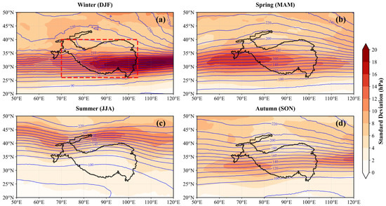
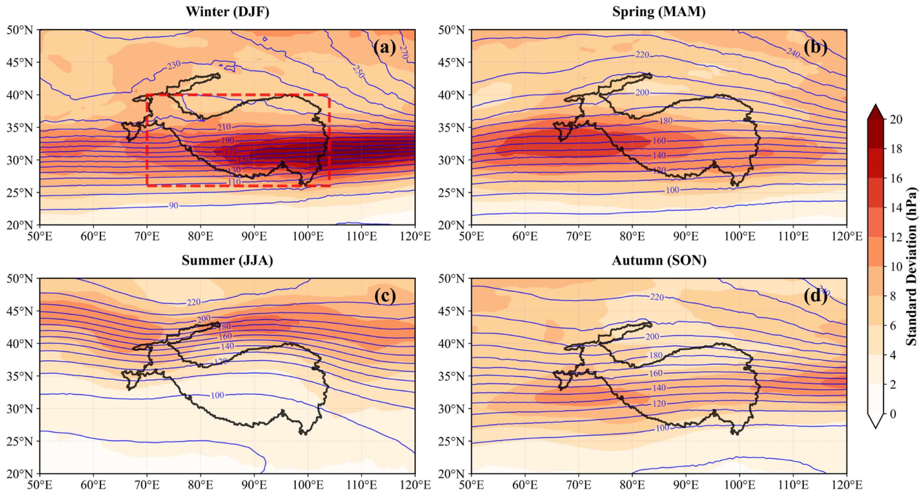
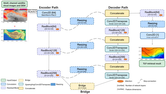
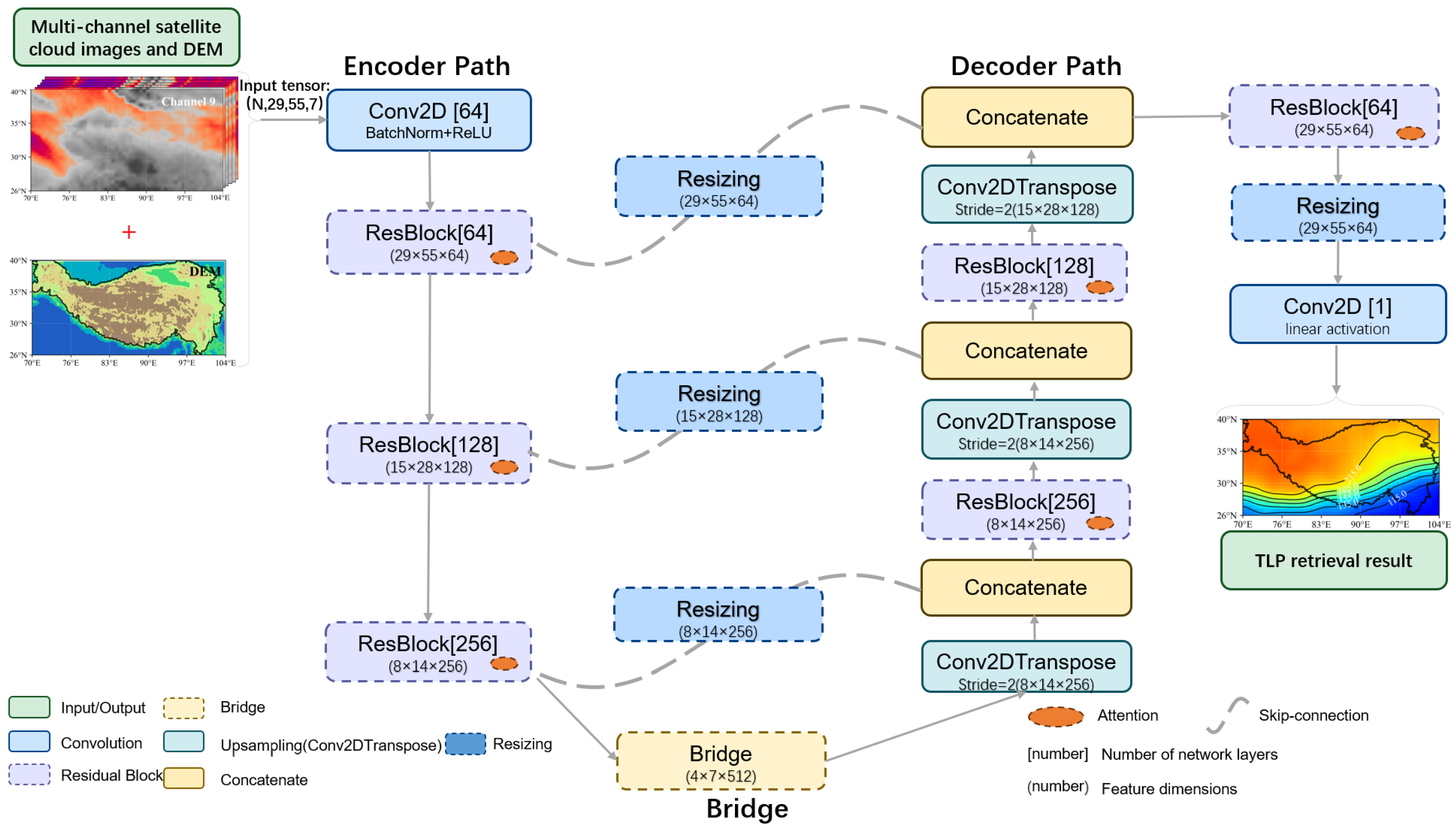
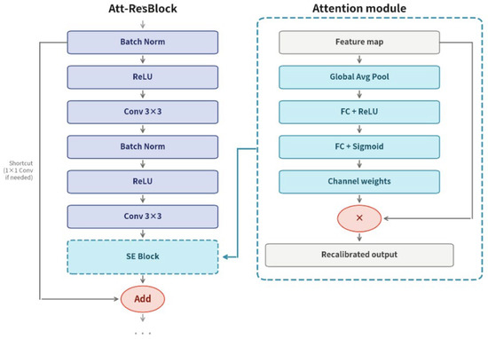
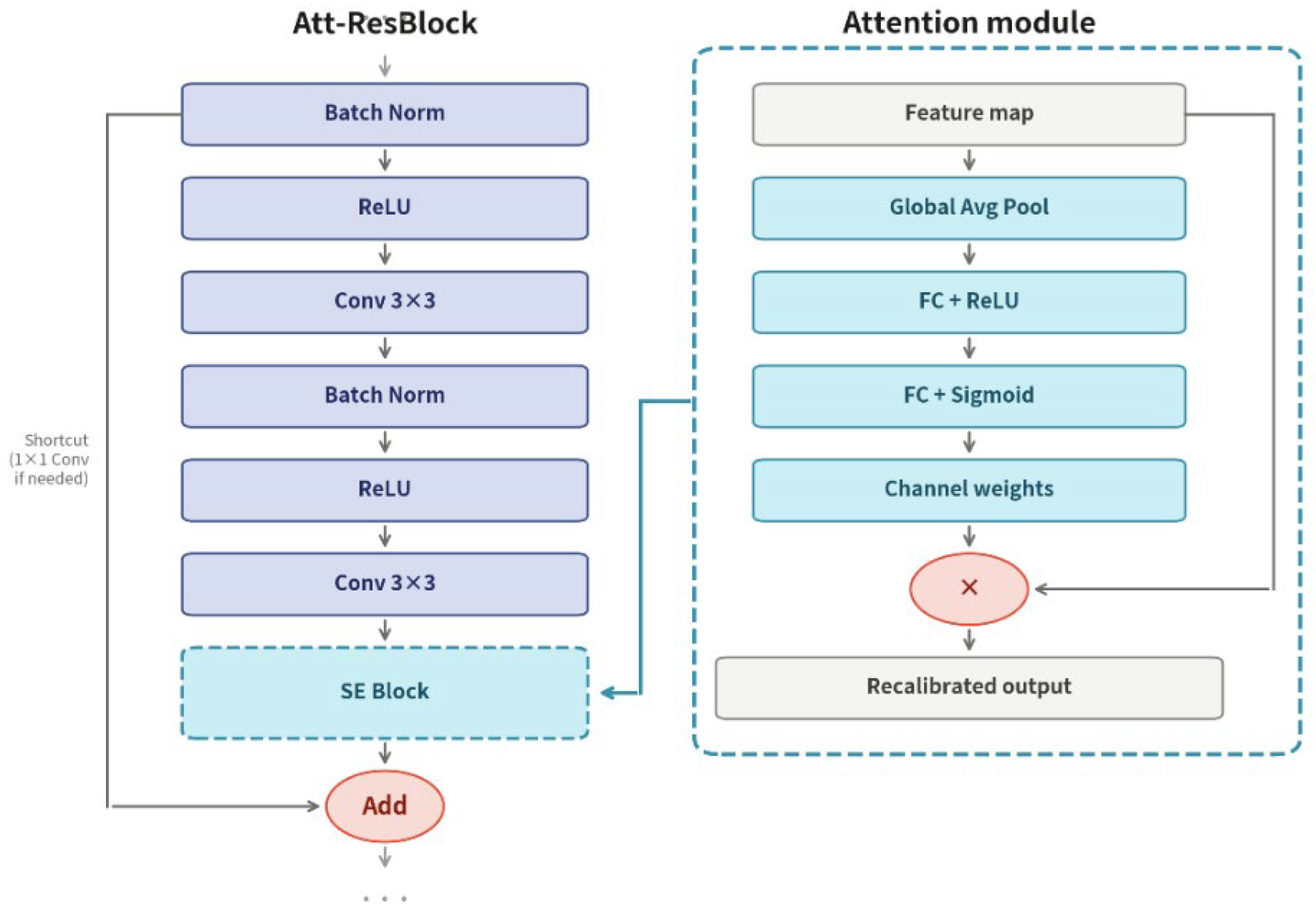
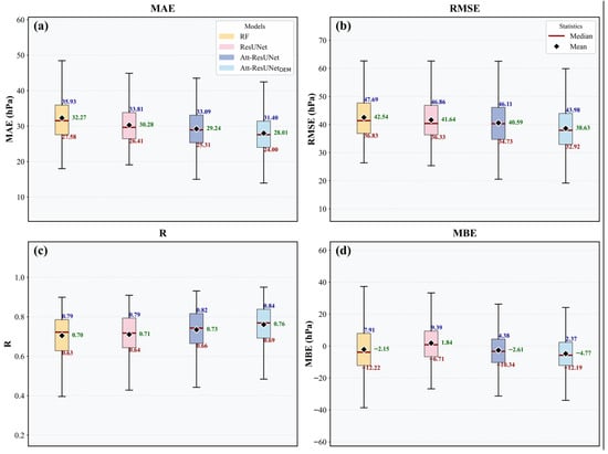
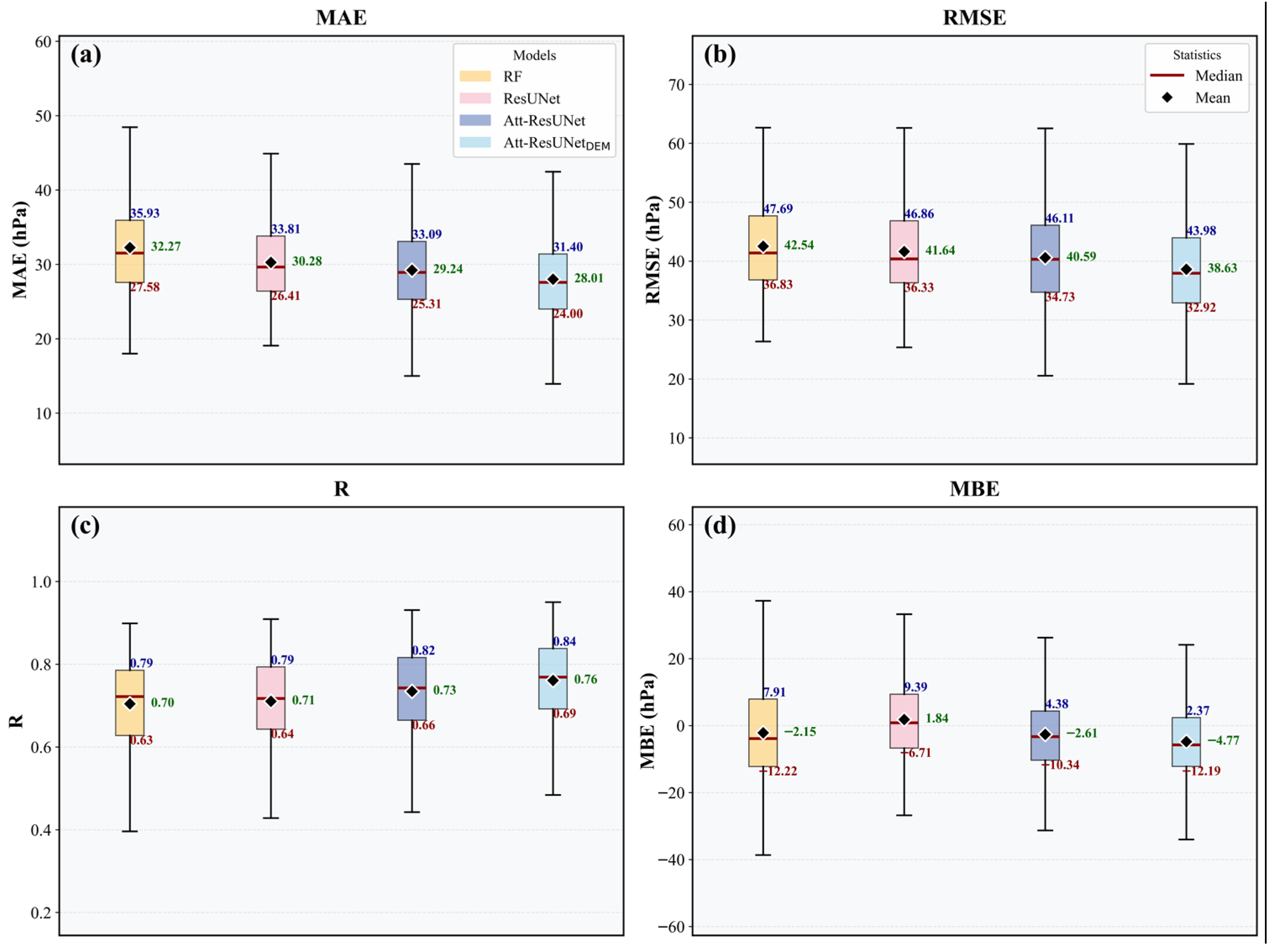
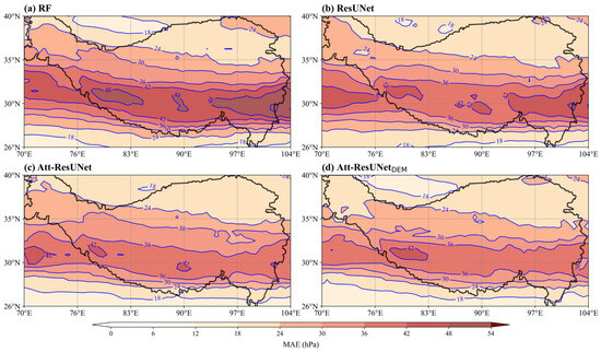
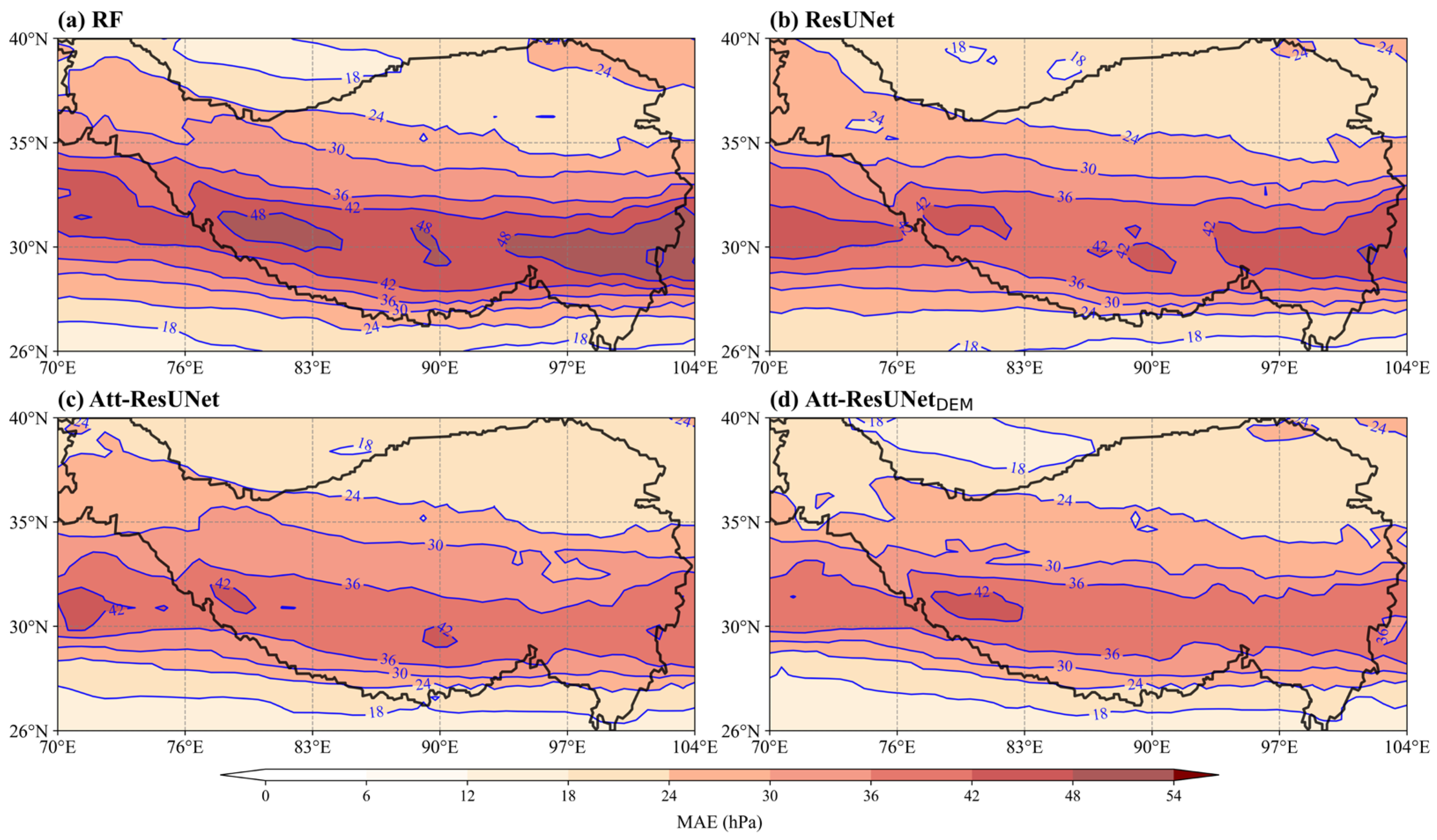
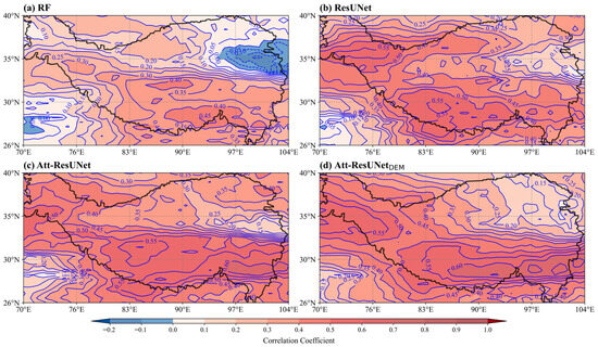
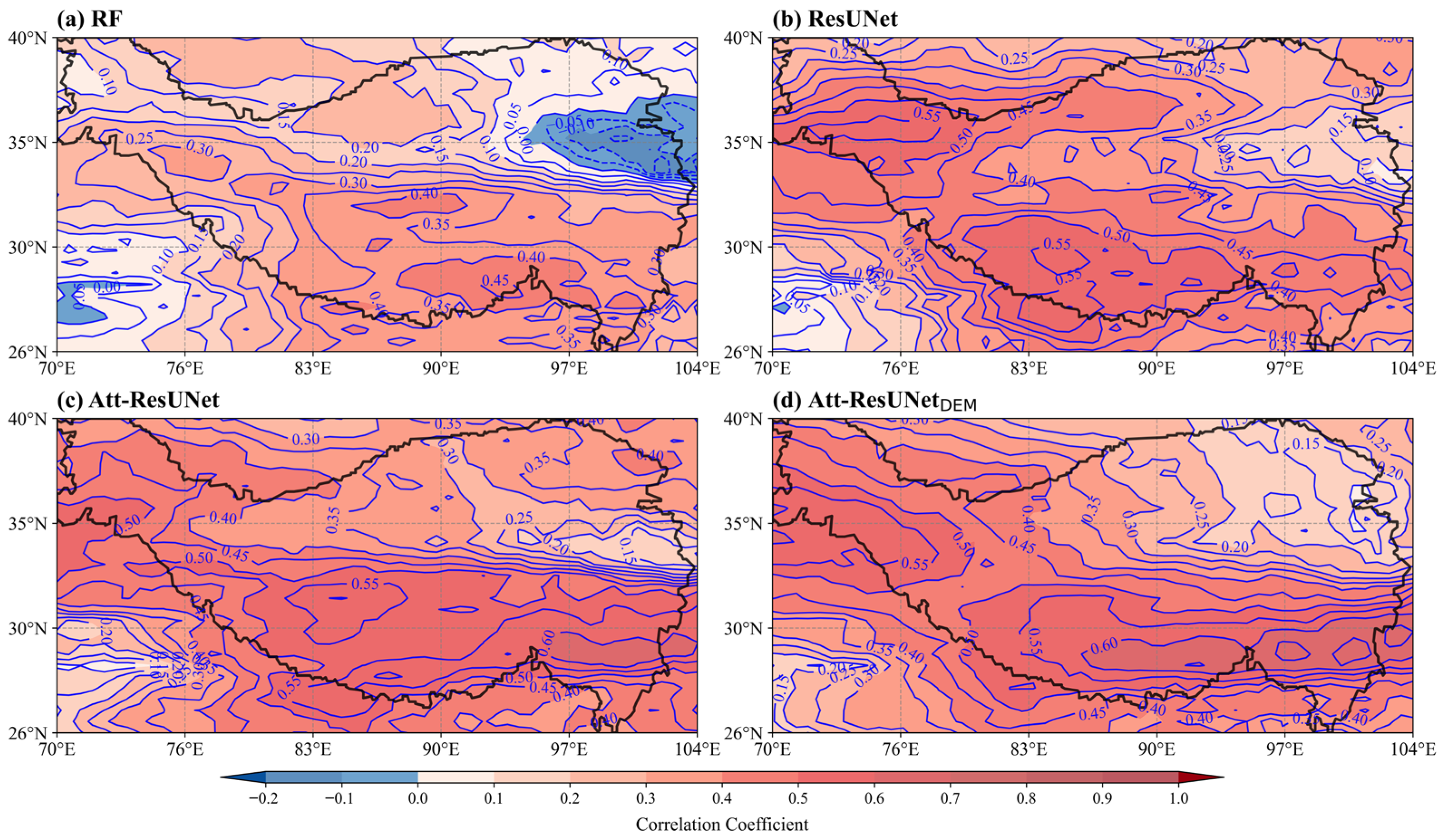
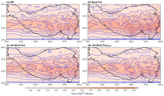
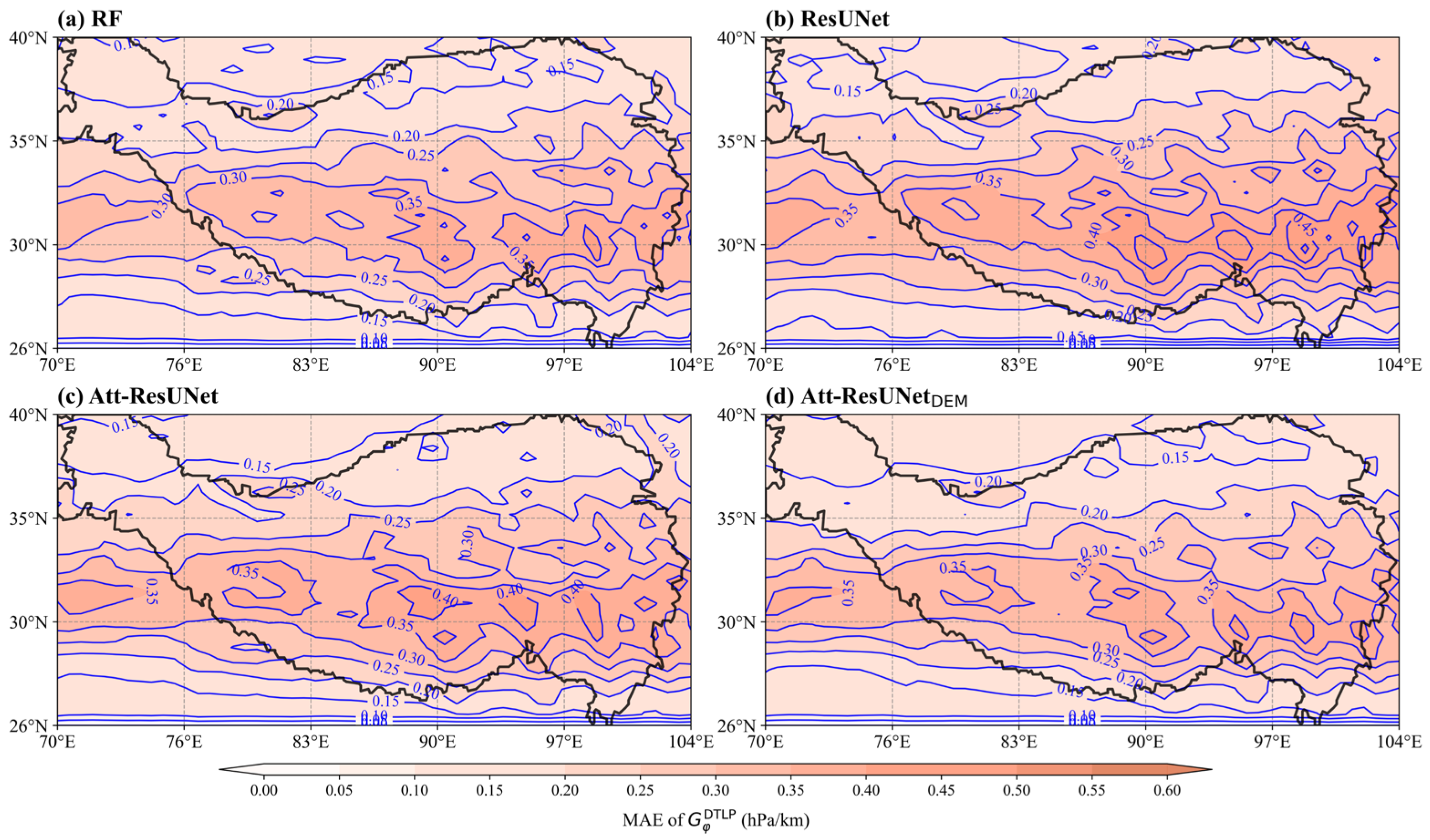
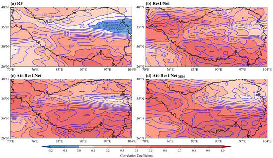
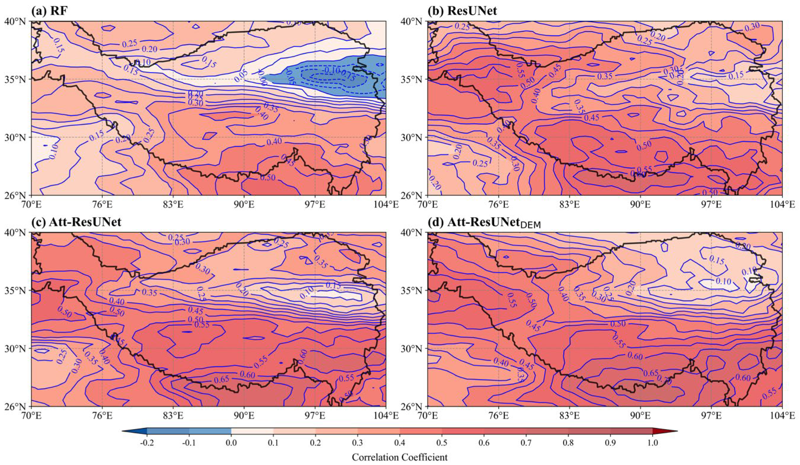
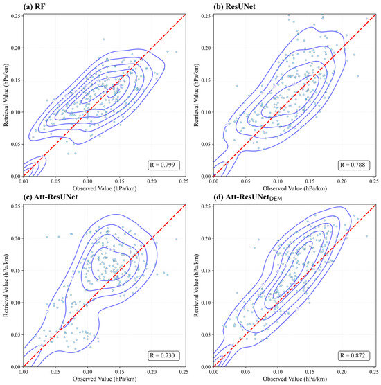
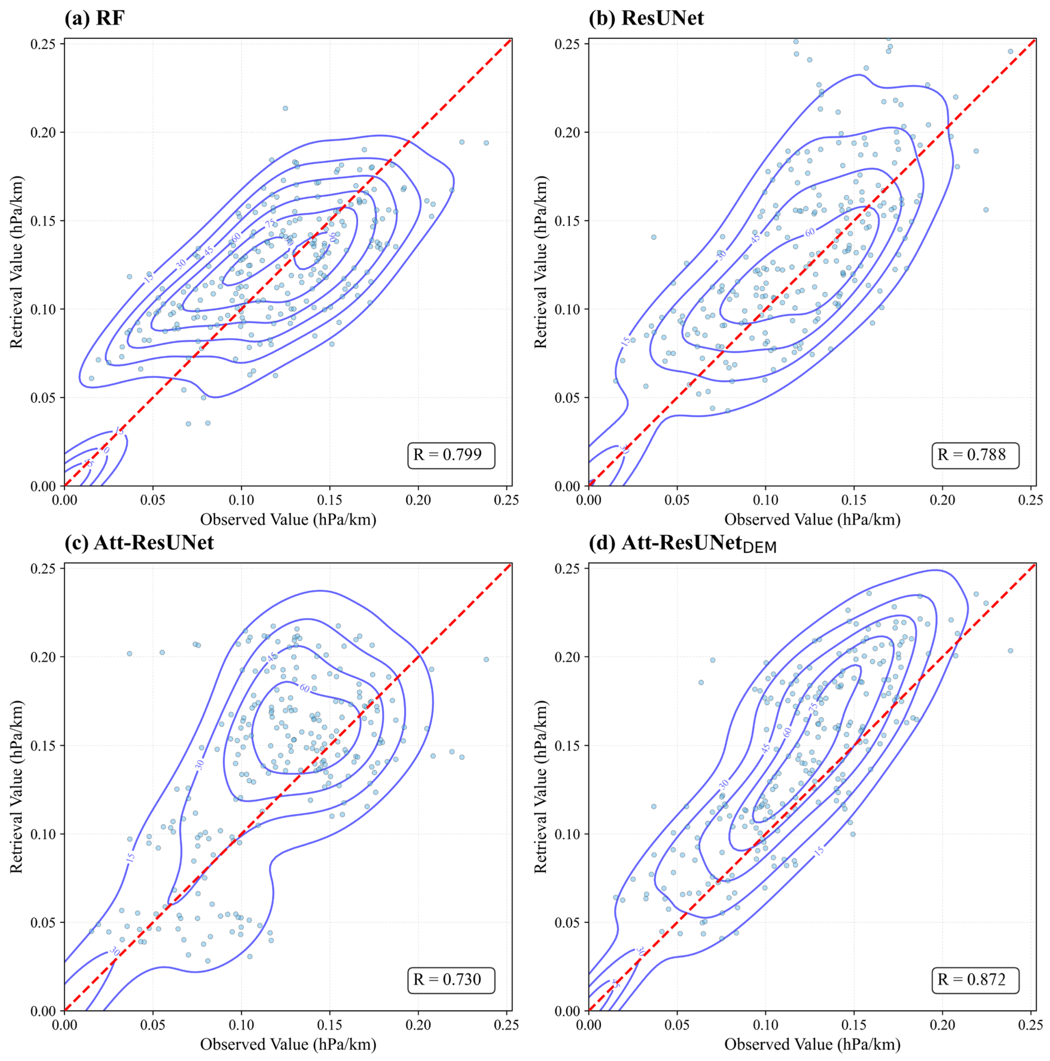
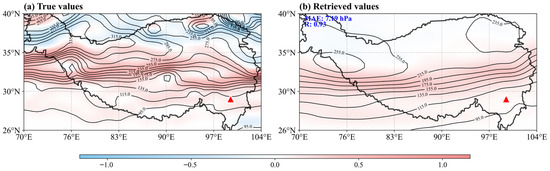
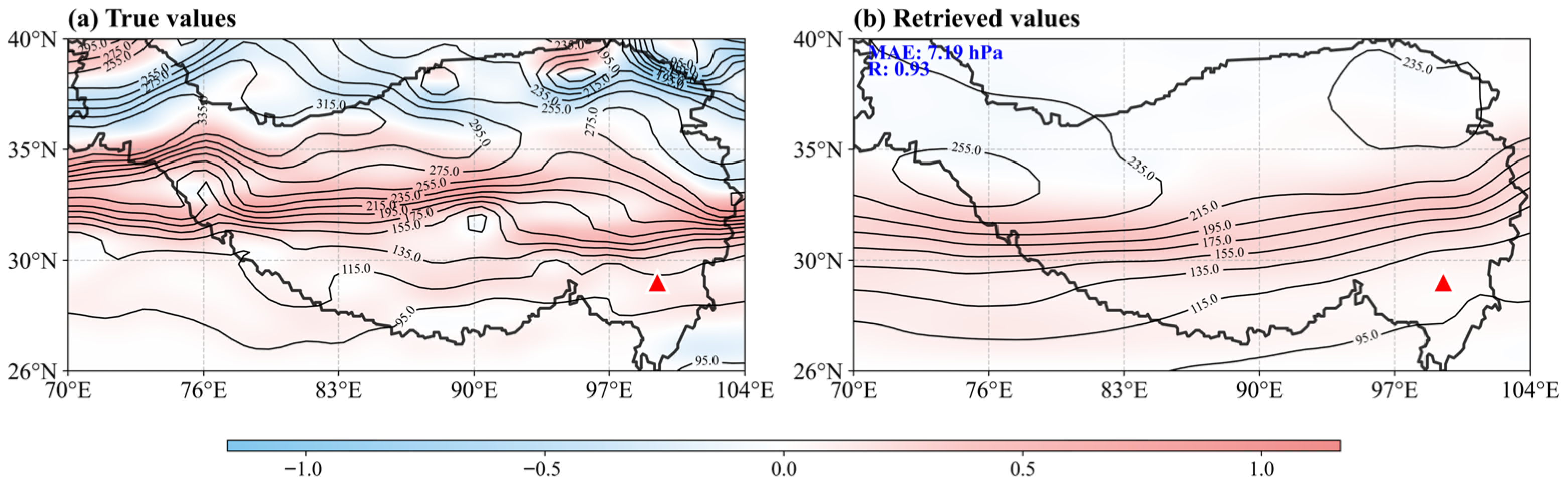
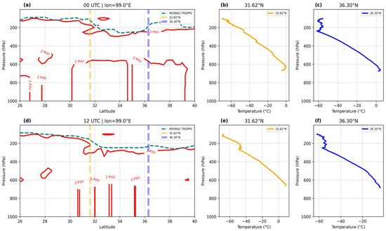
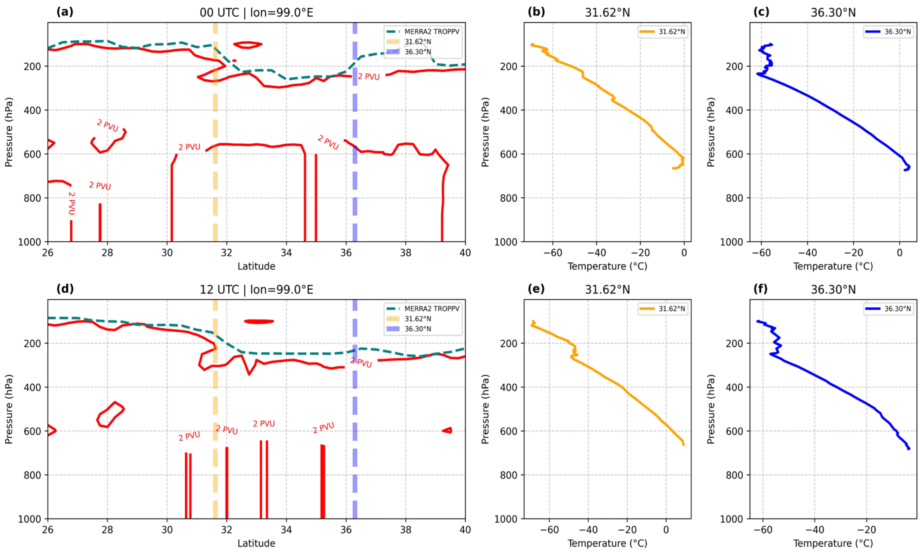
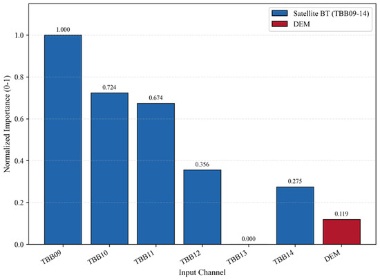
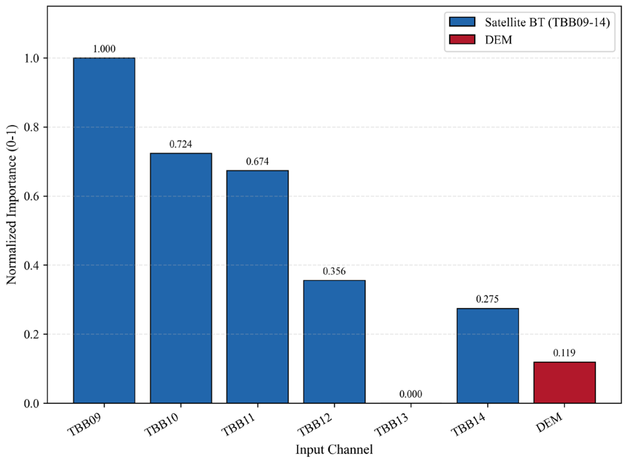

Disclaimer/Publisher’s Note: The statements, opinions and data contained in all publications are solely those of the individual author(s) and contributor(s) and not of MDPI and/or the editor(s). MDPI and/or the editor(s) disclaim responsibility for any injury to people or property resulting from any ideas, methods, instructions or products referred to in the content. |
© 2026 by the authors. Licensee MDPI, Basel, Switzerland. This article is an open access article distributed under the terms and conditions of the Creative Commons Attribution (CC BY) license.