A Multi-Baseline Phase Unwrapping Algorithm Based on Integrated Processing of Intercept Pre-Filtering and Ambiguity Number Vector Determination

Highlights

What are the main findings?

• Extends the ambiguity number linear model and establishes a strict one-to-one mapping between the reference intercepts and ambiguity number combinations.
• Achieves integrated processing of intercept pre-filtering and ambiguity number vector determination.

What are the implications of the main finding?

• Resolves cluster group loss, cluster centerline offset and low computational efficiency of traditional cluster analysis-based algorithms.
• Improves noise robustness and system adaptability for practical InSAR data processing in complex scenes.

Abstract

Multi-baseline phase unwrapping is a critical procedure in interferometric synthetic aperture radar (InSAR) data processing, and cluster analysis (CA)-based algorithms have become an important research direction in this field. However, traditional CA algorithms suffer from cluster group loss, cluster centerline offset under high noise, and time-consuming search, leading to limited unwrapping performance. To address these issues, this article proposes a multi-baseline phase unwrapping algorithm based on the integrated processing of intercept pre-filtering and ambiguity number vector determination, achieving significant performance improvements through four core technical optimisations. First, the linear relationship model of ambiguity numbers is extended to be compatible not only with the traditional one-transmitter, multi-receiver architecture but also with distributed multi-baseline InSAR systems with independent transmit–receive links for each baseline. Second, through verification from both forward and reverse uniqueness perspectives, a strict one-to-one mapping relationship between reference intercepts and ambiguity number combinations is established and validated. Third, a double constraints screening strategy for ambiguity number combinations combining the single-baseline elevation range intersection constraint and the multi-baseline elevation space common intersection constraint is designed. Integrating the effective elevation range of the observation area, this strategy accurately filters out valid ambiguity number combinations with physical rationality, ensuring the reliability of the reference intercept vector. Fourth, an intercept pre-filtering method based on the reference intercept vector is proposed, which unifies actual intercept pre-filtering and ambiguity number vector determination. To verify the performance of the proposed algorithm, a simulation data experiment under varying noise levels and real data experiments are conducted. Results demonstrate that the algorithm can maintain intact cluster structures under complex noise conditions. It achieves a synergistic improvement in unwrapping accuracy and computational efficiency, and thus significantly outperforms comparative algorithms. The proposed algorithm achieves high precision and efficiency for multi-baseline InSAR processing in complex scenarios, with important application value in practical engineering.

1. Introduction

Interferometric synthetic aperture radar (InSAR) is a core technology in the field of microwave remote sensing. It features all-time and all-weather observation capabilities, breaking through the bottleneck of optical remote sensing limited by weather and illumination conditions [1,2]. InSAR plays an irreplaceable role in many fields, including topographic mapping [3], crustal deformation monitoring [4,5], geological hazard early warning [6], urban subsidence analysis [7], and glacier movement tracking [8]. Phase unwrapping is a crucial link in the InSAR data processing workflow [9,10,11,12,13]. The unwrapping accuracy directly determines the reliability of subsequent InSAR results [14,15,16,17]. Single-baseline phase unwrapping algorithms are the foundation of phase unwrapping technology. However, most of these algorithms rely on the phase continuity assumption, which requires the phase difference between adjacent pixels to be less than $\pi$. In areas with terrain mutations, strong noise interference, or low-coherence regions, this assumption is easily violated. This leads to unwrapping errors and even global unwrapping failure, becoming a key bottleneck restricting the application of single-baseline InSAR technology [18]. To break through this limitation, multi-baseline phase unwrapping technology has emerged as the times require [19].

The development of multi-baseline phase unwrapping has undergone a progressive evolution, with research approaches falling mainly into three categories: Chinese Remainder Theorem (CRT)-based methods; cluster analysis (CA)-based methods; and deep learning-based methods. These approaches have undergone continuous optimisation to improve performance, reflecting a shift in research from pure mathematical solution frameworks to physical model-driven optimisation and, more recently, the fusion of traditional algorithms with artificial intelligence technology.

(1) CRT-based Methods: As a classic mathematical solution for multi-baseline phase unwrapping, CRT-based methods focus on solving ambiguity number vectors using the Chinese Remainder Theorem to achieve phase unwrapping. This laid the foundation for the early processing of multi-baseline data. Xu et al. pioneered the analysis of the error characteristics of three typical multi-baseline processing methods: the CRT method, the projection method, and the linear combination method. This provided a critical reference for the improvement of subsequent algorithms [20]. Xia et al. conducted in-depth research on robust CRT-based solution algorithms, overcoming the vulnerability to noise of traditional CRT and establishing a solid basis for the closed-form solution of ambiguity numbers [21,22]. Building on this, Yuan et al. applied the improved, closed-form, robust CRT to multichannel InSAR elevation reconstruction, demonstrating the practical application of CRT-based methods in terrain inversion engineering [23].

(2) CA-based Methods: As research has progressed, CA-based methods have gradually become the main approach to multi-baseline phase unwrapping. These methods have undergone continuous optimisation to improve noise robustness and computational efficiency. Yu et al. first proposed the basic framework of CA-based multi-baseline phase unwrapping. This method groups pixels with the same ambiguity number vector into a single cluster. It achieves this by extracting the intercept term of the multi-baseline phase model. This avoids the low efficiency of pixel-by-pixel calculation [24]. Liu et al. optimised the algorithm in terms of noise robustness, thereby improving its adaptability in the processing of high-noise interferograms [25]. Yuan et al. proposed a closed-form CA-based multi-baseline phase unwrapping and filtering (MBPUF) algorithm that eliminates the need for the time-consuming ambiguity number search step. The algorithm achieves this by providing closed-form solving formulas for ambiguity number vectors, designing a phase filtering strategy and optimising baseline combinations. This results in synergistic improvements in efficiency, noise robustness and elevation reconstruction accuracy [26]. To further suppress noise interference on actual intercepts, Yuan et al. proposed pixel-by-pixel cluster correction (PPCC) and non-core pixel cluster correction (NPCC1, NPCC2) algorithms, and introduced Block-Matching and 3D (BM3D) de-noising technology into intercept pre-filtering [3,27]. Lan et al. further optimised a CA and convex hull-based, fast, large-scale phase unwrapping method for single- and multi-baseline scenarios. The method significantly reduces computational time and memory consumption while ensuring unwrapping accuracy in effective regions by clustering residues in low-quality regions and generating convex hull masks to discard valueless computations [18].

(3) Deep Learning-based Methods: In recent years, methods based on deep learning have revitalised multi-baseline phase unwrapping by learning the feature rules of interferograms and combining them with the logic of traditional algorithms. Zhou et al. proposed the CA-based Network (CANet), an unsupervised deep convolutional neural network specifically designed for CA-based multi-baseline phase unwrapping. It combines the physical model logic of CA with the strong feature extraction ability of deep learning [28]. Liu et al. proposed the Pure Integer Programming Network (PIPNet), which converts the multi-baseline InSAR phase unwrapping problem into a pure integer programming problem. This is then solved using a deep convolutional neural network, which improves the processing efficiency of large-scale interferograms [29]. While deep learning-based methods exhibit excellent feature fitting and large-scale processing capabilities, they rely heavily on high-quality large-scale training datasets and high-performance computing hardware, and their physical interpretability is insufficient, making it difficult to adapt to all complex actual observation scenarios. It is worth noting that traditional multi-baseline phase unwrapping algorithms remain irreplaceable and warrant ongoing optimisation in the era of artificial intelligence. Firmly grounded in physical principles, these algorithms offer strong physical interpretability and do not rely on large-scale training datasets or high-performance hardware. For example, Yan et al. extended the single-baseline phase unwrapping framework to multi-baseline scenarios through a two-stage programming approach (TSPA) [19]; Yue et al. optimised solution accuracy by introducing refined parametric pure integer programming (RPIP) [30]; Li et al. proposed a robust redundant remainder number system (RRNS) for high-precision terrain elevation inversion [31].

This paper proposes a multi-baseline phase unwrapping algorithm based on the integrated processing of intercept pre-filtering and ambiguity number vector determination, aiming to address the problems of cluster group loss, cluster centerline offset and inefficient search procedures of traditional CA algorithms. The overall performance of the algorithm is improved through four core optimisations. First, the linear relationship model of ambiguity numbers is expanded and reconstructed to adapt to the distributed InSAR architecture with independent transmit–receive links, while being compatible with the traditional one-transmitter, multi-receiver architecture. This breaks through the application scenario limitations of the original model, and the corresponding extended intercept calculation model is derived synchronously. Second, based on the extended linear model, a strict one-to-one mapping relationship between reference intercepts and ambiguity number combinations is established and verified, laying a solid theoretical foundation for their subsequent direct mutual derivation. Third, a double constraints screening strategy for ambiguity number combinations is designed. Combined with the effective elevation range of the observation area, the valid integer interval of single-baseline ambiguity numbers is first determined through the single-baseline elevation range intersection constraint. Then the multi-baseline elevation space common intersection constraint is used to verify whether there is a non-empty intersection between the elevation spaces corresponding to the ambiguity number combination. In this way, the valid ambiguity number combinations with physical rationality are accurately filtered out, which ensures the reliability of the reference intercept vector constructed on this basis. Finally, an intercept pre-filtering method based on the reference intercept vector is proposed, which realises the integrated processing of actual intercept pre-filtering and ambiguity number vector determination. By matching the actual intercept with the reference intercept vector and relying on the above-mentioned strict one-to-one mapping relationship, the corresponding ambiguity number combination can be directly derived. This integrated processing mode directly eliminates the time-consuming search steps in traditional algorithms, laying a foundation for the synergistic improvement of unwrapping accuracy and computational efficiency.

The rest of this paper is organised as follows. Section 2 analyses the core principles of the traditional CA algorithm and existing intercept pre-filtering algorithms, and elaborates on their application limitations. Section 3 details the principles and specific implementation steps of the proposed algorithm. Section 4 verifies the performance of the proposed algorithm through simulation and real data experiments. Section 5 summarises the overall research work of this paper and prospects future research directions.

2. Analysis of the CA Algorithm and Intercept Pre-Filtering

In this section, we derive the core principles of the traditional CA algorithm for the one-transmitter, multi-receiver multi-baseline InSAR architecture, and analyse its inherent defects as well as existing intercept pre-filtering algorithms, laying a theoretical foundation for designing the improved algorithm thereafter.

For any pixel in the observation scene, the height h satisfies the following relationship:

$$h={\displaystyle \frac{H_i({\phi }_i+2k_i\pi )}{2\pi }}$$

(1)

Here, $i=1,2,...,N$, where N is the number of baselines. ${\phi }_i$, $H_i$, and $k_i$ represent the flattened interferometric phase, ambiguity height, and ambiguity number for Baseline i, respectively. The definition of ambiguity height $H_i$ is

$$H_i={\displaystyle \frac{\lambda Rsin\theta }{B_i}}$$

(2)

where $B_i$ is the vertical effective baseline for Baseline i. R and $\theta$ represent the slant range and look angle of the transmitting satellite, respectively. $\lambda$ denotes the wavelength of the signal. By combining Equations (1) and (2) with Baseline 1 as the reference baseline, the linear model for ambiguity numbers can be derived:

$$k_1={\displaystyle \frac{B_1}{B_j}}{k}_j+{\displaystyle \frac{B_1{\phi }_j-B_j{\phi }_1}{2\pi B_j}}$$

(3)

Here, $j=2,...,N$. ${\phi }_j$, $B_j$, and $k_j$ represent the flattened interferometric phase, vertical effective baseline, and ambiguity number for Baseline j, respectively.

In this model, the intercept term is

$$Intercept={\displaystyle \frac{B_1{\phi }_j-B_j{\phi }_1}{2\pi B_j}}$$

(4)

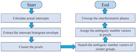
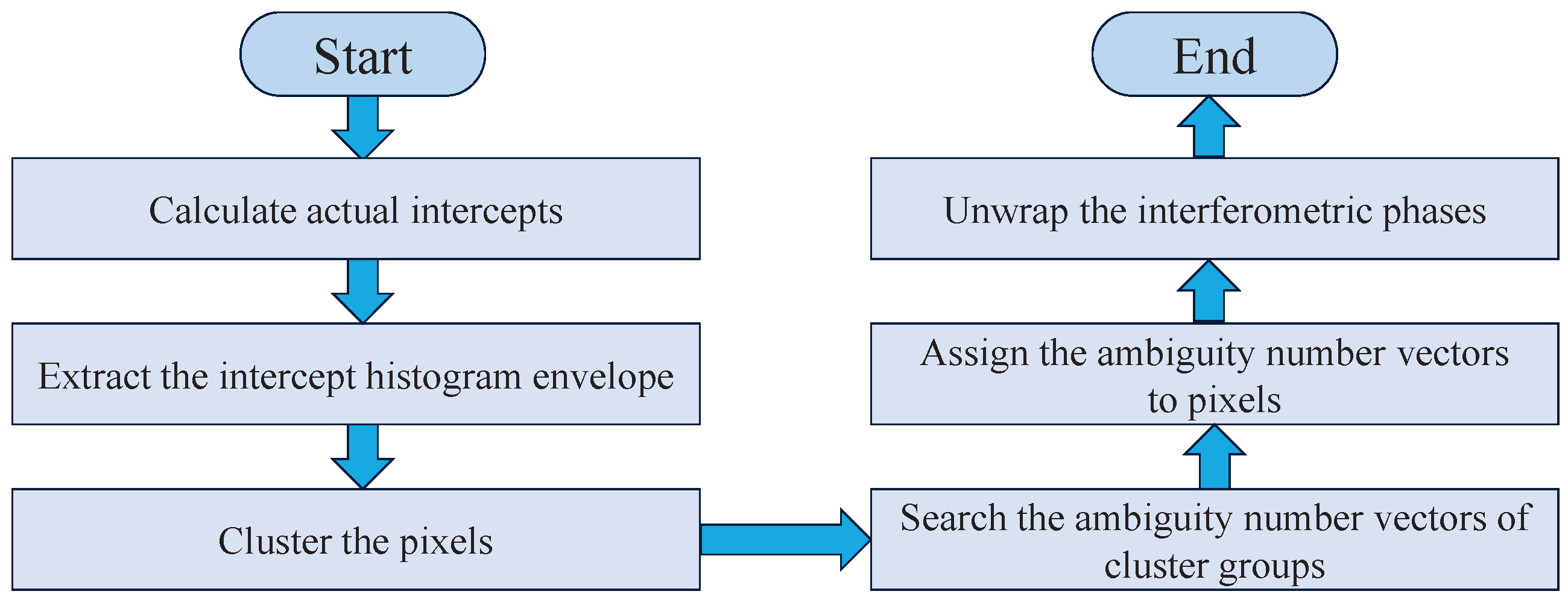
The detailed steps of the CA algorithm are described below with reference to Figure 1:

Figure 1. Flowchart of the CA algorithm.

① Calculate the actual intercept of each pixel: Solve for the actual intercept corresponding to each pixel in accordance with (4).

② Conduct intercept histogram statistics and extract the envelope: Divide the intercept axis into equidistant unit intervals, count the number of pixels in each interval via the histogram method, and extract the envelope curve of the histogram.

③ Perform pixel clustering and grouping: Identify the troughs of the envelope curve to separate individual peaks (one peak corresponding to one cluster group), and assign pixels to the corresponding cluster groups based on their affiliated peaks.

④ Solve for ambiguity number vectors: Take the abscissa of each peak as the cluster centerline, substitute it into (4), and select the integer point closest to the centerline within the ambiguity number search range as the ambiguity number vector of the corresponding cluster group.

⑤ Assign ambiguity number vectors to pixels: Uniformly assign the ambiguity number vector of each cluster group to all pixels within the group.

⑥ Implement phase unwrapping: Perform ambiguity elimination on the interferometric phase based on the solved ambiguity number vector to complete the phase unwrapping process.

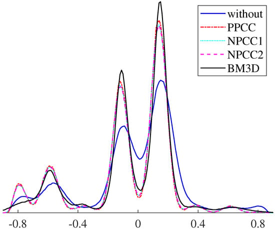
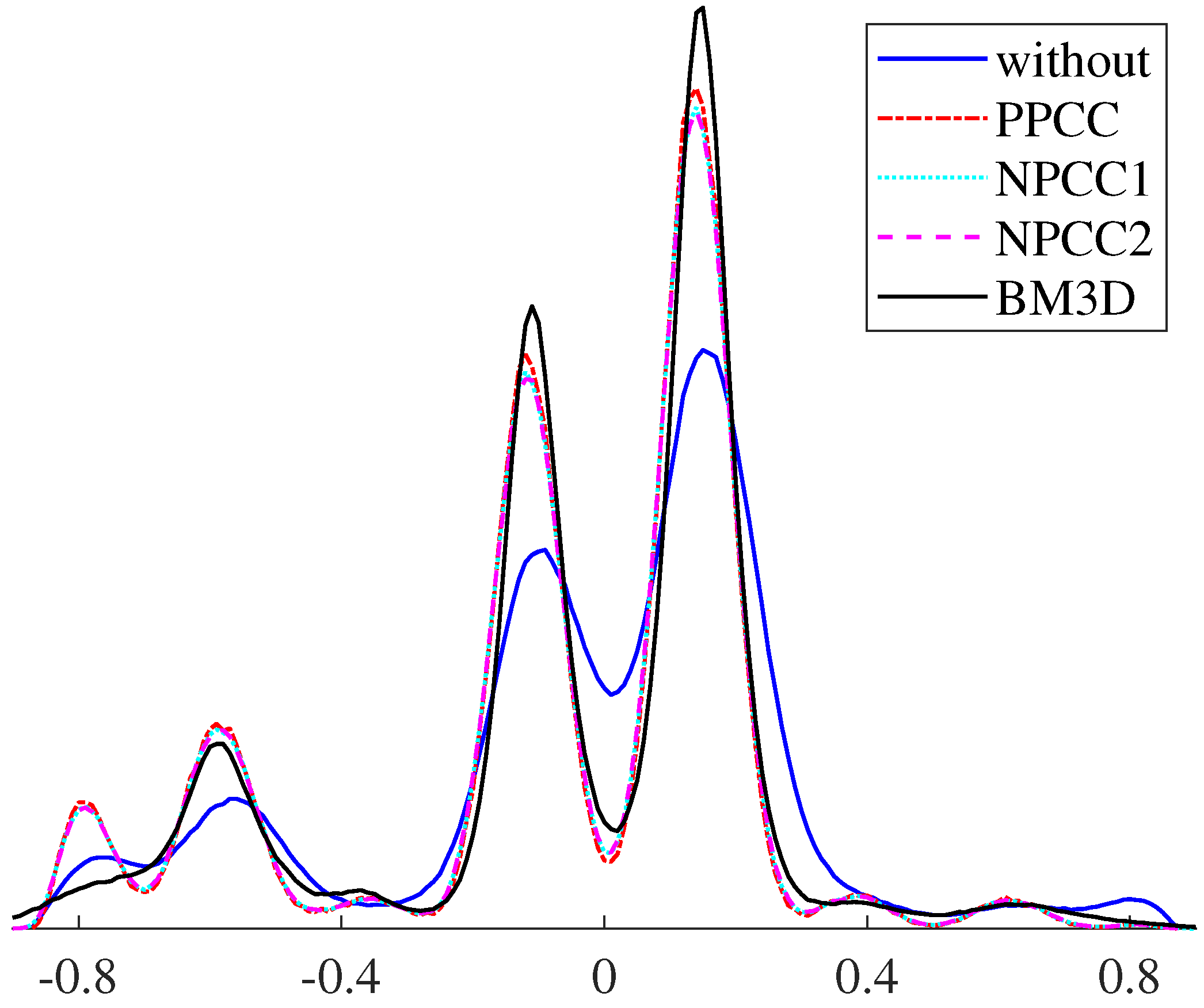
The core principle of the CA algorithm is to group all pixels based on the intercept term and solve for the ambiguity number vector uniformly within each cluster group, which avoids the low-efficiency problem caused by traditional pixel-by-pixel calculation. In practice, the CA algorithm needs to locate cluster centerlines by searching for peaks in the intercept statistical graph. The presence of phase noise can severely distort the statistical distribution characteristics of intercepts, as qualitatively illustrated by the solid blue line in Figure 2, leading to a significant degradation in the algorithm’s performance.

Figure 2. Qualitative comparison of intercept distributions between the without pre-filtering and four existing intercept pre-filtering algorithms under high-noise condition. The horizontal axis represents the intercept value.

To address this key issue, intercept pre-filtering has emerged as an effective solution, and various intercept pre-filtering algorithms have been proposed in existing studies. Ref. [27] designed the PPCC algorithm, as well as two types of non-core pixel cluster correction algorithms (NPCC1 and NPCC2). Ref. [3] applied the BM3D filtering technology to suppress intercept noise. However, as can be seen from the red, cyan, purple and black lines in Figure 2, these algorithms only optimise the statistical distribution of intercepts to facilitate subsequent cluster centerline searches. They can mitigate, but not fully resolve, core problems such as cluster group loss and cluster centerline offset that may occur during the clustering process. Moreover, these algorithms cannot avoid the subsequent ambiguity number search, which still takes substantial computational time. Meanwhile, their unresolved problems can be propagated to the subsequent search step, resulting in errors in ambiguity number vector searching.

3. Proposed Algorithm

To address the core issues of cluster group loss, cluster centerline offset, and inefficient search procedures of traditional CA algorithms discussed in Section 2, this section proposes the multi-baseline phase unwrapping algorithm based on integrated processing of intercept pre-filtering and ambiguity number vector determination, with its performance significantly improved through four key technical optimisations. The specific improvements are as follows: (1) The linear relationship of ambiguity numbers is expanded and reconstructed. (2) A strict one-to-one mapping relationship between reference intercepts and ambiguity number combinations is established and verified from both forward and reverse uniqueness perspectives. (3) A double constraints screening strategy for ambiguity number combinations is designed to filter out valid combinations with physical rationality. (4) An actual intercept pre-filtering method is developed, which takes reference intercepts as the core benchmark to realise the integrated processing of actual intercept pre-filtering and ambiguity number vector determination. The pseudocode of the proposed algorithm is provided at the end of this section.

3.1. Extension of the Ambiguity Number Linear Relationship Model

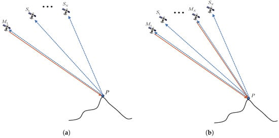
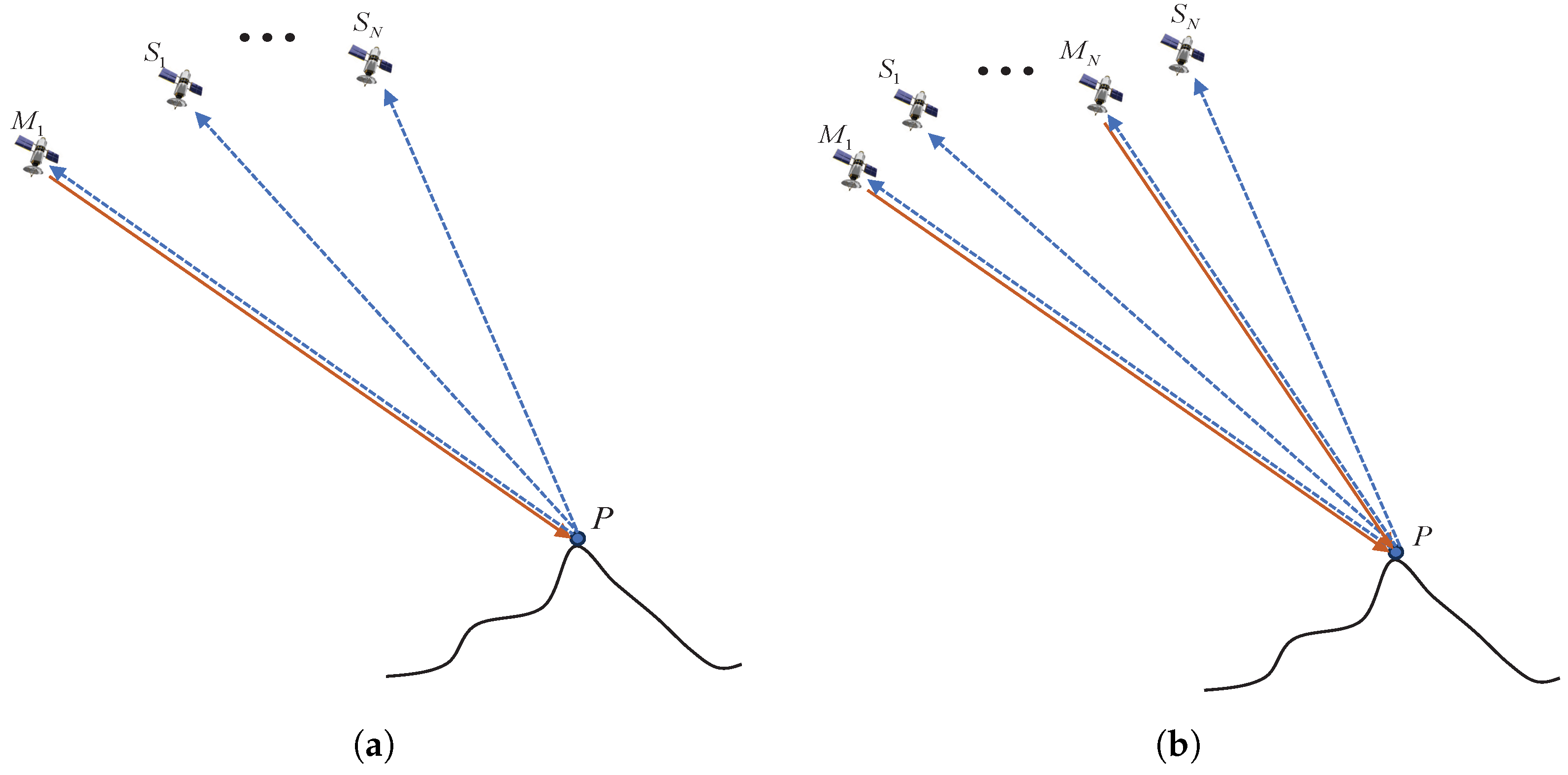
The ambiguity number linear relationship model derived in Section 2 is applicable to a multi-baseline InSAR system with a one-transmitter, multi-receiver architecture, as illustrated in Figure 3a. Such a system employs one transmitter and multiple receivers, with all baselines sharing the same transmit link. Consequently, the transmitter slant range and the corresponding radar look angle for different baselines can be considered as global constants. However, in a distributed multi-baseline InSAR architecture illustrated in Figure 3b, each baseline corresponds to a separate transmit–receive link. There are obvious differences in the spatial geometry between different baselines, which is reflected in the fact that the transmitter slant ranges and radar look angles are no longer identical across baselines. Under these conditions, the fundamental assumptions of the one-transmitter, multi-receiver architecture are invalidated, rendering the model inapplicable.

Figure 3. Architectures of multi-baseline InSAR systems. (a) One-transmitter, multi-receiver multi-baseline InSAR architecture; (b) multi-baseline InSAR architecture with independent transmit–receive links for each baseline. Herein, $M_1$, …, $M_N$ represent transmit satellites and $S_1$, …, $S_N$ represent receive satellites, solid lines denote transmit links and dashed lines denote receive links. In (a), $M_1$ transmits signals, and $M_1$, $S_1$, …, $S_N$ receive the echo signals almost simultaneously, meaning that the N baselines constructed (consisting of $M_1$ combined with $S_1$, …, $S_N$ respectively) share the same transmit link. In (b), $M_1$ transmits signals, while $M_1$ and $S_1$ receive the echo signals almost simultaneously; by analogy, $M_N$ transmits signals, while $M_N$ and $S_N$ receive the echo signals almost simultaneously, which means that the N baselines constructed (consisting of the pairwise combinations of $M_1$ and $S_1$, …, $M_N$ and $S_N$) are all equipped with independent transmit–receive links. The schematic diagram of this architecture in (b) can either characterise multiple groups of satellites observing the same area or a single group of satellites conducting multiple observations of the same area.

To address this issue, this subsection expands and reconstructs the ambiguity number linear relationship model to be compatible with both the traditional one-transmitter, multi-receiver architecture and scenarios with independent transmit–receive links. The core differences between the original model and the extended model are compared in the Table 1, followed by the introduction of the extended model based on this comparison.

Table 1. Comparison of the original and extended models.

	Original Model	Extended Model
Applicable architecture	One-transmitter multi-receiver	Independent transmit–receive links
Core geometric parameters	Unified R, $\theta$ for all baselines	Baseline-specific $R_i$, ${\theta }_i$

First, an extended, generalised definition of ambiguity height is introduced, whereby the ambiguity height of each independent baseline is determined by its geometric parameters alone. The expression is given as follows:

$$H_i={\displaystyle \frac{\lambda R_{i}sin{\theta }_i}{B_i}}$$

(5)

where $R_i$ and ${\theta }_i$ represent the slant range and look angle of the transmitting satellite for Baseline i, respectively.

Based on (1) and (5), with Baseline 1 as the reference baseline, the extended model for the linear relationship between ambiguity numbers under independent transmit–receive links is derived:

$$k_1={\displaystyle \frac{B_1{R}_{j}sin{\theta }_j}{B_j{R}_{1}sin{\theta }_1}}{k}_j+{\displaystyle \frac{B_1{\phi }_j{R}_{j}sin{\theta }_j-B_j{\phi }_1{R}_{1}sin{\theta }_1}{2\pi B_j{R}_{1}sin{\theta }_1}}$$

(6)

where $R_1$ and ${\theta }_1$ represent the slant range and look angle of the transmitting satellite for Baseline 1, respectively. $R_j$ and ${\theta }_j$ represent the slant range and look angle of the transmitting satellite for Baseline j ($j=2,...,N$), respectively.

At the same time, the extended intercept model can be obtained:

$$Inter={\displaystyle \frac{B_1{\phi }_j{R}_{j}sin{\theta }_j-B_j{\phi }_1{R}_{1}sin{\theta }_1}{2\pi B_j{R}_{1}sin{\theta }_1}}$$

(7)

This extended model can adapt to geometric conditions where the transmitter slant range and radar look angle vary across different baselines.

According to (6), the linear relationship between the intercept and ambiguity number is obtained:

$$Inter=k_1-{\alpha }_j{k}_j$$

(8)

where ${\alpha }_j$ is a proportionality coefficient:

$${\alpha }_j={\displaystyle \frac{B_1{R}_{j}sin{\theta }_j}{B_j{R}_{1}sin{\theta }_1}}={\displaystyle \frac{H_j}{H_1}}$$

(9)

where $H_1$ and $H_j$ are the ambiguity heights of Baseline 1 and Baseline j, respectively. ${\alpha }_j$ is jointly determined by the geometric parameters of InSAR systems, including the vertical effective baselines, slant ranges, and radar look angles.

A comparison of (3) and (8) reveals that the two models employ different proportional coefficients in their respective linear relationships. When the differences between $R_1$ and $R_j$ and between ${\theta }_1$ and ${\theta }_j$ are small, the results of the two models are similar. However, when these geometric parameters differ considerably, the extended model’s advantage becomes significant, as it effectively avoids large deviations in the calculated intercept.

For the traditional one-transmitter, multi-receiver architecture, $R_1$ = $R_j$ and ${\theta }_1$ = ${\theta }_j$ for all j, and substituting these into (6) and (7) directly simplifies them to (3) and (4). The proposed model can be flexibly adapted to different InSAR architectures by substituting corresponding geometric parameters. In practical systems, millimetre-level baseline errors, look angle errors in the range of 0.001° to 0.01°, and metre-level slant range errors are inevitably present. For (7), the intercept is obtained by normalising the geometric-phase coupling difference term in the numerator with the geometric parameters in the denominator. Benefiting from the hundreds-of-kilometre-scale slant range contained in the denominator, an extremely large numerical magnitude is yielded, which imposes an inherent normalisation suppression effect on the absolute errors of all geometric parameters. As a result, the impacts of such errors on intercept calculation are negligible, demonstrating that the proposed model possesses favourable robustness against actual geometric parameter errors.

3.2. Construction of the Strict One-to-One Mapping Relationship Between Reference Intercepts and Ambiguity Number Combinations

According to (9), ${\alpha }_j$ in (8) is a constant, and thus the reference intercept is solely determined by the linear combination of $k_1$ and $k_j$.

Below, the strict one-to-one mapping relationship between reference intercepts and ambiguity number combinations is demonstrated and verified from two aspects: forward uniqueness and reverse uniqueness.

• Forward uniqueness: one valid ambiguity number combination corresponds to a unique reference intercept.

For a valid ambiguity number combination $(k_1,k_j)$, $k_1$ and $k_j$ are definite integers. Meanwhile, ${\alpha }_j$ is a constant of the system. According to the linear operation rule of (8), the linear combination of integers and a constant yields a unique result. Therefore, one ambiguity number combination can only be calculated to obtain one reference intercept, with no one-to-many correspondence.

• Reverse uniqueness: one valid reference intercept corresponds to a unique ambiguity number combination.

Reverse uniqueness means that, under actual observation conditions, a reference intercept corresponds uniquely to an ambiguity number combination.

A proof by contradiction is adopted here. Assume that there exist two distinct ambiguity number combinations $(k_1^{\left(1\right)},k_j^{\left(1\right)})$ and $(k_1^{\left(2\right)},k_j^{\left(2\right)})$ that correspond to the same reference intercept $Inte{r}^0$. Then the following relationship can be obtained:

$$k_1^{\left(1\right)}-{\alpha }_j{k}_j^{\left(1\right)}=k_1^{\left(2\right)}-{\alpha }_j{k}_j^{\left(2\right)}$$

(10)

Rearranging (10) yields:

$$\Delta k_1={\alpha }_j\Delta k_j$$

(11)

where $\Delta k_1=k_1^{\left(1\right)}-k_1^{\left(2\right)}$ and $\Delta k_j=k_j^{\left(1\right)}-k_j^{\left(2\right)}$. Since the two sets of combinations are different, $\Delta k_1$ and $\Delta k_j$ are non-zero integers. Substituting ${\alpha }_j=H_j/H_1$ into (11) gives

$$\Delta k_1{H}_1=\Delta k_j{H}_j$$

(12)

From (12), it can be concluded that different ambiguity number combinations can correspond to the same reference intercept only if there exist non-zero integers $\Delta k_1$ and $\Delta k_j$ satisfying $\Delta h=\Delta k_1{H}_1=\Delta k_j{H}_j$, where $\Delta h$ represents the elevation difference associated with the two ambiguity number combinations. In other words, $\Delta h$ must be a common multiple of $H_1$ and $H_j$.

Based on the above condition, the intercept non-repeating elevation is defined as follows. The intercept non-repeating elevation $H_{LCM}$ denotes the minimum elevation difference that causes intercept repetition. It is defined as the smallest elevation satisfying $\Delta h=\Delta k_1{H}_1=\Delta k_j{H}_j$ and is equivalent to the least common multiple (LCM) of $H_1$ and $H_j$, expressed as

$$H_{LCM}={\displaystyle \frac{H_1{H}_j}{\gcd (H_1,H_j)}}$$

(13)

where $\gcd (H_1,H_j)$ denotes the greatest common divisor of $H_1$ and $H_j$. Physically, the intercept non-repeating elevation represents the critical elevation threshold for avoiding reference intercept repetition. Only when the terrain elevation difference exceeds this threshold can different ambiguity number combinations produce the same reference intercept.

In practical engineering scenarios, ambiguity heights $H_1$ and $H_j$ are derived from precise geometric parameters, including radar wavelength, slant range, incidence angle, and vertical effective baseline, and thus typically take multi-decimal values. As a result, the greatest common divisor $\gcd (H_1,H_j)$ is generally extremely small, yielding a least common multiple $H_{LCM}$ that can reach tens of thousands of metres or even higher. Since real-world terrain elevation variations are usually only hundreds to thousands of metres, which is far smaller than $H_{LCM}$, no non-zero integers $\Delta k_1$ and $\Delta k_j$ exist that satisfy $\Delta k_1{H}_1=\Delta k_j{H}_j$. In rare extreme cases where $H_{LCM}$ might be insufficiently large, retaining more decimal places in the calculation of ambiguity heights can ensure $H_{LCM}$ remains sufficiently large. Therefore, the reverse uniqueness property is valid under realistic InSAR system configurations and observation conditions.

3.3. Double Constraints Screening for Ambiguity Number Combinations

As derived in Section 3.2, there is a strict one-to-one mapping relationship between reference intercepts and ambiguity number combinations. Thus, the calculation of a reference intercept can be accomplished simply by substituting the corresponding ambiguity number combination $(k_1,k_j)$ into (8). This unique one-to-one mapping relationship also establishes the fundamental prerequisite for the reference intercept calculation method outlined in Section 3.2: the input ambiguity number combinations $(k_1,k_j)$ must have a valid physical interpretation. If the values of an ambiguity number combination $(k_1,k_j)$ deviate from the constraints of actual elevation conditions, a numerical intercept result can still be derived by (8), but such a result will lack the support of actual elevation and thus become an invalid intercept with no physical meaning. Such invalid intercepts may fail to provide a reliable theoretical benchmark for subsequent intercept pre-filtering. They can also lead to an unnecessary increase in computational load and distortion in intercept pre-filtering. This directly reduces the overall accuracy of multi-baseline phase unwrapping.

To address this issue, this subsection proposes a double constraints screening method for ambiguity number combinations. This method adopts a hierarchical screening mechanism. The single-baseline elevation range intersection constraint first performs preliminary dimensionality reduction on individual ambiguity numbers, and the multi-baseline elevation space common intersection constraint then verifies the rationality of ambiguity number combinations, ensuring that the screened ambiguity number combinations have strict physical rationality.

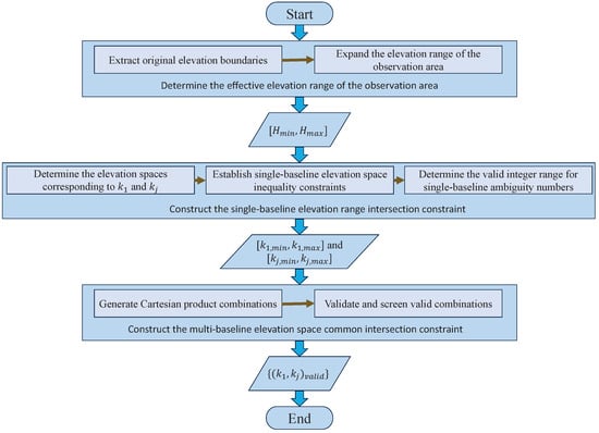
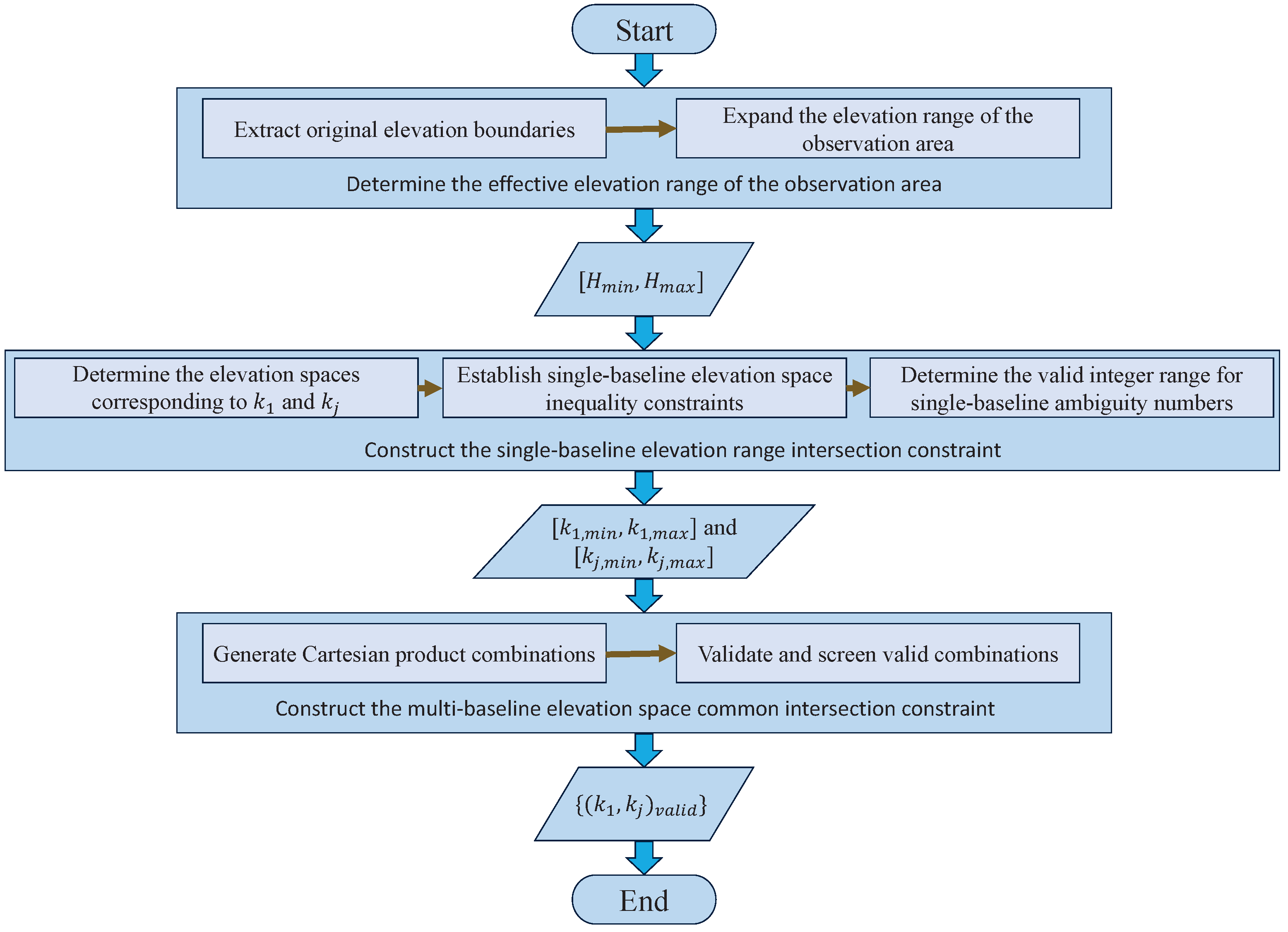
The double constraints screening for ambiguity number combinations is explained in detail with Figure 4 below.

Figure 4. Flowchart of double constraints screening for ambiguity number combinations.

• Determination of the effective elevation range of the observation area.

Double constraints screening for ambiguity number combinations requires the effective elevation range of the observation area to be used as a quantitative benchmark. Only the extreme values at the elevation boundaries need to be extracted to meet the constraint determination requirements. The specific steps are as follows:

(1) Extraction of original elevation boundaries: The original minimum and maximum elevations are extracted from a low-precision external reference elevation database according to the geographic latitude and longitude extent of the observed area. Notably, only the extreme maximum and minimum elevation values of the observed area are adopted in this step, rather than utilising the full raster dataset.

(2) Expansion of the elevation range: The extracted original elevation boundaries are appropriately expanded to obtain the final valid elevation range [$H_{min}$, $H_{max}$] of the observation area. For the elevation range expansion, an empirical criterion is adopted: the upper and lower bounds of the initial elevation are each extended by one ambiguity height. Firstly, it mitigates the systematic biases and precision uncertainties inherent in the low-precision external elevation dataset. This prevents valid ambiguity numbers from being excluded due to data errors. Secondly, it accounts for potential terrain deformation within the observed scene, ensuring that the effective elevation range sufficiently covers actual topographic height variations.

• The first constraint: single-baseline elevation range intersection constraint.

The first constraint acts as a screening mechanism for physical validity at the single-baseline level. It imposes constraints on the individual values of $k_1$ and $k_j$. This ensures that the elevation space corresponding to a single ambiguity number overlaps with the valid elevation range [$H_{min}$, $H_{max}$] of the observation area.

Combined with (1) and the inherent range of the flattened interferometric phase ${\phi }_i\in [-\pi ,\pi )$, the elevation spaces corresponding to $k_1$ and $k_j$ can be derived as

$$h_{k_1}\in [H_1(k_1-0.5),H_1(k_1+0.5)]$$

(14)

$$h_{k_j}\in [H_j(k_j-0.5),H_j(k_j+0.5)]$$

(15)

To ensure that the above elevation space has a non-empty intersection with the valid elevation range [$H_{min}$, $H_{max}$] of the observation area, the following inequality constraints must be satisfied:

$$\left\{\begin{array}{c}\hfill H_1(k_1-0.5)<H_{max}\\ \hfill H_1(k_1+0.5)>H_{min}\end{array}\right.$$

(16)

$$\left\{\begin{array}{c}\hfill H_j(k_j-0.5)<H_{max}\\ \hfill H_j(k_j+0.5)>H_{min}\end{array}\right.$$

(17)

Equation (16) presents the mathematical expression for the non-empty intersection between $[H_1(k_1-0.5),H_1(k_1+0.5)]$ corresponding to $k_1$ and the effective elevation range [$H_{min}$, $H_{max}$] of the observation area, and the same applies to (17) for $k_j$.

Since the ambiguity numbers $k_1$ and $k_j$ are all integers, the valid integer intervals for them can be obtained respectively after algebraic rearrangement of the above inequalities:

$$k_{1,min}\le k_1\le k_{1,max}$$

(18)

$$k_{j,min}\le k_j\le k_{j,max}$$

(19)

where $k_{1,min}$ = $\lfloor H_{min}/H_1-0.5\rfloor$, $k_{1,max}$ = $\lceil H_{max}/H_1+0.5\rceil$, $k_{j,min}$ = $\lfloor H_{min}/H_j-0.5\rfloor$ and $k_{j,max}$ = $\lceil H_{max}/H_j+0.5\rceil$. $\lfloor ·\rfloor$ and $\lceil ·\rceil$ denote the floor and ceiling functions, respectively.

Any value of $k_1$ or $k_j$ that exceeds the above valid intervals is deemed an invalid ambiguity number at the single-baseline level and is excluded directly from the subsequent ambiguity number combination range.

• The second constraint: multi-baseline elevation space common intersection constraint.

The second constraint acts as a screening mechanism for physical validity at the multi-baseline level. This constraint is based on the first constraint, and only valid ambiguity numbers within valid intervals are combined and verified. This process is divided into two steps: Cartesian product combination generation and validity verification screening.

(1) Cartesian product combination generation: Taking the valid ambiguity number set $\{k_1\mid k_1\in [k_{1,min},k_{1,max}]\}$ of the reference Baseline 1 as the benchmark, the Cartesian product operation is carried out with the valid ambiguity number set $\{k_j\mid k_j\in [k_{j,min},k_{j,max}]\}$ of each non-reference Baseline j, so as to obtain the set of all possible ambiguity number combinations, namely:

$$\{(k_1,k_j)\mid k_1\in [k_{1,min},k_{1,max}],k_j\in [k_{j,min},k_{j,max}]\}$$

(20)

(2) Validity verification screening: For each ambiguity number combination $(k_1,k_j)$ in the above Cartesian product set, a dual verification of the elevation space intersection is conducted. The mathematical condition for the dual verification is given as follows:

$$\max \{H_1(k_1-0.5),H_j(k_j-0.5),H_{min}\}<\min \{H_1(k_1+0.5),H_j(k_j+0.5),H_{max}\}$$

(21)

Equation (21) is the mathematical expression for the existence of a non-empty intersection among the elevation space $[H_1(k_1-0.5),H_1(k_1+0.5)]$ corresponding to $k_1$, $[H_j(k_j-0.5),H_j(k_j+0.5)]$ corresponding to $k_j$, and the effective elevation range [$H_{min}$, $H_{max}$] of the observation area. Where $\max \{·\}$ and $\min \{·\}$ denote the operations of taking the maximum and minimum values, respectively. This inequality ensures two core conditions. First, the elevation spaces corresponding to the ambiguity number combination $(k_1,k_j)$ have a non-empty common intersection (reflecting the uniqueness of terrain elevation). Second, this non-empty common intersection overlaps with the effective elevation range $[H_{min},H_{max}]$ of the observation area (reflecting the physical rationality of the combination).

After screening under the above double constraints, the set of valid ambiguity number combinations $\left\{{(k_1,k_j)}_{valid}\right\}$ that satisfy the physical characteristics of terrain elevation is obtained. Each valid combination in this set is substituted into (8) to compute the corresponding reference intercept vector $\mathit{In}$ $\in {\mathbb{R}}^{S\times 1}$, where S represents the total number of valid ambiguity number combinations. This lays a foundation for the analysis in Section 3.4.

3.4. Integrated Processing for Intercept Pre-Filtering and Ambiguity Number Vector Determination

The proposed integrated processing framework consists of two key modules: (1) reference intercept-based intercept pre-filtering and (2) ambiguity number vector determination based on the strict one-to-one mapping relationship. Based on the reference intercept vector $\mathit{In}$ constructed in Section 3.3, this subsection performs precise pre-filtering on the actual intercept of each pixel and realises the integrated processing of actual intercept pre-filtering and ambiguity number vector determination. First, a sliding window is constructed for the pixel $(a,b)$. The set of actual intercepts within the sliding window is denoted as $W_{a,b}$ = [${\widetilde{In}}_1$, ${\widetilde{In}}_2$, …, ${\widetilde{In}}_K$], where K denotes the window size and ${\widetilde{In}}_m$ is the actual intercept value of the $m\mathrm{th}$ pixel in the window. Let $Range\left(W_{a,b}\right)$ denote the set of all distinct actual intercept values within $W_{a,b}$ and ${\widetilde{In}}_e$ denotes the $e\mathrm{th}$ element of $Range\left(W_{a,b}\right)$. The actual intercept frequency function is defined as follows:

$$f\left({\widetilde{In}}_e\right)=\sum _{m=1}^K\mathbf{I}({\widetilde{In}}_m={\widetilde{In}}_e)$$

(22)

where $\mathbf{I}(·)$ denotes the indicator function, with $\mathbf{I}(·)$ = 1 if the condition is satisfied and $\mathbf{I}(·)$ = 0 otherwise. The occurrence frequency of each element in $Range\left(W_{a,b}\right)$ can be calculated using (22). Correspondingly, the actual intercept value with the highest frequency within the window is given by:

$${\widetilde{In}}_{h{f}_{a,b}}=\underset{{\widetilde{In}}_e\in Range\left(W_{a,b}\right)}{argmax}f\left({\widetilde{In}}_e\right)$$

(23)

Subsequently, the actual intercept of pixel $(a,b)$ is replaced by ${\widetilde{In}}_{h{f}_{a,b}}$. The pre-filtered intercept of pixel $(a,b)$ is obtained by performing pre-filtering based on the reference intercept vector $\mathit{In}$.

$${\widehat{In}}_{a,b}=\underset{I{n}_n\in \mathit{In}}{argmin}\left|{\widetilde{In}}_{h{f}_{a,b}}-I{n}_n\right|$$

(24)

where $I{n}_n$ denotes the reference intercept within $\mathit{In}$. The intercept pre-filtering for the pixel $(a,b)$ is completed through (22)–(24). This reference intercept-based intercept pre-filtering is the main contributor to the improvement of phase unwrapping accuracy. It suppresses phase noise, corrects distorted intercepts, preserves complete cluster structures, and avoids cluster group loss and centerline offset, thereby directly reducing phase unwrapping errors. Meanwhile, such intercept pre-filtering avoids locating cluster centerlines by searching for peaks in the intercept statistical graph as in traditional algorithms, which further improves the processing efficiency.

The next step is determining the ambiguity number vector based on the strict one-to-one mapping relationship. For the pixel $(a,b)$, its pre-filtered intercept ${\widehat{In}}_{a,b}$ is mapped to the reference intercept vector $\mathit{In}$ by (24), and the corresponding reference intercept $I{n}_{a,b}$ within $\mathit{In}$ for the pixel is further identified. According to the strict one-to-one mapping relationship between reference intercepts and ambiguity number combinations derived in Section 3.2, the unique ambiguity number combination ${(k_1,k_j)}_{a,b}$ corresponding to $I{n}_{a,b}$ can be directly obtained for the pixel $(a,b)$. Then, the complete ambiguity number vector ${[k_1,k_2,...,k_N]}_{a,b}$ of the pixel $(a,b)$ is obtained by traversing all baseline pairs (Baseline 1 paired with each non-reference Baseline j). The ambiguity number vector determination based on the strict one-to-one mapping relationship serves as a continuation of the reference intercept-based intercept pre-filtering. Since reference intercepts are derived from ambiguity numbers through (8), the strict one-to-one mapping method and the traditional search method theoretically yield identical ambiguity number vectors. Although the strict one-to-one mapping method does not directly improve the accuracy, it effectively avoids the time-consuming ambiguity number search procedure in traditional CA algorithms and thus significantly enhances computational efficiency.

In integrated processing, the improvement in accuracy mainly relies on the reference intercept-based intercept pre-filtering, while the improvement of efficiency is achieved by avoiding the two time-consuming search procedures in the traditional CA algorithms.

3.5. Algorithm Flow

The algorithm flow is represented in pseudocode (Algorithm 1).

Algorithm 1 Multi-baseline phase unwrapping algorithm based on integrated processing of intercept pre-filtering and ambiguity number vector determination.

Input: $\lambda$, $R_i$, ${\theta }_i$, $B_i$, ${\phi }_i$ (i = 1, 2, …, N), and external reference elevation database

Output: Reconstructed unwrapped phase

1: Calculate the ambiguity height $H_i$ by (5)

2: Extract original elevation boundaries

3: Obtain $H_{min}$ and $H_{max}$

4: Determine the elevation spaces corresponding to $k_1$ and $k_j$ by (14) and (15)

5: Establish single-baseline elevation space inequality constraints by (16) and (17)

6: Calculate the valid ranges of ambiguity numbers $k_1$ and $k_j$ by (18) and (19)

7: Generate $\{(k_1,k_j)\mid k_1\in [k_{1,min},k_{1,max}],k_j\in [k_{j,min},k_{j,max}]\}$

8: for each $(k_1,k_j)$ do

9:     Perform validity verification by (21)

10: end for

11: Obtain $\left\{{(k_1,k_j)}_{valid}\right\}$

12: Calculate ${\alpha }_j$ by (9)

13: Calculate reference intercept vector $\mathit{In}$ by substituting $\left\{{(k_1,k_j)}_{valid}\right\}$ into (8)

14: for each pixel $(a,b)$ do

15:     Calculate $W_{a,b}$ = [${\widetilde{In}}_1$, ${\widetilde{In}}_2$, …, ${\widetilde{In}}_K$] by (7)

16:     Calculate ${\widehat{In}}_{a,b}$ and obtain $I{n}_{a,b}$ by (22)–(24)

17:     Obtain ${(k_1,k_j)}_{a,b}$ according to the strict one-to-one mapping relationship

18:     Obtain ${[k_1,k_2,...,k_N]}_{a,b}$ by traversing all baseline pairs

19: end for

20: return Output

3.6. Time Complexity

The time complexity of the proposed algorithm is rigorously derived from the core execution flow in the pseudocode of Section 3.5, as follows. The algorithm comprises two core stages: pre-processing (pseudocode steps 1–13) and pixel-level processing (pseudocode steps 14–19).

The pre-processing stage involves calculating the ambiguity height, defining the effective elevation range, screening the ambiguity number combinations using double constraints, and constructing the reference intercept vector. All operations in this stage are global, one-time computations that are independent of the total number of pixels. Therefore, the time complexity of this stage is a negligible complexity compared with pixel-wise processing. The pixel-level processing stage involves sequentially traversing each pixel. Key steps include window-based intercept statistics, reference intercept matching and the direct derivation of ambiguity number vectors via a strict one-to-one mapping relationship. The complexity of this stage is O(M × S × K), where M is the total number of pixels, S is the number of valid ambiguity number combinations and K is the sliding window size. As S and K are small constants, the complexity of this stage is reduced to O(M). In summary, the proposed algorithm has a linear time complexity, i.e., O(M).

For comparison, the time complexity of the traditional CA algorithm is theoretically derived as O($3M+C{D}^2$) [24], where C represents the number of cluster groups and D stands for the search range of ambiguity number vectors. In contrast, conventional improved algorithms, including PPCC, NPCC1, NPCC2, and BM3D, are developed based on the traditional CA algorithm framework and necessitate additional intercept pre-processing procedures. Consequently, their time complexity is further elevated compared to the traditional CA algorithm.

4. Experiments

To verify the performance of the proposed algorithm, this study designs and conducts two sets of validation experiments. The first is a simulation data experiment: multiple interferometric simulation datasets with different noise levels are constructed to focus on testing the algorithm’s unwrapping accuracy and stability under noise interference. The second is a real data validation experiment, which adopts dual-baseline InSAR data acquired by the TanDEM-X system. This data includes complex terrain and actual observation noise characteristics, and is used to verify the algorithm’s adaptability and practical effectiveness in real scenarios. To ensure the fairness and reliability of comparative experiments, a unified 7 × 7 window size is adopted for all algorithms in the parameter setting. BM3D adopts the default block size consistent with [3], and the density threshold for NPCC follows the rule in [27], i.e., a value greater than or equal to half the total number of pixels in the selected window. To further validate the performance against state-of-the-art algorithms, we additionally include the optimisation-based RPIP algorithm for comparison. Both experiments are implemented on a computer equipped with a 13th Gen Intel(R) Core(TM) i5-13420H CPU (2.10 GHz), ensuring the consistency of the experimental environment and providing a solid foundation for the objective comparison of the performance of each algorithm. To ensure a fair comparison, all the comparative algorithms in this section have been implemented using the extended model described in Section 3.1, which is consistent with the technical framework of the proposed algorithm.

4.1. Simulation Data Experiment

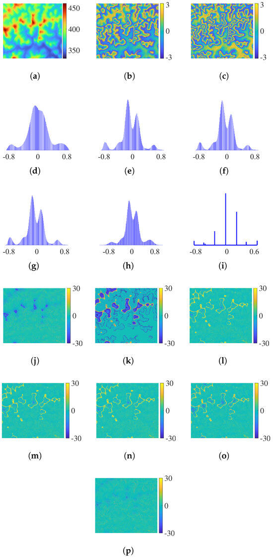
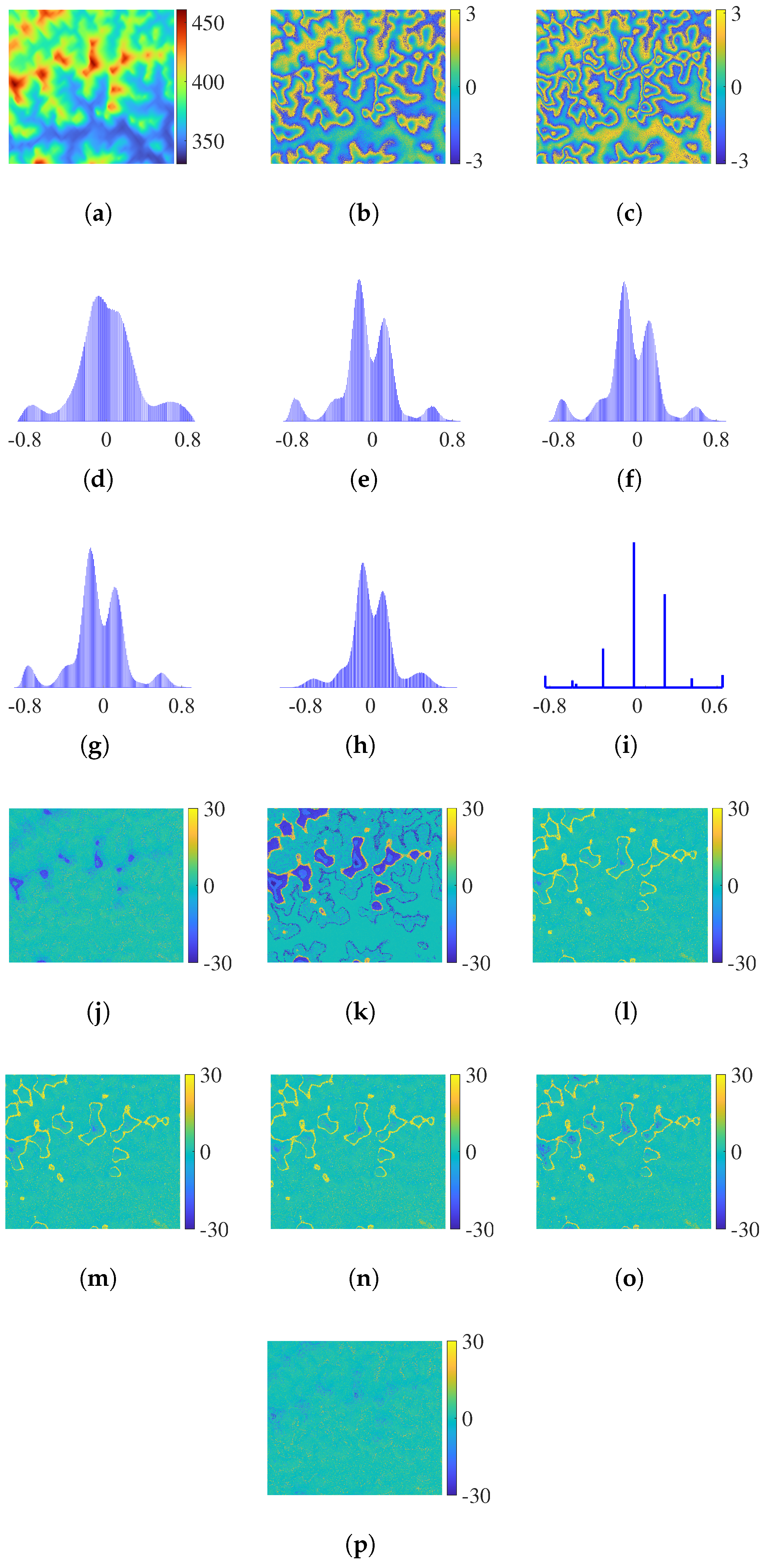
The simulation data experiment adopts a one-transmitter, three-receiver dual-baseline InSAR mode. Specific parameters are detailed in Table 2. It aims to verify the unwrapping accuracy, computational efficiency, and noise robustness of the proposed algorithm. The pixel size of the experimental data is 1240 × 1271 pixels. Specifically, the vertical effective baseline lengths of Baseline 1 and Baseline 2 are 297.63 m and 401.16 m, respectively, corresponding to ambiguity heights of 43.53 m and 32.31 m in sequence; the radar look angle is 40°, the satellite orbit altitude is 500 km, and the carrier signal frequency is 9.65 GHz. The azimuth resolution is 3 m, the range resolution is 2 m, the signal bandwidth is 72 MHz, the pulse repetition frequency (PRF) is 3100 Hz, and the multilook factor is set to 1. The observation scene is shown in Figure 5a, with a maximum height of 460.75 m and a minimum height of 330.31 m. To simulate noise interference, Gaussian white noise with a standard deviation of 0.9 rad is added to the data. The noisy interferometric phases for the two baselines are displayed in Figure 5b and Figure 5c, respectively.

Table 2. Specification table of simulation data experiment.

Working Mode	One-Transmitter, Three-Receiver Dual-Baseline Mode
pixel size	1240 × 1271
$B_1$	297.63 m
$B_2$	401.16 m
ambiguity height of Baseline 1	43.53 m
ambiguity height of Baseline 2	32.31 m
radar look angle	${40}^{\circ }$
satellite orbit altitude	500 km
carrier signal frequency	9.65 GHz
azimuth resolution	3 m
range resolution	2 m
bandwidth	72 MHz
pulse repetition frequency (PRF)	3100 Hz
multilook	1

Figure 5. (a) Reference DEM (unit: m). (b) Noisy interferometric phase of $B_1$ with 0.9 rad noise (unit: rad). (c) Noisy interferometric phase of $B_2$ with 0.9 rad noise (unit: rad). (d) Intercept distribution without pre-filtering. (e) Intercept distribution of PPCC. (f) Intercept distribution of NPCC1. (g) Intercept distribution of NPCC2. (h) Intercept distribution of BM3D. (i) Intercept distribution of the proposed algorithm. (j) Reconstructed phase error of RPIP (unit: rad). (k) Reconstructed phase error without pre-filtering (unit: rad). (l) Reconstructed phase error of PPCC (unit: rad). (m) Reconstructed phase error of NPCC1 (unit: rad). (n) Reconstructed phase error of NPCC2 (unit: rad). (o) Reconstructed phase error of BM3D (unit: rad). (p) Reconstructed phase error of the proposed algorithm (unit: rad).

Figure 5j shows the reconstructed phase error result of RPIP. Obvious errors are observed, mainly because phase noise causes mistakes in integer search, leading to unwrapping errors. Figure 5d presents the original intercept distribution without pre-filtering, while Figure 5k shows the corresponding reconstructed phase error result. As can be clearly observed, the original intercept distribution is highly disorganised and chaotic due to the influence of severe phase noise. Such chaotic distribution characteristics directly lead to large-scale and severe phase unwrapping errors in the subsequent reconstruction process, which seriously degrade the accuracy and reliability of the unwrapped phase. Figure 5e–h depict the intercept distributions after pre-filtering using four comparative algorithms: PPCC, NPCC1, NPCC2 and BM3D. For all intercept distribution histograms, the actual intercept values are quantised to two or three decimal places. The vertical axis represents the raw, unnormalised sample count. Compared with the disordered distribution in Figure 5d, the intercept distributions after pre-filtering show significantly clearer boundaries between different cluster groups and greatly improved structural regularity. The noise interference is effectively suppressed, and the aggregation and separation characteristics of the intercepts become more distinct, which is beneficial to accurate phase unwrapping. Figure 5l–o show the reconstructed phase error results corresponding to the above four intercept pre-filtering algorithms. Although all these algorithms achieve significant performance improvement over the case without pre-filtering and greatly reduce the overall phase error, local errors still remain in the reconstructed results. These residual errors are mainly caused by the loss of weak cluster groups or the offset of cluster centerlines, which further degrade the continuity and accuracy of phase unwrapping in local regions.

Figure 5i illustrates the intercept distribution of the proposed algorithm, which exhibits a clearer and more complete distribution compared with those of other algorithms. As can be clearly seen from the distribution characteristics, the intercept pre-filtering strategy designed in the proposed algorithm performs accurate correction on the intercept values of all pixels based on the reference intercept vector with strict physical constraints. This advanced pre-filtering mechanism not only ensures the complete preservation of all cluster groups but also effectively prevents weak cluster groups from being merged by noise and avoids the overlap of adjacent cluster groups caused by actual intercept distortion. Correspondingly, Figure 5p shows the reconstructed phase error result of the proposed algorithm. It is evident that the reconstructed phase error distribution of the proposed algorithm is significantly suppressed in both error range and error intensity, exhibiting a substantially lower error rate compared with the RPIP algorithm, the algorithm without pre-filtering and the other four comparative algorithms. This fully reflects the effectiveness of the proposed algorithm in improving phase unwrapping accuracy.

Table 3 systematically quantifies the performance of all algorithms in the simulation data experiment from three evaluation metrics: phase unwrapping success rate (PUSR), root mean square error (RMSE), and running time. In terms of accuracy, the algorithm without pre-filtering performs the worst, achieving the PUSR of only 80.17% and the RMSE as high as 7.93 rad. The RPIP algorithm achieves moderate accuracy, with a PUSR of 89.97% and an RMSE of 4.88 rad. The four traditional pre-filtering algorithms (PPCC, NPCC1, NPCC2 and BM3D) exhibit moderate accuracy improvements: their PUSR ranges from 89.39% (BM3D) to 90.43% (PPCC), and their RMSE is reduced to between 4.39 rad (PPCC) and 4.90 rad (BM3D). In contrast, the proposed algorithm achieves the optimal accuracy performance, with the highest PUSR of 94.59% and the lowest RMSE of 2.76 rad, demonstrating its superior ability to preserve cluster groups and reduce phase unwrapping errors. In terms of efficiency, the computational cost varies significantly among different algorithms. The algorithm without pre-filtering takes 37.89 s, while the traditional pre-filtering algorithms require more computational time, ranging from 44.32 s (NPCC2) to 45.33 s (PPCC), due to the additional pre-filtering step. The RPIP algorithm takes 22.33 s. Remarkably, the proposed algorithm achieves an ultra-low running time of 13.28 s, which is not only far shorter than all traditional pre-filtering algorithms but also significantly faster than the algorithm without pre-filtering. Meanwhile, the proposed algorithm is also more efficient than the RPIP algorithm, whose main time consumption lies in the integer search along a specific direction. This efficiency advantage stems from the integrated processing of intercept pre-filtering and ambiguity number vector determination. Leveraging the strict one-to-one mapping relationship between reference intercepts and ambiguity number combinations, the algorithm directly derives the ambiguity number vector. It eliminates the time-consuming intercept peak search and ambiguity number search processes inherent in traditional CA algorithms.

Table 3. Accuracy and efficiency statistics of simulation data experiment.

	PUSR	RMSE (Unit: rad)	Time (Unit: s)
RPIP	89.97%	4.88	22.33
Without pre-filtering	80.17%	7.93	37.89
PPCC	90.43%	4.39	45.33
NPCC1	90.13%	4.57	45.29
NPCC2	90.01%	4.68	44.32
BM3D	89.39%	4.90	44.61
Proposed algorithm	94.59%	2.76	13.28

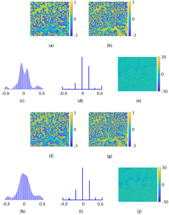
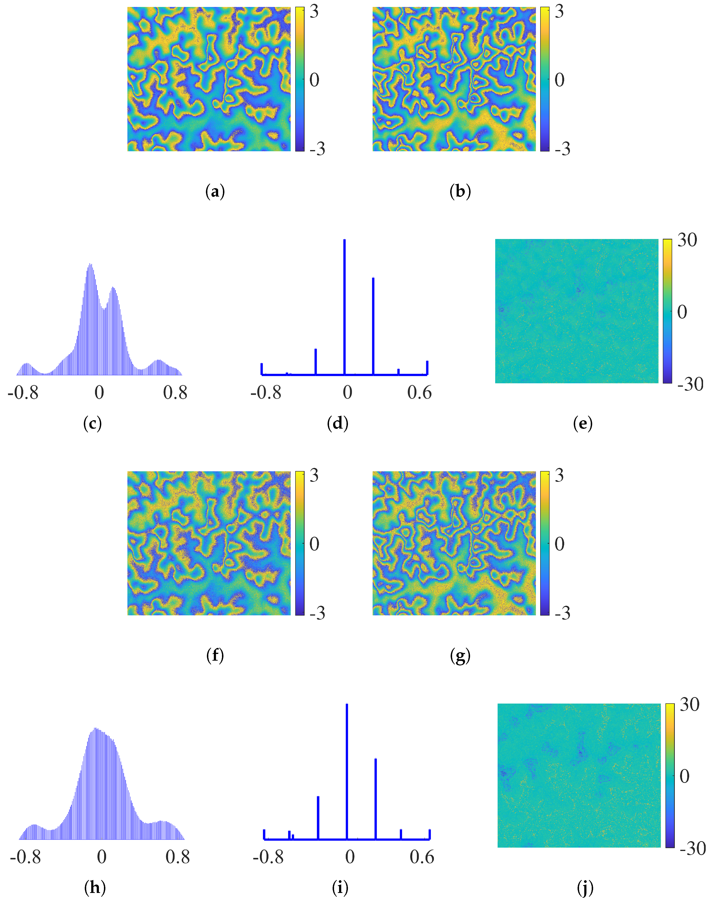
To verify the proposed algorithm’s robustness under different noise conditions, the simulation data experiment added two datasets with 0.6 rad and 1.2 rad Gaussian white noise, with results in Figure 6 and Table 4. As shown in Figure 5d and Figure 6c,h, the intercept distribution without pre-filtering deteriorates sharply as the noise intensity increases from 0.6 rad and 0.9 rad to 1.2 rad. In contrast, the intercept distribution of the proposed algorithm (Figure 5i and Figure 6d,i) retains clear boundaries and an intact structure across all three noise levels, attributed to its precise pre-filtering strategy anchored in physically constrained reference intercept vectors. Correspondingly, the reconstructed phase errors of the proposed algorithm (Figure 5o and Figure 6e,j) exhibit acceptable fluctuation, and the quantitative data in Table 4 further corroborates the algorithm’s robustness under varying noise conditions.

Figure 6. (a) Noisy interferometric phase of $B_1$ with 0.6 rad noise (unit: rad). (b) Noisy interferometric phase of $B_2$ with 0.6 rad noise (unit: rad). (c) Intercept distribution without pre-filtering with 0.6 rad noise. (d) Intercept distribution of the proposed algorithm with 0.6 rad noise. (e) Reconstructed phase error of the proposed algorithm with 0.6 rad noise (unit: rad). (f) Noisy interferometric phase of $B_1$ with 1.2 rad noise (unit: rad). (g) Noisy interferometric phase of $B_2$ with 1.2 rad noise (unit: rad). (h) Intercept distribution without pre-filtering with 1.2 rad noise. (i) Intercept distribution of the proposed algorithm with 1.2 rad noise. (j) Reconstructed phase error of the proposed algorithm with 1.2 rad noise (unit: rad).

Table 4. Accuracy and efficiency statistics of the proposed algorithm under three noise levels.

Added Phase Noise (rad)	PUSR	RMSE (Unit: rad)	Time (Unit: s)
0.6	94.97%	2.49	13.21
0.9	94.59%	2.76	13.28
1.2	94.17%	2.93	13.27

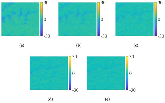
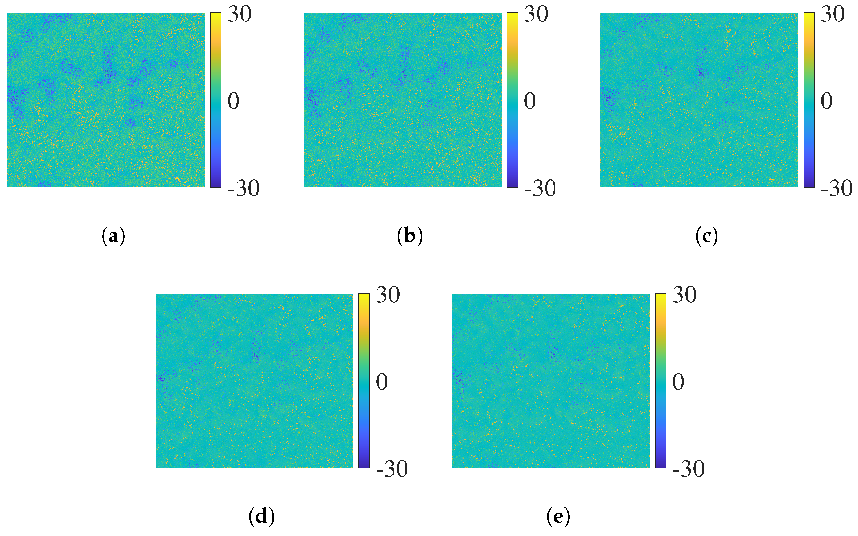
To comprehensively verify the performance of the proposed algorithm under different window sizes, experiments are carried out at a phase noise level of 0.9 rad using five window configurations: 3 × 3, 5 × 5, 7 × 7, 9 × 9, and 11 × 11. Figure 7a–e show the reconstructed phase error results for the various window sizes. As the window size increases, it can be seen that the phase error decreases progressively. The quantitative results are summarised in Table 5: both PUSR and RMSE are continuously optimised with larger window sizes. The main reason for this is that a larger window incorporates more neighbouring pixels, which effectively suppresses the noise interference of individual pixels and significantly improves the robustness of phase unwrapping. However, in terms of computational efficiency, the runtime increases significantly with the expansion of the window size. Further analysis shows that an excessively small window fails to suppress noise effectively, which directly degrades the unwrapping accuracy. Conversely, an overly large window, despite its superior noise reduction performance, leads to reduced computational efficiency and enhanced spatial averaging effects. This results in the loss of detailed terrain features. Therefore, selecting an appropriate window size requires a balance to be struck between accuracy, efficiency, and detail preservation, and the optimal configuration should be determined according to the requirements of the practical application.

Figure 7. Reconstructed phase error of the proposed algorithm under 0.9 rad phase noise for different window sizes. (a) Reconstructed phase error of 3 × 3 window size (unit: rad). (b) Reconstructed phase error of 5 × 5 window size (unit: rad). (c) Reconstructed phase error of 7 × 7 window size (unit: rad). (d) Reconstructed phase error of 9 × 9 window size (unit: rad). (e) Reconstructed phase error of 11 × 11 window size (unit: rad).

Table 5. Performance of the proposed algorithm under 0.9 rad phase noise with different window sizes.

Window Size	PUSR	RMSE (Unit: rad)	Time (Unit: s)
3 × 3	93.13%	3.32	10.85
5 × 5	93.87%	3.07	11.99
7 × 7	94.59%	2.76	13.28
9 × 9	94.93%	2.51	15.01
11 × 11	95.37%	2.39	18.04

4.2. Real Data Experiment

This experiment employs dual-baseline InSAR real data acquired by the TanDEM-X system. Each baseline has an independent transmit–receive link. The goal is to verify the proposed algorithm’s adaptability to complex real terrain and practical observation noise. Detailed specifications of the experimental system and parameters are presented in Table 6, with the experimental data sized at 1001 × 501 pixels. The vertical effective baseline lengths of the two baselines are 82.97 m and 107.55 m, corresponding to ambiguity heights of 55.33 m and 42.71 m, respectively; the radar look angles of the two baselines are 32.181° and 32.123°, respectively. The carrier signal frequency is 9.65 GHz, the azimuth resolution is 3.3 m, the range resolution is 1.7 m, the signal bandwidth is 80 MHz, the PRF is 4137 Hz, and the multilook factor is set to 1. In this experiment, the comparative algorithms all adopt an elevation search range of 0 m to 2000 m for ambiguity numbers. In addition, the calibrated high-resolution TanDEM-X DEM is adopted as the reference DEM product, and its elevation accuracy in the observation area meets the requirements of experimental accuracy evaluation.

Table 6. Specification table of real data experiment.

Working Mode	Dual-Baseline Architecture, with Each Baseline Equipped with an Independent Transmit–Receive Link
pixel size	1001 × 501
$B_1$	82.97 m
$B_2$	107.55 m
ambiguity height of Baseline 1	55.33 m
ambiguity height of Baseline 2	42.71 m
radar look angle of Baseline 1	$32.{181}^{\circ }$
radar look angle of Baseline 2	$32.{123}^{\circ }$
observation time of Baseline 1	17 January 2013
observation time of Baseline 2	15 December 2012
carrier signal frequency	9.65 GHz
azimuth resolution	3.3 m
range resolution	1.7 m
bandwidth	80 MHz
PRF	4137 Hz
multilook	1

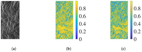
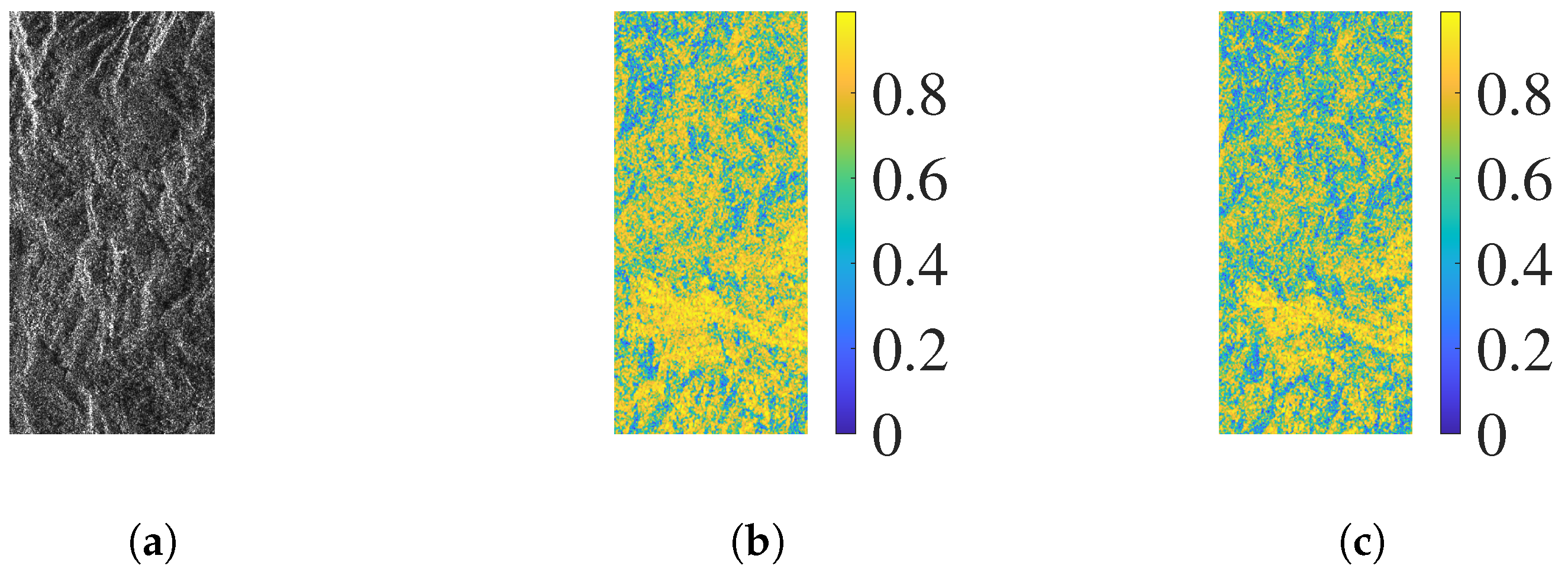
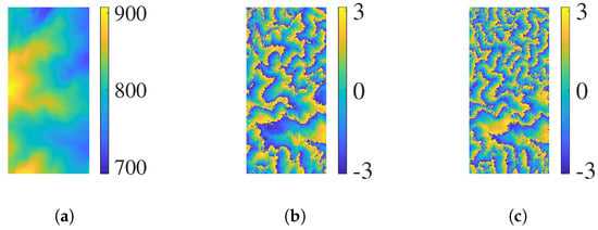
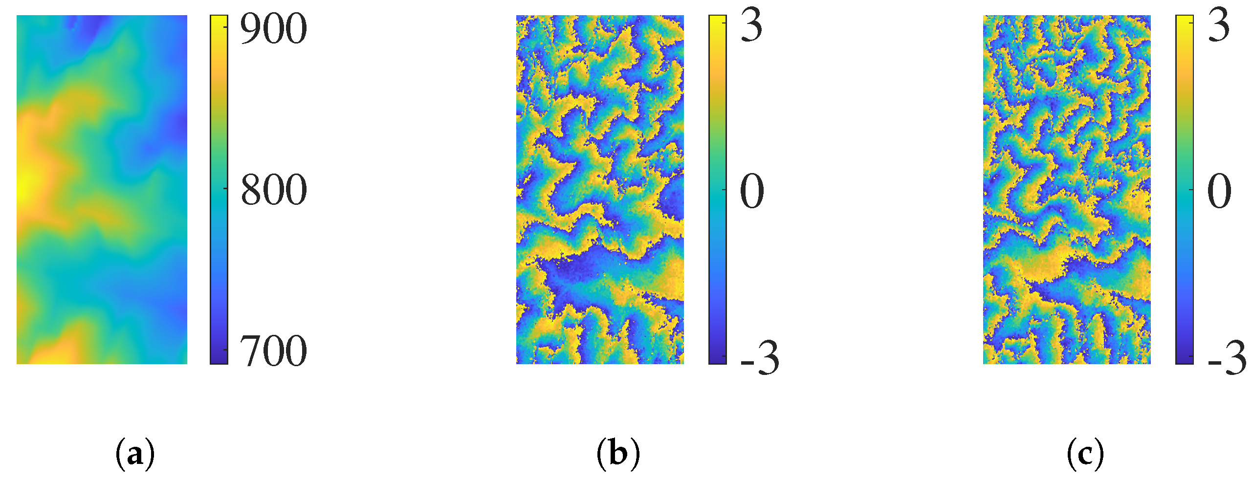
The observation area is located around Mount Lawu in Indonesia, with a topographic elevation range of 709.08 m to 908.37 m. Figure 8a shows the intensity image of the observed area, while Figure 8b and Figure 8c present the coherences corresponding to Baseline 1 and Baseline 2, respectively. As illustrated in Figure 9a, the reference DEM of the observation area exhibits typical complex terrain characteristics, which can effectively verify the algorithm’s adaptability to actual topographic conditions. Figure 9b and Figure 9c present the interferometric phases of Baseline 1 and Baseline 2, respectively.

Figure 8. (a) Intensity image. (b) Coherence of $B_1$. (c) Coherence of $B_2$.

Figure 9. (a) Reference DEM (unit: m). (b) Interferometric phase of $B_1$ (unit: rad). (c) Interferometric phase of $B_2$ (unit: rad).

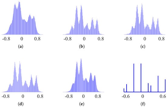
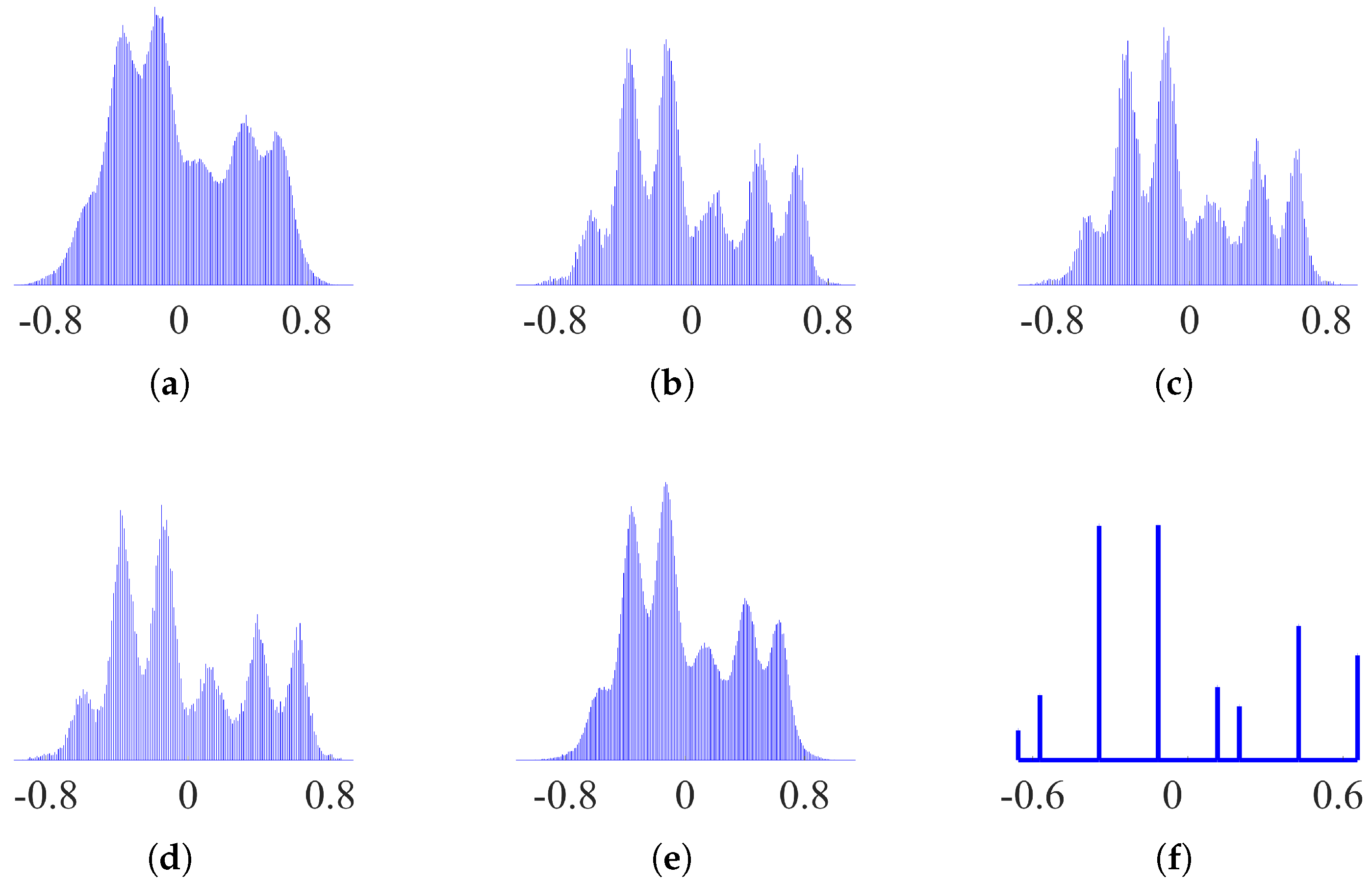
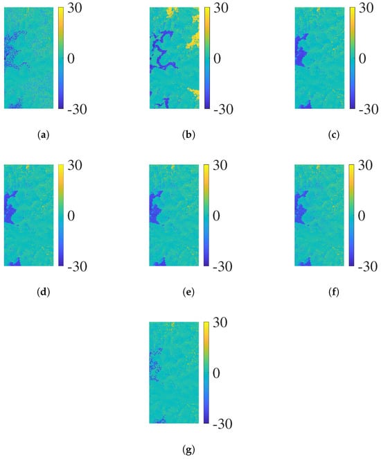
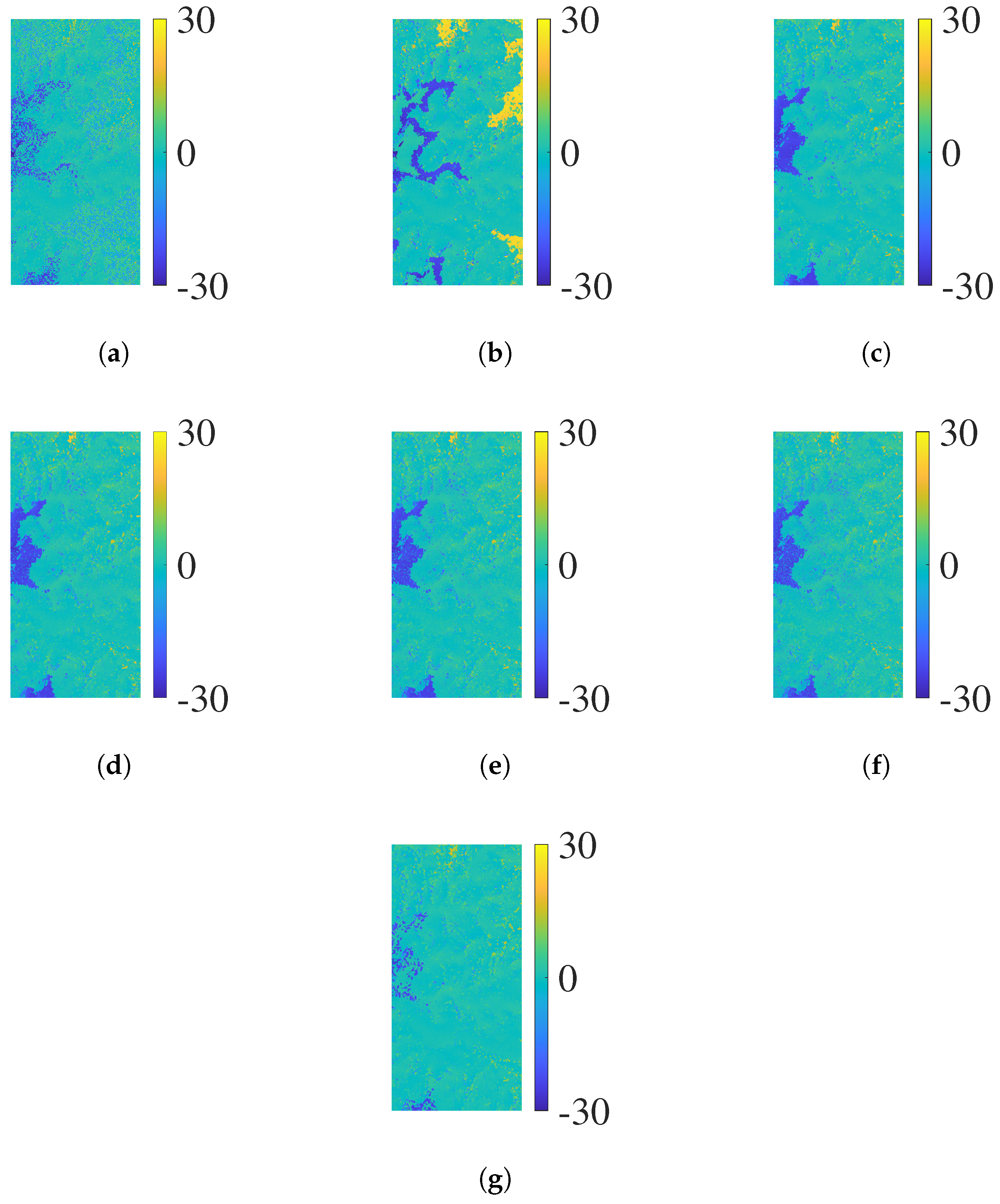
Figure 10 presents the intercept distribution results of the without pre-filtering algorithm, four traditional algorithms (PPCC, NPCC1, NPCC2 and BM3D), and the proposed algorithm. The original intercept distribution without pre-filtering (Figure 10a) is severely distorted by noise, with blurred cluster boundaries, obvious overlaps, and partial weak cluster groups submerged. Although the four traditional algorithms (Figure 10b–e) significantly improve the regularity of intercept distribution and achieve remarkable noise reduction effects. By virtue of the precise pre-filtering strategy based on physically constrained reference intercept vectors, the proposed algorithm (Figure 10f) maintains clear cluster boundaries and intact structures, avoiding cluster group overlaps and weak cluster group loss caused by noise. Figure 11 shows the reconstructed phase error results of each algorithm, intuitively reflecting their phase unwrapping performance. Figure 11a shows the reconstructed phase error result of the RPIP algorithm, where several error regions can be observed. Figure 11b indicates that the algorithm without pre-filtering has disordered errors and many obvious phase jumps, leading to poor unwrapping effects. The four traditional pre-filtering algorithms (PPCC, NPCC1, NPCC2 and BM3D) in Figure 11c–f effectively reduce errors compared with the algorithm without pre-filtering but still have regional residual errors, limiting local unwrapping accuracy. In contrast, the proposed algorithm in Figure 11g achieves optimal performance, with significantly suppressed phase errors and remarkably excellent unwrapping accuracy and stability.

Figure 10. (a) Intercept distribution without pre-filtering. (b) Intercept distribution of PPCC. (c) Intercept distribution of NPCC1. (d) Intercept distribution of NPCC2. (e) Intercept distribution of BM3D. (f) Intercept distribution of the proposed algorithm.

Figure 11. (a) Reconstructed phase error of RPIP (unit: rad). (b) Reconstructed phase error without pre-filtering (unit: rad). (c) Reconstructed phase error of PPCC (unit: rad). (d) Reconstructed phase error of NPCC1 (unit: rad). (e) Reconstructed phase error of NPCC2 (unit: rad). (f) Reconstructed phase error of BM3D (unit: rad). (g) Reconstructed phase error of the proposed algorithm (unit: rad).

Table 7 quantitatively evaluates the performance of each algorithm through PUSR, RMSE and running time, further verifying the accuracy and efficiency advantages of the proposed algorithm. During the accuracy evaluation, invalid regions such as shadowed and severely layover-affected areas are excluded from the analysis. In terms of unwrapping accuracy, the algorithm without pre-filtering performs the worst, with a PUSR of only 87.67% and an RMSE as high as 6.76 rad. The RPIP algorithm achieves moderate accuracy, with a PUSR of 90.01% and an RMSE of 4.96 rad. The four traditional algorithms (PPCC, NPCC1, NPCC2 and BM3D) achieve moderate accuracy improvement, with PUSR ranging from 90.06% (BM3D) to 90.61% (PPCC) and RMSE between 4.70 rad (PPCC) and 4.93 rad (BM3D), showing slight performance differences. In contrast, the proposed algorithm exhibits significantly superior accuracy, with the PUSR of 95.71% and the RMSE of only 2.79 rad. Regarding computational efficiency, the algorithm without pre-filtering takes 23.19 s, while the four traditional algorithms require 29.16 s (NPCC1) to 29.30 s (PPCC) due to the additional pre-filtering step. The RPIP algorithm takes 14.78 s. The proposed algorithm completes the processing in only 8.28 s, and its efficiency advantage stems from the integrated processing of intercept pre-filtering and ambiguity number vector determination, which eliminates the time-consuming intercept peak search and ambiguity number search processes in comparative algorithms. In summary, the proposed algorithm outperforms all comparative algorithms, including five CA-based algorithms and the newly proposed RPIP algorithm, in terms of both accuracy and efficiency.

Table 7. Accuracy and efficiency statistics of real data experiment.

	PUSR	RMSE (Unit: rad)	Time (Unit: s)
RPIP	90.01%	4.96	14.78
Without pre-filtering	87.67%	6.76	23.19
PPCC	90.61%	4.70	29.30
NPCC1	90.22%	4.73	29.16
NPCC2	90.20%	4.79	29.18
BM3D	90.06%	4.93	29.29
proposed algorithm	95.71%	2.79	8.28

5. Conclusions

This article proposes a multi-baseline phase unwrapping algorithm based on the integrated processing of intercept pre-filtering and ambiguity number vector determination, aiming to solve the issues of cluster group loss, cluster centerline offset, and low computational efficiency in traditional CA-based multi-baseline phase unwrapping algorithms. Four core technical optimisations enhance its performance. First, the linear relationship model of ambiguity numbers is extended and reconstructed to be compatible with both traditional one-transmitter, multi-receiver multi-baseline InSAR systems and distributed multi-baseline InSAR systems with independent transmit–receive links, thus breaking the application limitations of the original model. Second, a strict one-to-one mapping relationship between reference intercepts and ambiguity number combinations is derived, established, and verified, laying a theoretical foundation for their direct mutual derivation. Third, a double constraints screening strategy for ambiguity number combinations is designed to accurately filter out valid ambiguity number combinations with physical rationality, ensuring the reliability of the reference intercept vector. Fourth, an intercept pre-filtering method based on the reference intercept vector is constructed to realise the integrated processing of actual intercept pre-filtering and ambiguity number vector determination, thus eliminating the time-consuming search steps in traditional CA algorithms. The simulation data experiment under varying noise levels and real data experiment collectively validates the effectiveness of the proposed algorithm. Compared with the algorithm without pre-filtering and traditional intercept pre-filtering algorithms, the proposed algorithm demonstrates significant superiority in unwrapping accuracy and computational efficiency. Future research will focus on optimising the algorithm’s lightweight processing capability for large-scale scenes and exploring its integration with deep learning technologies, aiming to further enhance its adaptability and practicality for diverse complex InSAR data processing scenarios.

References

- Bamler, R.; Hartl, P. Synthetic Aperture Radar Interferometry. Inverse Probl. 1998, 14, R1–R54. [Google Scholar] [CrossRef] [Scilit]
- Gao, Y.; Yao, J.; Zhou, W.; Zheng, N.; Li, S.; Tian, Y. CBIPDNet: A Novel Method for InSAR Deformation Interferometric Phase Filtering Using Deep Learning Network. IEEE J. Sel. Top. Appl. Earth Obs. Remote Sens. 2024, 17, 15806–15815. [Google Scholar] [CrossRef] [Scilit]
- Yuan, Z.; Chen, T.; Xing, X.; Peng, W.; Chen, L. BM3D Denoising for a Cluster-Analysis-Based Multibaseline InSAR Phase-Unwrapping Method. Remote Sens. 2022, 14, 1836. [Google Scholar] [CrossRef] [Scilit]
- Zhao, J.; Wu, J.; Ding, X.; Wang, M. Elevation Extraction and Deformation Monitoring by Multitemporal InSAR of Lupu Bridge in Shanghai. Remote Sens. 2017, 9, 897. [Google Scholar] [CrossRef] [Scilit]
- Yan, Y.; Yu, H.; Yang, T. A Multitemporal Baseline Phase Unwrapping Approach for Accurately Monitoring High-Gradient Deformation With Two-Pass DInSAR. IEEE Trans. Geosci. Remote Sens. 2025, 63, 1–12. [Google Scholar] [CrossRef] [Scilit]
- Zeng, P.; Feng, B.; Dai, K.; Li, T.; Fan, X.; Sun, X. Can Satellite InSAR Innovate the Way of Large Landslide Early Warning? Eng. Geol. 2024, 342, 107771. [Google Scholar] [CrossRef] [Scilit]
- Ding, Q.; Shao, Z.; Huang, X.; Altan, O.; Zhuang, Q.; Hu, B. Monitoring, Analyzing and Predicting Urban Surface Subsidence: A Case Study of Wuhan City, China. Int. J. Appl. Earth Obs. Geoinf. 2021, 102, 102422. [Google Scholar] [CrossRef] [Scilit]
- Sun, Z.; Liu, L.; Fan, C.; Hu, Y.; Baldacchino, F.; Bhattacharya, A.; Wood, E.; Bolch, T. Unveiling Large-Scale Velocity Characteristics of Rock Glaciers in the Tibet-Pamir-Karakoram Region Using InSAR. Int. J. Appl. Earth Obs. Geoinf. 2025, 142, 104733. [Google Scholar] [CrossRef] [Scilit]
- Rosen, P.A.; Hensley, S.; Joughin, I.R.; Li, F.K.; Madsen, S.N.; Rodriguez, E.; Goldstein, R.M. Synthetic Aperture Radar Interferometry. Proc. IEEE 2000, 88, 333–382. [Google Scholar] [CrossRef] [Scilit]
- Lattari, F.; Cannici, M.; Murdaca, G.; Rucci, A.; Prati, C.M.; Matteucci, M. NeuralPUMA: Learning to Phase Unwrap Through Differentiable Graph Cuts. IEEE Trans. Signal Process. 2024, 72, 321–336. [Google Scholar] [CrossRef] [Scilit]
- Yang, Y.; Chen, B.; Li, Z.; Yu, C.; Song, C.; Guo, F. A Novel Phase Unwrapping Method for Low Coherence Interferograms in Coal Mining Areas Based on a Fully Convolutional Neural Network. IEEE J. Sel. Top. Appl. Earth Obs. Remote Sens. 2024, 17, 601–613. [Google Scholar] [CrossRef] [Scilit]
- Ye, X.; Yu, H. A Novel Loss Function for Deep Learning-Based One-Step Phase Unwrapping. In Proceedings of the IGARSS 2024—2024 IEEE International Geoscience and Remote Sensing Symposium, Athens, Greece, 7–12 July 2024; pp. 3498–3501. [Google Scholar] [CrossRef] [Scilit]
- Zhou, L.; Yu, H. InSAR-DLPU: A Benchmark Dataset for Deep Learning-Based Synthetic Aperture Radar Interferometry Phase Unwrapping [Software and Data Sets]. IEEE Geosci. Remote Sens. Mag. 2024, 12, 118–124. [Google Scholar] [CrossRef] [Scilit]
- Yu, H.; Lan, Y.; Yuan, Z.; Xu, J.; Lee, H. Phase Unwrapping in InSAR: A Review. IEEE Geosci. Remote Sens. Mag. 2019, 7, 40–58. [Google Scholar] [CrossRef] [Scilit]
- Jia, Y.; Gao, Y.; Zhang, S.; Li, S.; Zhang, Y.; Li, M. A Novel 2-D Phase Unwrapping Method Based on PUMA for Aerospace Topographic Mapping Systems. IEEE J. Miniaturization Air Space Syst. 2022, 3, 113–120. [Google Scholar] [CrossRef] [Scilit]
- Yang, K.; Yuan, Z.; Xing, X.; Chen, L. Deep-Learning-Based Mask-Cut Method for InSAR Phase Unwrapping. IEEE J. Miniaturization Air Space Syst. 2023, 4, 221–230. [Google Scholar] [CrossRef] [Scilit]
- Yuan, Z.; Wang, Z.; Chen, L.; Xing, X. A Multibaseline Insar Phase Unwrapping Algorithm Based On Wavelet Clustering. In Proceedings of the IGARSS 2023—2023 IEEE International Geoscience and Remote Sensing Symposium, Pasadena, CA, USA, 16–21 July 2023; pp. 7977–7980. [Google Scholar] [CrossRef] [Scilit]
- Lan, Y.; Yu, H.; Xing, M.; Plaza, A. A Cluster-Analysis and Convex Hull-Based Fast Large-Scale Phase Unwrapping Method for Single- and Multibaseline SAR Interferograms. IEEE J. Sel. Top. Appl. Earth Obs. Remote Sens. 2023, 16, 5416–5429. [Google Scholar] [CrossRef] [Scilit]
- Yan, Y.; Yu, H.; Yang, T. Two-Dimensional Phase Unwrapping for Topography Reconstruction: A Refined Two-Stage Programming Approach. IEEE J. Sel. Top. Appl. Earth Obs. Remote Sens. 2024, 17, 20304–20314. [Google Scholar] [CrossRef] [Scilit]
- Xu, W.; Chang, E.C.; Kwoh, L.K.; Lim, H.; Cheng, W.; Heng, A. Phase-Unwrapping of SAR Interferogram with Multi-Frequency or Multi-Baseline. In Proceedings of the IGARSS ’94—1994 IEEE International Geoscience and Remote Sensing Symposium, Pasadena, CA, USA, 8–12 August 1994; Volume 2, pp. 730–732. [Google Scholar] [CrossRef] [Scilit]
- Xia, X.; Wang, G. Phase Unwrapping and A Robust Chinese Remainder Theorem. IEEE Signal Process. Lett. 2007, 14, 247–250. [Google Scholar] [CrossRef] [Scilit]
- Wang, W.; Xia, X. A Closed-Form Robust Chinese Remainder Theorem and Its Performance Analysis. IEEE Trans. Signal Process. 2010, 58, 5655–5666. [Google Scholar] [CrossRef] [Scilit]
- Yuan, Z.; Deng, Y.; Li, F.; Wang, R.; Liu, G.; Han, X. Multichannel InSAR DEM Reconstruction Through Improved Closed-Form Robust Chinese Remainder Theorem. IEEE Geosci. Remote Sens. Lett. 2013, 10, 1314–1318. [Google Scholar] [CrossRef] [Scilit]
- Yu, H.; Li, Z.; Bao, Z. A Cluster-Analysis-Based Efficient Multibaseline Phase-Unwrapping Algorithm. IEEE Trans. Geosci. Remote Sens. 2011, 49, 478–487. [Google Scholar] [CrossRef] [Scilit]
- Liu, H.; Xing, M.; Bao, Z. A Cluster-Analysis-Based Noise-Robust Phase-Unwrapping Algorithm for Multibaseline Interferograms. IEEE Trans. Geosci. Remote Sens. 2015, 53, 494–504. [Google Scholar] [CrossRef] [Scilit]
- Yuan, Z.; Lu, Z.; Chen, L.; Xing, X. A Closed-Form Robust Cluster-Analysis-Based Multibaseline InSAR Phase Unwrapping and Filtering Algorithm With Optimal Baseline Combination Analysis. IEEE Trans. Geosci. Remote Sens. 2020, 58, 4251–4262. [Google Scholar] [CrossRef] [Scilit]
- Yuan, Z.; Chen, T.; Yu, H.; Peng, W.; Chen, L.; Xing, X. Cluster Correction for Cluster Analysis-Based Multibaseline InSAR Phase Unwrapping. IEEE J. Sel. Top. Appl. Earth Obs. Remote Sens. 2022, 15, 8600–8612. [Google Scholar] [CrossRef] [Scilit]
- Zhou, L.; Yu, H.; Lan, Y.; Gong, S.; Xing, M. CANet: An Unsupervised Deep Convolutional Neural Network for Efficient Cluster-Analysis-Based Multibaseline InSAR Phase Unwrapping. IEEE Trans. Geosci. Remote Sens. 2022, 60, 1–15. [Google Scholar] [CrossRef] [Scilit]
- Liu, H.; Zheng, K.; Miao, C.; Liu, X.; Liu, X.; Li, L.; Zhang, Y.; Xiong, L. PIPNet: A Deep Convolutional Neural Network for Multibaseline InSAR Phase Unwrapping Based on Pure Integer Programming. IEEE J. Sel. Top. Appl. Earth Obs. Remote Sens. 2025, 18, 15495–15507. [Google Scholar] [CrossRef] [Scilit]
- Yue, J.; Huang, Q.; Liu, H.; He, Z.; Zhang, H. Multibaseline Phase Unwrapping With a Refined Parametric Pure Integer Programming for Noise Suppression. IEEE J. Miniat. Air Space Syst. 2024, 5, 156–164. [Google Scholar] [CrossRef] [Scilit]
- Li, X.; Dongsun, H.; Yuan, Z.; Yu, H. Multichannel InSAR DEM Reconstruction Using Robust Redundancy Residue Number Systems. IEEE Trans. Geosci. Remote Sens. 2025, 63, 1–10. [Google Scholar] [CrossRef] [Scilit]
Disclaimer/Publisher’s Note: The statements, opinions and data contained in all publications are solely those of the individual author(s) and contributor(s) and not of MDPI and/or the editor(s). MDPI and/or the editor(s) disclaim responsibility for any injury to people or property resulting from any ideas, methods, instructions or products referred to in the content. |
© 2026 by the authors. Licensee MDPI, Basel, Switzerland. This article is an open access article distributed under the terms and conditions of the Creative Commons Attribution (CC BY) license.