


Highlights
What are the main findings?
- Based on in situ data, phytoplankton absorption correlates well with Chl-a; R2 was stronger in the red spectral region (670 nm).
- Accuracy of the satellite retrieval of apig, using C2RCC, is low for both Sentinel-2 and Sentinel-3.
What are the implications of the main findings?
- Low R2 and high error metrics of apig indicate the need for enhancements in the performance of C2RCC.
- OWT-specific approach to derive Chl-a from apig data may be beneficial, but only if satellite detection of apig improves significantly.
Abstract
Accurate detection of chlorophyll-a (Chl-a) is critical for monitoring water quality in inland waters, where high concentrations of coloured dissolved organic matter (CDOM) complicate retrieval process. Reliable Chl-a estimation depends on the precise determination of the phytoplankton absorption coefficient (aph). This study evaluates Chl-a detection from in situ aph measurements and assesses the accuracy of phytoplankton absorption retrieval from Sentinel-2/MSI (S2) and Sentinel-3/OLCI (S3) using the Case-2-Regional-Coast-Colour (C2RCC) processor across diverse optical water types (OWTs) in boreal lakes. OWTs were classified based on remote sensing reflectance features, representing Clear, Moderate, Turbid, Very Turbid, and Brown conditions. CDOM absorption strongly influenced the underwater light field, particularly in Brown and Turbid waters. Linear relationships between aph and Chl-a were generally strong across OWTs, with improved relationships in the red spectral region (670 nm). Satellite-derived apig estimates showed a weak relationship with in situ data (R2 = 0.26–0.45). Both sensors overestimated small aph values, while S3 underestimated larger ones. S2 underestimated aph in Clear and Brown OWTs, with median absolute percentage differences near 100% for all OWTs. These findings emphasize the challenges posed by bio-optical complexity in boreal lakes and highlight the need for OWT-specific algorithms to improve satellite-based absorption and Chl-a retrieval accuracy.
Keywords:
phytoplankton absorption; optical water types; Sentinel 3/OLCI; Sentinel 2/MSI; C2RCC; WFD 1. Introduction
Phytoplankton are a key element in aquatic food chains and are often characterized by the amount of the main photosynthetic pigment, chlorophyll-a (Chl-a). Phytoplankton pigment absorption (aph) is an important parameter in models for remote sensing retrieval of Chl-a, whose determination using remote sensing methods remains challenging in turbid inland and coastal waters [1,2]. In these optically complex waters, light is absorbed not only by phytoplankton, as is typical in the open ocean, but also by various organic and mineral substances that do not correlate with each other, making accurate detection of Chl-a and phytoplankton-specific grouping difficult. The magnitude of aph varies with pigment concentration, with additional variability introduced by the pigment packaging effect [3]. Understanding the spectral, temporal, and spatial variability of phytoplankton absorption is essential to enhancing knowledge on phytoplankton ecological variability and to improving satellite-based detection in optically complex inland waters.
The Water Framework Directive (WFD, Directive 2000/60/EC) requires the monitoring of and reporting on the ecological status of all lakes larger than 0.5 km2—an initiative and obligation that have led to a stronger focus on lakes, including setting the classification of lake types and characterizing their ecological status on a European scale Phytoplankton are the central biological element; assessments in various European countries include Chl-a concentration, phytoplankton biomass, biomass of specific groups, taxonomic composition, focus on species preferring specific conditions, and indices based on taxonomic composition [4,5]. Currently, satellites can support monitoring of various parameters; e.g., Chl-a concentration, phytoplankton biomass, transparency, and bloom information [6,7,8]. More detailed phytoplankton characterization is, however, more closely linked to hyperspectral sensing capabilities [9,10].
Five multispectral satellites in the European Space Agency’s (ESA’s) Copernicus program support ocean colour mapping [11]: Sentinel-2A, 2B, and 2C/Multispectral Instrument (S2/MSI), which have lower spectral resolutions but higher spatial resolutions (10 × 10 m) [12], and Sentinel-3A and 3B/Ocean and the Land Colour Instrument (S3/OLCI), which provide daily revisit times over Estonia but with coarser spatial resolution (300 × 300 m), suitable mainly for mapping larger water bodies [13]. These satellites can be used to characterize changes in water bodies. Finding the best atmospheric correction remains an active field of research [14,15,16]. Only a few available atmospheric correction algorithms for S2 and S3 provide inherent optical properties as output (e.g., Case-2 Regional Coast Color (C2RCC) [17] and Atmospheric Correction for Optical Water Types (A4O) [18]), while others provide concentrations of optically active substances (e.g., the POLYnomial-based algorithm applied to MERIS (POLYMER) by Steinmetz [19] and ACOLITE by Vanhellemont & Ruddick [20]). Recent research on Chl-a retrieval from the study area [21] focused to in-water algorithm (ACOLITE, POLYMER, C2RCC, and A4O) validation for retrieving Chl-a, TSM, total absorption, and absorption components in optically complex waters. Total absorption was retrieved more reliably than its individual components, including phytoplankton absorption.
The division of waters according to optical water types is not a new approach—Jerlov started with ocean optical classification as early as 1951 [22,23]. The earliest and simplest optical classification distinguished between Case 1 and Case 2 waters [24], followed by more detailed schemes [25,26,27,28], with up to 25 types identified by Spyrakos [29]. Here, five optical water types, based on spectral features of remote sensing data, are derived from optically complex boreal lake data [30,31]. The OWT approach helps disentangle the overlapping optical signatures of multiple constituents in turbid waters [28,32] and supports selection of the best algorithms for describing spatial and temporal changes to in-water particles across various optically complex water bodies.
The aim of this article is to characterize absorption properties measured in boreal lakes according to their optical water types, and to determine the strongest relationship for remote sensing applications to derive Chl-a from aph measurements. A validation example of aph from S2 and S3 satellite data using the atmospheric correction processor C2RCC and in situ data is provided. An overview of the seasonal variation in phytoplankton community composition across different OWTs is presented, with a link to OWTs in various WFD lake types.
2. Materials and Methods
2.1. Laboratory Measurements
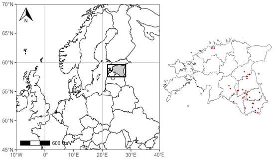
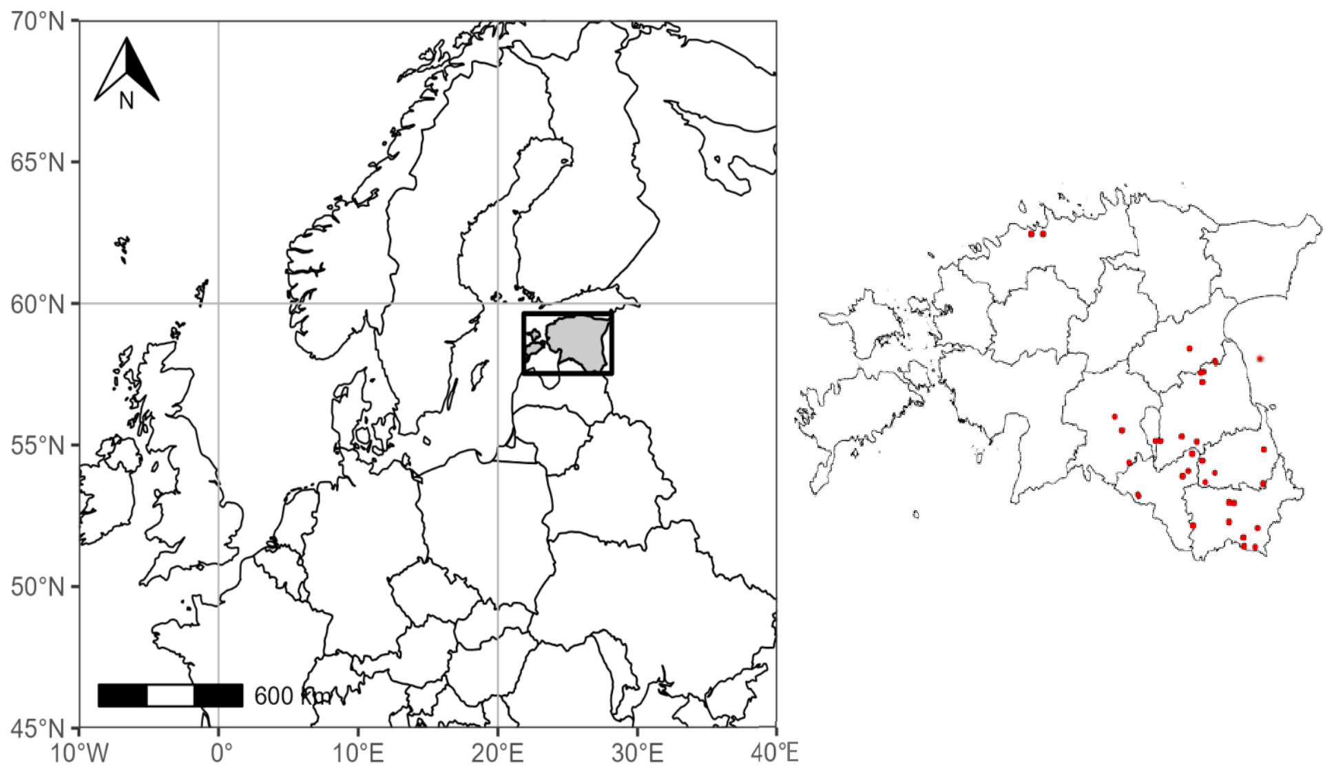
Water samples for laboratory analyses were gathered three times over the vegetation period (April–May in spring, July August in summer, and September–October in autumn) of three years (2018–2020) from various small lakes in Estonia (30 lakes in total) (Figure 1). Samples were collected from a depth of 0.5 m and stored in the dark until filtration and further analyses. For the large lakes Lake Võrtsjärv and Lake Peipsi, integrated water samples—collected from 1 m above the bottom at 0.5 m intervals and pooled together—were analysed as part of the national monitoring programme (May–October 2016–2020). Absorption parameters (phytoplankton absorption aph, absorption of non-algal particles adp) were measured according to Tassan & Ferrari [33], using NaClO as a solvent. Samples for Chl-a were extracted with 96% ethanol, measured spectrophotometrically, and calculated according to Jeffrey & Humphrey [34]. Samples for coloured dissolved organic matter (CDOM) were filtered through 0.2 µm cellulose acetate filters and measured spectrophotometrically with a Hitachi U-3010 (Hitachi Ltd., Tokyo, Japan) spectrophotometer [35]. The phytoplankton community composition, phytoplankton and cyanobacterial biomass were assessed using light microscopy [36] (Zeiss Axio Vert.A1 (Carl Zeiss, Jena, Germany)). At least 400 units were counted and converted to biovolume according to the measurements of cells, trichomes, or colonies, approximating them to simple geometric shapes [37]; biomass is reported as wet weight [38].
Figure 1.
An overview of the study area and locations of the studied lakes (red dots).
2.2. In Situ Measurements of Remote Sensing Reflectance
The water-leaving reflectance spectra were calculated from:
(1) Measurements with three above-water TriOS-RAMSES hyperspectral radiometers, following the protocol of REVAMP [39]. The calculations included the following steps: first, all measured radiance and irradiance spectra were corrected for stray light [40]; second, water-leaving reflectance ρw(λ) was calculated using remote sensing reflectance Rrs(λ) [41].
where is the upwelling radiance from the water, is the downwelling radiance from the sky, is the downwelling irradiance, and (W) is the water surface reflectance as function of wind speed W (m·s−1), calculated according to Equation (2).
Third, the Near-Infrared (NIR) similarity correction with λ1 = 720 nm, λ2 = 780 nm, and α = 2.35 was applied to the water-leaving reflectance [42,43].
(2) Measurements with two TriOS-RAMSES hyperspectral radiometers for in-water measurements. Five measurements were recorded at each depth, then Rrs(λ) was retrieved:
where Rrs(λ) is the remote sensing reflectance, Lu(λ) is the upwelling radiance from the water and Ed(λ) is the downwelling irradiance. The NIR similarity correction was again applied to the water-leaving reflectance [43].
The reason for using two methods is related to the availability of reflectance data, as for the majority of small-lake samples, reflectance data measured with a two-sensor TriOS-RAMSES system were available. We used only measurements where one sensor was placed above the water surface and the other below the surface to reduce sun-glint effects.
Based on in situ radiometric measurements, optical water types were calculated based on remote sensing reflectance spectra according to Uudeberg [44].
2.3. Satellite Data
We wanted to test an atmospheric correction processor, which is available for both S2 and S3, is applicable to all our lake types, and gives phytoplankton absorption as an output. This was the reason behind choosing C2RCC.
S2/MSI Level 1 (L1) and S3/OLCI L1 and Level 2 (L2) full-resolution (FR) non-time critical data were downloaded for the period 2016–2020:
- S2 A/B MSI data were downloaded from the Copernicus Open Access Hub (https://scihub.copernicus.eu, accessed on 10 October 2023), with processing baselines of 02.04–04.00, data now available for download from Copernicus Data Space Browser (https://browser.dataspace.copernicus.eu/, accessed on 10 October 2023).
- S3 A/B OLCI L1 data were downloaded from the EUMETSAT Data Store (https://data.eumetsat.int, accessed on 1 October 2023) for 2016–2019 (reprocessed), or from the EUMETSAT Data Centre (https://archive.eumetsat.int/, accessed on 12 October 2023) for 2020 with a processing baseline of 002, data now available for download from Copernicus Data Space Browser (https://browser.dataspace.copernicus.eu/, accessed on 12 October 2023).
L1 data for both S2 MSI and S3 OLCI were processed using C2RCC (v.2.1) [17,45] atmospheric correction. Its water part uses a neural network that estimates five inherent optical properties at 443 nm from the water-leaving reflectance spectrum [17]; here, we focused on apig. The following C2RCC flags were used for S3: Rhow_OOS, Cloud_risk, Rhow_OOR, Rtosa_OOR, quality_flags_invalid, Rtosa_OOS, and quality_flags_sun_glint_risk.
For S2 the first approach consisted of the application of commonly used C2RCC flags: Rtosa_OOS, Rtosa_OOR, Rhow_OOS, Rhow_OOR Cloud_risk, Valid_PE and IdePix (9.0.2) [46] flags: IDEPIX_VEG_RISK, IDEPIX_INVALID, IDEPIX_CLOUD, IDEPIX_CLOUD_AMBIGOUS, IDEPIX_CLOUD_SURE, IDEPIX_CLOUD_BUFFER, IDEPIX_CIRRUS_SURE, IDEPIX_CLOUD_SHADOW, IDEPIX_CIRRUS_AMBIGUOUS, IDEPIX_BRIGHT, IDEPIX_POTENTIAL_SHADOW, IDEPIX_LAND, and IDEPIX_VEG_RISK.
For the second approach, the following flags were applied in addition to those used in the first approach to ensure that values were within the neural network training range (Apig, Adet, Agelb, Bpart, Bwit_at_max; Apig, Adet, Agelb, Bpart, and Bwit at_min) and to remove datapoints outside this range. Additionally, filtering was performed based on satellite-derived uncertainty estimates for apig, removing values with uncertainty >5 m−1.
The salinity was set to 0.001 PSU, which differs from the default settings, as we were focusing on freshwater conditions. Regions of interest (ROIs) of 1 × 1 pixels, matching in situ sampling locations, were exported using the Pixel Extraction tool in Sentinel Application Platform (SNAP v9.0) software. For match-up analysis, the S3 validation protocol was followed [47] for both S2 MSI and S3 OLCI. An in situ dataset, used for validation, was collected on the same day as the satellite overpass and consisted of 109 water samples for S2 and 118 water samples for S3, including 20 water samples for S2 and 66 water samples for S3 without radiometric data or OWT classification. Satellite observations were taken on 30 different dates; however, several data points originate from the same day because fieldwork was intentionally planned during clear-sky conditions and S2 overpasses. The maximum number of small lakes visited in one day was six.
2.4. Error Metrics
Statistical analysis was performed using R software (v2025.05.1). Standard deviations for error estimation of in situ data were calculated when multiple measurements were available for one water sample or one measurement station. MDE (mean difference error) measures the average signed difference between predicted and observed values as follows:
The median absolute percentage error (MdAPE) was calculated to estimate the dispersion of the data around the 1:1 line.
R2 value (Equation (6)) indicates the fit of the model to the data; higher values represent a better fit.
Root mean square error (RMSE) was used to estimate the model error.
Normality was assessed using the Shapiro–Wilk test [48], which evaluates the null hypothesis that the data are drawn from a normally distributed population. Following best-practice guidelines, p > 0.05 was interpreted as a failure to reject normality.
2.5. Water Framework Directive Lake Types
Estonian lakes are classified according to five key parameters: water area, stratification, water colour, chloride content, and water hardness (Table 1) [49].
Table 1.
Relevant parameters for lake classification.
Based on these criteria, eight Water Framework Directive (WFD) lake types are defined (Table 2).
Table 2.
Classification of WFD lake types, based on parameter values from Table 1.
In this article, WFD lake types I and VIII were excluded, as these lakes are generally transparent with a visible bottom, and were therefore not visited during remote sensing-focused fieldwork.
3. Results
3.1. Overview of Optically Active Substances in Different Optical Water Types
General characteristics of the dataset: Chl-a ranged from 0.01 to 109.6 mg m−3 (average, 23.2 mg m−3); Secchi depth was in the range 0.1–7 m (average, 1.6 m); absorption by CDOM (aCDOM(443)) was in the range 0.7–47.3 m−1 (average, 4.1 m−1); and the amount of total suspended matter (TSM) ranged from 0.8 to 143.3 g/m3 (average, 8.4 g/m3).
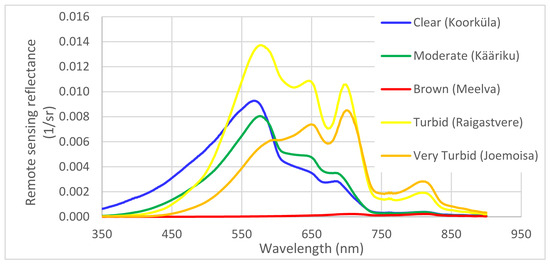
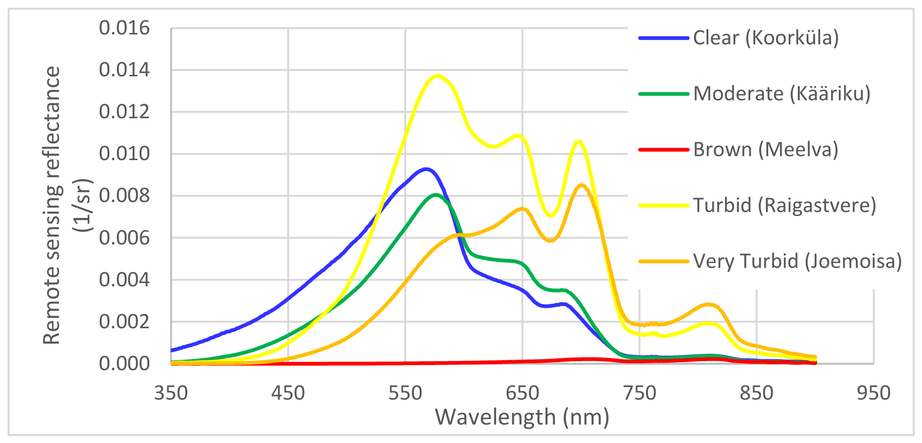
An example of various optical water types is shown in Figure 2. Clear and Moderate OWTs have maximum reflectances between 540 and 580 nm. For the Clear OWT, the reflectance at 500 nm exceeds that at 650 nm and is also higher than the reflectance at 500 nm for the Moderate OWT. The Turbid OWT has a reflectance maximum between 580 and 605 nm. The Very Turbid OWT has a reflectance maximum at wavelengths between 685 and 715 nm. The Brown OWT has a maximum in the red part of the spectrum, whereas reflectance tends to be below 0.006.
Figure 2.
An example of reflectance spectra for five different optical water types.
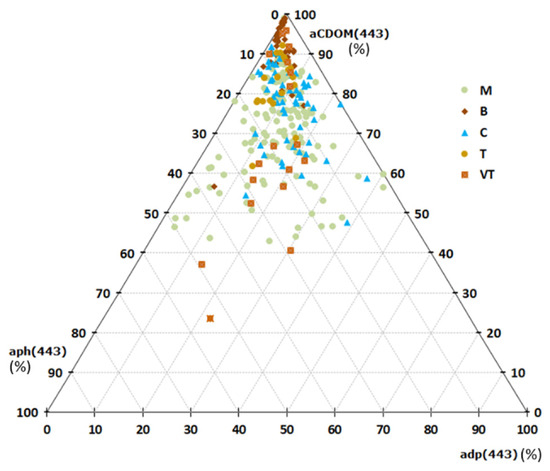
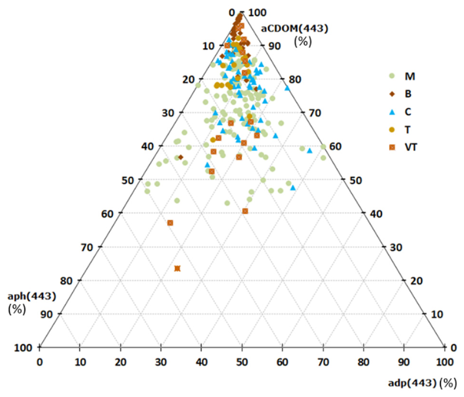
Absorption by CDOM largely determined the underwater light field (Figure 3). This effect was most pronounced in the Brown water type, where CDOM absorption accounted for nearly 100%. In the Moderate and Clear types, absorption by all components ranged from 10% to 50%, with both phytoplankton (aph) and CDOM dominating. Turbid waters exhibited high CDOM absorption, whereas Very Turbid waters showed a stronger contribution from phytoplankton (up to 55%).
Figure 3.
The share (%) of different absorbers (absorption by phytoplankton, aph; absorption by CDOM, aCDOM; and absorption by non-algal particles, adp) at 443 nm. The colours represent various OWTs (C—Clear, M—Moderate, B—Brown, T—Turbid, and VT—Very Turbid).
3.2. OWTs in Different WFD Lake Types
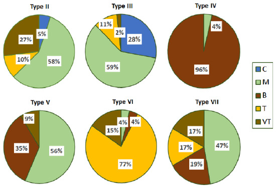
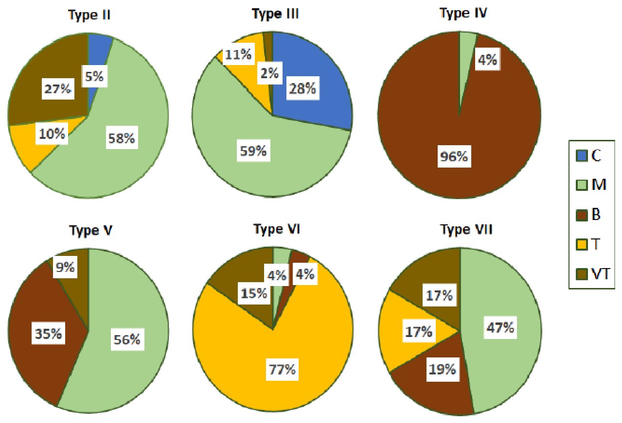
WFD classification for Estonian lakes partly relies on water colour, distinguishing highly absorbing waters (Type IV). This type corresponded well to the Brown OWT with a small share (4%) of the Moderate OWT (Figure 4). The main difference between WFD lake types II and III is the presence of summer stratification in type III. Both types had similar shares (58–59%) of the Moderate and Turbid OWTs, but Type II included a larger proportion of Very Turbid waters (27%), whereas Type III had more Clear waters (28%). Type V consists mainly of Moderate waters (56%), with Brown (35%) and a minor share of Very Turbid (9%) waters. Type VI (Lake Võrtsjärv) is predominantly Turbid (77%), occasionally Very Turbid (15%), and includes small proportions (4%) of Moderate and Brown OWTs. Type VII (Lake Peipsi) is mostly Moderate (47%), with nearly equal shares of Brown, Turbid, and Very Turbid OWTs.
Figure 4.
The share of different optical water types (C—Clear, M—Moderate, B—Brown, T—Turbid, and VT—Very Turbid) in the six lake types used for WFD reporting in Estonia.
3.3. Phytoplankton Absorption in Relation to Chlorophyll-a Concentration
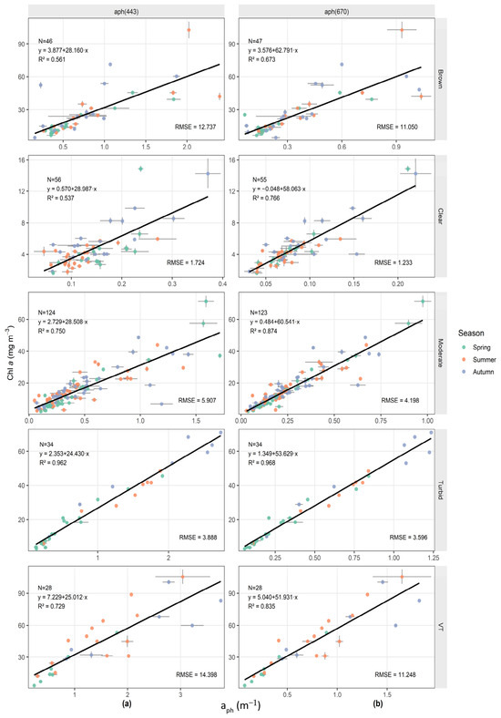
A moderate-to-strong linear relationship was observed between phytoplankton pigment absorption and Chl-a concentration (Figure 5). In the Clear OWT, Chl-a remained below 15 mg/m3, corresponding to low pigment absorption (up to 0.4 m−1). The Moderate OWT exhibited Chl-a up to 60 mg/m3, with aph(443) reaching 1.7 m−1. The Brown OWT generally had Chl-a below 80 mg/m3, except for one extreme value near 100 mg/m3 from Lake Valguta Mustjärv; most aph(443) values were below 2 m−1. The Turbid OWT reached Chl-a up to 70 mg/m3 and aph(443) up to 2.7 m−1, while the Very Turbid OWT exceeded 100 mg/m3, with aph(443) peaking at 3.8 m−1.
Figure 5.
In situ-measured phytoplankton absorption (aph) in relation to in situ-measured Chl-a amount for 5 different optical water types, (a) at 443 nm and (b) at 670 nm. Note the difference in x and y scales.
The effect of season was visible only in Turbid and Very Turbid OWTs, where the majority of spring values were lower in comparison with summer and autumn values. At the same time, in the Moderate OWT, the highest values for aph and Chl-a were found in spring. In the Clear OWT, higher values were from spring and autumn.
The linear relationship between measured aph and Chl-a was strongest in the case of the Turbid OWT (R2 = 0.96), and the weakest in the case of Clear (R2 = 0.53) and Brown OWTs (R2 = 0.56). The use of the red spectrum (670 nm) resulted in a stronger relationship between aph and Chl-a for all OWTs. RMSE for Chl-a retrieval from aph(443) was the highest in the case of Very Turbid (14.4 mg/m3) and Brown OWTs (12.7 mg/m3), and the lowest in the case of the Clear OWT (1.72 mg/m3). The RMSE was 3.89 mg/m3 for the Turbid OWT and 5.91 mg/m3 for the Moderate OWT. For all OWTs, Chl-a retrieval from aph(670) resulted in a lower RMSE.
Because the Chl-a-aph relationship differs among OWTs, model transformation was applied on OWT-specific bases. Log-scale residuals for Clear, Moderate, and Brown OWTs showed Shapiro–Wilk p-values exceeding 0.05, indicating no significant deviation from normality, supporting the use of log–log models for these optical water types. The resulting log-scale models for these three OWTs were used to model Chl-a, whereas a linear model was retained for the Turbid and Very Turbid OWTs.
Model performance is shown in Figure A1; the coefficient of determination (R2) was higher for the Turbid OWT, despite the use of log-scale models for the Clear, Brown and Moderate OWTs. However, Chl-a retrievals achieved lower MDAPEs (%) for the Clear, Brown, and Moderate OWTs—for both predictors (aph(443) and aph(670)) under the log-scale transformation—and a lower MDE when modeling from aph(670) (Appendix A, Table A1 and Table A2).
3.4. Phytoplankton Biomass and Communities in Different OWTs
Having established how phytoplankton absorption varies with Chl-a across OWTs and seasons, the next section focuses on broader ecosystem characteristics by examining phytoplankton biomass and community composition within the same OWT framework.
3.4.1. Phytoplankton and Cyanobacterial Biomass
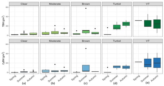
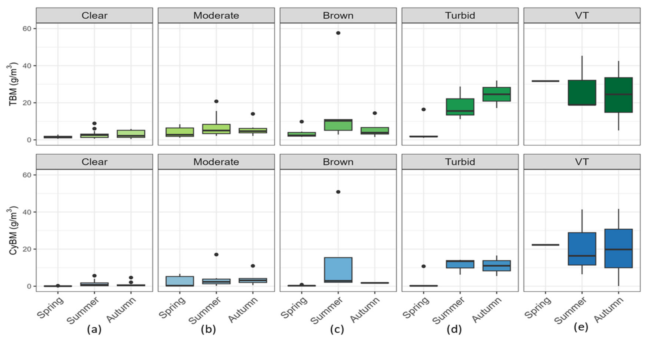
Phytoplankton total biomass and cyanobacterial biomass were the lowest in Clear OWT (<10 g/m3), with minimal variability and the lowest values in spring (Figure 6). In the Moderate OWT, biomass peaked in summer, reaching 20 g/m3. The Brown OWT generally showed lower biomass in spring and higher in summer, with occasional extreme values driven by cyanobacteria—an atypical feature caused by one lake with exceptionally high pH (>9). In the Turbid OWT, biomass was lowest in spring and increased steadily toward autumn (>30 g/m3), with cyanobacteria dominating in summer and autumn. The Very Turbid OWT exhibited high biomass already in spring due to cyanobacteria, reaching 50 g/m3 in summer, with the greatest variability during summer and autumn.
Figure 6.
Phytoplankton biomass (TBM) and cyanobacterial biomass (CyBM) based on in situ data for different OWTs. (a) Clear, (b) Moderate, (c) Brown, (d) Turbid, and (e) Very Turbid (VT).
3.4.2. Seasonal Changes in Phytoplankton Community Composition in Selected Lakes
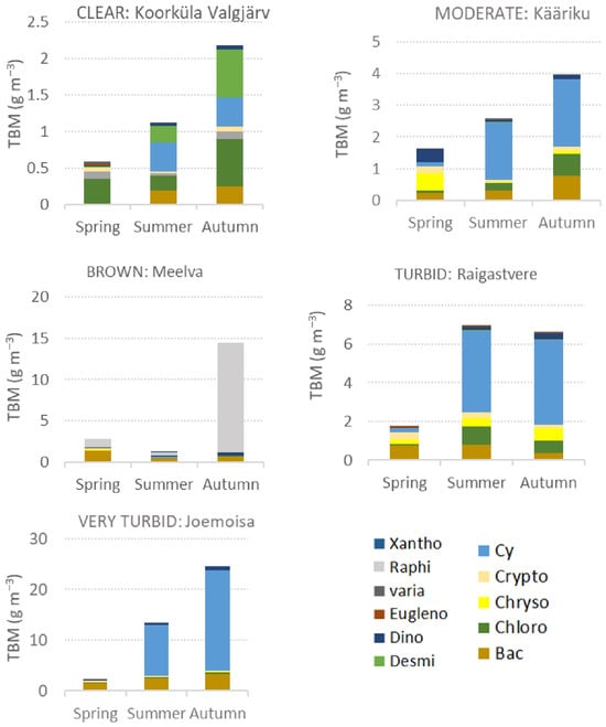
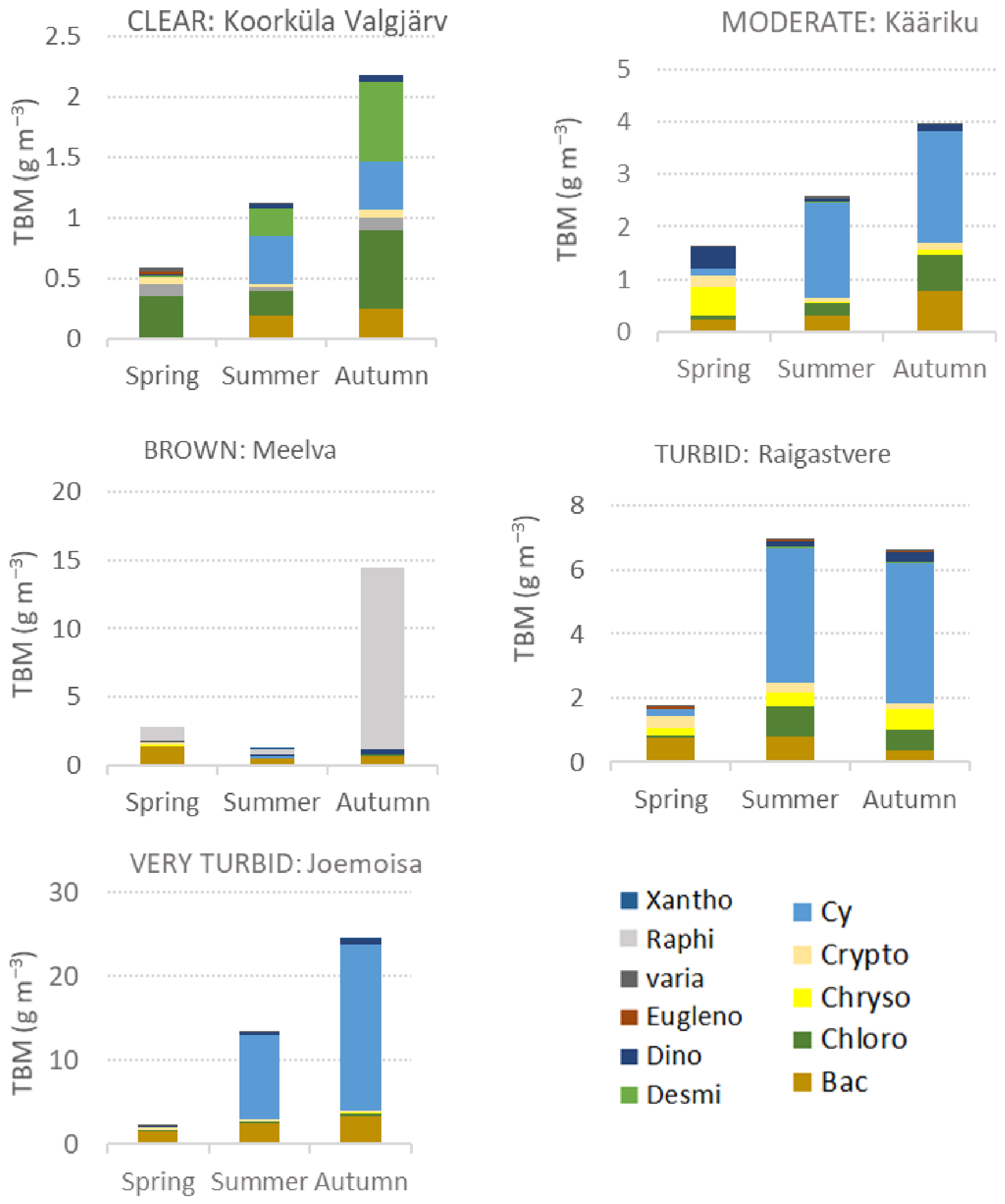
Here, an example of phytoplankton community structure across various OWTs is given. In the presented lakes, OWTs remained consistent throughout the vegetation period. Seasonal changes were present in all types of lakes. Diatoms were present in all samples except in the Clear OWT during spring (Figure 7). In the Clear OWT, phytoplankton biomass was the lowest (Figure 6), and the phytoplankton community was characterized throughout the vegetation period by chlorophytes, while cyanobacteria and Desmidiales dominated during summer and autumn (Figure 7). In all selected lakes, phytoplankton biomass was lowest in springtime, except for the Brown OWT, which had the lowest biomass in summer. The Brown OWT exhibited a peak in biomass in autumn, driven by the raphidophyte Gonyostomum semen. Phytoplankton biomass increased in selected lakes from spring to autumn in the Clear, Moderate, and especially in the Very Turbid OWT. The biomass of cyanobacteria increased from summer to autumn; their biomass increased from Clear to Moderate to Turbid OWTs, being the highest in the Very Turbid OWT. In the Turbid OWT, phytoplankton biomass was highest in summer, with clear cyanobacterial dominance.
Figure 7.
An example of seasonal dynamics of phytoplankton biomass (TBM) of various groups (Bac—diatoms, Chloro—chlorophytes, Chryso—chrysophtes, Crypto—cryptophytes, Cy—cyanobacteria, Desmi—desmidiales, Dino—dinoflagellates, Eugleno—euglenophytes, Raphi—raphidophytes, and Xantho—xanthophytes) in selected lakes belonging to different OWTs. Note the differences in the y-axes.
3.5. Satellite Retrieval of Phytoplankton Absorption and Validation
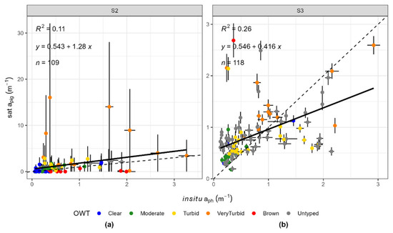
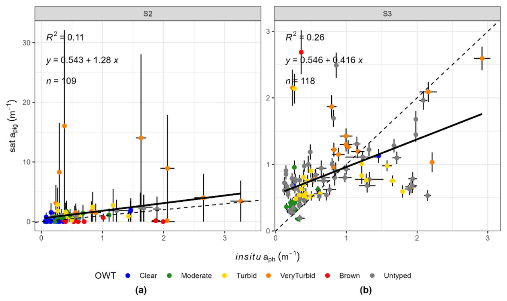
S2 initially retrieved much larger apig values (up to 16 m−1) than S3, which obtained values below 3 m−1 (Figure 8). All unrealistically large values retrieved by S2 belonged to the Very Turbid OWT and were associated with high uncertainties. Further analysis of S2 data was carried out after removing values with uncertainties exceeding 5 m−1.
Figure 8.
Phytoplankton absorption (apig) from different satellites, (a) Sentinel 2 (S2) and (b) Sentinel 3 (S3), in comparison with in situ-measured phytoplankton absorption (aph) values. Y-scale error bars denote satellite uncertainties, x error bars denote in situ variability. Colours represent various OWTs; grey is for untyped water samples lacking radiometric measurements. The dashed line is a 1:1 line. Black solid line represents a linear relationship between parameters.
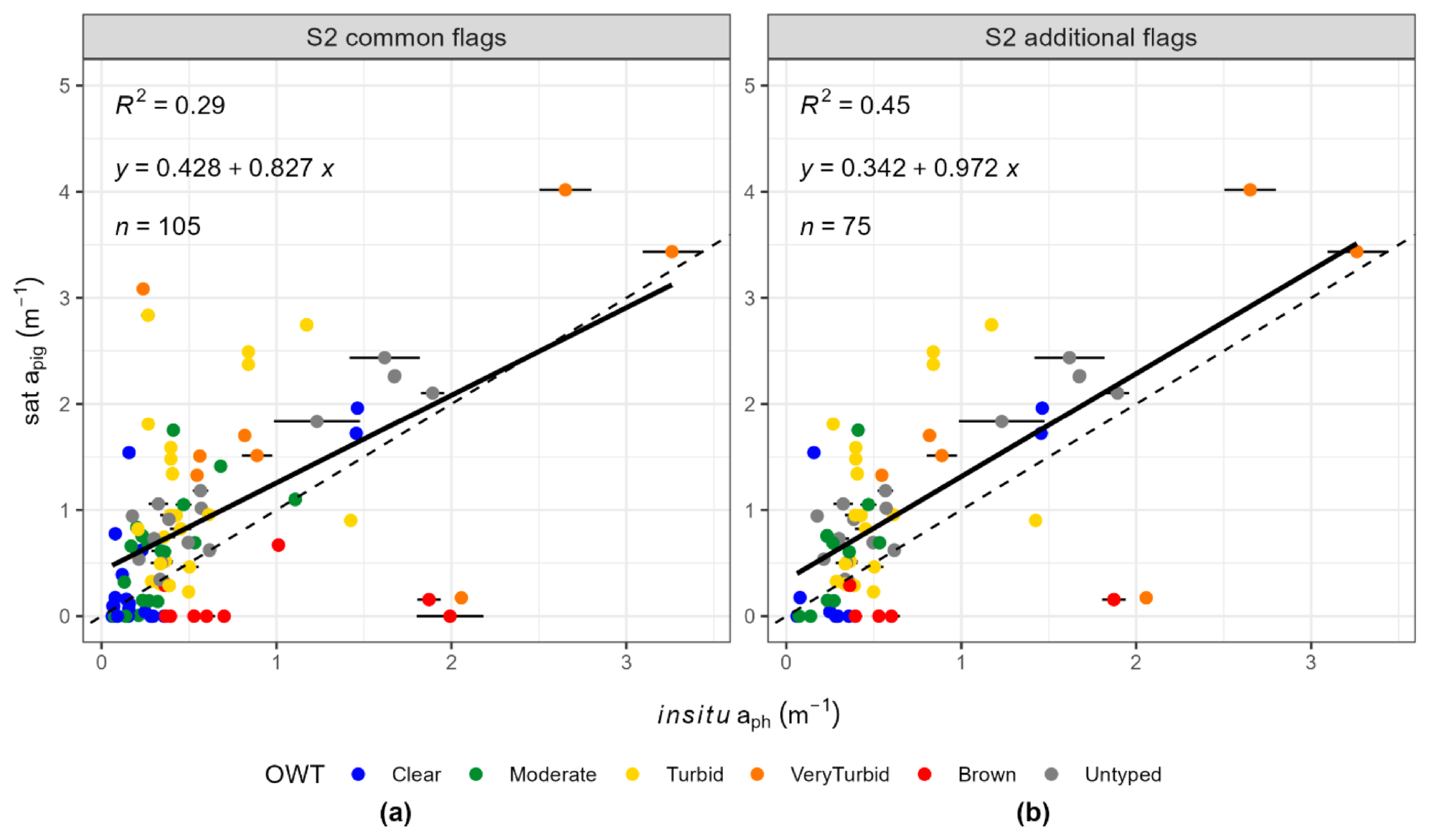
The coefficient of determination between in situ-measured aph and satellite-estimated apig was low (R2 = 0.11–0.26). After removing values with high uncertainties, this relationship increased slightly (0.29) for S2 (Figure 9), accompanied by a decrease in RMSE and MDAPE% (Table 3).
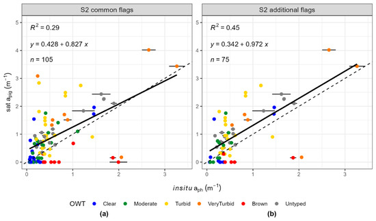
Figure 9.
Phytoplankton absorption (apig) from S2, using C2RCC. (a) Commonly used flags (approach 1); (b) commonly used flags + additional flags pertaining to training ranges in comparison with in situ-measured phytoplankton absorption values (aph). x error bars denote variability between in situ samples. Colours represent various OWTs; grey is for unclassified water samples lacking radiometric measurements. The dashed line is a 1:1 line. Black solid line represents a linear relationship between parameters.
Table 3.
Error metrics for C2RCC performance (S2 and S3). * denotes S2 data after removing values with high uncertainties (>5 m−1).
S3 tended to overestimate smaller aph values and underestimate higher ones (Figure 8b). As the dataset for S3 originated mainly from the large lakes Peipsi and Võrtsjärv, which are generally more turbid, the dataset included only one datapoint from the Brown OWT and three from the Clear OWT, specifically meaning there were no low aph values represented.
For S2, several values close to zero were observed for Clear and Brown OWTs (Figure 9). Most values from Turbid and Very Turbid OWTs were overestimated, while values from Brown and Clear OWTs were underestimated (Table 4, MDE).
Table 4.
Error metrics for apig retrieval from S2 (with commonly used flags; approach 1) and S3 data in different OWTs.
When analyzing results by OWT, MDAPE was the lowest for S3 in the Very Turbid OWT (29.8%) and higher for the Turbid (53%), Clear (56%) and Moderate (65.2%) OWTs. For S2, the Turbid OWT showed the largest dispersion in apig (>100%), while for other OWTs MDAPE% remained slightly below 100%.
Including S2 flags related to the neural network training range reduced the number of data points across all OWTs (Table 5) and increased the strength of the relationship, with R2 improving to 0.45 for the entire dataset (Figure 9b). This adjustment improved detection in the Turbid and Very Turbid OWTs (MDE decreased from 0.56 to 0.45 and from 0.83 to 0.70, respectively), along with lower RMSE. R2 for the Clear OWT increased to 0.6.
Table 5.
Error metrics for apig retrieval from S2 with all flags (approach 2) applied in different OWTs.
4. Discussion
Space-based observations of ocean colour remain the primary approach for estimating chlorophyll-a concentration in the surface layer of both oceanic and inland waters at regional-to-global scales [50,51]. Applying OWTs to reflectance spectra enables the development of OWT-specific methods for detecting in-water substances [31].
The performance of any optical model depends on the interaction between phytoplankton pigments, community composition, and background water constituents. As shown in Figure 2, the lakes examined here exhibit a high proportion of CDOM absorption, which strongly shapes the underwater light climate and strongly reduces Chl-a detection in the blue region. CDOM darkens the water and decreases the depth of the euphotic zone [52,53]. However, dark water does not necessarily indicate low Chl-a concentrations, as inputs of allochthonous organic material may increase nutrient availability and promote phytoplankton growth [53].
Retrieving accurate satellite signals from such dark waters is challenging (as also shown in Section 3.3), because most light is absorbed and only a small fraction reaches the sensor, making the instrument’s signal-to-noise ratio particularly important. This is evident in S2 retrievals (Figure 8 and Figure 9), where most Brown OWT values were retrieved as near-zero. In this OWT, strong CDOM absorption overlaps with phytoplankton pigment absorption (especially <500 nm), which makes aph(443) a less reliable predictor of Chl-a than aph(670).
In the Clear OWT, CDOM influence is low, but pigment concentrations are also low, still limiting satellite detectability. Turbid and Very Turbid OWTs have higher Chl-a concentrations and phytoplankton biomass than other OWTs, which should in principle improve retrieval performance. However, S2 retrievals for the Very Turbid OWT frequently exhibited high uncertainties, demonstrating that high biomass values alone do not guarantee reliable retrievals when factors such as high turbidity, backscattering variability and adjacency effects also affect reflectance.
We used C2RCC because it has demonstrated strong statistical performance in inland waters, alongside POLYMER, when compared to ACOLITE’s DSF mode, iCOR, L2gen, and Sen2Cor [54,55]. C2X is another processor, known to perform well in turbid and very turbid waters [56,57], but because it rejects many oligotrophic–mesotrophic pixels [56], it is not suitable for the full range of lake types considered here. C2RCC is available for both S2 and S3 and is specifically designed for Case II waters [58], making its training range suitable for boreal and temperate lakes. Yet, recent work shows that no atmospheric correction algorithm consistently outperforms others across diverse atmospheric and water conditions [14,59], highlighting the need for continual refinement of atmospheric correction schemes. Accurate atmospheric correction must also address adjacency effects, which influence all small lakes, and the RadCor processor has shown promising results [60].
A4O-ONNS represents a further development of C2RCC for S3 by incorporating OWTs [18,61]. Its performance has been tested for optically complex waters [21], and A4O-ONNS (v1.0) retrieved apig(440) with slight improvement (R2 = 0.43), but with systematic overestimation (MdPE = 72%).
The relationship between the Chl-a concentration and the phytoplankton absorption coefficient varies across optically complex inland waters [62]. The modified quasi-analytical algorithm (MQAA) applied to optically complex lake data produced a linear model for Chl-a (up to 45 mg/m3) and inversed aph(674) with R2 = 0.87, resulting in a similar R2 as linear relationship between measured Chl-a concentration and aph(674) [63]. The Chl-a retrieval uncertainties in most semi-analytical algorithms from satellite data are primarily determined by phytoplankton absorption and composition, while machine leaning algorithms show high sensitivity to CDOM and detritus absorption [64]. This again highlights the importance of in situ absorption measurements and phytoplankton community composition information.
The key limitation is evident—accurate Chl-a retrieval is only possible if apig is reliably retrieved. The C2RCC optical model for Case II waters is based on the MERIS Case II bio-optical model, which was trained using the NOMAD dataset, containing measurements from the North and Baltic Seas, and the Coastcolour dataset, representing mainly open ocean, sea, or coastal waters [65], suggesting the need for the inclusion of data from various inland waters. Because C2RCC computes Chl-a directly from apig using CHL_NN = 21 × apig1·04, even a small 0.1 increase in apig translates into a ~2 mg m−3 change in Chl-a. Our relatively weak relationships between measured and satellite-derived apig (Figure 8 and Figure 9, Table 3, Table 4 and Table 5) suggest the need for improved apig detection models. An OWT-specific approach (Figure 5) may enhance Chl-a detection, but only if apig retrieval is reliable. There is strong potential for this, as in situ data-based analysis showed an R2 up to 0.97 for Chl-a detection from aph, particularly in the Turbid OWT. A logarithmic model was more appropriate for Clear, Brown, and Moderate OWTs, resulting in lower MdAPE%, while the Turbid OWT achieved the highest accuracy (relatively low RMSE and high R2).
The selection of quality and range flags is important. Adding additional flags to S2, related to the training range of IOP parameters, reduced the number of data points and increased R2. However, S2 still produced extremely low and high apig values, which were not eliminated by flagging. Extremely large apig values originated from two lakes, Kaiu and Joemoisa, both classified into the Very Turbid OWT during summer and autumn, where high CDOM and phytoplankton biomass coexist. Figure 7 illustrates cyanobacterial dominance and high biomass in Joemoisa Lake. As these lakes are connected, phytoplankton composition is similar in both, yet measured aph values were much lower than satellite-derived values.
Lake Valguta Mustjärv (Brown OWT) is another exception among dark lakes—despite its dark water, it has a high pH and annual cyanobacterial blooms, attributed to historical nutrient additions for lawn growth in the bog during preparations for the 1980 Moscow Olympic Games [66]. Additional raphidophyte blooms were observed in several dark-water lakes, such as Lake Meelva (Figure 7) and L. Valguta Mustjärv, typically occurring during summer and autumn. In L. Meelva, these blooms were a consistent feature throughout the study period, peaking in autumn, whereas in Valguta Mustjärv a Gonyostomum bloom occurred only in 2018. In non-bloom dark lakes, raphidophytes were absent (e.g., Nohipalu Mustjärv), total biomass was much lower (around 3 g/m3), and the community was dominated by cryptophytes and desmidiales. From a satellite imaging perspective, non-bloom dark lakes are particularly challenging because CDOM masks the blue spectral region and reflectance is low [67].
Chlorophyll-a content varies across phytoplankton taxonomic groups. The carbon:chlorophyll-a (C:Chl-a) ratio differs among taxa and responds to environmental conditions [68]. Cyanobacteria typically contain more accessory pigments and less chlorophyll-a per cell or per unit biomass compared to many eukaryotic algae (e.g., diatoms, chlorophytes, or picoeukaryotes) [69,70]. As eutrophication promotes cyanobacterial dominance, and because their pigment composition enhances their success in turbid environments [71,72], this group becomes more abundant in Turbid and Very Turbid OWTs (Figure 6 and Figure 7). Diatoms on the other hand have a high amount of Chl-a per cell, but the ratios are variable, depending on the genera [70]. Large diatoms are usually dominant in moderate nutrient conditions during spring and autumn, when mixing keeps them in the water column [73].
External factors—including light availability, nutrient concentrations, and temperature—also influence chlorophyll-a content. Low-light conditions tend to increase Chl-a content, whereas nutrient limitation generally reduces it [68,74]. Consequently, this variability makes using Chl-a as a proxy for phytoplankton biomass challenging, especially across diverse waterbodies where phytoplankton communities respond differently to variations in nutrient and light regimes.
Accurate detection of Chl-a using satellite remote sensing is important for WFD reporting, as EO data may be increasingly incorporated into future reporting frameworks [75]. Our analysis revealed that only one lake type (IV) was almost entirely characterized by a single OWT (Brown), which remained seasonally stable. Other WFD types exhibited substantial variability in OWTs, with shallower types II, VI, and VII showing more turbid OWTs than type III (Figure 4). Stratification tends to result in clearer water during summer, as surface nutrients are depleted, whereas in shallow lakes, wind-induced sediment resuspension increases available phosphorus, promoting phytoplankton growth [76,77]. Here, there were lower Chl-a and aph values in the Clear OWT during summertime, and, in Turbid and Very Turbid OWTs phytoplankton biomass, Chl-a amount, and aph increased from spring to autumn.
Generally, small lakes are characterized by one dominant OWT, while large lakes may exhibit multiple OWTs simultaneously. In the selected small lakes (Figure 7), where seasonal changes in phytoplankton community composition were examined, the OWT remained stable during the vegetation period. However, this is not universal, and seasonal variability of OWTs in small lakes must also be considered.
Overall, our findings highlight that the performance of current atmospheric correction and bio-optical models is strongly affected by CDOM content, low signal-to-noise conditions, and the diverse composition of phytoplankton communities. These uncertainties are compounded by seasonal and taxonomic shifts that alter phytoplankton absorption and the relationship between biomass and Chl-a. While OWT-specific approaches offer improvements, their success depends on accurate retrieval of underlying absorption parameters.
Future advances include hyperspectral sensors such as NASA’s PACE Ocean Colour Instrument (OCI), which promise to reduce uncertainties in pigment retrievals [10,78], improve detection of phytoplankton composition, and support development of new algorithms for optically complex waters [79,80,81]. Additional targeted calibration datasets will be essential to refine bio-optical models to better represent variability within lakes.
5. Conclusions
In the lakes we studied, CDOM was the main light absorber, especially in the Brown OWT, where it accounted for up to 100% of absorption at 443 nm. Despite this, in situ Chl-a was strongly correlated with in situ aph, especially in the Turbid OWT. Linear models performed well for most OWTs and were suitable for Turbid and Very Turbid OWTs, whereas logarithmic models were more appropriate for Clear, Moderate, and Brown OWTs. This improved Chl-a modelling from in situ data and resulted in lower MdAPE%. Across all OWTs, R2 was higher and RMSE lower when using the red spectral region (670 nm). At the same time, apig detection accuracy was low when using C2RCC. The relationship between apig and aph was 0.26 for S3, based on a dataset with mostly Moderate, Turbid and Very Turbid OWTs. After removing the values retrieved with large uncertainty, the determination coefficient increased from 0.11 to 0.29 for S2, and with all flags applied, R2 improved to 0.45. S2 tends to overestimate apig in Turbid and Very Turbid OWTs and underestimate it in Clear and Brown OWTs, often producing near-zero values. OWT distribution within WFD lake types revealed more Turbid and Very Turbid OWTs in shallow, non-stratified lakes and the Clear OWT in stratified lakes. Although the bio-optical complexity of boreal lakes still poses significant challenges, improved Chl-a retrievals provide more reliable inputs for using satellite data for lake management purposes and support implementation of environmental directives.
Author Contributions
Conceptualization, K.K. and K.A.; methodology, K.K. and A.A.-T.; software, A.A.-T.; validation, K.K. and A.A.-T.; formal analysis, K.K.; investigation, K.K.; resources, K.K. and K.A.; data curation, K.K. and A.A.-T.; writing—original draft preparation, K.K.; writing—review and editing, K.A., K.K. and A.A.-T.; visualization, K.K. and A.A.-T.; supervision, K.A.; project administration, K.A. and K.K.; funding acquisition, K.K. and K.A. All authors have read and agreed to the published version of the manuscript.
Funding
This research was funded by Est-Lat Interreg Program, Project No. EE-LV00163 (NutriLoopWorks), and the Estonian Research Council, grant PRG2646 “Methods, Traceability and Validation of the In-Water Ocean Color Measurements”.
Data Availability Statement
Sentinel 2 and 3 data can be acquired freely from the EUMETSAT Data Store and Copernicus Data Space Ecosystem. The in situ data supporting the conclusions of this article will be made available by the authors on request.
Acknowledgments
We would like to acknowledge Ilmar Ansko and Martin Ligi for their valuable help during fieldwork. The ESA Copernicus program is acknowledged for satellite data. TO calibration/characterization labs (financed by ETAG project TT8 & European Regional Development Foundation project KosEST) helped with the calibration of radiometers. Chl-a data of lakes Peipsi and Võrtsjärv was received from the Centre for Limnology, and was gathered within the framework of the national monitoring program for these lakes. We want to thank four anonymous reviewers for their constructive comments and valuable feedback.
Conflicts of Interest
The authors declare no conflicts of interest. The funders had no role in the design of the study; in the collection, analyses, or interpretation of data; in the writing of the manuscript; or in the decision to publish the results.
Abbreviations
The following abbreviations are used in this manuscript:
| aCDOM | Absorption by Coloured Dissolved Organic Matter |
| aph | Phytoplankton absorption, measured in situ |
| apig | Phytoplankton absorption, retrieved by satellites |
| adg | Absorption by non-algal particles |
| Chl-a | Chlorophyll a |
| C2RCC | Case-2 Regional Coast Color |
| MdAPE | Median absolute percentage error |
| MDE | Mean difference error |
| OWT | Optical water type |
| RMSE | Root mean square error |
| Rrs | Remote sensing reflectance |
| S2 | Sentinel 2 |
| S3 | Sentinel 3 |
| WFD | Water Framework Directive |
Appendix A
Table A1.
Error metrics for linear regression model for Chl-a.
Figure A1.
Relationships between in situ-measured Chl-a and modelled Chl-a. Equations in the panels were used for modelled Chl-a calculations from aph. (a) Chl-a modelled from aph at 443 nm; (b) Chl-a modelled from aph at 670 nm. VT is Very Turbid OWT. The dashed line is a 1:1 line. Red solid line represents a linear relationship between parameters.
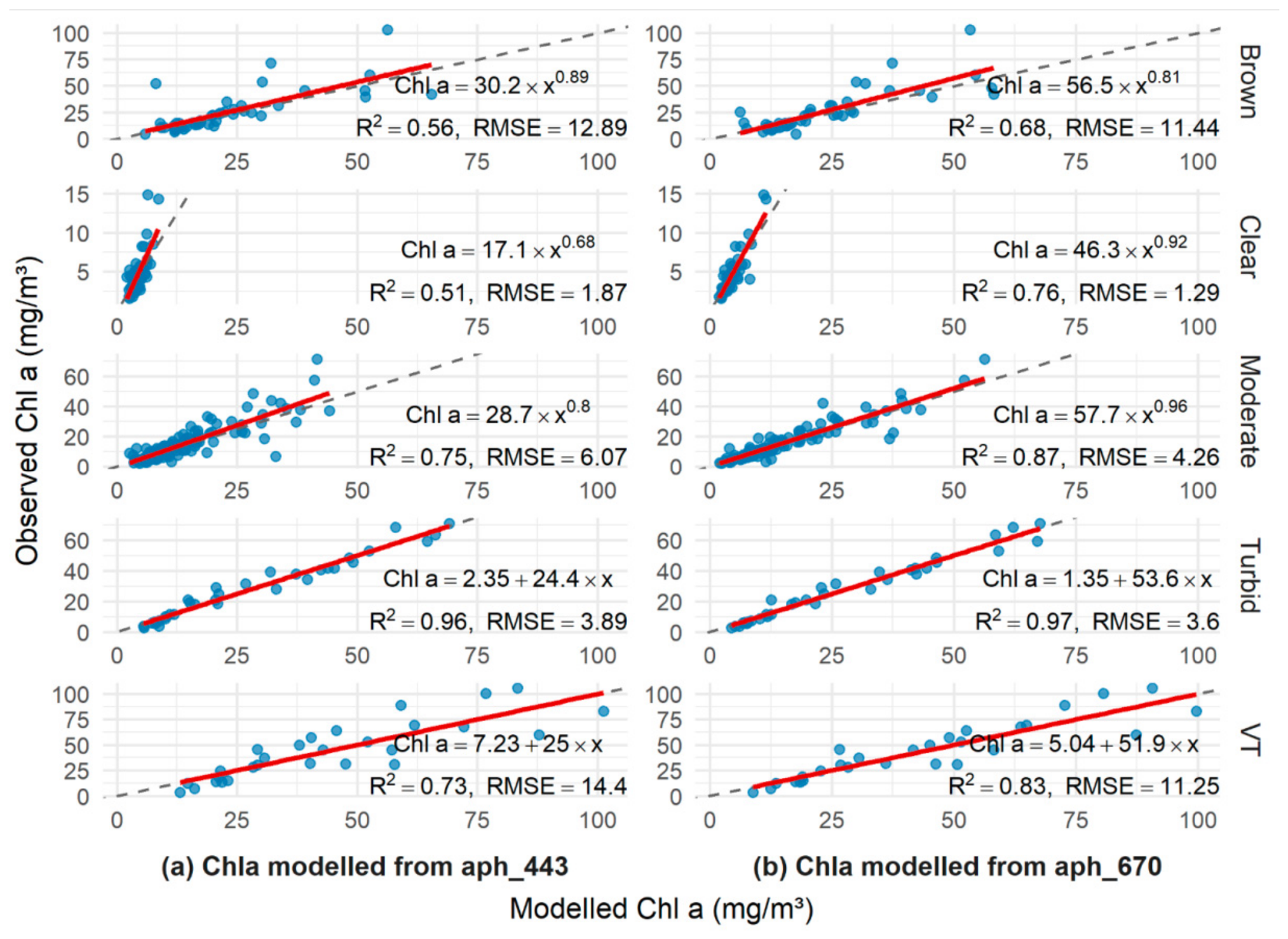
Table A2.
Error metrics for Chl-a modelled using the logarithmic model. R2-fit shows the determination coefficient of logarithmic models [82] and R2 Pred_vs_Obs shows the determination coefficient for Chl-a retrieval according to the logarithmic model.
References
- Palmer, S.C.J.; Hunter, P.D.; Lankester, T.; Hubbard, S.; Spyrakos, E.; Tyler, A.N. Validation of Envisat MERIS algorithms for chlorophyll retrieval in a large, turbid and optically-complex shallow lake. Remote Sens. Environ. 2015, 157, 158–169. [Google Scholar] [CrossRef] [Scilit]
- Neil, C.; Spyrakos, E.; Hunter, P.D.; Tyler, A.N. A global approach for chlorophyll-a retrieval across optically complex inland waters based on optical water types. Remote Sens. Environ. 2019, 229, 159–178. [Google Scholar] [CrossRef] [Scilit]
- Wei, J.; Wang, M.; Mikelsons, K.; Jiang, L. Chlorophyll-Specific Absorption Coefficient of Phytoplankton in World Oceans: Seasonal and Regional Variability. Remote Sens. 2023, 15, 2423. [Google Scholar] [CrossRef] [Scilit]
- Lyche-Solheim, A.; Feld, C.K.; Birk, S.; Phillips, G.; Carvalho, L.; Morabito, G.; Mische, U.; Willby, N.; Søndergaard, M.; Hellsten, S.; et al. Ecological status assessment of European lakes: A comparison of metrics for phytoplankton, macrophytes, benthic invertebrates and fish. Hydrobiologia 2013, 704, 57–74. [Google Scholar] [CrossRef] [Scilit]
- Pasztaleniec, A. Phytoplankton in the ecological status assessment of European lakes—Advantages and constraints. Environ. Prot. Nat. Res. 2016, 27, 26–36. [Google Scholar] [CrossRef] [Scilit]
- Alikas, K.; Kangro, K.; Reinart, A. Detecting cyanobacterial blooms in large North European lakes using the maximum chlorophyll index. Oceanologia 2010, 52, 237–257. [Google Scholar] [CrossRef] [Scilit]
- Batina, A.; Krtalić, A. Integrating Remote Sensing Methods for Monitoring Lake Water Quality: A Comprehensive Review. Hydrology 2024, 11, 92. [Google Scholar] [CrossRef] [Scilit]
- Atton Beckmann, D.; Spyrakos, E.; Hunter, P.; Jones, I.D. Widespread phytoplankton monitoring in small lakes: A case study comparing satellite imagery from Planet SuperDoves and ESA Sentinel-2. Front. Remote Sens. 2025, 6, 1549119. [Google Scholar] [CrossRef] [Scilit]
- O’Shea, R.E.; Pahlevan, N.; Smith, B.; Bresciani, M.; Egerton, T.; Giardino, C.; Li, L.; Moore, T.; Ruiz-Verdu, A.; Ruberg, S.; et al. Advancing cyanobacteria biomass estimation from hyperspectral observations: Demonstrations with HICO and PRISMA imagery. Remote Sens. Environ. 2021, 266, 112693. [Google Scholar] [CrossRef] [Scilit]
- Cetinić, I.; Rousseaux, C.S.; Carroll, I.T.; Chase, A.P.; Kramer, S.J.; Werdell, P.J.; Siegel, D.A.; Dierssen, H.M.; Catlett, D.; Neeley, A.; et al. Phytoplankton composition from sPACE: Requirements, opportunities, and challenges. Remote Sens. Environ. 2024, 302, 113964. [Google Scholar] [CrossRef] [Scilit]
- Available online: https://www.esa.int/Applications/Observing_the_Earth/Copernicus/The_Sentinel_missions (accessed on 8 December 2025).
- Available online: https://www.esa.int/Applications/Observing_the_Earth/Copernicus/Sentinel-3 (accessed on 8 December 2025).
- Available online: https://www.esa.int/Applications/Observing_the_Earth/Copernicus/Sentinel-2 (accessed on 8 December 2025).
- Pahlevan, N.; Mangin, A.; Balasubramanian, S.V.; Smith, B.; Alikas, K.; Arai, K.; Barbosa, C.; Belanger, S.; Binding, C.; Bresciani, M.; et al. ACIX-Aqua: A global assessment of atmospheric correction methods for Landsat-8 and Sentinel-2 over lakes, rivers, and coastal waters. Remote Sens. Environ. 2021, 258, 112366. [Google Scholar] [CrossRef] [Scilit]
- Li, W.; Huang, Y.; Shen, Q.; Yao, Y.; Xu, W.; Shi, J.; Zhou, Y.; Li, J.; Zhang, Y.; Gao, H. Assessment of Seven Atmospheric Correction Processors for the Sentinel-2 Multi-Spectral Imager over Lakes in Qinghai Province. Remote Sens. 2023, 15, 5370. [Google Scholar] [CrossRef] [Scilit]
- Hu, Y.; Zhan, H.; He, Q.; Zhan, W. Assessment of Atmospheric Correction Algorithms for Landsat-8/9 Operational Land Imager over Inland and Coastal Waters. Remote Sens. 2025, 17, 3055. [Google Scholar] [CrossRef] [Scilit]
- Brockmann, C.; Doerffer, R.; Peters, M.; Kerstin, S.; Embacher, S.; Ruescas, A. Evolution of the C2RCC neural network for Sentinel 2 and 3 for the retrieval of ocean colour products in normal and extreme optically complex waters. Living Planet Symp. 2016, 740, 54. [Google Scholar]
- Hieronymi, M.; Müller, D.; Doerffer, R. The OLCI neural network swarm (ONNS): A bio-geo-optical algorithm for open ocean and coastal waters. Front. Mar. Sci. 2017, 4, 140. [Google Scholar] [CrossRef] [Scilit]
- Steinmetz, F.; Deschamps, P.-Y.; Ramon, D. Atmospheric correction in presence of sun glint: Application to MERIS. Opt. Express 2011, 19, 9783. [Google Scholar] [CrossRef] [Scilit]
- Vanhellemont, Q.; Ruddick, K. Atmospheric correction of metre-scale optical satellite data for inland and coastal water applications. Remote Sens. Environ. 2018, 216, 586–597. [Google Scholar] [CrossRef] [Scilit]
- Ansper-Toomsalu, A.; Uusõue, M.; Kangro, K.; Hieronymi, M.; Alikas, K. Suitability of different in-water algorithms for eutrophic and absorbing waters applied to Sentinel-2 MSI and Sentinel-3 OLCI data. Front. Remote Sens. 2024, 5, 1423332. [Google Scholar] [CrossRef] [Scilit]
- Williamson, C.A.; Hollins, R.C. Depth profiles of Jerlov water types. Limnol. Oceanogr. Lett. 2023, 8, 781–788. [Google Scholar] [CrossRef] [Scilit]
- Jerlov, N.G. Optical studies of ocean water. In Reports of the Swedish Deep-Sea Expedition 1947–1948; 3 Physics and Chemistry, No.1; Göteborgs Kungl: Västra Frölunda, Sweden, 1951. [Google Scholar]
- Morel, A.; Prieur, L. Analysis of variations in ocean color. Limnol. Oceanogr. 1977, 22, 709–722. [Google Scholar] [CrossRef] [Scilit]
- Moore, T.S.; Campbell, J.W.; Dowell, M.D. A class-based approach to characterizing and mapping the uncertainty of the MODIS ocean chlorophyll product. Remote Sens. Environ. 2009, 113, 2424–2430. [Google Scholar] [CrossRef] [Scilit]
- Eleveld, M.A.; Ruescas, A.B.; Hommersom, A.; Moore, T.S.; Peters, S.W.M.; Brockmann, C. An optical classification tool for global lake waters. Remote Sens. 2017, 9, 420. [Google Scholar] [CrossRef] [Scilit]
- Jackson, T.; Sathyendranath, S.; Mélin, F. An improved optical classification scheme for the Ocean Colour Essential Climate Variable and its applications. Remote Sens. Environ. 2017, 203, 152–161. [Google Scholar] [CrossRef] [Scilit]
- Bi, S.; Hieronymi, M. Holistic optical water type classification for ocean, coastal, and inland waters. Limnol. Oceanogr. 2024, 69, 1547–1561. [Google Scholar] [CrossRef] [Scilit]
- Spyrakos, E.; O’Donnell, R.; Hunter, P.D.; Miller, C.; Scott, M.; Simis, S.G.; Claire, N.; Barbosa, C.F.; Binding, C.E.; Bradt, S.; et al. Optical types of inland and coastal waters. Limnol. Oceanogr. 2018, 63, 846–870. [Google Scholar] [CrossRef] [Scilit]
- Arst, H.; Reinart, A. Application of optical classifications to North European lakes. Aquat. Ecol. 2009, 43, 789–801. [Google Scholar] [CrossRef] [Scilit]
- Uudeberg, K.; Aavaste, A.; Kõks, K.-L.; Ansper, A.; Uusõue, M.; Kangro, K.; Ansko, I.; Ligi, M.; Toming, K.; Reinart, A. Optical Water Type Guided Approach to Estimate Optical Water Quality Parameters. Remote Sens. 2020, 12, 931. [Google Scholar] [CrossRef] [Scilit]
- Liu, X.; Steele, C.; Simis, S.; Warren, M.; Tyler, A.; Spyrakos, E.; Selmes, N.; Hunter, P. Retrieval of chlorophyll-a concentration and associated product uncertainty in optically diverse lakes and reservoirs. Remote Sens. Environ. 2021, 267, 112710. [Google Scholar] [CrossRef] [Scilit]
- Tassan, S.; Ferrari, G.M. An alternative approach to absorption measurements of aquatic particles retained on filters. Limnol. Oceanogr. 1995, 40, 1358–1368. [Google Scholar] [CrossRef] [Scilit]
- Jeffrey, S.W.; Humphrey, G.F. New spectrophotometric equations for determining chlorophylls a, b, c1 and c2 in higher plants, algae and natural phytoplankton. Biochem. Physiol. Pflanz. 1975, 167, 191–194. [Google Scholar] [CrossRef] [Scilit]
- Sipelgas, L.; Arst, H.; Kallio, K.; Erm, A.; Oja, P.; Soomere, T. Optical Properties of Dissolved Organic Matter in Finnish and Estonian Lake. Nord. Hydrol. 2003, 34, 361–386. [Google Scholar] [CrossRef] [Scilit]
- Utermöhl, H. Zur Vervollkomnung der quantitativen Phytoplankton-Methodik. Mitteilungen Int. Ver. Theor. Angew. Limnol. 1958, 9, 1–38. [Google Scholar]
- Wetzel, R.G.; Likens, G.E. Limnological Analyses; Springer: New York, NY, USA, 1991; 391p. [Google Scholar]
- Tikkanen, T. Kasviplanktonopas; Suomen Luonnosuojelun Tuki OY: Helsinki, Finland, 1986; 286p. [Google Scholar]
- Tilstone, G.H.; Moore, G.F.; Doerffer, R.; Røttgers, R.; Ruddick, K.G.; Pasterkamp, R.; Jørgensen, P.V. Regional Validation of MERIS Chlorophyll products in North Sea REVAMP Protocols Regional Validation of MERIS Chlorophyll products. In Proceedings of the Working Meeting on MERIS and AATSR Calibration and Geophysical Validation (ENVISAT MAVT-2003), Frascati, Italy, 20–24 October 2003. [Google Scholar]
- Vabson, V.; Kuusk, J.; Ansko, I.; Vendt, R.; Alikas, K.; Ruddick, K.; Ansper, A.; Bresciani, M.; Burmester, H.; Costa, M.; et al. Laboratory Intercomparison of Radiometers Used for Satellite Validation in the 400–900 nm Range. Remote Sens. 2019, 11, 1101. [Google Scholar] [CrossRef] [Scilit]
- Mobley, C.D. (Ed.) The Oceanic Optics Book; International Ocean Colour Coordinating Group (IOCCG): Dartmouth, NS, Canada, 2022; 924p. [Google Scholar] [CrossRef]
- Ruddick, V.; De Cauwer, V.; Van Mol, B. Use of the near infrared similarity reflectance spectrum for the quality control of remote sensing data. Remote Sens. Coast. Ocean. Environ. 2005, 5885, 588501. [Google Scholar] [CrossRef] [Scilit]
- Ruddick, K.; De Cauwer, V.; Park, Y.; Moore, G. Seaborne measurements of near infrared water-leaving reflectance: The similarity spectrum for turbid waters. Limnol. Oceanogr. 2006, 51, 1167–1179. [Google Scholar] [CrossRef] [Scilit]
- Uudeberg, K. Optical Water Type Guided Approach to Estimate Water Quality in Inland and Coastal Waters. PhD Thesis, Universitatis Tartuensis, Tartu, Estonia, 2020. Volume 124. 67p. Available online: https://dspace.ut.ee/items/d6f72f19-7c9c-492d-a8cc-b22db1a43f62 (accessed on 10 December 2025).
- Doerffer, R.; Schiller, H. The MERIS case 2 water algorithm. Int. J. Remote Sens. 2007, 28, 517–535. [Google Scholar] [CrossRef] [Scilit]
- Wevers, J.; Müller, D.; Scholze, J.; Kirches, G.; Quast, R.; Brockmann, C. IdePix for Sentinel-2 MSI Algorithm Theoretical Basis Document 2021. Available online: https://zenodo.org/record/5788067 (accessed on 7 August 2025).
- EUMETSAT. Recommendations for Sentinel-3 OLCI Ocean Colour Product Validations in Comparison with In Situ Measurements—Matchup Protocols; EUMETSAT: Darmstadt, Germany, 2021; 12p, Available online: https://user.eumetsat.int/s3/eup-strapi-media/Recommendations_for_Sentinel_3_OLCI_Ocean_Colour_product_validations_in_comparison_with_in_situ_measurements_Matchup_Protocols_V8_B_e6c62ce677.pdf (accessed on 14 September 2025).
- Shapiro, S.S.; Wilk, M.B. An analysis of variance test for normality (complete samples). Biometrika 1965, 52, 591–611. [Google Scholar] [CrossRef] [Scilit]
- Keskkonnaministri. Pinnaveekogumite Moodustamise Kord ja Nende Pinnaveekogumite Nimestik, Mille Seisundiklass Tuleb Määrata, Pinnaveekogumite Seisundiklassid ja Seisundiklassidele Vastavad Kvaliteedinäitajate Väärtused Ning Seisundiklasside Määramise Kord; Keskkonnaministri: Tallinn, Estonia, 2009; Available online: https://www.riigiteataja.ee/akt/122022019062 (accessed on 5 May 2025). (In Estonian)
- Gitelson, A.A.; Dall’Olmo, G.; Moses, W.; Rundquist, D.C.; Barrow, T.; Fisher, T.R.; Gurlin, D.; Holz, J. A simple semi-analytical model for remote estimation of chlorophyll-a in turbid waters: Validation. Remote Sens. Environ. 2008, 112, 3582–3593. [Google Scholar] [CrossRef] [Scilit]
- Arteaga, L.A.; Rousseaux, C.S. Evaluation of Vertical Patterns in Chlorophyll-A Derived from a Data Assimilating Model of Satellite-Based Ocean Color. Earth Space Sci. 2024, 11, e2023EA003378. [Google Scholar] [CrossRef] [Scilit]
- Ylöstalo, P.; Kallio, K.; Seppälä, J. Absorption properties of in-water constituents and their variation among various lake types in the boreal region. Remote Sens. Environ. 2014, 148, 190–205. [Google Scholar] [CrossRef] [Scilit]
- Ahonen, S.A.; Vuorio, K.M.; Jones, R.I.; Hämäläinen, H.; Rantamo, K.; Tiirola, M.; Vähätalo, A.V. Assessing and predicting the influence of chromophoric dissolved organic matter on light absorption by phytoplankton in boreal lakes. Limnol. Oceanogr. 2024, 69, 422–433. [Google Scholar] [CrossRef] [Scilit]
- Pereira-Sandoval, M.; Ruescas, A.; Urrego, P.; Ruiz-Verdú, A.; Delegido, J.; Tenjo, C.; Soria-Perpinyà, X.; Vicente, E.; Soria, J.; Moreno, J. Evaluation of Atmospheric Correction Algorithms over Spanish Inland Waters for Sentinel-2 Multi Spectral Imagery Data. Remote Sens. 2019, 11, 1469. [Google Scholar] [CrossRef] [Scilit]
- Warren, M.A.; Simis, S.G.H.; Martinez-Vicente, V.; Poser, K.; Bresciani, M.; Alikas, K.; Spyrakos, E.; Giardino, C.; Ansper, A. Assessment of Atmospheric Correction Algorithms for the Sentinel-2A MultiSpectral Imager over Coastal and Inland Waters. Remote Sens. Environ. 2019, 225, 267–289. [Google Scholar] [CrossRef] [Scilit]
- Soriano-González, J.; Urrego, E.P.; Sòria-Perpinyà, X.; Angelats, E.; Alcaraz, C.; Delegido, J.; Ruíz-Verdú, A.; Tenjo, C.; Vicente, E.; Moreno, J. Towards the Combination of C2RCC Processors for Improving Water Quality Retrieval in Inland and Coastal Areas. Remote Sens. 2022, 14, 1124. [Google Scholar] [CrossRef] [Scilit]
- Li, W.; Zhou, Y.; Yang, F.; Liu, H.; Yang, X.; Fu, C.; He, B. Using C2X to Explore the Uncertainty of In Situ Chlorophyll-a and Improve the Accuracy of Inversion Models. Sustainability 2023, 15, 9516. [Google Scholar] [CrossRef] [Scilit]
- C2RCC, Community Project. Available online: https://c2rcc.org/documentation/ (accessed on 23 December 2025).
- Ansari, M.; Knudby, A.; Amani, M.; Sawada, M. Retrieving Inland Water Quality Parameters via Satellite Remote Sensing: Sensor Evaluation, Atmospheric Correction, and Machine Learning Approaches. Remote Sens. 2025, 17, 1734. [Google Scholar] [CrossRef] [Scilit]
- Castagna, A.; Vanhellemont, Q. A generalized physics-based correction for adjacency effects. Appl. Opt. 2025, 64, 2719–2743. [Google Scholar] [CrossRef] [Scilit]
- Hieronymi, M.; Behr, D.; Bi, S.; Röttgers, R. Optical complexity of North Sea, Baltic Sea, and adjacent coastal and inland waters derived from Sentinel-3 OLCI satellite data. Earth Syst. Sci. Data 2026, 18, 1307–1329. [Google Scholar] [CrossRef] [Scilit]
- Sun, D.; Li, Y.; Wang, Q.; Le, C.; Lv, H.; Huang, C.; Gong, S. Specific inherent optical quantities of complex turbid inland waters, from the perspective of water classification. Photochem. Photobiol. Sci. 2012, 11, 1299–1312. [Google Scholar] [CrossRef] [Scilit]
- Zhao, L.; Huajie, D.; Daqing, W.; Jianwu, C.; Guoli, D.; Zhengdong, D.; Guangyuan, W.; Haoli, X.; Xiaoning, Z.; Yue, S. Chlorophyll-a concentration inversion based on the modified Quasi-Analytical Algorithm and Sentinel-3 OLCI in Daihai Lake, China Open Access. Water Supply 2022, 22, 2959–2976. [Google Scholar] [CrossRef] [Scilit]
- Werther, M.; Odermatt, D.; Simis, S.G.H.; Gurlin, D.; Schaffer, D.; Jorge, F.; Loisel, H.; Hunter, P.D.; Tyler, A.N.; Spyrakos, E. Characterising retrieval uncertainty of chlorophyll-a algorithms in oligotrophic and mesotrophic lakes and reservoirs. ISPRS J. Photogram. Remote Sens. 2022, 190, 279–300. [Google Scholar] [CrossRef] [Scilit]
- Doerffer, R. Algorithm Theoretical Bases Document (ATBD) for L2 Processing of MERIS Data of Case 2 Waters, 4th Reprocessing; Brockmann Consult: Hamburg, Germany, 2015; 55p, Available online: https://earth.esa.int/eogateway/documents/20142/37627/MERIS_ATBD_2.12_v2+-+2015+-+Case2_waters.pdf/1221f28b-59e7-a533-1d2a-692cb7323dd4 (accessed on 12 December 2025).
- Ott, I. Pinnavee Seisundi Hindamine, Võrdlusveekogumid ja Pinnavee Seisundi Klassipiirid Bioloogiliste Kvaliteedielementide Järgi; Eesti Maaülikool: Rannu, Estonia, 2010; 222p, Available online: https://kliimaministeerium.ee/sites/default/files/documents/2021-12/Pinnavee%20seisundi%20hindamine%2C%20v%C3%B5rdlusveekogumid%20ja%20pinnavee%20seisundi%20klassipiirid%20bioloogiliste%20kvaliteedielementide%20j%C3%A4rgi.pdf (accessed on 12 December 2025). (In Estonian)
- Kutser, T.; Paavel, B.; Verpoorter, C.; Ligi, M.; Soomets, T.; Toming, K.; Casal, G. Remote Sensing of Black Lakes and Using 810 nm Reflectance Peak for Retrieving Water Quality Parameters of Optically Complex Waters. Remote Sens. 2016, 8, 497. [Google Scholar] [CrossRef] [Scilit]
- Gui, J.; Sun, J. Phytoplankton carbon to chlorophyll a model development: A review. Front. Mar. Sci. 2024, 11, 1466072. [Google Scholar] [CrossRef] [Scilit]
- Reynolds, C.S. Ecology of Phytoplankton; Cambridge University Press: Cambridge, UK, 2006; 535p. [Google Scholar]
- Yacobi, Y.Z.; Zohary, T. Carbon:chlorophyll a ratio, assimilation numbers and turnover times of Lake Kinneret phytoplankton. Hydrobiologia 2010, 639, 185–196. [Google Scholar] [CrossRef] [Scilit]
- Nõges, P.; Mischke, U.; Laugaste, R.; Solimini, A.G. Analysis of changes over 44 years in the phytoplankton of Lake Võrtsjärv (Estonia): The effect of nutrients, climate and the investigator on phytoplankton-based water quality indices. Hydrobiologia 2010, 646, 33–48. [Google Scholar] [CrossRef] [Scilit]
- Gameiro, C.; Zwolinski, J.; Brotas, V. Light control on phytoplankton production in a shallow and turbid estuarine system. Hydrobiologia 2011, 669, 249–263. [Google Scholar] [CrossRef] [Scilit]
- Ptacnik, R.; Lepisto, L.; Willen, E.; Brettum, P.; Andersen, T.; Rekolainen, S.; Solheim, A.L.; Carvalho, L. Quantitative responses of lake phytoplankton to eutrophication in Northern Europe. Aquat. Ecol. 2008, 42, 227–236. [Google Scholar] [CrossRef] [Scilit]
- Begouen Demeaux, C.; Boss, E.; Graff, J.R.; Behrenfeld, M.J.; Westberry, T.K. Phytoplanktonic Photoacclimation under clouds. Geophys. Res. Lett. 2025, 52, e2024GL112274. [Google Scholar] [CrossRef] [Scilit]
- Attila, J.; Varkitzi, I.; Alikas, K.; Poikane, S.; Free, G.; Cazzaniga, I.; van de Bund, W. Use of Earth Observation Tools in Support of the WFD—State of Play for Ecological Status Monitoring and Assessment in Surface Waters of Europe; Publications Office of the European Union: Luxembourg, 2025. [Google Scholar] [CrossRef]
- Tammeorg, O.; Horppila, J.; Laugaste, R.; Haldna, M.; Niemistö, J. Importance of diffusion and resuspension for phosphorus cycling during the growing season in large, shallow lake Peipsi. Hydrobiologia 2015, 760, 133–144. [Google Scholar] [CrossRef] [Scilit]
- Zhao, S.; Hermans, M.; Niemistö, J.; Vesterinen, J.; Jilbert, T. Stratification controls the magnitude of in-lake phosphorus cycling: Insights from a morphologically complex eutrophic lake. Hydrobiologia 2025, 852, 359–376. [Google Scholar] [CrossRef] [Scilit]
- Dierssen, H.M.; Gierach, M.; Guild, L.S.; Mannino, A.; Salisbury, J.; Schollaert Uz, S.; Scott, J.; Townsend, P.A.; Turpie, K.; Tzortziou, M.; et al. Synergies between NASA’s hyperspectral aquatic missions PACE, GLIMR, and SBG: Opportunities for new science and applications. J. Geophys. Res. Biogeosciences 2023, 128, e2023JG007574. [Google Scholar] [CrossRef] [Scilit]
- Lavigne, H.; Ruddick, K.; Vanhellemont, Q. Monitoring of high biomass Phaeocystis globosa blooms in the Southern North Sea by in situ and future spaceborne hyperspectral radiometry. Remote Sens. Environ. 2022, 282, 113270. [Google Scholar] [CrossRef] [Scilit]
- Kramer, S.; Maritorena, S.; Cetinić, I.; Werdell, P.J.; Siegel, D. Phytoplankton communities quantified from hyperspectral ocean reflectance correspond to pigment-based communities. Opt. Express 2024, 32, 34482–34491. [Google Scholar] [CrossRef] [Scilit]
- Wang, W.; Liu, B.; Gao, S.; Li, J.; Zhou, Y.; Zhang, S.; Ding, Z. PhA-MOE: Enhancing Hyperspectral Retrievals for Phytoplankton Absorption Using Mixture-of-Experts. Remote Sens. 2025, 17, 2103. [Google Scholar] [CrossRef] [Scilit]
- Nakagawa, S.; Johnson, P.C.D.; Schielzeth, H. The coefficient of determination R2 and intra-class correlation coefficient from generalized linear mixed-effects models revisited and expanded. J. R. Soc. Interface 2017, 14, 20170213. [Google Scholar] [CrossRef] [Scilit] [PubMed]

Disclaimer/Publisher’s Note: The statements, opinions and data contained in all publications are solely those of the individual author(s) and contributor(s) and not of MDPI and/or the editor(s). MDPI and/or the editor(s) disclaim responsibility for any injury to people or property resulting from any ideas, methods, instructions or products referred to in the content. |
© 2026 by the authors. Licensee MDPI, Basel, Switzerland. This article is an open access article distributed under the terms and conditions of the Creative Commons Attribution (CC BY) license.