


Highlights
What are the main findings?
- AdaProtoNet combines ResNet10 and AdaLoss to achieve superior accuracy in noisy few-shot ISAR classification.
- A new large-scale dataset validates that Adaptive Relaxation outperforms traditional hard-mining strategies.
What are the implications of the main findings?
- Adaptive relaxation effectively handles ambiguous radar samples, offering a better alternative to large-margin enforcement.
- The method enhances generalization in data-limited scenarios, supporting reliable maritime and aerospace surveillance.
Abstract
Inverse synthetic aperture radar (ISAR) image classification plays a crucial role in remote sensing, traffic monitoring, and maritime surveillance. However, existing methods often suffer from limited labeled data, degraded image quality, and the insufficient adaptability of conventional loss functions. To address these issues, this paper proposes AdaProtoNet, a few-shot ISAR image classification framework based on a ResNet10 backbone and a combined adaptive and cross-entropy loss function. The model adopts a Prototypical Network architecture that balances feature extraction and class discrimination. A customized multicategory ISAR dataset is constructed through 3D target modeling and simulated radar imaging to support few-shot learning. Within the meta-learning paradigm, AdaProtoNet generates class prototypes by averaging support features and performs classification via Euclidean distance measurement. Experimental results demonstrate that AdaProtoNet achieves higher overall accuracy (OA) and stronger generalization than conventional ISAR classification methods. These findings highlight the effectiveness of adaptive-margin optimization in few-shot learning and provide guidance for the development of next-generation remote sensing recognition systems.
1. Introduction
Compared with more traditional imaging sensors such as optical, infrared, or hyperspectral cameras, radar offers several distinct advantages. Firstly, radar can achieve very high spatial resolution regardless of the distance to the imaged target scene, as resolution depends only on bandwidth, wavelength, and the possible relative motion between the radar and the target. Secondly, radar operates day and night, as it is an active sensor that does not rely on sunlight. Furthermore, electromagnetic waves of typical radar wavelengths can penetrate many visual obstacles such as clouds, fog, or smoke, ensuring that image quality is largely unaffected by weather conditions. During data collection, either the radar platform, the target, or both need to be in motion. When the motion of a moving target (rather than just the radar’s motion relative to the ground) is used to create a synthetic aperture, the imaging technique is known as inverse synthetic aperture radar (ISAR) [1].
ISAR, as a microwave remote sensing technique, provides high-resolution two-dimensional representations of targets, which are essential for recognition and identification tasks. It enables all-weather, all-day observation capabilities, making it crucial for long-range target detection and recognition. Owing to these advantages, ISAR image recognition has found broad applications in maritime traffic management, aerospace observation, and disaster monitoring. Nevertheless, ISAR image recognition still encounters several unresolved challenges that limit its practical performance. In real-world imaging scenarios, factors such as target attitude variations, speckle noise interference, and background clutter degrade image quality, thereby reducing recognition accuracy. Therefore, improving the robustness and effectiveness of ISAR image recognition remains a key research focus.
In recent years, significant progress has been made in ISAR image recognition both domestically and internationally. Bai et al. [2] proposed a two-stage few-shot ISAR target classification network called REMI, which aims to address the problems of unknown image deformation and few-shot samples in ISAR target classification through robust embedding and manifold inference. Deng et al. [3] recently proposed a deep hybrid fusion network that leverages high-resolution range profile data from different domains to achieve ship target recognition under ISAR. Another study [4] proposed the SAISAR-Net network, which effectively handles unknown deformations by sequentially adjusting ISAR images. Yang et al. [5] proposed an ultra-lightweight convolutional neural network for real-time ISAR image recognition. Similarly, Xue et al. [6] developed DIOD, a fast semi-supervised ISAR object detection framework that leverages multi-scale seed boxes, semi-supervised pre-training, and feature sharing to improve detection efficiency. Rosenberg et al. [7] addressed the issue of small datasets by employing transfer learning, demonstrating improved stability and classification accuracy when incorporating ship aspect angles. Meanwhile, Manno-Kovacs et al. [8] designed a robust image-based target classification method for multi-static passive ISAR, and Liu et al. [9] experimentally validated the feasibility of CNN-based ISAR target recognition.
In terms of imaging algorithms, Rong et al. [10] formulated a sparse aperture ISAR signal model and proposed an iterative optimization approach combining envelope alignment and gradient-based recovery. Following this, Li et al. [11] unfolded the alternating direction method of multipliers (ADMM) into a deep complex-valued network (ADMM-Net). Moreover, Wei et al. [12] investigated waveform optimization by deriving the autocorrelation function (ACF), while Li et al. [13] integrated phase error estimation into the compressed sensing (CS) framework. Xu et al. [14] proposed a novel structured low-rank and sparse (SLR+S) algorithm for high-resolution two-dimensional compressed-sampling ISAR imaging.
For attitude estimation and 3D reconstruction, Zhou et al. [15] proposed an ISAR image sequence interpretation method, while Xie et al. [16] improved upon this using a key point extraction network (KPEN). To improve sparse representation, Wei et al. [17] and Li et al. [18] introduced deep networks that learn optimal transforms automatically. Lee et al. [19] and Kang et al. [20] addressed imaging degradation issues by developing cross-range scaling and motion compensation strategies. More recently, advanced statistical and learning frameworks have been proposed. Xue et al. [21] presented a graph dirichlet mixture process (GDMP), while Zhou et al. [22] achieved high-resolution imaging under low SNR. Giusti et al. [23] demonstrated 3D interferometric ISAR imaging, and Kang et al. [24] introduced the UTAMP-based Bayesian learning algorithm.
In addition, Liu et al. [25] and Cheng et al. [26] explored 3D geometry reconstruction and parametric compressed sensing ISAR models. For data scarcity challenges, Zhou et al. [27] proposed a GAN-based ISAR image generation framework, and Yuan et al. [28] applied a complex-valued Pix2pixHD network. Furthermore, Zuo et al. [29] optimized the matching fourier transform (MFT) method, while Guo et al. [30] employed a time-domain physical optics (TDPO)-based simulation for transient scattering. Furthermore, advanced strategies for handling complex, underdetermined radar scenarios have been explored in related domains, such as adaptive interference mitigation and deceptive jammer localization in elevation multichannel SAR [31]. Additionally, broader advancements in remote sensing and image processing, such as multimodal cross-layer fusion [32,33], signed graph-based heterogeneous transformation [34,35], multi-focus image fusion using neural P systems and Laplacian pyramids [36,37,38,39,40], and lightweight feature enhancement for image super-resolution [41,42], have continuously pushed the boundaries of what is achievable in complex scene interpretation. These physical-level and feature-level adaptive schemes inspire our approach to tackle ambiguous feature representations at the network loss level.
However, current ISAR image classification technologies still face numerous challenges. Obtaining a large number of ISAR images with accurate labels for model training is extremely challenging. Recently, few-shot learning has emerged as a promising approach to address these challenges, as it enables effective learning and classification even with limited sample data. Among various few-shot learning approaches, prototypical networks [43] have demonstrated distinct advantages in ISAR image classification.
When applied to complex ISAR image data, however, conventional loss functions used in prototypical networks exhibit inherent limitations. Traditional metric learning approaches assume that “hard samples” (samples that are difficult to distinguish) are caused by semantic similarity, and thus enforce large margins (Hard Mining) to separate them. In ISAR imagery, “hard samples” are overwhelmingly caused by severe speckle noise corruption or aspect-angle scintillation rather than true structural similarity. Enforcing strict large margins on these noisy samples forces the network to overfit to high-frequency artifacts, destroying the intrinsic topological manifold of the target’s electromagnetic scattering centers.
To address the core challenges of sample scarcity, limited adaptability of traditional loss functions, and weak feature extraction capability in few-shot ISAR image classification, this study proposes specific methodological improvements, summarized as follows:
- (1)
- Construction of a multi-scenario custom ISAR dataset.Through the process of 3D modeling, point-cloud conversion, and ISAR simulation, a comprehensive dataset of aircraft and ships (18 categories) is generated, covering full imaging angles. This dataset effectively alleviates the data scarcity problem in few-shot ISAR scenarios.
- (2)
- Proposal of a ResNet10-optimized Prototypical Network. A lightweight ResNet10-based feature extraction backbone is introduced to mitigate the gradient vanishing problem while preventing the severe parameter overfitting observed in deeper networks when applied to sparse radar features.
- (3)
- Design of a noise-tolerant Adaptive Relaxation loss function (AdaLoss). Unlike traditional hard-mining approaches that enforce large margins on hard samples, our proposed AdaLoss adopts a physics-informed semantic-aware relaxation strategy. It dynamically reduces constraints on noise-corrupted ambiguous samples, improving the overall accuracy (OA) [44] from to and significantly enhancing robustness against speckle noise interference.
The remainder of this paper is structured as follows. Section 2 presents the proposed few-shot ISAR image classification framework based on ResNet10 and the hybrid CeLoss + AdaLoss scheme, including dataset construction, model architecture, and loss function formulation. Section 3 details the experimental setup, including hardware configuration, evaluation metrics, and the 3-way 5-shot task design. Section 4 discusses the experimental results, comparing the proposed method with existing approaches through comprehensive ablation and visualization analyses. Finally, Section 6 concludes the paper and outlines potential directions for future research.
2. Model Construction
2.1. Dataset Creation, Noise Configuration, and Sample Distribution
Currently, no publicly available large-scale benchmark dataset exists for multi-category ISAR image classification. To address this limitation and ensure experimental reproducibility, this study constructs a customized, high-fidelity ISAR dataset using rigorous electromagnetic scattering simulation, focusing strictly on civilian and commercial targets (e.g., Civil Passenger Aircraft, commercial freighters, transport helicopters, and commercial UAVs).
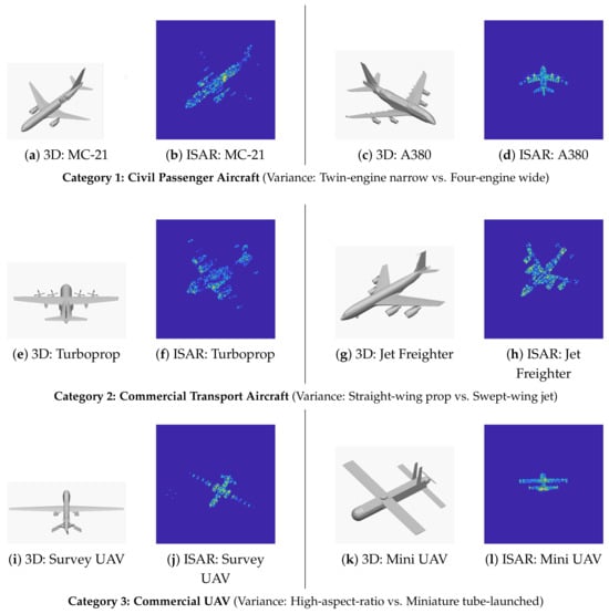
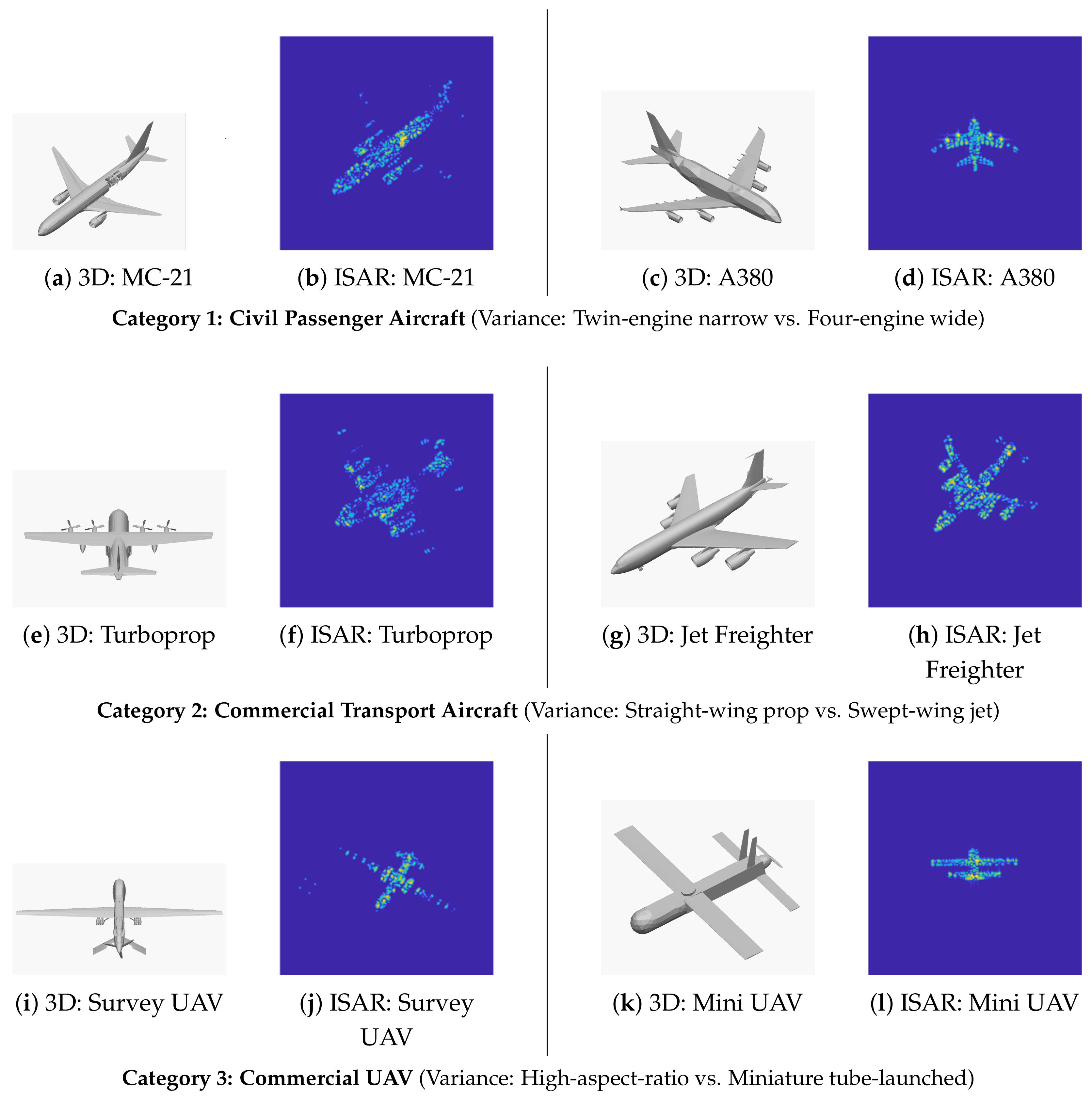
To evaluate true few-shot generalization and prevent the network from merely memorizing specific target contours, the dataset is hierarchically organized by functional categories rather than specific models. For instance, the “Civil Passenger Aircraft” category encompasses structurally diverse models such as the Airbus A380 (a four-engine, double-deck aircraft) and the MC-21 (a twin-engine, narrow-body aircraft). This multi-model aggregation increases intra-class variability, encouraging the network to learn high-level, generalized topological features of the category rather than overfitting to a single model’s isolated scattering points.
Representative 3D continuous surface models of 18 functional categories were acquired and converted into discrete point clouds using surface sampling algorithms to represent independent scattering centers. Radar echoes were simulated assuming an X-band high-resolution stepped-frequency radar. The detailed physical simulation parameters are listed in Table 1.
Table 1.
Core physical parameters for the ISAR echo simulation system.
Noise Configuration and Sample Distribution: To address real-world environmental interference, rigorous noise configurations were integrated. During the simulation phase, additive complex Gaussian white noise was injected into the baseband echo signals to maintain a constant Signal-to-Noise Ratio (SNR) of 20 dB. Furthermore, intrinsic multiplicative speckle noise, characteristic of coherent radar imaging systems, is naturally generated and preserved in the complex image domain.
Regarding sample distribution, the dataset was designed to capture comprehensive multi-angle representations. Each 3D target was rotated full-circle in azimuth from to with a precise step size of . This uniform spatial sampling yields exactly 240 ISAR images per model. During the meta-learning episode generation, query and support sets are sampled from these available views, ensuring a diverse and representative data distribution for each task without artificially constraining the global class sizes.
To eliminate Sinc-function sidelobe artifacts and retain sharp scattering points, the Spatially Variant Apodization (SVA) algorithm was employed during image reconstruction. Figure 1 intuitively illustrates the pipeline from 3D models to ISAR images, explicitly demonstrating how different models are grouped under unified categories. All resulting images were normalized and resized to pixels. The 18 categories were partitioned into 12 for meta-training, 3 for meta-validation, and 3 for meta-testing, ensuring zero category overlap between sets.
Figure 1.
The simulation pipeline mapping 3D CAD models to ISAR images. Structurally distinct models are grouped into broader functional categories to encourage the learning of generalized topological features.
2.2. Overview of Model Structure
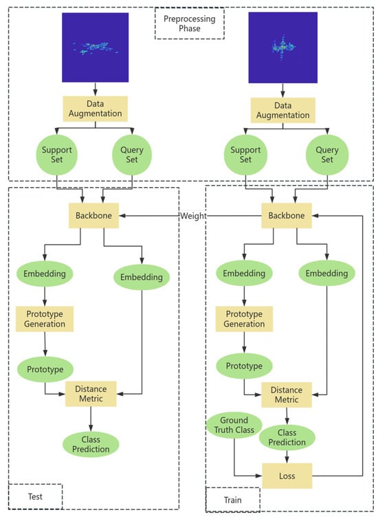
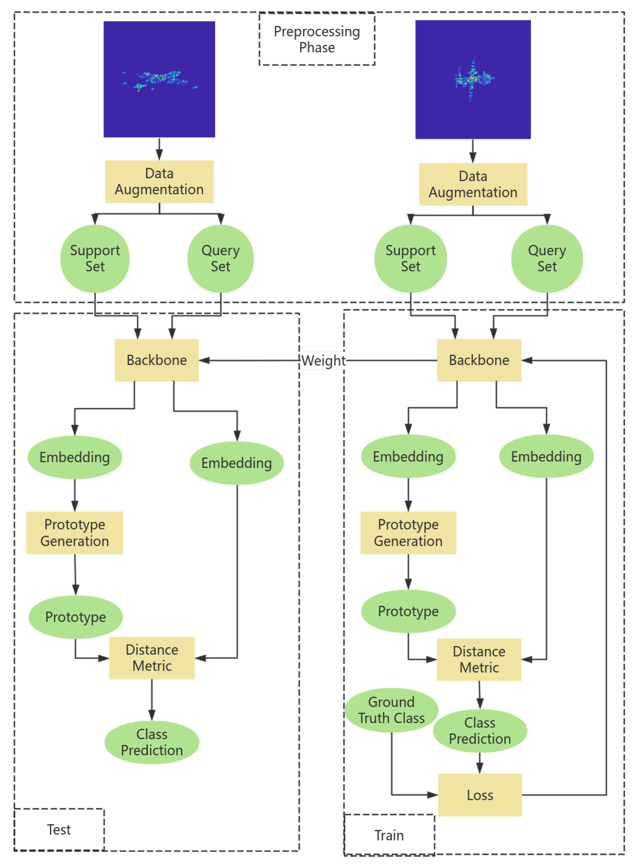
The proposed ISAR image classification framework based on Prototypical networks comprises three main components: a feature extraction layer, a prototype generation layer, and a distance-based classification layer. These components work collaboratively to achieve accurate and robust few-shot classification of ISAR images (Figure 2).
Figure 2.
Architecture of the prototypical network used in experiments. Colors are used for visual distinction only.
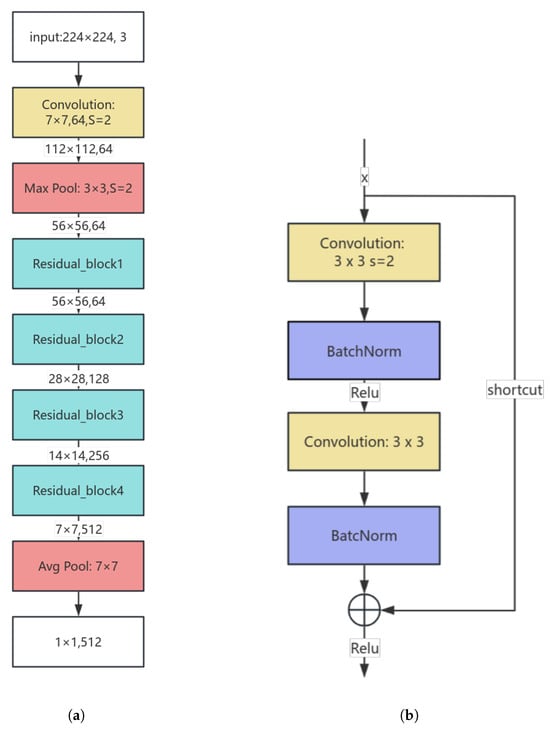
The feature extraction layer employs the ResNet10 architecture as the backbone. Owing to its residual connections, ResNet10 effectively mitigates gradient vanishing in shallow networks and enhances feature representation quality. When processing ISAR images, the network progressively extracts multiscale features such as scattering points, structural contours, and texture patterns through convolutional and pooling operations. This hierarchical extraction enables the model to capture both local scattering characteristics and global geometric structures critical to ISAR target recognition.
The prototype generation layer computes representative prototype vectors for each class using the mean feature embeddings of all samples in its support set. This aggregation captures the shared structural and scattering characteristics of each category while suppressing individual variations caused by aspect angle or attitude differences. Consequently, each prototype vector serves as a compact and discriminative representation of the target class.
The classification layer assigns query samples to the class whose prototype is closest in Euclidean space. Specifically, the Euclidean distance between the embedding of a query image and each class prototype is computed, and the class with the minimum distance is selected as the predicted label. This metric-based classification strategy allows efficient generalization to unseen categories under few-shot conditions.
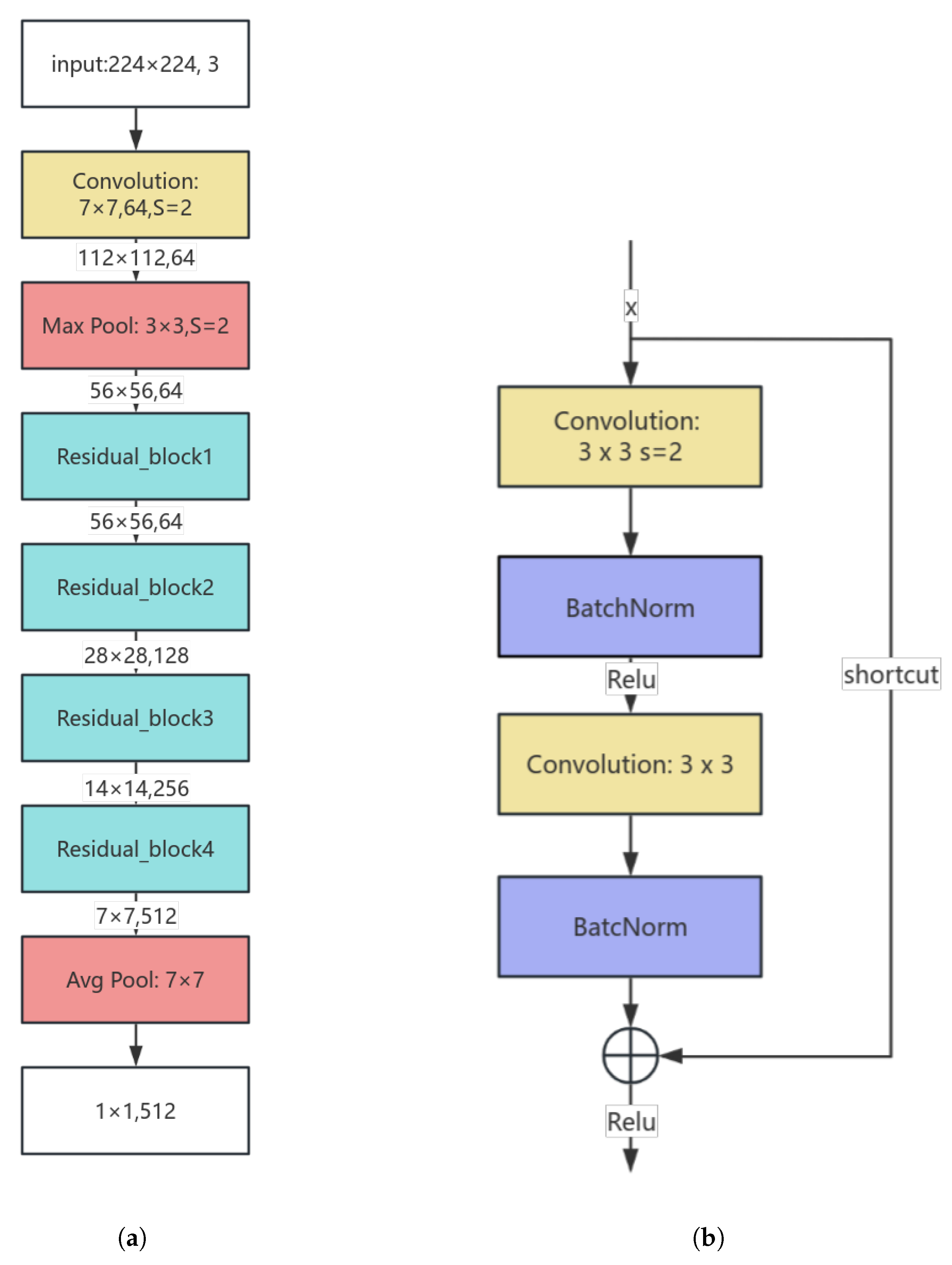
The ResNet10 backbone and the residual block used for feature extraction are shown in Figure 3.
Figure 3.
(a) Architecture of the ResNet10 feature extraction network. (b) Residual block structure. Colors are used for visual distinction only.
During model training, a joint loss function combining cross-entropy loss and the proposed AdaLoss is employed. The cross-entropy term ensures correct classification of query samples, while AdaLoss dynamically adjusts the inter-class margin based on prototype distances, thereby enhancing class separability. Through this integrated optimization, the network achieves superior OA and improved robustness in few-shot ISAR classification tasks.
2.3. AdaLoss: Noise-Tolerant Adaptive Relaxation Loss
In few-shot ISAR image classification, the fundamental criterion is to minimize the distance between a query sample and its class prototype. To establish a comparative baseline, we mathematically formulated a standard Hard Mining loss based on the classic Triplet Loss framework. For each query sample, it isolates the distance to its true class prototype () and actively mines the distance to the nearest, most confusing incorrect prototype (). The model is then strictly penalized using a clamping operation: . This operation forces the network to relentlessly separate all samples by a rigid, fixed margin , penalizing any sample that falls within this boundary. This hard constraint is completely agnostic to whether the sample’s difficulty stems from semantic similarity or severe noise corruption.
However, ISAR imagery poses a unique challenge: “hard” samples are often characterized by high speckle noise, distinct observation angles, or low resolution rather than semantic ambiguity. Enforcing strict large margins on these samples compels the network to overfit to high-frequency noise patterns, leading to optimization instability and reduced generalization.
To address this, we propose AdaLoss, which implements a Density-Based Adaptive Relaxation strategy. The core design philosophy is counter-intuitive but domain-specific:
- For easy samples (large inter-class distances), we apply standard constraints to ensure basic discriminability.
- For hard samples (small inter-class distances), we relax the margin constraints (assigning a smaller margin). This allows the model to tolerate a certain degree of feature overlap, preventing the gradient from being dominated by noisy outliers and preserving the global manifold structure.
The proposed total objective combines this Adaptive Relaxation term with the Cross-Entropy Loss (CeLoss), formulated as , where AdaLoss dynamically adjusts the margin value according to the prototype distance distribution. This adaptive mechanism enables the network to better capture the intrinsic inter-class separability of ISAR targets while maintaining the optimization stability provided by CeLoss.
The computation of AdaLoss involves four major steps: constructing distance matrices, determining the adaptive margin, calculating distances for positive and negative samples, and finally deriving the adaptive loss term to guide model optimization. The detailed process is as follows:
- (1)
- Construct Two Types of Basic Distance MatricesFirst, the query sample–class prototype distance matrix is defined. Let the query sample feature matrix be (where Q is the number of query samples and D is the feature dimension), and the class prototype matrix be (where C is the number of categories in the current episode). The elements of the distance matrix are defined as the Euclidean distances between each query feature vector and each class prototype vector.Second, the class prototype–class prototype distance matrix is constructed. This process begins with the construction of the original distance matrix between class prototypes, denoted as , and then adds a penalty term via a diagonal matrix to suppress the self-distance (distance from a prototype to itself, which is zero), resulting in the corrected matrix .
- (2)
- Generate the Adaptive MarginFirst, compute the minimum distance between class prototypes. For the corrected matrix , take the row-wise minimum to obtain the distance from each category c to the most similar prototype of another category:Subsequently, calculate the adaptive margin for each query sample q with upper and lower clipping bounds to prevent gradient explosion on exceptionally easy samples:where is the base margin value (, empirically validated via sensitivity analysis), and are the preset bounds. is the minimum inter-prototype distance corresponding to the true category of the query sample q, and is the mean of the minimum prototype distances across all categories, calculated as:
- (3)
- Filter Distances for Positive and Negative SamplesFirst, compute the positive sample distances. Let the true category label vector of the query samples be . For each query sample q, the positive sample distance is defined as the Euclidean distance between the query feature and the prototype of its true category :Next, compute the minimum negative sample distances. Let denote the previously computed distance matrix between query samples and all class prototypes, where each element represents the Euclidean distance between the q-th query sample and the c-th class prototype. Construct a mask matrix , where the position corresponding to the true category is set to 0 (excluded) and all other positions are set to 1 (retained). To avoid interference from the true-category distance when computing the minimum negative distance, a large penalty term of is added to these excluded positions. The corrected negative sample distance matrix is expressed as:Subsequently, the minimum negative sample distance (i.e., the distance to the most difficult-to-distinguish incorrect prototype) for each query sample q is obtained by taking the row-wise minimum:
- (4)
- Calculate the Final Margin LossThe optimization objective aims to ensure that the positive sample distance plus the adaptive margin is smaller than the negative sample distance. Formally, the constraint is defined as:If this condition is violated, a margin loss is computed to penalize the insufficient separation between positive and negative pairs. Otherwise, the loss is set to zero. The margin loss for each query sample is formulated as:Finally, the average margin loss over all query samples is computed to obtain the adaptive loss term:The final total loss combines the adaptive margin loss with the cross-entropy loss as follows:where denotes the cross-entropy loss.
3. Experimental Setup
3.1. Experimental Methods
The experiments were conducted under the standard C-way K-shot few-shot learning setting, where C denotes the number of classes and K represents the number of samples per class in the support set. To simulate the meta-task of few-shot ISAR image classification, a 3-way 5-shot configuration was adopted. In each meta-task, three categories were randomly selected, and five samples per category were used to form the support set.
During training, 10,000 meta-tasks were randomly sampled from the training subset. A cross-task meta-learning strategy was applied for optimization, with every 100 meta-tasks constituting one epoch. The model was trained for a total of 100 epochs, and the weights achieving the best performance on the validation set were retained for final testing. Each meta-task consisted of both a support set and a query set, with 10 query samples per class included for evaluation. In the testing phase, 100 meta-tasks were randomly sampled from the test subset, and the mean classification accuracy over all query sets was recorded as one evaluation.
To reduce random bias and enhance statistical reliability, this process was repeated 10 times, resulting in a total of 1000 meta-task evaluations. The final reported results are presented as the mean ± 95% confidence interval (CI) across repeated experiments, where the CI is computed as:
Here, represents the standard deviation and n denotes the number of repeated experiments.
For comparative analysis, several baseline few-shot models, including ProtoNet, RelationNet, and GauProto, were implemented under the same few-shot configuration. In addition, multiple backbone networks were evaluated to verify the effectiveness of the proposed architecture and the combined adaptive loss (CeLoss + AdaLoss).
All experiments were implemented using the PyTorch 2.0.1 framework (Python 3.10.11) with CUDA 11.7 and cuDNN 8.5.0 for GPU acceleration, on a workstation equipped with an NVIDIA GeForce RTX 4090 graphics card (NVIDIA, Santa Clara, CA, USA).
3.2. Performance Evaluation Metrics
A three-level evaluation framework is established to comprehensively assess the model performance.
3.2.1. Confusion Matrix
The confusion matrix is utilized to quantify the correspondence between predicted and actual categories, thereby reflecting the overall classification performance of the model [45]. The proportion of diagonal elements directly indicates the overall accuracy (OA), while the off-diagonal elements represent misclassified samples. For the 3-way ISAR classification task, the confusion matrix is represented as a square matrix and defined as follows:
- Horizontal axis (Predicted Category): Represents the predicted classes, denoted as , , and .
- Vertical axis (True Category): Represents the ground-truth categories, arranged in the same order as the predicted categories.
- Matrix elements: Let denote the number of samples whose true label belongs to class i but is predicted as class j. The diagonal elements indicate correctly classified samples, whereas the off-diagonal elements () correspond to misclassifications.
3.2.2. ROC Curve and AUC Value
The one-vs-rest (OvR) strategy is employed to decompose the multi-class classification task into multiple binary classification problems. The receiver operating characteristic (ROC) curve [46] is plotted with the false positive rate (FPR) on the x-axis and the true positive rate (TPR) on the y-axis. These fundamental metrics (TPR, FPR, TP, FN, etc.) are widely utilized to evaluate detection and classification performance across various remote sensing applications, such as SAR image change detection [47,48,49], heterogeneous image analysis [50,51], and infrared small ship detection [52,53]. They are defined respectively as:
where and denote the numbers of false positives and true negatives, respectively, while and represent the numbers of true positives and false negatives. The area under the curve (AUC) is then calculated to quantitatively evaluate the classifier’s overall separability. A higher AUC value indicates stronger discriminative capability and greater reliability in distinguishing between different target categories.
3.2.3. Core Classification Metric
The overall accuracy (OA) [44] is adopted as the primary evaluation metric and is calculated as:
A higher OA value indicates better classification performance across few-shot ISAR recognition tasks.
4. Results
4.1. Comparative Experiments with State-of-the-Art Baselines
To validate the effectiveness of the proposed model, we organized the comparative experiments into a progressive evaluation framework. First, we assessed classical few-shot metric models (ProtoNet [43], RelationNet [54], and GauProto [55]) across various backbone architectures to determine the optimal feature extractor for ISAR imagery. Second, we compared our AdaProtoNet against recent State-of-the-Art (SOTA) algorithms.
As shown in Table 2, GauProto underperforms on ISAR data because its multivariate Gaussian assumption cannot capture the highly fragmented scattering manifolds caused by aspect-angle scintillation. ProtoNet utilizing the lightweight ResNet10 backbone achieves the highest baseline accuracy (70.71%), suggesting that Euclidean metric learning coupled with residual connections provides a stable foundation for noisy radar features.
Table 2.
Comparison of overall accuracy (OA (%) ± 95% CI) across classical baseline models under 3-way 5-shot condition.
To rigorously benchmark our method against recent advancements, we compared AdaProtoNet with highly competitive SOTA frameworks, including FEAT [56], MetaOptNet [57], and SSLProtoNet [58]. To ensure absolute fairness and avoid redundant evaluations on sub-optimal shallow networks, all SOTA methods were evaluated specifically on the primary optimal backbone (ResNet10).
The results in Table 3 reveal crucial insights. Advanced methods like MetaOptNet perform reasonably well (69.10%), and SSLProtoNet achieves a competitive 72.58% by leveraging self-supervised representations to mitigate noise. However, our AdaProtoNet achieves the highest OA of 77.45%. This demonstrates that generic computer vision (CV) few-shot methods—which rely on complex meta-optimization or self-supervision—still struggle with ISAR speckle noise. In contrast, our domain-specific “Adaptive Relaxation” mechanism directly addresses radar feature ambiguity.
Table 3.
Comparison with SOTA few-shot learning methods on the optimal backbone (ResNet10).
Interestingly, the FEAT model experienced a performance decrease on ResNet10 (51.32%). To investigate this phenomenon and highlight the efficiency considerations of certain SOTA methods in radar applications, we conducted a detailed computational complexity analysis of FEAT across all backbones (Table 4).
Table 4.
Computational complexity and performance collapse of FEAT with different backbones.
FEAT employs an advanced Set-to-Set attention mechanism to adapt embeddings. However, as shown in Table 4, this introduces a higher computational requirement when coupled with residual networks. For instance, FEAT with a ResNet10 backbone requires 157.86 G FLOPs, while its accuracy drops to 51.32%, likely due to the attention module overfitting to the sparse ISAR scattering centers.
In comparison, our AdaProtoNet relies on Euclidean distance, requiring 0.89 G FLOPs with the exact same ResNet10 backbone (as detailed in the ablation studies). This demonstrates that AdaProtoNet achieves higher accuracy (77.45% vs. 51.32%) with less computational cost compared to FEAT, establishing it as an efficient framework for resource-constrained real-time radar systems.
4.2. Feature Space Representation and Spatial Analysis
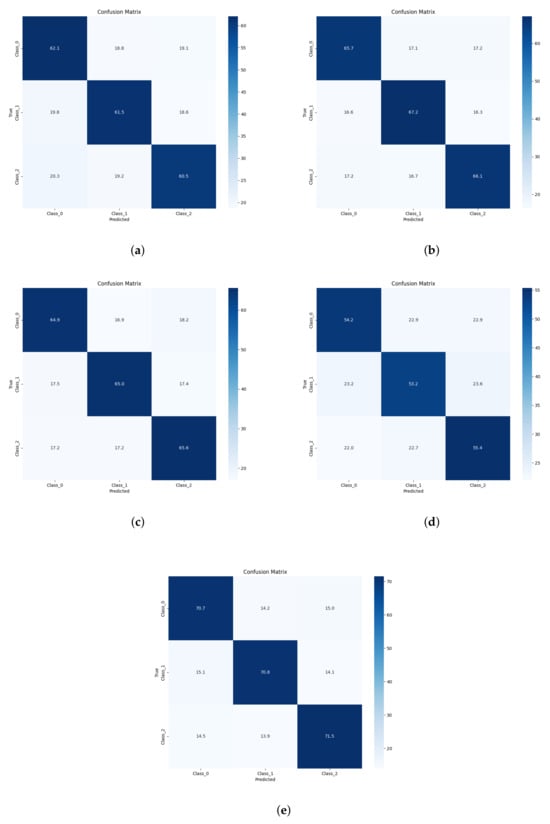
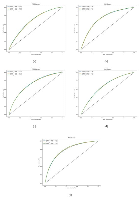
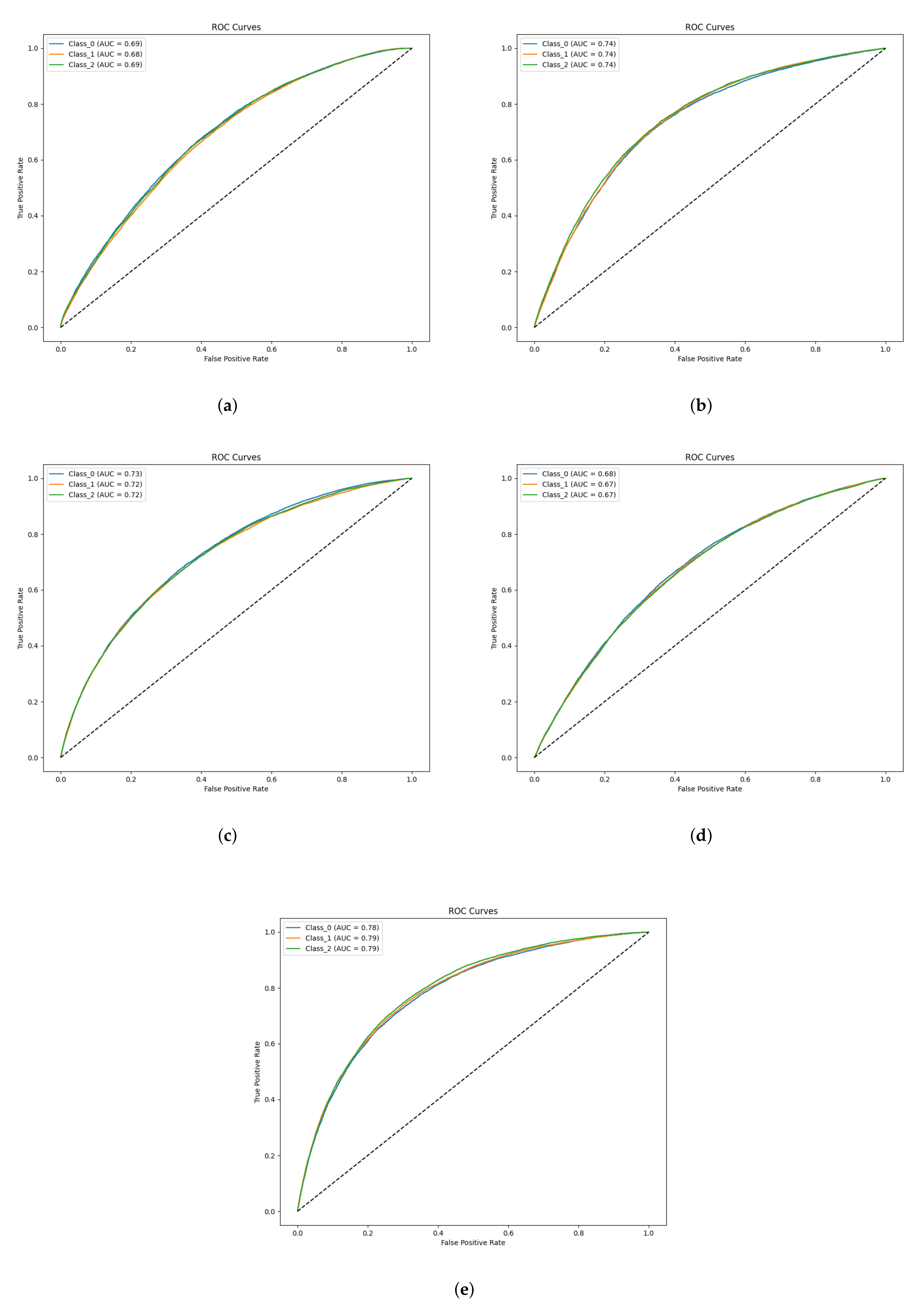
To provide an intuitive spatial interpretation of how ProtoNet shapes the feature metric space under different backbones, we analyze the Confusion Matrices [45] (Figure 4) and the corresponding ROC curves [46] (Figure 5) for a typical 3-way 5-shot test task.
Figure 4.
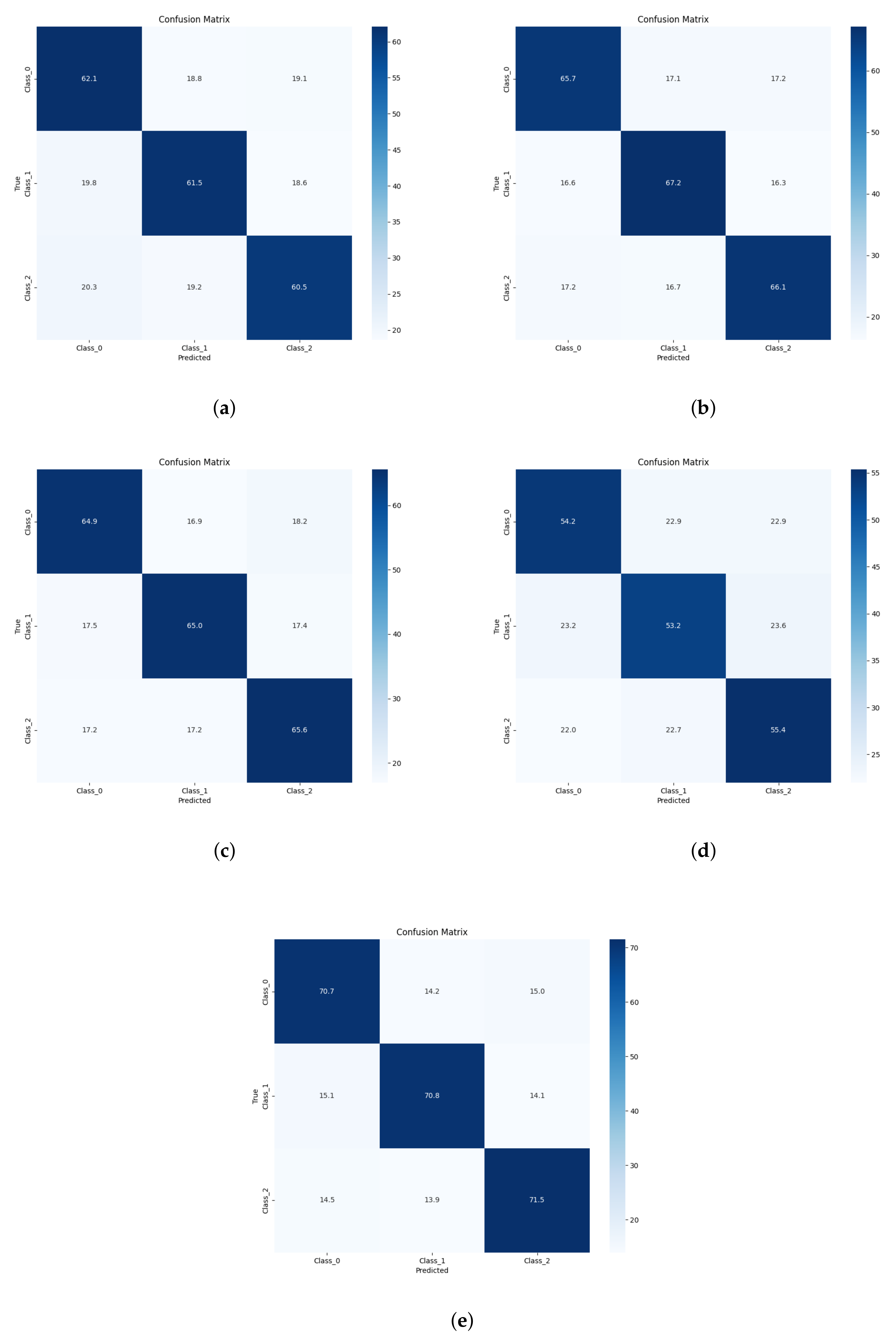
Comparison of Confusion Matrices: prototype network with ResNet10 backbone vs. other backbones ((a–e): Conv4, Conv6, ResNet18, ResNet34, ResNet10 backbones respectively).
Figure 5.
ROC curve comparison of different backbones ((a–e): Conv4, Conv6, ResNet18, ResNet34, ResNet10 backbone). The dashed diagonal line represents the performance of a random guess classifier.
Observing Figure 4d, when using a deeper ResNet34 backbone [59], the off-diagonal areas of the confusion matrix show increased values. This indicates inter-class penetration at the boundaries. The network may use its representational capacity to fit idiosyncratic high-frequency edge artifacts unique to specific samples. Consequently, any slight shift in these artifact patterns causes the query sample to be misclassified.
Conversely, ResNet10 (Figure 4e) suppresses off-diagonal elements, achieving correctly predicted proportions of 70.7%, 70.8%, and 71.5% across classes, demonstrating a balanced distribution. This confirms that our chosen feature mapping layer maintains consistency and inter-class mutual exclusivity when processing heterogeneous ISAR categories.
The ROC curves in Figure 5 provide further observation. While the curves for the Conv-series networks tend towards the random guess axis due to insufficient receptive fields, the ResNet10 ROC curve (Figure 5e) presents a clear rising edge. Its AUC integral values consistently exceed 0.78 across all categories. This confirms the model’s capacity to identify the true identity of query targets under a low false-positive rate in the 5-shot scenario.
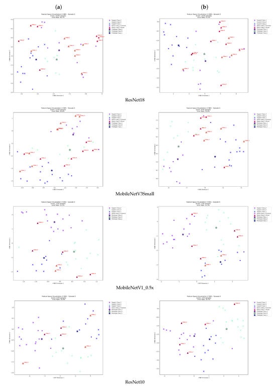
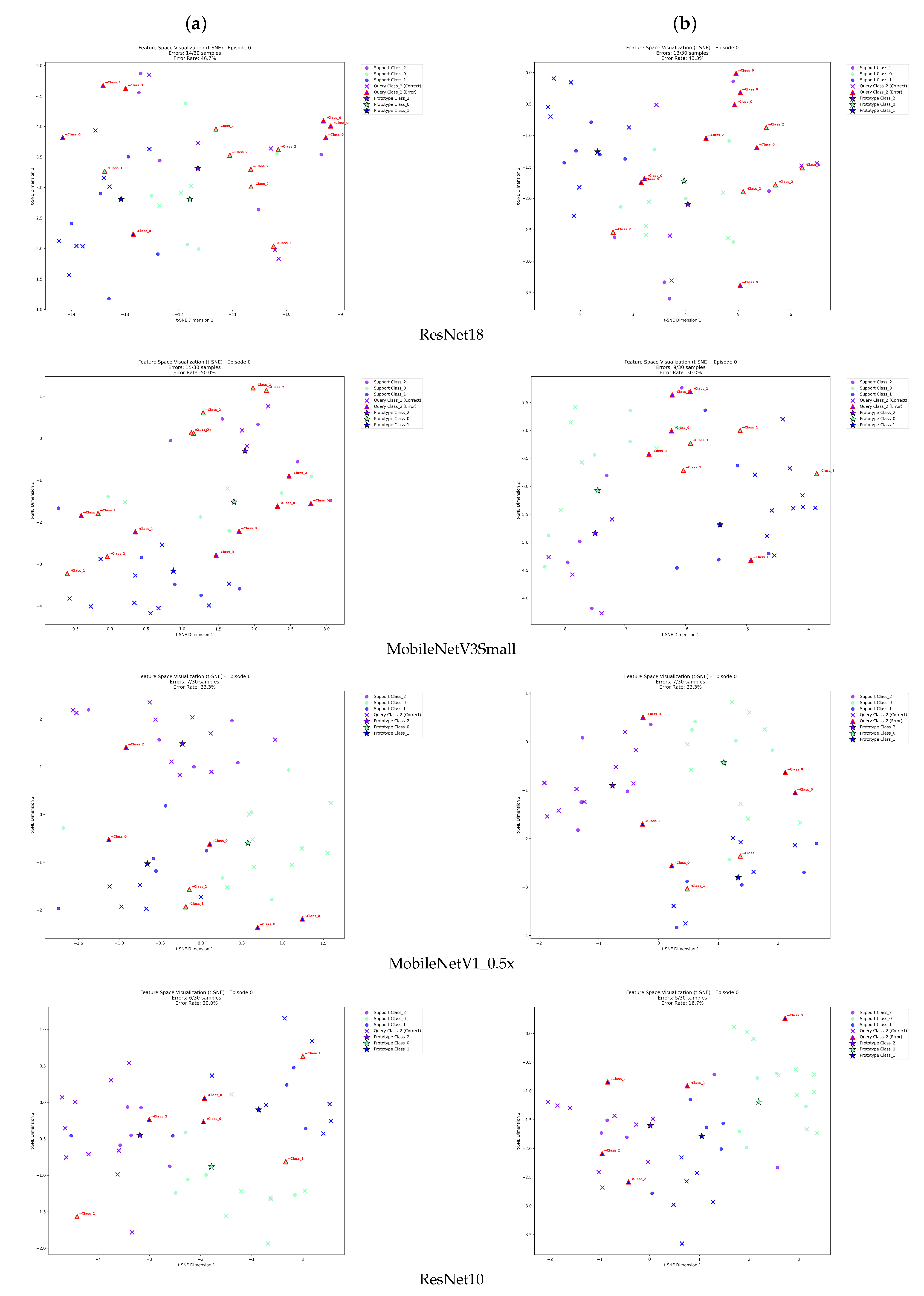
To further provide visual evidence regarding intra-class compactness and inter-class separability at the manifold level, we utilized the t-SNE algorithm [60] to map the identical batch of feature embeddings into a 2D space across different backbone and loss combinations (Figure 6).
Figure 6.
Scatter plots of feature distributions for the same batch of samples. The left column (a) corresponds to CeLoss; the right column (b) corresponds to CeLoss + AdaLoss. In the scatter plots, solid circles (●) represent support samples, stars (★) denote class prototypes, and crosses (×) indicate correctly classified query samples, where the color matches the true class. Misclassified query samples are highlighted with red triangle borders (△) and annotated with red text indicating their mispredicted class labels.
Focusing on the final row (ResNet10), Figure 6a shows that while CeLoss forms preliminary clusters, several isolated, difficult samples drift loosely near the decision boundaries, indicating weak constraint on ambiguous points. In Figure 6b, aided by the Adaptive Relaxation mechanism, the network gracefully handles these hard, noise-corrupted points. Rather than forcing them apart—which would shatter the manifold—the relaxed margins allow them to be safely encompassed within their respective clusters, significantly tightening intra-class variance and clearing the inter-class void.
4.3. Ablation and Parameter Sensitivity Analysis
Ablation experiments were conducted to evaluate the impact of various backbone networks (including lightweight networks like ShuffleNet and EfficientNet) and to quantify computational efficiency.
Table 5 reveals that extremely shallow networks (ResNet6) lack representation capacity, while deeper networks (ResNet18) overfit. Classical architectures such as AlexNet [61] and GoogLeNet [62] were also evaluated in preliminary tests but failed to achieve competitive performance due to their parameter-heavy or complex inception designs, which struggle to generalize on sparse ISAR data. Interestingly, lightweight architectures using Depthwise Separable Convolutions (ShuffleNet, EfficientNet) perform worse than ResNet10. This is because ISAR scattering centers are discrete bright spots whose topological relationships rely heavily on cross-channel correlations, which standard dense convolutions (ResNet10) preserve better than depthwise convolutions.
Table 5.
Ablation of backbone networks: accuracy, parameter size, and inference efficiency.
To quantitatively evaluate the additional computational cost introduced by AdaLoss, we measured the average training time per episode (including the forward pass, loss computation, and backpropagation) on an RTX 4090 GPU under the 3-way 5-shot setting. Empirical measurements indicate that training the ResNet10 backbone with standard CeLoss [67] takes approximately 15.708 ms per episode, whereas training with the proposed CeLoss + AdaLoss takes 16.158 ms. This demonstrates that computing the adaptive margins and distance matrices introduces a negligible training overhead of only 0.450 ms (a relative increase of approximately 2.86%). Furthermore, because AdaLoss operates exclusively on low-dimensional embedding vectors during the training phase, it introduces zero additional computational overhead during the inference and deployment phase.
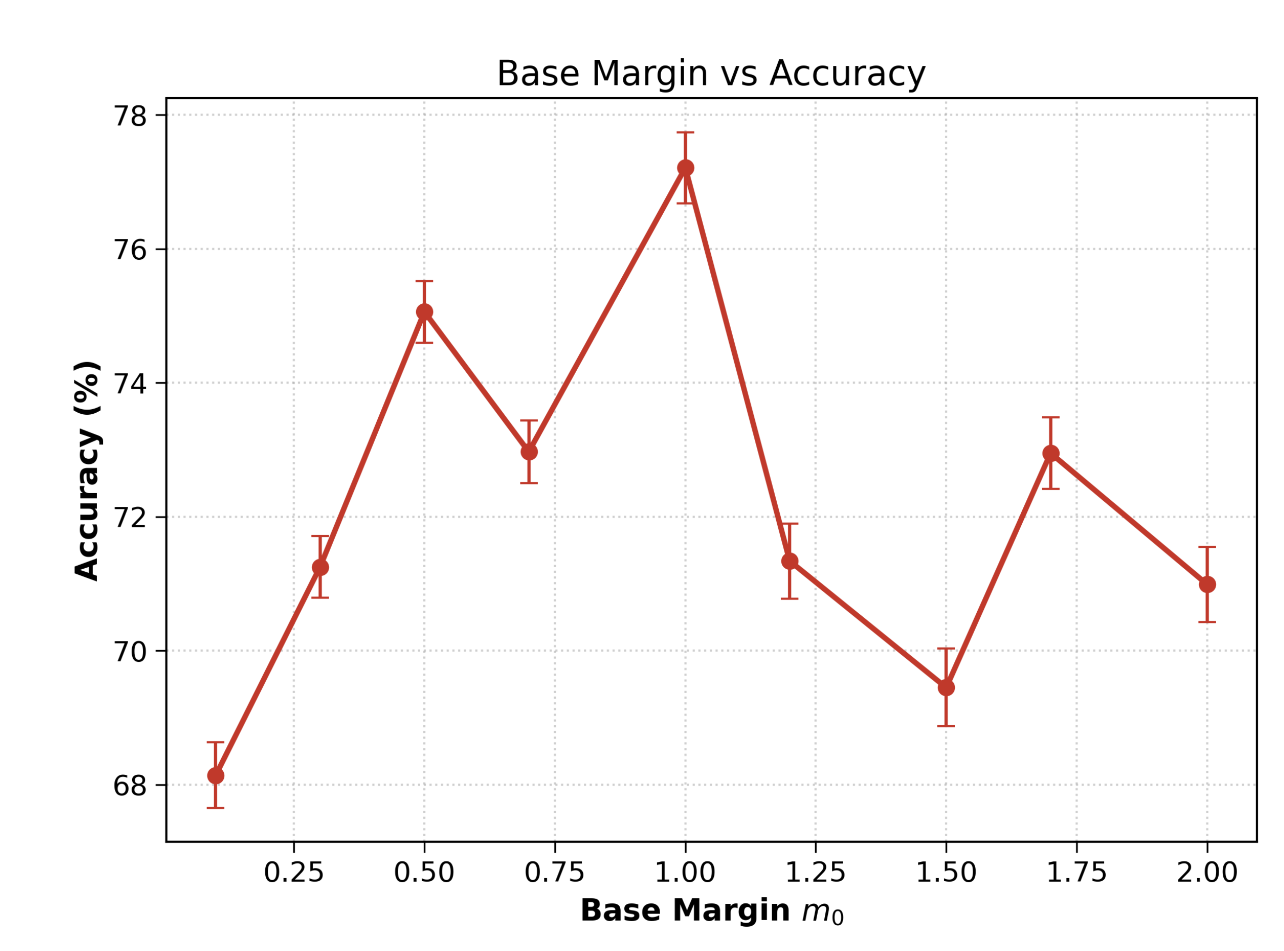
To rigorously justify the empirical setting of the base margin in Equation (2) and to address the sensitivity of the model to this hyperparameter, we conducted a comprehensive sensitivity analysis. We evaluated the overall accuracy of AdaProtoNet (with ResNet10 backbone) across a wide range of values from 0.1 to 2.0 under the 3-way 5-shot setting.
As illustrated in Figure 7, the model performance exhibits a clear inverted-U trajectory, confirming that is the optimal “sweet spot.”
Figure 7.
Sensitivity analysis of the base margin m0. The curve displays the Overall Accuracy (%) and its 95% confidence interval across different m0 settings. The peak performance is unequivocally achieved at m0 = 1.0.
The underlying mechanism driving this trend perfectly aligns with our physics-informed relaxation philosophy:
- (1)
- Under-constrained Regime (): When the base margin is too small, the resultant adaptive margin lacks sufficient repulsive force to separate inter-class prototypes in the Euclidean space. The metric constraint becomes overly loose, causing the model to lose its discriminative power and degrade toward the baseline CeLoss performance (around 68% at ).
- (2)
- Optimal Balance Regime (): At exactly 1.0, the base margin perfectly balances the adaptive ratio . It provides robust separation for easy ISAR targets while allocating a mathematically precise “tolerance buffer” for ambiguous, noise-corrupted samples, reaching a peak accuracy of 77.45%.
- (3)
- Over-constrained Regime (): As becomes aggressively large, the absolute margin enforced on noisy samples becomes exceedingly high, even after the Adaptive Relaxation ratio is applied. This completely overrides the “relaxation” philosophy, forcing the network back into the “Hard Mining” trap. Consequently, the network overfits to high-frequency speckle artifacts, leading to a precipitous drop and severe instability in classification accuracy (dropping below 70% at ).
Therefore, maintaining a fixed provides the optimal trade-off between category discriminability and noise tolerance, avoiding the additional computational overhead of making it a learnable parameter during the few-shot meta-training phase.
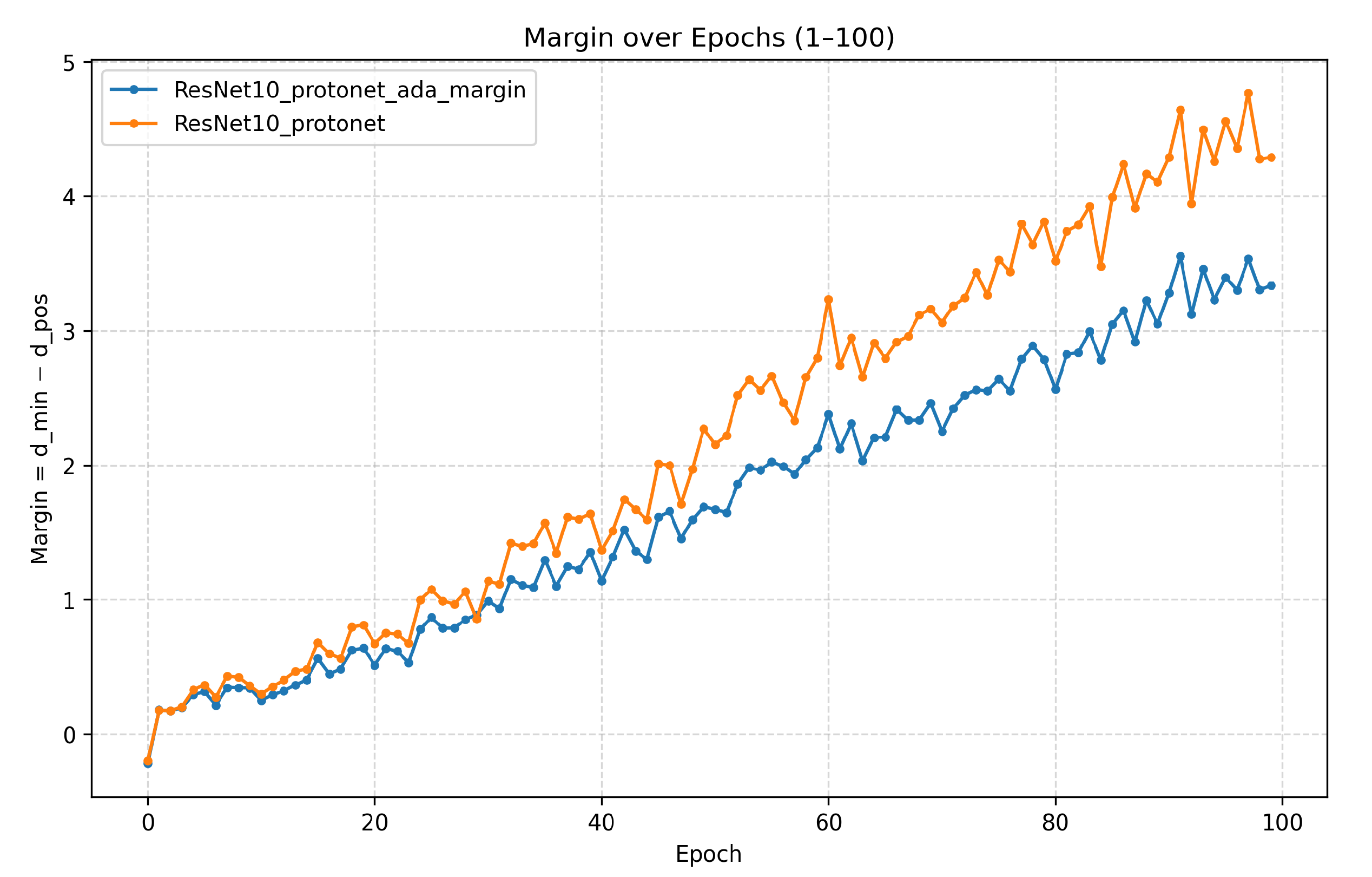
To further verify the training stability provided by the Adaptive Relaxation strategy, we visualized the evolution of the classification margin during the training process. As shown in Figure 8, we tracked the margin value over 100 epochs for both the baseline ResNet10-ProtoNet and our AdaProtoNet.
Figure 8.
Comparison of training margin evolution over 100 epochs. The blue curve represents ResNet10 with AdaLoss (Ours), while the orange curve represents the baseline ResNet10 with standard loss. The baseline model forces an aggressively large margin, indicating overfitting to speckle noise, whereas AdaProtoNet maintains a smooth and stable margin, preventing over-optimization on hard samples.
In the context of metric learning, this margin is defined as , where is the distance between a query sample and its true class prototype, and is the distance to the nearest (most confusing) incorrect class prototype. A positive and growing margin indicates that the model is successfully pulling samples closer to their correct class centers while pushing them away from decision boundaries. Conversely, severe fluctuations or negative values imply that the model is struggling with hard samples, causing decision boundaries to collapse.
The comparison reveals a critical insight into the optimization behavior. The baseline model (orange) exhibits a steep, monotonic increase, aggressively forcing the margin larger and larger. While this might appear beneficial in standard clean datasets, in the context of ISAR imagery, it indicates that the network is desperately overfitting to high-frequency speckle artifacts in an attempt to forcefully pull apart inherently ambiguous, noise-corrupted samples.
In stark contrast, AdaProtoNet (blue) demonstrates a significantly smoother trajectory. Once the margin safely crosses the zero threshold (indicating correct classification), it does not aggressively pursue an excessively large distance. By dynamically relaxing the constraints on these hard, noisy samples, AdaLoss ensures the margin grows steadily and remains bounded. This smoother evolution proves that the network successfully avoids overfitting to noise, focusing instead on learning generalized, robust topological features.
4.4. Robustness and Real-World Validation (MSTAR)
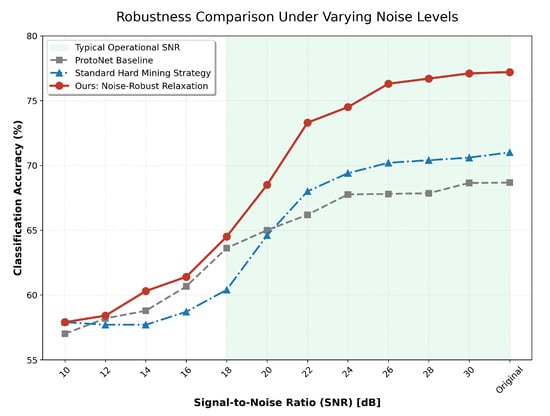
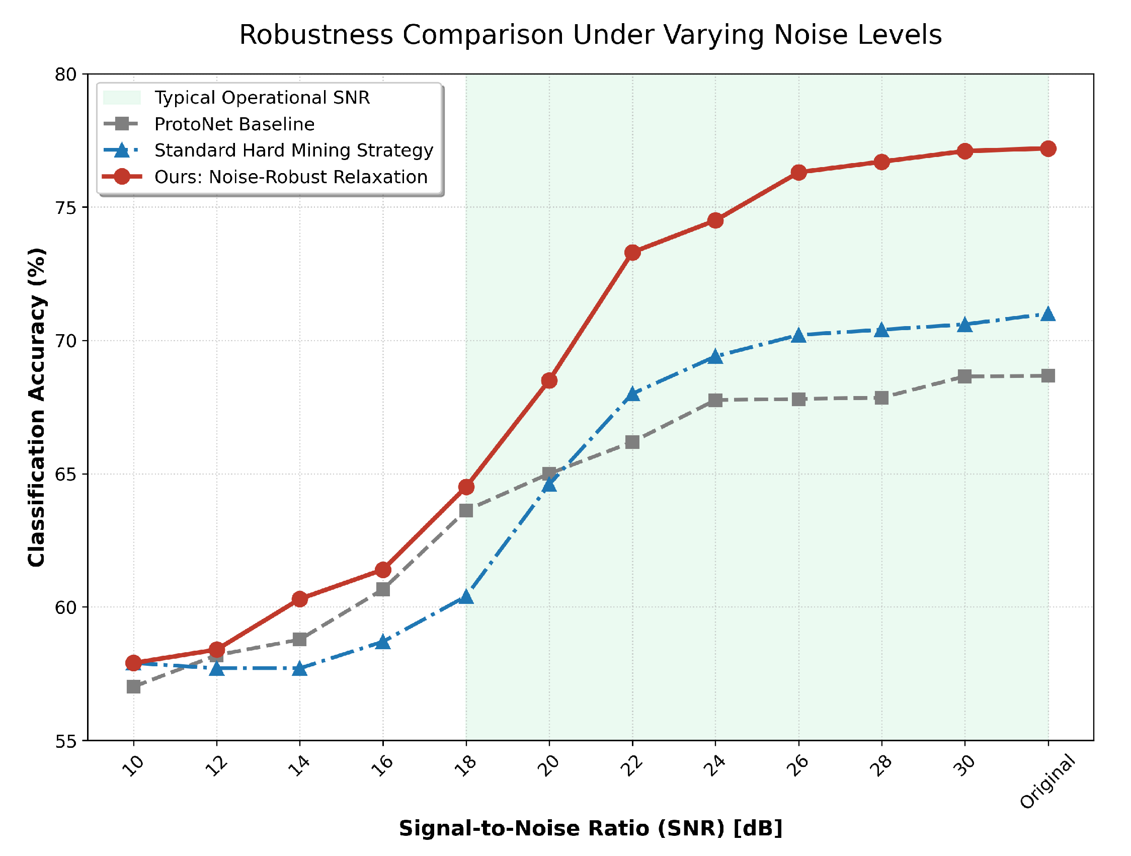
We first conducted a robustness analysis by replacing standard Gaussian noise with realistic radar Multiplicative Speckle Noise. The noise model follows a Gamma distribution, which is widely used to characterize the fully developed speckle in coherent radar imaging systems. The noisy image Y is generated from the clean image X as , where N represents the speckle noise following a Gamma distribution with mean 1 and variance , where L is the number of looks. By varying L, we simulate different Signal-to-Noise Ratio (SNR) levels to rigorously test the model’s resilience against signal-dependent interference.
As shown in Figure 9, this standard Hard Mining strategy based on Triplet Loss (blue curve) exhibits significant degradation under severe speckle noise, notably falling below the ProtoNet Baseline (grey curve) in the 12–20 dB range. Because speckle noise is signal-dependent (brighter scattering centers are noisier), blindly enforcing a rigid margin on these corrupted samples causes the network to severely distort high-intensity structural features. In contrast, our proposed Adaptive Relaxation (red curve) demonstrates superior robustness, maintaining an accuracy of approximately 64.5% at the 18 dB threshold, and rapidly recovering to 74.5% at 24 dB. Through distance evolution tracking and sensitivity analysis, the base margin was confirmed to stably provide this optimal tolerance buffer.
Figure 9.
Robustness comparison under varying Multiplicative Speckle Noise (SNR) levels.
To rigorously address the “sim-to-real” domain gap and validate the practical applicability of our framework beyond simulated noise, we conducted a highly challenging cross-domain zero-shot transfer experiment. The models were exclusively trained on our custom simulated ISAR dataset and subsequently tested directly on the publicly available real-world MSTAR SAR dataset [68] without any fine-tuning, under a 3-way 5-shot condition.
The cross-domain transfer results across various backbone architectures are presented in Table 6. Directly applying models trained on simulated data to real-world measured data typically results in severe performance degradation due to unmodeled background clutter and real speckle noise distributions. As observed, the baseline models trained with standard CeLoss suffer from poor cross-domain accuracy (e.g., EfficientNet-Lite0 at 47.24%, MobileNetV3Small at 49.07%). This confirms our hypothesis that traditional hard-margin learning forces the network to overfit to the simulation-specific high-frequency artifacts (such as synthetic background cleanliness), thereby ruining its generalization to real-world physical scattering.
Table 6.
Cross-domain sim-to-real transfer performance on the real-world MSTAR dataset (models were exclusively trained on simulated ISAR and tested directly on MSTAR under 3-way 5-shot condition).
In contrast, the models trained with the proposed AdaLoss (CeLoss + AdaLoss) demonstrate significantly enhanced transferability across almost all backbones. For instance, MobileNetV3Small achieves a substantial absolute improvement of 7.77% (from 49.07% to 56.84%), and EfficientNet-Lite0 improves by 4.06%. For our primary ResNet10 backbone, the AdaLoss mechanism evaluated at the optimal base margin () achieved a stable transfer accuracy of 53.27%.
These results provide compelling empirical evidence that the “Adaptive Relaxation” strategy acts as a powerful structural regularizer. By relaxing the strict margin requirements on noisy or artifact-heavy simulated samples during training, AdaLoss successfully prevents the network from memorizing the simulation domain biases. Instead, it guides the model to learn the fundamental, domain-invariant electromagnetic topological layouts of the targets, remarkably bridging the sim-to-real gap for radar recognition systems.
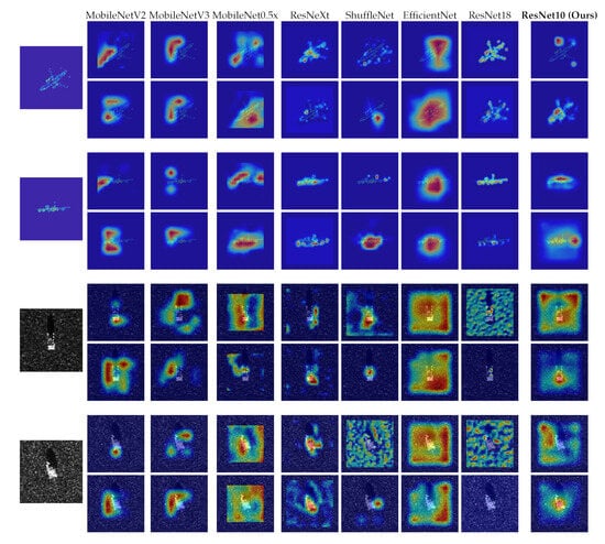
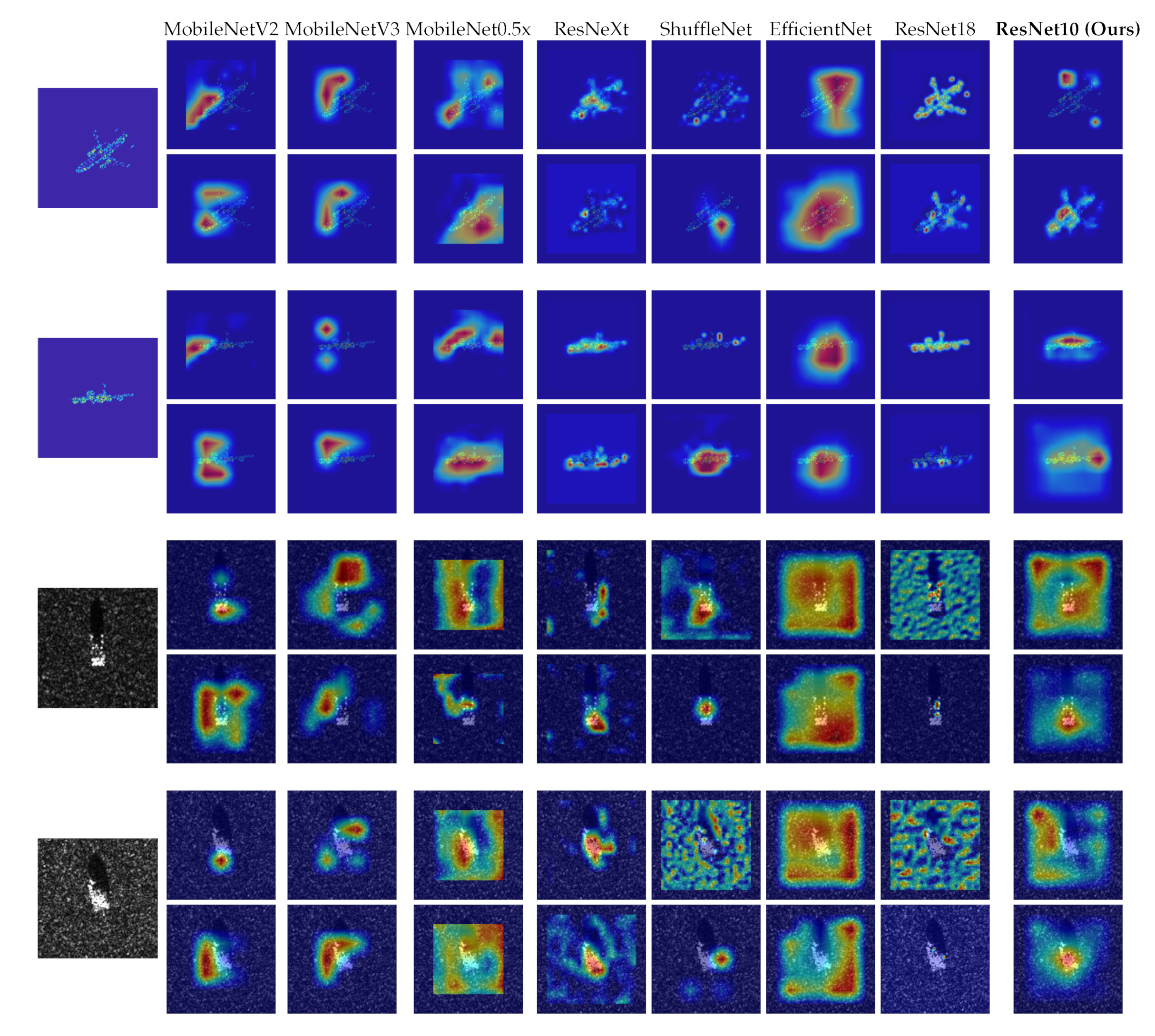
To bridge the gap between simulation and practice, and to demystify the internal decision-making process of AdaLoss, we conducted supplementary validation using the real-world MSTAR SAR dataset. We utilized Gradient-weighted Class Activation Mapping (Grad-CAM) [69] to visualize the attention heatmaps for both our custom simulated ISAR images and real MSTAR images across different models.
As visualized in Figure 10, models trained solely with standard CeLoss (and hard-mining strategies) exhibit scattered attention. Their activation regions drift into the noisy background clutter, indicating they may be learning speckle artifacts. In contrast, models optimized with the AdaLoss relaxation strategy exhibit concentrated, structurally logical attention maps. The network focuses on the true electromagnetic scattering centers of the targets (e.g., wing structures, vehicle edges), effectively ignoring background clutter. This experiment indicates that AdaProtoNet is physically interpretable and can generalize to real-world SAR measured data.
Figure 10.
Grad-CAMvisualization comparison. Each block corresponds to a target. The first column shows the original image. The subsequent columns showthe attentionmaps for 8models. For eachmodel column, the top image is the baseline (CeLoss) and the bottomimage is the proposed (CeLoss + AdaLoss). Red regions indicate high attention weights, while blue regions indicate low attention weights.
5. Discussion
The experimental results validate the efficacy of AdaProtoNet for few-shot ISAR image classification, offering several important insights into radar target recognition.
First, the superiority of the ResNet10 backbone in the Prototypical Network framework indicates a critical balance in model complexity. While extremely lightweight models suffer from insufficient representational capacity to capture complex cross-channel spatial scattering relations, overly deep networks tend to overfit to the severe speckle noise inherent in ISAR imagery. The residual connections in ResNet10 provide an optimal trade-off, enabling robust feature extraction without catastrophic overfitting.
Second, the introduction of the Adaptive Relaxation Strategy (AdaLoss) addresses a fundamental flaw in applying traditional metric learning to radar data. Conventional hard-mining techniques assume that difficult samples carry semantic structural similarities. However, in ISAR images, hard samples are overwhelmingly caused by severe noise corruption or extreme aspect-angle scintillation. By dynamically relaxing the margin for these noisy samples, AdaLoss prevents the shattering of the underlying topological manifold, as clearly demonstrated by our t-SNE visualizations. This mechanism ensures that the network learns generalized structural features rather than memorizing high-frequency noise artifacts.
Third, the Grad-CAM visualizations on both simulated ISAR data and the real MSTAR dataset confirm the physical interpretability of the proposed method. The attention maps prove that AdaProtoNet focuses strictly on genuine physical scattering centers rather than background clutter, ensuring that the classification is driven by reliable radar signatures.
Despite these advances, a limitation remains: classification performance still experiences noticeable degradation under extremely low Signal-to-Noise Ratio (SNR) conditions (e.g., <15 dB) where the target’s scattering topology is completely submerged in noise. Future work will explore the integration of Complex-Valued Neural Networks (CVNNs) to directly exploit the rich phase information preserved in raw radar echoes, and develop end-to-end joint denoising-recognition architectures tailored for extreme electromagnetic environments.
6. Conclusions
This paper proposed AdaProtoNet, a novel few-shot classification framework tailored for ISAR images. By jointly developing a custom multi-scenario ISAR dataset, a ResNet10-based Prototypical Network, and a physics-informed Adaptive Relaxation Strategy (AdaLoss), this study successfully addressed the challenges of data scarcity and severe speckle noise interference in radar target recognition.
The main findings confirm that: (1) The ResNet10 backbone provides optimal inter-class separability and avoids the gradient vanishing issues seen in shallower models; (2) AdaLoss significantly enhances noise robustness by dynamically adjusting optimization margins, achieving an overall accuracy of 77.45% on the custom dataset and outperforming traditional hard-mining approaches; and (3) visual interpretations via Grad-CAM verify the model’s strong real-world applicability and its ability to focus on authentic physical scattering centers. Ultimately, AdaProtoNet offers a highly robust and interpretable solution for few-shot remote sensing recognition, paving the way for more reliable maritime and aerospace surveillance systems.
Author Contributions
Conceptualization, Z.Z. and M.L.; methodology, Z.Z. and L.L.; software, Z.J.; validation, H.M. and X.Z. (Xueyu Zhang); formal analysis, Z.Z.; investigation, M.L.; resources, H.M.; data curation, X.Z. (Xiaobin Zhao); writing—original draft preparation, Z.Z.; writing—review and editing, L.L. and H.M.; visualization, Z.Z.; supervision, H.M.; project administration, L.L.; funding acquisition, Z.J. and H.M. All authors have read and agreed to the published version of the manuscript.
Funding
This research was funded by the National Natural Science Foundation of China under Grant Nos. 62261053 and 62401062; the Tianshan Talent Training Project–Xinjiang Science and Technology Innovation Team Program (2023TSYCTD0012); and the Research Project of Xinjiang Sky-Ground Integrated Intelligent Computing Technology Laboratory under Grant No. 2025A05-1.
Data Availability Statement
The data presented in this study are available on request from the corresponding author.
Acknowledgments
The authors acknowledge the support from the Key Laboratory of Signal Detection and Processing at Xinjiang University.
Conflicts of Interest
The authors declare no conflicts of interest.
References
- Vehmas, R.; Neuberger, N. Inverse Synthetic Aperture Radar Imaging: A Historical Perspective and State-of-the-Art Survey. IEEE Access 2021, 9, 113917–113943. [Google Scholar] [CrossRef] [Scilit]
- Bai, X.R.; Yang, M.J.; Chen, B.W.; Zhou, F. REMI: Few-Shot ISAR Target Classification via Robust Embedding and Manifold Inference. IEEE Trans. Neural Netw. Learn. Syst. 2025, 36, 6000–6013. [Google Scholar] [CrossRef] [Scilit] [PubMed]
- Deng, J.; Su, F.L. Deep Hybrid Fusion Network for Inverse Synthetic Aperture Radar Ship Target Recognition Using Multi-Domain High-Resolution Range Profile Data. Remote Sens. 2024, 16, 3701. [Google Scholar] [CrossRef] [Scilit]
- Xue, R.H.; Bai, X.R.; Zhou, F. SAISAR-Net: A Robust Sequential Adjustment ISAR Image Classification Network. IEEE Trans. Geosci. Remote Sens. 2021, 60, 5214715. [Google Scholar] [CrossRef] [Scilit]
- Yang, H.; Zhang, Y.S.; Yin, C.B.; Ding, W.Z. Ultra-lightweight CNN Design Based on Neural Architecture Search and Knowledge Distillation: A Novel Method to Build the Automatic Recognition Model of Space Target ISAR Images. Def. Technol. 2022, 18, 1073–1095. [Google Scholar] [CrossRef] [Scilit]
- Xue, B.; Tong, N.N.; Xu, X. DIOD: Fast, Semi-Supervised Deep ISAR Object Detection. IEEE Sens. J. 2019, 19, 1073–1081. [Google Scholar] [CrossRef] [Scilit]
- Rosenberg, L.; Zhao, W.; Heng, A.; Hamey, L.; Nguyen, S.T.; Orgun, M.A. Classification of ISAR Ship Imagery Using Transfer Learning. IEEE Trans. Aerosp. Electron. Syst. 2024, 60, 25–36. [Google Scholar] [CrossRef] [Scilit]
- Manno-Kovacs, A.; Giusti, E.; Berizzi, F.; Kovács, L. Image Based Robust Target Classification for Passive ISAR. IEEE Sens. J. 2019, 19, 268–276. [Google Scholar] [CrossRef] [Scilit]
- Liu, J.; Qin, C.H.; Zhan, Y.Y.; Wang, F.J.; Tu, J. ISAR Image Target Recognition Based on Convolutional Neural Network. Guid. Fuze 2024, 45, 27–34. [Google Scholar] [CrossRef]
- Rong, J.; Wang, Y.; Han, T. Iterative Optimization-Based ISAR Imaging with Sparse Aperture and Its Application in Interferometric ISAR Imaging. IEEE Sens. J. 2019, 19, 8681–8693. [Google Scholar] [CrossRef] [Scilit]
- Li, R.; Zhang, S.; Zhang, C.; Liu, Y.; Li, X. Deep Learning Approach for Sparse Aperture ISAR Imaging and Autofocusing Based on Complex-Valued ADMM-Net. IEEE Sens. J. 2021, 21, 3437–3451. [Google Scholar] [CrossRef] [Scilit]
- Wei, S.; Zhang, L.; Ma, H.; Liu, H. Sparse Frequency Waveform Optimization for High-Resolution ISAR Imaging. IEEE Trans. Geosci. Remote Sens. 2020, 58, 546–566. [Google Scholar] [CrossRef]
- Wei, S.; Liang, J.; Wang, M.; Shi, J.; Zhang, X.; Ran, J. AF-AMPNet: A Deep Learning Approach for Sparse Aperture ISAR Imaging and Autofocusing. IEEE Trans. Geosci. Remote Sens. 2022, 60, 5206514. [Google Scholar] [CrossRef] [Scilit]
- Xu, G.; Zhang, B.; Chen, J.; Hong, W. Structured Low-Rank and Sparse Method for ISAR Imaging with 2-D Compressive Sampling. IEEE Trans. Geosci. Remote Sens. 2022, 60, 5239014. [Google Scholar] [CrossRef] [Scilit]
- Zhou, Y.; Zhang, L.; Cao, Y.; Wu, Z. Attitude Estimation and Geometry Reconstruction of Satellite Targets Based on ISAR Image Sequence Interpretation. IEEE Trans. Aerosp. Electron. Syst. 2019, 55, 1698–1711. [Google Scholar] [CrossRef] [Scilit]
- Xie, P.; Zhang, L.; Du, C.; Wang, X.; Zhong, W. Space Target Attitude Estimation from ISAR Image Sequences with Key Point Extraction Network. IEEE Signal Process. Lett. 2021, 28, 1041–1045. [Google Scholar] [CrossRef] [Scilit]
- Wei, S.J.; Liang, J.D.; Wang, M.; Zeng, X.F.; Shi, J.; Zhang, X.L. CIST: An Improved ISAR Imaging Method Using Convolution Neural Network. Remote Sens. 2020, 12, 2641. [Google Scholar] [CrossRef] [Scilit]
- Li, X.Y.; Bai, X.R.; Zhou, F. High-Resolution ISAR Imaging and Autofocusing via 2D-ADMM-Net. Remote Sens. 2021, 13, 2326. [Google Scholar] [CrossRef] [Scilit]
- Lee, S.J.; Lee, M.J.; Kim, K.T.; Bae, J.H. Classification of ISAR Images Using Variable Cross-Range Resolutions. IEEE Trans. Aerosp. Electron. Syst. 2018, 54, 2291–2303. [Google Scholar] [CrossRef]
- Kang, B.S.; Ryu, B.H.; Kim, K.T. Bistatic ISAR Imaging for Nonuniformly Rotating Targets. IEEE Trans. Aerosp. Electron. Syst. 2019, 55, 1972–1988. [Google Scholar] [CrossRef] [Scilit]
- Xue, B.; He, Y.; Jing, F.; Ren, Y.M.; Gao, M. Dynamic Coarse-to-Fine ISAR Image Blind Denoising Using Active Joint Prior Learning. Int. J. Intell. Syst. 2021, 36, 4143–4166. [Google Scholar] [CrossRef] [Scilit]
- Zhou, F.; Tian, X.; Wang, Y.; Wang, X.; Bai, X. High-Resolution ISAR Imaging Under Low SNR with Sparse Stepped-Frequency Chirp Signals. IEEE Trans. Geosci. Remote Sens. 2021, 59, 8338–8348. [Google Scholar] [CrossRef] [Scilit]
- Giusti, E.; Ghio, S.; Martorella, M. Drone-Based 3D Interferometric ISAR Imaging. In 2021 IEEE Radar Conference (RadarConf21); IEEE: Piscataway, NJ, USA, 2021; pp. 1–6. [Google Scholar] [CrossRef] [Scilit]
- Kang, H.; Li, J.; Guo, Q.; Martorella, M. Pattern Coupled Sparse Bayesian Learning Based on UTAMP for Robust High Resolution ISAR Imaging. IEEE Sens. J. 2020, 20, 13734–13742. [Google Scholar] [CrossRef] [Scilit]
- Liu, L.; Zhou, Z.; Zhou, F.; Shi, X. A New 3-D Geometry Reconstruction Method of Space Target Utilizing the Scatterer Energy Accumulation of ISAR Image Sequence. IEEE Trans. Geosci. Remote Sens. 2020, 58, 8345–8357. [Google Scholar] [CrossRef] [Scilit]
- Cheng, P.; Cheng, J.; Wang, X.; Zhao, J. An ISAR Imaging Method Based on Improved CAMP Algorithm. IEEE Sens. J. 2021, 21, 13514–13521. [Google Scholar] [CrossRef] [Scilit]
- Zhou, R.Y.; Yang, Z.L.; Wang, F. ISAR Images Generation Via Generative Adversarial Networks. In 2021 IEEE International Geoscience and Remote Sensing Symposium IGARSS; IEEE: Piscataway, NJ, USA, 2021; pp. 5267–5270. [Google Scholar] [CrossRef] [Scilit]
- Yuan, H.; Li, H.; Zhang, Y.; Wang, Y.; Liu, Z.; Wei, C.; Yao, C. High-Resolution Refocusing for Defocused ISAR Images by Complex-Valued Pix2pixHD Network. IEEE Geosci. Remote Sens. Lett. 2022, 19, 4027205. [Google Scholar] [CrossRef] [Scilit]
- Zuo, L.; Wang, B. ISAR Imaging of Non-Uniform Rotating Targets Based on Optimized Matching Fourier Transform. IEEE Access 2020, 8, 64324–64330. [Google Scholar] [CrossRef] [Scilit]
- Guo, G.; Guo, L.; Wang, R. ISAR Image Algorithm Using Time-Domain Scattering Echo Simulated by TDPO Method. IEEE Antennas Wirel. Propag. Lett. 2020, 19, 1331–1335. [Google Scholar] [CrossRef] [Scilit]
- Chang, S.; Tang, S.; Deng, Y.; Zhang, H.; Liu, D.; Wang, W. An Advanced Scheme for Deceptive Jammer Localization and Suppression in Elevation Multichannel SAR for Underdetermined Scenarios. IEEE Trans. Aerosp. Electron. Syst. 2026, 62, 3952–3970. [Google Scholar] [CrossRef] [Scilit]
- Huang, W.; Wu, T.; Zhang, X.; Li, L.; Lv, M.; Jia, Z.; Zhao, X.; Ma, H.; Vivone, G. MCFTNet: Multimodal Cross-Layer Fusion Transformer Network for Hyperspectral and LiDAR Data Classification. IEEE J. Sel. Top. Appl. Earth Obs. Remote Sens. 2025, 18, 12803–12818. [Google Scholar] [CrossRef] [Scilit]
- Sun, Y.; Lei, L.; Guan, D.; Kuang, G.; Li, Z.; Liu, L. Locality Preservation for Unsupervised Multimodal Change Detection in Remote Sensing Imagery. IEEE Trans. Neural Netw. Learn. Syst. 2025, 36, 6955–6969. [Google Scholar] [CrossRef] [Scilit] [PubMed]
- Sun, Y.; Li, M.; Lei, L.; Li, Z.; Kuang, G. Signed Graph-Based Image Transformation for Heterogeneous Change Detection. IEEE Trans. Geosci. Remote Sens. 2025, 63, 4403618. [Google Scholar] [CrossRef] [Scilit]
- Sun, Y.; Lei, L.; Kuang, G. Leveraging image transformation and optical flow for heterogeneous change detection under co-registration errors. Pattern Recognit. 2026, 177, 113275. [Google Scholar] [CrossRef] [Scilit]
- Li, L.; Zhao, X.; Hou, H.; Zhang, X.; Lv, M.; Jia, Z.; Ma, H. Fractal dimension-based multi-focus image fusion via coupled neural P systems in NSCT domain. Fractal Fract. 2024, 8, 554. [Google Scholar] [CrossRef] [Scilit]
- Li, L.; Shi, Y.; Lv, M.; Jia, Z.; Liu, M.; Zhao, X.; Zhang, X.; Ma, H. Infrared and visible image fusion via sparse representation and guided filtering in Laplacian pyramid domain. Remote Sens. 2024, 16, 3804. [Google Scholar] [CrossRef] [Scilit]
- Li, L.; Song, S.; Lv, M.; Jia, Z.; Ma, H. Multi-focus image fusion based on fractal dimension and parameter adaptive unit-linking dual-channel PCNN in curvelet transform domain. Fractal Fract. 2025, 9, 157. [Google Scholar] [CrossRef] [Scilit]
- Lv, M.; Jia, Z.; Li, L.; Ma, H. Fractal Dimension-Based Multi-Focus Image Fusion via AGPCNN and Consistency Verification in NSCT Domain. Fractal Fract. 2026, 10, 1. [Google Scholar] [CrossRef] [Scilit]
- Lv, M.; Song, S.; Jia, Z.; Li, L.; Ma, H. Multi-focus image fusion based on dual-channel Rybak neural network and consistency verification in NSCT domain. Fractal Fract. 2025, 9, 432. [Google Scholar] [CrossRef] [Scilit]
- Wu, T.; Zhao, R.; Lv, M.; Jia, Z.; Li, L.; Liu, M.; Zhao, X.; Ma, H.; Vivone, G. Efficient Mamba-attention network for remote sensing image super-resolution. IEEE Trans. Geosci. Remote Sens. 2025, 63, 5627814. [Google Scholar] [CrossRef] [Scilit]
- Wang, Z.; Li, L.; Xue, Y.; Jiang, C.; Wang, J.; Sun, K.; Ma, H. FeNet: Feature Enhancement Network for Lightweight Remote-Sensing Image Super-Resolution. IEEE Trans. Geosci. Remote Sens. 2022, 60, 5622112. [Google Scholar] [CrossRef] [Scilit]
- Snell, J.; Swersky, K.; Zemel, R. Prototypical Networks for Few-shot Learning. In Advances in Neural Information Processing Systems; Guyon, I., Luxburg, U.V., Bengio, S., Wallach, H., Fergus, R., Vishwanathan, S., Garnett, R., Eds.; Curran Associates, Inc.: Red Hook, NY, USA, 2017; Volume 30. [Google Scholar]
- Liu, J.; Li, L.; Zhao, X.; Lv, M.; Jia, Z.; Zhang, X.; Vivone, G.; Ma, H. CMNet: Global–Local Feature Fusion CNN-Mamba Network for Remote Sensing Object Detection. Remote Sens. 2026, 18, 591. [Google Scholar] [CrossRef] [Scilit]
- Lei, Y.; Jia, F.; Lin, J.; Xing, S.; Ding, S.X. An Intelligent Fault Diagnosis Method Using Unsupervised Feature Learning Towards Mechanical Big Data. IEEE Trans. Ind. Electron. 2016, 63, 3137–3147. [Google Scholar] [CrossRef] [Scilit]
- Kootte, R.S.; Levin, E.; Salojärvi, J.; Smits, L.P.; Hartstra, A.V.; Udayappan, S.D.; Hermes, G.; Bouter, K.E.; Koopen, A.M.; Holst, J.J.; et al. Improvement of Insulin Sensitivity after Lean Donor Feces in Metabolic Syndrome Is Driven by Baseline Intestinal Microbiota Composition. Cell Metab. 2017, 26, 611–619.e6. [Google Scholar] [CrossRef] [Scilit] [PubMed]
- Li, L.; Ma, H.; Jia, Z. Change detection from SAR images based on convolutional neural networks guided by saliency enhancement. Remote Sens. 2021, 13, 3697. [Google Scholar] [CrossRef] [Scilit]
- Li, L.; Ma, H.; Zhang, X.; Zhao, X.; Lv, M.; Jia, Z. Synthetic aperture radar image change detection based on principal component analysis and two-level clustering. Remote Sens. 2024, 16, 1861. [Google Scholar] [CrossRef] [Scilit]
- Li, L.; Ma, H.; Jia, Z. Multiscale geometric analysis fusion-based unsupervised change detection in remote sensing images via FLICM model. Entropy 2022, 24, 291. [Google Scholar] [CrossRef] [Scilit]
- Sun, Y.; Lei, L.; Li, Z.; Kuang, G.; Yu, Q. Detecting changes without comparing images: Rules induced change detection in heterogeneous remote sensing images. ISPRS J. Photogramm. Remote Sens. 2025, 230, 241–257. [Google Scholar] [CrossRef] [Scilit]
- Sun, Y.; Wu, J.; Zhang, H.; Li, Z.; Lei, L.; Kuang, G. Iterative Global Mapping-Local Searching for Heterogeneous Change Detection with Unregistered Images. Int. J. Comput. Vis. 2026, 134, 143. [Google Scholar] [CrossRef] [Scilit]
- Guo, F.; Ma, H.; Li, L.; Lv, M.; Jia, Z. FCNet: Flexible convolution network for infrared small ship detection. Remote Sens. 2024, 16, 2218. [Google Scholar] [CrossRef] [Scilit]
- Guo, F.; Ma, H.; Li, L.; Lv, M.; Jia, Z. Multi-attention pyramid context network for infrared small ship detection. J. Mar. Sci. Eng. 2024, 12, 345. [Google Scholar] [CrossRef] [Scilit]
- Sung, F.; Yang, Y.; Zhang, L.; Xiang, T.; Torr, P.H.; Hospedales, T.M. Learning to Compare: Relation Network for Few-Shot Learning. In Proceedings of the IEEE Conference on Computer Vision and Pattern Recognition (CVPR), Salt Lake City, UT, USA, 18–22 June 2018. [Google Scholar]
- Fort, S. Gaussian Prototypical Networks for Few-Shot Learning on Omniglot. arXiv 2017, arXiv:1708.02735. [Google Scholar] [CrossRef] [Scilit]
- Ye, H.J.; Hu, H.; Zhan, D.C.; Sha, F. Few-shot learning via embedding adaptation with set-to-set functions. In Proceedings of the IEEE/CVF Conference on Computer Vision and Pattern Recognition; IEEE Computer Society: Los Alamitos, CA, USA, 2020; pp. 8808–8817. [Google Scholar]
- Lee, K.; Maji, S.; Ravichandran, A.; Soatto, S. Meta-learning with differentiable convex optimization. In Proceedings of the IEEE/CVF Conference on Computer Vision and Pattern Recognition; IEEE Computer Society: Los Alamitos, CA, USA, 2019; pp. 10657–10665. [Google Scholar]
- Lim, J.Y.; Lim, K.M.; Lee, C.P.; Tan, Y.X. SSL-ProtoNet: Self-supervised Learning Prototypical Networks for few-shot learning. Expert Syst. Appl. 2024, 238, 122173. [Google Scholar] [CrossRef] [Scilit]
- He, K.; Zhang, X.; Ren, S.; Sun, J. Deep Residual Learning for Image Recognition. In Proceedings of the IEEE Conference on Computer Vision and Pattern Recognition (CVPR), Las Vegas, NV, USA, 27–30 June 2016. [Google Scholar]
- Van der Maaten, L.; Hinton, G. Visualizing data using t-SNE. J. Mach. Learn. Res. 2008, 9, 2579–2605. [Google Scholar]
- Krizhevsky, A.; Sutskever, I.; Hinton, G.E. ImageNet Classification with Deep Convolutional Neural Networks. In Advances in Neural Information Processing Systems; Pereira, F., Burges, C., Bottou, L., Weinberger, K., Eds.; Curran Associates, Inc.: Red Hook, NY, USA, 2012; Volume 25. [Google Scholar]
- Szegedy, C.; Liu, W.; Jia, Y.; Sermanet, P.; Reed, S.; Anguelov, D.; Erhan, D.; Vanhoucke, V.; Rabinovich, A. Going Deeper with Convolutions. In Proceedings of the IEEE Conference on Computer Vision and Pattern Recognition (CVPR), Boston, MA, USA, 7–12 June 2015. [Google Scholar]
- Tan, M.; Le, Q. Efficientnet: Rethinking model scaling for convolutional neural networks. In Proceedings of the International Conference on Machine Learning; PMLR: Cambridge, MA, USA, 2019; pp. 6105–6114. [Google Scholar]
- Howard, A.G.; Zhu, M.; Chen, B.; Kalenichenko, D.; Wang, W.; Weyand, T.; Andreetto, M.; Adam, H. MobileNets: Efficient Convolutional Neural Networks for Mobile Vision Applications. arXiv 2017, arXiv:1704.04861. [Google Scholar] [CrossRef] [Scilit]
- Ma, N.; Zhang, X.; Zheng, H.T.; Sun, J. Shufflenet v2: Practical guidelines for efficient cnn architecture design. In Proceedings of the European Conference on Computer Vision (ECCV); Springer: Cham, Switzerland, 2018; pp. 116–131. [Google Scholar]
- Li, L.; Doroslovački, M.; Loew, M.H. Approximating the Gradient of Cross-Entropy Loss Function. IEEE Access 2020, 8, 111626–111635. [Google Scholar] [CrossRef] [Scilit]
- Xie, S.; Girshick, R.; Dollar, P.; Tu, Z.; He, K. Aggregated Residual Transformations for Deep Neural Networks. In Proceedings of the IEEE Conference on Computer Vision and Pattern Recognition (CVPR), Honolulu, HI, USA, 21–26 July 2017. [Google Scholar]
- Keydel, E.R.; Lee, S.W.; Moore, J.T. MSTAR extended operating conditions: A tutorial. In Algorithms for Synthetic Aperture Radar Imagery III; SPIE: Bellingham, WA, USA, 1996; Volume 2757, pp. 228–242. [Google Scholar]
- Selvaraju, R.R.; Cogswell, M.; Das, A.; Vedantam, R.; Parikh, D.; Batra, D. Grad-cam: Visual explanations from deep networks via gradient-based localization. In Proceedings of the IEEE International Conference on Computer Vision; IEEE: Piscataway, NJ, USA, 2017; pp. 618–626. [Google Scholar]

Disclaimer/Publisher’s Note: The statements, opinions and data contained in all publications are solely those of the individual author(s) and contributor(s) and not of MDPI and/or the editor(s). MDPI and/or the editor(s) disclaim responsibility for any injury to people or property resulting from any ideas, methods, instructions or products referred to in the content. |
© 2026 by the authors. Licensee MDPI, Basel, Switzerland. This article is an open access article distributed under the terms and conditions of the Creative Commons Attribution (CC BY) license.