PCRDiff: A Perlin Noise-Based Cloud Removal Diffusion Model for Remote Sensing Images

Highlights

What are the main findings?

• We propose PCRDiff, a novel cloud removal diffusion model that directly recovers cloud-free images from cloudy inputs in a single sampling step.
• A Perlin noise-based degradation process and augmentation strategy are introduced, which better simulate cloud occlusion and significantly improve model robustness and performance.

What are the implications of the main findings?

• This work provides a new, highly effective paradigm for applying diffusion models to remote sensing image cloud removal, moving beyond the limitations of traditional Gaussian noise-based methods.
• The proposed method achieves the best overall performance on benchmark datasets, demonstrating superior perceptual quality in the reconstructed cloud-free images.

Abstract

Remote sensing imagery is a crucial component of remote sensing data. However, in its application to downstream tasks, cloud cover can hinder effective data utilization, making the removal of cloud occlusion from remote sensing images a persistent and important research direction. Recently, diffusion models have demonstrated powerful performance in conditional image generation. However, their direct application to cloud removal yields suboptimal results, as the interference pattern of random Gaussian noise differs significantly from that of actual cloud occlusion. To address this, we developed the Perlin Noise-Based Cloud Removal Diffusion Model (PCRDiff). Compared to traditional diffusion models, PCRDiff abandons random Gaussian noise and instead utilizes Perlin noise to simulate the interference pattern of cloud occlusion on images. Based on this, we designed a novel training and iterative denoising process, along with a corresponding Perlin noise intensity quantization module. Furthermore, we developed a multi-attention fusion module as the backbone of the model to enhance its performance. Extensive experiments on two commonly used benchmark datasets demonstrate that our method achieves superior performance across multiple metrics.

1. Introduction

Image restoration, as a fundamental task in the field of computer vision, has always aimed at enhancing both the subjective visual quality and objective informational completeness of images. This direction has given rise to a vast number of restoration models, widely applied to various classic tasks such as super-resolution reconstruction [1,2,3,4], motion deblurring [5,6,7], and noise removal [8,9]. In recent years, with the rapid advancement of remote sensing technology and the widespread adoption of big data techniques, global Earth observation data has experienced explosive growth. Within this data, remote sensing images have become a critical medium for understanding the Earth’s systems and the impacts of human activities due to their ability to intuitively and dynamically reflect surface conditions and changes. However, in the process of imaging and acquiring remote sensing images, cloud interference remains a prominent challenge hindering the application of optical remote sensing technology. According to data from the International Satellite Cloud Climatology Project (ISCCP), the global average cloud cover is as high as a staggering 66% [10]. Cloud cover severely occludes underlying ground object information, not only significantly reducing the effective utilization rate of image data but also posing a substantial obstacle to subsequent in-depth analyses such as quantitative inversion and change detection. This renders valuable Earth observation remote sensing image data unusable directly. Therefore, developing an efficient and robust remote sensing image cloud removal method has become an urgent and highly valuable research task. Superior cloud removal technology can effectively restore obscured surface information, markedly enhance the visual perceptual quality of images and the usability of ground object information, thereby providing a higher-quality and more reliable data foundation for a series of downstream tasks.

1.1. Cloud Removal

Cloud removal methods are primarily categorized into traditional methods and deep learning-based methods. Traditional methods include those based on imaging models [11,12] and image inpainting techniques [13,14], which offer better interpretability, while deep learning-based methods typically achieve superior performance. Deep learning-based methods can be further divided into single-temporal and multi-temporal approaches. Early methods, limited by computational resources and the difficulty of acquiring multiple remote sensing images of the same geographical location, were predominantly single-temporal [15,16,17,18,19,20,21,22]. With advancements in remote sensing satellite imaging technology, satellites can now capture images of the same location at shorter intervals, providing ample data support for designing multi-temporal cloud removal methods [23,24,25,26,27,28]. Generally, cloud positions change over time, meaning cloud-occluded areas in the same geographical location do not completely overlap across different timestamps. Multi-temporal methods leverage multiple cloudy images as references simultaneously to generate cloud-free images with rich details. Remote sensing cloud removal methods include approaches [15,16] based on classic Convolutional Neural Networks (CNNs) [29] and Transformer architectures [30], but the mainstream methods are still based on Generative Adversarial Networks (GANs) [31] and diffusion models [32].

Among GAN-based methods, STGAN [23] utilizes spatiotemporal information to better capture correlations among multiple images of a region and is the first generative adversarial network model suitable for real-world remote sensing image cloud removal tasks. CTGAN [24] takes cloudy images from three different timestamps of the same location as input to generate the corresponding cloud-free image, incorporating a feature extractor designed to preserve weights in cloud-free areas while reducing weights in cloud-covered regions. SpA-GAN [17] mimics the human visual mechanism by employing a local-to-global spatial attention mechanism to identify and focus on cloud-covered areas, thereby enhancing information recovery in those regions and generating higher-quality cloud-free images. AMGAN-SR [18] also introduces an attention mechanism. It first generates attention maps for the input cloudy images to extract cloud distribution and features through a recurrent attention network. Then, guided by these attention maps, it performs cloud removal via a residual attention network. Finally, the generated feature maps are fed into a reconstruction network to restore the final cloud-free image. Bermudez et al. [25] leverage the fact that SAR images are nearly independent of atmospheric conditions and solar illumination, and thus largely unaffected by clouds. They fuse SAR images with conditional generative adversarial networks to map optical images to SAR-like representations. STNet [26] integrates cloud detection technology and simultaneously fuses spatiotemporal features from multiple cloudy images for cloud removal. PMAA [27] employs a progressive autoencoder that effectively captures multi-scale image features while utilizing both global and local information to build robust contextual dependencies for cloud removal.

However, as GAN models require simultaneous training of both the generator and the discriminator, they are prone to training instability or mode collapse. With the introduction of diffusion models, they have emerged as a new mainstream framework for image generation. Among diffusion model-based methods, DiffCR [28] employs conditional guided diffusion and deep convolutional networks for remote sensing image cloud removal. The model proposes a novel and efficient temporal and conditional fusion module to accurately simulate correspondences between the appearance in conditional images and the target image at a low computational cost. Zhao et al. [19] use a denoising probabilistic diffusion model as the backbone and propose Sequence-based Diffusion Models (SeqDMs), which integrate information from different times and modalities to accomplish cloud removal tasks in remote sensing. DBCR [20] establishes a diffusion process between cloudy and cloud-free images and designs a cross-modal fusion module that utilizes SAR images as an auxiliary modality to aid the cloud removal process. IDF-CR [21] achieves a transition from preliminary cloud removal to detail refinement, dividing the cloud removal task into two stages: initial cloud removal and using a diffusion model to obtain high-quality cloud-free images. DC4CR [22] permits users to manually input text prompts to guide the cloud removal process.

1.2. Diffusion Models

Image generation has always been an important field in computer vision. Previously, Generative Adversarial Network (GAN) models were the mainstream image generation framework. However, because GANs require simultaneous training of both a generator and a discriminator, they are prone to training instability or mode collapse [33]. With the introduction of diffusion models, they have become the new mainstream framework for image generation, yielding research outcomes in fields such as text-to-image generation [34], super-resolution [35], and restoration [36].

The core principle of diffusion models is to progressively add noise to an image during the forward process until it becomes pure noise. Then, in the reverse process, the model learns to predict the added noise, thereby recovering the original image. Mainstream diffusion model frameworks typically employ Gaussian noise. Taking the Denoising Diffusion Probabilistic Model (DDPM) [37] as an example, the noising process is a Markov chain, and the final pure noise follows a Gaussian distribution. Let the original image be $X_0$, the image after adding noise t times be $X_t$, and the total number of noise addition steps be T, after which the image becomes pure noise. The noising process formula is as follows:

$$q\left(X_t\right|X_{t-1})=\mathrm{N}(X_t;\sqrt{1-{\beta }_t}{X}_{t-1},{\beta }_t\mathrm{I})$$

(1)

where ${\beta }_t$ is a predefined series of noise scheduling hyperparameters, and I is the identity matrix. By deriving a closed-form solution based on the properties of the Markov process and Gaussian noise, we have

$$q\left(X_t\right|X_0)=\mathrm{N}(X_t;\sqrt{\overline{{\alpha }_t}}{X}_0,(1-\overline{{\alpha }_t})I)$$

(2)

where ${\alpha }_t=1-{\beta }_t,$ $\overline{{\alpha }_t}=\prod _{i=1}^t{\alpha }_i$. When $t\to$, $\overline{{\alpha }_t}$ approaches 0, and $X_t$ will approximate a standard Gaussian distribution, i.e., pure noise. The reverse process of DDPM involves gradually reconstructing from $X_t$ back to $X_0$, requiring the transition relationship between adjacent steps. According to Bayes’ theorem, we have

$$p_{\theta }\left(X_{t-1}|X_t,X_0\right)=\mathrm{N}\left(X_{t-1};{\mu }_{\theta }\left(X_t,X_0\right),{\sigma }_{\theta }^{2}I\right)={\displaystyle \frac{q\left(X_t|X_{t-1}\right)q\left(X_{t-1}|X_0\right)}{q\left(X_t|X_0\right)}}$$

(3)

Therefore, the sampling mean and variance are derived as ${\mu }_{\theta }\left(X_t,X_0\right)={\displaystyle \frac{\sqrt{\overline{{\alpha }_{t-1}}}}{1-\overline{{\alpha }_t}}}{\beta }_t{X}_0+{\displaystyle \frac{\sqrt{\overline{{\alpha }_t}}}{1-\overline{{\alpha }_t}}}(1-\overline{{\alpha }_{t-1}})X_t$, ${\sigma }_{\theta }^2={\displaystyle \frac{1-\overline{{\alpha }_{t-1}}}{1-\overline{{\alpha }_t}}}{\beta }_t$. Sampling can then be performed step by step until a clear image is obtained. During the denoising process, the true $X_0$ is unknown and can be estimated via $X_0={\displaystyle \frac{X_t-\sqrt{1-\overline{{\alpha }_t}}{\epsilon }_{\theta }(X_t,t)}{\sqrt{\overline{{\alpha }_t}}}}$, where ${\epsilon }_{\theta }(X_t,t)$ represents the noise estimated by the model.

However, existing diffusion model-based methods for remote sensing image cloud removal typically start with a cloud-free image and progressively add Gaussian noise until it becomes pure Gaussian noise. During inference, they randomly sample Gaussian noise as the input. This approach is problematic because the interference pattern of Gaussian noise is dissimilar to that of actual cloud occlusion, and using Gaussian noise as the initial input ignores the inherent information naturally contained within the cloudy image itself. Cloud occlusion in remote sensing images exhibits three key properties: (i) spatial continuity—clouds cover contiguous regions rather than random pixels; (ii) smooth boundaries—the transition between clear and cloudy areas is gradual; and (iii) multi-scale texture—cloud patterns exist at various spatial scales. Gaussian noise, by contrast, is characterized by spatially independent, random fluctuations that bear little resemblance to real clouds. Relying on Gaussian noise as the degradation mechanism forces the model to learn a mapping that is misaligned with the physical process it aims to reverse. This mismatch constitutes a key limitation of existing diffusion-based cloud removal methods. To address these limitations, inspired by Cold Diffusion [38], we designed a novel training and iterative denoising approach tailored to the specific characteristics of the remote sensing image cloud removal task. Central to this design is the use of Perlin noise as the degradation mechanism. Perlin noise is a gradient noise that generates spatially smooth, continuous, and multi-scale patterns—properties that closely mirror the physical morphology of cloud layers (e.g., gradual coverage expansion, edge softness, and fractal-like boundaries). By aligning the degradation process with the actual characteristics of cloud occlusion, we enable the model to learn a more faithful restoration mapping. Our model takes the cloudy image as the direct input for both training and inference, employing a denoising autoencoder to generate the cloud-free image directly from the cloudy input. This significantly reduces the model’s burden of reconstructing the main structure of the image from scratch.

Furthermore, we introduce Perlin noise as a targeted data augmentation technique to enhance the model’s robustness against varied cloud-like interference patterns. Our proposed model, Perlin Noise-Based Cloud Removal Diffusion Model (PCRDiff), incorporates two key conditional encoders: a multi-temporal condition encoder and a Perlin noise intensity quantization encoder. The multi-temporal encoder extracts robust features from multiple reference images to serve as part of the guidance conditions. The noise intensity encoder performs discrete quantization on the input image’s noise level, and the resulting intensity code is also integrated as a guiding condition. Crucially, this noise intensity code is utilized during the iterative denoising process in the inference stage.

Additionally, we design a multi-attention extraction module as the backbone of the denoising autoencoder. This module efficiently extracts spatial features, channel-wise features, and pixel-wise relationships within the input image. It then leverages the guidance provided by the condition encoders and the noise intensity encoder to achieve reliable cloud removal. Through these optimizations and innovations, PCRDiff achieves high-quality cloud-free sample generation in just 1 sampling step and converges completely within 2–3 steps.

In summary, the contributions of our work can be summarized as follows:

(1) We propose PCRDiff, a novel cloud removal diffusion model that employs a new training paradigm, enabling the generation of high-quality cloud-free samples in just a single sampling step.

(2) We design a multi-temporal cloud removal network, which includes a denoising autoencoder, a multi-temporal condition encoder, and a Perlin Noise Quantizer. This architecture extracts and utilizes features from both the input and reference images from multiple perspectives to achieve reliable remote sensing image cloud removal.

(3) Extensive comparative experiments on two commonly used benchmark datasets demonstrate that our method achieves outstanding performance across multiple evaluation metrics.

The source code for this work is available at https://github.com/scnscn/PCRDiff.git (accessed on 28 March 2026).

2. Materials and Methods

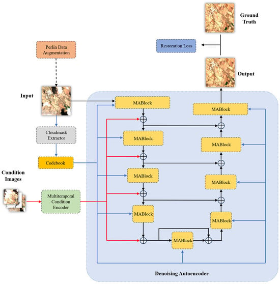
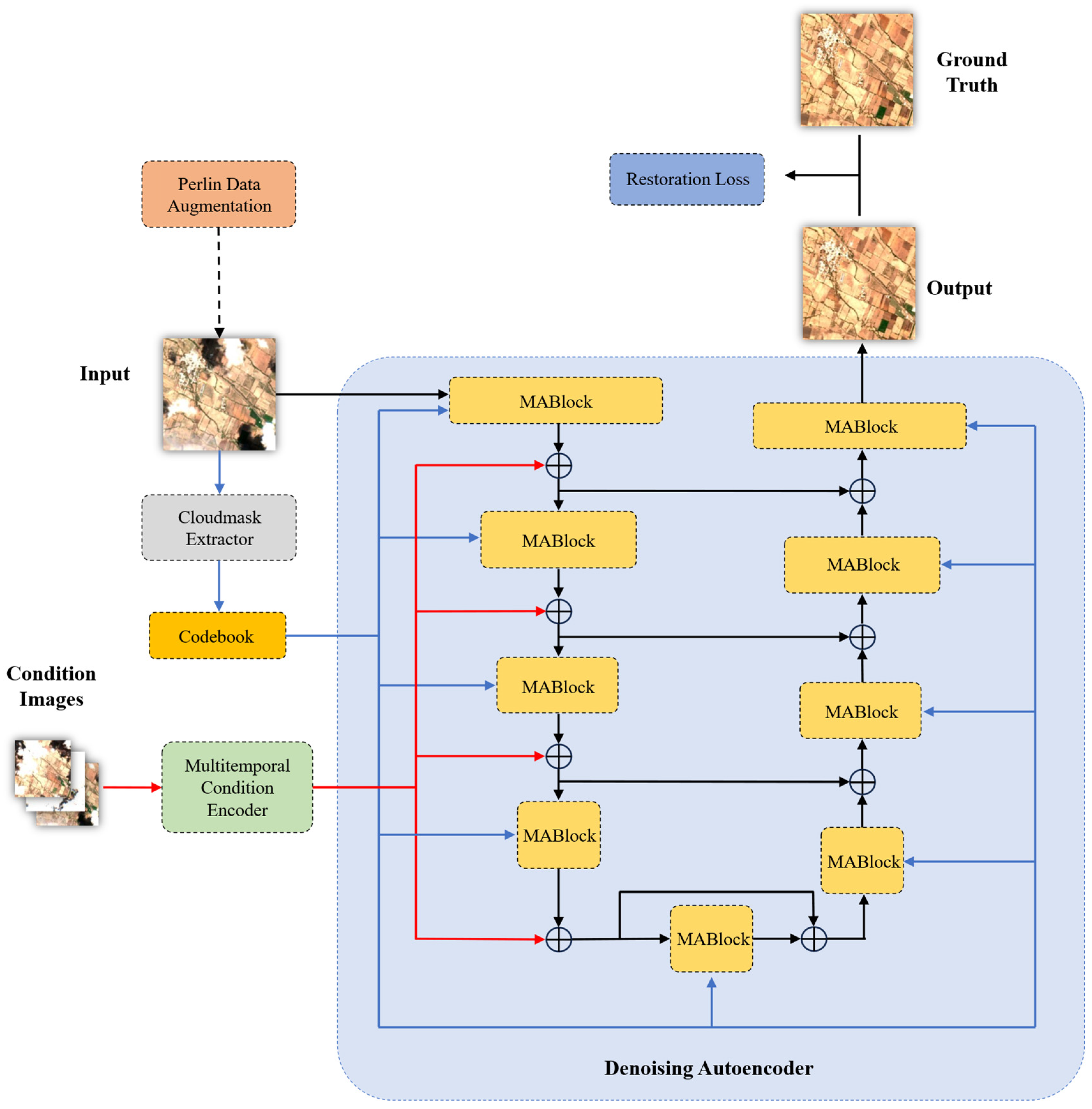
The overall architecture of our proposed PCRDiff is illustrated in Figure 1. Section 2.1 introduces the overall training and iterative denoising process of the model, while Section 2.2 details the structures of the denoising autoencoder, the multi-temporal condition encoder, and the Perlin Noise Quantizer.

Figure 1. The overall structure of Perlin Noise-Based Cloud Removal Diffusion Model (PCRDiff). The model consists of three components: (1) A multi-temporal condition encoder extracts features from the conditional images and provides them as part of the guidance conditions input to the denoising autoencoder. (2) A Perlin Noise Quantizer extracts the cloud mask from the input image and quantizes it into a discrete Perlin noise intensity value via a codebook. This value serves as another part of the guidance conditions and is also used for iterative denoising. (3) The denoising autoencoder takes the input image, conditional images, and the Perlin noise intensity value to predict the final cloud-free image. In the figure, black arrows denote the processing flow of the input image within the model, while the red and black arrows indicate the pathways involving the conditional image and the quantitative value of Perlin noise intensity, respectively. The dashed arrow indicates that Perlin Data Augmentation is optional—specifically, it is applied to 50% of the input data during training.

2.1. Training and Denoising Pipeline

2.1.1. Training Pipeline

The training pipeline of PCRDiff consists of two parts.

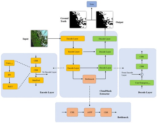
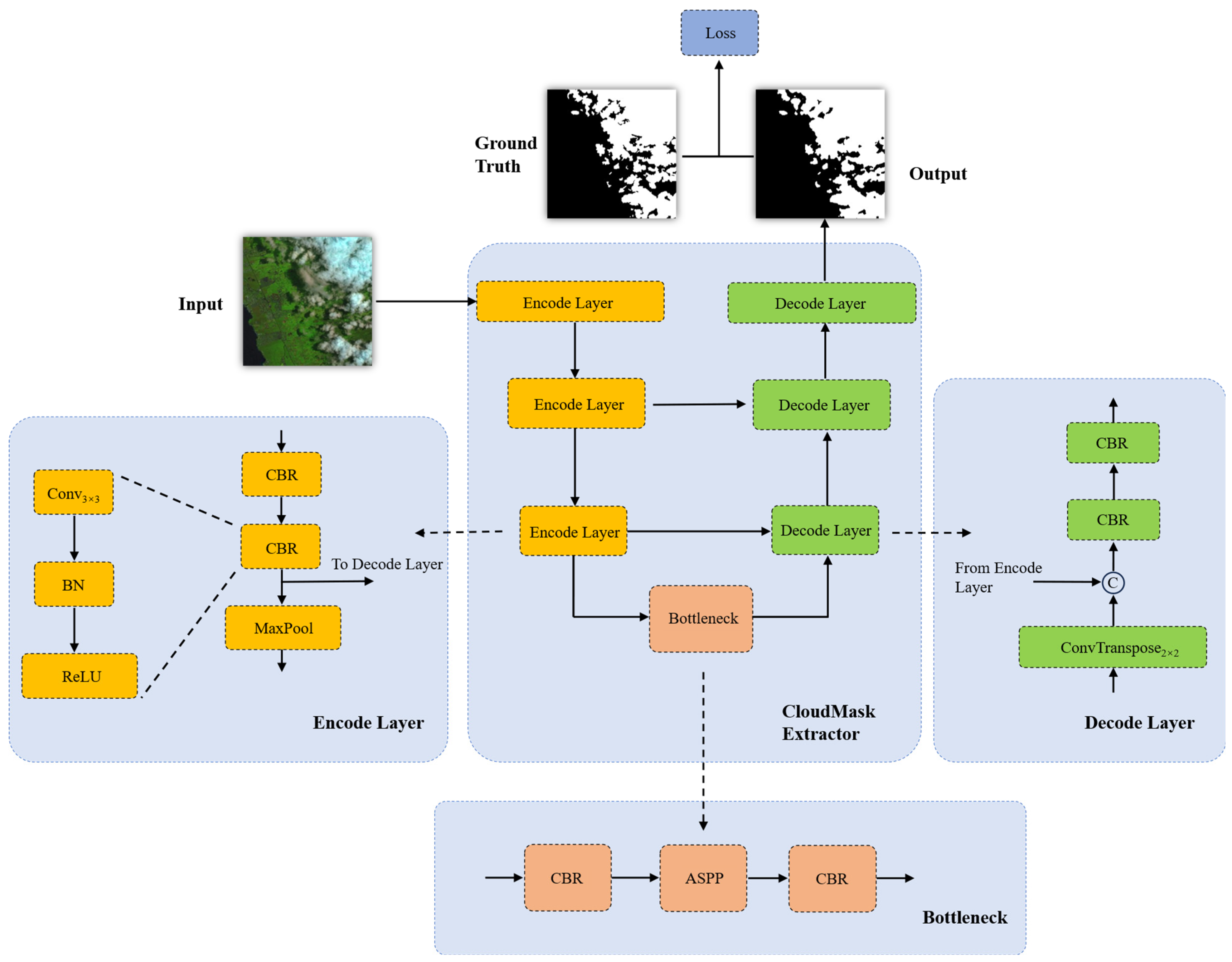
The first part involves training the cloud mask extractor within the Perlin Noise Quantizer. This module is a compact U-Net [39] structure designed to efficiently and rapidly obtain cloud masks from input images. Its architecture is illustrated in Figure 2. It takes a cloudy image as input. In the encoder section, each layer employs a two-layer Convolution-BatchNorm-ReLU (CBR) block to progressively extract features from the input image, followed by a max-pooling layer for downsampling. The bottleneck utilizes an Atrous Spatial Pyramid Pooling (ASPP) [40] structure to further extract features from multiple scales. In the decoder section, each layer uses transposed convolution for upsampling and similarly employs a two-layer CBR block to integrate information from both the bottleneck and the corresponding encoder layer. The final output is a binary cloud mask for the image.

$$CBR\left(X\right)=ReLU\left[BN\left({Conv}_{3\times 3}\left(X\right)\right)\right]$$

(4)

$$EncodeLayer:X_{out}={MaxPool}_{2\times 2}\left[CBR\left(CBR\left(X_{in}\right)\right)\right]$$

(5)

$$DecodeLayer:X_{out}=CBR\left[CBR\right(Concat\left({ConvTranspose}_{2\times 2}\left(X_{in}\right),X_{fromencoder}\right)]$$

(6)

$$Bottleneck:X_{out}=CBR\left[ASPP\left(CBR\left(X_{in}\right)\right)\right]$$

(7)

Figure 2. Architecture Diagram of the Cloudmask Extractor. The dashed line indicates the internal structure of the module.

We compute the loss using a combination of Binary Cross-Entropy loss (BCELoss) and Dice loss [41]:

$$L=BCELoss\left(X_{out},X_{GT}\right)+\lambda ·DiceLoss(X_{out},X_{GT})$$

(8)

where λ is used to control the weighting between the two losses.

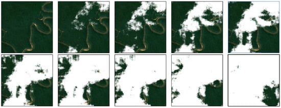
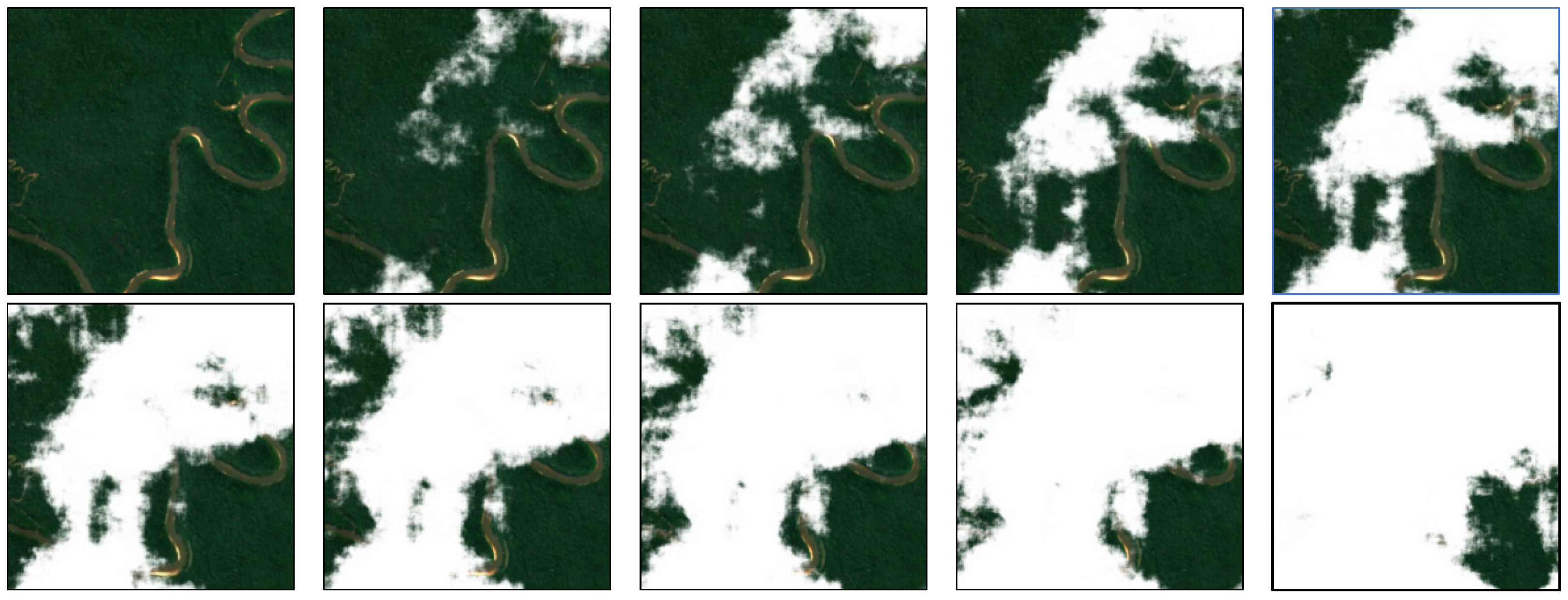
After training the Cloudmask Extractor, the second part involves training the overall model (with the weights of the Cloudmask Extractor module frozen). First, we simulate the interference of cloud occlusion by progressively adding Perlin noise to a cloud-free image using the following method (Algorithm 1):

Algorithm 1: Progressively Adding Perlin Noise to Images

Input: Cloud-free image $X_{in}$ (pre-normalized to the range [−1, 1]) Output: A sequence of images $X_{list}$ with Perlin noise added. $N\left(x,y\right)=PerlinNoise2D\left(x\cdot s,y\cdot s,octaves,persistence,lacunarity\right)$                                              ▷Perlin Noise Base Texture, implemented using the Python noise library $C(x,y)={\displaystyle \frac{1}{2}}[1+N(x,y\left)\right]$   ▷Scale the texture values to the range [0, 1] $S\left(x,e_0,e_1\right)=S\left({\displaystyle \frac{x-e_0}{e_1-e_0}}\right)=S\left(y\right)=\left\{\begin{array}{c}\begin{array}{cc}0& ify\le 0\end{array}\\ \begin{array}{cc}3y^2-2y^3& if0<y\le 1\end{array}\\ \begin{array}{cc}1& ify>1\end{array}\end{array}\right.$   ▷Smoothing Function Init $X_{list}$ as empty list for $\mathrm{k}\in \{1,2,\dots ,\mathrm{N}\}$ do          ${\mathrm{t}}_{\mathrm{k}}={\left({\mathrm{w}}_1·\mathrm{k}\right)}^{{\mathrm{w}}_2}/{\mathrm{w}}_3$   ▷Image Synthesis Control Sequence          $\theta \left(t_k\right)=1-a·t_k,w\left(t_k\right)=b\cdot (1-c{·t}_k)$   ▷Control the cloud coverage speed and edge transition          $M(x,y,t_k)=S\left(C\right(x,y),\theta \left(t_k\right)-w\left(t_k\right),\theta \left(t_k\right)+w\left(t_k\right))$   ▷Cloud Occlusion Mask Sequence          $X_k=[1-M(x,y,t_k\left)\right]\cdot X_{in}(x,y)+M(x,y,t_k)\cdot X_{cloud}$   ▷Final Cloud-Occluded Image Sequence           append $X_k$ to $X_{list}$ end for return $X_{list}$

where $X_{cloud}$ represents the cloud color, s is the scaling factor controlling the noise frequency, octaves is the number of superimposed noise layers, persistence is the intensity attenuation factor between adjacent noise layers, lacunarity is the frequency multiplier between adjacent noise layers, N is the total number of generated image sequences, and ${\mathrm{w}}_1$, ${\mathrm{w}}_2$, ${\mathrm{w}}_3$, a, b, c are hyperparameters in the image generation process. Taking $X_{cloud}$ = (1, 1, 1) (corresponding to (255, 255, 255) in practice), s = 0.005, octaves = 8, persistence = 0.6, lacunarity = 2.0, ${\mathrm{w}}_1$ = 4.5 × 10⁻⁴, ${\mathrm{w}}_2$ = 0.2, ${\mathrm{w}}_3$ = 2, a = 1.2, b = 0.1, c = 0.8, N = 10, as an example, the resulting image sequence we obtained is shown in Figure 3.

Figure 3. Cloud-Occluded Image Sequence Based on Perlin Noise.

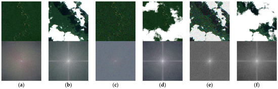
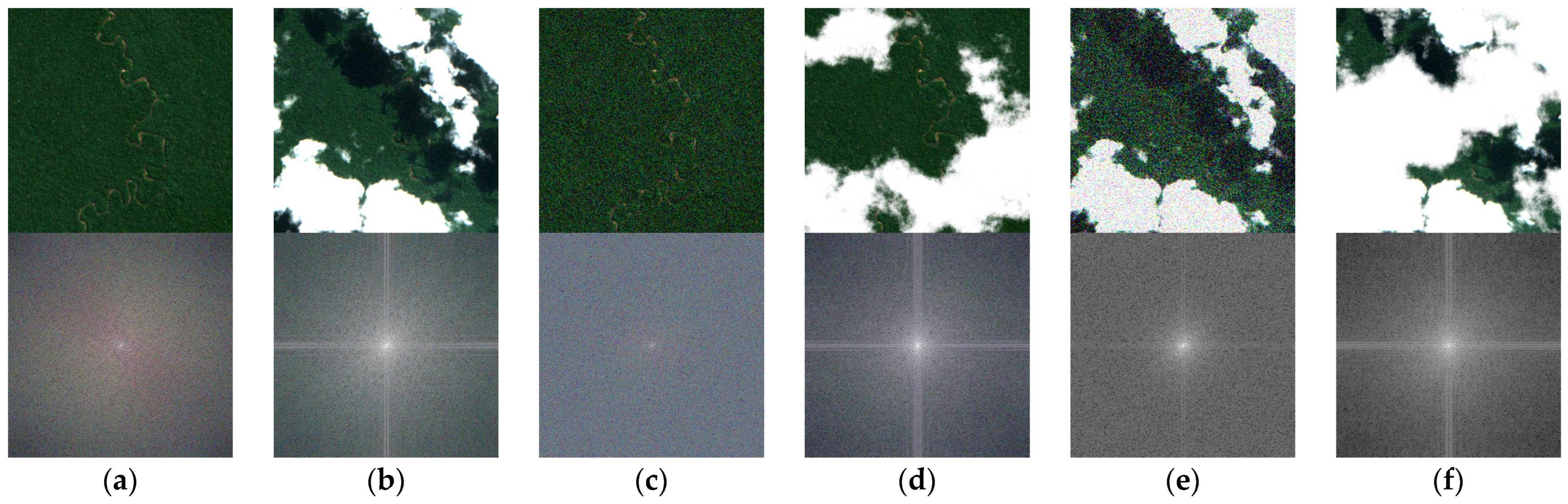
We compared five interference patterns in the frequency domain: cloud occlusion, Gaussian noise, Perlin noise, Gaussian noise combined with cloud occlusion, and Perlin noise combined with cloud occlusion, as shown in Figure 4. The results indicate that, compared to cloud-free images, cloud occlusion in cloudy images introduces distinct horizontal and vertical bright stripes in the spectrograms. Notably, this spectral feature is also present in both cloud-free and cloudy images affected by Perlin noise. In contrast, it is completely absent in cloud-free images corrupted by Gaussian noise and is significantly attenuated in cloudy images affected by Gaussian noise. Therefore, employing Perlin noise as a synthetic perturbation allows for a more accurate simulation of the interference caused by cloud occlusion in cloudy images, enabling the model to learn more effectively how to restore images based on real cloud features. Since a purely frequency-domain analysis is insufficient to determine whether Perlin noise addition on cloud-free or cloudy images yields superior results, we conducted further investigation in the ablation studies section.

Figure 4. Six images and their corresponding frequency spectrograms. (a) is the original cloud-free image, (b) is the original cloudy image, (c) is the cloud-free image corrupted by Gaussian noise, (d) is the cloud-free image corrupted by Perlin noise (the usage of Perlin noise is described in Algorithm 1), (e) is the cloudy image corrupted by Gaussian noise, and (f) is the cloudy image corrupted by Perlin noise. These spectrograms indicate that the interference patterns most closely resembling the cloud occlusion are the interference pattern of Perlin noise and the one formed by the combined effect of Perlin noise and the cloud occlusion.

We define the above process as $D\left(·\right)$, $X_0$ is the cloud-free image and $k$ is a random Perlin noise intensity value. The generated image $X_k$ serves as the input image for the model.

$$X_k=D\left(X_0,k\right)$$

(9)

To achieve single-step cloud removal, our objective is to directly restore a cloud-free image from the cloud-occluded image under the guidance of conditions, namely:

$${\widehat{X}}_0=R_{\theta }(X_k,c,k)$$

(10)

where $c$ represents the conditional cloudy image, and $R_{\theta }\left(·\right)$ is the restoration model with parameters $\theta$. Assuming the model is fully trained, during testing, we obviously cannot directly obtain the original cloud-free image, meaning we cannot get $X_k$ as input via $D\left(X_0,k\right)$. Furthermore, this noise-adding process ultimately produces an image close to pure white. If we mimic traditional diffusion models by starting from pure white noise (or a pure white image) for restoration, it would significantly increase the model’s difficulty in reconstructing the main structure of the image. Therefore, during actual training and inferencing, we choose to treat existing cloudy images as $X_k$ obtained through degradation operation $D\left(X_0,k\right)$ and use them as input images.

To enhance the model’s robustness, we apply Algorithm 1 to a portion of the training data. For each training sample, a Perlin noise intensity value is randomly selected, and a synthetically generated cloudy image processed by Algorithm 1 is returned. We refer to this technique as Perlin Data Augmentation. During the actual training process, we randomly apply Perlin Data Augmentation to 50% of the training data to achieve the goal of increasing data diversity.

During inference, we also use the existing cloudy image as the input. The corresponding Perlin noise intensity value for the input image can be obtained from the Perlin Noise Quantizer (details in Section 3.2). We compute the loss using a combination of Mean Squared Error Loss (MSELoss) and Structural Similarity Index loss (SSIMLoss) [42]:

$$L=MSELoss({\widehat{X}}_0,X_{gt})+\mu ·SSIMLoss({\widehat{X}}_0,X_{gt})$$

(11)

where $X_{gt}$ is the ground truth cloud-free image, and μ is a hyperparameter controlling the weight between the two losses.

2.1.2. Denoising Pipeline

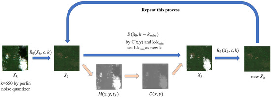
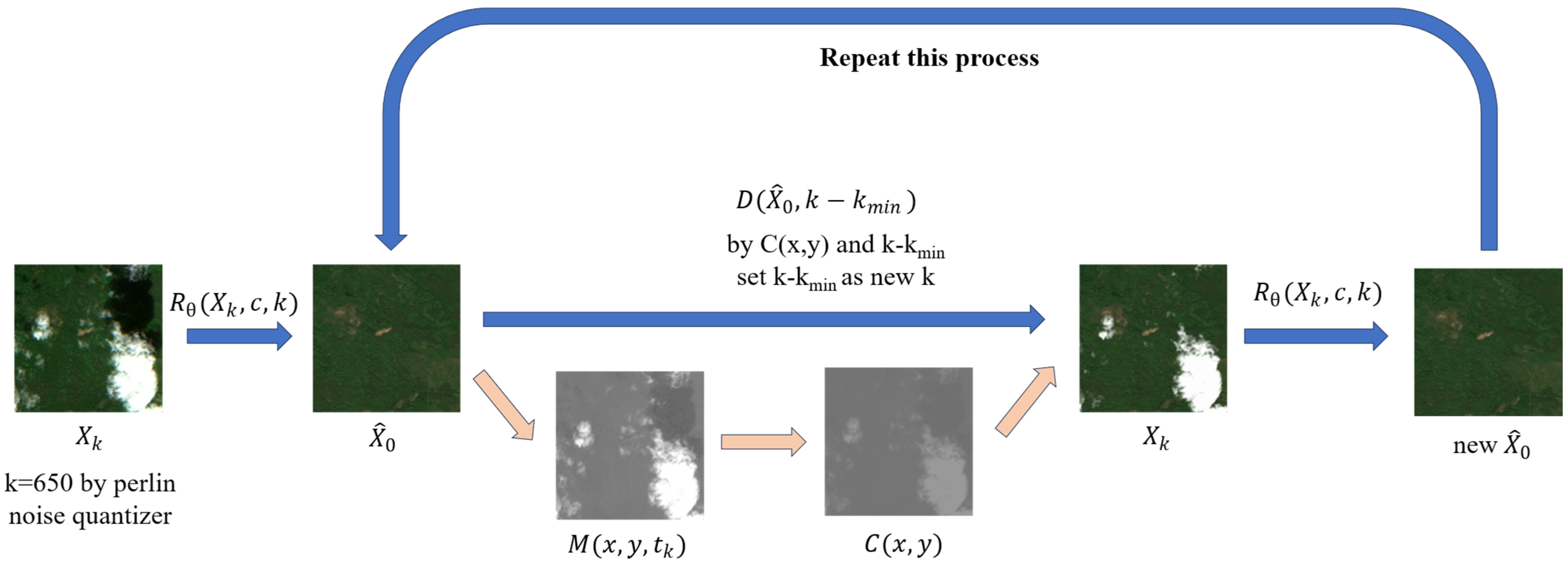
Based on our training pipeline, our model is capable of achieving single-step cloud removal. Additionally, we designed a corresponding inference process that can perform iterative denoising, analogous to traditional diffusion models, as shown in Algorithm 2. Starting from a set of cloudy images, the image with the least cloud occlusion area, selected via the Cloudmask Extractor, is used as the input image. An initial single-step denoised result is obtained via ${\widehat{X}}_0=R_{\theta }(X_k,c,k)$. Subsequently, a feasible $C(x,y)$ that approximately satisfies $X_k=D\left({\widehat{X}}_0,k\right)$ in Algorithm 1 is computed. The degradation process $X_{k-k_{min}}=D\left({\widehat{X}}_0,k-k_{min}\right)$ can then be executed, and the resulting $X_{k-k_{min}}$ is used as the input image for the next denoising step. This process is repeated iteratively. Here, $k_{min}$ is a hyperparameter representing the difference in noise intensity between adjacent denoising steps. The iterative denoising pipeline is illustrated in Figure 5.

Algorithm 2: Iterative Denoising Pipeline

Input: Cloudy images $c_1,c_2,c_3$; Inference steps $step$ Output: Cloud-free image ${\widehat{X}}_0$ $k_1,k_2,k_3=PerlinNoiseQuantizer(c_1,c_2,c_3)$ $k=\mathrm{m}\mathrm{i}\mathrm{n}(k_1,k_2,k_3)$ Select corresponding cloudy image as $X_k$ for $i\in \{1,2,\dots ,\mathrm{s}\mathrm{t}\mathrm{e}\mathrm{p}\}$ do         ${\widehat{X}}_0=R_{\theta }(X_k,c,k)$         if $i<step$ then                 ${\mathrm{t}}_{\mathrm{k}}={\left({\mathrm{w}}_1·\mathrm{k}\right)}^{{\mathrm{w}}_2}/{\mathrm{w}}_3$                 $M\left(x,y,t_k\right)=average({(X}_k-{\widehat{X}}_0)/(X_{cloud}-{\widehat{X}}_0),dim=1)$                                                                                 ▷Compute the mean across the channel dimension.                                                                                 $X_{cloud}$ is broadcast to the spatial dimensions of ${\widehat{X}}_0$.                 $C\left(x,y\right)=\left(2·M\left(x,y,t_k\right)-1\right)·w\left(t_k\right)+\theta \left(t_k\right)$   ▷For computational convenience, the smooth-                                                                                          ing function is approximated as linear here.                 $X_{k-k_{min}}=D({\widehat{X}}_0,k-k_{min})$  ▷Following Algorithm 1, compute $M(x,y,t_{k-k_{min}})$ and $X_{k{-k}_{min}}$                                                           using $C(x,y)$.                 $k=k-k_{min}$         end if end for return ${\widehat{X}}_0$

Figure 5. Schematic Diagram of the Iterative Denoising Pipeline.

2.2. Model Components

2.2.1. Perlin Noise Quantizer

The Perlin Noise Quantizer consists of two components: the Cloudmask Extractor and the Codebook. The Cloudmask Extractor has been detailed in Section 3.1. We applied Algorithm 1 to add Perlin noise of random intensities to cloud-free images. The synthesized images were then processed by the Cloudmask Extractor to obtain cloud masks, and the number of non-zero elements in each mask was counted. After repeated experiments, a clear and stable correspondence was observed between the Perlin noise intensity and the count of non-zero elements in the cloud mask. Based on this finding, we designed a Codebook to convert the cloud mask into a discrete Perlin noise intensity value, k. The structure of the Codebook is relatively simple. We used Algorithm 1 on the same cloud-free image, and the images were randomly corrupted 20 times. In each corruption iteration, all quantization noise levels were traversed. The cloud masks for these corrupted images were then extracted using the Cloudmask Extractor. For each quantization noise level, the number of pixels with a value of 1 in the cloud mask was counted, and its average value over the 20 runs was calculated. This process established a correspondence between the number of cloud mask pixels (value = 1) and the noise intensity, forming the Codebook. In both training and inference stages, the Cloudmask Extractor is utilized to generate a cloud mask from the input image. This mask is subsequently passed to the Codebook, which outputs the corresponding quantized Perlin noise intensity value. Using this module, we can obtain the k value for both real cloudy images and images enhanced via Perlin Data Augmentation.

After obtaining k, we broadcast it to the batch size dimension and apply sinusoidal positional encoding. This encoded representation is then used as an intermediate input to the Multi-Attention Block (see Section 2.2.2).

2.2.2. Denoising Autoencoder

The Denoising Autoencoder is the primary denoising component of PCRDiff, structured as a U-Net comprising four encoder layers, a bottleneck, and four decoder layers. As shown in Figure 1, each encoder layer, decoder layer, and the bottleneck are constructed using a Multi-Attention Block (MABlock). These blocks take the feature maps from the previous layer, along with other guiding conditions as input, and pass their output to the next layer or produce the final inference result of the model. The entire module is trained under the supervision of the restoration loss.

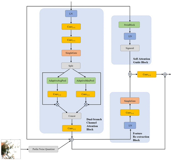
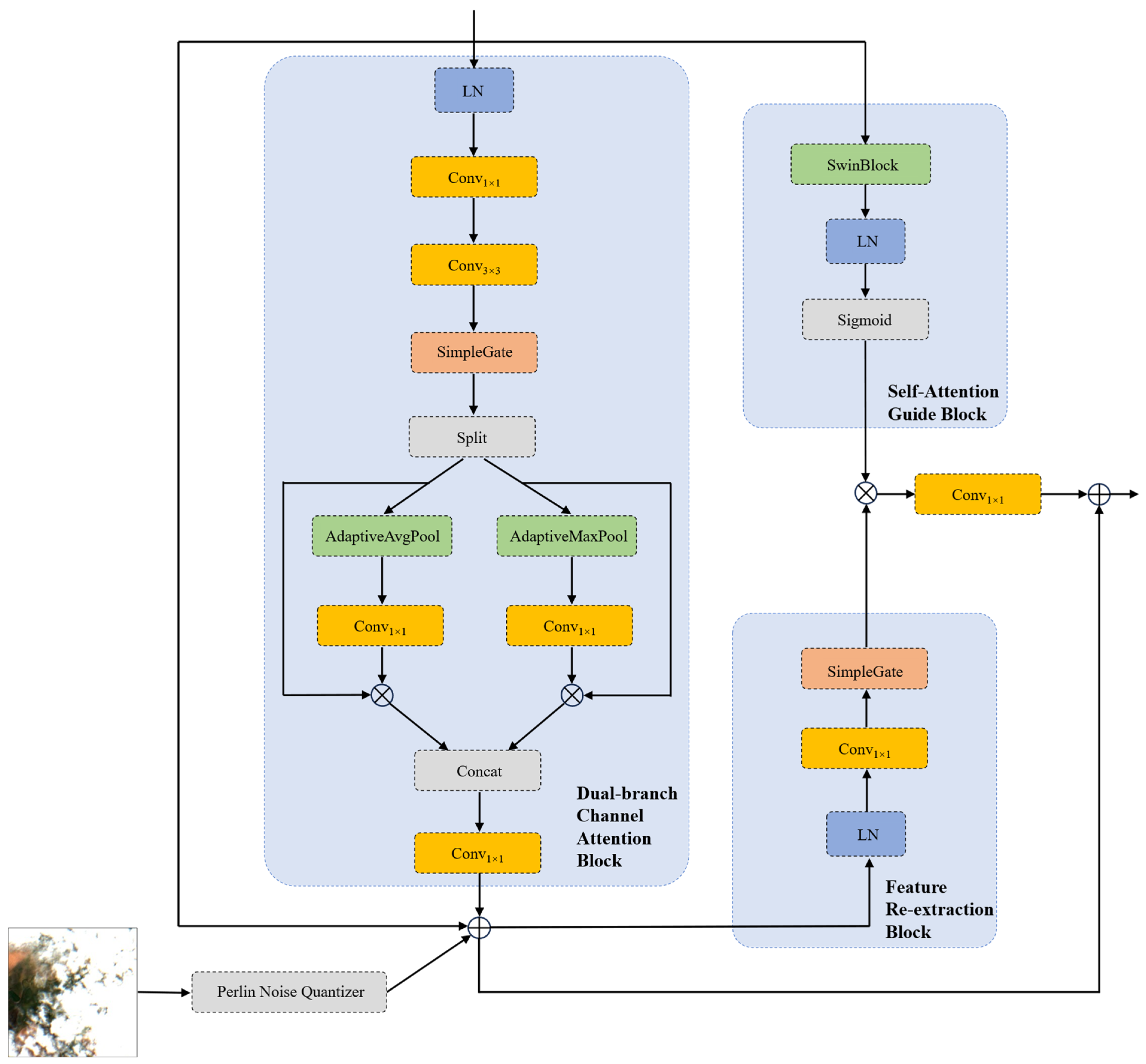
The design of the core architectural blocks significantly impacts model performance. Drawing on design insights from [28,43] and analyzing their limitations, we designed MABlock, illustrated in Figure 6. It integrates both channel attention and self-attention mechanisms, enabling efficient and comprehensive extraction of input image features.

Figure 6. Structure Diagram of the MABlock.

The MABlock consists of three parts: the Dual-branch Channel Attention Block (DCABlock), Feature Re-extraction Block (FRBlock), and the Self-Attention Guide Block (SAGBlock).

$$X_{out}=DCA\left(X_{in}\right)+X_{PNQ}+X_{in}+Conv[SAG\left(X_{in}\right)·FR\left(DCA\left(X_{in}\right)+X_{PNQ}+X_{in}\right)]$$

(12)

where $X_{in}$ is the input feature map, $X_{out}$ is the output feature map, and $X_{PNQ}$ is the Perlin noise intensity encoding input from the Perlin Noise Quantizer.

(1)

Dual-branch Channel Attention Block

The primary purpose of the DCABlock is to extract channel-wise features from the input feature map. First, the input feature map undergoes Layer Normalization to accelerate model convergence. It is then transformed through two convolutional layers before being fed into the SimpleGate structure. The SimpleGate, proposed in [43], is designed to perform the task of a non-linear activation function with relatively low computational complexity. It achieves this by splitting the input feature map into two equal parts along the channel dimension and performing element-wise multiplication.

Subsequently, the feature map is again divided into two equal parts along the channel dimension. One part undergoes Adaptive Max Pooling (AMP) and the other Adaptive Average Pooling (AAP) to extract robust channel features through this dual-branch design. These features are then multiplied by their corresponding halves of the original feature map. Finally, the results from the two branches are concatenated back along the channel dimension, passed through a final convolutional layer, and output as the module’s result.

$$X_a=SimpleGate\left\{{DConv}_{3\times 3}\left[{Conv}_{1\times 1}\left(LN\left(X_{in}\right)\right)\right]\right\}$$

(13)

$$X_{a1},X_{a2}=Split\left(X_a\right)$$

(14)

$$X_{out}={Conv}_{1\times 1}\left\{Concat\left[X_{a1}·{Conv}_{1\times 1}\left(AAP\left(X_{a1}\right)\right),X_{a2}·{Conv}_{1\times 1}\left(AMP\left(X_{a2}\right)\right)\right]\right\}$$

(15)

(2)

Feature Re-extraction Block

The output from the DCABlock is then summed with the Perlin noise intensity encoding provided by the Perlin Noise Quantizer. While this step incorporates noise intensity information, it can also alter the original feature representation. To ensure the features remain robust, we designed a Feature Re-extraction block. This module has a simple structure, consisting only of a Layer Normalization, a convolutional layer, and a SimpleGate.

$$X_{out}=SimpleGate\left[{Conv}_{1\times 1}\left(LN\left(X_{in}\right)\right)\right]$$

(16)

(3)

Self-Attention Guide Block

In the task of remote sensing image cloud removal, input images often contain large cloud-occluded areas, making feature extraction from these regions particularly challenging. The reconstruction of such areas heavily relies on features extracted from more distant, unobstructed regions. However, architectures composed solely of convolutions, normalizations, and pooling operations tend to be confined to extracting and processing local features, often overlooking the global relationships among features within the entire map. This limitation is a key reason why previous methods frequently underperform when restoring large cloud-covered areas. To address this issue, we introduced a self-attention mechanism into the MABlock, namely the Self-Attention Guide block. To reduce computational complexity and improve both training and inference efficiency, we opted not to use a full global Transformer structure. Instead, we employed a Swin Transformer [44] block, which utilizes a shifted window attention mechanism and feature map shifting to achieve an effect approximating global attention while being more computationally efficient. The feature map is processed through the Swin Block, followed by a Layer Normalization and a Sigmoid activation module to prevent gradient vanishing or explosion.

$$X_{out}=Sigmoid\left[LN\left(Swin\left(X_{in}\right)\right)\right]$$

(17)

The output of this module is element-wise multiplied by the output of the Feature Re-extraction block. The result is then integrated through a convolutional layer. Finally, this integrated output is combined with the output of the DCABlock via a residual connection to form the final output of the entire MABlock.

During the encoding phase, the MABlock is followed by a convolutional layer with a stride of 2 for downsampling. During the decoding phase, the MABlock is followed by a convolutional layer with a stride of 1 and a PixelShuffle [45] operation for upsampling.

2.2.3. Multi-Temporal Condition Encoder

The Multi-Temporal Condition Encoder is designed to extract features from multiple cloudy conditional images to guide the model in image reconstruction. Unlike the process of extracting features from the input image being reconstructed, there is no need to consider the internal relationships among features within the conditional images. Therefore, we construct the encoder by removing the SAGBlock from the MABlock. Multiple cloudy images are concatenated along the channel dimension and serve as the input to this module.

2.3. Datasets and Implementation Details

2.3.1. Datasets

During the two-stage model training, we utilized a total of three datasets: SPARCS [46], Sen2_MTC_Old [23], and Sen2_MTC_New [24]. SPARCS selects one scene for each of the 14 major terrestrial habitat types defined by the World Wildlife Fund (WWF), plus scenes for “Inland Waters” and “Rock and Ice” from seven biogeographical realms. Additionally, one extra scene is included for each randomly selected major habitat type, resulting in a total of 80 scenes. The dataset provides detailed mask annotations for clouds, water, ice, land, etc. The images and their corresponding masks have a size of 1000 × 1000 pixels. Sen2_MTC is an image dataset from the Sentinel-2 satellite, consisting of two parts. The Old dataset contains 945 regions from various global locations. Each region has a size of 10,980 × 10,980 pixels with a 10 m resolution and is cropped into multiple 256 × 256 patches. For each geographical location, the clearest image with the lowest cloud coverage is selected as the ground truth label. It is paired with three temporally adjacent cloudy images to form an image set, resulting in a total of 3130 image sets. The New dataset comprises approximately 50 regions. Each region consists of roughly 70 cropped 256 × 256 image pairs. For each geographical location, a set of three cloudy images corresponds to one cloud-free image.

We trained the Cloudmask Extractor using the SPARCS and Sen2_MTC_New datasets. To obtain cloud masks for training, we extracted the cloud-specific segments from the original annotation masks to serve as the ground truth.

For SPARCS, the image and mask sizes differ from those in the Sen2_MTC datasets. Therefore, we pre-processed each image by cropping it into 16 patches of 256 × 256 pixels, with an 8-pixel overlap between adjacent patches in both the width and height dimensions. Patches containing minimal cloud occlusion were filtered out and removed from the training set. The Sen2_MTC_New dataset does not originally provide cloud masks. We generated corresponding cloud masks by binarizing the heatmaps output by CTGAN during its inference phase. Through this process, we obtained a total of 2210 cloud-covered image/cloud mask pairs to form the training dataset for the Cloudmask Extractor.

After completing the training of the Cloudmask Extractor, we froze its parameters and conducted experiments for PCRDiff on the combined Sen2_MTC_Old and Sen2_MTC_New datasets.

2.3.2. Implementation Details

All experiments were conducted on a server running Ubuntu 20.04, equipped with a single NVIDIA RTX 3090 GPU (NVIDIA Corporation, Santa Clara, CA, USA) and 64GB of RAM. The software environment included Python 3.10, PyTorch 1.12, and CUDA 11.8. The Adam optimizer was used for training in both stages. In the training phase for the Cloudmask Extractor, we set the batch size to 8, the initial learning rate to 1 × 10⁻⁴, the weight decay rate to 1 × 10⁻⁴, and trained for a total of 100 epochs. In the training of PCRDiff, we also set the batch size to 8, the initial learning rate to 5 × 10⁻⁵, the weight decay to 0, and trained for a total of 300 epochs. Exponential Moving Average (EMA) [47] was applied during the model training process, updated with a decay rate of 0.9999 after each training iteration, which helps improve the model’s robustness and leads to better performance in testing. We set the hyperparameters for Algorithms 1 and 2 in Section 3 as follows: $X_{cloud}$ = (1, 1, 1), s = 0.005, octaves = 8, persistence = 0.6, lacunarity = 2.0, ${\mathrm{w}}_1$ = 4.5 × 10 ⁻⁴, ${\mathrm{w}}_2$ = 0.2, ${\mathrm{w}}_3$ = 2, a = 1.2, b = 0.1, c = 0.8, N = 10, $k_{min}$=50, λ = 1, μ = 0.001. In the codebook of the Perlin Noise Quantizer, we recorded the cloud mask pixel count for every 50 intensity values, resulting in a total of 40 corresponding relationships, which are used for the discrete quantization of Perlin noise intensity values.

3. Results

3.1. Evaluation Metrics

We employed four metrics to evaluate model performance: PSNR [48], SSIM [42], FID [49], and LPIPS [50]. PSNR measures the pixel-level error between the cloud-removed image and the cloud-free ground truth image; a higher value typically indicates better reconstruction accuracy. SSIM assesses the similarity in structural information between two images, aligning more closely with the human visual system’s perception of structural fidelity, though it remains a pixel-based calculation. FID and LPIPS, on the other hand, are based on feature extraction by deep learning models, measuring the differences between images in a deep feature space. They effectively evaluate the perceptual quality of generated images, better matching human visual perception. LPIPS extracts features using a pre-trained deep network and computes the distance in the feature space. FID is a distribution-level metric; instead of evaluating single generated images, it assesses model performance by comparing the overall data distribution between the set of generated images and the set of real images. It uses intermediate layers of a pre-trained network to extract features from both the generated and real image sets, obtaining two feature matrices, computes their means and covariances, and then derives the final metric value.

3.2. Ablation Studies

We conducted extensive ablation studies to investigate the contribution of the methods, modules and parameters proposed in this paper to PCRDiff. All ablation experiments were performed using the Sen2_MTC_New dataset. The experimental results are presented in Table 1 and Table 2.

Table 1. Quantitative comparison and ablation studies of different modules, methods and parameters, where the optimal and suboptimal metrics are indicated in bold and underline, respectively. The configuration achieving the optimal metrics is highlighted in green.

Modules	Noise Addition Methods	Cloud Mask Acquisition Methods	Perlin Data Augmentation	Number of Quantization Levels	Number of Conditional Images	Noise Frequency (Value of Scale)	PSNR↑	SSIM↑	FID↓	LPIPS↓
Resnet [51]	Gaussian Noise	——	w/o	——	3	——	18.966	0.664	90.542	0.300
NAFBlock [43]	Gaussian Noise	——	w/o	——	3	——	19.042	0.671	83.689	0.295
TCFBlock [28]	Gaussian Noise	——	w/o	——	3	——	19.150	0.671	83.162	0.291
MABlock (ours)	Gaussian Noise	——	w/o	——	3	——	20.244	0.696	78.533	0.284
MABlock (ours)	Perlin Noise	Threshold Segmentation	w/o	40	3	0.005	20.826	0.709	75.633	0.280
MABlock (ours)	Perlin Noise	Cloudmask Extractor	w/o	40	3	0.005	20.902	0.711	74.657	0.278
MABlock (ours)	Perlin Noise	Cloudmask Extractor	Cloud-free	40	3	0.005	20.889	0.710	74.821	0.280
MABlock (ours)	Perlin Noise	Cloudmask Extractor	Cloudy	40	3	0.005	20.988	0.717	72.175	0.273
MABlock (ours)	Perlin Noise	Cloudmask Extractor	Cloudy	80	3	0.005	21.023	0.718	71.392	0.271
MABlock (ours)	Perlin Noise	Cloudmask Extractor	Cloudy	200	3	0.005	21.057	0.720	70.495	0.266
MABlock (ours)	Perlin Noise	Cloudmask Extractor	Cloudy	400	3	0.005	21.049	0.719	70.492	0.267
MABlock (ours)	Perlin Noise	Cloudmask Extractor	Cloudy	200	2	0.005	18.573	0.613	96.390	0.351
MABlock (ours)	Perlin Noise	Cloudmask Extractor	Cloudy	200	1	0.005	15.823	0.504	124.253	0.448
MABlock (ours)	Perlin Noise	Cloudmask Extractor	Cloudy	200	3	0.01	21.021	0.717	72.620	0.271
MABlock (ours)	Perlin Noise	Cloudmask Extractor	Cloudy	200	3	0.003	21.016	0.716	72.409	0.271
MABlock (ours)	Perlin Noise	Cloudmask Extractor	Cloudy	200	3	0.001	20.997	0.712	73.876	0.279

Table 2. Analysis of the denoising steps with the optimal configuration (highlighted in green) in Table 1, where the optimal and suboptimal metrics are indicated in bold and underline, respectively.

Denoising Steps	1	2	3	5	10	20	50	100
PSNR↑	21.057	21.071	21.070	21.076	21.072	21.124	21.123	21.123
SSIM↑	0.720	0.720	0.719	0.719	0.719	0.720	0.720	0.720
FID↓	70.495	70.263	70.246	70.249	70.404	71.028	70.973	70.983
LPIPS↓	0.266	0.266	0.266	0.266	0.266	0.269	0.269	0.269

3.2.1. Modules

We compared the performance of the main U-Net backbone using different modules. In contrast to the previous module types, the most significant difference in the MABlock is the introduction of a self-attention mechanism. Experiments show that, while keeping the overall U-Net structure unchanged (four encoder layers, one bottleneck layer, and four decoder layers), using the MABlock as the core component for the encoder, decoder, and bottleneck layers can significantly improve the model’s performance. This validates the effectiveness of incorporating the self-attention mechanism and the suitability of the MABlock as a core module.

3.2.2. Noise Addition Methods

Conventional diffusion model-based methods typically employ Gaussian noise as a form of corruption. During training, the input is usually a corrupted image formed by adding Gaussian noise to a cloud-free image. During inference, a randomly sampled pure Gaussian noise is often used as the starting point for the denoising process. In contrast, tailored to the characteristics of the remote sensing image cloud removal task, we designed a training pipeline based on Perlin noise. It utilizes existing cloudy images as the input for both training and inference and directs the model to output the cloud-free image directly. The results demonstrate that this training and inference paradigm is highly compatible with the cloud removal task. We attribute this improvement to the physical alignment between the degradation process and the actual cloud occlusion: Perlin noise introduces structured, spatially correlated perturbations that more closely resemble real cloud patterns, enabling the model to learn a restoration mapping that generalizes better to real-world cloudy images. This is further supported by the frequency-domain analysis in Figure 4.

3.2.3. Cloud Mask Acquisition Methods

We experimented with two methods for obtaining cloud masks: threshold segmentation and the Cloudmask Extractor. The results indicate that using the Cloudmask Extractor yields superior performance. We hypothesize that the reason is that in some images, the minimum pixel values within cloud layers can be lower than the higher pixel values in certain ground backgrounds. This makes it impossible to accurately extract cloud information using simple pixel threshold segmentation, regardless of the threshold set. Furthermore, if threshold segmentation is used, the optimal threshold varies across different images. Applying a uniform threshold to all images also leads to suboptimal results. In contrast, the U-Net-based Cloudmask Extractor effectively avoids these issues.

3.2.4. Perlin Data Augmentation

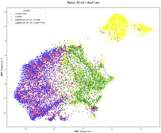
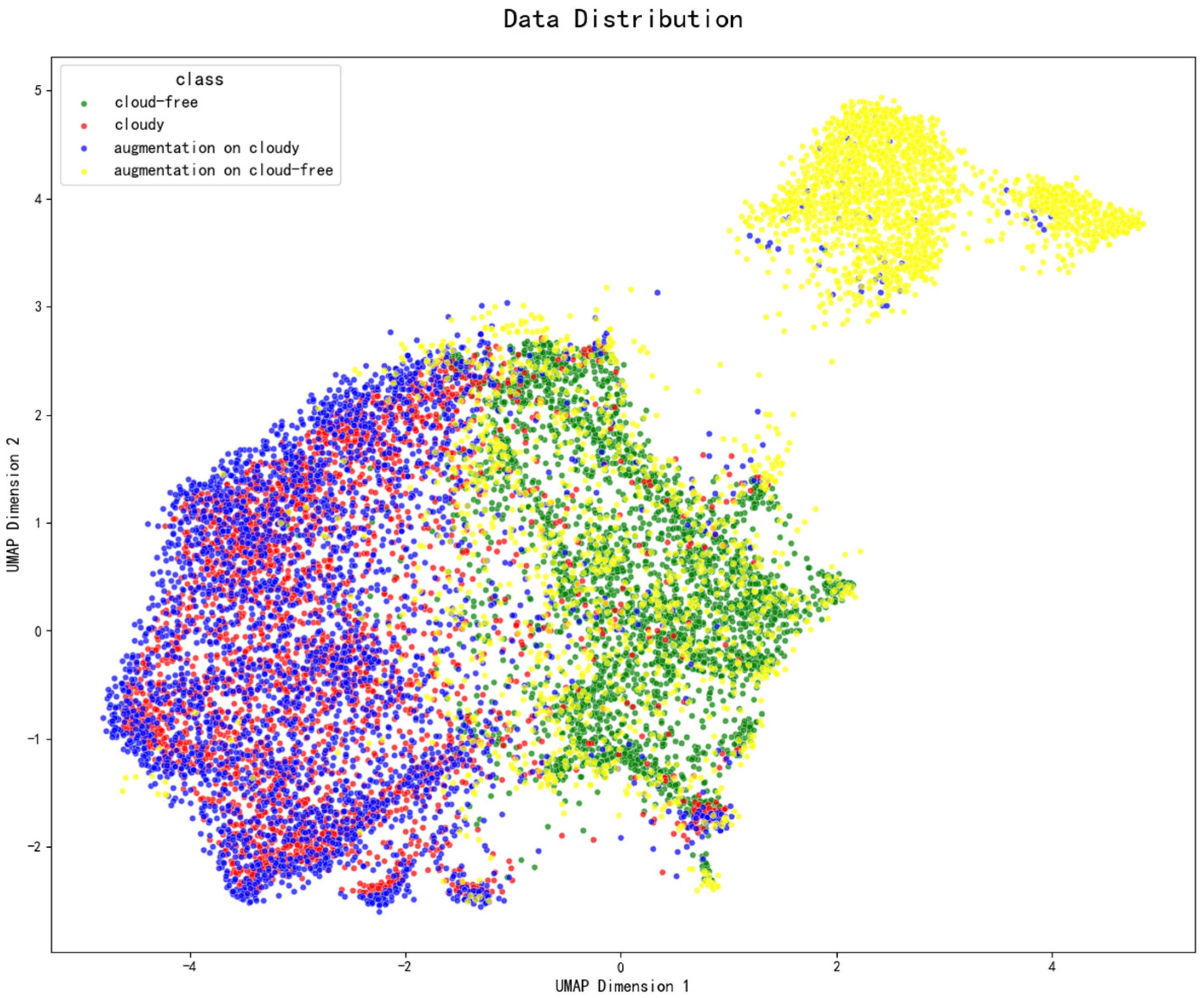
In Algorithm 1, we proposed a noise addition method based on Perlin noise and extended it as Perlin Data Augmentation. We designed two pathways for Perlin Image augmentation, applying it to cloud-free images and to the original cloudy images, respectively. For all cloud-free images in the dataset, we selected a corresponding cloudy image. We applied Perlin Data Augmentation with random intensity to both these cloud-free and cloudy images. This resulted in a total of 3,417 quadruplets, each consisting of: a cloud-free image, a cloudy image, a synthetically enhanced image derived from the cloud-free image, and a synthetically enhanced image derived from the original cloudy image. Subsequently, we used a pre-trained ResNet-50 [52] to extract features and employed UMAP [53] to plot a two-dimensional data distribution, as shown in Figure 7.

Figure 7. Data distribution of the four image categories visualized by UMAP using features extracted by ResNet-50.

As can be seen from the figure, the red scatter points representing the original cloudy images and the blue scatter points representing the synthetically enhanced images derived from cloudy images share an almost identical data distribution. Both are distinctly separated from the green scatter points representing the cloud-free images, forming a clear inter-class distance. This indicates that applying Perlin Data Augmentation to existing cloudy images increases data diversity without altering the original data distribution, thereby not interfering with the model’s learning process. In contrast, the yellow scatter points representing the synthetically enhanced images derived from cloud-free images form a noticeable inter-class distance from the original cloudy images, effectively constituting a third category of images distinct from both cloud-free and original cloudy images. This discrepancy would interfere with the model’s learning process. This explains the results in Table 1: compared to using no Perlin Data Augmentation, applying Perlin Data Augmentation based on cloudy images improves model performance, while using it based on cloud-free images actually degrades performance. This finding aligns with our intuitive understanding: using original cloudy images for data augmentation better preserves the consistency of the enhanced images’ data distribution with that of the original dataset.

3.2.5. Number of Quantization Levels

We compared the performance of the Perlin noise quantizer under varying numbers of quantization levels. Experimental results indicate that when the number of quantization levels is below 200, increasing the number of levels enables more precise quantization of Perlin noise intensity in the input image, thereby enhancing model performance. In contrast, when the number of quantization levels exceeds 200, further refinement of quantization yields marginal improvements, with model performance at 400 quantization levels being nearly identical to that at 200 levels.

3.2.6. Number of Conditional Images

We investigated the impact of varying the number of conditional images on model performance. As expected, increasing the number of conditional images enables the model to leverage more available information for cloud-free image reconstruction, resulting in a substantial improvement in performance. Experimental results demonstrate the effectiveness of the multi-temporal design and its significant contribution to model performance.

3.2.7. Noise Frequency

We investigated the influence of Perlin noise frequency on model performance by varying the scale parameter in Algorithm 1. Experimental results indicate that the optimal performance is achieved when the scale is set to 0.005, with either higher or lower values leading to degraded performance. This suggests that a scale of 0.005 enables Perlin noise to more accurately simulate the interference patterns of real cloud cover.

3.2.8. Denoising Steps

Building upon the previously proposed Perlin noise-based corruption process, we designed a corresponding iterative denoising pipeline. Experiments demonstrate that our model can achieve high-fidelity results with just a single denoising step. As the number of denoising steps increases, PSNR reaches its maximum value (21.124) at step = 20, after which it gradually decreases. SSIM remains consistently stable throughout the increase in denoising steps. FID achieves its minimum value (70.246) at step = 3 and then gradually increases. LPIPS remains stable when step ≤ 10 and increases when step ≥ 20. This indicates that initially increasing the number of denoising steps is beneficial for improving the perceptual quality of the reconstructed image. However, beyond a certain point, further increases lead to over-denoising, causing the evaluation metrics to deteriorate. Consequently, for subsequent comparative experiments with other methods, we selected the result obtained from 1-step denoising.

3.3. Comparison with Other Methods

We compared PCRDiff with several existing methods—including MCGAN [54], STNet [26], DSen2-CR [55], STGAN [23], CTGAN [24], PMAA [27], UnCRtainTS [56], DDPM-CR [57], DiffCR [28] and EMRDM [58]—on both the Sen2_MTC_Old and Sen2_MTC_New datasets. The results of the comparative experiments are presented in Table 3.

Table 3. The result of comparative experiments between our method and other existing methods on two benchmark datasets. The optimal and suboptimal metrics are indicated in bold and underline, respectively.

Methods	Sen2_MTC-Old				Sen2_MTC_New				Params	MACs
	PSNR↑	SSIM↑	FID↓	LPIPS↓	PSNR↑	SSIM↑	FID↓	LPIPS↓	(M)	(G)
MCGAN	21.146	0.481	166.804	0.477	17.448	0.513	147.057	0.447	4.42	71.56
STNet	26.321	0.834	146.057	0.438	16.206	0.427	161.683	0.503	4.64	304.31
DSen2-CR	26.967	0.855	123.382	0.330	16.827	0.534	140.208	0.446	18.92	1240.23
STGAN	26.186	0.734	150.562	0.388	18.152	0.587	182.150	0.513	231.93	1094.94
CTGAN	26.264	0.808	192.270	0.472	18.308	0.609	128.704	0.384	642.92	632.05
PMAA	27.377	0.861	120.393	0.367	18.369	0.614	118.214	0.392	3.45	92.34
UnCRtainTS	26.417	0.837	130.875	0.400	18.770	0.631	93.509	0.333	0.56	37.16
DDPM-CR	27.060	0.854	110.919	0.320	18.742	0.614	94.401	0.329	445.44	852.37
DiffCR	27.109	0.833	113.320	0.349	19.150	0.671	83.162	0.291	22.91	45.86
EMRDM	25.883	0.828	86.928	0.297	20.033	0.688	67.809	0.256	148.88	74.39
Ours	28.037	0.855	80.522	0.281	21.057	0.720	70.495	0.266	106.82	162.88

As shown in the table, our model achieves the best overall performance across eight metrics on two datasets. Specifically, it attains the best results on five metrics (PSNR, FID, LPIPS on the Sen2_MTC_Old dataset, and PSNR, SSIM on the Sen2_MTC_New dataset), with only a slight lag on the SSIM metric for the Sen2_MTC_Old dataset (0.855 vs. 0.861 for PMAA) and on the FID and LPIPS metrics for the Sen2_MTC_New dataset (70.495 and 0.266, respectively, vs. 67.809 and 0.256 for EMRDM). The quantitative comparison results demonstrate that our model achieves the best comprehensive performance in remote sensing image cloud removal.

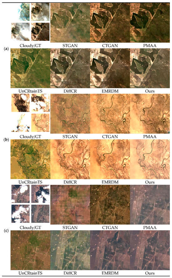
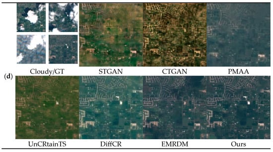
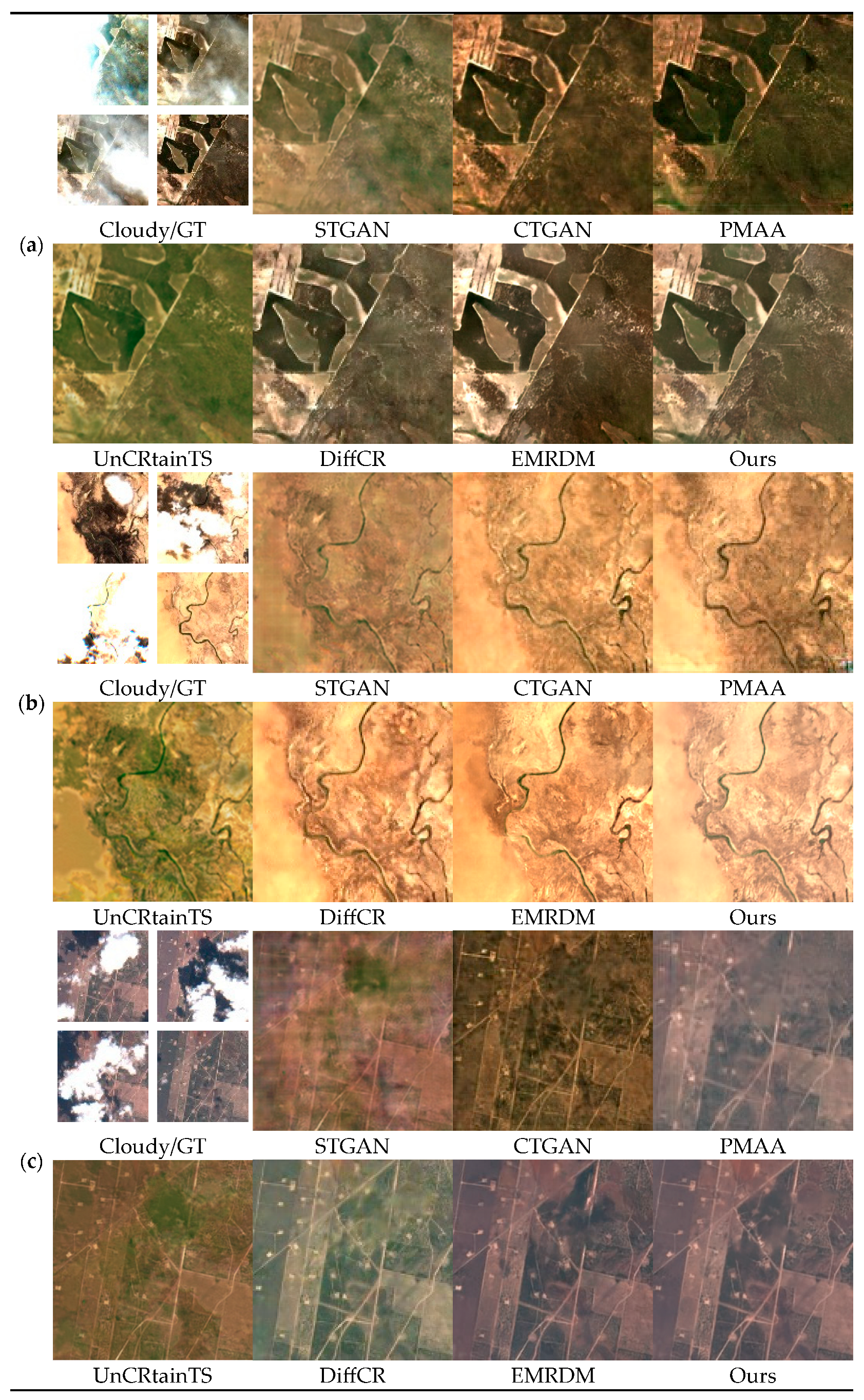
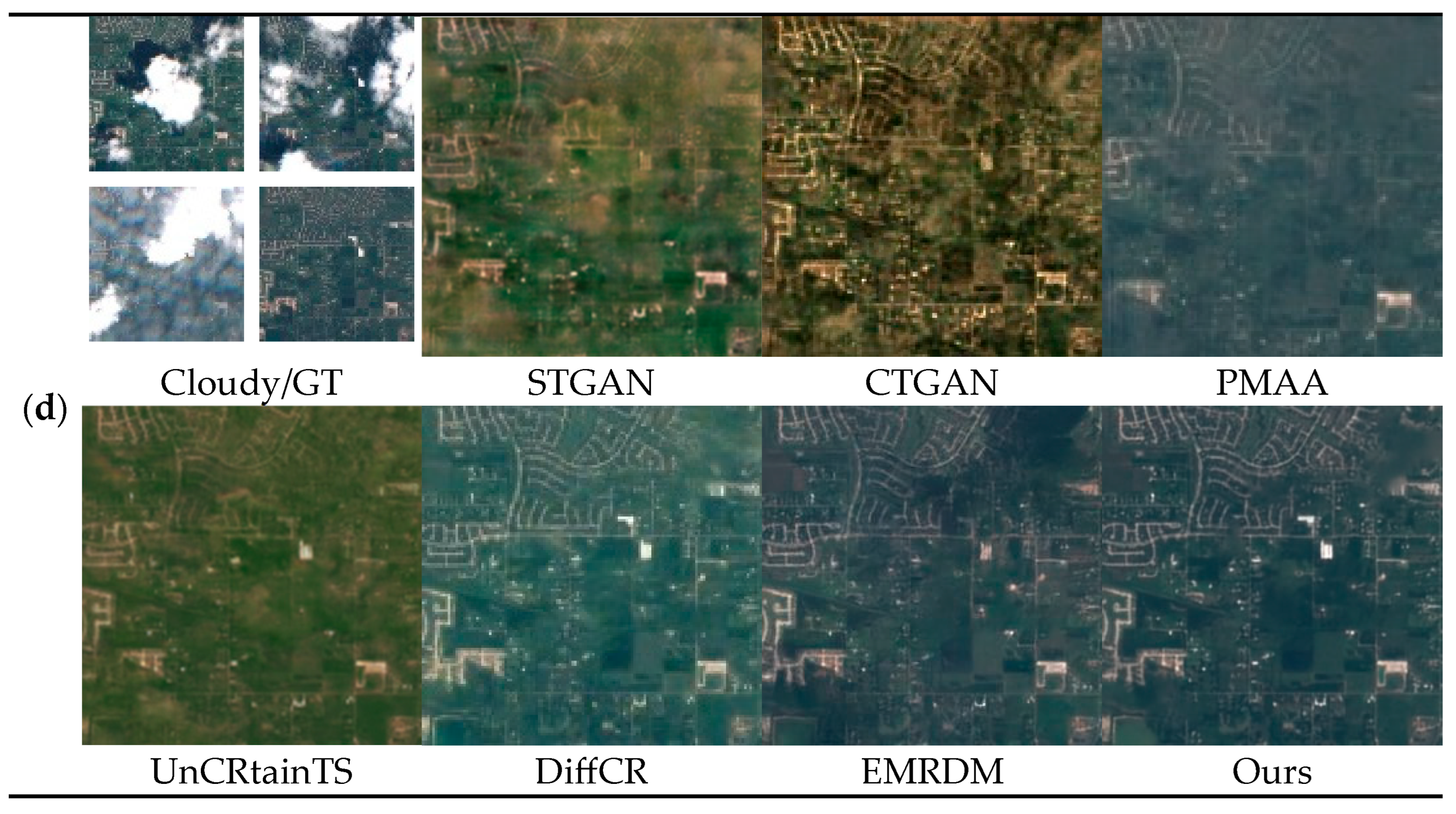
We conducted qualitative experimental comparisons on two datasets simultaneously. Color and texture fidelity present significant challenges in the process of image reconstruction. As shown in Figure 8, compared to other methods, our model not only achieves effective cloud removal but also maximizes color consistency between the restored images and the original ones. Furthermore, it accurately reconstructs textures such as field boundaries, river channels, and streets, thereby producing cloud-free reconstructions with higher fidelity. These comparative experiments demonstrate the effectiveness of the proposed method and its modules. Notably, by leveraging the advantage of achieving high perceptual quality results in a single step, our model attained the aforementioned superior performance while maintaining reasonably moderate model parameters (106.82M) and multiply–accumulate operations (162.88G).

Figure 8. Qualitative comparison between our proposed method and other existing methods. (a,b) show the comparative results on the Sen2_MTC_New dataset, and (c,d) show the comparative results on the Sen2_MTC_Old dataset.

4. Discussion

PCRDiff addresses the inconsistency between the interference pattern of Gaussian noise and that of cloud occlusion when applying diffusion models to remote sensing image cloud removal. It proposes a novel training and inference paradigm, constructs a complete operational pipeline using Perlin noise, and designs corresponding modules for noise intensity extraction, condition extraction, and core cloud removal.

From a workflow perspective, compared to the traditional approach of using Gaussian noise for corruption, our proposed method based on Perlin noise is more aligned with the remote sensing image cloud removal task. Using cloudy images directly as input during both training and inference relieves the model from the burden of reconstructing the main structure of the cloud-free image. Directly predicting the cloud-free outcome enables our model to generate high-fidelity, cloud-free images in a single step. Furthermore, the Perlin Data Augmentation derived from our corruption method effectively increases the diversity of training data and enhances the model’s robustness.

From a module design perspective, our designed Perlin Noise Quantizer efficiently and accurately extracts the equivalent Perlin noise intensity from cloudy images. The Multi-temporal Condition Encoder extracts robust features from reference images. The MABlock, employed as the core component within the main U-Net backbone, leverages multiple attention mechanisms, enabling the model to ultimately generate cloud-free images with high fidelity and perceptual quality.

Experimental results demonstrate that our model achieves superior performance on both benchmark datasets (Sen2_MTC_Old and Sen2_MTC_New), validating the effectiveness of the proposed method and its individual modules.

However, the current research still has limitations: In the stage of applying Perlin noise for corruption, we directly set hyperparameters that appear reasonable manually, but these may not be optimal for this specific model and the cloud removal task. Furthermore, our Perlin Data Augmentation does not account for the effects of cloud shadows, and we employ the same processing approach regardless of the varying thickness of cloud layers, indicating room for improvement in the algorithm’s design.

5. Conclusions

This paper proposes a novel diffusion model, PCRDiff, for remote sensing image cloud removal. Unlike other prevalent models in this domain, PCRDiff employs Perlin noise as the corruption mechanism within its diffusion process. A corresponding training and inference pipeline is designed around this approach, alongside novel feature extraction modules to enhance model performance. Our extensive experiments demonstrate that our method outperforms other approaches in cloud removal, achieving cloud-free image reconstruction with high fidelity and perceptual quality.

In the future, we will further investigate more principled parameter settings and algorithmic designs for the Perlin noise-based corruption process. Additionally, we plan to explore how to integrate other modalities (such as near-infrared or SAR imagery) to improve information utilization and develop even more efficient and accurate remote sensing image cloud removal methods.

References

- Dong, C.; Loy, C.C.; He, K.; Tang, X. Learning a deep convolutional network for image super-resolution. In Proceedings of the European Conference on Computer Vision; Springer: Cham, Switzerland, 2014; pp. 184–199. [Google Scholar]
- Lim, B.; Son, S.; Kim, H.; Nah, S.; Lee, K.M. Enhanced deep residual networks for single image super-resolution. In Proceedings of the IEEE Conference on Computer Vision and Pattern Recognition Workshops, Honolulu, HI, USA, 21–26 July 2017; pp. 136–144. [Google Scholar]
- Ledig, C.; Theis, L.; Huszár, F.; Caballero, J.; Cunningham, A.; Acosta, A.; Aitken, A.; Tejani, A.; Totz, J.; Wang, Z.; et al. Photo-realistic single image super-resolution using a generative adversarial network. In Proceedings of the IEEE Conference on Computer Vision and Pattern Recognition, Honolulu, HI, USA, 21–26 July 2017; pp. 4681–4690. [Google Scholar]
- Lu, Z.; Li, J.; Liu, H.; Huang, C.; Zhang, L.; Zeng, T. Transformer for single image super-resolution. In Proceedings of the IEEE/CVF Conference on Computer Vision and Pattern Recognition, New Orleans, LA, USA, 18–24 June 2022; pp. 457–466. [Google Scholar]
- Kupyn, O.; Budzan, V.; Mykhailych, M.; Mishkin, D.; Matas, J. DeblurGAN: Blind motion deblurring using conditional adversarial networks. In Proceedings of the IEEE Conference on Computer Vision and Pattern Recognition, Salt Lake City, UT, USA, 18–22 June 2018; pp. 8183–8192. [Google Scholar]
- Nah, S.; Hyun Kim, T.; Mu Lee, K. Deep multi-scale convolutional neural network for dynamic scene deblurring. In Proceedings of the IEEE Conference on Computer Vision and Pattern Recognition, Honolulu, HI, USA, 21–26 July 2017; pp. 3883–3891. [Google Scholar]
- Zhao, S.; Zhang, Z.; Hong, R.; Xu, M.; Yang, Y.; Wang, M. FCL-GAN: A lightweight and real-time baseline for unsupervised blind image deblurring. In Proceedings of the 30th ACM International Conference on Multimedia, Lisboa, Portugal, 10–14 October 2022; pp. 6220–6229. [Google Scholar]
- Zhang, K.; Zuo, W.; Chen, Y.; Meng, D.; Zhang, L. Beyond a Gaussian denoiser: Residual learning of deep CNN for image denoising. IEEE Trans. Image Process. 2017, 26, 3142–3155. [Google Scholar] [CrossRef] [Scilit] [PubMed]
- Valsesia, D.; Fracastoro, G.; Magli, E. Deep graph-convolutional image denoising. IEEE Trans. Image Process. 2020, 29, 8226–8237. [Google Scholar] [CrossRef] [Scilit] [PubMed]
- King, M.D.; Platnick, S.; Menzel, W.P.; Ackerman, S.A.; Hubanks, P.A. Spatial and temporal distribution of clouds observed by MODIS onboard the Terra and Aqua satellites. IEEE Trans. Geosci. Remote Sens. 2013, 51, 3826–3852. [Google Scholar] [CrossRef] [Scilit]
- Creswell, A.; White, T.; Dumoulin, V.; Arulkumaran, K.; Sengupta, B.; Bharath, A.A. Generative adversarial networks: An overview. IEEE Signal Process. Mag. 2018, 35, 53–65. [Google Scholar] [CrossRef] [Scilit]
- Sohl-Dickstein, J.; Weiss, E.; Maheswaranathan, N.; Ganguli, S. Deep unsupervised learning using nonequilibrium thermodynamics. In Proceedings of the International Conference on Machine Learning, Lille, France, 6–11 July 2015; pp. 2256–2265. [Google Scholar]
- Ganguly, B.; Bhattacharya, A.; Srivastava, A.; Dey, D.; Munshi, S. Single image haze removal with haze map optimization for various haze concentrations. IEEE Trans. Circuits Syst. Video Technol. 2021, 32, 286–301. [Google Scholar] [CrossRef] [Scilit]
- Song, C.; Xiao, C.; Zhang, Y.; Sui, H. Thin Cloud Removal for Single RGB Aerial Image. In Computer Graphics Forum; Wiley: Hoboken, NJ, USA, 2021; Volume 40, pp. 398–409. [Google Scholar]
- Hsu, W.Y.; Chen, Y. Single image dehazing using wavelet-based hazelines and denoising. IEEE Access 2021, 9, 104547–104559. [Google Scholar] [CrossRef] [Scilit]
- Xu, M.; Jia, X.; Pickering, M.; Jia, S. Thin cloud removal from optical remote sensing images using the noise-adjusted principal components transform. ISPRS J. Photogramm. Remote Sens. 2019, 149, 215–225. [Google Scholar] [CrossRef] [Scilit]
- Pan, H. Cloud removal for remote sensing imagery via spatial attention generative adversarial network. arXiv 2020, arXiv:2009.13015. [Google Scholar] [CrossRef] [Scilit]
- Xu, M.; Deng, F.; Jia, S.; Jia, X.; Plaza, A.J. Attention mechanism-based generative adversarial networks for cloud removal in Landsat images. Remote Sens. Environ. 2022, 271, 112902. [Google Scholar] [CrossRef] [Scilit]
- Zhao, X.; Jia, K. Cloud removal in remote sensing using sequential-based diffusion models. Remote Sens. 2023, 15, 2861. [Google Scholar] [CrossRef] [Scilit]
- Hu, Y.; Lohit, S.; Kamilov, U.S.; Marks, T.K. Multimodal diffusion bridge with attention-based sar fusion for satellite image cloud removal. IEEE Trans. Geosci. Remote Sens. 2025, 63, 5639612. [Google Scholar] [CrossRef] [Scilit]
- Wang, M.; Song, Y.; Wei, P.; Xian, X.; Shi, Y.; Lin, L. IDF-CR: Iterative diffusion process for divide-and-conquer cloud removal in remote-sensing images. IEEE Trans. Geosci. Remote Sens. 2024, 62, 1–14. [Google Scholar] [CrossRef] [Scilit]
- Yu, Z.; Idris, M.Y.I.; Wang, P. DC4CR: When Cloud Removal Meets Diffusion Control in Remote Sensing. arXiv 2025, arXiv:2504.14785. [Google Scholar]
- Sarukkai, V.; Jain, A.; Uzkent, B.; Ermon, S. Cloud removal in satellite images using spatiotemporal generative networks. In Proceedings of the 2020 IEEE Winter Conference on Applications of Computer Vision, Snowmass, CO, USA, 1–5 March 2020; IEEE: New York, NY, USA; pp. 1785–1794. [Google Scholar]
- Huang, G.-L.; Wu, P.-Y. CTGAN: Cloud transformer generative adversarial network. In Proceedings of the 2022 IEEE International Conference on Image Processing (ICIP), Bordeaux, France, 16–19 October 2022; IEEE: New York, NY, USA; pp. 511–515. [Google Scholar]
- Bermudez, J.D.; Happ, P.N.; Oliveira, D.A.B.; Feitosa, R.Q. SAR to optical image synthesis for cloud removal with generative adversarial networks. ISPRS Ann. Photogramm. Remote Sens. Spat. Inf. Sci. 2018, 4, 5–11. [Google Scholar] [CrossRef] [Scilit]
- Chen, Y.; Weng, Q.; Tang, L.; Zhang, X.; Bilal, M.; Li, Q. Thick clouds removing from multitemporal Landsat images using spatiotemporal neural networks. IEEE Trans. Geosci. Remote Sens. 2020, 60, 1–14. [Google Scholar] [CrossRef] [Scilit]
- Zou, X.; Li, K.; Xing, J.; Tao, P.; Cui, Y. PMAA: A progressive multi-scale attention autoencoder model for high-performance cloud removal from multi-temporal satellite imagery. arXiv 2023, arXiv:2303.16565. [Google Scholar]
- Zou, X.; Li, K.; Xing, J.; Zhang, Y.; Wang, S.; Jin, L.; Tao, P. DiffCR: A fast conditional diffusion framework for cloud removal from optical satellite images. IEEE Trans. Geosci. Remote Sens. 2024, 62, 1–14. [Google Scholar] [CrossRef] [Scilit]
- Li, W.; Li, Y.; Chen, D.; Chan, J.C.W. Thin cloud removal with residual symmetrical concatenation network. ISPRS J. Photogramm. Remote Sens. 2019, 153, 137–150. [Google Scholar] [CrossRef] [Scilit]
- Li, C.; Liu, X.; Li, S. Transformer meets GAN: Cloud-free multispectral image reconstruction via multisensor data fusion in satellite images. IEEE Trans. Geosci. Remote Sens. 2023, 61, 1–13. [Google Scholar] [CrossRef] [Scilit]
- Krizhevsky, A.; Sutskever, I.; Hinton, G.E. ImageNet classification with deep convolutional neural networks. Adv. Neural Inf. Process. Syst. 2012, 25, 1097–1105. [Google Scholar] [CrossRef] [Scilit]
- Vaswani, A.; Shazeer, N.; Parmar, N.; Uszkoreit, J.; Jones, L.; Gomez, A.N.; Kaiser, L.; Polosukhin, I. Attention is all you need. Adv. Neural Inf. Process. Syst. 2017, 30, 5998–6008. [Google Scholar]
- Li, X.; Ren, Y.; Jin, X.; Lan, C.; Wang, X.; Zeng, W.; Wang, X.; Chen, Z. Diffusion models for image restoration and enhancement: A comprehensive survey. Int. J. Comput. Vis. 2025, 133, 8078–8108. [Google Scholar] [CrossRef] [Scilit]
- Rombach, R.; Blattmann, A.; Lorenz, D.; Esser, P.; Ommer, B. High-resolution image synthesis with latent diffusion models. In Proceedings of the IEEE/CVF Conference on Computer Vision and Pattern Recognition, New Orleans, LA, USA, 18–24 June 2022; pp. 10684–10695. [Google Scholar]
- Yu, F.; Gu, J.; Li, Z.; Hu, J.; Kong, X.; Wang, X.; He, J.; Qiao, Y.; Dong, C. Scaling up to excellence: Practicing model scaling for photo-realistic image restoration in the wild. In Proceedings of the IEEE/CVF Conference on Computer Vision and Pattern Recognition, Seattle, WA, USA, 17–21 June 2024; pp. 25669–25680. [Google Scholar]
- Singh, S.; Keserwani, P.; Iwamura, M.; Roy, P.P. DCDM: Diffusion-conditioned-diffusion model for scene text image super-resolution. In Proceedings of the European Conference on Computer Vision, Milan, Italy, 29 September–4 October 2024; Springer: Cham, Switzerland, 2024; pp. 303–320. [Google Scholar]
- Ho, J.; Jain, A.; Abbeel, P. Denoising diffusion probabilistic models. Adv. Neural Inf. Process. Syst. 2020, 33, 6840–6851. [Google Scholar]
- Bansal, A.; Borgnia, E.; Chu, H.M.; Li, J.; Kazemi, H.; Huang, F.; Goldblum, M.; Geiping, J.; Goldstein, T. Cold diffusion: Inverting arbitrary image transforms without noise. Adv. Neural Inf. Process. Syst. 2023, 36, 41259–41282. [Google Scholar]
- Ronneberger, O.; Fischer, P.; Brox, T. U-Net: Convolutional networks for biomedical image segmentation. In Proceedings of the International Conference on Medical Image Computing and Computer-Assisted Intervention; Springer: Cham, Switzerland, 2015; pp. 234–241. [Google Scholar]
- Chen, L.C.; Zhu, Y.; Papandreou, G.; Schroff, F.; Adam, H. Encoder-decoder with atrous separable convolution for semantic image segmentation. In Proceedings of the European Conference on Computer Vision, Munich, Germany, 8–14 September 2018; pp. 801–818. [Google Scholar]
- Li, X.; Sun, X.; Meng, Y.; Liang, J.; Wu, F.; Li, J. Dice loss for data-imbalanced NLP tasks. In Proceedings of the 58th Annual Meeting of the Association for Computational Linguistics, Online, 5–10 July 2020; pp. 465–476. [Google Scholar]
- Wang, Z.; Bovik, A.C.; Sheikh, H.R.; Simoncelli, E.P. Image quality assessment: From error visibility to structural similarity. IEEE Trans. Image Process. 2004, 13, 600–612. [Google Scholar] [CrossRef] [Scilit]
- Chen, L.; Chu, X.; Zhang, X.; Sun, J. Simple baselines for image restoration. In Proceedings of the European Conference on Computer Vision; Springer: Cham, Switzerland, 2022; pp. 17–33. [Google Scholar]
- Liu, Z.; Lin, Y.; Cao, Y.; Hu, H.; Wei, Y.; Zhang, Z.; Lin, S.; Guo, B. Swin transformer: Hierarchical vision transformer using shifted windows. In Proceedings of the IEEE/CVF International Conference on Computer Vision, Montreal, QC, Canada, 10–17 October 2021; pp. 10012–10022. [Google Scholar]
- Shi, W.; Caballero, J.; Huszár, F.; Totz, J.; Aikten, A.P.; Bishop, R.; Rueckert, D.; Wang, Z. Real-time single image and video super-resolution using an efficient sub-pixel convolutional neural network. In Proceedings of the IEEE Conference on Computer Vision and Pattern Recognition, Las Vegas, NV, USA, 27–30 June 2016; pp. 1874–1883. [Google Scholar]
- Hughes, M.J.; Kennedy, R. High-quality cloud masking of Landsat 8 imagery using convolutional neural networks. Remote Sens. 2019, 11, 2591. [Google Scholar] [CrossRef] [Scilit]
- Izmailov, P.; Podoprikhin, D.; Garipov, T.; Vetrov, D.; Wilson, A.G. Averaging weights leads to wider optima and better generalization. In Proceedings of the 34th Conference on Uncertainty in Artificial Intelligence, Monterey, CA, USA, 6–10 August 2018; pp. 876–885. [Google Scholar]
- Sheikh, H.R.; Sabir, M.F.; Bovik, A.C. A statistical evaluation of recent full reference image quality assessment algorithms. IEEE Trans. Image Process. 2006, 15, 3440–3451. [Google Scholar] [CrossRef] [Scilit] [PubMed]
- Heusel, M.; Ramsauer, H.; Unterthiner, T.; Nessler, B.; Hochreiter, S. GANs trained by a two time-scale update rule converge to a local Nash equilibrium. Adv. Neural Inf. Process. Syst. 2017, 30, 6629–6640. [Google Scholar]
- Zhang, R.; Isola, P.; Efros, A.A.; Shechtman, E.; Wang, O. The unreasonable effectiveness of deep features as a perceptual metric. In Proceedings of the IEEE Conference on Computer Vision and Pattern Recognition, Salt Lake City, UT, USA, 18–22 June 2018; pp. 586–595. [Google Scholar]
- Saharia, C.; Chan, W.; Chang, H.; Lee, C.; Ho, J.; Salimans, T.; Fleet, D.; Norouzi, M. Palette: Image-to-image diffusion models. In Proceedings of the ACM SIGGRAPH 2022 Conference Proceedings, Vancouver, BC, Canada, 7–11 August 2022; pp. 1–10. [Google Scholar]
- He, K.; Zhang, X.; Ren, S.; Sun, J. Deep residual learning for image recognition. In Proceedings of the IEEE Conference on Computer Vision and Pattern Recognition, Las Vegas, NV, USA, 27–30 June 2016; pp. 770–778. [Google Scholar]
- McInnes, L.; Healy, J.; Melville, J. UMAP: Uniform manifold approximation and projection for dimension reduction. arXiv 2018, arXiv:1802.03426. [Google Scholar]
- Enomoto, K.; Sakurada, K.; Wang, W.; Fukui, H.; Matsuoka, M.; Nakamura, R.; Kawaguchi, N. Filmy cloud removal on satellite imagery with multispectral conditional generative adversarial nets. In Proceedings of the IEEE Conference on Computer Vision and Pattern Recognition Workshops, Honolulu, HI, USA, 21–26 July 2017; pp. 48–56. [Google Scholar]
- Meraner, A.; Ebel, P.; Zhu, X.X.; Schmitt, M. Cloud removal in Sentinel-2 imagery using a deep residual neural network and SAR-optical data fusion. ISPRS J. Photogramm. Remote Sens. 2020, 166, 333–346. [Google Scholar] [CrossRef] [Scilit]
- Ebel, P.; Garnot, V.S.F.; Schmitt, M.; Wegner, J.D.; Zhu, X.X. UnCRtainTS: Uncertainty quantification for cloud removal in optical satellite time series. In Proceedings of the IEEE/CVF Conference on Computer Vision and Pattern Recognition, Vancouver, BC, Canada, 17–24 June 2023; pp. 2086–2096. [Google Scholar]
- Jing, R.; Duan, F.; Lu, F.; Zhang, M.; Zhao, W. Denoising diffusion probabilistic feature-based network for cloud removal in Sentinel-2 imagery. Remote Sens. 2023, 15, 2217. [Google Scholar] [CrossRef] [Scilit]
- Liu, Y.; Li, W.; Guan, J.; Zhou, S.; Zhang, Y. Effective cloud removal for remote sensing images by an improved mean-reverting denoising model with elucidated design space. In Proceedings of the IEEE/CVF Conference on Computer Vision and Pattern Recognition, Nashville, TN, USA, 11–15 June 2025; pp. 17851–17861. [Google Scholar]
Disclaimer/Publisher’s Note: The statements, opinions and data contained in all publications are solely those of the individual author(s) and contributor(s) and not of MDPI and/or the editor(s). MDPI and/or the editor(s) disclaim responsibility for any injury to people or property resulting from any ideas, methods, instructions or products referred to in the content. |
© 2026 by the authors. Licensee MDPI, Basel, Switzerland. This article is an open access article distributed under the terms and conditions of the Creative Commons Attribution (CC BY) license.