


Highlights
What are the main findings?
- Developed an Attention Enhanced Super Resolution Generative Adversarial Network (AESRGAN) model for Sentinel-2 (S2) imagery, with a tailored GF2-S2 super-resolution (SR) dataset, achieving 33.83 dB PSNR, 0.882 SSIM, and 0.008 spectral loss.
- AESRGAN-generated imagery exhibits superior performance over original S2 imagery in surface water extraction (overall accuracy = 0.97 using the U-Net++ model) and geometric parameter quantification, with respective improvements of 0.34%, 3.28%, and 8.51% in river length, width, and area estimation.
What are the implications of the main findings?
- The AESRGAN model proposed in this study effectively improves the spatial and geometric precision of imagery while preserving spectral consistency, providing a robust approach for high-quality fusion and super-resolution reconstruction of multi-source remote sensing data.
- The super-resolution imagery generated by this method significantly improves the accuracy of water body identification and geometric parameter extraction, offering strong technical support for high spatiotemporal resolution monitoring of water body dynamics, particularly for hydrological process analysis of small and medium-sized rivers.
Abstract
Accurate monitoring of water spatiotemporal dynamics is critical for hydrological process analysis and climate impact assessment. While remote sensing enables effective water monitoring, public satellite imagery is limited by mixed-pixel effects that hinder small river detection, and high-resolution commercial data suffers from low temporal frequency and restricted coverage. To address these limitations, this study proposes a deep learning-based super-resolution (SR) framework for multispectral remote sensing imagery. This paper constructs a matched dataset for GF2 and Sentinel-2 imagery and develops an Attention Enhanced Super Resolution Generative Adversarial Network (AESRGAN). By integrating attention mechanisms and a spectral-structural loss design, the network is optimized to adapt to the characteristics of multispectral remote sensing imagery. Experimental results demonstrate that AESRGAN achieves strong reconstruction performance, with a Peak Signal-to-Noise Ratio (PSNR) of 33.83 dB and a Structural Similarity Index Measure (SSIM) of 0.882. Water extraction based on the reconstructed imagery using the U-Net++ model achieved an overall accuracy of 0.97 and a Kappa coefficient of 0.92. In addition, the reconstructed imagery improved the estimation accuracy of river length, width, and area by 0.34%, 3.28%, and 8.51%, respectively. The proposed framework provides an effective solution for multi-source remote sensing data fusion and high-precision surface water monitoring, offering new potential for long-term hydrological observation using medium-resolution satellite imagery.
1. Introduction
Climate change is causing unprecedented alterations in surface water systems. Accurate monitoring of their spatiotemporal dynamics is crucial for understanding hydrological processes and assessing climate impacts [1,2]. Remote sensing provides a powerful means for water monitoring due to its ability to deliver continuous, wide-area, and non-contact observations [3,4]. In recent years, remarkable progress has been made in both water remote sensing monitoring and related methodological research [5,6,7,8,9,10,11,12].
Currently, most studies rely on publicly available satellite imagery (e.g., Landsat and Sentinel-2). Although such imagery provides relatively good temporal and spatial resolution, it is primarily suitable for monitoring wider rivers and capturing large-scale changes over time. The mixed-pixel effect often leads to blurred water boundaries, thereby reducing extraction accuracy. High-resolution commercial satellite imagery (e.g., Gaofen-2 (GF2), WorldView) can capture the spatial details of small- and medium-sized rivers; however, this comes at the expense of observation frequency and spatial coverage, and data acquisition is often concentrated in regions with intensive economic activity [13]. To balance monitoring frequency and spatial resolution, many studies have employed multi-resolution remote sensing image fusion [14,15]. However, cross-sensor heterogeneity introduces mismatches in spectral response functions and spatial resolution, which can lead to spectral distortion and reduced data consistency, thereby limiting the accuracy of water extraction and geometric parameter estimation [16].
Super-resolution (SR) technology offers a promising approach to overcoming spatial resolution limitations in satellite imagery [17,18,19]. This technique reconstructs high-resolution (HR) images from low-resolution (LR) images. Traditional SR methods include interpolation-based methods [20], transform domain-based methods [21], and reconstruction-based methods [22]. In recent years, deep learning has demonstrated superior feature representation and reconstruction capabilities, becoming a research hotspot in the SR field [23,24,25,26]. Some studies have explored the use of Single Image Super-Resolution (SISR) methods to directly enhance the spatial resolution of imagery, enabling closer alignment with high-resolution commercial imagery [27,28,29]. For example, Jiang et al. [30] addressed the limitations of existing Mamba-based remote sensing SISR methods, which suffer from incomplete local semantic representation and difficulty in balancing performance and efficiency. They proposed a lightweight Rep-Mamba super-resolution architecture and conducted experiments on four remote sensing datasets, namely AID, DOTA, DIOR, and NWPU-RESISC45, achieving a favorable trade-off between reconstruction accuracy and computational complexity. With the development of Generative Adversarial Networks (GANs), their advantages in feature generation and high-frequency detail reconstruction have made GAN-based SR models one of the core research directions in current SISR studies [31,32,33,34]. For example, Wang et al. [35] addressed the issues of detail blurring and texture distortion in GAN-based super-resolution methods and proposed a multi-attention fusion GAN model (MAF-GAN). Their method achieved competitive performance on the GF7-SR4×-MSD dataset, demonstrating an effective balance between reconstruction quality and inference efficiency. In general, a GAN-based architecture consists of a generator and a discriminator. The generator aims to reconstruct HR images from LR inputs, whereas the discriminator is trained to distinguish between reconstructed and real HR images.
However, achieving SR for all bands of multispectral imagery presents significant challenges [36]: (1) Band counts often mismatch between open-source and commercial imagery. For instance, Sentinel-2 (S2) imagery features 13 bands, whereas commercial satellite imagery typically offers only 4 or at most 8 bands; (2) The native resolutions of different bands within multispectral imagery are often inconsistent (e.g., S2 visible bands at 10 m resolution, while other spectral bands are 20 m or 60 m); (3) Differences in observation timing, orbital orientation, and geometric calibration among multi-source imagery complicate registration and joint modeling; (4) Implementing SR for all bands significantly increases data volume and computational burden.
To address these challenges, several studies have proposed performing SR at the semantic level—that is, training deep learning models to directly predict HR classification results from the original LR imagery, thereby bypassing the image reconstruction process [37,38]. This semantic-level SR approach can partially alleviate spectral heterogeneity issues; however, its end-to-end nature makes it difficult to interpret classification features from the perspectives of spectral and geometric mechanisms.
Therefore, this study adopted a two-stage strategy of “image SR followed by water extraction”. This approach fully leverages both the spectral and spatial characteristics of the imagery and enables a mechanistic analysis of how SR affects water-body delineation and geometric parameter extraction. The objective of this study is to derive high-quality river geometric information at a 3 m spatial resolution from S2 imagery using an SR model. The motivation lies in the fact that although 10 m S2 imagery can depict rivers approximately 30 m wide, the uncertainty in riverbank delineation can reach up to 20 m due to the mixed-pixel effect, which is unacceptable. Hence, higher-resolution imagery is required both to eliminate pixel-scale discrepancies when integrating S2 data with high-resolution satellites and to enable the mapping of narrower rivers.
To achieve these objectives, the following tasks were undertaken: (1) the construction of a multi-source paired dataset featuring GF2–S2 image registration for training and validating SR models; (2) development of an Attention Enhanced Super Resolution Generative Adversarial Network (AESRGAN) model, in which an attention mechanism was incorporated into the generator to enhance spatial feature learning, while spectral-consistency and structural-similarity loss functions were designed according to remote sensing image characteristics to achieve high-fidelity spatial detail reconstruction and spectral preservation; (3) comprehensive evaluation of eight water extraction methods using GF2, S2, and AESRGAN-generated (ASR) imagery to identify the optimal extraction approach; and (4) quantitative assessment of the AESRGAN model’s effects on river geometric parameter extraction—including length (L), width (W), and area (A)—across multiple spatial scales, evaluating its effectiveness in mitigating mixed-pixel effects and improving the detection of small rivers.
2. Materials and Methods
2.1. Study Area
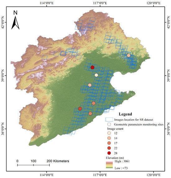
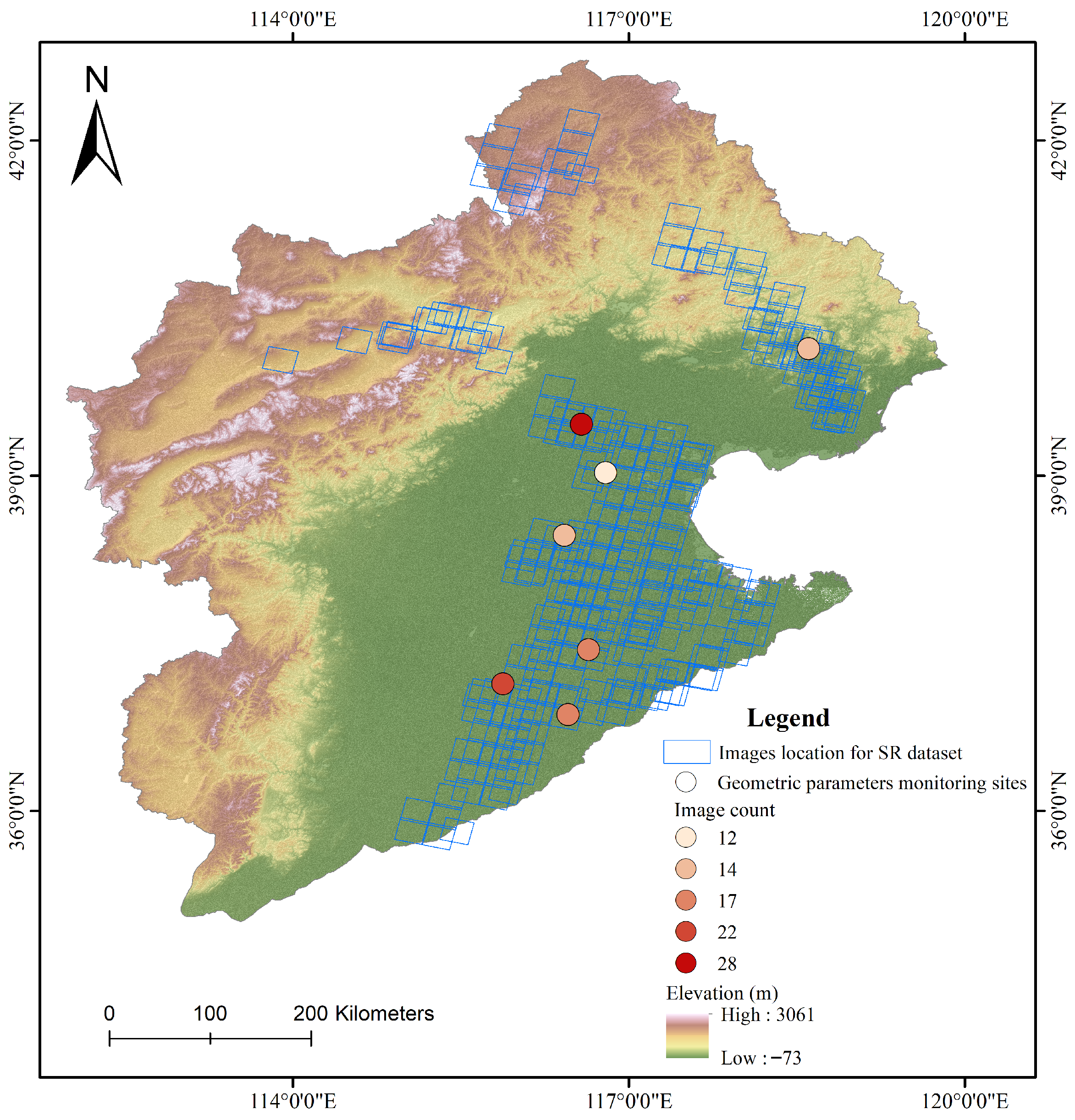
This study selected the Haihe River Basin as the research area (Figure 1). As a representative semi-humid to semi-arid basin in northern China, the Haihe River Basin is characterized by numerous small- and medium-sized rivers and complex channel morphologies. Strong anthropogenic disturbances have resulted in pronounced spatiotemporal heterogeneity and fragmentation across the basin.
Figure 1.
Study area of the Haihe River Basin. The blue rectangles indicate the geographical locations of commercial GF2 imagery used for training and validation of the SR model. The points represent the sites used for monitoring water geometric parameters, with the associated numbers indicating the count of GF2 imagery coverage at each site from 2020 to 2024.
In practical water body monitoring, the relatively narrow widths of small and medium-sized rivers lead to substantial mixed-pixel effects in conventional medium- to low-resolution remote sensing imagery, making it difficult to accurately delineate river boundaries and capture the spatial characteristics of fine tributaries. This limitation constrains the accuracy of high-precision dynamic monitoring based on remote sensing.
The basin encompasses diverse topographic units, including mountainous, hilly, and plain regions, providing strong spatial representativeness. Therefore, the Haihe River Basin serves as an ideal testbed for evaluating the effectiveness of SR methods in enhancing the monitoring accuracy of complex water bodies.
2.2. Remote Sensing Imagery
The remote sensing imagery utilized in this study comprises two components: one for constructing the SR dataset, and the other for temporal monitoring and change analysis of river geometric parameters.
To construct the HR database, a total of 331 GF2 multispectral images were obtained from the China Resources Satellite Application Center, covering the ice-free season from 28 March to 29 November 2024. Considering the focus on surface water monitoring, the downloaded imagery covers a 5 km buffer zone on both sides of the centerlines of first-order and second-order rivers in the Haihe River Basin. This region includes a wide variety of river morphologies, slopes, flow regimes, and environmental settings (Figure 1). The GF2 satellite, launched on 19 August 2014, carries an optical sensor suite comprising one panchromatic band and four multispectral bands (Blue, Green, Red, and Near-Infrared, BGRN). The spatial resolutions of the multispectral and panchromatic bands are 3.2 m and 0.8 m, respectively, with a 5-day revisit cycle and a 45 km dual-camera swath width.
During preprocessing, the GF2 multispectral imagery underwent radiometric calibration, atmospheric correction, and orthorectification. The panchromatic band, owing to its stable radiometric characteristics, did not require atmospheric correction. The preprocessed multispectral and panchromatic images were then pan-sharpened to generate a high-resolution reference image, which served as the geometric reference for subsequent registration of S2 imagery.
Compared with GF2’s four spectral bands, the S2 satellites provide 13 spectral bands spanning the visible to shortwave infrared range. Corresponding Sentinel-2A/B (S2A/B) images were downloaded from the Google Earth Engine (GEE) platform according to the spatial footprints of the GF2 images. To ensure spectral consistency, the B, G, R, and N bands were selected. Launched in 2015 and 2017, S2A and S2B offer a 10 m spatial resolution and a combined revisit time of approximately 5 days. To minimize temporal discrepancies caused by surface changes, S2 imagery was paired with GF2 scenes acquired within a ±5-day window (some images contained partial cloud cover).
In addition to the SR dataset, this study also processed time-series imagery from 2020 to 2024 for key monitoring sites within the Haihe River Basin, comprising 135 GF2 and 1529 S2 images. These datasets were used to monitor temporal variations in river geometric parameters. Unlike the SR dataset, the GF2 and S2 images here were not one-to-one paired but instead included all eligible scenes within the spatial and temporal windows of the study sites. All images were subjected to consistent preprocessing, including radiometric calibration, atmospheric correction, and orthorectification, following the same workflow as above, ensuring comparability and consistency across multi-temporal and multi-source datasets.
2.3. SR Dataset
2.3.1. Data Pairing
To train an SR deep learning model for water extraction, a training dataset composed of HR and LR image pairs must be constructed. Due to differences in pixel size, geometric projection, and spatial reference systems between GF2 and S2 imagery, achieving high-precision pairing required performing coordinate reprojection, resolution matching, and spatial registration steps.
To ensure spatial consistency between the S2 and GF2 imagery, the S2 data were first reprojected to match the UTM coordinate system of the GF2 imagery. After reprojection and grid alignment, the effective pixel size of S2 was adjusted from its nominal 10 m to approximately 8.9 m. This value was calculated based on the reprojected imagery and may be influenced by factors such as projection parameters and boundary cropping. The preprocessed GF2 imagery retained an effective spatial resolution of approximately 3.2 m (native resolution). To establish an integer scaling relationship between the two datasets for constructing the HR–LR pairs, cubic interpolation was applied to resample the S2 and GF2 imagery to 9 m and 3 m, respectively (ratio 3:1). The spatial overlap between the S2 and GF2 imagery was then extracted as the matching region. Finally, the 1 m fused GF2 panchromatic image was used as the geometric registration reference to ensure precise spatial alignment between the paired datasets. For HR imagery, a spatial resolution of 3 m enables the capture of relatively clear river boundaries and narrow water features, allowing for more accurate delineation of water extents. In contrast, LR imagery with a 9 m resolution is more prone to mixed pixel effects, which may lead to boundary blurring and reduced accuracy in representing small-scale or complex river structures.
To maintain spectral consistency across bands, this study constructed a four-band SR model specifically for the GF2 multispectral bands (B, G, R, N). The spectral ranges of each GF2 band are as follows: B (0.45–0.52 μm), G (0.52–0.59 μm), R (0.63–0.69 μm), and N (0.77–0.89 μm).
2.3.2. Dataset Parameters
SR models are typically trained in 8-bit unsigned integer (uint8) format, which exhibits minimal visual performance differences compared to higher-precision data while significantly improving computational efficiency and storage performance. Therefore, this study converted GF2 imagery to uint8 format to optimize computational resources.
Considering that training deep learning models directly on full-size images incurs substantial computational overhead and leads to class imbalance due to the low proportion of water pixels, this study adopted a patch-based training strategy. Specifically, GF2 imagery was cropped into 384 × 384 pixel tiles, while corresponding S2 imagery was cropped into 128 × 128 pixel tiles (the GF2 size is three times that of the S2). Tiles were cropped in a spatially continuous, spatially continuous and non-overlapping manner to ensure that no tile from a given GF2 image appears in both the training and validation sets, maintaining spatial independence between the subsets. After manual inspection, abnormal samples—including those affected by cloud and cloud-shadow contamination, snow and ice cover, striping noise, and missing imagery—were removed. Ultimately, a complete dataset consisting of 21,187 paired image patches was obtained.
The spatial extent of the dataset was defined as a 10 km corridor centered on the river centerline, with a 5 km buffer on each side. As this study targets full-scene water body SR, the model is required not only to learn the textural and spectral characteristics of water bodies, but also to capture the boundary features between water bodies and adjacent land-cover types, as well as the surrounding environmental context. Therefore, background samples without water bodies were retained in the dataset, which helps improve the model’s overall scene representation capability and generalization performance, while reducing the risk of overfitting to water-body regions.
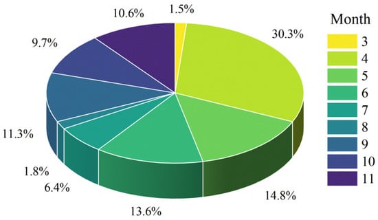
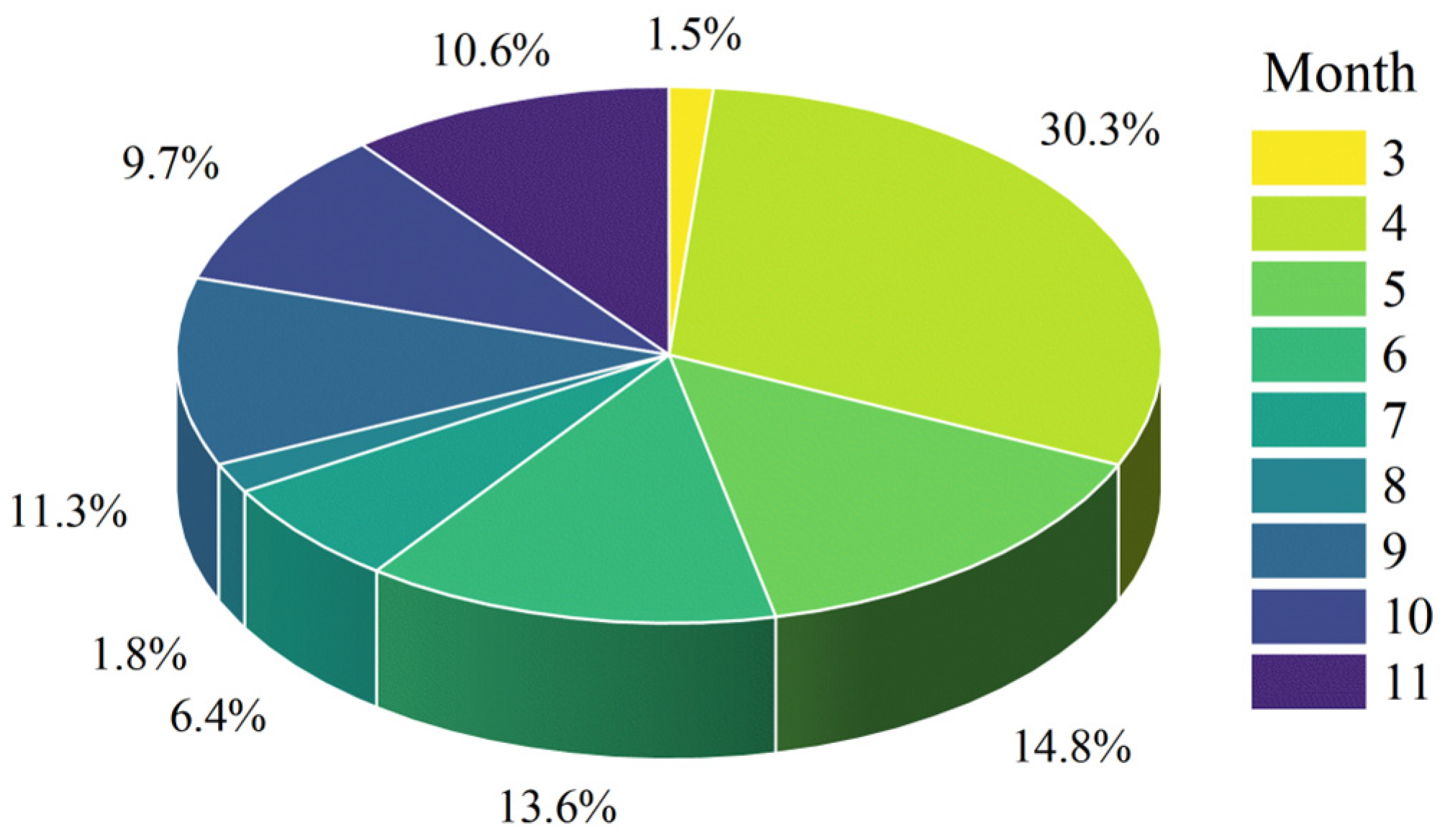
The temporal distribution of the dataset is shown in Figure 2. Except for March, when the number of samples is relatively low due to snow and ice coverage, August has the smallest proportion of samples at 1.8%, while April has the highest proportion at 30.3%. Overall, the temporal distribution of the samples is consistent with the characteristics of optical imagery, which is susceptible to extreme cloud cover and rainy weather conditions.
Figure 2.
The temporal distribution of the SR dataset.
For dataset partitioning, following standard machine learning practices, the dataset was divided into training (80%) and validation (20%) subsets. Specifically, 80% of the image pairs were used for model training, while 20% were reserved for validation and performance evaluation. To ensure temporal representativeness, the samples for each date were divided in an 80:20 ratio.
2.4. SR Deep Learning Model
This study aimed to enhance the accuracy and stability of water extraction by improving the spatial resolution of remote sensing imagery. This approach leveraged the rich spectral and spatial structural information contained within high-resolution imagery and offered high flexibility and scalability for subsequent multi-source remote sensing fusion, such as integration with radar imagery.
The Enhanced Super-Resolution Generative Adversarial Network (ESRGAN), an advanced SR model based on the GAN framework, effectively improved detail restoration capability and visual realism by introducing the Residual-in-Residual Dense Block (RRDB) structure [32]. It has demonstrated outstanding performance in SR tasks for natural images. However, remote sensing imagery differs substantially from natural images in spectral complexity and feature diversity. The direct application of ESRGAN often results in spectral distortion and blurred feature boundaries. Therefore, this study developed an improved model—the AESRGAN—by building upon the ESRGAN architecture and incorporating spectral consistency constraints and feature preservation mechanisms specifically designed for remote sensing imagery. The following sections describe the deep learning network architecture and the design of the AESRGAN model.
2.4.1. Generator Architecture
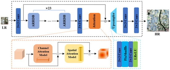
The overall architecture of the generator network consists of a shallow feature extraction module, a deep feature learning module, an attention mechanism module, and an up-sampling reconstruction module (Figure 3).
Figure 3.
Network architecture of the generator in the AESRGAN model.
The initial convolutional layer of the generator performs shallow feature extraction on LR input images:
where ILR is the low-resolution input image with a size of 128 × 128 × 3, and F0 is the extracted shallow feature map with a size of 128 × 128 × 64.
Subsequently, the shallow feature F0 is fed into a deep feature extraction module composed of n cascaded Attention Residual-in-Residual Dense Blocks (ARRDB) to model the complex spatial and spectral features of the image. To achieve global residual learning, long-jump residual connections are established between the first convolutional layer and the last ARRDB to facilitate stable propagation of deep features:
where ARRDBN is the Nth ARRDB (23 ARRDBs were used in this study). The size of the deep feature Fdeep remains 128 × 128 × 64 after the deep feature extraction module. The number of 23 ARRDB modules is inherited from the original ESRGAN, which has been empirically validated to balance network capacity, training stability, and computational cost. As our ARRDB only introduces an attention mechanism without altering the network depth, we retain this configuration to ensure fair comparison and stable training.
Following deep feature extraction, the model incorporates a global attention module to further refine features. This module combines channel attention and spatial attention mechanisms to capture long-range dependencies across a larger receptive field, thereby enhancing the model’s perception of details such as textures and edges. Next, the feature maps undergo resolution enhancement through an upsampling and reconstruction module. This module consists of a sub-pixel convolution layer (PixelShuffle) and two standard convolution layers, enabling efficient spatial reconstruction:
where PixelShuffle denotes the sub-pixel convolution layer that realizes 3× upsampling. The final reconstructed SR image Fsr has a size of 384 × 384 × 3.
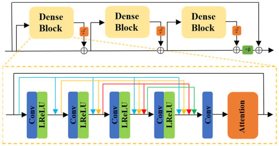
The ARRDB module (Figure 4) is designed as an improved structure that integrates an attention mechanism into the Residual-in-Residual Dense Block (RRDB) used in ESRGAN. RRDB consists of multiple cascaded Residual Dense Blocks (RDBs), each containing five convolutional layers with ReLU activation functions. Dense connections enable layer-by-layer feature accumulation and reuse, thereby extracting rich local features. The residual scaling factor in RRDB helps mitigate gradient explosion and stabilize the training process.
Figure 4.
Details of the Attention Residual-in-Residual Dense Block (ARRDB).
This study introduces the Convolutional Block Attention Module (CBAM) attention mechanism after the residual in RRDB to enhance the generator’s perception of key spectral and spatial features in remote sensing imagery. CBAM comprises the Channel Attention Module (CAM) and Spatial Attention Module (SAM), which sequentially operate on the channel and spatial dimensions of feature maps [39]. Specifically, CAM generates channel weight vectors through global average pooling and max pooling operations to highlight crucial spectral information. SAM generates spatial weight maps via convolutional operations to emphasize feature boundaries and texture details. This hierarchical attention enhancement mechanism enhances the model’s ability to capture complex feature characteristics in multispectral remote sensing imagery.
The CAM adaptively assigns higher weights to important spectral channels by capturing interdependencies among channels:
where F is the input feature map; AvgPool and MaxPool are global average pooling and max pooling operations, respectively; MLP is a multi-layer perceptron; and σ is the sigmoid activation function.
The SAM models positional dependencies in the spatial dimension of feature maps, enhancing the model’s response to key feature regions:
where f7×7 is a 7 × 7 convolution operation; [·;·] is concatenation along the channel dimension; AvgPool and MaxPool are average and max pooling operations along the channel dimension, respectively; σ is the Sigmoid activation function.
2.4.2. Discriminator Architecture
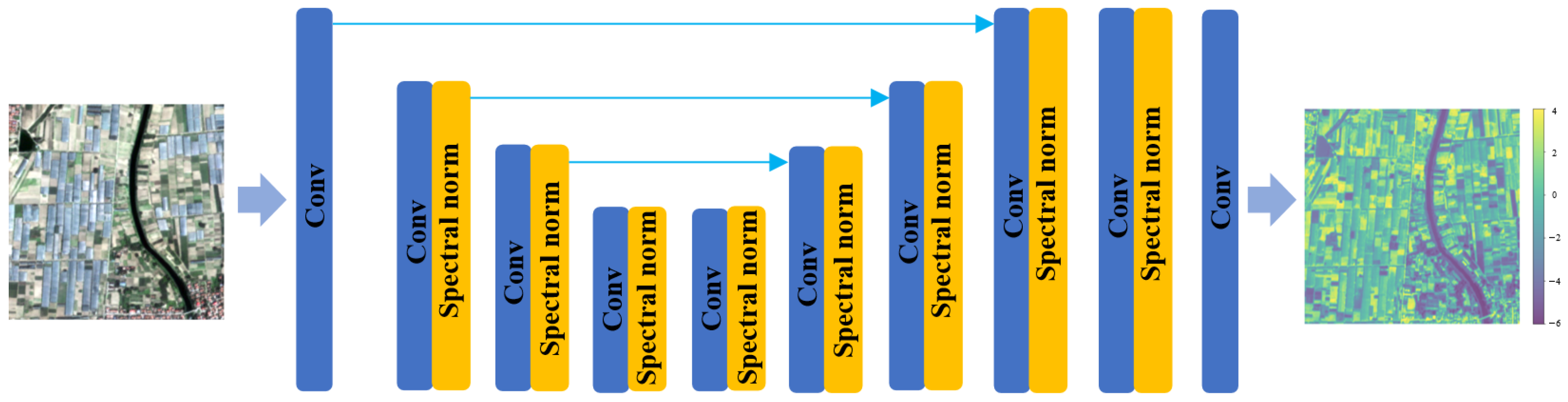
The discriminator is modified from a VGG backbone to a U-Net architecture with skip connections (Figure 5) [40]. The U-Net outputs authenticity scores for each pixel, enabling detailed per-pixel feedback to the generator. Concurrently, spectral normalization regularization is employed to stabilize training dynamics and mitigate sharp artifacts introduced by GAN training. This adaptation enables the discriminator to capture both local and global features effectively.
Figure 5.
U-Net architecture with spectral normalization.
2.5. Loss Function
The loss function plays a crucial role in deep learning models by measuring the discrepancy between predicted and true results. Its design directly determines the optimization direction and reconstruction performance of the model. Considering the characteristics of remote sensing imagery, this study introduces spectral consistency and structural preservation constraints into the original ESRGAN loss framework, enhancing the model’s ability to preserve feature boundaries and spectral fidelity.
where LG is the total loss of the generator, Lpix is the pixel loss, Lpercep is the perceptual loss, Lgan is the generator adversarial loss, Lspectral is the spectral loss, and Lssim is the structural similarity loss. λpix, λpercep, λgan, λspectral, and λssim serve as weighting coefficients. In this study, λpix = 1, λpercep = 1, λgan = 0.1, λspectral = 0.2, and λssim = 0.5.
The discriminator loss function is defined as:
where LD is the total loss of the discriminator, Lreal is the real data loss, and Lfake is the generated data loss.
2.6. Model Training Settings
The model was trained using the PyTorch 2.3.0 (CUDA 12.1) on a single NVIDIA GeForce RTX 3090 (24 GB) graphics card produced by NVIDIA (Santa Clara, CA, USA). The key training parameters are summarized as follows:
Optimizer and learning rate: Both the generator and discriminator were optimized using the Adam optimizer with an initial learning rate of 1 × 10⁻⁴, no weight decay, and momentum parameters β1 = 0.9 and β2 = 0.99. A MultiStepLR scheduler was employed, reducing the learning rate by 50% at 400,000 iterations.
Batch size and iterations: The batch size per GPU was 4, with 4 worker threads for data loading. The total number of training iterations was 400,000, and no warm-up iterations were applied.
Generator initialization: The generator was initialized with pre-trained weights from RealESRNet_x4plus provided by Tencent ARC Lab (Shenzhen, China), and parameters were strictly loaded to ensure stable initialization.
Data augmentation: During training, input samples were augmented using horizontal flips, while no augmentation was applied during validation.
2.7. Water and Geometric Parameters Extraction Methods
2.7.1. Water Extraction Methods
Since GF2 and ASR imagery only contain four spectral bands—B, G, R, and N—water extraction methods that are partially dependent on mid-infrared or shortwave infrared bands (such as Modified Normalized Difference Water Index MNDWI, Automatic Water Extraction Index AWEI, and methods based on the HSV color space) are inapplicable.
For the three types of remote sensing data involved in this study (S2, GF2, and ASR imagery), eight water extraction methods were compared to achieve optimal water identification in the study area. Normalized Difference Water Index (NDWI) was selected as a representative water index due to its widespread use and robust performance in water body extraction tasks [41]. Specifically, two threshold-based methods were employed: NDWI combined with Otsu’s thresholding (NDWI + Otsu) and NDWI combined with K-means clustering (NDWI+ KM) [42,43,44,45]. In addition, four machine learning algorithms—Random Forest (RF), Support Vector Machine (SVM), Decision Tree (DT), and K-Nearest Neighbors (KNN)—were implemented, along with two deep learning models, U-Net++ and DeepLabv3+ (https://blog.csdn.net/m0_37799466/article/details/103469384 (accessed on 10 March 2026)) [46,47,48,49,50,51]. In feature construction for machine learning models, NDWI and NDVI indices were incorporated alongside the four bands of the original imagery to enhance the model’s discrimination capability at water-land boundaries.
The construction of training samples is a critical step in training water extraction models. To ensure representativeness and diversity, 129 images from S2, GF2, and ASR were selected, covering different river reaches and temporal phases within the Haihe River Basin. Pixel-level samples were annotated using manual visual interpretation. Each pixel in the images was classified as water (1) or non-water (0). Among these, 109 images were used for model training, while 20 images were reserved for accuracy validation and confusion matrix analysis. To balance storage efficiency and computational performance, the sample data was stored in uint8 format.
Of the 109 training samples used for water extraction, 17 exhibited spatial overlap with samples from the SR dataset. In contrast, none of the 20 validation samples overlapped spatially with any samples used in the SR training or validation sets. This ensures that the evaluation of water extraction performance is conducted on spatially independent data, thereby avoiding potential bias.
2.7.2. River Length and Width Extraction Methods
Based on the extracted water bodies, the river centerline is extracted to determine the river length. The main steps include: (1) Riverline extraction: Obtain the polygonal lines along both banks of the water; (2) Bankline pairing: Through buffer analysis and topological connectivity, selecting boundaries that are relatively similar in width, generally aligned in direction, and topologically adjacent to each other as a pair of banklines; (3) Corresponding point matching: At each vertex of a shoreline, locate the corresponding point on the opposite bank using the nearest neighbor method; (4) Centerline generation: Calculate the geometric midpoints of corresponding points and connect multiple midpoints along the river direction to form an initial centerline; (5) Geometric optimization: Smoothing and performing topological repair operations on the initial centerline to obtain the river centerline.
The river centerline length represents the river length. River width is calculated as the length of line segments perpendicular to the river centerline and intersecting both river banks.
2.8. Evaluation Metrics
2.8.1. Metrics for Super-Resolution Reconstruction
The SR reconstruction results of remote sensing imagery should be visually realistic and exhibit high fidelity in spectral consistency. Therefore, we employ three metrics—Peak Signal-to-Noise Ratio (PSNR), Structural Similarity Index Measure (SSIM), and spectral loss—to assess model performance.
PSNR evaluates image distortion, where higher values indicate lower image distortion:
where C, H, and W denote the channel, height, and width of the SR image.
SSIM measures the structural similarity between two images, considering luminance, contrast, and structure. Its value ranges from 0 to 1, with values closer to 1 indicating higher similarity:
where μ and σ denote the mean and variance of the image, respectively. The constants C1 = (k1L)2 and C2 = (k2L)2 represent the dynamic range of pixel values, where L denotes the dynamic range of pixel values. Typically, k1 = 0.01 and k2 = 0.03.
Spectral Loss quantifies the deviation in spectral information between the super-resolved image and the reference HR image. A smaller spectral loss indicates better spectral consistency:
where N, H, and W denote the number of image channels, height, and width, respectively. and represent the spectral reflectance values of the SR image and the reference HR image, respectively. ϵ is a small constant to avoid division by zero.
2.8.2. Metrics for Water and Geometric Parameter Extraction
The accuracy of water extraction was evaluated using overall accuracy (OA) and the Kappa coefficient from the confusion matrix. OA is the proportion of correctly classified samples relative to the total sample count, while the Kappa coefficient accounts for random agreement. Higher OA and Kappa values indicate superior reliability and stability of water classification:
where CM [i, i] is the number of correctly classified samples in class i within the confusion matrix, and n represents the total number of samples and the number of classes.
where OA is the overall accuracy, and OAchance represents the expected accuracy of random classification.
For geometric parameters, relative error (RE) is used to evaluate water extraction accuracy, while mean absolute error (MAE) and root mean square error (RMSE) are used to assess the accuracy of time-series river width extraction:
where n is the total number of samples, VM is the extracted value, and VT is the true value.
3. Results
3.1. Performance of SR Models
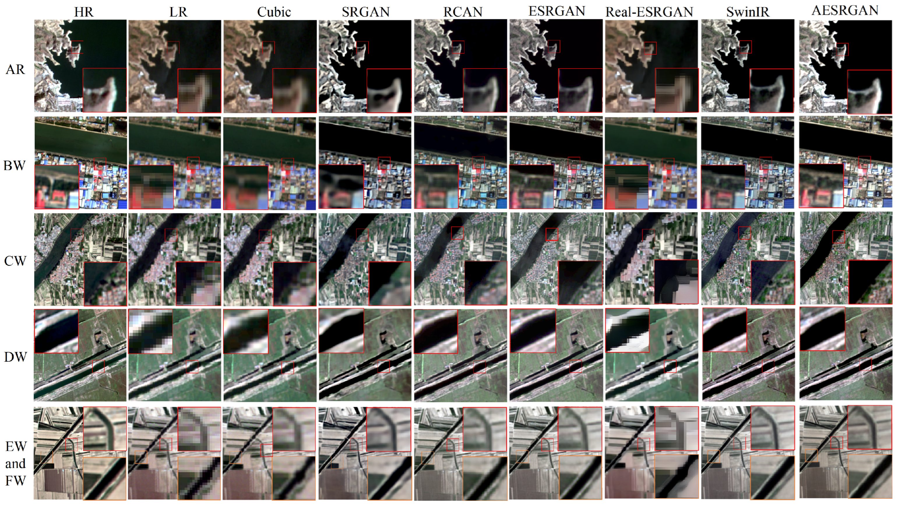
To evaluate the applicability and performance of the AESRGAN model on water of varying scales, this study selected satellite imagery covering multi-scale river widths, including reservoirs (AR), 320 m-wide rivers (BW), 154 m-wide rivers (RW), 62 m-wide rivers (DW), 31 m-wide rivers (EW), and 16 m-wide rivers (FW).
Seven SR methods were applied to these datasets, including cubic interpolation, SRGAN, Residual Channel Attention Network (RCAN), ESRGAN, Real-ESRGAN, Swin Transformer for Image Restoration (SwinIR), and the AESRGAN model. Among them, RCAN is a typical CNN-based model with an effective channel attention mechanism for accurate image reconstruction; SwinIR is a representative Transformer-based model widely used in remote sensing image processing; and Real-ESRGAN is an enhanced version of ESRGAN designed for real-world image degradation.
As shown in Figure 6, the comparison results indicate that the AESRGAN model demonstrates superior performance in detail restoration, structural preservation, and visual realism. Specifically, images generated by the AESRGAN model exhibit clearer water–land boundaries, smoother river textures, and more natural detail transitions. Particularly in small-scale river scenarios (e.g., FW), AESRGAN effectively suppresses blurred edges and enhances texture continuity, enabling more accurate reconstruction of narrow river reaches and tributaries. These results highlight its advantages over the other methods.
Figure 6.
Comparison of image reconstruction results among different SR methods. In “EW and FW”, the orange box represents EW and the red box represents FW.
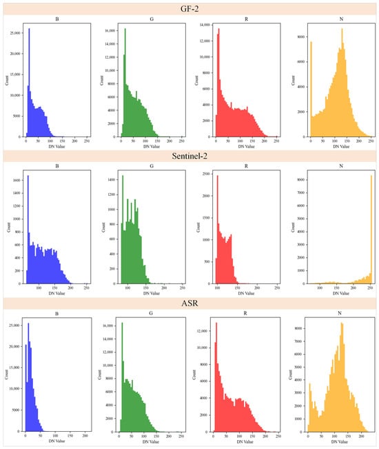
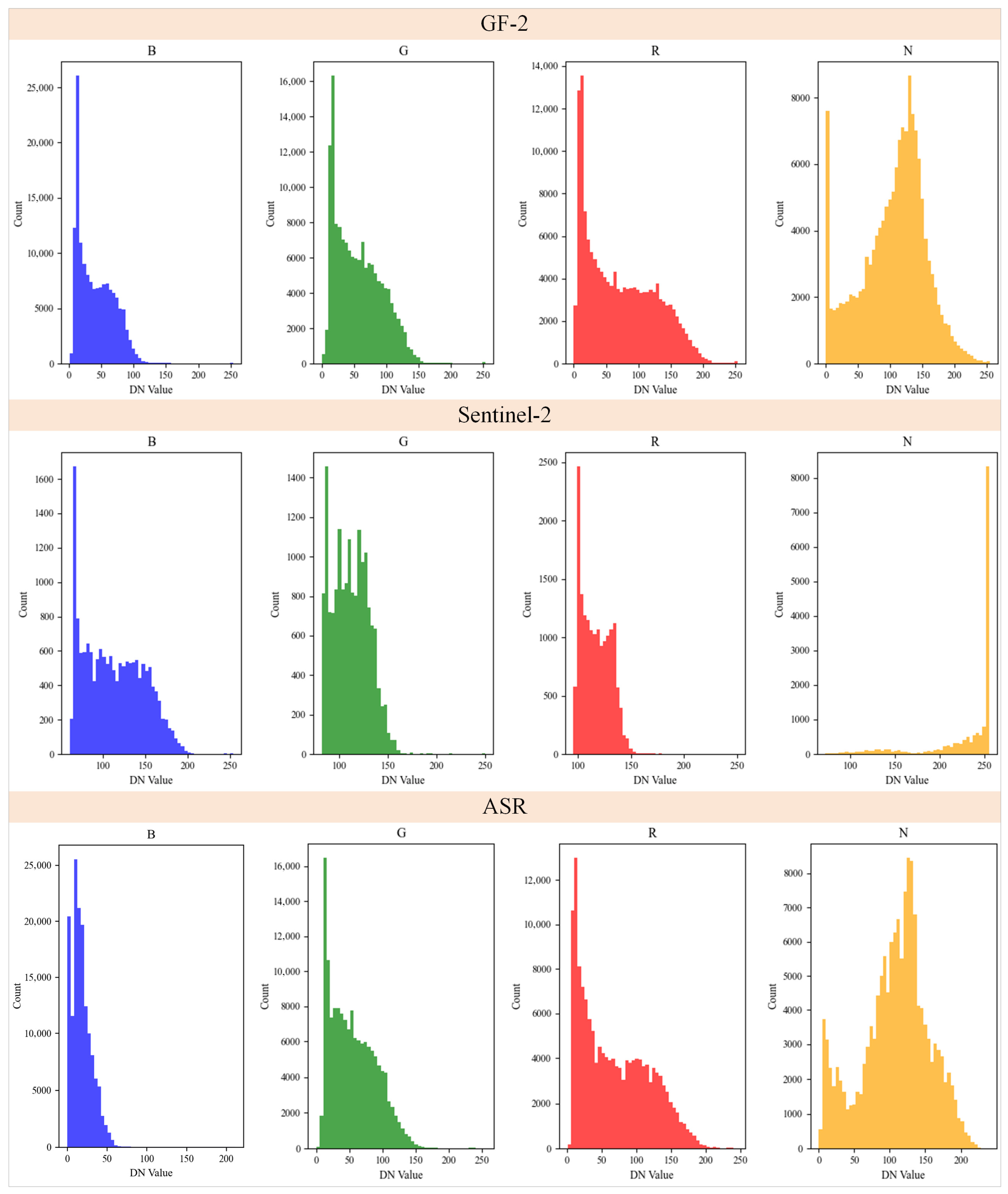
Furthermore, spectral features play a crucial role in water extraction. To assess the impact of AESRGAN on spectral fidelity, the spectral distribution of four bands (B, G, R, and N) was analyzed (Figure 7). The results show that the AESRGAN model can effectively reconstruct the spectral distribution of S2 imagery, rendering the spectral characteristics of ASR imagery highly consistent with GF2 imagery, thereby validating the spectral fidelity of AESRGAN.
Figure 7.
Spectral distribution statistics of GF2, S2, and ASR imagery.
3.2. Water Extraction Results
To accurately assess the impact of the AESRGAN model on water monitoring accuracy, S2, GF2, and ASR imagery from major river reaches were selected. Eight water extraction methods—NDWI + Otsu, NDWI + KM, DT, RF, SVM, KNN, U-Net++, and DeepLabv3+—were applied to these datasets, and the optimal extraction method for each imagery type was determined.
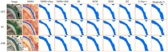
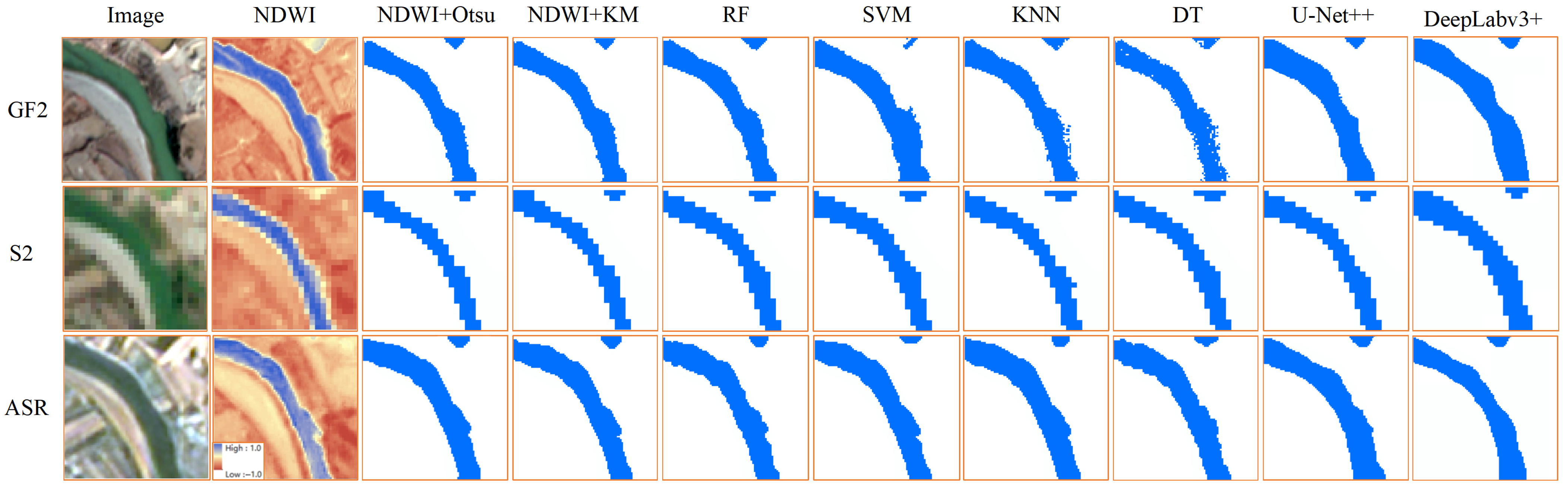
Figure 8 compares the extraction results of different methods on a typical river reach. The results show that the GF2 raw imagery exhibits clear textures, with extracted water boundaries appearing continuous and closely matching the actual water morphology. In contrast, the S2 imagery, due to its 10 m spatial resolution, shows pronounced pixelation effects, resulting in coarse water boundaries with evident jagged edges that fail to accurately represent the true river morphology. The ASR imagery enhances spatial detail, improves water boundary continuity and regional coherence, and yields extraction results that visually approach those of the GF2 imagery.
Figure 8.
Comparison of water extraction results using eight methods on GF2, S2, and ASR imagery.
Confusion matrices were calculated for the extraction results, and the performance of each method was evaluated using the average OA value and the average Kappa coefficient for each river reach (Table 1). Detailed results across river segments are provided in Appendix B.
Table 1.
Accuracy assessment of water monitoring based on the confusion matrix.
For S2 imagery, the U-Net++ method demonstrated the highest overall accuracy (OA) at 0.94. The NDWI + KM and NDWI + Otsu methods followed with an OA of 0.93 each. The DeepLabv3+, DT and RF methods achieved an OA of 0.92. The SVM method exhibited the lowest overall accuracy at 0.89. For GF2 imagery, NDWI + Otsu performed best with an OA of 0.98. U-Net++, DeepLabv3+, SVM, RF, and KNN followed, all achieving an OA of 0.97, DT obtained 0.96; while NDWI + KM had the lowest OA at only 0.88. For ASR imagery, U-Net++ achieved the highest accuracy with an OA of 0.97; DeepLabv3+, KNN and NDWI + Otsu followed with an OA of 0.96; SVM reached 0.95; RF attained 0.94; NDWI + KM achieved 0.93; and DT had the lowest accuracy at 0.92. Overall, the AESRGAN model improves water extraction accuracy for S2 imagery, bringing its performance across multiple methods closer to that of GF2 imagery.
3.3. Extraction of Water Geometric Parameters
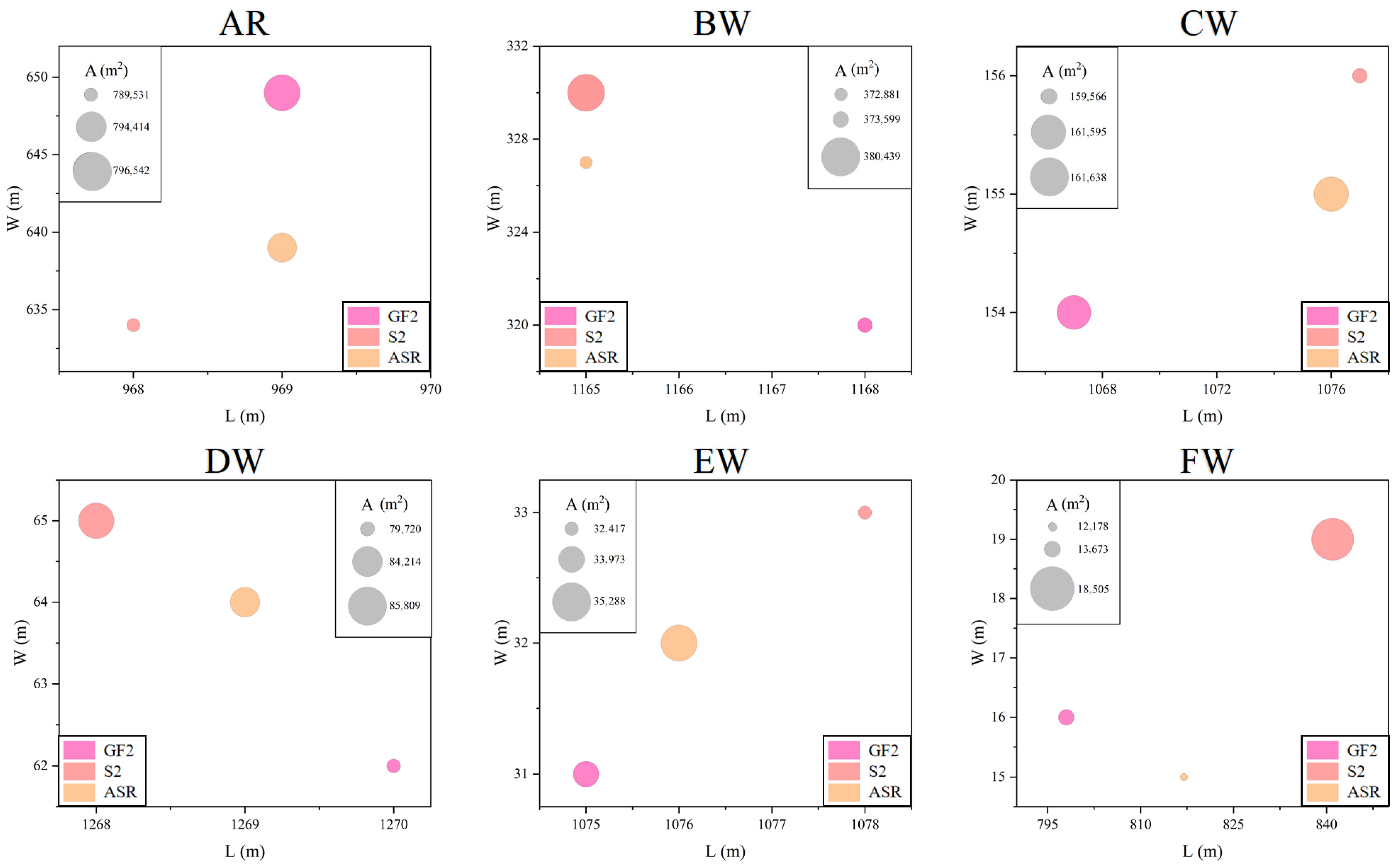
Optimal water extraction methods for different imagery types were employed to derive geometric parameters (L, W, A) for river reaches at multiple scales (Figure 9). The results indicate that both the spatial resolution of the imagery and the SR processing influence the accuracy of water geometric parameter estimation, with varying responses observed across different river scales.
Figure 9.
Extraction results of river geometric parameters at multiple spatial scales. The horizontal axis represents the L extracted for the river section, and the vertical axis represents the W extracted. The circles in the A (m2) legend represent the size of the extracted area A. The magenta color represents the GF2 image, the pink color represents the S2 image, and the orange color represents the ASR image.
GF2 imagery demonstrates advantages in quantifying geometric parameters across all water scales. For large-scale water, its L, W, and A measurements exhibit high consistency; for small-scale water, its quantification errors remain relatively small, indicating that GF2 imagery can accurately capture river boundary information. In contrast, S2 imagery generally exhibits larger errors in geometric parameter extraction, particularly for small-scale water (e.g., EW, FW). This is mainly due to the 10 m spatial resolution, which limits its ability to effectively capture narrow water edges. The AESRGAN model improves the accuracy of geometric parameter extraction for all river reaches. For large-scale water, the geometric parameters derived from ASR imagery closely approximate those from GF2 imagery, demonstrating the effectiveness of the AESRGAN model in restoring spatial details. For small-scale water, although the improvements are limited, they still show enhancement compared with S2 imagery. Overall, high-resolution imagery remains the preferred data source for extracting water geometric parameters, while the AESRGAN model can effectively improve the accuracy of S2 imagery.
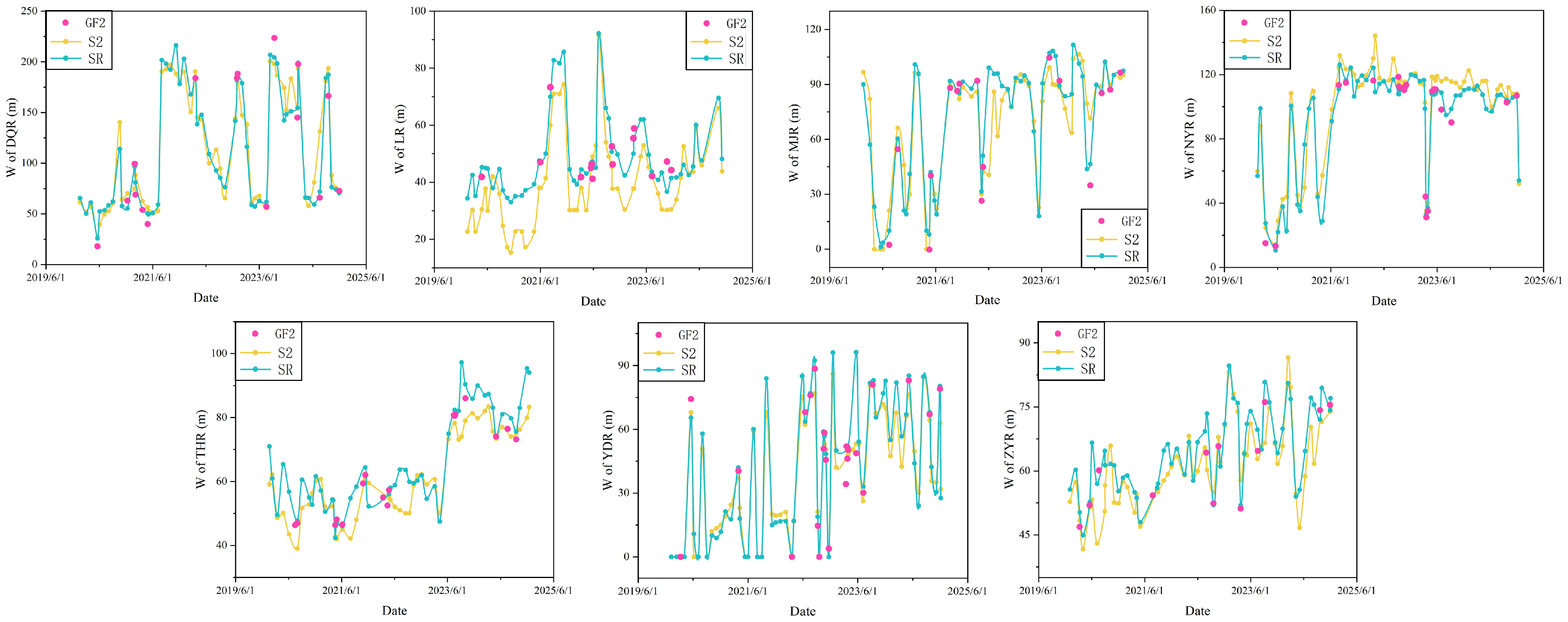
Time series river width data from 2020 to 2024 were extracted at major monitoring points (Figure 10). The river width derived from ASR imagery shows high consistency with GF2 imagery, exhibiting stable time-series patterns and good fitting accuracy, with MAE and RMSE of 3.66 and 5.53, respectively. In contrast, due to spatial resolution limitations, S2 imagery shows larger absolute deviations and distorted temporal patterns, with MAE and RMSE of 6.99 and 9.48, respectively.
Figure 10.
Time series of river width at major monitoring points from 2020 to 2024. The magenta dots represent river widths derived from GF2 imagery, while the yellow and green lines denote those derived from S2 and ASR imagery, respectively. For dates with available GF2 observations, all three data sources (GF2, S2, and ASR) are retained. For months without GF2 imagery, one representative river width is selected from each of S2 and ASR to ensure temporal continuity.
The above results indicate that, in months where GF2 imagery is unavailable, river widths derived from ASR can provide reliable estimates that closely approximate those from GF2. In contrast, widths extracted from S2, while exhibiting relatively lower precision, still effectively capture the overall temporal trends and seasonal patterns of river width variations. In the multi-source data fusion for time-series construction, although S2 and ASR introduce certain uncertainties, their impact on long-term trend analysis remains limited. Therefore, in long-term multi-source remote sensing data fusion, the SR method can effectively mitigate uncertainties arising from the absence of high-resolution data, thereby providing more continuous and higher-precision river width time-series support.
4. Discussion
4.1. SR Remote Sensing Dataset
The quality of training datasets typically exerts a decisive influence on the accuracy and generalization performance of SR models [52]. In the field of remote sensing, several publicly available datasets derived from aerial and satellite imagery have been used for SR tasks, such as the UC Merced dataset [53], the ISPRS Vaihingen and Potsdam datasets [54,55], AID [56], DOTA [57,58], WHU-RS19 [59,60], RSSCN7 [61], and NWPU-RESISC45 [62]. However, these datasets were originally developed for tasks like scene classification and object detection, resulting in inconsistent image sources and spatial resolutions across datasets. Consequently, the direct use of these publicly available datasets does not necessarily yield optimal training performance for SR models.
Some studies have purposefully constructed datasets between relatively high-resolution and relatively low-resolution satellites based on specific research objectives. For instance, ref. [16] developed an SR model for Landsat-8 (15 m, 30 m) and S2 (10 m, 20 m) to observe the Normalized Difference Vegetation Index (NDVI). Reference [35] created an SR dataset combining S2 (10 m) and commercial WorldView (2 m) imagery for water segmentation. However, due to the high cost of acquiring genuine HR imagery and the difficulty in registering corresponding LR data, publicly available datasets remain scarce.
This study constructs a GF2–S2 remote sensing SR dataset based on high-resolution GF2 imagery and medium-resolution S2 imagery. Through radiometric calibration, geometric correction, reprojection, resolution resampling, and sub-pixel spatial registration, paired HR-LR training samples were established. This dataset exhibits high consistency in both spatial and spectral dimensions, providing authentic, reliable and physically meaningful data support for SR research in remote sensing imagery.
This study adopted bicubic interpolation as the primary resampling kernel, primarily due to its widespread use in remote sensing super-resolution research and its favorable engineering properties. Specifically, the bicubic kernel offers high computational efficiency, minimal ringing artifacts, and good preservation of spectral continuity [63], which is beneficial for maintaining spectral fidelity in downstream water body extraction tasks [64]. However, owing to its inherent low-pass filtering characteristics, bicubic interpolation attenuates mid- to high-frequency components to some extent, potentially leading to partial loss of high-frequency details and slight smoothing or blurring at water boundaries—particularly in narrow channels, vegetated areas, or complex land–water transition zones. In contrast, Lanczos interpolation better preserves high-frequency edge information and improves boundary sharpness and positional accuracy but is more prone to introducing ringing artifacts and spectral leakage; Gaussian kernels tend to over-smooth and lose critical high-frequency details, which is disadvantageous for precise boundary delineation in complex water bodies. Therefore, bicubic provides a reasonable trade-off between spectral fidelity and boundary precision.
It should be noted that, although the choice of resampling kernel affects frequency response and boundary accuracy to some degree, all training and testing samples in this study were processed with the same bicubic kernel. Consequently, this influence remains consistent across all methods and does not introduce systematic bias favoring any particular model. Furthermore, the primary focus of this work is to evaluate the ability of super-resolution methods to recover spatial details under a unified degradation model assumption. Thus, the adopted bicubic resampling strategy provides a stable, controllable, and fair experimental foundation for relative performance comparison.
Furthermore, considering the potential spatial correlation introduced by random date-based data partitioning, a supplementary experiment based on a scene-level splitting strategy was conducted. In this setting, all tiles originating from the same GF2 scene were exclusively allocated to either the training or validation set to ensure strict spatial independence. Detailed experimental configurations, quantitative results, and comparative analyses are presented in Appendix A. The consistency of model performance under this more rigorous evaluation protocol further validates the generalization capability and robustness of the proposed approach.
4.2. Accuracy of the SR Model
To evaluate the performance of different SR models in remote sensing image reconstruction tasks, this study calculated the PSNR, SSIM, and spectral loss metrics for the cubic interpolation, SRGAN, RCAN, ESRGAN, Real-ESRGAN, SwinIR, and AESRGAN models (Table 2). These three metrics reflect the comprehensive performance of the models from three perspectives: geometric detail restoration, structural preservation, and spectral consistency.
Table 2.
PSNR, SSIM, and spectral loss for different SR methods.
The results demonstrate that the AESRGAN model achieved optimal performance across all three metrics. Specifically, the PSNR reached 33.83, indicating a clear advantage in pixel-level reconstruction accuracy. The SSIM value of 0.882 further demonstrates the model’s enhanced capability to preserve spatial structures and textural relationships of surface features. Meanwhile, the spectral loss decreased to 0.008, highlighting the superior ability of AESRGAN to maintain spectral consistency. These improvements can be attributed to the integration of attention mechanisms and the proposed spectral–structural loss design. The attention modules enhance the representation of complex spatial features, particularly at water–land boundaries, leading to improved structural fidelity. At the same time, the spectral constraint effectively suppresses spectral distortion during the reconstruction process, which is essential for maintaining the physical meaning of multispectral data. This improvement in spectral fidelity is particularly critical for remote sensing applications, as it reduces spectral aliasing effects caused by reconstruction artifacts and improves the stability and reliability of downstream tasks such as water body extraction and classification.
To further evaluate the effectiveness of the proposed attention mechanism and loss function, two model variants—AESRGAN-ARRDB and AESRGAN-LF—were constructed, and ablation experiments were conducted. The results are summarized in Table 3. The experimental results show that, compared with the baseline model, the AESRGAN-ARRDB variant achieves improvements of 0.78 dB, 0.004, and 0.001 in terms of PSNR, SSIM, and spectral loss, respectively. These results indicate that the ARRDB module incorporating the CBAM attention mechanism effectively enhances the model’s ability to capture salient structural features, such as image textures and land-cover boundaries, thereby improving the spatial reconstruction accuracy and structural fidelity of the generated images. In addition, the AESRGAN-LF variant improves PSNR, SSIM, and Spectral Loss by 0.63, 0.03, and 0.02, respectively. This demonstrates that the designed loss function provides more effective optimization constraints during model training, enabling the reconstructed images to achieve improved spectral consistency and visual quality.
Table 3.
Ablation Experiment Results.
Overall, the ablation results confirm that the proposed attention-enhanced architecture and loss function design contribute to improving the performance of remote sensing image super-resolution reconstruction.
Although the proposed model is validated on the self-constructed GF2–S2 dataset, its design is not limited to a specific dataset. The AESRGAN framework is fundamentally data-driven and incorporates attention mechanisms together with spectral–structural constraints, enabling it to generalize to remote sensing imagery with similar spectral configurations.
4.3. Extraction of Water and Geometric Parameters
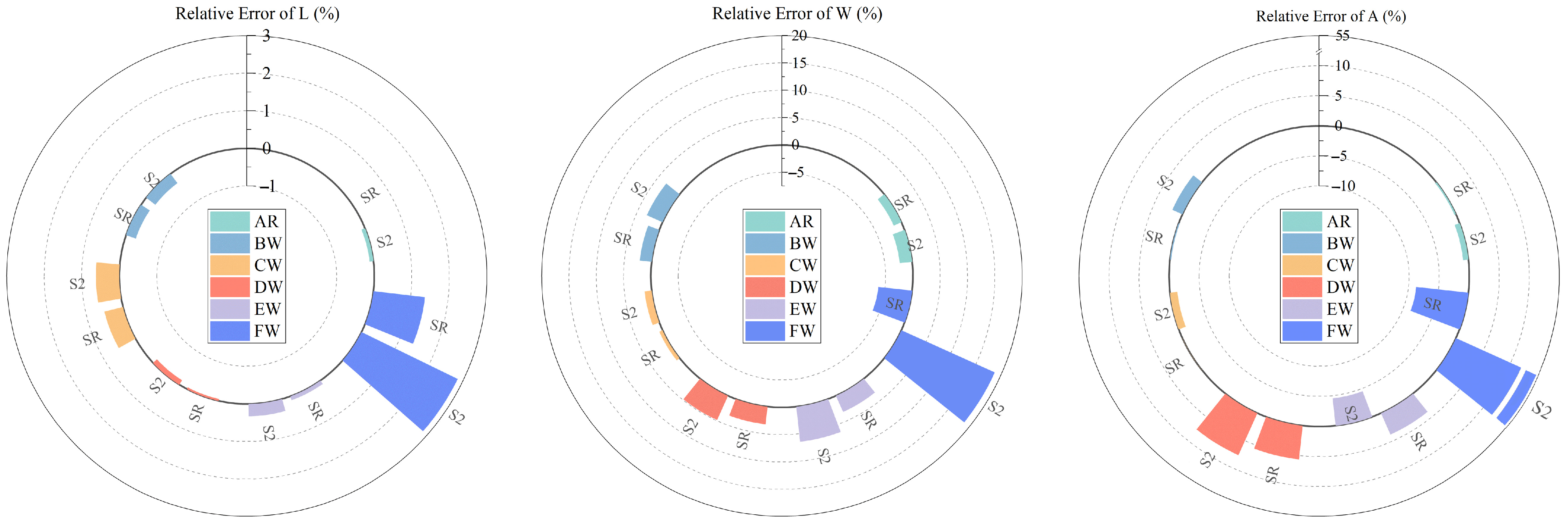
When extracting water geometric parameters through multi-resolution remote sensing image fusion, inconsistencies between datasets are often observed. Some studies employ linear regression or proportional coefficients to improve the consistency and accuracy of water geometric parameters [13]. In this study, water geometric parameters derived from GF2 imagery were used as a high-resolution reference (rather than absolute ground truth) due to its superior spatial resolution. To ensure a reliable evaluation, relative errors (RE) of river length (L), width (W), and area (A) were calculated for representative river reaches (AR, BW, CW, DW, EW, FW) (Figure 11), thereby quantitatively assessing the impact of AESRGAN on data discrepancies. It should be noted that although GF2 imagery provides finer spatial details, uncertainties may still exist due to factors such as water boundary delineation, mixed pixels, and potential interpretation errors. Therefore, the reported evaluation results should be interpreted as relative comparisons rather than absolute accuracy assessments.
Figure 11.
Accuracy of water geometric parameter monitoring.
For L, the RE values of both S2 and ASR imagery were relatively low, with absolute RE values below 1% in most river reaches. In FW, the ASR imagery RE (1.38%) was lower than that of S2 imagery (2.85%). Overall, ASR imagery demonstrated slightly higher accuracy than S2 imagery. This stems from river length estimation being primarily influenced by spatial structural continuity, with minimal influence from mixed-pixel effects. For W, ASR imagery exhibited higher accuracy across all river reaches, with a particularly significant gap in the FW segment where the absolute RE value decreased from 18.75% (S2 imagery) to 6.25% (ASR imagery). RE exhibited a trend varying with river reach width (W): smaller widths correspond to larger RE values. For A, most scales showed S2 image RE values ranging from −0.88% to 7.64%. However, in FW, S2 imagery RE reached 53.59%, indicating significant bias. In contrast, ASR imagery RE was −8.74%, demonstrating markedly improved overall accuracy. Compared to S2 imagery, ASR imagery achieved accuracy improvements of 0.34%, 3.28%, and 8.51%, for river L, W, and A, respectively. All error values exhibited random characteristics within the positive and negative ranges, indicating the absence of systematic bias.
The improvement in water extraction and geometric parameter estimation accuracy can be mainly attributed to the enhanced spatial resolution and clearer boundary representation, which effectively reduce mixed-pixel effects and improve the separability between water and land. The observed trend that smaller river widths correspond to larger relative errors further highlights the limitation of medium-resolution imagery in capturing small and narrow river features. Super-resolution reconstruction alleviates this issue by refining fine-scale spatial details, thereby improving the monitoring capability for narrow rivers.
Overall, the results demonstrate that the proposed AESRGAN model not only improves image quality but also enhances the reliability of geometry-based hydrological parameter estimation, particularly in scenarios where boundary precision is critical.
5. Conclusions
This study addresses the core contradiction in current remote sensing water monitoring: insufficient resolution of publicly available data versus limited coverage of high-resolution data. It constructs a GF2–S2 paired super-resolution dataset and proposes an AESRGAN model integrating attention mechanisms and multi-constraint loss functions. A technical methodology system of “low-resolution imagery→super-resolution reconstruction→high-precision water information extraction” is established, providing an innovative solution for low-cost, large-scale, and refined surface water monitoring. The core innovative value of this research lies in alleviating the inherent trade-off between spatial resolution and coverage in traditional remote sensing monitoring, providing a novel low-cost, high-precision data acquisition path for hydrological and water resource remote sensing monitoring. In addition, the proposed framework offers methodological insights for related fields, including multi-source remote sensing data fusion and fine-grained land-cover classification.
In terms of application expansion, this method can be directly used for river runoff inversion. Based on high-precision geometric parameters such as river width and water surface area extracted from ASR images, a runoff estimation model can be constructed to solve the runoff monitoring challenges of small and medium-sized rivers or remote areas, achieving an integrated application of “image reconstruction-parameter extraction-runoff simulation”. Furthermore, it can be extended to scenarios such as river and lake chief system supervision and dynamic monitoring of wetland ecosystems. Refining the extraction of river/lake/wetland boundary and area changes provides technical support for evaluating the effectiveness of river and lake management and quantifying the effects of wetland protection and restoration. Future research can expand the sensor coverage dimension of the dataset, incorporating multi-source data such as Sentinel-1 radar imagery and GF3 satellite imagery, to improve the model’s generalization ability in complex underlying surface scenarios such as cloudy and rainy conditions and high vegetation cover.
Author Contributions
Conceptualization, H.L. and W.S.; methodology, H.L.; software, Y.L. and L.C.; validation, Y.Z., Y.D. and P.C.; formal analysis, J.L.; investigation, H.L.; resources, W.S. and J.L.; data curation, S.L. and H.L.; writing—original draft preparation, H.L.; writing—review and editing, W.S.; visualization, T.F. and R.G.; supervision, W.S. and J.L.; project administration, W.S. and J.L.; funding acquisition, W.S. All authors have read and agreed to the published version of the manuscript.
Funding
Funding was provided by the Water Conservancy Technology Project of Hunan Province (XSKJ2023059-04), Three Gorges Follow-up Work (JZ110161A0012025), Special Project on Basic Scientific Research Funds of China Institute of Water Resources and Hydropower Research (JZ110145B0062025), and Special Fund for Scientific and Technological Achievements Transformation of China Institute of Water Resources and Hydropower Research (JZ121003A0042025).
Data Availability Statement
Acquisition and processing of GF2 imagery is not readily available. Requests for access to the dataset and model may be directed to the first author.
Conflicts of Interest
The authors declare no conflicts of interest.
Abbreviations
The following abbreviations are used in this manuscript:
| SR | Super Resolution |
| HR | High Resolution |
| LR | Low Resolution |
| GAN | Generative Adversarial Network |
| AESRGAN | Attention Enhanced Super Resolution Generative Adversarial Network |
| S2 | Sentinel-2 |
| GF2 | Gaofen-2 |
| ASR | AESRGAN-generated imagery |
| CBAM | Convolutional Block Attention Module |
| CAM | Channel Attention Module |
| SAM | Spatial Attention Module |
| NDWI | Normalized Difference Water Index |
| Otsu | Otsu’s thresholding |
| KM | K-means clustering |
| RF | Random Forest |
| SVM | Support Vector Machine |
| DT | Decision Tree |
| KNN | K-Nearest Neighbors |
| PSNR | Peak Signal-to-Noise Ratio |
| SSIM | Structural Similarity Index Measure |
| OA | Overall Accuracy |
| RE | Relative Error |
| MAE | Mean Absolute Error |
| RMSE | Root Mean Square Error |
| AR | Reservoirs |
| BW | 320 m wide rivers |
| CW | 154 m wide rivers |
| DW | 62 m wide rivers |
| EW | 31 m wide rivers |
| FW | 16 m wide rivers |
Appendix A
Appendix A.1. Motivation
In the original experiments, the dataset was split into training and validation sets based on acquisition dates. However, this strategy may distribute tiles from the same GF2 scene across different subsets, introducing spatial correlation between training and validation data. Such spatial dependence can lead to data leakage and consequently overestimated performance metrics.
To mitigate this issue, we further adopt a scene-level partitioning strategy, in which all tiles from the same GF2 scene are assigned exclusively to a single subset. This ensures strict spatial independence between training and validation data, enabling a more reliable assessment of the model’s generalization performance.
Appendix A.2. Experimental Setup
- (1)
- Data Partitioning
All image tiles were grouped according to their corresponding GF2 scene IDs. Tiles originating from the same scene were strictly assigned to a single subset to ensure spatial consistency. The dataset was then randomly divided at the scene level, with 80% of the scenes used for training and the remaining 20% for validation.
- (2)
- Model Evaluation
To ensure a fair comparison, the same model architecture and hyperparameters as in the original experiments were adopted. For super-resolution performance, PSNR, SSIM and spectral loss were used as evaluation metrics.
For water extraction, the super-resolved images were further processed using a U-Net++ model, and the results were evaluated using OA and the Kappa coefficient.
Appendix A.3. Results
Table A1 compares the performance of the original random split by date and the proposed scene-level split strategy.
Table A1.
Performance comparison under different data partitioning strategies.
Appendix A.4. Analysis and Discussion
Compared with the random split by date, the scene-level split results in a decrease of approximately 2.7 dB in PSNR and 0.035 in SSIM, along with an increase of 0.002 in spectral loss. For the water extraction task, the Overall Accuracy (OA) decreases by approximately 4%, and the Kappa coefficient decreases by 0.07.
These performance degradations indicate that the original random partitioning strategy leads to overestimated results due to spatial autocorrelation among tiles from the same scene. In contrast, the scene-level split enforces strict spatial independence between training and validation sets, effectively mitigating spatial data leakage and providing a more realistic evaluation of the model’s generalization capability over unseen geographic regions.
Furthermore, despite the stricter evaluation setting, the proposed method still achieves strong performance in both super-resolution reconstruction and water extraction tasks, demonstrating its robustness and generalization ability.
Appendix B
The water extraction performance across different river segments, including OA and the Kappa coefficient, is presented in Table A2. Compared with S2, the ASR-based results show improvements across multiple river segments, particularly in the Luan River, NanYun River, and TuHai River, where both OA and Kappa values are enhanced. Moreover, the extraction performance of the ASR data is generally comparable to that of GF2 imagery, indicating that the proposed method effectively bridges the gap between medium- and high-resolution data. Variations in performance across river segments are also observed, which can be attributed to differences in hydrological conditions, water boundary complexity, and surrounding land cover. Overall, the ASR method demonstrates stable and reliable performance across diverse spatial scenarios, confirming its applicability and generalization capability under varying river types and environmental conditions.
Table A2.
The OA and Kappa coefficient of water extraction in all river sections.
References
- Kayitesi, N.M.; Guzha, A.C.; Mariethoz, G. Impacts of land use land cover change and climate change on river hydro-morphology—A review of research studies in tropical regions. J. Hydrol. 2022, 615, 128702. [Google Scholar] [CrossRef] [Scilit]
- Kay, A.; Rudd, A.; Fry, M.; Nash, G.; Allen, S. Climate change impacts on peak river flows: Combining national-scale hydrological modelling and probabilistic projections. Clim. Risk Manag. 2021, 31, 100263. [Google Scholar] [CrossRef] [Scilit]
- Xiao, Z.; Li, R.; Ding, M.; Cai, P.; Guo, J.; Fu, H.; Zhang, X.; Song, X. Unveiling the hidden dynamics of intermittent surface water: A remote sensing framework. Remote Sens. Environ. 2024, 311, 114285. [Google Scholar] [CrossRef] [Scilit]
- Sogno, P.; Klein, I.; Kuenzer, C. Remote sensing of surface water dynamics in the context of global change—A review. Remote Sens. 2022, 14, 2475. [Google Scholar] [CrossRef] [Scilit]
- Pekel, J.-F.; Cottam, A.; Gorelick, N.; Belward, A.S. High-resolution mapping of global surface water and its long-term changes. Nature 2016, 540, 418–422. [Google Scholar] [CrossRef] [Scilit]
- La Salandra, M.; Colacicco, R.; Dellino, P.; Capolongo, D. An effective approach for automatic river features extraction using high-resolution UAV imagery. Drones 2023, 7, 70. [Google Scholar] [CrossRef] [Scilit]
- Farooq, B.; Manocha, A. Small water body extraction in remote sensing with enhanced CNN architecture. Appl. Soft Comput. 2025, 169, 112544. [Google Scholar] [CrossRef] [Scilit]
- Brinkerhoff, C.B.; Gleason, C.J.; Feng, D.; Lin, P. Constraining remote river discharge estimation using reach—Scale geomorphology. Water Resour. Res. 2020, 56, e2020WR027949. [Google Scholar] [CrossRef] [Scilit]
- Altenau, E.H.; Pavelsky, T.M.; Durand, M.T.; Yang, X.; Frasson, R.P.d.M.; Bendezu, L. The Surface Water and Ocean Topography (SWOT) Mission River Database (SWORD): A global river network for satellite data products. Water Resour. Res. 2021, 57, e2021WR030054. [Google Scholar] [CrossRef] [Scilit]
- Allen, G.H.; Pavelsky, T.M. Global extent of rivers and streams. Science 2018, 361, 585–588. [Google Scholar] [CrossRef] [Scilit]
- Allen, G.H.; Pavelsky, T.M. Patterns of river width and surface area revealed by the satellite—Derived North American River Width data set. Geophys. Res. Lett. 2015, 42, 395–402. [Google Scholar] [CrossRef] [Scilit]
- Wang, C.; Huang, M.; Li, Z.; Tao, T.; Lv, Z. An Improved TransUNet Network for Water Body Extraction from SAR Imagery. Remote Sens. 2026, 18, 911. [Google Scholar] [CrossRef] [Scilit]
- Moortgat, J.; Li, Z.; Durand, M.; Howat, I.; Yadav, B.; Dai, C. Deep learning models for river classification at sub-meter resolutions from multispectral and panchromatic commercial satellite imagery. Remote Sens. Environ. 2022, 282, 113279. [Google Scholar] [CrossRef] [Scilit]
- Xu, J.; Wang, L.; Yao, T.; Chen, D.; Wang, G.; Jing, Z.; Zhang, F.; Wang, Y.; Li, X.; Zhang, Y.; et al. Totaling river discharge of the third pole from satellite imagery. Remote Sens. Environ. 2024, 308, 114181. [Google Scholar] [CrossRef] [Scilit]
- Li, J.; Li, L.; Song, Y.; Chen, J.; Wang, Z.; Bao, Y.; Zhang, W.; Meng, L. A robust large-scale surface water mapping framework with high spatiotemporal resolution based on the fusion of multi-source remote sensing data. Int. J. Appl. Earth Obs. Geoinf. 2023, 118, 103288. [Google Scholar] [CrossRef] [Scilit]
- Sambandham, V.T.; Kirchheim, K.; Ortmeier, F.; Mukhopadhaya, S. Deep learning-based harmonization and super-resolution of Landsat-8 and Sentinel-2 images. ISPRS J. Photogramm. Remote Sens. 2024, 212, 274–288. [Google Scholar] [CrossRef] [Scilit]
- Wang, X.; Sun, L.; Chehri, A.; Song, Y. A review of GAN-based super-resolution reconstruction for optical remote sensing images. Remote Sens. 2023, 15, 5062. [Google Scholar] [CrossRef] [Scilit]
- Wang, P.; Bayram, B.; Sertel, E. A comprehensive review on deep learning based remote sensing image super-resolution methods. Earth-Sci. Rev. 2022, 232, 104110. [Google Scholar] [CrossRef] [Scilit]
- Qi, Y.; Lou, M.; Liu, Y.; Li, L.; Yang, Z.; Nie, W. Advancing image super-resolution techniques in remote sensing: A comprehensive survey. ISPRS J. Photogramm. Remote Sens. 2026, 231, 68–100. [Google Scholar] [CrossRef] [Scilit]
- Yang, D.; Li, Z.; Xia, Y.; Chen, Z. Remote sensing image super-resolution: Challenges and approaches. In Proceedings of the 2015 IEEE International Conference on Digital Signal Processing (DSP); IEEE: New York, NY, USA, 2015; pp. 196–200. [Google Scholar]
- Ma, W.; Pan, Z.; Guo, J.; Lei, B. Achieving super-resolution remote sensing images via the wavelet transform combined with the recursive res-net. IEEE Trans. Geosci. Remote Sens. 2019, 57, 3512–3527. [Google Scholar] [CrossRef] [Scilit]
- Shao, Z.; Wang, L.; Wang, Z.; Deng, J. Remote sensing image super-resolution using sparse representation and coupled sparse autoencoder. IEEE J. Sel. Top. Appl. Earth Obs. Remote Sens. 2019, 12, 2663–2674. [Google Scholar] [CrossRef] [Scilit]
- Zhang, T.; Li, W.; Feng, X.; Ren, Y.; Qin, C.; Ji, W.; Yang, X. Super-resolution water body extraction based on MF-SegFormer. In Proceedings of the IGARSS 2024-2024 IEEE International Geoscience and Remote Sensing Symposium; IEEE: New York, NY, USA, 2024; pp. 9848–9852. [Google Scholar]
- Xie, J.; Fang, L.; Zhang, B.; Chanussot, J.; Li, S. Super resolution guided deep network for land cover classification from remote sensing images. IEEE Trans. Geosci. Remote Sens. 2021, 60, 5611812. [Google Scholar] [CrossRef] [Scilit]
- Li, S.; Wang, Y.; Cai, H.; Lin, Y.; Wang, M.; Teng, F. MF-SRCDNet: Multi-feature fusion super-resolution building change detection framework for multi-sensor high-resolution remote sensing imagery. Int. J. Appl. Earth Obs. Geoinf. 2023, 119, 103303. [Google Scholar] [CrossRef] [Scilit]
- Dong, C.; Loy, C.C.; He, K.; Tang, X. Image super-resolution using deep convolutional networks. IEEE Trans. Pattern Anal. Mach. Intell. 2015, 38, 295–307. [Google Scholar] [CrossRef] [Scilit]
- Razzak, M.T.; Mateo-García, G.; Lecuyer, G.; Gómez-Chova, L.; Gal, Y.; Kalaitzis, F. Multi-spectral multi-image super-resolution of Sentinel-2 with radiometric consistency losses and its effect on building delineation. ISPRS J. Photogramm. Remote Sens. 2023, 195, 1–13. [Google Scholar] [CrossRef] [Scilit]
- Liu, A.; Liu, Y.; Gu, J.; Qiao, Y.; Dong, C. Blind image super-resolution: A survey and beyond. IEEE Trans. Pattern Anal. Mach. Intell. 2022, 45, 5461–5480. [Google Scholar] [CrossRef] [Scilit]
- Liu, H.; Huang, L.; Wang, X.; Nie, T.; Li, M. EGDM-IRSR: Edge-Guided Diffusion Model with State-Space UNet for Super-Resolution Infrared Images. Remote Sens. 2026, 18, 910. [Google Scholar] [CrossRef] [Scilit]
- Jiang, K.; Yang, M.; Xiao, Y.; Wu, J.; Wang, G.; Feng, X.; Jiang, J. Rep-mamba: Re-parameterization in vision mamba for lightweight remote sensing image super-resolution. IEEE Trans. Geosci. Remote Sens. 2025, 63, 5637012. [Google Scholar] [CrossRef] [Scilit]
- Ledig, C.; Theis, L.; Huszár, F.; Caballero, J.; Cunningham, A.; Acosta, A.; Aitken, A.P.; Tejani, A.; Totz, J.; Wang, Z.; et al. Photo-realistic single image super-resolution using a generative adversarial network. In Proceedings of the 2017 IEEE Conference on Computer Vision and Pattern Recognition, Honolulu, HI, USA, 21–26 July 2017; pp. 4681–4690. [Google Scholar]
- Wang, X.; Yu, K.; Wu, S.; Gu, J.; Liu, Y.; Dong, C.; Qiao, Y.; Loy, C.C. Esrgan: Enhanced super-resolution generative adversarial networks. In Proceedings of the European Conference on Computer Vision (ECCV) Workshops, Munich, Germany, 8–14 September 2018; pp. 63–79. [Google Scholar]
- Tu, Z.; Yang, X.; He, X.; Yan, J.; Xu, T. RGTGAN: Reference-based gradient-assisted texture-enhancement GAN for remote sensing super-resolution. IEEE Trans. Geosci. Remote Sens. 2024, 62, 5607221. [Google Scholar] [CrossRef] [Scilit]
- Lezine, E.M.; Kyzivat, E.D.; Smith, L.C. Super-resolution surface water mapping on the Canadian shield using planet CubeSat images and a generative adversarial network. Can. J. Remote Sens. 2021, 47, 261–275. [Google Scholar] [CrossRef] [Scilit]
- Wang, Z.; Tan, H.; Wang, Z.; Ci, J.; Zhai, H. MAF-GAN: A Multi-Attention Fusion Generative Adversarial Network for Remote Sensing Image Super-Resolution. Remote Sens. 2025, 17, 3959. [Google Scholar] [CrossRef] [Scilit]
- Li, Z.; Leong, W.J.; Durand, M.; Howat, I.; Wadkowski, K.; Yadav, B.; Moortgat, J. Super-resolution deep neural networks for water classification from free multispectral satellite imagery. J. Hydrol. 2023, 626, 130248. [Google Scholar] [CrossRef] [Scilit]
- Wang, L.; Li, D.; Zhu, Y.; Tian, L.; Shan, Y. Dual super-resolution learning for semantic segmentation. In Proceedings of the IEEE/CVF Conference on Computer Vision and Pattern Recognition, Seattle, WA, USA, 13–19 June 2020; pp. 3774–3783. [Google Scholar]
- Abadal, S.; Salgueiro, L.; Marcello, J.; Vilaplana, V. A dual network for super-resolution and semantic segmentation of sentinel-2 imagery. Remote Sens. 2021, 13, 4547. [Google Scholar] [CrossRef] [Scilit]
- Woo, S.; Park, J.; Lee, J.-Y.; Kweon, I.S. Cbam: Convolutional block attention module. In Proceedings of the European Conference on Computer Vision (ECCV), Munich, Germany, 8–14 September 2018; pp. 3–19. [Google Scholar]
- Wang, X.; Xie, L.; Dong, C.; Shan, Y. Real-esrgan: Training real-world blind super-resolution with pure synthetic data. In Proceedings of the IEEE/CVF International Conference on Computer Vision, Montreal, QC, Canada, 11–17 October 2021; pp. 1905–1914. [Google Scholar]
- Nagaraj, R.; Kumar, L.S. Extraction of surface water bodies using optical remote sensing images: A review. Earth Sci. Inform. 2024, 17, 893–956. [Google Scholar] [CrossRef] [Scilit]
- Otsu, N. A threshold selection method from gray-level histograms. IEEE Trans. Syst. Man Cybern. 1975, 11, 23–27. [Google Scholar] [CrossRef] [Scilit]
- Ikotun, A.M.; Ezugwu, A.E.; Abualigah, L.; Abuhaija, B.; Heming, J. K-means clustering algorithms: A comprehensive review, variants analysis, and advances in the era of big data. Inf. Sci. 2023, 622, 178–210. [Google Scholar] [CrossRef] [Scilit]
- Gao, B.-C. NDWI—A normalized difference water index for remote sensing of vegetation liquid water from space. Remote Sens. Environ. 1996, 58, 257–266. [Google Scholar] [CrossRef] [Scilit]
- Liu, H.; Song, W.; Liu, C.; Lu, Y.; Wei, Q.; Tang, R.; Gui, R. Analysis of Remote Sensing Inversion Effect of Water Bodies Based on Normalized Water Body Index and Its Adaptive Threshold Algorithm. J. China Inst. Water Resour. Hydropower Res. (Chin. Engl.) 2022, 20, 251–261. [Google Scholar]
- Rajalaxmi, G.; Vimal, S.; Selvaraj, J. Water body segmentation for satellite images using U-Net++. In Proceedings of the International Conference on Mathematics and Computing; Springer Nature: Singapore, 2024; pp. 81–91. [Google Scholar]
- Valero-Carreras, D.; Alcaraz, J.; Landete, M. Comparing two SVM models through different metrics based on the confusion matrix. Comput. Oper. Res. 2023, 152, 106131. [Google Scholar] [CrossRef] [Scilit]
- Syriopoulos, P.K.; Kalampalikis, N.G.; Kotsiantis, S.B.; Vrahatis, M.N. kNN Classification: A review. Ann. Math. Artif. Intell. 2025, 93, 43–75. [Google Scholar] [CrossRef] [Scilit]
- Salman, H.A.; Kalakech, A.; Steiti, A. Random forest algorithm overview. Babylon. J. Mach. Learn. 2024, 2024, 69–79. [Google Scholar] [CrossRef] [Scilit]
- Costa, V.G.; Pedreira, C.E. Recent advances in decision trees: An updated survey. Artif. Intell. Rev. 2023, 56, 4765–4800. [Google Scholar] [CrossRef] [Scilit]
- Peng, H.; Xue, C.; Shao, Y.; Chen, K.; Xiong, J.; Xie, Z.; Zhang, L. Semantic segmentation of litchi branches using DeepLabV3+ model. IEEE Access 2020, 8, 164546–164555. [Google Scholar] [CrossRef] [Scilit]
- Chung, M.; Park, J.; Choi, J.; Choi, H.; Han, Y. A Large-Scale Aerial and Satellite Image Dataset for Deep Learning-Based Image Super-Resolution of Very High-Resolution Remote Sensing Imagery. IEEE J. Sel. Top. Appl. Earth Obs. Remote Sens. 2025, 18, 24438–24453. [Google Scholar] [CrossRef] [Scilit]
- Yang, Y.; Newsam, S. Bag-of-visual-words and spatial extensions for land-use classification. In Proceedings of the 18th SIGSPATIAL International Conference on Advances in Geographic Information Systems, San Jose, CA, USA, 3–5 November 2010; pp. 270–279. [Google Scholar] [CrossRef] [Scilit]
- Rottensteiner, F.; Sohn, G.; Jung, J.; Gerke, M.; Baillard, C.; Benitez, S.; Breitkopf, U. The ISPRS benchmark on urban object classification and 3D building reconstruction. In XXII ISPRS Congress, Technical Commission III; Copernicus GmbH: Göttingen, Germany, 2012; Volume I-3, pp. 293–298. [Google Scholar] [CrossRef] [Scilit]
- ISPRS. 2D Semantic Labeling Contest—Potsdam. 6 April 2025. Available online: https://www.isprs.org/resources/datasets/benchmarks/UrbanSemLab/2d-sem-label-potsdam.aspx (accessed on 21 September 2025).
- Xia, G.-S.; Hu, J.; Hu, F.; Shi, B.; Bai, X.; Zhong, Y.; Zhang, L.; Lu, X. AID: A benchmark data set for performance evaluation of aerial scene classification. IEEE Trans. Geosci. Remote Sens. 2017, 55, 3965–3981. [Google Scholar] [CrossRef] [Scilit]
- Ding, J.; Xue, N.; Xia, G.-S.; Bai, X.; Yang, W.; Yang, M.Y.; Belongie, S.; Luo, J.; Datcu, M.; Pelillo, M.; et al. Object detection in aerial images: A large-scale benchmark and challenges. IEEE Trans. Pattern Anal. Mach. Intell. 2021, 44, 7778–7796. [Google Scholar] [CrossRef] [Scilit]
- Xia, G.-S.; Bai, X.; Ding, J.; Zhu, Z.; Belongie, S.; Luo, J.; Datcu, M.; Pelillo, M.; Zhang, L. DOTA: A large-scale dataset for object detection in aerial images. In Proceedings of the 2018 IEEE/CVF Conference on Computer Vision and Pattern Recognition, Salt Lake City, UT, USA, 18–23 June 2018; pp. 3974–3983. [Google Scholar]
- Dai, D.; Yang, W. Satellite image classification via two-layer sparse coding with biased image representation. IEEE Geosci. Remote Sens. Lett. 2010, 8, 173–176. [Google Scholar] [CrossRef] [Scilit]
- Hu, F.; Xia, G.-S.; Hu, J.; Zhang, L. Transferring deep convolutional neural networks for the scene classification of high-resolution remote sensing imagery. Remote Sens. 2015, 7, 14680–14707. [Google Scholar] [CrossRef] [Scilit]
- Zou, Q.; Ni, L.; Zhang, T.; Wang, Q. Deep learning based feature selection for remote sensing scene classification. IEEE Geosci. Remote Sens. Lett. 2015, 12, 2321–2325. [Google Scholar] [CrossRef] [Scilit]
- Cheng, G.; Han, J.; Lu, X. Remote sensing image scene classification: Benchmark and state of the art. Proc. IEEE 2017, 105, 1865–1883. [Google Scholar] [CrossRef] [Scilit]
- Keys, R. Cubic convolution interpolation for digital image processing. IEEE Trans. Acoust. Speech Signal Process. 2003, 29, 1153–1160. [Google Scholar] [CrossRef] [Scilit]
- Tuna, C.; Unal, G.; Sertel, E. Single-frame super resolution of remote-sensing images by convolutional neural networks. Int. J. Remote Sens. 2018, 39, 2463–2479. [Google Scholar] [CrossRef] [Scilit]

Disclaimer/Publisher’s Note: The statements, opinions and data contained in all publications are solely those of the individual author(s) and contributor(s) and not of MDPI and/or the editor(s). MDPI and/or the editor(s) disclaim responsibility for any injury to people or property resulting from any ideas, methods, instructions or products referred to in the content. |
© 2026 by the authors. Licensee MDPI, Basel, Switzerland. This article is an open access article distributed under the terms and conditions of the Creative Commons Attribution (CC BY) license.