ForSOC-UA: A Novel Framework for Forest Soil Organic Carbon Estimation and Uncertainty Assessment with Multi-Source Data and Spatial Modeling

Highlights

What are the main findings?

• The GWRF model outperforms RF, SVM, and CNN models in estimating forest SOC across different soil depth layers.
• Systematic uncertainty analysis reveals estimation uncertainty of 37.2 g/kg in the 0–5 cm soil layer, with a decreasing trend as depth increases—linked to the vertical distribution of measured SOC.

What is the implication of the main finding?

• The proposed ForSOC-UA framework offers methodological improvements for estimating forest SOC and quantifying uncertainty.

Abstract

Accurate estimation of forest soil organic carbon (SOC) is considered critical for understanding terrestrial carbon cycling and supporting climate change mitigation strategies. However, the canopy block, intricate vertical structure of forests, and the constraints of single-source remote sensing data have presented considerable obstacles for estimating forest SOC. This study proposes a forest SOC estimation and uncertainty analysis (ForSOC-UA) framework to enhance forest SOC estimation and quantify its uncertainty in the natural secondary forests of northern China by integrating hyperspectral imagery (ZY-1F), synthetic aperture radar data (Sentinel-1), and environmental covariates (such as topography, vegetation, and soil indices). The performance of traditional machine learning models (RF, SVM, and CNN), geographically weighted regression (GWR), and a geographically weighted random forest (GWRF) model was compared across three different soil depths (0–5 cm, 5–10 cm, and 10–30 cm). The results showed that GWRF consistently outperformed all other models across all soil depth layers, with the highest accuracy achieved using multi-source data (R² = 0.58, RMSE = 27.49 g/kg, rRMSE = 0.31). Analysis of feature importance revealed that soil moisture, terrain characteristics, and Sentinel-1 polarization attributes were the primary predictors, while spectral derivatives in the red and near-infrared bands from ZY-1F also played a significant role for forest SOC estimation. The uncertainty analysis indicated a forest SOC estimation uncertainty of 37.2 g/kg in the 0–5 cm soil layer, with a decreasing trend as depth increased. This pattern is associated with the vertical spatial distribution of the measured forest SOC. This integrated approach effectively captures spatial heterogeneity and nonlinear relationships between feature and forest SOC, while also assessing estimation uncertainty, so providing a robust methodology for predicting forest SOC. The ForSOC-UA framework addresses the uncertainty quantification of SOC estimation at different vertical depths based on machine learning, providing methodological enhancements for the assessment of large-scale forest SOC and the monitoring of carbon sinks within forest ecosystems.

1. Introduction

The soil carbon stock in 0–2 m of global soils is about 3036 Pg C, accounting for 87% of the total carbon stock in terrestrial ecosystems [1]. Soil carbon exists in the forms of organic and inorganic carbon. Soil organic carbon (SOC) is more easily decomposed and released into the atmosphere than inorganic carbon, so targeted monitoring of SOC will have a positive effect on the response to climate change [2]. As an important component of terrestrial ecosystems, forests store a large amount of SOC. The vertical structure of forest vegetation is more complex than that of croplands, grasslands, or wetland ecosystems, which makes SOC estimation in forests more challenging than in croplands or grasslands [3,4].

Forest SOC estimation methods can be categorized into: the soil type method [5], the life zone method [6], the geostatistical method [7], the model simulation method [8], and the remote sensing estimation method [9]. Among them, the remote sensing method is widely used for its advantages of real-time, large-scale and repeatable observation [3,10]. Optical remote sensing data sources, especially hyperspectral data, can provide rich spectral, vegetation, and spatial feature information [11]. By leveraging the advantages of hyperspectral data, such as its high continuity and resolution, it is possible to obtain vegetation indices and band reflectance values closely related to soil properties for forest SOC estimation [12]. However, passive optical sensors lack penetration capability and cannot capture the physicochemical properties of soil, posing a significant challenge for SOC monitoring based on remote sensing [13].

To tackle this difficulty, enhancing the accuracy of forest SOC estimation necessitates an active remote sensing approach. Synthetic aperture radar (SAR) represents a promising data source as it can partially penetrate vegetation canopies to retrieve soil information and shows considerable potential for estimating soil physical and chemical properties [14,15]. Nevertheless, SAR data is often constrained by low signal-to-noise ratios and limited spatial resolution, which restrict their effectiveness when used alone [16]. Integrating SAR with hyperspectral imagery can harness the complementary strengths of both datasets, providing a more robust basis for SOC estimation in densely forested natural secondary forests [17]. Moreover, SOC is strongly influenced by environmental factors such as terrain, soil, vegetation, and climate, leading to pronounced spatial heterogeneity in its distribution. Accordingly, incorporating these environmental variables into SOC estimation is also essential [18,19].

SOC exhibits strong spatial heterogeneity, which makes it challenging for conventional prediction models to achieve high accuracy [20]. Machine learning algorithms, such as random forests (RFs), can effectively link SOC content with environmental covariates and capture nonlinear relationships among variables, thereby providing new opportunities for SOC estimation [4,21]. However, these machine learning models generally fail to account for spatial dependence, which limits their predictive performance. Geographically weighted regression (GWR), a local regression approach, can capture spatial non-stationarity and is well suited to addressing spatial variations in SOC [22].

Nonetheless, GWR is not designed to handle nonlinear relationships [23]. Thus, integrating GWR with RF offers a promising direction for improving forest SOC estimation by combining the strengths of both methods. By integrating principles of GWR, the geographically weighted random forests (GWRFs) model enhances the standard RF algorithm to effectively account for spatial non-stationarity [24]. For example, Zhou et al. found in their study of forest soil carbon density that the GWRF model outperformed the random forest and GWR models, with an R² of 0.53 and an RMSE of 56.68 t/ha [24]. Consequently, the application of the GWRF model across various soil layers is a promising tool, capable of resolving complex spatial nonlinearities and improving the accuracy of SOC estimates.

Due to the significant uncertainties in SOC estimation caused by limited samples and model constraints, quantifying these uncertainties is essential for comprehending and interpreting the prediction process [25]. Uncertainty in remote sensing-based estimation models can be categorized into two types: sampling uncertainty and model uncertainty. Sampling uncertainty, influenced by sample size and design (e.g., random vs. systematic sampling), governs the representativeness of the sample and, consequently, a model’s spatial generalization ability. Model uncertainty stems from model parameters (manifested as hyperparameters in machine learning), residuals, and input variables [25]. Notably, previous studies on parametric models have identified residual uncertainty as the dominant contributor.

Conventional methods of quantifying uncertainties, such as first-order error propagation, are limited by their prerequisite for a differentiable model structure and input variables conforming to simple parametric distributions. These requirements preclude their application to highly nonlinear systems. Conversely, the Monte Carlo method is an approach that employs random sampling and statistical simulation to address deterministic or stochastic problems. By analyzing the final output through random sampling, it yields the complete probability distribution, enabling inference without relying on restrictive distribution assumptions [26]. This unique strength provides a viable approach for machine learning-based uncertainty quantification by enabling robust probabilistic estimates where traditional methods fail. Nevertheless, limited research has estimated forest SOC and evaluated its uncertainty in China’s northeastern natural secondary forests utilizing multi-source data and the GWRF model.

This study aims to address several critical challenges in forest soil organic carbon estimation: the restricted capability of traditional optical remote sensing to acquire soil physicochemical information; the inadequacy of conventional machine learning models (e.g., random forests) to capture spatial relationships; and the quantification of uncertainty in forest SOC estimation. Therefore, this study proposes a “Forest SOC Estimation and Uncertainty Analysis (ForSOC-UA)” framework for forest SOC estimation. Specifically: (1) hyperspectral data, SAR data, and environmental covariates (e.g., topography, soil, and vegetation) are integrated to overcome the weaknesses of single-source datasets and provide a robust foundation for SOC estimation in densely forested natural secondary forests; (2) a GWRF model is utilized to effectively address both the spatial heterogeneity of forest SOC estimation across different soil depths, and its estimation accuracy is compared with traditional machine learning models; (3) a Monte Carlo simulation is embedded into the optimal model to qualify the uncertainty of forest SOC estimation. This study provides a scientific tool and technical support for large-scale forest SOC estimation, carbon cycle monitoring, and ecological management decision-making.

2. Materials and Methods

2.1. Study Area

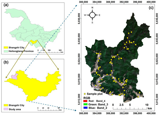
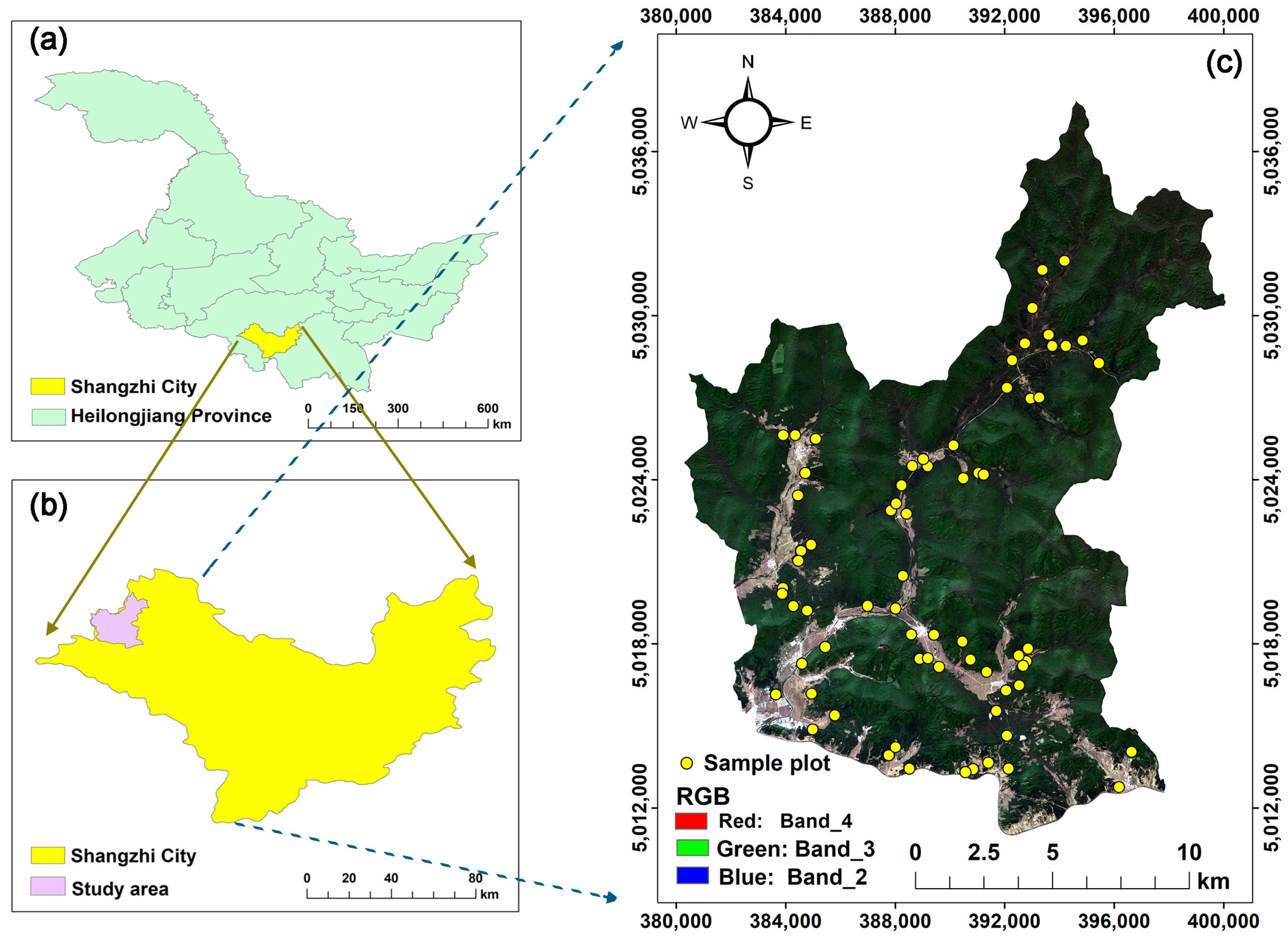
The study area is the Maoershan Forest Farm, situated between 127°29′E and 127°44′E, and 45°14′N and 45°29′N, in the southeastern region (Shangzhi city) of Heilongjiang Province. The mean elevation is approximately 300 m. The annual precipitation averages approximately 723 mm, with rainfall predominantly occurring from June to August; the average annual temperature is roughly 2.8 °C. The study area is dominated by natural secondary forests, with major tree species including Betula platyphylla, Pinus koraiensis, Quercus mongolica, Fraxinus mandshurica, and Ulmus spp. [27]. The prevailing soil type in the region is dark brown soil. The geographical location of the study area and the distribution of soil sample sites are shown in Figure 1.

Figure 1. Location of (a) Shangzhi City; (b) Maoershan Forest Farm; (c) SOC sample plots.

2.2. Remote Sensing Data

Sentinel-1 SAR and ZY1F Satellite Images

Sentinel-1 SAR works in the C-band, transmitting electromagnetic waves to the Earth autonomously, which can penetrate the vegetation, and therefore has a broad application prospect for the estimation of soil properties. The Sentinel-1 SAR images, obtained from the official website of ESA (https://www.esa.int/), are Level-1 Single Look Complex (SLC) products, including horizontal and vertical polarization. The polarization mode is VV + VH, and the spatial resolution is 10 m × 10 m. The cloudiness in the remote sensing image is below 1%, and the acquisition date is 2 September 2022. Sentinel-1 SAR imagery was preprocessed using Sentinel Application Platform [28], including thermal noise removal, orbit file correction, radiometric calibration, speckle filtering, and terrain correction, to derive incidence angle and backscatter information.

The Resource 01F satellite (ZY1F), an earth resource satellite jointly developed by China and Brazil, was launched on 26 December 2021. The satellite has a variety of payloads such as a multispectral imager, high-resolution camera, and infrared imager. This imagery captured on 9 September 2022 was acquired through the China Resources Satellite Application Center (http://data.cresda.cn). The specific parameters of AHSI are shown in Table 1. ZY1F satellite imagery was processed through radiometric calibration, atmospheric correction, and geometric refinement, followed by clipping to the region of interest to obtain the imagery for the study area.

Table 1. Resource-1 (ZF-1) hyperspectral data.

Spectral Range (nm)	Channel Number	Spectral Resolution (nm)	Spatial Resolution (m)
VNIR: 395–1040	76	10	30
SWNIR: 100–2480	90	20	30

2.3. The Reference Data of SOC

In June 2022, a stratified random sampling scheme was implemented across coniferous, broadleaf, and mixed forests. Twenty-five samples were initially taken from each stratum, yielding a final dataset of 67 soil samples after quality control. At each sampling point, one 1 m × 1 m quadrat was established. The soil samples were taken using a soil auger at the corners and center of the quadrat. According to GlobalSoilMap standard [29], the soil profile was divided into three layers: 0–5 cm, 5–15 cm, and 15–30 cm. Three specimens were obtained from each depth layer. Coordinates of each sampling location were documented via a handheld GPS device.

The soil samples were air-dried at ambient temperature in the laboratory. Following desiccation, discernible plant roots and organic detritus were eliminated, and the samples were subjected to sieving through a 1 mm mesh to reduce interference from organic matter in the SOC analysis. The soil organic carbon (SOC) content was determined using a carbon–nitrogen elemental analyzer. To reduce measurement error, each sample was measured three times, and the average value was recorded as the final SOC value for that point.

According to a previous study [30], the SOC content for the 0–30 cm layer was calculated as the average of the three individual layers (0–5 cm, 5–15 cm, and 15–30 cm). A statistical summary of SOC content across the different soil layers is presented in Table 2.

Table 2. Descriptive statistics of measured SOC content.

Soil Depth	SOC (g/kg)
	Min	Max	Mean	Median	Standard Deviation
0–5 cm	34.83	275.80	121.23	108.43	65.19
5–15 cm	32.59	121.50	59.04	51.03	21.24
15–30 cm	30.18	101.45	48.24	42.98	15.14

2.4. Auxiliary Datasets

In addition to the above remotely sensed data, this study also utilized auxiliary information to enhance the accuracy of forest SOC estimation, including elevation, soil moisture, and forest aboveground biomass (AGB) data. The 30 m resolution digital elevation model (DEM) data were obtained from the Geospatial Data Cloud platform (https://www.gscloud.cn). The AGB dataset was derived from previous research, which was estimated based on forest inventory data and predicted using a 1D-CNN model, achieving good accuracy, with an R² of 0.99 and an RMSE of 2.02 kg/ha [31]. Soil moisture data were obtained from the China Soil Moisture Dataset (https://doi.org/10.5194/essd-13-3239-2021), with a spatial resolution of 0.05° [32]. In addition, the 2024 forest inventory data, encompassing information on herbaceous plants, trees, and soils, were utilized to investigate the relationship between aboveground forest vegetation and soil carbon, with the goal of enhancing the accuracy of forest SOC estimation.

2.5. Method Overview

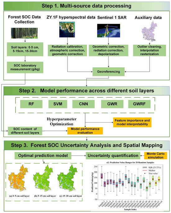
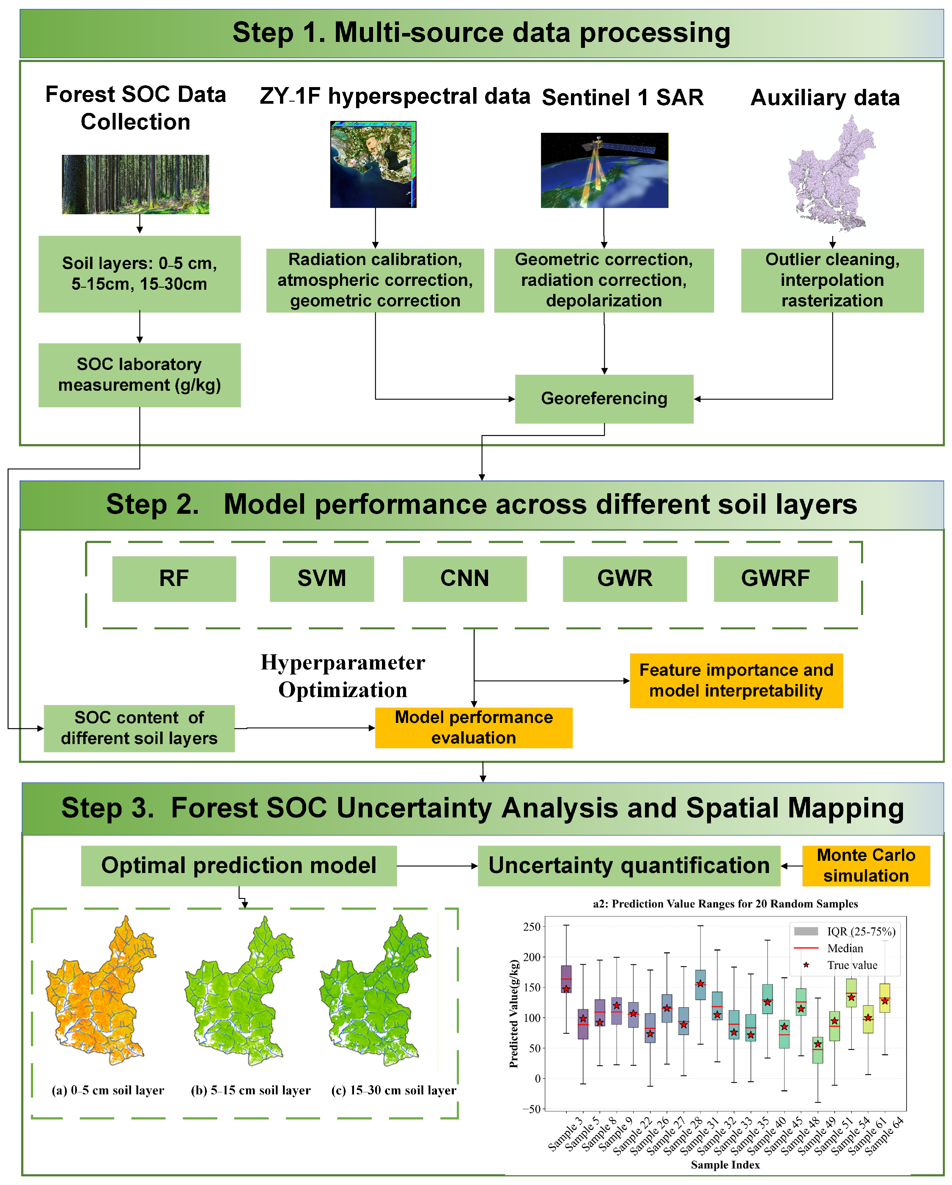
To improve the accuracy of SOC estimation under complex forest conditions, the following technical approach was adopted: (1) data collection and preprocessing, including hyperspectral satellite imagery, Sentinel-1 SAR data, and auxiliary datasets (topography, vegetation, and soil), followed by data correction and georeferencing; (2) development and evaluation of five prediction models—random forests, support vector machines, convolutional neural network, geographically weighted regression, and geographically weighted random forest—to assess performance across different soil layers and data sources; and (3) generating spatial distribution maps of SOC across different soil layers and assessing uncertainty in SOC estimation using a Monte Carlo approach integrated with machine learning. The overall workflow is illustrated in Figure 2.

Figure 2. The flowchart of this study.

2.6. Feature Extraction and Selection

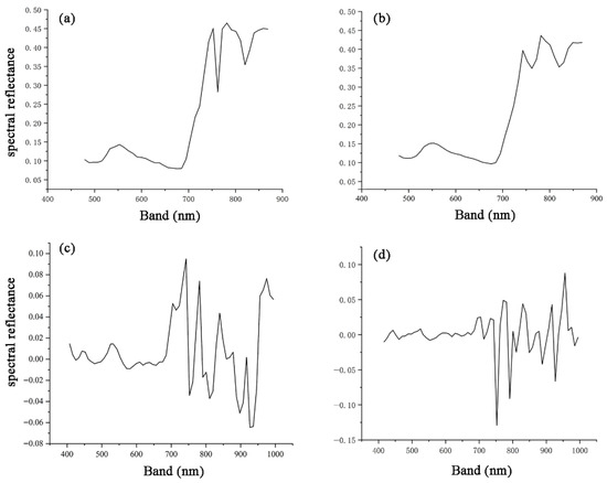
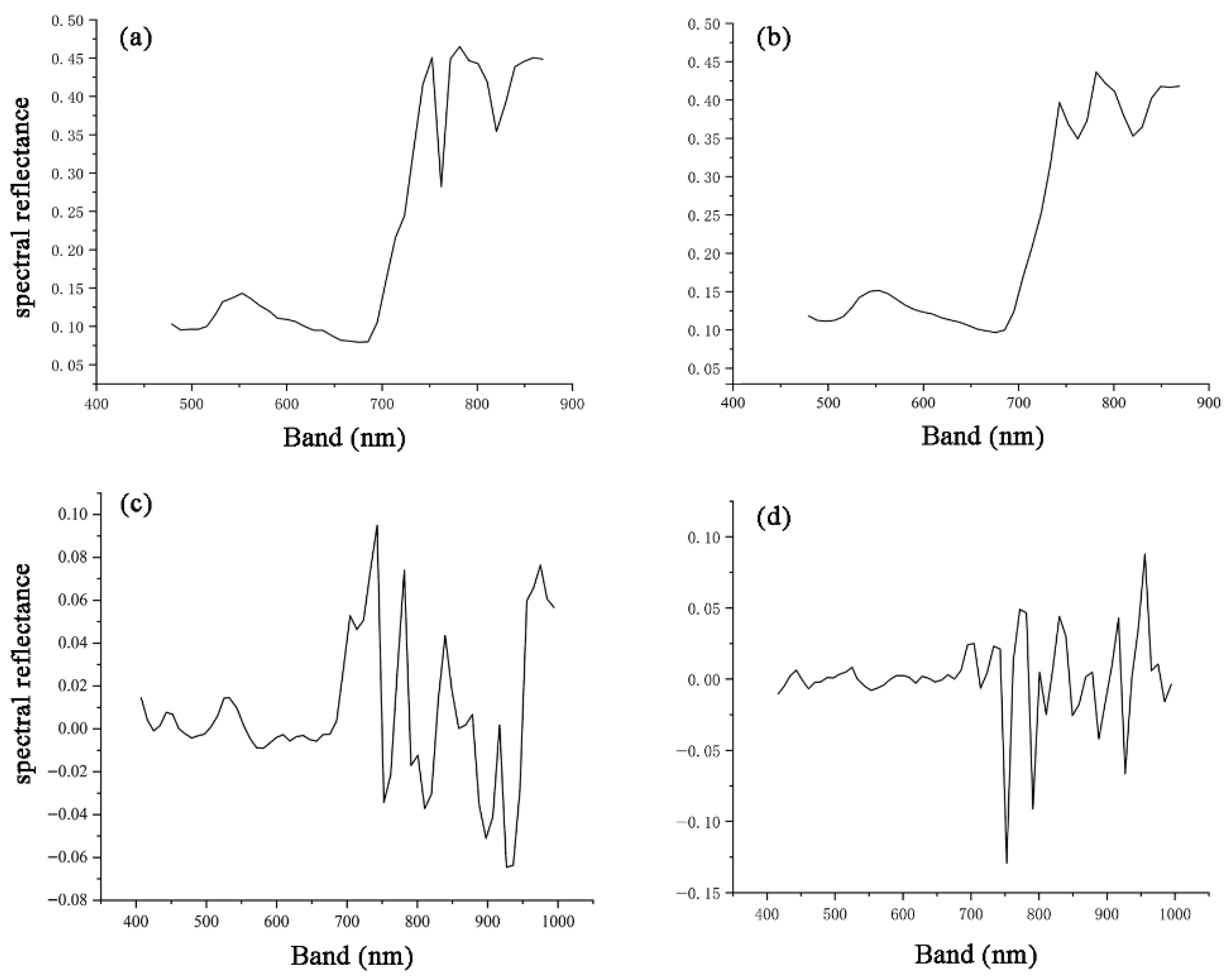
The derivations of the spectral curve can effectively describe the variation trends and dynamic processes of spectral data, which is beneficial for analyzing soil physicochemical properties [33]. Thus, the first-order derivative, the second-order derivative, and the reciprocal logarithmic transformation were applied to the hyperspectral imagery. The first-order derivative was employed to diminish noise and interference in the spectral curves and to extract distinctive information, while the second-order derivative was utilized to examine the nonlinear fluctuations in the spectral curves. As shown in Figure 3, spectral differentiation enhances the original spectral features, which is useful for emphasizing soil information. Equations for spectral differentiation are as follows:

$$R^{\prime }\left({\lambda }_i\right)={\displaystyle \frac{\left\{R\left({\lambda }_{i+1}\right)-R\left({\lambda }_{i-1}\right)\right\}}{2\mathrm{\Delta }\lambda }}$$

(1)

$$R^{″}\left({\lambda }_i\right)={\displaystyle \frac{\left\{R^{\prime }\left({\lambda }_{i+1}\right)-R^{\prime }\left({\lambda }_{i-1}\right)\right\}}{2\mathrm{\Delta }\lambda }}$$

(2)

where, R′ and R″ represent the first- and second-order derivatives of reflectance R, respectively.

Figure 3. The reflectance curve of ZY-1 imagery based on different processing methods. (a) Original band reflectance; (b) convolutionally smoothed band reflectance; (c) reflectance of first-order derivative; (d) reflectance of second-order derivative.

The 31 vegetation indices related to soil and vegetation were extracted. These indices indirectly reflect soil conditions by capturing information on vegetation health, canopy cover, and soil background characteristics through two primary pathways: (1) areas with higher vegetation productivity (indicated by higher VI values) typically receive greater litter inputs, enhancing surface soil organic carbon, and (2) canopy density, reflected in vegetation indices, influences understory microclimate and soil erosion rates, thereby affecting SOC dynamics [34]. Nine topographic factors were extracted to explore the influence of terrain factors on forest SOC. Detailed information is provided in Supplementary Table S1.

SAR backscatter signals, particularly in vertically vertical (VV) and vertically horizontal (VH) polarization modes, exhibit high sensitivity to surface soil moisture content, surface roughness, and canopy structure [14]^. Soil moisture directly regulates microbial activity and soil organic carbon (SOC) decomposition rates. Furthermore, SAR-derived signals indirectly reflect the drainage conditions and vegetation belt locations—well-drained slopes versus poorly drained depressions—factors that fundamentally govern organic matter accumulation patterns [16]. Finally, since soil organic carbon partially originates from litterfall and root renewal, areas with higher biomass typically receive greater organic matter inputs. Thus, this study extracted VV and VH polarization characteristics derived from SAR during growing and non-growing seasons. Due to the high dimensionality of features in hyperspectral data, dimensional catastrophe and overfitting are often triggered, resulting in the decrease in model accuracy with the increase in the number of features [35]. Feature selection can identify the relevant variables that are significant to the target variable, eliminate irrelevant variables, avoid model overfitting, and improve the model fitting effect. This study employed the SHapley Additive exPlanations (SHAP) method to evaluate feature importance and guide feature selection [36]. SHAP offers local interpretability by elucidating the prediction outcomes of individual samples, hence highlighting the rationale behind a model’s specific result. This is especially beneficial for elucidating “black box” models like machine learning or deep learning. In addition, SHAP values allow for the intuitive identification of features with strong influence on model predictions, as well as the detection of abnormal samples [36].

2.7. Models for Forest SOC Estimation

Various prediction models were conducted in this study for the forest SOC estimation, including random forests (RFs) [37], support vector machines (SVMs) [38], CNNs [39], and the GWRF model. The RF and SVM models are traditional machine learning models used for nonlinear prediction tasks. The CNN model in this study contains five convolutional layers with a window size of 3, two maximum pooling layers with a step size of 3, a flat layer and a fully connected layer.

In traditional regression models, the regression coefficients are assumed to be the same in all areas. However, many phenomena exhibit different patterns in different regions, thus requiring the regression coefficients to vary independently for each location. Geographically weighted regression (GWR) is a method used to process geospatial data [22]. The GWR formula is as follows:

$$y_i={\beta }_0\left(u_i,v_i\right)+{\sum }_{k=1}^p{\beta }_k\left(u_i,v_i\right)x_{ik}+{ϵ}_i$$

(3)

$(u_i,v_i)$ is the geographic coordinate at location i; ${\beta }_0(u_i,v_i)$ is the local intercept at location i; ${\beta }_k\left(u_i,v_i\right)$ is the local regression coefficient for the kth independent variable at location i; and ${ϵ}_i$ is the model residual.

However, GWR models have several challenges when dealing with complex, high-dimensional data. Geographically weighted random forest (GWRF) is a statistical technique that combines spatially localized modeling and integrated learning methods to deal with spatial heterogeneity by taking into account the spatial location of samples in the prediction process [40]. GWRF does not have a specific model form. For ease of understanding, we simplified GWRF into the following form:

$${\widehat{y}}_i=RF(u_i,v_i)\left(x_i\right)$$

(4)

$RF(u_i,v_i)$ represents the locally trained random forest model at coordinates $(u_i,v_i)$; $\left(x_i\right)$ denotes the feature set at geographic location i.

Due to the large number of model hyperparameters, this study used a random search strategy for hyperparameter optimization [41]. The specific optimization parameters are shown in Supplementary Materials Table S2. Due to the small sample size of this study, Leave-One-Out Cross-Validation (LOOCV) was used to evaluate the model accuracy [42]. The accuracy metrics used were the coefficient of determination (R²), Root Mean Square Error (RMSE) and Relative Root Mean Square Error (rRMSE).

2.8. Uncertainty Quantification of Forest SOC Estimation

An uncertainty quantification method combining Monte Carlo simulation with machine learning was developed to quantify the uncertainty in forest SOC estimation. Through repeated iterative simulations, the Monte Carlo algorithm simplifies complex mathematical relationships and generates statistical measures of uncertainty, offering a new perspective for uncertainty quantification in machine learning models. The specific implementation steps included: (1) model construction; (2) adoption of a bootstrap sampling strategy combined with randomized model hyperparameters to establish appropriate perturbation distributions; (3) a total of 1000 Monte Carlo simulations to evaluate result convergence; and (4) the standard deviation (STD) and coefficient of variation (CV) were computed as uncertainty metrics to reflect the dispersion—and thus the uncertainty—of the estimated values.

3. Results

3.1. Feature Importance Ranking

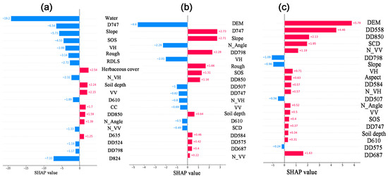
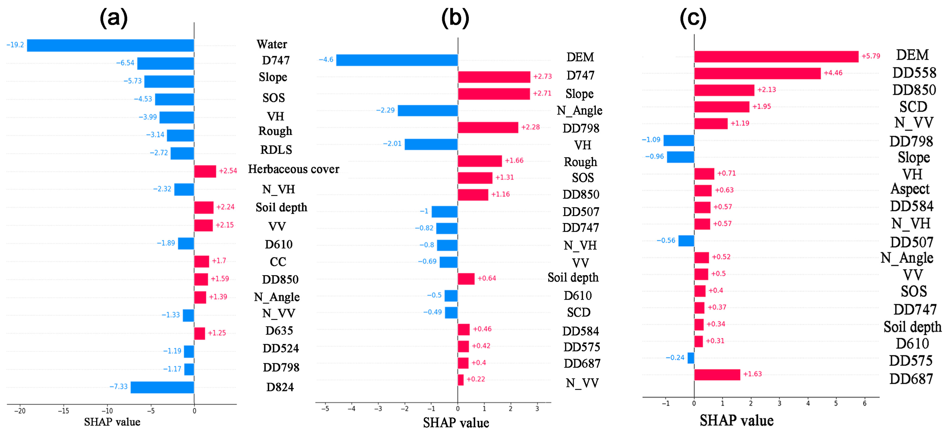
Figure 4 presents the feature importance ranking using the SHAP method for estimating forest SOC of different soil depths, highlighting the top 20 features. For the soil depths of 0–5 cm, environmental variables—such as terrain, soil depth, and vegetation cover—play a critical role, with soil moisture content (i.e., water) emerging as the most influential factor in forest SOC estimation. For soil depths of 5–15 cm and 15–30 cm, topography characteristics exhibit considerable significance, with elevation (DEM) being the most prominent factor.

Figure 4. Feature importance ranking for different soil depths. (a), (b), and (c) are the overall importance of all samples for soil depths of 0–5 cm, 5–15 cm, and 15–30 cm, respectively. Note: Water: soil moisture content; Dxxx: first-order derivative of the given (xxx band) wavelength; DDxxx: second-order derivative of the given (xxx band) wavelength; Slope: slope derived from digital elevation model; SOS: slope gradient; VH: VH polarization feature; Rough: surface roughness; RDLS: terrain undulation; N_VH: VH polarization feature during the non-growing season; VV: VV polarization feature; CC: canopy cover; N_Angle: aspect angle during the non-growing season; N_VV: VV polarization feature during the non-growing season; SCD: surface cutting depth; DEM: digital elevation model.

Sentinel-1–derived polarization metrics, particularly VH and VV, also exhibit high importance. This suggests that the C-band synthetic aperture radar onboard Sentinel-1 possesses a certain penetration capability in natural secondary forests and can, to some extent, capture variations in soil physicochemical properties. Meanwhile, the first- and second-order derivatives derived from the ZY-1 hyperspectral satellite data contribute to forest SOC estimation, whereas the raw spectral features exhibit relatively low importance; the red and near-infrared bands were the dominant contributors among the first- and second-order derivative features.

3.2. Prediction Model Comparison Based on Multi-Sourced Data

This study assessed the estimation accuracy of five models (RF, SVM, CNN, GWR, and GWRF) for forest soil organic carbon, emphasizing model performance and their ability to address spatial heterogeneity using three datasets (Sentinel 1, ZY-1F, and Sentinel 1 + ZY-1F). Supplementary Materials Table S3 shows the estimated SOC values at different depths. The model performance for topsoil (i.e., 0–5 cm) surpasses that of deeper soil (i.e., 5–15 cm, and 15–30 cm). As soil depth increases, the predictive performance of all models declines across all data sources, reflecting the inherent difficulty of remote sensing signals in penetrating deep soil layers. Additionally, in shallow soil layers, Sentinel-1 synthetic aperture radar data demonstrated superior performance due to its enhanced penetration capability for acquiring soil information.

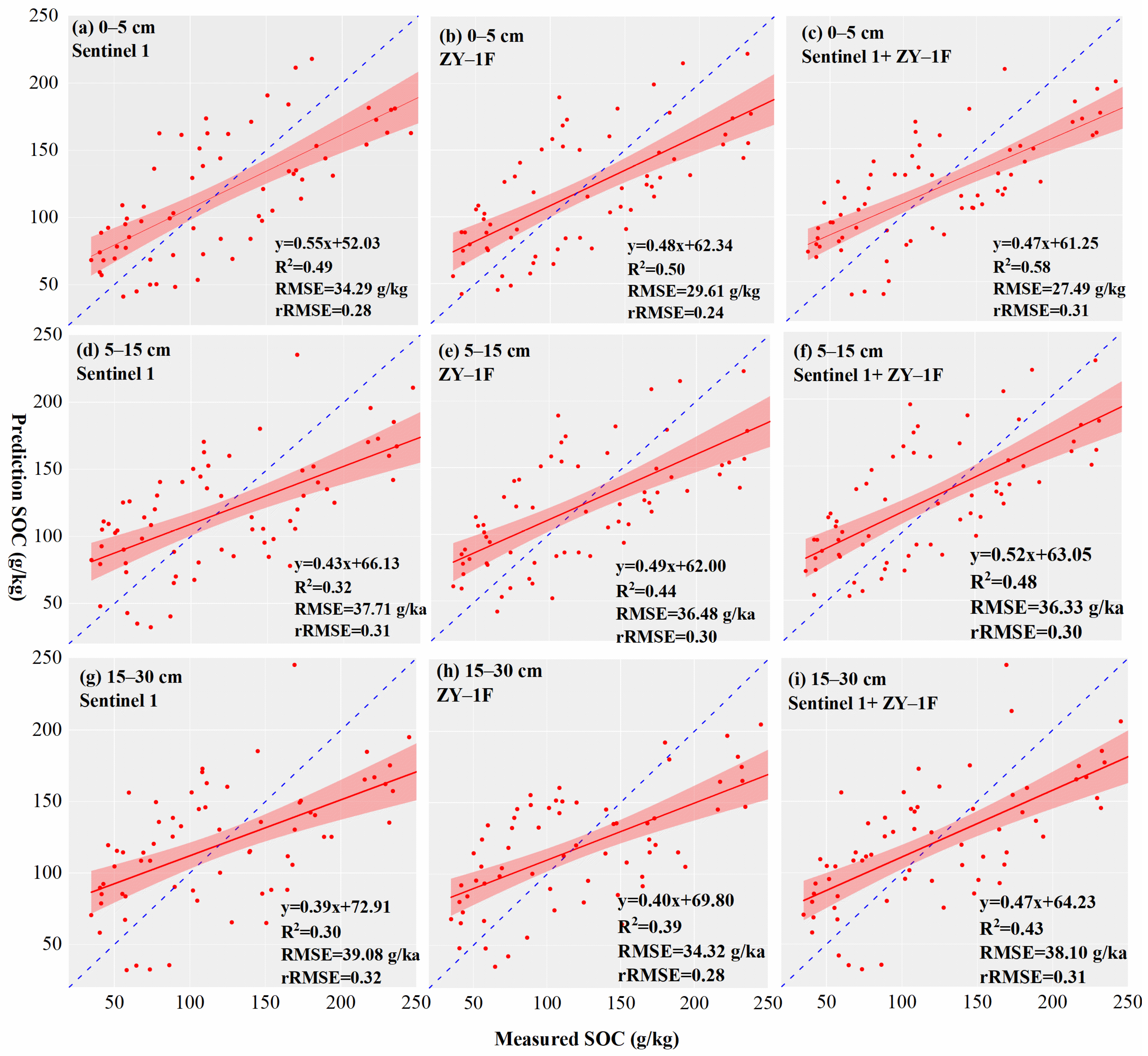
Supplementary Materials Table S3 shows that the GWRF model achieved the best performance, attaining the highest accuracy (R² = 0.58, RMSE = 27.49 g/kg, rRMSE = 0.31) when integrating multi-source data from Sentinel-1 and ZY-1F and significantly outperforming the other algorithms with other single data (i.e., only Sentinel-2 or ZY-1F). The GWR maintained R² values above 0.35 across single-source datasets, with RMSE values lower than those of RF and other algorithms, indicating its effectiveness in capturing spatial heterogeneity. Traditional machine learning approaches (RF, SVM, and CNN) showed relatively weaker predictive capability (R² generally < 0.3). Regarding the influence of data sources, multi-source data fusion (Sentinel-1 + ZY-1F) substantially improved the accuracy of all algorithms (R² increased by approximately 7.40% to 15.52% in 0–5 cm soil layer), confirming the complementary value of integrating passive and active remote sensing data.

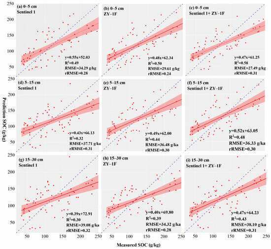
Figure 5 displays the scatter plot of GWRF model predictions, illustrating that multi-source remote sensing data integration enhances estimation accuracy compared to a single data source. In the 0–5 cm soil layer, the integration of multi-source data increased R² by 15.52%, reduced RMSE by 24.74%, and lowered rRMSE by 9.67% compared to using Sentinel-1 data alone. When using the same data source, the model’s fitting accuracy exhibited a consistent decline as soil depth increased. Additionally, the SOC values exhibit a broad range (20–250 g/kg), and the model fitting is significantly impacted by the high values, which presents a substantial challenge for forest SOC estimation.

Figure 5. Scatter plots of estimated versus measured forest SOC using the GWRF model based on multi-source data for different soil depths: (a), (b), and (c) represent Sentinel-1, ZY-1F, and Sentinel-1 + ZY-1F in the 0–5 cm soil layer, respectively; (d), (e), and (f) represent Sentinel-1, ZY-1F, and Sentinel-1 + ZY-1F in the 5–15 cm soil layer, respectively; (g), (h), and (i) represent Sentinel-1, ZY-1F, and Sentinel-1 + ZY-1F in the 15–30 cm soil layer, respectively. The red area represents the 95% confidence interval. The blue dash line represents the function y = x.

3.3. Uncertainty Analysis

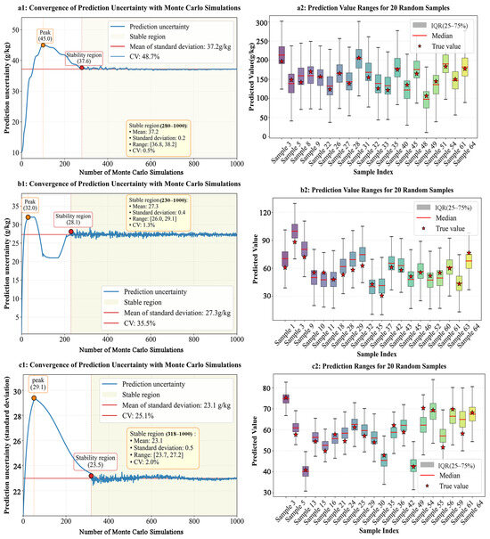
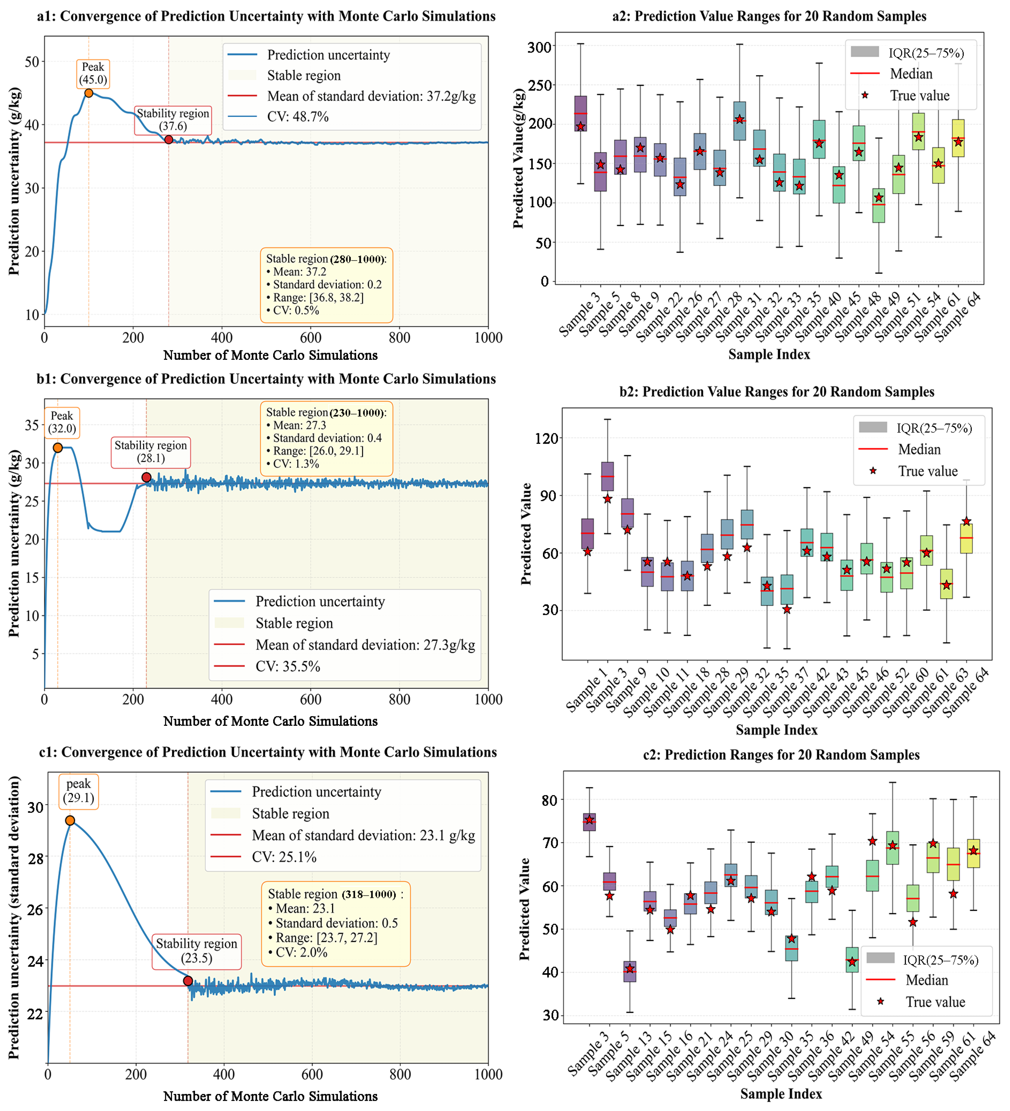
Figure 6 illustrates the uncertainty in SOC estimation across different soil depths using the optimal model (i.e., GWRF) combined with the Monte Carlo algorithm. When the number of simulations was low (<100), uncertainty increased rapidly due to the strong influence of extreme values. As the number of MC simulations increased, the uncertainty of the prediction results gradually stabilized (after approximately 230 to 318 simulations), with the coefficient of variation during the stable phase ranging between 0.5% and 2.0%.

Figure 6. Uncertainty in forest SOC estimation using GWRF across different soil depths. (a1–c1) represent the curves of uncertainty in prediction results as the number of MC simulations increases for soil layers at 0–5 cm, 5–15 cm, and 15–30 cm, respectively. The white- and yellow-background boxes represent the overall MC simulation statistics and the stability region statistics of the uncertainty curves, respectively. (a2–c2) represent boxplots of predicted 20 random samples in soil layers of 0–5 cm, 5–15 cm, and 15–30 cm, respectively. IQR represents the interquartile range.

An unexpected phenomenon was observed from Figure 6(a1–c1): as soil depth increased, the uncertainty of the predictions gradually decreased, with the relative uncertainty (coefficient of variation) declining from 48.7% to 25.1%. Figure 6(a2–c2) shows the distribution of the predicted results for 20 random samples in the 0–5 cm, 5–15 cm, and 15–30 cm soil layers, respectively. Previous studies [43,44] have demonstrated that the contribution of model residual uncertainty significantly affects the overall results, primarily due to low model accuracy leading to high residual uncertainty. As soil depth increased, the absolute uncertainty (measured by standard deviation) of GWRF predictions gradually decreased, from 37.2 g/kg in the 0–5 cm layer to 23.1 g/kg in the 15–30 cm layer (Figure 6(a1–c1)). This pattern is primarily attributable to the narrower range and lower mean values of SOC in deeper soil layers (Table 2), which inherently constrain the possible variation in predicted values. Importantly, the decreasing absolute uncertainty does not contradict the finding that prediction accuracy (R² and RMSE) declined with depth; accuracy reflects the magnitude of prediction errors relative to measured values, whereas uncertainty reflects the dispersion of repeated predictions. In deeper layers, the model consistently underperforms (low accuracy) but does so with greater stability (low uncertainty) due to the constrained SOC range.

3.4. Spatial Distribution of the Forest SOC Across Different Soil Depths

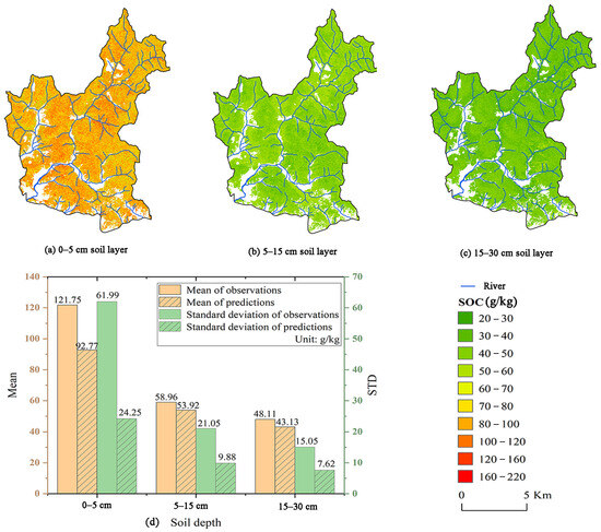
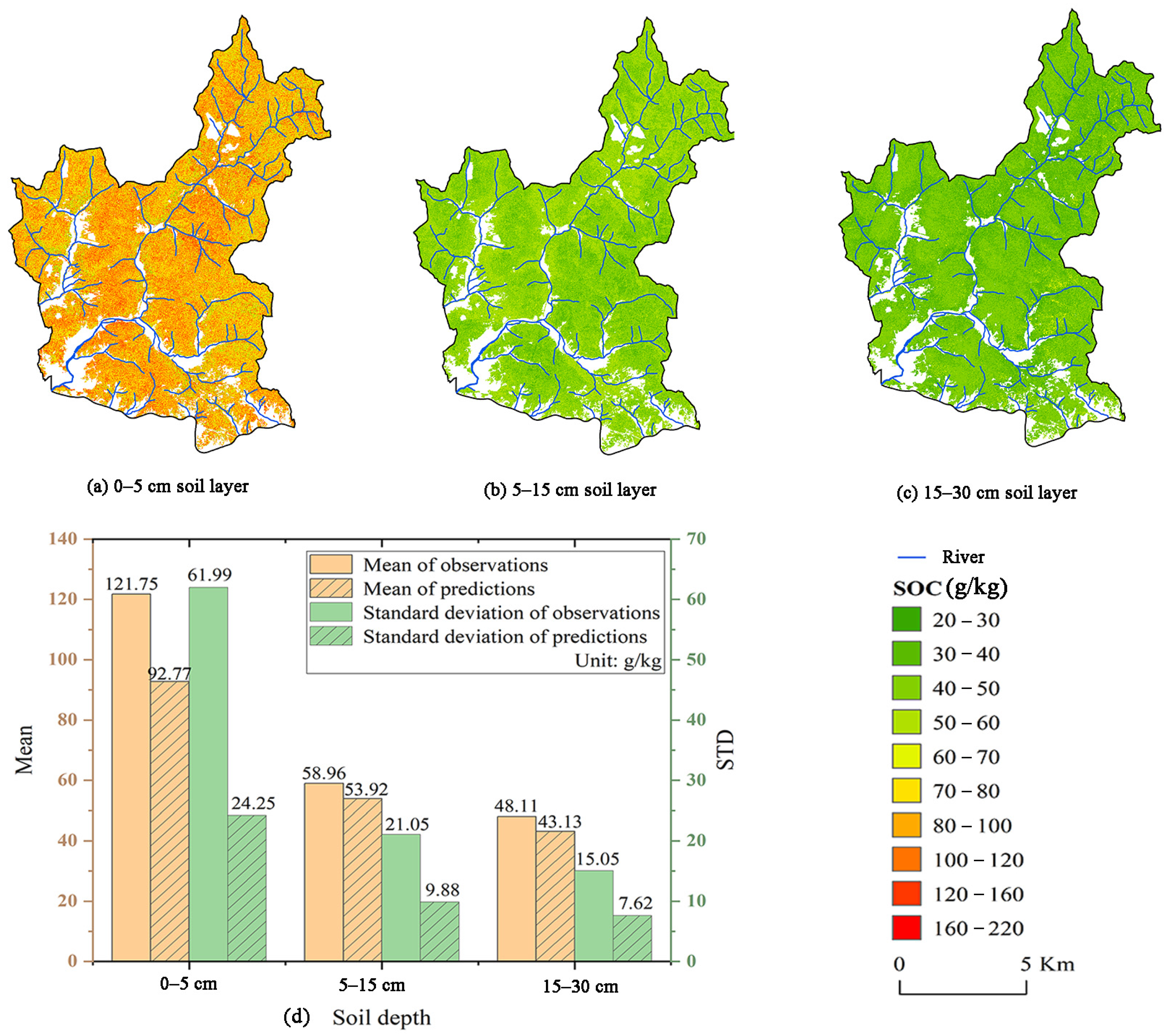
Figure 7 shows the spatial distribution of the SOC estimation using GWRF and multi-source data at different depths of Maoershan forest farm. For the 0–5 cm topsoil layer (Figure 7a), forest SOC content was primarily concentrated between 80 and 160 g/kg. For the 5–15 cm soil layer (Figure 7b), forest SOC content was concentrated between 40 and 70 g/kg, with a spatial distribution similar to that of the 0–5 cm soil layer. For the 15–30 cm soil layer (Figure 7c), SOC content was primarily concentrated between 20 and 60 g/kg. Figure 7d shows that the GWRF model underestimated the mean SOC at all soil depths, with the topsoil exhibiting the most significant underestimation (121.75 g/kg vs. 92.77 g/kg) and the subsequent soil layers significantly reduced in underestimation (e.g., 48.11 g/kg vs. 43.13 g/kg).

Figure 7. Spatial distribution of SOC estimation using GWRF and multi-source data in different soil layers. (a) 0–5 cm soil layer; (b) 5–15 cm soil layer; (c) 15–30 cm soil layer; (d) comparison of predicted and observed SOC.

4. Discussion

4.1. The Role of Various Data Sources in Forest SOC Estimation

This study aims to investigate the effects of different models and data sources on SOC estimation in complex natural forests, thereby providing a basis for improving forest SOC estimation accuracy. Compared to SOC estimation in bare land and cropland, forest SOC estimation presents a greater challenge due to high vegetation coverage [45,46,47]. The dense canopy limits the penetration of remote sensing signals, reducing estimation accuracy. Therefore, identifying appropriate data sources and derived effective features to establish a robust relationship with forest SOC is critical.

According to the SHAP feature analysis (see Figure 4), Sentinel-1 is sensitive to surface roughness, moisture, and vegetation structure and can penetrate cloud cover [14], while ZY-IF is sensitive to moisture and vegetation biochemical properties. These characteristics serve as indicators of the ecological processes influencing soil organic carbon accumulation [48]. Surface vegetation attributes, including canopy and herbaceous cover, substantially affect topsoil SOC, while their effect on deep soil SOC is minimal. Topographic factors such as slope, aspect, and elevation play a critical role in predicting forest SOC, consistent with findings from previous studies [10,49,50], particularly regarding the pronounced influence of aspect. As a key topographic variable, aspect indirectly affects SOC accumulation by altering soil moisture and thermal conditions through its impact on light intensity and duration [51].

Moreover, spatial distribution maps (Figure 7) reveal a clear association between forest SOC and river networks. River areas, characterized by abundant moisture and high productivity, experience substantial litter input [45]. Coupled with anaerobic conditions that suppress decomposition, these factors promote organic carbon accumulation, establishing soils in such areas as significant carbon sinks [52]. Conversely, intensive human activities within watersheds can trigger rapid carbon release, potentially offsetting sequestration [53]. Therefore, targeted monitoring of carbon dynamics around rivers is essential for understanding the broader carbon cycle.

The study found that the first- and second-order spectral derivatives had a significant effect on forest SOC estimation. This is because spectral derivatives are less sensitive to noise, thereby reducing background interference and enhancing spectral sensitivity. Feature importance ranking further indicated that the red and near-infrared bands played a crucial role in SOC estimation, consistent with the results of previous studies [54,55]. This suggests that the red-edge and near-infrared bands can indirectly capture the relationship between key forest canopy/surface biophysical features and the accumulation and distribution of SOC [34]. Highly productive forests, characterized by strong red-light absorption due to chlorophyll activity, exhibit increased SOC content through enhanced inputs of litter and root exudates [56]. The study also found that the correlation between SOC and the red/NIR bands differs across soil depths (Figure 4). In the 0–5 cm layer, the correlation is predominantly positive, whereas it gradually shifts toward a negative trend with increasing soil depth. This pattern likely results from the effects of ecological processes (e.g., carbon input dynamics and vertical SOC differentiation) and the technical limitations of remote sensing penetration.

4.2. The Model Comparison in Estimating Forest SOC

Although machine learning models (e.g., random forests, support vector machines, and deep learning models) are capable of capturing complex nonlinear relationships between environmental factors and SOC, they did not achieve satisfactory predictive performance in this study. A possible reason is the complex canopy structure of nature forests, which blocks most signals and limits the capacity of capturing soil information. This also explains why model accuracy is generally higher in croplands and grasslands than in forested areas [34,57].

As global models, the RF, SVM, and CNN models learn a uniform and fixed input-output relationship across the entire study area. When the relationship between forest SOC and remote sensing features exhibits spatial heterogeneity, these models converge to an “averaged” pattern, which causes increased prediction bias at the local scale. Compared with the RF and SVM models, the GWR model improved prediction accuracy by more than 30% (Figure 5), suggesting that incorporating spatial relationships can substantially enhance the estimation of forest SOC. GWR applies local regression analysis [58], allowing model parameters to vary with geographic location and thereby effectively accounting for the spatial heterogeneity of SOC distribution. However, the GWR model relies on strong linearity assumptions, making it less effective in capturing complex nonlinear associations, and its computational complexity increases markedly with larger datasets [58]. By incorporating geographical weighting, GWRF optimally integrates the strengths of both GWR and RF and achieves localized modeling while fully leveraging the complex, nonlinear synergies and interactions between Sentinel-1 and ZY-1F features [40]. This study validated the GWRF model’s superiority in estimating forest SOC compared to the RF or GWR models alone across all data sources due to its capacity to concurrently address spatial heterogeneity and nonlinear relationships.

4.3. Analysis Uncertainty of Soil Organic Carbon Estimation

GWRF combines geographically weighted regression and random forests. While this combination enhances predictive power, it also introduces additional sources of uncertainty: (1) the choice of spatial weighting functions (e.g., Gaussian kernel, bilinear kernel) and their bandwidth parameters directly influence the delineation of local neighborhoods; (2) the hyperparameter configurations of each local RF model may vary spatially, leading to spatial heterogeneity in model behavior; and (3) spatial variations in local sample size—in sparsely sampled areas, the stability of local RF models decreases significantly [40].

The core strength of GWRF lies in capturing spatial non-stationarity, but this is also the primary source of its uncertainty. When the study area exhibits strong spatial heterogeneity, limited sample sizes may fail to adequately represent all local conditions, resulting in high prediction uncertainty in certain areas (e.g., regions with complex topography or dense vegetation). In this study, the prediction uncertainty of GWRF for the 0–5 cm surface soil layer was 37.2 g/kg, decreasing with increasing depth; this pattern may be related to the stronger spatial variability and environmental sensitivity of surface SOC.

Compared with existing studies, the prediction uncertainty of GWRF in this study falls within an acceptable range. For example, Zhang et al. found that the relative uncertainty in their study of soil organic carbon ranged from 9.10% to 22.9% [59]. Dvorakova et al. found that the average uncertainty was 14 g C kg⁻¹ using Sentinel-2 data in combination with vegetation indices [60]. This is consistent with our observations—although absolute uncertainty exists, the relative advantage of GWRF remains stable.

However, several limitations remain: (1) A key finding of this study is that data distribution significantly influences prediction uncertainty; therefore, future research should critically evaluate sample size and spatial distribution, providing valuable guidance for field data collection. Research has shown that the SVM model is the least sensitive to sample size, achieving reasonable performance even with limited samples, while ensemble methods like RF and XGBoost continue to improve with increasing sample size [61]. This explains why the SVM model performed reasonably well in our study despite the limited sample size (67 plots) yet was still outperformed by GWRF—suggesting that the spatial information gain in GWRF can partially compensate for sample size limitations. Research on digital soil mapping indicates that the size of the training dataset directly influences the level of model uncertainty [62]; a large training dataset can significantly reduce model uncertainty compared to a small one. However, due to sampling cost constraints, this study utilized 67 samples. The limited number and uneven spatial distribution of soil samples represent a notable limitation of this study. The stratified random sampling design partially mitigated this issue by ensuring representation across major forest types, but the spatial coverage remains constrained by accessibility constraints in mountainous terrain. This limitation may affect the model’s ability to fully capture the spatial heterogeneity of SOC, particularly in under-sampled areas.

(2) Further efforts should be directed toward integrating advanced deep learning models with spatial statistical methods. For example, combining convolutional neural networks (CNNs) with geographically weighted regression (GWR) offers a promising avenue for capturing both nonlinear associations and spatial non-stationarity. Embedding spatial positional relationships into CNN convolutional layers could lead to the development of algorithms with improved predictive capability, providing more powerful tools for forest SOC estimation under complex canopy conditions [63].

5. Conclusions

This study introduced a ForSOC-UA framework that integrates forest SOC estimation by GWRF and associated uncertainty quantification via Monte Carlo methods, utilizing hyperspectral, synthetic aperture radar, and environmental data. Feature importance analysis indicated that soil moisture and topographic variables were dominant drivers of SOC distribution because they modulate redistribution of water, nutrients, and litter, while Sentinel-1 polarization features and hyperspectral derivatives in the red and near-infrared bands also played important roles in forest SOC estimation because spectral derivatives capture canopy productivity that indirectly reflects carbon inputs to soil. In the 0–5 cm soil layer, the GWRF approach was consistently found to achieve the highest accuracy (R² = 0.58, RMSE = 27.49 g/kg, rRMSE = 0.31) using the integrated Sentinel 1 and ZY-1F images, significantly outperforming conventional machine learning models (i.e., RF, SVM, and CNN) with an R² improvement ranging from 13.8% to 53.4%. This improvement is because GWRF takes into account both spatial instability and complex nonlinear relationships. An additional finding was that the relative uncertainty gradually decreased with increasing soil depth—from 48.7% to 25.1%. This phenomenon is related to the vertical distribution of soil organic carbon input and the reduction in the range of deep SOC values.

This study proposes the ForSOC-UA framework, which integrates SOC estimation and uncertainty analysis based on machine learning, focusing on the complex natural secondary forest environment, and reveals the changing patterns of SOC estimation uncertainty in different depth soil layers. This framework supports refined carbon sink accounting and offers methodological and modeling references for the assessment of regional-scale forest soil carbon stocks and sequestration potential.

References

- Mo, L.; Zohner, C.M.; Reich, P.B.; Liang, J.; de Miguel, S.; Nabuurs, G.; Renner, S.S.; van den Hoogen, J.; Araza, A.; Herold, M.; et al. Integrated global assessment of the natural forest carbon potential. Nature 2023, 624, 92–101. [Google Scholar] [CrossRef] [Scilit]
- Raza, S.; Zamanian, K.; Ullah, S.; Kuzyakov, Y.; Virto, I.; Zhou, J. Inorganic carbon losses by soil acidification jeopardize global efforts on carbon sequestration and climate change mitigation. J. Clean. Prod. 2021, 315, 128036. [Google Scholar] [CrossRef] [Scilit]
- Angelopoulou, T.; Tziolas, N.; Balafoutis, A.; Zalidis, G.; Bochtis, D. Remote Sensing Techniques for Soil Organic Carbon Estimation: A Review. Remote Sens. 2019, 11, 676. [Google Scholar] [CrossRef] [Scilit]
- Li, T.; Cui, L.; Kuhnert, M.; McLaren, T.I.; Pandey, R.; Liu, H.; Wang, W.; Xu, Z.; Xia, A.; Dalal, R.C.; et al. A comprehensive review of soil organic carbon estimates: Integrating remote sensing and machine learning technologies. J. Soils Sediments 2024, 24, 3556–3571. [Google Scholar] [CrossRef] [Scilit]
- Xie, Z.B.; Zhu, J.G. Soil organic carbon stocks in china and changes from 1980s to 2000s. Glob. Change Biol. 2007, 13, 1989. [Google Scholar] [CrossRef] [Scilit]
- Post, W.M.; Emanuel, W.R.; Zinke, P.J.; Stangenberger, A.G. Soil carbon pools and world life zones. Nature 1982, 298, 156–159. [Google Scholar] [CrossRef] [Scilit]
- Smith, P.; Powlson, D.S.; Smith, J.U.; Falloon, P.; Coleman, K. Meeting Europe’s climate change commitments: Quantitative estimates of the potential for carbon mitigation by agriculture. Glob. Change Biol. 2000, 6, 525–539. [Google Scholar] [CrossRef] [Scilit]
- Wieder, W.R.; Bonan, G.B.; Allison, S.D. Global soil carbon projections are improved by modelling microbial processes. Nat. Clim. Change 2013, 3, 909–912. [Google Scholar] [CrossRef] [Scilit]
- Sun, W.; Liu, X. Review on carbon storage estimation of forest ecosystem and applications in China. For. Ecosyst. 2020, 7, 4. [Google Scholar] [CrossRef] [Scilit]
- Hamzehpour, N.; Shafizadeh-Moghadam, H.; Valavi, R. Exploring the driving forces and digital mapping of soil organic carbon using remote sensing and soil texture. Catena 2019, 182, 104141. [Google Scholar] [CrossRef] [Scilit]
- Aburaed, N.; Alkhatib, M.Q.; Marshall, S.; Zabalza, J.; Ahmad, H.A. A Review of Spatial Enhancement of Hyperspectral Remote Sensing Imaging Techniques. IEEE J. Sel. Top. Appl. Earth Observ. Remote Sens. 2023, 16, 2275–2300. [Google Scholar] [CrossRef] [Scilit]
- Odebiri, O.; Odindi, J.; Mutanga, O. Basic and deep learning models in remote sensing of soil organic carbon estimation: A brief review. Int. J. Appl. Earth Obs. Geoinf. 2021, 102, 102389. [Google Scholar] [CrossRef] [Scilit]
- Shafizadeh-Moghadam, H.; Minaei, F.; Talebi-khiyavi, H.; Xu, T.; Homaee, M. Synergetic use of multi-temporal Sentinel-1, Sentinel-2, NDVI, and topographic factors for estimating soil organic carbon. Catena 2022, 212, 106077. [Google Scholar] [CrossRef] [Scilit]
- Santos, E.P.D.; Moreira, M.C.; Fernandes-Filho, E.I.; Demattê, J.A.M.; Dionizio, E.A.; Silva, D.D.D.; Cruz, R.R.P.; Moura-Bueno, J.M.; Santos, U.J.D.; Costa, M.H. Sentinel-1 Imagery Used for Estimation of Soil Organic Carbon by Dual-Polarization SAR Vegetation Indices. Remote Sens. 2023, 15, 5464. [Google Scholar] [CrossRef] [Scilit]
- Wang, Z.; Wu, W.; Liu, H. Spatial Estimation of Soil Organic Carbon Content Utilizing PlanetScope, Sentinel-2, and Sentinel-1 Data. Remote Sens. 2024, 16, 3268. [Google Scholar] [CrossRef] [Scilit]
- Gao, G. Statistical modeling of SAR images: A survey. Sensors 2010, 10, 775–795. [Google Scholar] [CrossRef] [Scilit]
- Zhang, Y.; Hartemink, A.E.; Huang, J.; Townsend, P.A. Synergistic use of hyperspectral imagery, Sentinel-1 and LiDAR improves mapping of soil physical and geochemical properties at the farm-scale. Eur. J. Soil Sci. 2021, 72, 1690–1717. [Google Scholar] [CrossRef] [Scilit]
- Sitaula, B.K.; Bajracharya, R.M.; Singh, B.R.; Solberg, B. Factors affecting organic carbon dynamics in soils of Nepal/Himalayan region—A review and analysis. Nutr. Cycl. Agroecosyst. 2004, 70, 215–229. [Google Scholar] [CrossRef] [Scilit]
- Xu, S.; Sheng, C.; Tian, C. Changing soil carbon: Influencing factors, sequestration strategy and research direction. Carbon Balance Manag. 2020, 15, 2. [Google Scholar] [CrossRef] [Scilit]
- Baveye, P.C.; Laba, M. Moving away from the geostatistical lamppost: Why, where, and how does the spatial heterogeneity of soils matter? Ecol. Model. 2015, 298, 24–38. [Google Scholar] [CrossRef] [Scilit]
- Odebiri, O.; Mutanga, O.; Odindi, J.; Naicker, R.; Masemola, C.; Sibanda, M. Deep learning approaches in remote sensing of soil organic carbon: A review of utility, challenges, and prospects. Environ. Monit. Assess. 2021, 193, 802. [Google Scholar] [CrossRef] [Scilit] [PubMed]
- Zeng, C.; Yang, L.; Zhu, A.; Rossiter, D.G.; Liu, J.; Liu, J.; Qin, C.; Wang, D. Mapping soil organic matter concentration at different scales using a mixed geographically weighted regression method. Geoderma 2016, 281, 69–82. [Google Scholar] [CrossRef] [Scilit]
- Lu, B.; Ge, Y.; Qin, K.; Zheng, J. A review on geographically weighted regression. Geomat. Inf. Sci. Wuhan Univ. 2020, 45, 1356–1366. [Google Scholar]
- Zhou, Y.; Wei, G.; Wang, Y.; Wang, B.; Quan, Y.; Wu, Z.; Liu, J.; Bian, S.; Li, M.; Fan, W. Estimating regional forest carbon density using remote sensing and geographically weighted random forest models: A case study of mid-to high-latitude forests in China. Forests 2025, 16, 96. [Google Scholar] [CrossRef] [Scilit]
- Ma, Y.; Im, J.; Zhen, Z.; Zhao, Y. A framework for upscaling aboveground biomass from an individual tree to landscape level and qualifying the multiscale spatial uncertainties for secondary forests. Geo-Spat. Inf. Sci. 2025, 28, 97–116. [Google Scholar] [CrossRef] [Scilit]
- Hammersley, J. Monte Carlo Methods; Springer: Berlin/Heidelberg, Germany, 2013. [Google Scholar]
- Zhao, Y.; Ma, Y.; Quackenbush, L.J.; Zhen, Z. Estimation of Individual Tree Biomass in Natural Secondary Forests Based on ALS Data and WorldView-3 Imagery. Remote Sens. 2022, 14, 271. [Google Scholar] [CrossRef] [Scilit]
- Sheode, M.; Dharavath, K. Sentinel Application Platform (SNAP) as a Tool for SAR Interferometry to Detect Landslides; Sarkar, R., Maheshwari, B.K., Kumar, A., Eds.; Springer: Singapore, 2025; pp. 353–362. [Google Scholar]
- Padarian, J.; Minasny, B.; McBratney, A.B. Chile and the Chilean soil grid: A contribution to GlobalSoilMap. Geoderma Reg. 2017, 9, 17–28. [Google Scholar] [CrossRef] [Scilit]
- Hengl, T.; Mendes, D.J.J.; Heuvelink, G.B.; Ruiperez, G.M.; Kilibarda, M.; Blagotic, A.; Shangguan, W.; Wright, M.N.; Geng, X.; Bauer-Marschallinger, B.; et al. SoilGrids250m: Global gridded soil information based on machine learning. PLoS ONE 2017, 12, e0169748. [Google Scholar] [CrossRef] [Scilit]
- Du, C.; Fan, W.; Ma, Y.; Jin, H.; Zhen, Z. The Effect of Synergistic Approaches of Features and Ensemble Learning Algorithms on Aboveground Biomass Estimation of Natural Secondary Forests Based on ALS and Landsat 8. Sensors 2021, 21, 5974. [Google Scholar] [CrossRef] [Scilit]
- Meng, X.; Mao, K.; Meng, F.; Shi, J.; Zeng, J.; Shen, X.; Cui, Y.; Jiang, L.; Guo, Z. A fine-resolution soil moisture dataset for China in 2002–2018. Earth Syst. Sci. Data 2021, 13, 3239–3261. [Google Scholar] [CrossRef] [Scilit]
- Wang, J.; Ding, J.; Zhang, D.; Liu, W. Estimation of desert soil organic carbon content based on hyperspectral data preprocessing with fractional differential. Trans. Chin. Soc. Agric. Eng. 2016, 32, 161–169. [Google Scholar]
- Pouladi, N.; Gholizadeh, A.; Khosravi, V.; Borůvka, L. Digital mapping of soil organic carbon using remote sensing data: A systematic review. Catena 2023, 232, 107409. [Google Scholar] [CrossRef] [Scilit]
- Chang, C. A Review of Virtual Dimensionality for Hyperspectral Imagery. IEEE J. Sel. Top. Appl. Earth Observ. Remote Sens. 2018, 11, 1285–1305. [Google Scholar] [CrossRef] [Scilit]
- Aydin, H.E.; Iban, M.C. Predicting and analyzing flood susceptibility using boosting-based ensemble machine learning algorithms with SHapley Additive exPlanations. Nat. Hazards 2023, 116, 2957–2991. [Google Scholar] [CrossRef] [Scilit]
- Breiman, L. Random Forests. Mach. Learn. 2001, 45, 5–23. [Google Scholar] [CrossRef] [Scilit]
- Mountrakis, G.; Im, J.; Ogole, C. Support vector machines in remote sensing: A review. ISPRS-J. Photogramm. Remote Sens. 2011, 66, 247–259. [Google Scholar] [CrossRef] [Scilit]
- Kattenborn, T.; Leitloff, J.; Schiefer, F.; Hinz, S. Review on Convolutional Neural Networks (CNN) in vegetation remote sensing. ISPRS-J. Photogramm. Remote Sens. 2021, 173, 24–49. [Google Scholar] [CrossRef] [Scilit]
- Su, Z.; Lin, L.; Xu, Z.; Chen, Y.; Yang, L.; Hu, H.; Luo, S. Modeling the Effects of Drivers on PM2.5 in the Yangtze River Delta with Geographically Weighted Random Forest. Remote Sens. 2023, 15, 3826. [Google Scholar] [CrossRef] [Scilit]
- Bergstra, J.; Bengio, Y. Random search for hyper-parameter optimization. J. Mach. Learn. Res. 2012, 13, 281–305. [Google Scholar]
- Almeida, C.T.D.; Galvão, L.S.; Aragão, L.E.D.O.; Ometto, J.P.H.B.; Jacon, A.D.; Pereira, F.R.D.S.; Sato, L.Y.; Lopes, A.P.; Graça, P.M.L.D.; Silva, C.V.D.J.; et al. Combining LiDAR and hyperspectral data for aboveground biomass modeling in the Brazilian Amazon using different regression algorithms. Remote Sens. Environ. 2019, 232, 111323. [Google Scholar]
- Chen, Q.; Vaglio Laurin, G.; Valentini, R. Uncertainty of remotely sensed aboveground biomass over an African tropical forest: Propagating errors from trees to plots to pixels. Remote Sens. Environ. 2015, 160, 134–143. [Google Scholar]
- Vorster, A.G.; Evangelista, P.H.; Stovall, A.E.; Ex, S. Variability and uncertainty in forest biomass estimates from the tree to landscape scale: The role of allometric equations. Carbon Balance Manag. 2020, 15, 8. [Google Scholar] [CrossRef] [Scilit]
- Ya Peng, D.; Jun Hua, Z.; Yu Han, L.; Cui Ling, L.; Shuo Qian, W.; Jing Ting, Q.; Sheng Yan, D. Spatial distribution characteristics and influencing factors of soil organic carbon in Yihe River Basin based on GWR model. Acta Ecol. Sin. 2021, 41, 4876–4885. [Google Scholar] [CrossRef] [Scilit]
- Morais, T.G.; Teixeira, R.F.; Domingos, T. Detailed global modelling of soil organic carbon in cropland, grassland and forest soils. PLoS ONE 2019, 14, e0222604. [Google Scholar] [CrossRef] [Scilit]
- Fujisaki, K.; Perrin, A.S.; Desjardins, T.; Bernoux, M.; Balbino, L.C.; Brossard, M. From forest to cropland and pasture systems: A critical review of soil organic carbon stocks changes in Amazonia. Glob. Change Biol. 2015, 21, 2773–2786. [Google Scholar] [CrossRef] [Scilit] [PubMed]
- Fang, Y.; Shen, C.; Cai, X.; Ouyang, Z.; Tian, L. Multi-model estimation of wetland vegetation biomass combining UAV LiDAR, hyperspectral, and ZY-1 02E spaceborne 2.5 m-fused multispectral data: A case study of Qilihai Wetland, China. Int. J. Appl. Earth Obs. Geoinf. 2025, 144, 104944. [Google Scholar]
- Román-Sánchez, A.; Vanwalleghem, T.; Peña, A.; Laguna, A.; Giráldez, J.V. Controls on soil carbon storage from topography and vegetation in a rocky, semi-arid landscapes. Geoderma 2018, 311, 159–166. [Google Scholar] [CrossRef] [Scilit]
- Pajand, M.; Emami, H.; Astaraee, A. Relationship between topography and some soil properties. J. Water Soil 2016, 29, 1699–1710. [Google Scholar]
- Zhu, M.; Feng, Q.; Qin, Y.; Cao, J.; Zhang, M.; Liu, W.; Deo, R.C.; Zhang, C.; Li, R.; Li, B. The role of topography in shaping the spatial patterns of soil organic carbon. Catena 2019, 176, 296–305. [Google Scholar] [CrossRef] [Scilit]
- Vidon, P.G.; Welsh, M.K.; Hassanzadeh, Y.T. Twenty years of riparian zone research (1997–2017): Where to next? J. Environ. Qual. 2019, 48, 248–260. [Google Scholar] [CrossRef] [Scilit] [PubMed]
- Mackay, J.E.; Cunningham, S.C.; Cavagnaro, T.R. Riparian reforestation: Are there changes in soil carbon and soil microbial communities? Sci. Total Environ. 2016, 566, 960–967. [Google Scholar] [CrossRef] [Scilit]
- Gholizadeh, A.; Žižala, D.; Saberioon, M.; Borůvka, L. Soil organic carbon and texture retrieving and mapping using proximal, airborne and Sentinel-2 spectral imaging. Remote Sens. Environ. 2018, 218, 89–103. [Google Scholar] [CrossRef] [Scilit]
- Zhen, Z.; Jianye, D.; Yang, Z.; Yinghui, Z.; Qingbin, W. Inversion of soil organic carbon in natural secondary forest based on ZY1F images. Natl. Remote Sens. Bull. 2025, 29, 2671–2685. [Google Scholar] [CrossRef] [Scilit]
- Lei, T.T.; Tabuchi, R.; Kitao, M.; Koike, T. Functional relationship between chlorophyll content and leaf reflectance, and light-capturing efficiency of Japanese forest species. Physiol. Plant 1996, 96, 411–418. [Google Scholar] [CrossRef] [Scilit]
- Stockmann, U.; Padarian, J.; McBratney, A.; Minasny, B.; de Brogniez, D.; Montanarella, L.; Hong, S.Y.; Rawlins, B.G.; Field, D.J. Global soil organic carbon assessment. Glob. Food Secur. 2015, 6, 9–16. [Google Scholar] [CrossRef] [Scilit]
- Fotheringham, A.S.; Brunsdon, C.; Charlton, M. Geographically weighted regression. Sage Handb. Spat. Anal. 2009, 1, 243–254. [Google Scholar]
- Zhang, W.; Wan, H.; Zhou, M.; Wu, W.; Liu, H. Soil total and organic carbon mapping and uncertainty analysis using machine learning techniques. Ecol. Indic. 2022, 143, 109420. [Google Scholar] [CrossRef] [Scilit]
- Dvorakova, K.; Heiden, U.; Pepers, K.; Staats, G.; van Os, G.; van Wesemael, B. Improving soil organic carbon predictions from a Sentinel–2 soil composite by assessing surface conditions and uncertainties. Geoderma 2023, 429, 116128. [Google Scholar] [CrossRef] [Scilit]
- Bouasria, A.; Bouslihim, Y.; Gupta, S.; Taghizadeh-Mehrjardi, R.; Hengl, T. Predictive performance of machine learning model with varying sampling designs, sample sizes, and spatial extents. Ecol. Inform. 2023, 78, 102294. [Google Scholar] [CrossRef] [Scilit]
- Saurette, D.D.; Heck, R.J.; Gillespie, A.W.; Berg, A.A.; Biswas, A. Divergence metrics for determining optimal training sample size in digital soil mapping. Geoderma 2023, 436, 116553. [Google Scholar] [CrossRef] [Scilit]
- Zhang, L.; Suganthan, P.N. Random forests with ensemble of feature spaces. Pattern Recognit. 2014, 47, 3429–3437. [Google Scholar] [CrossRef] [Scilit]
Disclaimer/Publisher’s Note: The statements, opinions and data contained in all publications are solely those of the individual author(s) and contributor(s) and not of MDPI and/or the editor(s). MDPI and/or the editor(s) disclaim responsibility for any injury to people or property resulting from any ideas, methods, instructions or products referred to in the content. |
© 2026 by the authors. Licensee MDPI, Basel, Switzerland. This article is an open access article distributed under the terms and conditions of the Creative Commons Attribution (CC BY) license.