


Highlights
What are the main findings?
- The Random Forest model achieved the best yield prediction (R2 = 0.73, RMSE = 0.88 t ha−1).
- Red-edge phenology (NDRE) was the strongest predictor of winter wheat yield.
What are the implications of the main findings?
- Pixel-scale phenology plus climate data enables robust yield mapping across fields.
- Explainable ML supports uncertainty-aware yield forecasting for precision agriculture.
Abstract
Accurate and early prediction of crop yield at the sub-field scale is essential for precision-agriculture and food-system planning. This study evaluates a phenology-based machine learning framework for winter wheat yield prediction using Sentinel-2 satellite imagery, climate reanalysis data, and field-level yield data. Phenological metrics derived from the normalised difference vegetation index (NDVI), the normalised difference water index (NDWI), and the normalised difference red-edge index (NDRE) were combined with accumulated seasonal rainfall and seasonal potential evapotranspiration, and multiple modelling strategies were assessed using a leave-one-field-out cross-validation (LOFO CV) scheme to ensure spatial generalisation. Among the evaluated models, the Random Forest (RF) algorithm achieved the highest overall performance, explaining up to 73% of the yield variability with a root mean square error (RMSE) of 0.88 t ha−1 at optimal prediction timing (day of year 160–175). Integrating phenological and climatic covariates consistently improved prediction accuracy compared to models based only on phenological variables, while the inclusion of soil properties provided limited additional benefit at the examined spatial scale. Phenological metrics based on red-edge data, particularly the maximum NDRE, were the most influential predictors, highlighting the added value of red-edge spectral information beyond traditional red–near-infrared indices. Uncertainty analysis revealed spatially heterogeneous prediction uncertainty, particularly near field boundaries and in areas of complex spatial patterns. Overall, the proposed framework enables robust, early, and interpretable yield prediction at the sub-field scale, supporting uncertainty-aware decision-making in precision agriculture and offering a scalable foundation for regional crop monitoring.
1. Introduction
Agricultural production underpins global food systems, rural livelihoods, and economic stability, making crop yield a critical variable for ensuring food security and sustainable development [1,2]. As the world population is projected to exceed 9.7 billion by 2050 [3], agricultural output must increase substantially to meet rising food demand while simultaneously reducing environmental impacts [4,5]. However, crop production has increasingly been affected by climate variability, land degradation, and water scarcity, highlighting the urgent need for robust tools to monitor and predict crop performance across spatial and temporal scales [6,7].
In this context, crop yield modelling has emerged as a central component of strategies aimed at strengthening food security and climate resilience [8,9]. Reliable yield forecasts support decision-making in agricultural management, food supply chains, and policy planning, enabling early identification of production shortfalls and adaptive interventions [10,11]. However, traditional yield estimation approaches, based on field surveys or process-based crop models, often struggle to provide timely spatial information at regional to local scales, particularly in heterogeneous agricultural landscapes [12,13].
Over the past two decades, remote sensing has become a cornerstone of modern crop monitoring, offering spatially continuous observations of vegetation dynamics at multiple scales [14,15]. Satellite-derived vegetation indices such as the normalised difference vegetation index (NDVI) have been widely used as proxies for crop growth, biomass accumulation, and yield potential [16,17]. The increasing availability of high-resolution optical data from sensors such as Sentinel-2 [18] has further enhanced the capacity to monitor crop development throughout the growing season, enabling near-real-time assessment of crop conditions over large areas [6,19].
Despite these advances, important limitations remain in the use of traditional vegetation indices for yield modelling [20,21]. For instance, NDVI is known to saturate at moderate-to-high biomass levels, reducing its sensitivity during the peak growth stages of dense crops such as maize and wheat [17,22]. Moreover, many empirical yield models rely on simple linear relationships between vegetation indices and yield, which often fail to generalise across years, regions, and management conditions [23]. These issues can lead to unstable model performance and limited transferability, especially under contrasting climatic regimes or when extrapolating beyond the calibration domain.
Recent research has highlighted the potential of combining spectral information from different wavelength ranges, such as the visible, red-edge, and near-infrared (NIR) regions [24], and the use of phenology metrics [25] to overcome some of these limitations. Red-edge bands available from Sentinel-2 are more sensitive to chlorophyll content and canopy structure than traditional red–NIR combinations, improving the detection of crop stress and subtle variations in crop vigour [26,27]. At the same time, selecting observation windows aligned with key phenological stages, rather than using fixed calendar dates, has been shown to enhance yield prediction skill by better capturing the timing of crop development and stress exposure [25,28]. Together, these advances suggest that combining spectral information from different wavelength regions with phenology-driven temporal features offers a promising pathway toward more robust and interpretable yield models [29].
While many studies focus on yield estimation at the regional or administrative scale [30,31,32], there is growing interest in producing predictions at the field and sub-field (pixel) scales to support precision-agriculture and site-specific management [33]. However, downscaling yield predictions remains challenging because key explanatory variables, such as climate, soil, and topography, are often available at coarser spatial resolutions than field-scale remote sensing data [34]. This scale mismatch can introduce noise and bias into pixel-level models, complicating the interpretation of yield variability within fields and limiting the reliability of fine-scale predictions [12].
In parallel with improvements in predictive performance, there is increasing recognition of the importance of model explainability and uncertainty assessment in agricultural remote sensing applications [35]. Black-box machine learning models, while powerful, can obscure the relationships between predictors and yield, reducing trust and limiting their operational use [36,37]. Techniques such as permutation importance, SHAP values, and uncertainty quantification through cross-validation and ensemble methods are therefore essential to ensure transparency, support agronomic interpretation, and guide decision-making under uncertainty [38,39].
Consequently, the present study seeks to advance field-aware, explainable, and phenology-informed crop yield modelling using high-resolution satellite data. Building on the regional-scale analysis by [24] in Bavaria, who demonstrated the value of machine learning approaches for yield prediction at the district level, we extend this line of research by focusing explicitly on pixel-level yield modelling within and across fields. This shift in scale is carried out to achieve a deeper investigation of spatial heterogeneity in yield drivers, the role of phenological timing in feature selection, and the trade-offs between model complexity, generalisation, and interpretability.
Unlike prior studies that rely on random cross-validation or full-season predictors [17], this work systematically evaluates early-season truncation under strict field-level generalisation and explicitly examines the scale compatibility of heterogeneous covariates within a unified modelling framework.
The specific objectives of this study are to (i) evaluate the contribution of phenology-aligned spectral features, including vegetation indices derived from the visible, red-edge, and NIR regions of the spectrum, to crop yield prediction; (ii) assess the performance of multiple machine learning frameworks using a leave-one-field-out (field-aware) cross-validation strategy; (iii) analyse model explainability using permutation-based and feature-attribution approaches; and (iv) quantify prediction uncertainty by analysing variability in model performance across fields and the ensemble-based dispersion of predictions, using both pooled (all-field) and field-level metrics. By addressing these dimensions simultaneously, this work aims to provide a more reliable and interpretable framework for satellite-based yield estimation, supporting both scientific understanding and operational applications in precision-agriculture and food-security planning.
2. Materials and Methods
2.1. Study Region
This study was conducted in agricultural fields located in southern Germany (Bavaria), using the experimental region described by [24] (Figure 1). The region is characterised by a temperate climate with pronounced seasonal variability in temperature and precipitation [40] and represents one of the most productive agricultural regions in Central Europe [41]. Dominant crops include winter wheat, barley, and maize, cultivated under a mixture of rainfed and managed conditions [42].
Figure 1.
Study region and fields selected for analysis.
The study area exhibits substantial heterogeneity in soil texture, topography, and management practices across fields, making it well suited for evaluating the robustness and spatial transferability of satellite-based crop yield models. Unlike previous work that focused primarily on field-level aggregation [24], this study explicitly targets pixel-level yield variability within and across fields, enabling a detailed assessment of spatial patterns in crop performance.
2.2. Datasets
The dataset comprises 26 winter wheat fields cultivated during the 2018 growing season. Fields were sown in October 2017 and harvested between July (day of year~183) and early August of 2018 (day of year~215). Yield data obtained from combine harvesters [24], consisting of multipoint observations spaced approximately 2 m along harvesting tracks and about 6 m between adjacent tracks, served as the ground truth for winter wheat yield (Figure 2).
Figure 2.
Methodological workflow for pixel-level winter wheat yield prediction.
A series of predictors were used in this study (Table 1). As a backbone, surface reflectance data were derived from the harmonised Sentinel-2 satellite image collection. The Sentinel-2 sensors acquire information in the visible (blue, green, red), red-edge (three bands), near-infrared (NIR), and shortwave infrared (SWIR; two bands) regions of the spectrum, with spatial resolutions of 10 m for visible and NIR bands and 20 m for red-edge and SWIR bands. The nominal revisit frequency is approximately five days [18].
Table 1.
Datasets used in this study and their main characteristics.
The image collection was filtered to include acquisitions from 1 March 2018 (day of year, DOY = 61) to 15 August 2018 (DOY = 227). This temporal window spans the full period of winter wheat development, from early vegetative growth through maturity and harvest. Although harvest typically occurs between July and early August, imagery acquired shortly after harvest was retained to ensure complete temporal coverage of the growing season and to account for variability in harvest timing across fields. Subsequent analyses explicitly control for phenological timing, such that only information available up to a given point in the season is used for prediction.
In addition to satellite-derived spectral information, candidate climatic covariates were considered to account for cumulative water and energy constraints during the growing season. Daily precipitation was obtained from the Climate Hazards Center InfraRed Precipitation with Station data (CHIRPS), which presents a resolution of 0.05° [43], while potential evapotranspiration (PET) was derived from ERA5-Land reanalysis data [44].
Additionally, data from the Shuttle Radar Topography Mission (SRTM) from the National Aeronautics and Space Administration (NASA) was included for analysis at a 30 m spatial resolution [45]. From it, the slope and aspect were calculated and used as covariates for modelling yield. Other additional static variables included in the analysis correspond to soil properties obtained from the OpenLandMap, including that of clay [46] and sand [47] averaged from 0 to 30 cm, and field capacity [48] from 0 to 30 and from 0 to 100 cm in depth.
2.3. Data Preprocessing
Sentinel-2 surface reflectance images were combined with cloud probability images obtained from the Sentinel2-cloud-detector library. Values with a cloud probability greater or equal to 40% was assumed to be clouds. A projection of clouds using the mean solar azimuth angle from satellite images was applied for tracking cloud shadows. Clouds and cloud shadows were masked out from image collection.
Different bands of surface reflectance images were used to calculate the NDVI [49], normalised difference red edge (NDRE) [50], and the normalised difference water index (NDWI) [51]:
where , , , and correspond to the NIR, red, red-edge 1, and green surface reflectance bands from the images. These vegetation indices were calculated as NDVI accounts for vegetation vigour, but has been described to saturate at high vegetation density, while NDRE has demonstrated a better representation of vegetation structural and functional traits regardless of vegetation density [52]. Additionally, NDWI has been shown to reflect vegetation water status [51].
The yield data from the harvesters were rasterised to the spatial resolution of the Sentinel-2 imagery by averaging the point observations within each pixel (Figure 3). The field boundaries were delineated, and because yield is typically lower near field edges due to reduced harvester speed during turns, a negative buffer of 30 m (1.5 Sentinel-2 pixels) was applied to exclude boundary pixels from the analysis.
Figure 3.
Zoomed-in harvester yield data (right above) locations and zoomed-in rasterisation of yield observations at a 20 m resolution (right below).
For each image in the filtered and cleaned surface reflectance collection, the NDVI, NDRE, NDWI, slope, aspect, rainfall, PET, sand content, clay content, soil water content at field capacity, and yield rasters were appended as additional bands. These bands were sampled at pixel locations within the wheat fields, resulting in a total of 917 samples (pixels). Each sample included the day of year (DOY) corresponding to the image acquisition date, the field identification (ID), and the pixel latitude and longitude. Latitude and longitude were excluded from the modelling phase but retained for rasterisation of predictions.
2.4. Feature Construction and Covariate Screening
2.4.1. Phenological Feature Extraction from Sentinel-2 Time Series
Time series of NDVI, NDRE, and NDWI were used to characterise crop development over selected dates of the growing season. These spectral time series were summarised into phenological descriptors using temporal aggregation. For each pixel, all observations up to a given cutoff day-of-year (DOY) were retained, and phenological metrics were computed from the truncated time series.
From each truncated time series, a set of phenological metrics was extracted, including: (i) maximum index value, (ii) day of year of the maximum, (iii) area under the curve (AUC) as a proxy for cumulative greenness, and (iv) linear temporal slope capturing growth or senescence trends. These phenological features constitute the baseline predictor set used in subsequent covariate-set comparisons.
To assess how predictive performance evolved throughout the season, a set of cutoff DOYs spaced at 15-day intervals (DOY 115–205) was defined to evaluate model performance and predictive capacity at different stages of the growing season. For each cutoff DOY, the phenological features were recomputed independently from the truncated time series, resulting in distinct modelling datasets. Cross-validation was applied separately within each cutoff, ensuring no leakage across temporal snapshots.
2.4.2. Candidate Environmental Covariates
In addition to spectral phenology, the agro-climatic and soil properties were considered as complementary predictors of yield variability. Precipitation was derived from the CHIRPS dataset [43], and potential evapotranspiration (PET) was obtained from ERA5-Land reanalysis [44]. For each pixel, daily precipitation and PET were accumulated from 1 March 2018 up to the acquisition date of each Sentinel-2 image, ensuring temporal consistency with the corresponding spectral observations. When phenological metrics were summarised using cutoff DOYs, the associated agro-climatic variables were taken from the latest available image acquired on or before each cutoff DOY. As a result, cumulative rainfall and PET increased with later cutoff dates when additional precipitation or atmospheric demand occurred. These variables thus represent time-integrated measures of water supply and atmospheric demand aligned with each phenological snapshot used for modelling.
Soil properties were extracted from spatial soil databases [46,47,48] and included texture-related variables (e.g., clay and sand fractions) and field capacity proxies at multiple depth intervals. These variables, along with topographic covariates (i.e., slope and aspect) were treated as static predictors and assumed constant throughout the growing season.
These variables were initially included as candidate predictors but were later evaluated based on their contribution to models before final model specification.
Because the spatial resolution of the climate and soil datasets differs from the Sentinel-2 grid used for modelling, all environmental covariates were spatially aligned to the Sentinel-2 pixel grid prior to sampling. Climate variables (CHIRPS precipitation at 0.05° and ERA5-Land PET at 0.1°) and soil layers from OpenLandMap (250 m) were sampled at the centroid of each Sentinel-2 pixel using nearest-neighbour lookup, thereby preserving the native values of the original datasets without spatial interpolation. As a consequence, multiple Sentinel-2 pixels located within the same coarse-resolution climate grid cell share identical climatic values, while fields intersecting climate-grid boundaries may exhibit stepwise transitions aligned with the original grid structure. These covariates therefore primarily represent broader environmental gradients rather than intra-field variability.
2.4.3. Covariate Set Comparison and Selection
To assess the sensitivity of yield prediction to predictor composition and spatial support, three covariate sets were evaluated: (i) phenological features only, including the NDVI, NDRE, and NDWI phenological metrics; (ii) phenological variables combined with climate covariates (accumulated rainfall and PET); and (iii) phenological variables combined with both climate and soil covariates. In all these schemes, topographic variables (i.e., slope and aspect) were incorporated as covariates.
For each covariate set, Random Forest (RF) and Light Gradient Boosting Machine (LGBM) models were trained and evaluated using leave-one-field-out cross-validation (LOFO CV) to ensure fair comparison under identical spatial generalisation conditions. Model performance was assessed across held-out fields, and the best set of covariates was selected for further analysis.
2.5. Modelling Framework
All modelling experiments were conducted using the selected set of covariates that improved performance (see Section 2.4.3). This ensured that comparisons among machine learning algorithms, as well as explainability and uncertainty analyses, were performed under a consistent and empirically optimal predictor configuration.
2.5.1. Machine Learning Models
Five regression algorithms were evaluated: (1) RF; (2) Extra Trees (ET); (3) LGBM; (4) Extreme Gradient Boosting (XGB); and (5) Multilayer Perceptron (MLP). These models were selected because they are well suited to high-dimensional and potentially collinear predictors and can represent complex non-linear interactions between crop development and environmental conditions [53,54,55]. Tree-based ensembles are also robust to missing data and compatible with the permutation-based feature attribution methods used in this study [53,56]. In addition, we conducted an exploratory experiment using a recurrent neural network (GRU) trained on truncated multi-date sequences under the same LOFO protocol; however, its performance was consistently inferior to the ensemble models across cutoff dates (e.g., RMSE ≈ 1.47–1.60 t ha−1; R2 ≈ 0.09–0.23), and it was therefore not retained for subsequent analyses focused on the best-performing model families.
All models were implemented within a unified preprocessing pipeline. Missing values were imputed using the median of each feature. No feature scaling was applied, as tree-based methods are scale-invariant.
2.5.2. Training Data Structure and Sampling
Modelling was conducted at the Sentinel-2 red-edge pixel scale (20 m resolution), where each pixel represents a spatial unit within a field. As described in Section 2.3, yield monitor observations were rasterised to the Sentinel-2 grid by averaging harvester measurements falling within each pixel. Consequently, the response variable corresponds to the pixel-level yield derived from the spatial aggregation of harvester measurements within each Sentinel-2 grid cell.
For each cutoff DOY, a single feature vector was constructed per pixel by summarising all spectral and climatic observations up to that date. Consequently, each pixel contributed one sample for each cutoff DOY model, avoiding repeated temporal representations of the same pixel within a given model. Separate models were trained independently for each cutoff DOY.
The final modelling features for a given cutoff DOY therefore consisted of (i) pixel-level yield (response); (ii) phenological metrics derived from truncated time series; (iii) cumulative climate variables aligned to the cutoff DOY; and (iv) static topographic and soil variables.
All pixels belonging to the same field share a common management-unit identifier (field ID), which was used exclusively for cross-validation grouping. Field ID was not included as a predictor variable in any model. To prevent spatial leakage, cross-validation was performed using LOFO partitioning, ensuring that all pixels from a given field were either entirely assigned to the training set or entirely withheld for testing.
A maximum threshold of 100 pixels per field was defined as a safeguard against dominance by very large fields; however, no field exceeded this threshold in the present dataset and therefore no pixel subsampling was required.
During model fitting, field-balanced sample weights were applied so that each field contributed equally to the training objective despite unequal pixel counts. We used weights defined as wi = 1/nf(i), where nf(i) is the number of training pixels belonging to the same field as pixel i. Weighting was computed within each outer LOFO training fold using training pixels only.
2.5.3. Cross-Validation and Performance Metrics
Model performance was evaluated using a LOFO CV scheme, in which all pixels from one field were withheld for testing while the remaining fields were used for calibration. This design prevents spatial leakage between neighbouring pixels within the same management unit and yields a conservative estimate of model generalisation ability across independent fields [57].
Pixel sampling, field-balanced weighting, and feature processing were recomputed independently within each outer LOFO training fold to avoid information leakage. Sample weights were passed to the estimator during both the inner (GroupKFold) and outer (LOFO) training steps, ensuring that hyperparameter tuning and final refitting within each fold used the same field-balanced objective.
The model skill was quantified using different complementary metrics: root mean squared error (RMSE), reflecting overall predictive accuracy and sensitivity to large errors; Mean Absolute Error (MAE), providing a robust measure of typical error magnitude; bias, representing systematic errors, and the coefficient of determination (R2), describing the proportion of yield variability explained by the model:
where n is the number of observations, yi are the observations, is the mean of observations, and are the model’s predictions. Metrics were computed using only held-out predictions from the LOFO CV procedure.
The pooled performance metrics were calculated by concatenating all held-out pixels across folds and computing the statistics globally. In addition, per-field metrics were computed independently within each held-out field using its corresponding test predictions and subsequently summarised descriptively. This dual evaluation framework allows assessment of both overall predictive accuracy and consistency of model performance across management units.
2.5.4. Hyperparameter Tuning
Hyperparameters were optimised using a nested cross-validation strategy integrated within the LOFO CV framework (Supplementary Materials, Table S1). For each outer LOFO CV fold, hyperparameter selection was performed exclusively on the training data to avoid information leakage from the held-out field. Given the grouped and spatially structured nature of the dataset, inner-loop tuning was conducted using GroupKFold splits, ensuring that all samples from a given field were assigned to either the training or validation subset within each split. This approach follows best practices for spatial and grouped data and mitigates optimistic bias in performance estimation [57,58].
To obtain a stable and representative model configuration, the most frequently optimal hyperparameter values across all outer folds were selected for final model refitting (Supplementary Materials, Table S2). Hyperparameters were tuned using nested cross-validation at cutoff DOY 175 and subsequently fixed for models trained at earlier cutoff dates. This strategy ensures that differences in predictive performance across cutoff DOYs reflect the progressive availability of seasonal information rather than repeated hyperparameter optimisation. Cutoff DOY 175 corresponds to a developmental stage when spectral and climatic predictors provide the most complete representation of crop conditions, making it a suitable reference point for model configuration. Tree-based ensemble methods are generally robust to moderate hyperparameter variation; therefore, using a single tuned configuration across cutoff dates provides a stable and comparable modelling framework.
2.6. Explainability and Uncertainty Assessment
2.6.1. Model Explainability
Model interpretability was assessed using two complementary approaches: permutation-based feature importance [56] and SHapley Additive exPlanations (SHAP) [59], each addressing a distinct aspect of model behaviour.
Permutation importance was evaluated in a leakage-safe manner using a LOFO CV framework. For each held-out field, individual predictors were permuted and the resulting increase in prediction error (ΔRMSE: change in root mean square error) was computed. This procedure provides a robust estimate of the marginal contribution of each variable to out-of-field generalisation performance, which is particularly relevant for spatially structured agricultural data. By measuring the sensitivity of model accuracy to feature perturbations in unseen fields, permutation importance directly reflects the predictors that are essential for reliable spatial transfer [56].
To assess the spatial support of candidate predictors, a variance decomposition analysis was conducted to quantify the relative contribution of within-field and between-field variability. For each predictor, the total variance across all pixels was compared with the variance of field-level means (between-field variance) and the mean within-field variance. This diagnostic analysis provides an indication of whether predictors primarily represent sub-field variability or broader environmental gradients, which is particularly relevant when combining high-resolution satellite data with coarser environmental datasets.
To ensure interpretability consistent with the spatial validation framework, SHAP values were derived from predictions generated during the leave-one-field-out (LOFO) cross-validation procedure. For each fold, SHAP contributions were computed for the held-out field using the model trained on the remaining fields, producing fold-wise out-of-sample explanations. These were subsequently aggregated across folds to obtain global SHAP summaries for each cutoff DOY. SHAP quantifies the local contribution of each feature to individual predictions, enabling detailed interpretation of effect direction and magnitude across the predictor space [59]. This approach is especially informative for disentangling the roles of phenological metrics, red-edge spectral information, and water-related indices in shaping yield estimates at the pixel level.
It is important to note that permutation importance and SHAP address conceptually different questions. Permutation importance evaluates how much the predictive accuracy deteriorates when a variable is disrupted, whereas SHAP describes how strongly a variable influences the model outputs given the learned structure and correlations among predictors. As a result, differences in feature ranking between the two methods may occur, particularly in the presence of correlated predictors or variables that vary primarily at the field scale. Together, these complementary analyses provide a complete and transparent understanding of model behaviour and may support both robust validation and agronomic interpretation.
2.6.2. Uncertainty Assessment
Prediction uncertainty was evaluated from two complementary perspectives: cross-validation variability and ensemble-based dispersion. First, variability in prediction error across LOFO CV folds was analysed to quantify the sensitivity of model performance to the spatial composition of the training data. This provides an empirical measure of uncertainty associated with spatial generalisation, which is particularly relevant for field-scale yield prediction in heterogeneous agricultural landscapes [57].
Second, uncertainty was characterised using the dispersion of predictions across individual ensemble members for tree-based models. For the RF model, predictions were generated independently by each decision tree, and the standard deviation of these predictions was computed at the pixel level as an indicator of ensemble agreement, following established ensemble-uncertainty approaches [53]. In addition, a 95% ensemble prediction interval was derived from the empirical distribution of tree-wise predictions (2.5th–97.5th percentiles).
This ensemble-based uncertainty representation enables spatially explicit identification of pixels and fields where yield predictions exhibit greater model disagreement. These measures reflect dispersion within the ensemble, and therefore support cautious, risk-aware interpretation of yield predictions in downstream applications such as yield mapping and decision support.
3. Results
3.1. Selection of Covariate Framework
Results showed that the inclusion of climate covariates consistently improved predictive performance relative to phenology and topography alone, in both the RF and LGBM models (Figure 4). The addition of soil variables did not yield further gains and, in some cases (LGBM), even degraded performance. Based on these results, the phenology and climate covariate set was selected for subsequent model comparison, tuning, explainability analysis, and uncertainty assessment.
Figure 4.
Observed versus predicted winter wheat yield at pixel level for different covariate sets (phenology only; phenology + climate; phenology + climate + soils) evaluated at cutoff DOY = 175. Left column shows Random Forest (RF) results; right column shows Light Gradient Boosting Machine (LGBM). Points represent individual held-out pixels from the nested leave-one-field-out (LOFO) cross-validation procedure (n = 917). Performance metrics (RMSE, MAE, bias, and R2) are computed using pooled test predictions across all folds. The dashed line indicates the 1:1 relationship. Colours represent the local density of observations in the scatterplot, with yellow indicating high point density and dark blue indicating low point density.
The comparison of covariate sets provides an ablation-style assessment of incremental predictor contributions. For Random Forest at DOY 175, the inclusion of cumulative climate variables reduced the RMSE from 1.00 to 0.87 t ha−1 (13% reduction) and increased R2 from 0.64 to 0.73 (14% relative improvement) compared to phenology-only models. In contrast, the addition of soil properties increased the RMSE to 0.96 t ha−1 and reduced R2 to 0.67, indicating no further performance gain. These results suggest that between-field climatic gradients meaningfully improve spatial generalisation, whereas soil variability may already be partially encoded in phenological signatures.
Additionally, to assess whether coarse-resolution climate variables primarily encode regional gradients, baseline models using only cumulative rainfall and PET were evaluated under the same LOFO cross-validation framework. Climate-only models explained a limited fraction of yield variability (R2 = 0.24; RMSE = 1.46 t ha−1 for RF and R2 = 0.28; RMSE = 1.42 t ha−1 for LGBM), substantially lower than models including phenological predictors (R2 = 0.73; RMSE = 0.88 t ha−1 for RF and R2 = 0.67; RMSE = 0.96 t ha−1 for LGBM). This result indicates that climate covariates capture broad environmental differences among fields but provide limited information for sub-field yield discrimination.
3.2. Overall Performance of Models
All models were evaluated ensuring strict spatial independence between training and test data. Given that the slope of NDWI tended to degrade results (as seen in the negative values from permutation importance), it was removed from covariates for modelling. RF achieved the best overall performance (RMSE = 0.88 t ha−1; R2 = 0.73; Table 2), followed closely by LGBM and ET. Despite extensive tuning, neural network models underperformed against ensemble tree methods, likely due to limited sample size and high feature collinearity.
Table 2.
Performance of models using nested leave-one-field-out cross-validation (LOFO CV) at cutoff DOY = 175.
The density scatter plots of the performance of different models are in Figure 5. The best model (RF) is able to explain 73% of the yield variability and errors are less than 8% of the maximum yield. Additionally, all models present a small positive bias, which is particularly evident for high values, where they tended to underpredict yields. Gradient boosting (XGB, LGBM) performed similarly to other ensemble trees, but did not exceed RF performance.
Figure 5.
Observed versus predicted winter wheat yield at pixel level for different models at cutoff DOY = 175. Points represent individual held-out pixels from the nested leave-one-field-out (LOFO) cross-validation procedure (n = 917). Performance metrics (RMSE, MAE, bias, and R2) are computed using pooled test predictions across all folds. The dashed line indicates the 1:1 relationship. Colours represent the local density of observations in the scatterplot, with yellow indicating high point density and dark blue indicating low point density.
3.3. Robustness of Models per Field
A boxplot comparison of the model’s performance metrics per field obtained using the LOFO CV procedure is found in Figure 6, highlighting differences in robustness to spatial heterogeneity. Tree-based ensemble models such as RF and ET achieve lower and more stable normalised RMSEs (nRMSEs) and MAEs across fields compared with other models. ET, RF, and LGBM showed the most compact error distributions, while XGB and MLP exhibited greater dispersion, indicating increased sensitivity to specific field conditions.
Figure 6.
Distribution of per-field performance metrics for different models at cutoff DOY = 175. Boxes summarise metrics computed independently for each held-out field using leave-one-field-out (LOFO) test predictions. Each point represents one field (n = 26).
The bias distributions were centred close to zero for all models, indicating no systematic over- or under-prediction at the field scale. However, the spread of bias differed across models, with XGB showing the largest inter-field variability. This suggests that although the mean bias is small, some models are more susceptible to local deviations, potentially linked to specific field management practices or phenological variability.
Pearson correlation was used instead of the coefficient of determination () to assess per-field agreement, as several fields exhibited small sample sizes and limited within-field yield variability, conditions under which can be unstable. Ensemble models achieved moderate to strong correlations across most fields (median Pearson r ≈ 0.6–0.8), with ensemble trees (ET and RF) and gradient boosting models (LGBM and XGB) consistently outperforming MLP. Overall, the results demonstrate that some tree-based ensemble models provide more reliable and spatially robust yield predictions at the field scale, a key requirement for operational precision-agriculture applications.
3.4. Sensitivity to Monitoring Dates
Model performance exhibited a clear dependence on the cutoff DOY, reflecting the progressive accumulation of phenological and climatic information throughout the growing season (Figure 7). For all models, RMSE generally decreased from early-season cutoffs (DOY 115–130) to mid-season cutoffs (around DOY 160–175), indicating improved predictive skill as canopy development and vegetation indices became more informative. After DOY 175, performance stabilised or slightly degraded for most models, suggesting diminishing returns from later-season observations.
Figure 7.
Performance of machine learning models across different day-of-year (DOY) cutoffs in terms of RMSE (left) and coefficient of determination (R2; (right)).
Tree-based ensemble models showed relatively consistent behaviour across cutoff dates, with RF achieving the lowest RMSE and highest R2 values at most stages. In contrast, MLP exhibited substantially higher RMSE and a marked drop in R2 at later cutoff dates (DOY ≥ 190), indicating reduced robustness when extrapolating across fields under changing phenological conditions.
Overall, the results highlight an optimal prediction window around mid-season (DOY 160–175), where model accuracy is maximised while maintaining temporal lead time for operational use. Ensemble-based approaches were more resilient to the choice of cutoff date, reinforcing their suitability for early-to-mid-season yield forecasting in heterogeneous agricultural landscapes.
3.5. Models Explainability
Permutation-based importance at DOY 175 identified a small subset of phenological variables as the dominant drivers of spatial generalisation performance across fields (Figure 8). In particular, maximum red-edge reflectance (NDRE_max) exhibited the largest impact on predictive accuracy, with feature permutation causing a substantial increase in RMSE on held-out fields. Secondary contributions were observed for the NDWI and NDVI metrics, while accumulated rainfall and potential evapotranspiration showed negligible effects on prediction error when permuted. This indicates that high-resolution phenological indicators are essential for robust yield transfer across unseen fields, whereas coarse-resolution climate covariates contribute little to within-field predictive skill under LOFO CV validation. This is further evaluated through variance decomposition (Supplementary Materials Figure S1), which reveals that climate variables exhibit negligible within-field variability (median within-field standard deviation ≈ 0 for rainfall and PET), with most variance occurring between fields.
Figure 8.
Distribution of permutation importance values across held-out fields with leave-one-field-out cross-validation (LOFO CV) for the top 10 predictors at cutoff DOY = 175. Boxes represent the change in root mean square error (ΔRMSE) caused by permuting each feature relative to the baseline model.
SHAPs derived from held-out predictions generated during the LOFO CV procedure reflect out-of-sample model behaviour. The SHAP analysis revealed substantial contributions from both phenological and climatic variables, with dominant predictors varying across cutoff DOYs (Figure 9). In the SHAP summary plots, predictors are ranked according to their marginal contribution to the model output. The horizontal position represents the SHAP value, indicating the direction and magnitude of each feature’s effect on the predicted yield (positive values increase the prediction, negative values decrease it), while colour represents the corresponding feature magnitude.
Figure 9.
SHAP summary plots for the RF model across different day-of-year (DOY) cutoffs, illustrating the evolving contribution and direction of phenological and climatic predictors during crop development. SHAP values were computed for held-out predictions during the leave-one-field-out (LOFO) cross-validation procedure and aggregated across folds.
Accumulated rainfall and potential evapotranspiration exhibited large SHAP magnitudes at several growth stages, indicating a strong contribution to model predictions and substantial influence on yield variability across fields. However, these climate variables displayed minimal within-field variability and therefore contributed little to spatial generalisation when assessed via LOFO CV permutation importance. This divergence highlights the complementary nature of the two explainability approaches. While SHAP captures how predictors influence the magnitude and direction of model predictions [59], permutation importance isolates the predictors that are indispensable for accurate spatial transfer across fields [56].
3.6. Uncertainty Assessment
Spatial patterns of prediction revealed substantial heterogeneity within and between fields (Figure 10). Mean predicted yields exhibited coherent spatial structures, with predicted values spanning the observed yield range (0–13 t ha−1), while residual maps highlighted localised over- and under-prediction, particularly near field boundaries and transitional areas. These residual patterns indicate that, although overall field-level performance was robust, sub-field variability remains a key source of uncertainty in yield estimation.
Figure 10.
Spatial distribution of mean predicted yields and residuals (t ha−1) for selected fields, illustrating sub-field variability and localised prediction errors.
Uncertainty derived from ensemble dispersion showed clear spatial organisation (Figure 11). The standard deviation of predictions across individual trees ranged from approximately 0.1 to 2.0 t ha−1, with higher dispersion consistently observed along field margins and in spatially heterogeneous zones. In contrast, field interiors tended to show lower ensemble dispersion, indicating greater prediction stability across ensemble members. The corresponding 95% ensemble prediction interval (2.5th–97th percentiles across individual trees) closely mirrored these patterns and reached values exceeding 7 t ha−1 in localised zones, highlighting areas where yield estimates exhibit greater model disagreement and should therefore be interpreted with caution.
Figure 11.
Ensemble-based uncertainty maps showing the standard deviation of Random Forest (RF) predictions and the corresponding 2.5th–97.5th percentile interval across individual trees (t ha−1), illustrating spatial variation in ensemble dispersion.
Importantly, regions with elevated predictive dispersion did not always coincide with areas of large residuals, underscoring the complementary nature of error-based and ensemble-based uncertainty metrics. While residuals reflect discrepancies in observed yields, ensemble dispersion captures variability among predictions from individual trees conditional on the available predictors. Together, these results demonstrate that predictive dispersion is spatially structured and context-dependent, reinforcing the value of ensemble-based variability estimates for identifying areas where pixel-level yield predictions warrant more cautious interpretation in operational precision-agriculture settings.
4. Discussion
This study demonstrates that machine learning models that take into account phenological metrics of crops can deliver robust and spatially transferable yield predictions at the sub-field scale, even several weeks before harvest. The identification of an optimal prediction window around DOY 160–175 (Figure 7) highlights a practical balance between prediction accuracy and lead time, which is critical for operational applications such as variable-rate fertilisation, irrigation planning, and early yield forecasting for logistics and market decisions [60,61]. Unlike approaches relying on late-season observations or harvest-time proxies, the proposed framework enables actionable insights during active crop development, which may support precision-agriculture interventions when management options are still available [33,62].
The LOFO CV strategy further reinforces the applicability of these results beyond the calibration domain [63]. By explicitly testing spatial generalisation across independent fields, the reported performance metrics reflect realistic deployment scenarios, where models are applied to new management units rather than interpolating within known fields. This distinction is particularly important for precision agriculture, where over-optimistic pixel-level validation can mask poor field-to-field transferability [57].
Across models and explainability analyses, RE-based phenological metrics, especially peak NDRE, emerged as the most influential predictors of yield variability (Figure 8 and Figure 9). This dominance was observed in both LOFO permutation importance, reflecting spatial generalisation, and SHAP analyses, reflecting contribution to fitted predictions. This finding aligns with growing evidence that RE reflectance is more sensitive to chlorophyll concentration [50], nitrogen status [64], and canopy structure [52] than traditional red–NIR indices. In dense winter wheat canopies, NDVI is prone to saturation under moderate-to-high biomass conditions [17,22], reducing its sensitivity to physiological differences during peak growth. In contrast, the red-edge region remains responsive across a broader range of canopy densities [50,52], enabling detection of subtle variations in crop vigour that are directly linked to yield formation. Phenological summaries such as maximum value, area under the curve, and temporal slope further enhance this sensitivity by integrating information across time, reducing noise from individual acquisitions and aligning predictors with biologically meaningful crop development phases [65,66]. These results support a shift away from single-date vegetation indices toward temporally aggregated, phenology-aware representations for yield modelling.
Although accumulated rainfall and PET contributed little to spatial generalisation in permutation-based importance, SHAP analysis revealed that these variables exerted a strong influence on predicted yield levels across fields (Figure 9). This apparent discrepancy reflects the different questions addressed by the two explainability methods. Climate variables vary primarily at the regional or field scale and exhibit minimal within-field variability. Baseline climate-only models further confirmed this behaviour, explaining only 24–28% of the yield variability under LOFO validation, indicating that climate predictors primarily constrain field-level productivity rather than fine-scale spatial yield patterns.
However, their strong SHAP contributions indicate that they modulate the baseline yield potential learned by the model, shaping between-field differences rather than fine-scale spatial patterns. This behaviour is consistent with the concept of scale compatibility in spatial modelling [67]. Coarse-resolution climate data (5–9 km) could not resolve sub-field variability but still provide essential contextual information on seasonal water supply and atmospheric demand, which constrains overall crop productivity [68]. The observed improvement in model performance when climate covariates were added to phenology features (Figure 4) suggests that even coarse climatic variables could enhance yield prediction when combined with high-resolution spectral phenology, particularly in heterogeneous agricultural landscapes. This is generally true because yield sensitivity to rainfall and PET can vary across the field depending on differences in soil texture, plant-available water capacity, drainage, and rooting constraints.
The limited contribution of soil variables (clay, sand fraction, and field capacity) is likely explained by spatial scale incompatibility. The soil layers were derived from OpenLandMap at 250 m resolution, substantially coarser than the 20 m resolution used for yield and spectral predictors. After spatial resampling, the soil properties exhibited minimal within-field variability. Under a LOFO CV framework, predictors that primarily encode between-field differences contribute less to spatial generalisation performance. In contrast, high-resolution phenological metrics capture sub-field canopy variability that is directly linked to yield heterogeneity. The results suggest that higher-resolution soil surveys or proximal sensing approaches may be required for soil properties to meaningfully improve pixel-level yield prediction [69,70].
Across early cutoffs (e.g., DOY 115–130), climate weather variables (rain_last: water supply; and pet_last: PET, i.e., atmospheric water demand) were the dominant features. This was expected, as plants begin to establish their roots and expand their canopy at early stages of crop development [71]. Therefore, the model identified low yield as the yield that is constrained by water availability. As the season progresses (DOY 145–175), remotely sensed canopy metrics appeared to be more important, especially the NDRE and the NDVI features (maxima, slopes, and seasonal integrals), which reflects that vegetation indices increasingly integrate cumulative effects of management and environment on leaf area, chlorophyll and nitrogen status, and photosynthetic capacity, and thus become more proximate predictors of yield formation than contemporary climate variables alone [72,73]. Interpretable remote-sensing yield studies similarly find vegetation indices to be key SHAP drivers of yield predictions [74,75].
Late in the season (around DOY 190–205), the model was mostly paying attention to how strong the crop looked overall (NDRE/NDVI over the season) and when it reached its peak greenness, because those reflect crop timing and how quickly it starts to senesce (near harvest time). At this stage, rainfall (rain_last) can positively or negatively impact crop yield depending on the presence of other related factors. For example, late rain might be linked to issues, such as waterlogging, lodging, or plant diseases (a driver that initiates, develops, and spreads many bacterial and fungal diseases), so the model may treat high late rainfall as a negative factor in the data it learned from. Therefore, it is worth noting that SHAP could explain patterns the model learned, but it does not prove cause-and-effect, even though rainfall is often presented as a major driver of yield variability in many studies [76]. Slope had a smaller but steady effect, because it influences runoff, drainage, and rooting depth, which sets how much yield an area could realistically achieve.
The RF model consistently outperformed the gradient boosting and neural network approaches, achieving higher accuracy and greater robustness across fields and cutoff dates (Figure 6 and Figure 7). Its superior performance likely stems from its ability to capture non-linear relationships and complex interactions among correlated predictors without requiring large training datasets or extensive feature engineering [53]. In contrast, the MLP model showed unstable behaviour and degraded performance at later cutoff dates, reflecting its sensitivity to limited sample sizes and collinearity among inputs [77,78].
These results underscore the limitations of simple linear regression approaches commonly used in early yield studies, particularly when extending analyses from field averages to pixel-level predictions across heterogeneous regions [17,79]. As spatial extent and environmental variability increase, more flexible modelling frameworks become necessary to represent non-linear crop–environment interactions and to generalise across management units [80]. However, the findings also highlight that increased model complexity does not automatically translate into better performance; model choice must be aligned with data availability, spatial structure, and the target scale of application.
The spatial patterns of uncertainty revealed by ensemble dispersion and LOFO CV validation (Figure 10 and Figure 11) highlight several important sources of prediction uncertainty. Elevated uncertainty near field boundaries likely reflects mixed pixels, edge effects, and management transitions that are difficult to capture with current predictors [80,81]. The lack of direct correspondence between large residuals and high ensemble uncertainty further emphasises that error-based and ensemble-based variability measures provide complementary information.
Future research should explore the integration of additional data sources, such as management records, high-resolution soil surveys, or structural metrics derived from synthetic aperture radar, to better characterise sub-field variability and reduce uncertainty. Extending the framework across multiple years would also allow explicit treatment of interannual climate variability and improve model robustness. Finally, coupling phenology-aware machine learning with probabilistic forecasting and decision-theoretic frameworks could further enhance the operational value of early-season yield predictions for precision-agriculture and food-system planning.
5. Conclusions
This study demonstrated the potential of phenology-aware machine learning models for early and spatially transferable winter wheat yield prediction at the sub-field scale. By integrating Sentinel-2-derived phenological metrics with accumulated climatic variables and applying a field-aware validation strategy, we showed that robust yield estimates can be achieved several weeks before harvest. Prediction performance peaked around DOY 160–175, representing an optimal compromise between forecast lead time and accuracy, and highlighting the operational value of the proposed framework for precision-agriculture applications.
Across all experiments, red-edge-based phenological metrics, particularly NDRE-derived metrics, consistently emerged as the most informative predictors of yield variability. These findings confirm the added value of red-edge spectral information for capturing crop physiological status beyond traditional greenness indices such as NDVI. While coarse-resolution climate variables did not contribute strongly to within-field spatial generalisation, their inclusion improved overall model performance by constraining between-field yield potential, emphasising the importance of combining high-resolution spectral data with broader environmental context.
Among the evaluated models, tree-based ensembles showed the most stable and accurate performance under spatially independent validation, whereas neural network approaches exhibited greater sensitivity to sample size and temporal coverage. Uncertainty analysis further revealed spatially structured prediction uncertainty, particularly in heterogeneous field areas, underscoring the need for uncertainty-aware interpretation of pixel-level yield maps. Overall, the proposed framework provides a scalable and interpretable approach for within-season yield prediction for winter wheat, supporting both within-field management decisions and future extensions toward regional monitoring systems.
Supplementary Materials
The following supporting information can be downloaded at https://www.mdpi.com/article/10.3390/rs18060890/s1, Figure S1: Variance support of predictors at cutoff day-of-year (DOY) 175. Bars show the fraction of total variance attributable to between-field differences (left) and within-field variability (right). Coarse-resolution climate variables, including cumulative rainfall and potential evapotranspiration (PET) exhibit predominantly between-field variability, whereas Sentinel-2 phenological metrics retain substantial within-field signal, supporting their role in pixel-scale yield discrimination; Table S1: Hyperparameter search space and tuning strategy (nested LOFO: Leave-one-field-out); Table S2: Most frequently selected hyperparameter values across outer Leave-one-field-out (LOFO) folds.
Author Contributions
Conceptualization, I.F.; methodology, I.F.; software, I.F.; validation, I.F. and D.A.-S.; formal analysis, I.F.; investigation, I.F.; resources, I.F. and D.A.-S.; data curation, I.F.; writing—original draft preparation, I.F.; writing—review and editing, I.F. and D.A.-S.; visualisation, I.F.; supervision, I.F.; project administration, I.F. and D.A.-S.; funding acquisition, I.F. and D.A.-S. All authors have read and agreed to the published version of the manuscript.
Funding
This research was funded by ANID, Fondecyt de Iniciación 11250007.
Data Availability Statement
All data sources used are publicly available and were properly referenced in the text. Additionally, complementary code associated with this manuscript will be made available upon publication in the following repository: https://github.com/IFuentesSR/yield_modelling (accessed on 11 March 2026).
Acknowledgments
During the preparation of this manuscript, the authors used ChatGPT 5.2 for the purpose of language improvement. The authors have reviewed and edited the output and take full responsibility for the content of this publication.
Conflicts of Interest
The authors declare no conflicts of interest.
Abbreviations
The following abbreviations are used in this manuscript:
| NIR | Near-Infrared |
| NDVI | Normalised Difference Vegetation Index |
| NDRE | Normalised Difference Red-Edge |
| NDWI | Normalised Difference Water Index |
| SHAP | SHapley Additive exPlanations |
| RE | Red-Edge |
| SWIR | Shortwave Infrared |
| CHIRPS | Climate Hazards Center InfraRed Precipitation With Station Data |
| ERA5 | ECMWF Reanalysis v5 |
| PET | Potential Evapotranspiration |
| SRTM | Shuttle Radar Topography Mission |
| NASA | National Aeronautics and Space Administration |
| DOY | Day Of Year |
| AUC | Area Under the Curve |
| LOFO | Leave-One-Field-Out |
| CV | Cross-Validation |
| RF | Random Forest |
| ET | Extra Trees |
| XGB | Extreme Gradient Boosting |
| LGBM | Light Gradient Boosting Machine |
| MLP | Multilayer Perceptron |
| ANN | Artificial Neural Networks |
References
- Berry, E.M.; Dernini, S.; Burlingame, B.; Meybeck, A.; Conforti, P. Food security and sustainability: Can one exist without the other? Public Health Nutr. 2015, 18, 2293–2302. [Google Scholar] [CrossRef] [Scilit]
- Pandey, P.C.; Pandey, M. Highlighting the role of agriculture and geospatial technology in food security and sustainable development goals. Sustain. Dev. 2023, 31, 3175–3195. [Google Scholar] [CrossRef] [Scilit]
- Lal, R. Feeding 11 billion on 0.5 billion hectare of area under cereal crops. Food Energy Secur. 2016, 5, 239–251. [Google Scholar] [CrossRef] [Scilit]
- Falcon, W.P.; Naylor, R.L.; Shankar, N.D. Rethinking global food demand for 2050. Popul. Dev. Rev. 2022, 48, 921–957. [Google Scholar] [CrossRef] [Scilit]
- Hunter, M.C.; Smith, R.G.; Schipanski, M.E.; Atwood, L.W.; Mortensen, D.A. Agriculture in 2050: Recalibrating targets for sustainable intensification. Bioscience 2017, 67, 386–391. [Google Scholar] [CrossRef] [Scilit]
- Wu, B.; Zhang, M.; Zeng, H.; Tian, F.; Potgieter, A.B.; Qin, X.; Yan, N.; Chang, S.; Zhao, Y.; Dong, Q.; et al. Challenges and opportunities in remote sensing-based crop monitoring: A review. Natl. Sci. Rev. 2023, 10, nwac290. [Google Scholar] [CrossRef] [Scilit] [PubMed]
- Yu, L.; Du, Z.; Li, X.; Zheng, J.; Zhao, Q.; Wu, H.; Yang, Y.; Zhang, Q.; Li, X.; Ma, X.; et al. Enhancing global agricultural monitoring system for climate-smart agriculture. Clim. Smart Agric. 2025, 2, 100037. [Google Scholar] [CrossRef] [Scilit]
- Kumar, M. Impact of climate change on crop yield and role of model for achieving food security. Environ. Monit. Assess. 2016, 188, 465. [Google Scholar] [CrossRef] [Scilit]
- Matthews, R.B.; Rivington, M.; Muhammed, S.; Newton, A.C.; Hallett, P.D. Adapting crops and cropping systems to future climates to ensure food security: The role of crop modelling. Glob. Food Secur. 2013, 2, 24–28. [Google Scholar] [CrossRef] [Scilit]
- Kusunose, Y.; Mahmood, R. Imperfect forecasts and decision making in agriculture. Agric. Syst. 2016, 146, 103–110. [Google Scholar] [CrossRef] [Scilit]
- Celis, J.; Xiao, X.; Wagle, P.; Adler, P.R.; White, P. A review of yield forecasting techniques and their impact on sustainable agriculture. Transform. Towards Circ. Food Syst. 2024, 13, 139–168. [Google Scholar] [CrossRef] [Scilit]
- Pasquel, D.; Roux, S.; Richetti, J.; Cammarano, D.; Tisseyre, B.; Taylor, J.A. A review of methods to evaluate crop model performance at multiple and changing spatial scales. Precis. Agric. 2022, 23, 1489–1513. [Google Scholar] [CrossRef] [Scilit]
- Basso, B.; Liu, L. Seasonal crop yield forecast: Methods, applications, and accuracies. Adv. Agron. 2019, 154, 201–255. [Google Scholar] [CrossRef] [Scilit]
- Omia, E.; Bae, H.; Park, E.; Kim, M.S.; Baek, I.; Kabenge, I.; Cho, B.K. Remote sensing in field crop monitoring: A comprehensive review of sensor systems, data analyses and recent advances. Remote Sens. 2023, 15, 354. [Google Scholar] [CrossRef] [Scilit]
- Dronova, I.; Taddeo, S. Remote sensing of phenology: Towards the comprehensive indicators of plant community dynamics from species to regional scales. J. Ecol. 2022, 110, 1460–1484. [Google Scholar] [CrossRef] [Scilit]
- Vidican, R.; Mălinaș, A.; Ranta, O.; Moldovan, C.; Marian, O.; Ghețe, A.; Ghișe, C.R.; Popovici, F.; Cătunescu, G.M. Using remote sensing vegetation indices for the discrimination and monitoring of agricultural crops: A critical review. Agronomy 2023, 13, 3040. [Google Scholar] [CrossRef] [Scilit]
- Fuentes, I.; Al-Shammari, D.; Al-Nasrawi, A.K.; Wang, Y.; Wang, J.; Lebrini, Y.; Chen, Y.; Jones, B.G.; Bishop, T.F. The normalised difference vegetation index as an analytic tool for wheat crop yield prediction: A review and meta-analysis. Precis. Agric. 2025, 26, 55. [Google Scholar] [CrossRef] [Scilit]
- Drusch, M.; Del Bello, U.; Carlier, S.; Colin, O.; Fernandez, V.; Gascon, F.; Hoersch, B.; Isola, C.; Laberinti, P.; Martimort, P.; et al. Sentinel-2: ESA’s optical high-resolution mission for GMES operational services. Remote Sens. Environ. 2012, 120, 25–36. [Google Scholar] [CrossRef] [Scilit]
- Gao, F.; Zhang, X. Mapping crop phenology in near real-time using satellite remote sensing: Challenges and opportunities. J. Remote Sens. 2021, 2021, 8379391. [Google Scholar] [CrossRef] [Scilit]
- Atzberger, C.; Richter, K.; Vuolo, F.; Darvishzadeh, R.; Schlerf, M. Why confining to vegetation indices? Exploiting the potential of improved spectral observations using radiative transfer models. In Remote Sensing for Agriculture, Ecosystems, and Hydrology XIII; SPIE Remote Sensing: Prague, Czech Republic, 2011; Volume 8174, pp. 263–278. [Google Scholar]
- Xiao, G.; Huang, J.; Zhuo, W.; Huang, H.; Song, J.; Du, K.; Wang, J.; Yuan, W.; Sun, L.; Zeng, Y.; et al. Progress and perspectives of crop yield forecasting with remote sensing: A review. IEEE Geosci. Remote Sens. Mag. 2025, 13, 338–368. [Google Scholar] [CrossRef] [Scilit]
- Furlanetto, J.; Dal Ferro, N.; Longo, M.; Sartori, L.; Polese, R.; Caceffo, D.; Nicoli, L.; Morari, F. LAI estimation through remotely sensed NDVI following hail defoliation in maize (Zea mays L.) using Sentinel-2 and UAV imagery. Precis. Agric. 2023, 24, 1355–1379. [Google Scholar] [CrossRef] [Scilit]
- Ulfa, F.; Orton, T.G.; Dang, Y.P.; Menzies, N.W. Developing and Testing Remote-Sensing Indices to Represent within-Field Variation of Wheat Yields: Assessment of the Variation Explained by Simple Models. Agronomy 2022, 12, 384. [Google Scholar] [CrossRef] [Scilit]
- Marszalek, M.; Körner, M.; Schmidhalter, U. Prediction of multi-year winter wheat yields at the field level with satellite and climatological data. Comput. Electron. Agric. 2022, 194, 106777. [Google Scholar] [CrossRef] [Scilit]
- Pei, J.; Tan, S.; Zou, Y.; Liao, C.; He, Y.; Wang, J.; Huang, H.; Wang, T.; Tian, H.; Fang, H.; et al. The role of phenology in crop yield prediction: Comparison of ground-based phenology and remotely sensed phenology. Agric. For. Meteorol. 2025, 361, 110340. [Google Scholar] [CrossRef] [Scilit]
- Delegido, J.; Verrelst, J.; Alonso, L.; Moreno, J. Evaluation of sentinel-2 red-edge bands for empirical estimation of green LAI and chlorophyll content. Sensors 2011, 11, 7063–7081. [Google Scholar] [CrossRef] [Scilit] [PubMed]
- Zhang, H.; Li, J.; Liu, Q.; Lin, S.; Huete, A.; Liu, L.; Croft, H.; Clevers, J.G.; Zeng, Y.; Wang, X. A novel red-edge spectral index for retrieving the leaf chlorophyll content. Methods Ecol. Evol. 2022, 13, 2771–2787. [Google Scholar] [CrossRef] [Scilit]
- Tuğaç, M.G.; Özbayoğlu, A.M.; Torunlar, H.; Karakurt, E. Wheat yield prediction with machine learning based on MODIS and Landsat NDVI data at field scale. Int. J. Environ. Geoinform. 2022, 9, 172–184. [Google Scholar] [CrossRef] [Scilit]
- Zhang, Y.; Qin, Q.; Ren, H.; Sun, Y.; Li, M.; Zhang, T.; Ren, S. Optimal Hyperspectral Characteristics Determination for Winter Wheat Yield Prediction. Remote Sens. 2018, 10, 2015. [Google Scholar] [CrossRef] [Scilit]
- Doraiswamy, P.C.; Cook, P.W. Spring wheat yield assessment using NOAA AVHRR data. Can. J. Remote Sens. 1995, 21, 43–51. [Google Scholar] [CrossRef] [Scilit]
- Huang, J.; Wang, H.; Dai, Q.; Han, D. Analysis of NDVI data for crop identification and yield estimation. IEEE J. Sel. Top. Appl. Earth Obs. Remote Sens. 2014, 7, 4374–4384. [Google Scholar] [CrossRef] [Scilit]
- Mirasi, A.; Mahmoudi, A.; Navid, H.; Valizadeh Kamran, K.; Asoodar, M.A. Evaluation of sum-NDVI values to estimate wheat grain yields using multi-temporal Landsat OLI data. Geocarto Int. 2021, 36, 1309–1324. [Google Scholar] [CrossRef] [Scilit]
- Khanal, S.; Fulton, J.P.; Shearer, S.; Ozkan, E. Remote sensing in agriculture—Accomplishments, limitations, and opportunities. Remote Sens. 2020, 12, 3783. [Google Scholar] [CrossRef] [Scilit]
- Paudel, D.; Marcos, D.; de Wit, A.; Boogaard, H.; Athanasiadis, I.N. A weakly supervised framework for high-resolution crop yield forecasts. Environ. Res. Lett. 2023, 18, 094062. [Google Scholar] [CrossRef] [Scilit]
- Najjar, H.; Miranda, M.; Nuske, M.; Roscher, R.; Dengel, A. Explainability of Sub-Field Level Crop Yield Prediction using Remote Sensing. IEEE J. Sel. Top. Appl. Earth Obs. Remote Sens. 2025, 18, 4141–4161. [Google Scholar] [CrossRef] [Scilit]
- Ryo, M. Explainable artificial intelligence and interpretable machine learning for agricultural data analysis. Artif. Intell. Agric. 2022, 6, 257–265. [Google Scholar] [CrossRef] [Scilit]
- Bouni, M.; Hssina, B.; Douzi, K.; Douzi, S. Interpretable machine learning techniques for an advanced crop recommendation model. J. Electr. Comput. Eng. 2024, 2024, 7405217. [Google Scholar] [CrossRef] [Scilit]
- Shahhosseini, M.; Hu, G.; Huber, I.; Archontoulis, S.V. Coupling machine learning and crop modeling improves crop yield prediction in the US Corn Belt. Sci. Rep. 2021, 11, 1606. [Google Scholar] [CrossRef] [Scilit]
- Takefuji, Y. Beyond the black box: Enhancing feature explainability in machine learning with SHAP and complementary approaches. Comput. Electron. Agric. 2026, 240, 111226. [Google Scholar] [CrossRef] [Scilit]
- Dhillon, M.S.; Koellner, T.; Asam, S.; Bogenreuther, J.; Dech, S.; Gessner, U.; Gruschwitz, D.; Annuth, S.H.; Kraus, T.; Rummler, T.; et al. Landscape structure, climate variability, and soil quality shape crop biomass patterns in agricultural ecosystems of Bavaria. Front. Plant Sci. 2025, 16, 1630087. [Google Scholar] [CrossRef] [Scilit]
- Weigel, R.; Koellner, T.; Poppenborg, P.; Bogner, C. Crop diversity and stability of revenue on farms in Central Europe: An analysis of big data from a comprehensive agricultural census in Bavaria. PLoS ONE 2018, 13, e0207454. [Google Scholar] [CrossRef] [Scilit] [PubMed]
- Bayerisches Landesamt für Statistik. Bavaria: Statistics 2020. Available online: https://www.statistik.bayern.de/mam/produkte/bayern_daten/bayern_daten_2020e.pdf (accessed on 28 January 2026).
- Funk, C.; Peterson, P.; Landsfeld, M.; Pedreros, D.; Verdin, J.; Shukla, S.; Husak, G.; Rowland, J.; Harrison, L.; Hoell, A.; et al. The climate hazards infrared precipitation with stations—A new environmental record for monitoring extremes. Sci. Data 2015, 2, 150066. [Google Scholar] [CrossRef] [Scilit]
- Muñoz, S.J. ERA5-Land Monthly Averaged Data from 1950 to Present. Copernicus Climate Change Service (C3S) Climate Data Store (CDS). Available online: https://cds.climate.copernicus.eu/datasets/reanalysis-era5-land-monthly-means (accessed on 11 March 2026).
- Farr, T.G.; Rosen, P.A.; Caro, E.; Crippen, R.; Duren, R.; Hensley, S.; Kobrick, M.; Paller, M.; Rodriguez, E.; Roth, L.; et al. The shuttle radar topography mission. Rev. Geophys. 2007, 45, RG2004. [Google Scholar] [CrossRef] [Scilit]
- Hengl, T. Clay Content in % (kg/kg) at 6 Standard Depths (0, 10, 30, 60, 100 and 200 cm) at 250 m Resolution, Version v02; Zenodo: Geneva, Switzerland, 2018. [Google Scholar] [CrossRef]
- Hengl, T. Sand Content in % (kg/kg) at 6 Standard Depths (0, 10, 30, 60, 100 and 200 cm) at 250 m Resolution, Version v02; Zenodo: Geneva, Switzerland, 2018. [Google Scholar] [CrossRef]
- Hengl, T.; Gupta, S. Soil Water Content (Volumetric %) for 33 kPa and 1500 kPa Suctions Predicted at 6 Standard Depths (0, 10, 30, 60, 100 and 200 cm) at 250 m Resolution, Version v01; Zenodo: Geneva, Switzerland, 2019. [Google Scholar] [CrossRef]
- Huang, S.; Tang, L.; Hupy, J.P.; Wang, Y.; Shao, G. A commentary review on the use of normalized difference vegetation index (NDVI) in the era of popular remote sensing. J. For. Res. 2021, 32, 1–6. [Google Scholar] [CrossRef] [Scilit]
- Gitelson, A.; Merzlyak, M.N. Spectral reflectance changes associated with autumn senescence of Aesculus hippocastanum L. and Acer platanoides L. leaves. Spectr. Features Relat. Chlorophyll estimation. J. Plant Physiol. 1994, 143, 286–292. [Google Scholar] [CrossRef] [Scilit]
- McFeeters, S.K. The use of the Normalized Difference Water Index (NDWI) in the delineation of open water features. Int. J. Remote Sens. 1996, 17, 1425–1432. [Google Scholar] [CrossRef] [Scilit]
- Delegido, J.; Verrelst, J.; Meza, C.M.; Rivera, J.P.; Alonso, L.; Moreno, J. A red-edge spectral index for remote sensing estimation of green LAI over agroecosystems. Eur. J. Agron. 2013, 46, 42–52. [Google Scholar] [CrossRef] [Scilit]
- Breiman, L. Random forests. Mach. Learn. 2001, 45, 5–32. [Google Scholar] [CrossRef] [Scilit]
- Chen, T. XGBoost: A Scalable Tree Boosting System. In Proceedings of the 22nd Acm Sigkdd International Conference on Knowledge Discovery and Data Mining, San Francisco, CA, USA, 13–17 August 2016. [Google Scholar]
- Rumelhart, D.E.; Hinton, G.E.; Williams, R.J. Learning representations by back-propagating errors. Nature 1986, 323, 533–536. [Google Scholar] [CrossRef] [Scilit]
- Fisher, A.; Rudin, C.; Dominici, F. All models are wrong, but many are useful: Learning a variable’s importance by studying an entire class of prediction models simultaneously. J. Mach. Learn. Res. 2019, 20, 1–81. [Google Scholar]
- Roberts, D.R.; Bahn, V.; Ciuti, S.; Boyce, M.S.; Elith, J.; Guillera-Arroita, G.; Hauenstein, S.; Lahoz-Monfort, J.J.; Schröder, B.; Thuiller, W.; et al. Cross-validation strategies for data with temporal, spatial, hierarchical, or phylogenetic structure. Ecography 2017, 40, 913–929. [Google Scholar] [CrossRef] [Scilit]
- Varma, S.; Simon, R. Bias in error estimation when using cross-validation for model selection. BMC Bioinform. 2006, 7, 91. [Google Scholar] [CrossRef] [Scilit] [PubMed]
- Lundberg, S.M.; Lee, S.I. A unified approach to interpreting model predictions. Adv. Neural Inf. Process. Syst. 2017, 30, 4765–4774. [Google Scholar] [CrossRef] [Scilit]
- Croci, M.; Impollonia, G.; Meroni, M.; Amaducci, S. Dynamic maize yield predictions using machine learning on multi-source data. Remote Sens. 2022, 15, 100. [Google Scholar] [CrossRef] [Scilit]
- Darra, N.; Anastasiou, E.; Kriezi, O.; Lazarou, E.; Kalivas, D.; Fountas, S. Can yield prediction be fully digitilized? A systematic review. Agronomy 2023, 13, 2441. [Google Scholar] [CrossRef] [Scilit]
- Nyéki, A.; Neményi, M. Crop Yield Prediction in Precision Agriculture. Agronomy 2022, 12, 2460. [Google Scholar] [CrossRef] [Scilit]
- Meyer, H.; Reudenbach, C.; Hengl, T.; Katurji, M.; Nauss, T. Improving performance of spatio-temporal machine learning models using forward feature selection and target-oriented validation. Environ. Model. Softw. 2018, 101, 1–9. [Google Scholar] [CrossRef] [Scilit]
- Zhang, Y.; Wang, Z.; Spohrer, K.; Reineke, A.J.; He, X.; Mueller, J. Vegetation indices for the detection and classification of leaf nitrogen deficiency in maize. Eur. J. Agron. 2025, 168, 127665. [Google Scholar] [CrossRef] [Scilit]
- Bolton, D.K.; Friedl, M.A. Forecasting crop yield using remotely sensed vegetation indices and crop phenology metrics. Agric. For. Meteorol. 2013, 173, 74–84. [Google Scholar] [CrossRef] [Scilit]
- Sakamoto, T.; Gitelson, A.A.; Arkebauer, T.J. Near real-time prediction of US corn yields based on time-series MODIS data. Remote Sens. Environ. 2014, 147, 219–231. [Google Scholar] [CrossRef] [Scilit]
- Atkinson, P.M.; Tate, N.J. Spatial scale problems and geostatistical solutions: A review. Prof. Geogr. 2000, 52, 607–623. [Google Scholar] [CrossRef] [Scilit]
- Osborne, T.M.; Lawrence, D.M.; Challinor, A.J.; Slingo, J.; Wheeler, T. Development and assessment of a coupled crop–climate model. Glob. Change Biol. 2007, 13, 169–183. [Google Scholar] [CrossRef] [Scilit]
- Vasques, G.M.; Rodrigues, H.M.; Coelho, M.R.; Baca, J.F.; Dart, R.O.; Oliveira, R.P.; Teixeira, W.G.; Ceddia, M.B. Field proximal soil sensor fusion for improving high-resolution soil property maps. Soil Syst. 2020, 4, 52. [Google Scholar] [CrossRef] [Scilit]
- Barnes, E.M.; Sudduth, K.A.; Hummel, J.W.; Lesch, S.M.; Corwin, D.L.; Yang, C.; Daughtry, C.S.; Bausch, W.C. Remote-and ground-based sensor techniques to map soil properties. Photogramm. Eng. Remote Sens. 2003, 69, 619–630. [Google Scholar] [CrossRef] [Scilit]
- Araya, S.; Ostendorf, B.; Lyle, G.; Lewis, M. Crop Phenology Based on MODIS Satellite Imagery as an Indicator of Plant Available Water Content. In Proceedings of the 20th International Congress on Modelling and Simulation, Adelaide, Australia, 1–6 December 2013; pp. 1–6. [Google Scholar]
- Gu, Y.; Hunt, E.D.; Wardlow, B.D.; Basara, J.B.; Brown, J.F.; Verdin, J.P. Evaluation of MODIS NDVI and NDWI for vegetation drought monitoring using Oklahoma Mesonet soil moisture data. Geophys. Res. Lett. 2008, 35, 1–5. [Google Scholar] [CrossRef] [Scilit]
- Peng, C.; Deng, M.; Di, L. Relationships Between Remote-Sensing-Based Agricultural Drought Indicators and Root Zone Soil Moisture: A Comparative Study of Iowa. IEEE J. Sel. Top. Appl. Earth Obs. Remote Sens. 2014, 7, 4572–4580. [Google Scholar] [CrossRef] [Scilit]
- Petropoulos, T.; Benos, L.; Berruto, R.; Miserendino, G.; Marinoudi, V.; Busato, P.; Zisis, C.; Bochtis, D. Interpretable Machine Learning for Legume Yield Prediction Using Satellite Remote Sensing Data. Appl. Sci. 2025, 15, 7074. [Google Scholar] [CrossRef] [Scilit]
- Saket, P.K. Explainable AI for Assessing Climate Change Impacts on Rice Yield in India: A Hybrid LSTM-SHAP Approach. Preprints 2025, 2025061108. [Google Scholar] [CrossRef] [Scilit]
- Lyle, G.; Bryan, B.A.; Ostendorf, B. Post-processing methods to eliminate erroneous grain yield measurements: Review and directions for future development. Precis. Agric. 2014, 15, 377–402. [Google Scholar] [CrossRef] [Scilit]
- Hastie, T.; Tibshirani, R.; Friedman, J. The Elements of Statistical Learning: Data Mining, Inference, and Prediction, 2nd ed.; Springer: Berlin/Heidelberg, Germany, 2009. [Google Scholar]
- Olden, J.D.; Jackson, D.A. Illuminating the “black box”: A randomization approach for understanding variable contributions in artificial neural networks. Ecol. Model. 2002, 154, 135–150. [Google Scholar] [CrossRef] [Scilit]
- Szabó, A.; Tamás, J.; Adeniyi, O.D.; Nagy, A. Wheat yield prediction based on MODIS NDVI time series data in the wider region of a cereal processing plant. Nat. Resour. Sustain. Dev. 2019, 9, 193–202. [Google Scholar] [CrossRef] [Scilit]
- Crane-Droesch, A. Machine learning methods for crop yield prediction and climate change impact assessment in agriculture. Environ. Res. Lett. 2018, 13, 114003. [Google Scholar] [CrossRef] [Scilit]
- Atkinson, P.M. Mapping Sub-Pixel Boundaries from Remotely Sensed Images. In Innovations in GIS; CRC Press: Boca Raton, FL, USA, 1996; pp. 184–202. [Google Scholar]
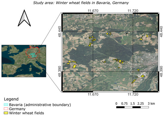
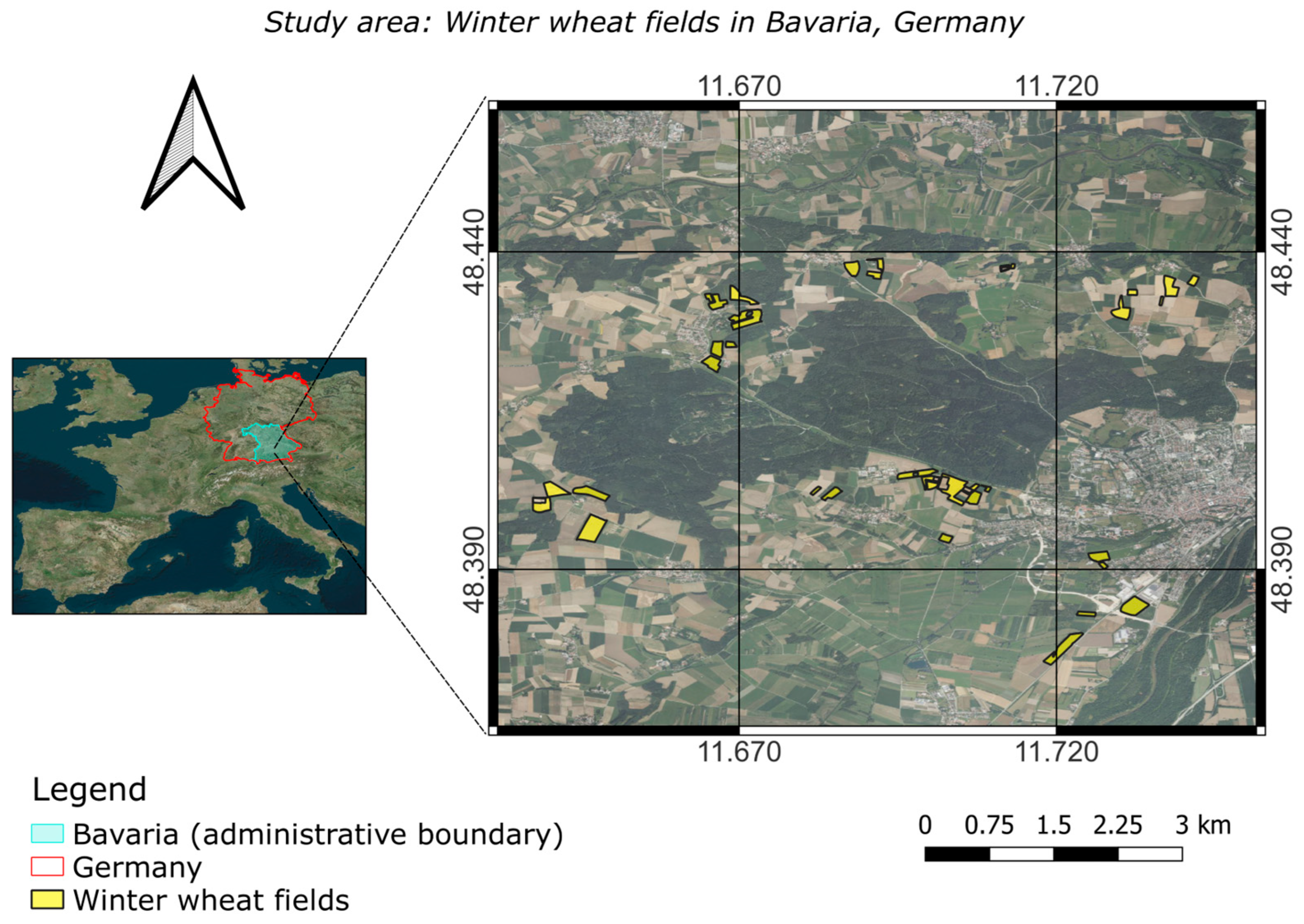
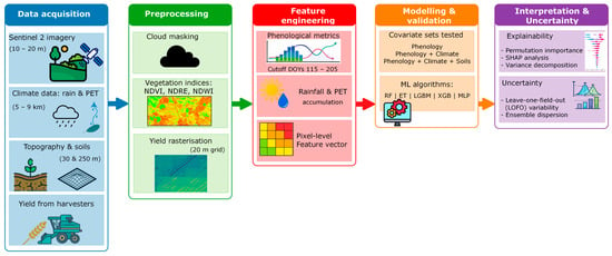
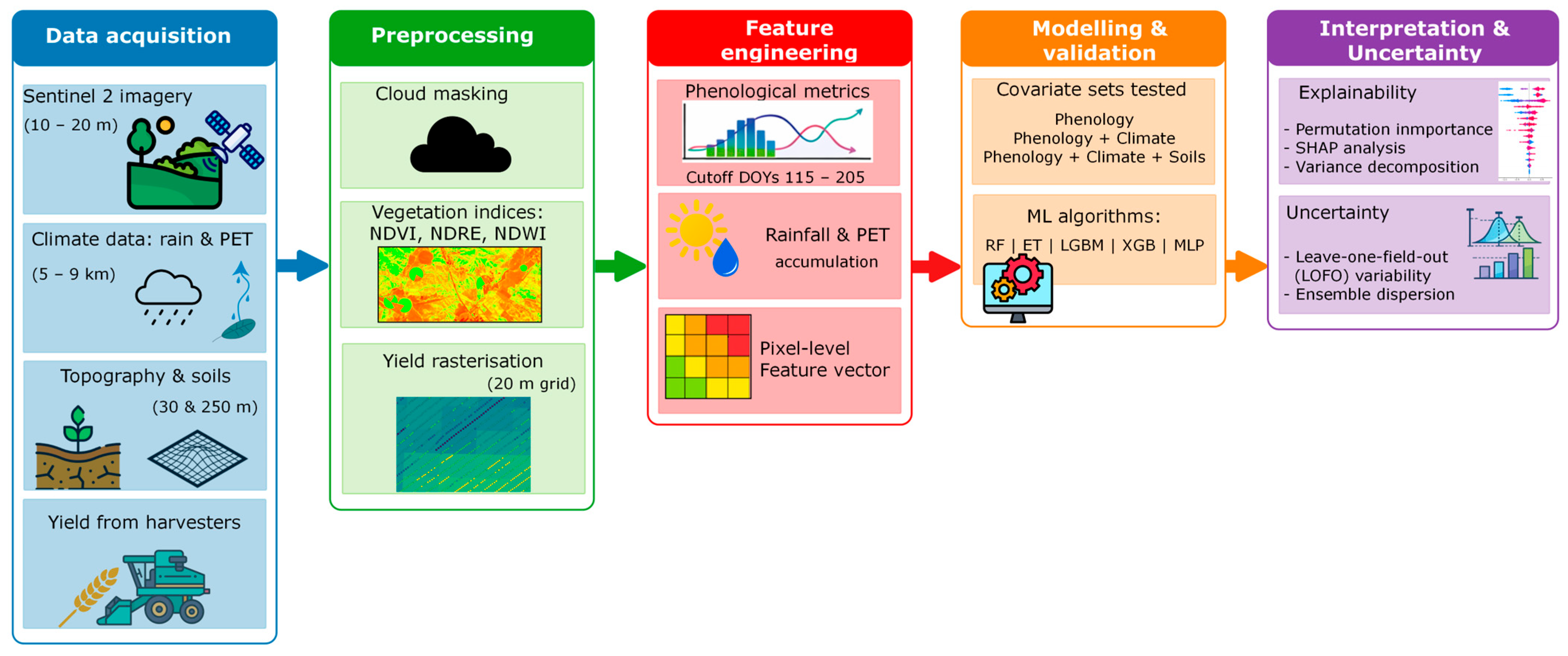
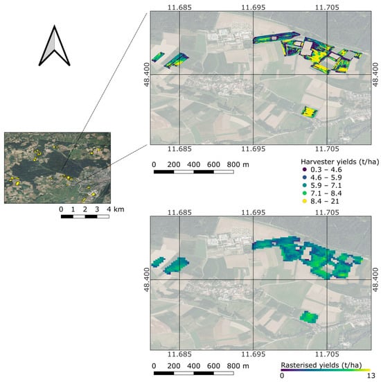
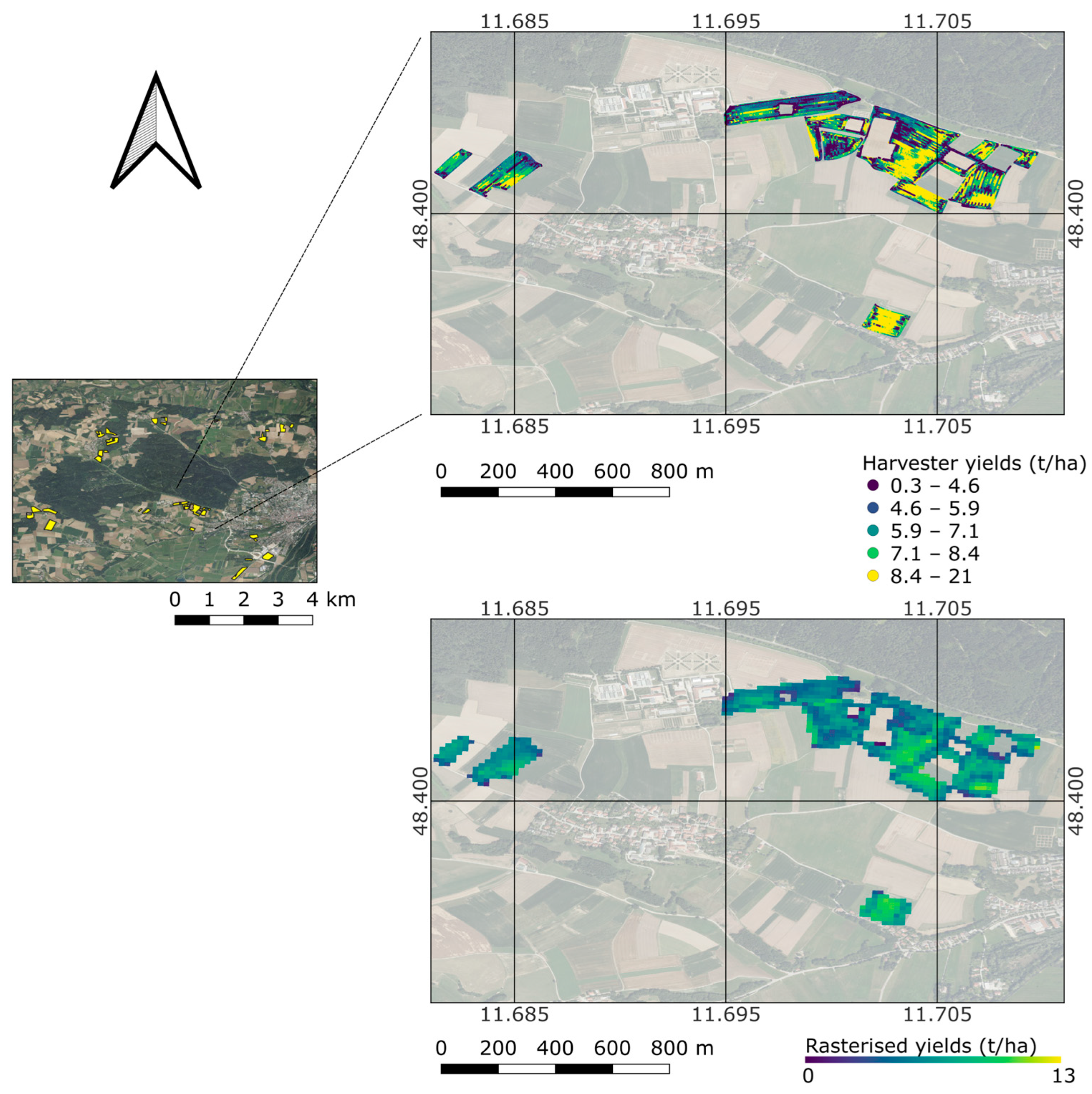
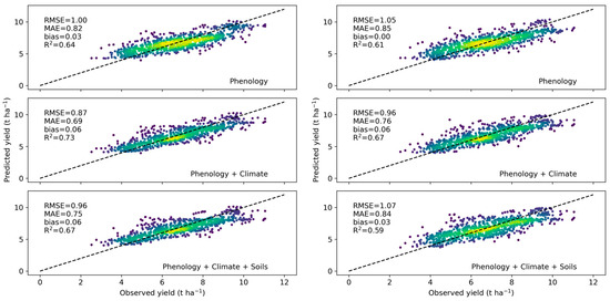
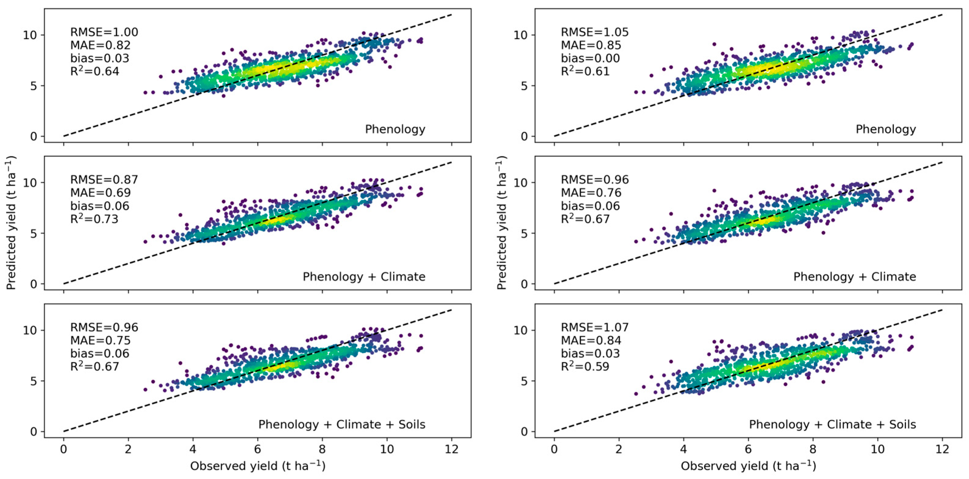
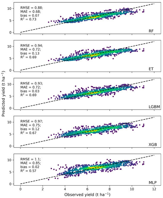
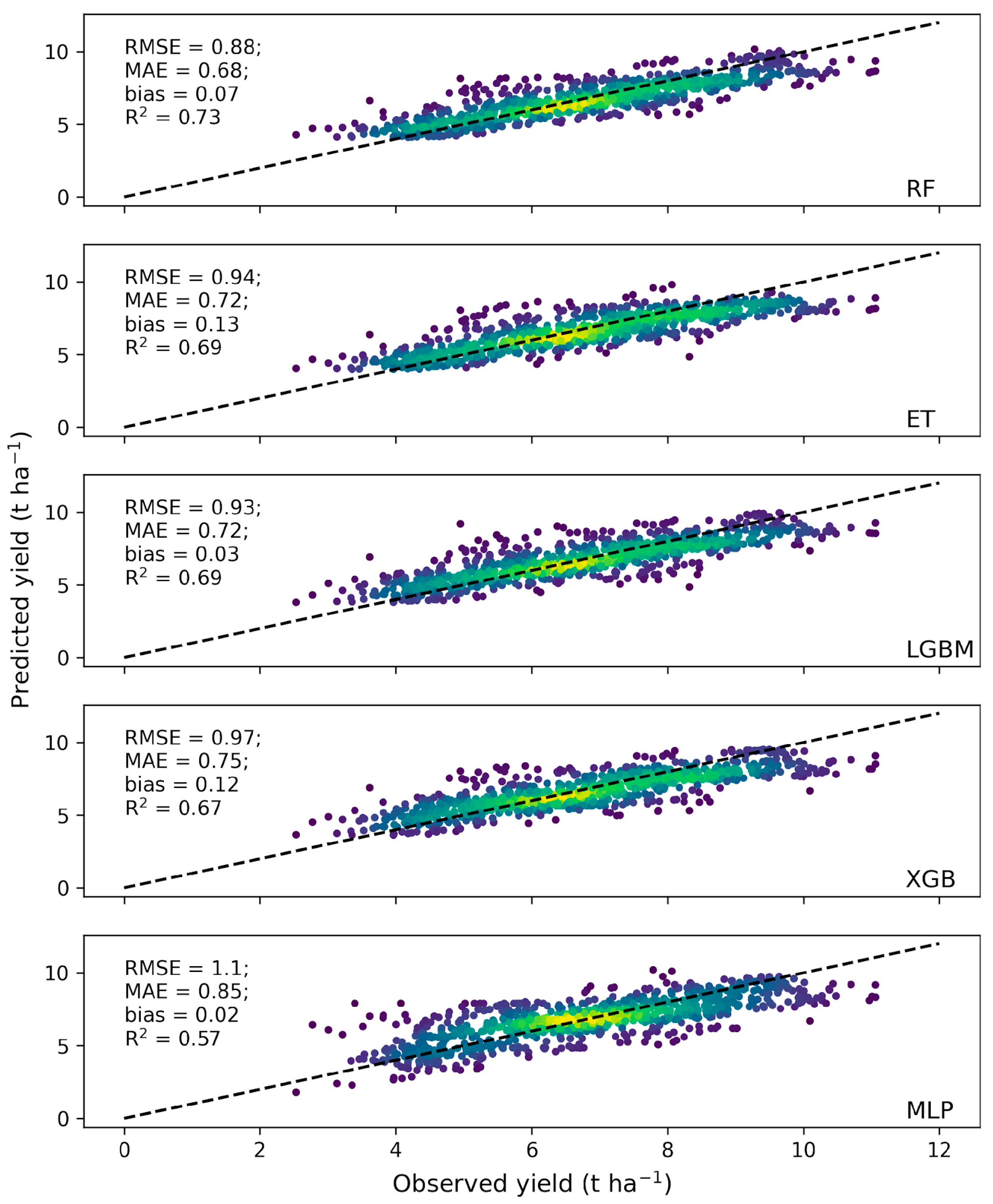
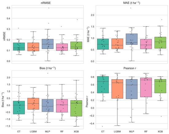
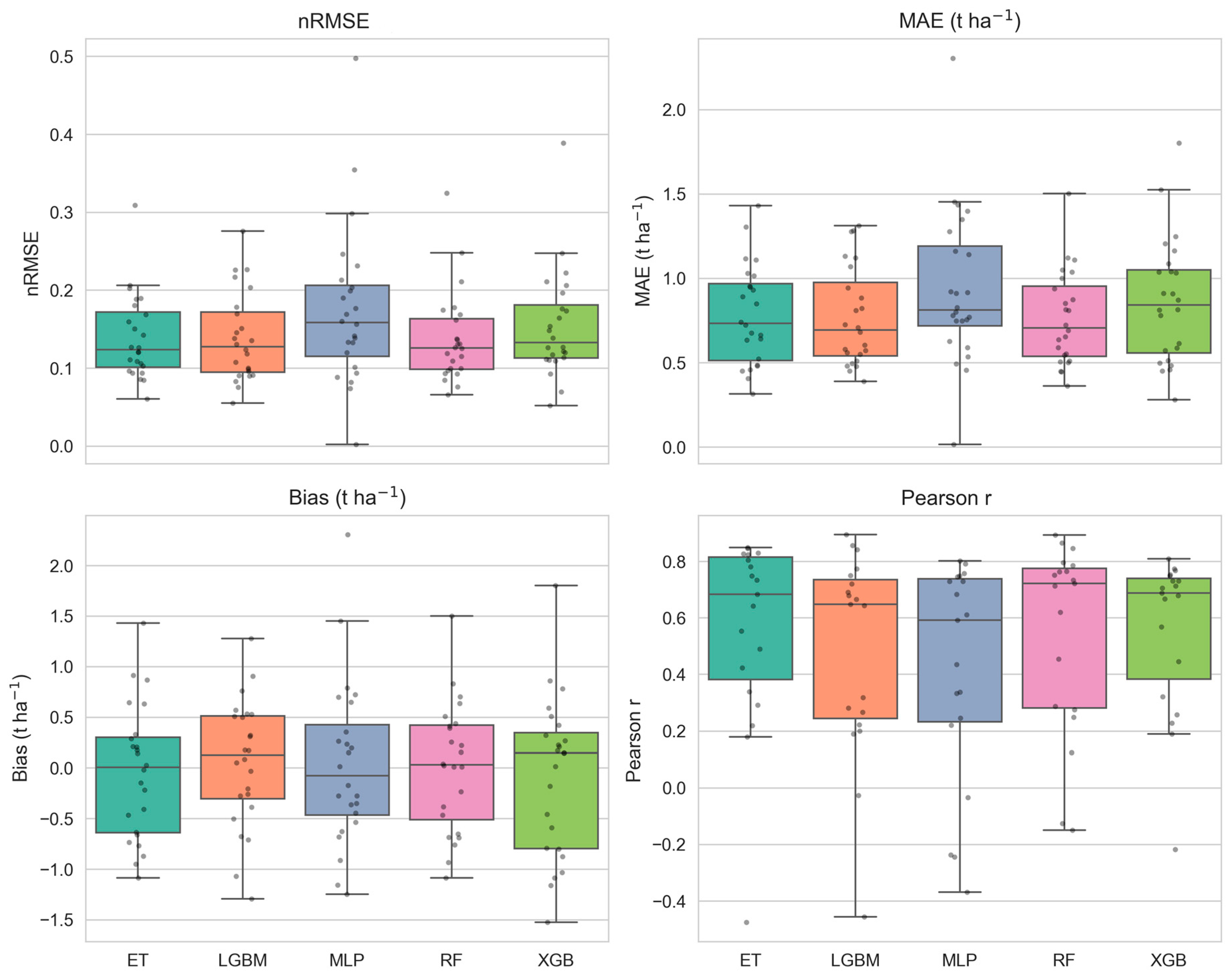
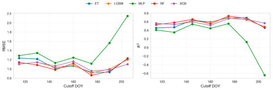
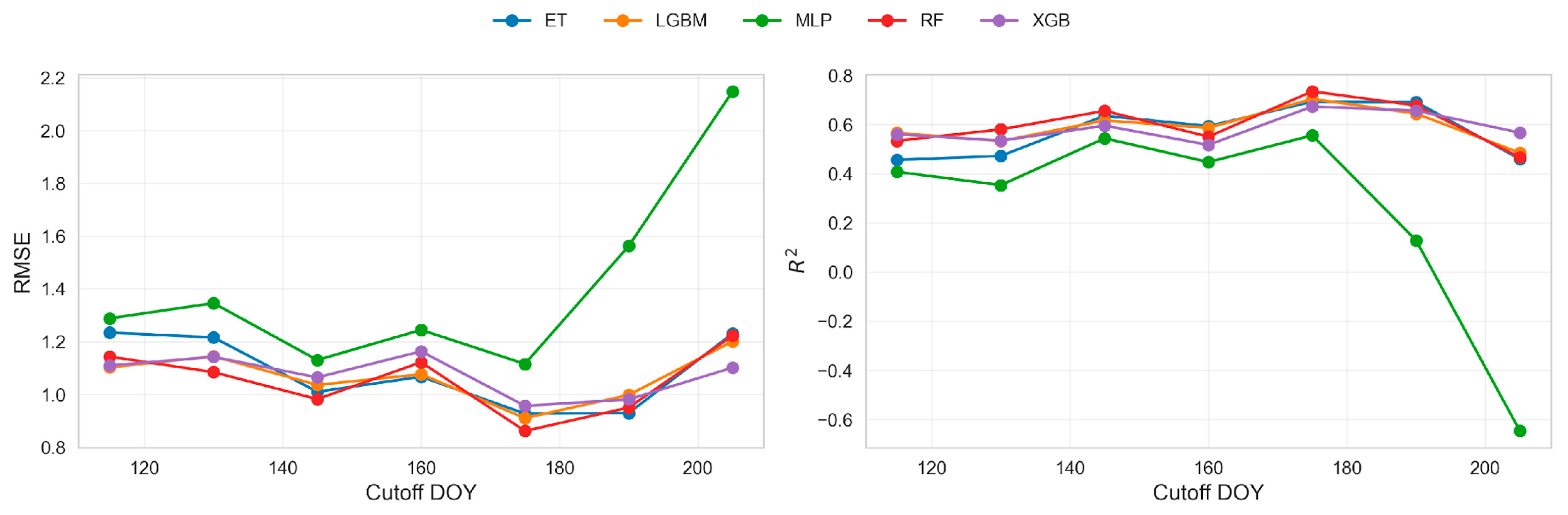
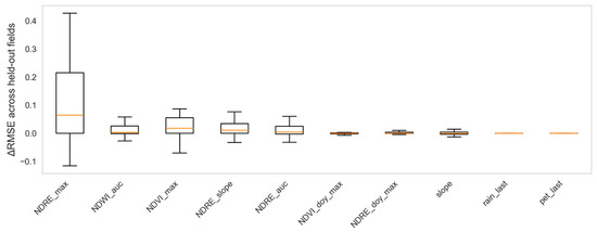
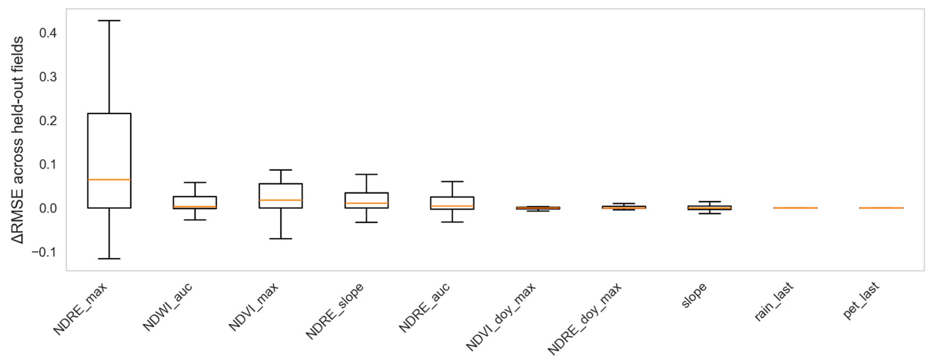
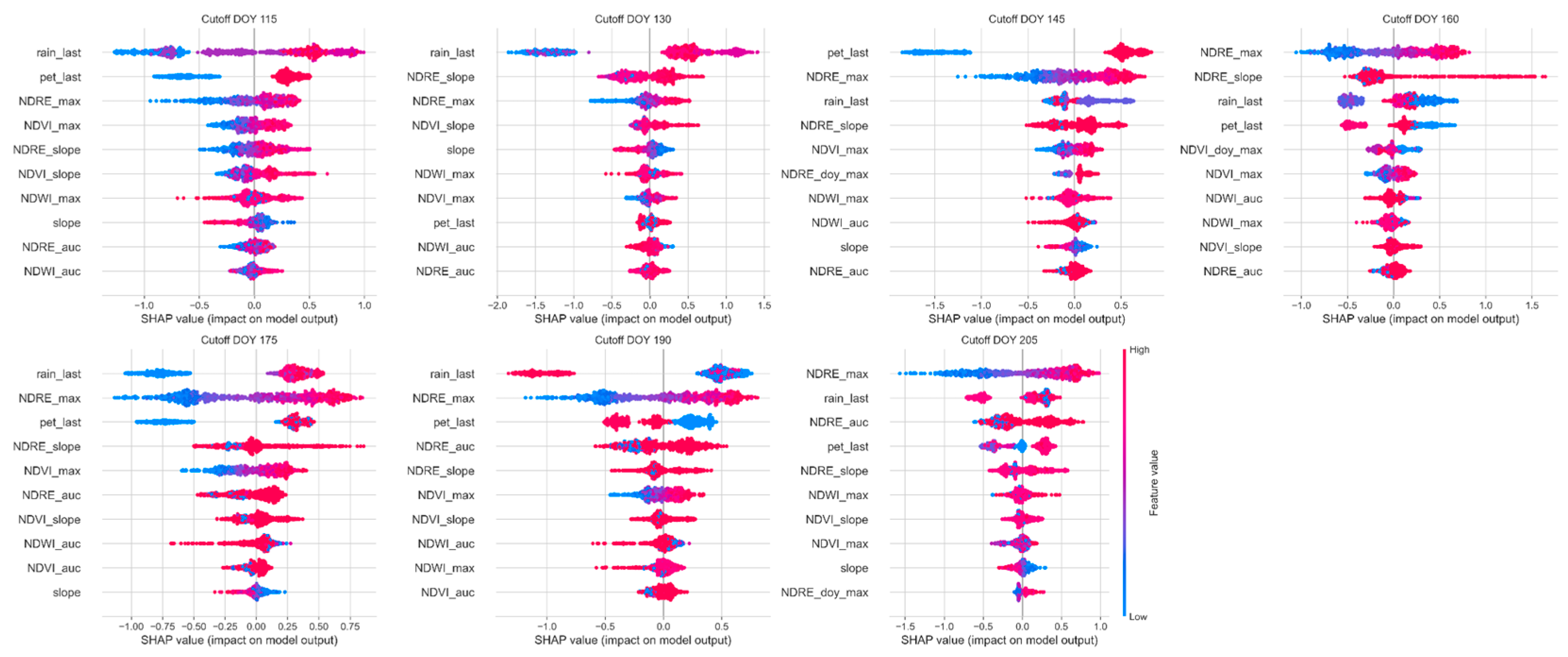
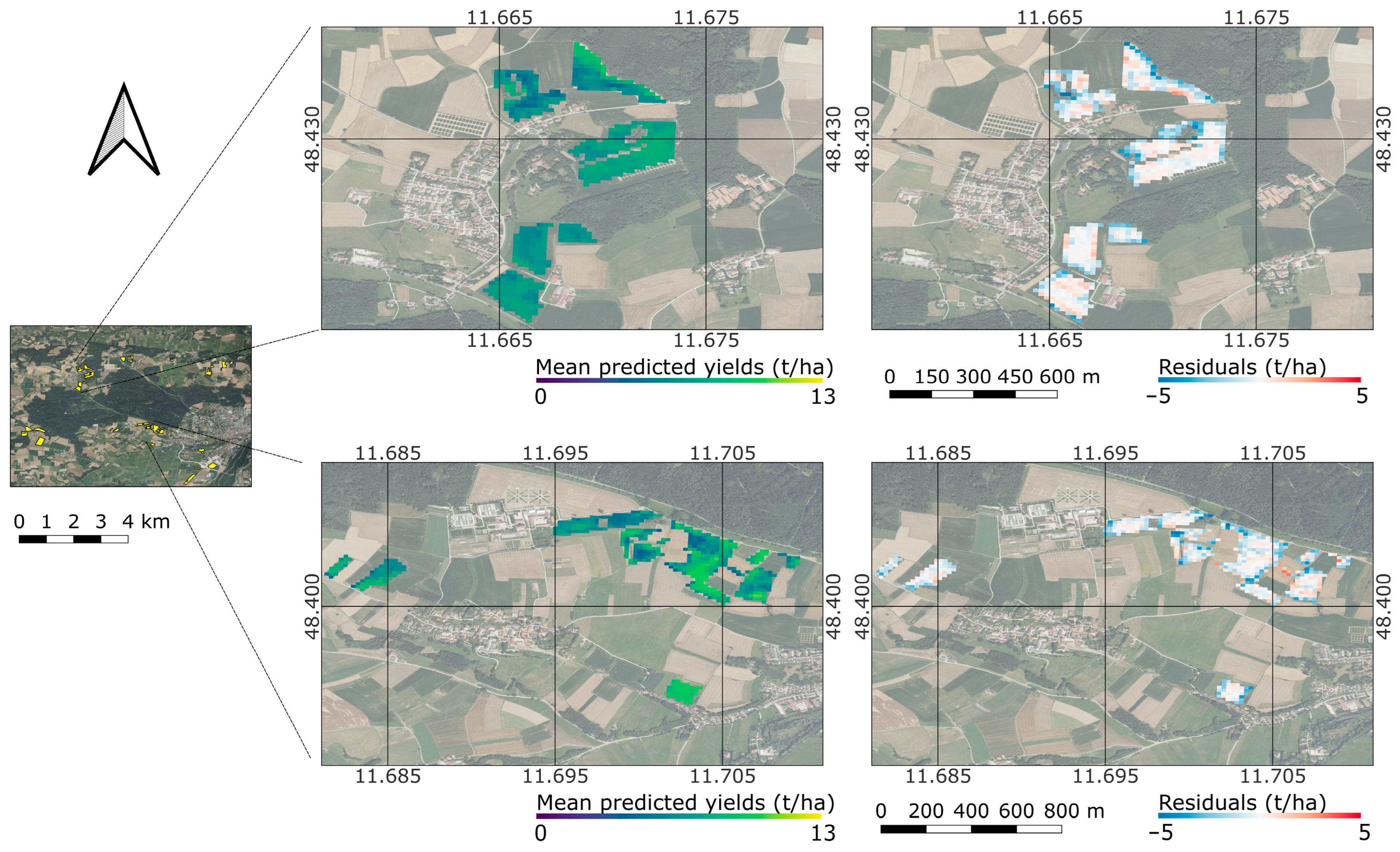
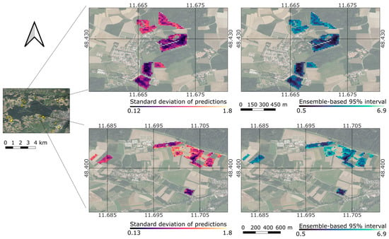
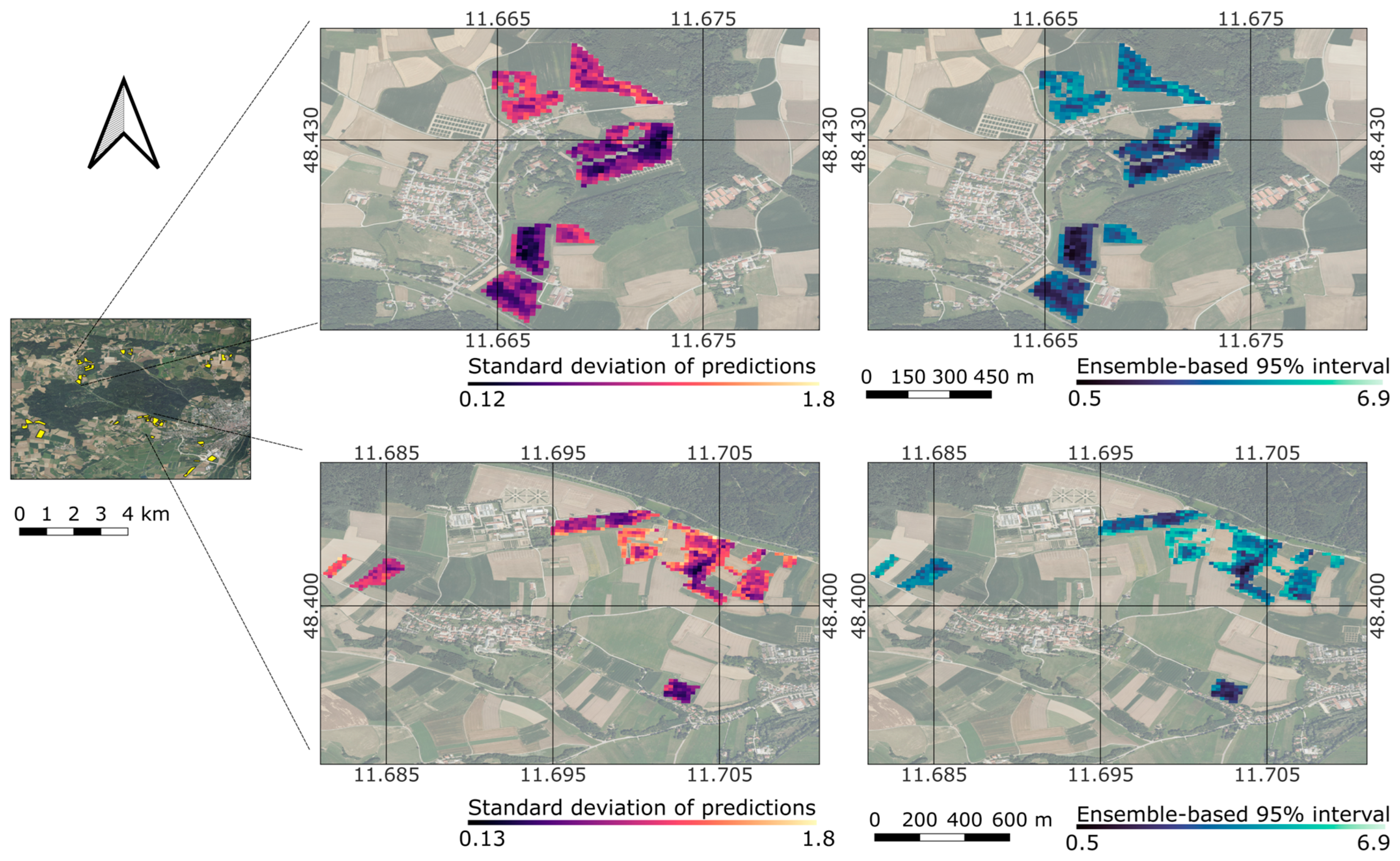

Disclaimer/Publisher’s Note: The statements, opinions and data contained in all publications are solely those of the individual author(s) and contributor(s) and not of MDPI and/or the editor(s). MDPI and/or the editor(s) disclaim responsibility for any injury to people or property resulting from any ideas, methods, instructions or products referred to in the content. |
© 2026 by the authors. Licensee MDPI, Basel, Switzerland. This article is an open access article distributed under the terms and conditions of the Creative Commons Attribution (CC BY) license.