Super-Resolution Remote Sensing Datasets for Application to Caral–Supe Archeological Sites Employing SAR and DEMs

Highlights

What are the main findings?

• A super-resolution imaging strategy for the automated investigation of archeological structure by integrating public-domain Synthetic Aperture Radar (SAR) time-series images with a Digital Elevation Model (DEM) and its deep learning algorithms.
• Its application to archeological features at the Caral–Supe ancient civilization sites.

What are the implications of the main findings?

• The technique provides a powerful way to exploit public-domain SAR data for archeology, maximizing the resolution of both electromagnetic and topographic data.
• The findings indicate that many artificial structures in Caral–Supe remain undiscovered, providing new insights into early South American civilization.

Abstract

Publicly accessible spaceborne remote sensing datasets often lack the spatial resolution required to reliably distinguish archeological features from their surrounding geomorphological contexts. In this study, we assess the potential of super-resolution (SR) products derived from multiple public-domain remote sensing datasets for a systematic archeological survey in the Caral–Supe region. We focus on Synthetic Aperture Radar (SAR) and topographic datasets—including Sentinel-1, Advanced Land Observing Satellite (ALOS) Phased Array L-band Synthetic Aperture Radar (PALSAR), and Digital Elevation Models (DEMs)—because of their capacity to detect subtle surface expressions and shallow subsurface structures obscured by vegetation or sediment cover. Using state-of-the-art deep learning algorithms, primarily employing the Enhanced Super-Resolution Generative Adversarial Network (ESRGAN) architecture, we integrated multi-source SAR imagery and DEM data to generate SR products that reveal distinct signatures in areas containing dense archeological remains and clearly delineate shallow, buried anthropogenic features. We further developed deep learning classification models that combine SR SAR and DEM inputs and trained them on known archeological site locations. This approach enabled the detection of previously undocumented structural features distributed along the coastal margin and throughout the Supe Valley. Our findings indicate that enhancing publicly available remote sensing datasets with advanced SR techniques can provide cost-effective and practical high-resolution archeological data, compared to data mining using aerial photography and high-resolution commercial satellite imagery, in terms of both cost and obstacle penetration.

1. Introduction

Archeological mapping has greatly benefited from recent advances in remote sensing technologies, both aerial and spaceborne [1,2]. The aerial platforms, in particular, have recently expanded in terms of coverage, resolution, and cost efficiency due to their adaptability [3]. Nevertheless, the value of spaceborne remote sensing remains essential. Contemporary archeological studies increasingly address large-scale spatial contexts, such as networks of ancient human settlements [4], trading routes [5], irrigation channels [6,7], and populations of mounds [8], which extend far beyond the spatial reach typically achievable through aerial surveys.

Cloud-based geospatial platforms such as Google Earth Engine (GEE), the Microsoft Planetary Computer, and various space-agency data gateways have further improved the accessibility and interpretability of satellite data. These platforms allow users, including archeologists, to acquire and analyze spaceborne imagery at no cost. However, the spatial resolution of public-domain data is often limited. Publicly available Digital Elevation Models (DEMs), including the Shuttle Radar Topography Mission (SRTM), the Advanced Spaceborne Thermal Emission and Reflection Radiometer (ASTER) Global Digital Elevation Map (GDEM), the Advanced Land Observing Satellite (ALOS) World 3D-30 m (AW3D30), and the Copernicus 30 m (COP 30) DEM, typically offer 30 m resolution. Similarly, public-domain Synthetic Aperture Radar (SAR) image products usually provide resolutions in the range of 10–25 m. These spatial scales are often insufficient for detailed archeological investigations focused on individual sites.

To overcome the resolution limitations inherent in public-domain datasets, archeological researchers have long relied on spaceborne imagery from declassified U.S. reconnaissance missions such as CORONA and HEXAGON [9], which offer sub-meter to few-meter resolutions, as well as on commercial optical and SAR imagery when resources permit. Nevertheless, public-domain datasets retain unparalleled advantages. Their global or near-global spatial coverage enables concurrent examination of archeological sites and their environmental contexts. They also provide access to three-dimensional topographic information and radar backscatter characteristics not typically available from optical imagery. Recent studies confirm that the COP 30 has successfully delineated large-scale paleoenvironmental landscapes [10] and extensive buried artificial structures [11], partly because AW3D30 and COP 30 are undersampled from higher-resolution source products that preserve finer morphological detail than their nominal resolution suggests [12]. Newly introduced DEM parameterizations have further improved detection of archeological features, while the combined use of modern SAR wavelengths conveys electromagnetic scattering information around artificial structures [13], supported by depth-dependent electromagnetic wave penetration [14,15,16]. Despite this potential, public-domain DEMs (30 m) and SAR archives (10–25 m) remain underutilized relative to costlier LiDAR and commercial imagery for archeological investigations, primarily because their spatial resolution often fails to capture features such as road networks, irrigation channels, and architectural remnants.

Our study addresses these resolution limitations by applying super-resolution (SR) algorithms to public-domain SAR and DEM datasets. SAR data are especially valuable in this context, as longer wavelengths permit partial penetration through topsoil and sparse vegetation canopy [17,18]. L-band signals, for instance, can detect subsurface features a few meters below the surface depending on soil moisture and dielectric properties. However, coarse resolution limits the ability to distinguish surface, dihedral, and volume scattering contributions from background clutter such as seasonal vegetation. Conventional single-image SR, whether classical or deep learning-based [19], tends to enhance the dominant backscatter within each resolution cell while preserving inherent noise components, such as speckle and undesired volume scattering. It is therefore insufficient for selectively enhancing weak archeological signatures. The resolution-enhancing approaches using interpolation or pan-sharpening are even more problematic, as they do not refine the actual information delivery.

Similar limitations arise when SR is applied to single-source DEM data, where interpolation artifacts and smoothing of fine-scale topographic features degrade morphological boundaries.

To solve these constraints, our approach exploits dense time-series (TS) archives from contemporary missions, such as Sentinel-1 (S-1) and ALOS Phased Array type L-band Synthetic Aperture Radar (PALSAR) 1/2, which continuously acquire data. TS SAR images are accumulated and grouped by viewing geometry (ascending/descending), polarization (VV/VH or HH/HV), and radar wavelength (C- or L-band). Through stacking and transformation, temporally incoherent components such as speckle are suppressed, while persistent backscatter signatures are reinforced. The resulting multiband composites are then processed using the Enhanced Super-Resolution Generative Adversarial Network (ESRGAN) [20], producing multi-channel SAR products with spatial resolutions of approximately 1.5–5 m compared to the original 10 m S-1 or 25 m ALOS PALSAR imagery. The improved resolution, combined with the inherent depth sensitivity of different radar wavelengths, enhances discrimination of subsurface backscatter contributions while reducing residual clutter. A complementary strategy fuses multiple public-domain DEMs into multi-channel inputs and applies SR techniques to generate an SR topographic dataset. These SR DEM products, jointly with the SR SAR images, support refined archeological and geomorphological interpretation through deep learning-based classification.

The Caral–Supe region of Peru, the focus of our case study, contains archeological sites widely distributed along the Supe Valley and coastal plain [21,22]. The enhanced coverage and resolution of the SR SAR and DEM datasets provide the basis for examining site distributions, their relationships with local geomorphology, and potential traces of paleoenvironmental conditions. However, resolutions of 1.5–5 m are not always sufficient for visually delineating the outlines of archeological structures. To address this challenge, we additionally developed a deep learning classifier that identifies electromagnetic scattering patterns arising from microscale surface textures surrounding three-dimensional archeological features. The classifier was trained using digitized reference data derived from public mapping platforms such as Google Earth, Bing Maps, and OpenStreetMap.

After all, this study was designed to develop super-resolution algorithms tailored to public-domain SAR and DEM datasets and to evaluate their applicability to archeological investigation. The results were evaluated in comparison with existing archeological records from the Caral–Supe region. The findings reveal several locations where signatures of potential human activity dating to approximately 2500–3000 BCE appear to be preserved, and their archeological implications are discussed considering the broader regional context.

2. Test Site and Datasets

2.1. Descriptions of the Caral–Supe Civilization and Its Archeological Sites

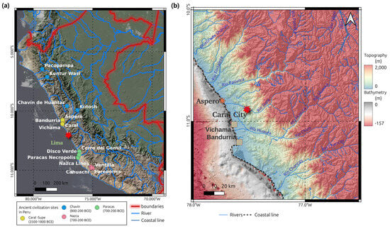
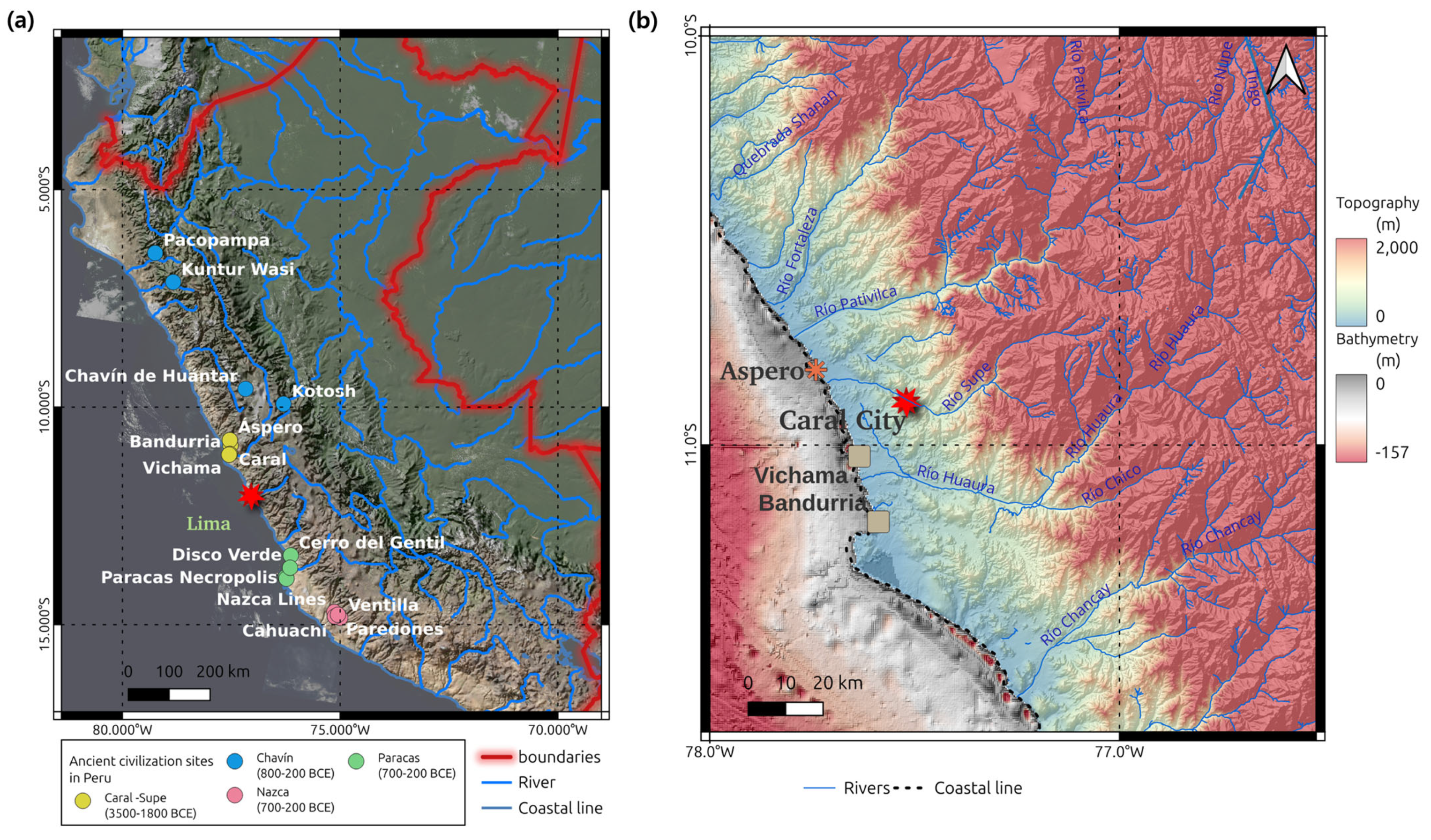
Among all ancient civilizations, the Caral–Supe civilization, located along the Peruvian coastline and within the Supe Valley, stands out as a uniquely significant case. First, it predates all other known civilizations in the New World. Second, it is remarkable for having independently developed core marks of early civilization, including complex social, economic, and religious systems, monumental architecture, and early irrigation-based agriculture. Notably, the Caral–Supe civilization reached a high level of sophistication without participation in external trade or cultural networks during humanity’s earliest stages of urban development (Figure 1a). The most striking aspect is that such an advanced form of organized labor and civic planning emerged in the third millennium BCE entirely in isolation, without technological transfer or external cultural influence. This independence distinguishes Caral–Supe from contemporaneous civilizations in the Indus Valley, Mesopotamia, and Egypt. Its footprint has reshaped modern understandings of early cultural emergence, supporting the maritime foundations hypothesis [23], which argues that abundant marine resources facilitated the rise of early civilizations along the Pacific coast of South America.

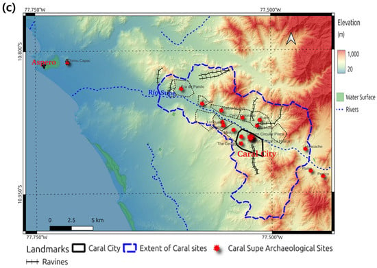
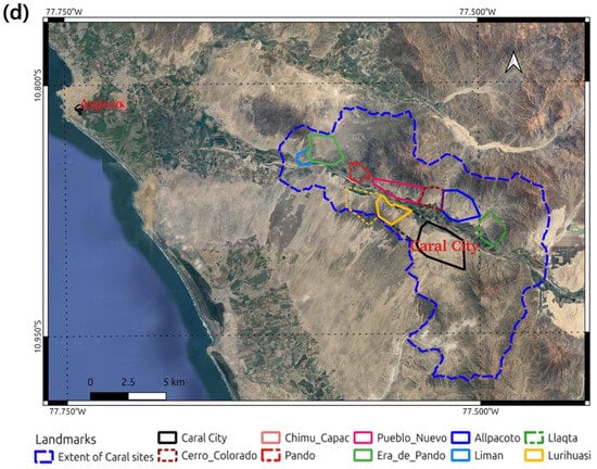
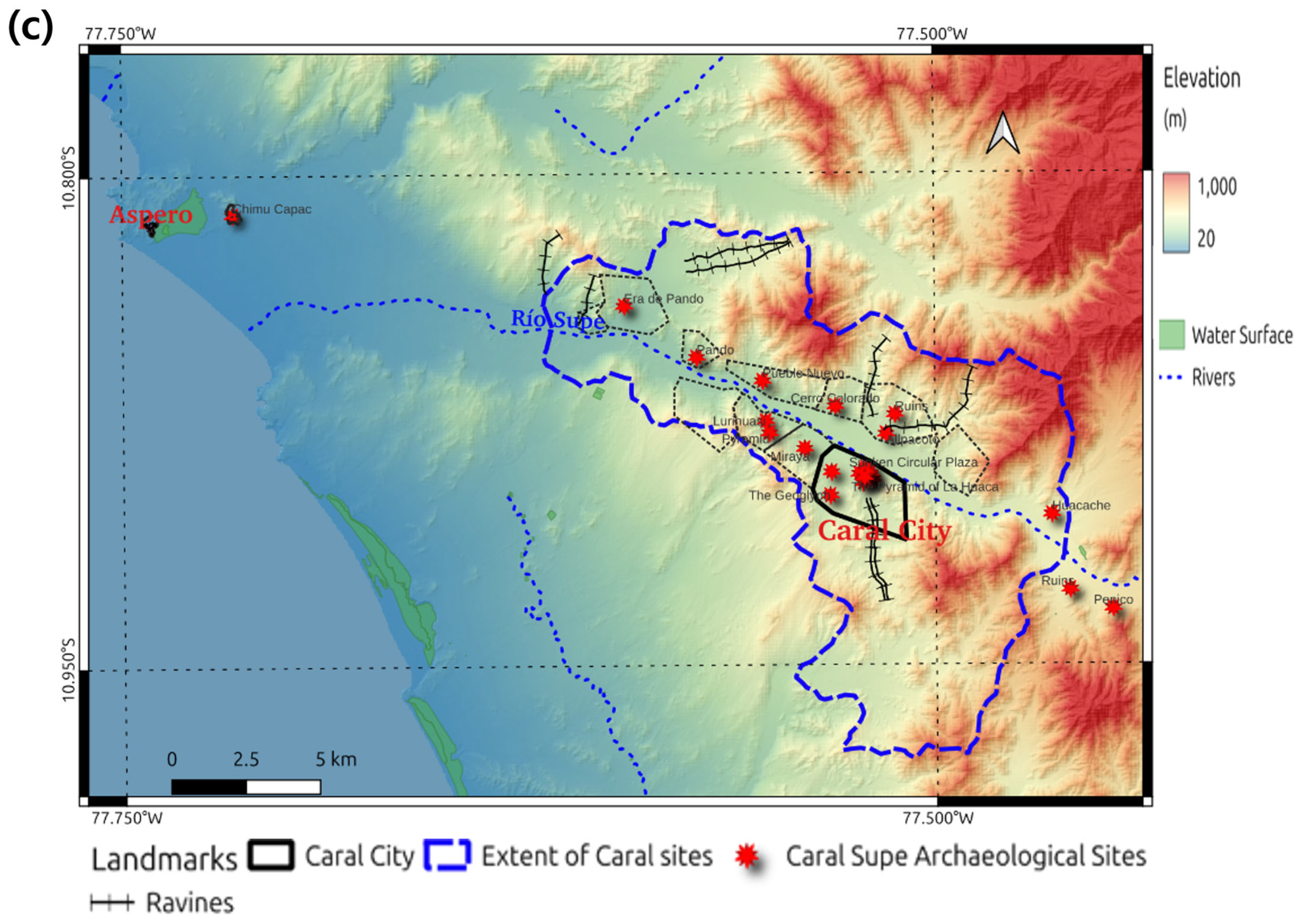
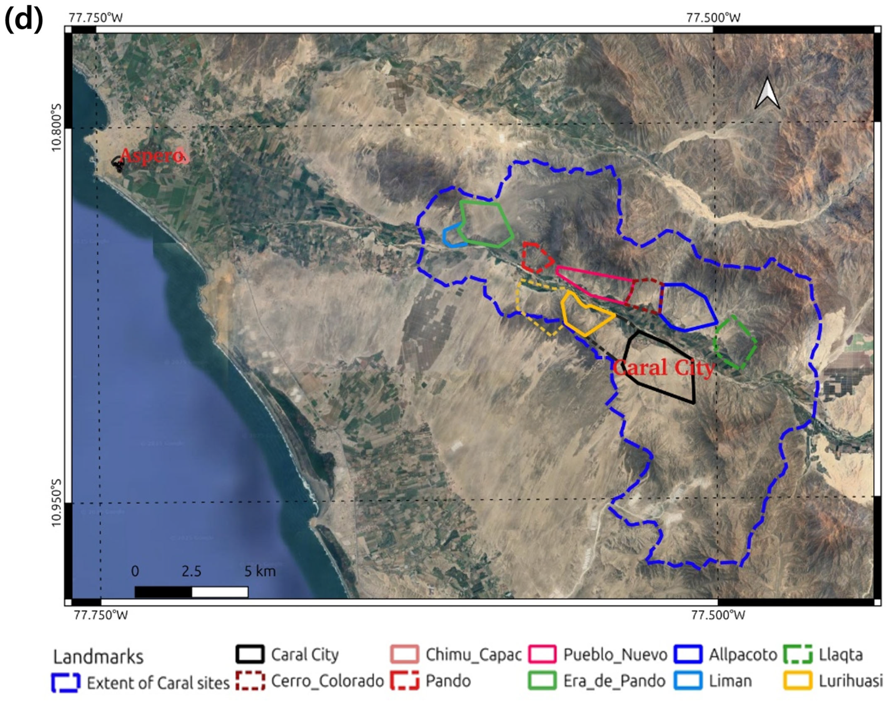
Figure 1. (a) The locations and dates of ancient Peruvian civilizations, noting that the Caral–Supe civilization predated them and acted as a mother civilization as presented in the map; (b) geographical context of the Caral–Supe civilization, showing the resource management in fishery and cultivation. Note the well-developed continental shelf along the Aspero coastal line. The populations of the Caral–Supe sites and the geomorphological backgrounds are presented using topographies, i.e., the COP 30 DEM and the global bathymetry and topography grid at 15 Arc Second (c) and a Google Satellite image (d). The sites of the Caral–Supe civilization were designated by the United Nations Educational, Scientific, and Cultural Organization (UNESCO) at https://whc.unesco.org/en/list/1269/maps/ (accessed on 5 March 2026).

Although fisheries clearly provided a crucial subsistence base, supported by the shallow, resource-rich continental shelf near Aspero (Figure 1b), as shown the recent bathymetry [24], irrigated agriculture along the Supe Valley also yielded food surpluses and cotton essential for fishing gear and textiles. These resources enabled the construction of large ceremonial centers around Caral City [25]. Assumed connections between Aspero and Caral are shown in Figure 1b,c.

Despite early investigations in 1948, the Caral–Supe civilization was not formally identified until 1997, when excavations of abandoned coastal structures revealed extensive settlements later recognized throughout the Supe Valley (Figure 1c). Radiocarbon dating places the civilization between 3500 and 1800 BCE [26]. Major sites include Aspero on the coast, interpreted as a trading hub, and the sacred city of Caral, the regional center. More recent surveys have identified numerous additional sites along the valley (Figure 1c,d), indicating diverse economic and cultural activities anchored in irrigated agriculture supported by the Río Supe and its canal systems [22]. Evidence of exchange between coastal fishing communities and inland farming populations has been recorded at Aspero, suggesting that the resulting social surplus supported the construction of monumental structures such as pyramids and amphitheaters, covering hundreds of square meters of both Caral and Aspero (Figure 1d). These edifices, built entirely by hand using shicra bags, plant-fiber containers filled with stones, were erected without mechanical tools or wheeled transport. Yet their scale is comparable to the Egyptian pyramids and major Mesopotamian Ziggujrat [22].

Within Caral, nine primary architectural complexes are distributed across the site. Each consists of a main pyramid, an open plaza, and upper-level residential units surrounded by smaller pyramids and additional monumental constructions [21,22]. The city’s population is estimated at approximately 3000 residents, with up to 20,000 inhabitants across the broader region, making it one of the densest population centers of the third millennium BCE [21]. This suggests that further residential zones may remain undiscovered. Aspero also contains monumental constructions, including a finely shaped pyramid with an estimated volume of 3000 m³ [27].

Despite these achievements, the Caral–Supe civilization exhibits several limitations often associated with its isolation from broader technological networks. It lacked pottery—critical for storage and cooking—and did not cultivate grains, relying instead on crops such as squash, beans, lúcuma, guava, and sweet potato [22]. Furthermore, no evidence of metallurgy, wheeled transport, or a strongly centralized political authority has been found. Consequently, large-scale infrastructure or administrative artifacts are unlikely to be present at Caral–Supe sites.

The contextual map of Caral–Supe settlements in Figure 1c,d provides important guidance for remote sensing-based archeological surveys. First, sites belonging to the later Chimú Capac civilization (AD 1600–1700) lie interspersed among Caral–Supe remains [28]; while useful as indicators of human construction, they must not be misidentified as Caral–Supe sites. Second, the Rio Supe and its valley clearly defined zones of habitation and cultivation, with natural levees and abandoned channels forming suitable surfaces for settlement and agriculture. Third, coastal dunes have migrated into the inland, ascending hillsides and partially encroaching into the valley. This phenomenon reflects climatic fluctuations associated with El Niño events [29], which may have contributed to the eventual dispersal of the Caral–Supe population.

2.2. Datasets

Two distinct SAR datasets were utilized in this study. The first dataset comprised C-band S-1 SAR imagery from the European Space Agency (ESA). The second dataset featured L-band PALSAR-1/2 images from the Japan Aerospace Exploration Agency (JAXA)’s ALOS platforms.

S-1 operates in Interferometric Wide Swath (IW) mode, delivering 5 × 20 m images, which serve as the primary product for this analysis. Its two polarization modes (HV and VV) [30] and two viewing geometries (ascending and descending) were employed in this research to form a multi-channel image. Leveraging S-1’s 12-day revisit interval, a total of 75 SAR images were generated to produce enough TS datasets. To mitigate potential processing inaccuracies, all data products were sourced directly from GEE in the form of Ground Range Detected (GRD) imagery, which was processed using the Sentinel-1 Toolbox (https://earth.esa.int/eogateway/tools/sentinel-1-toolbox, accessed on 5 March 2026) to generate a calibrated, ortho-corrected product (https://developers.google.com/earth-engine/datasets/catalog/COPERNICUS_S1_GRD, accessed on 5 March 2026) at 10 m resolution.

ALOS-1/2 were satellite missions launched in 2007 and 2014, respectively, for land-cover/use mapping, environmental change, and geomorphic feature tracking [31] using L-band wavelengths, which are longer wavelengths than those employed by many other SAR instruments, typically C and S bands. The L-band SAR provides better signals in environments with vegetation, soil, and snow cover. We employed Global PALSAR-1/2 mosaic products (available at https://www.eorc.jaxa.jp/ALOS/en/dataset/fnf_e.htm, accessed on 5 March 2026) [32], which are accessible via GEE. The products are 25 m resolution global mosaic of PALSAR-1/2 backscattering coefficient images in both HH and HV polarization covering the period from 2007 to 2024 at yearly intervals. The incidence angle correction and the correction over the mosaicked edge were already applied. The details of the products are given in [33].

The penetration depth of ALOS PALSAR-2 imagery is a critical factor in this study, particularly for detecting subsurface microscale scatterers and dielectric components associated with artificial structures, likely archeological targets. An earlier study provides valuable information demonstrating the potential for identifying subsurface objects [17,34]. However, penetration depth is primarily influenced by two factors: vegetation density and soil moisture [15,35,36]. In the context of Caral–Supe sites, these conditions, abundant vegetation and significant humidity, limit the effectiveness of L-band radar penetration.

The use of SR DEM alongside SAR is critical to this study, providing three-dimensional information on basements, where the most interesting SAR signals occur. The COP30 DEM (available at https://dataspace.copernicus.eu/explore-data/data-collections/copernicus-contributing-missions/collections-description/COP-DEM, accessed on 5 March 2026) is derived from the WorldDEM [37], which was produced using TanDEM-X mission Interferometric SAR (InSAR) processing [38]. The COP 30 DEM is a resampled version of the WorldDEM processed by the German Space Agency (DLR) with additional operations such as gap filling, flattened water bodies, and cut coastlines. Given WorldDEM’s 5 m grid spacing and its vertical and horizontal accuracies of 2.5 m and 6 m, respectively [39], the resulting COP30 DEM captures terrain detail more effectively than other public-domain DEMs. However, incorporating additional public-domain DEMs remains necessary, as the goal is to merge multiple datasets into higher-resolution composite products. Therefore, we employed four other public-domain DEMs, including SRTM, ALOS AW3D30, and the ASTER GDEM version 3 (v.3). All DEMs except ASTER GDEM v.3 are available on GEE, but GDEM v.3 was accessed via NASA data explorer. The input image datasets used in this study are given in Table 1.

Table 1. Characteristics of the employed datasets.

Data	PALSAR 1/2	Sentinel-1	DEM
Resolution	25 m	10 m	30 m
Covering periods	2007–2024	2020–2023	SRTM: 1999 AW3D30: 2006–2011 GDEM v3: 2000–2013 COP 30: 2010–2015
Input image number	14 images (one image per year during 2007–2010 and 2015–2024)	224 images in ascending mode 179 images in descending mode	4 DEMs
Polarizations/looking directions	HH/HV Ascending–descending mode mixed	VV/VH Ascending/descending	-
Wavelength	24 cm, L band	5.6 cm, C band	-

For deep learning validation and training datasets, we used various GIS sources, including OpenStreetMap GIS data for Peru covering buildings and roads, and digitized footprints of ancient structures extracted from Google Earth.

3. Methods

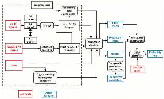
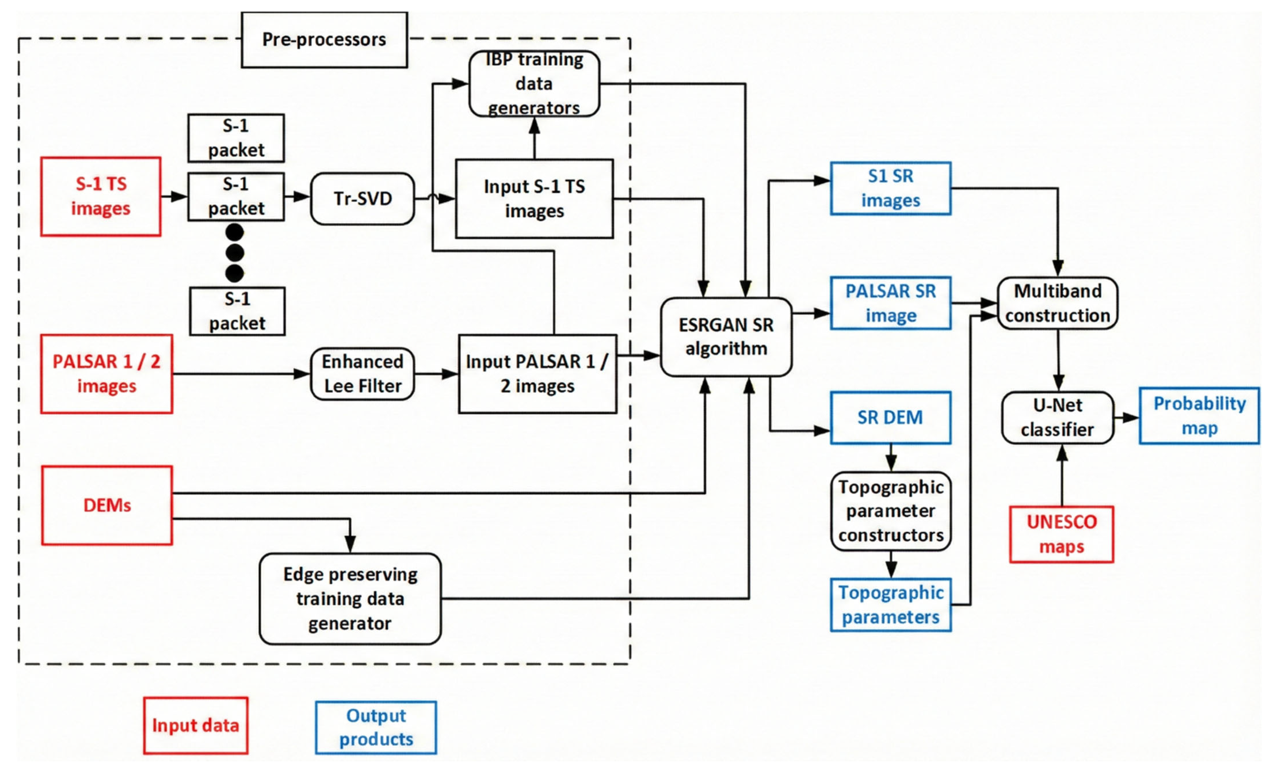
Our data processing workflow generally includes three main steps: the pre-processor, the SR processor, and the classifier, as shown in Figure 2. The following sections provide detailed information about each component.

Figure 2. Data processing flows from input image creation to probability map generation.

3.1. Pre-Processing

All topographic products are aligned with the same references, i.e., UTM WGS 84 Zone 18S, for consistency. Vertically, all four public-domain DEMs were converted to WGS 84 ellipsoidal heights using the Earth Gravitational Model (EGM) 84.

We used TS image sets of backscattering coefficients and their two polarization channels, specifically the HH and HV channels from ALOS PALSAR-1/2. The pixel values in these data files were converted to backscattering coefficients using the following:

σ⁰ = 10 log₁₀(PV²) + control_factor

(1)

where σ⁰ is the backscattering coefficient, PV is the pixel value of the data file, and control_factor is the calibration coefficient (−83.0) [32]. In addition, we employed the enhanced Lee filter [40] to suppress speckles of ALOS PALSAR images. It is worth noting that [16,17,18] estimated the penetration depth of the L-band SAR image as 1.5 to a few meters in a dried desert environment. However, based on our experience, the penetration depth of ALOS PALSAR-2 is much shallower, but it can observe shallow surface objects.

For the S-1 TS dataset, we used VV and VH polarization images in both ascending and descending acquisition modes. A key challenge in pre-processing S-1 TS data is ensuring signal consistency. Because the TS images were acquired with nearly identical viewing geometries, i.e., similar heading and incidence angles within the same frame and track, variations within a given mode primarily reflect changes in surface conditions, such as vegetation dynamics, soil moisture fluctuations, or human activities.

Our objective, however, is not to track these temporal variations, but to isolate the weak and stable signals associated with concealed archeological features. This requires applying algorithms that suppress time-variable surface effects, as well as conventional SAR noise and speckle, while preserving the subtle, consistent backscatter signatures of interest.

For this purpose, we designed a packet-based transform as proposed in [41]. We reorganized the full S-1 TS SAR images into multiple packets, each containing three temporally adjacent images with identical polarization and acquisition direction. Each packet therefore spans approximately 1–1.5 months. Within each packet, we applied dimensionality-reduction techniques, which means image transformations designed to suppress short-term temporal fluctuations and other SAR noise. After testing several image-rotation and decomposition methods, we selected truncated singular value decomposition (tr-SVD), as it effectively isolates stable, independent components while filtering out temporally inconsistent signals [42]. Tr-SVD is quite similar to principal component analysis but is more effective at eradicating temporal components. Thus, tr-SVD aligns well with our goal of retaining both the dominant backscatter signal from surface structures and the weak, stable components associated with shallow subsurface features. Applying tr-SVD across the full time series allowed us to compress 75 S-1 images into 25 first-order tr-SVD packets. This transformation enhances consistent signals from specific land-cover types, such as rocky surfaces, built-up areas, and bare terrain, and provides inputs that are well suited for deep learning-based resolution enhancement. For PALSAR 1/2, the number of time-domain images is insufficient to generate tr-SVD-based input image sequences. Therefore, we applied an enhanced Lee filter to each yearly PALSAR image and generated 14 filtered input images spanning 2007 to 2010 and 2015 to 2024.

3.2. Super Resolution

In this study, SR was defined as a line of algorithmic approaches to enhance the resolution of raster datasets. It was first applied to medical images and astronomical datasets [43,44], then extended to photo images using mobile sensors, and introduced into remote sensing [45]. A few standards can classify the approaches of super resolution: (1) single vs. multiple images, which make enhanced resolution of the output image from a single image or multiple images (likely multi-temporal images); (2) supervised vs. unsupervised images, which depend on the availability of training datasets, as explained by [46]. Considering our study case, in which multi-temporal images arise from consecutive SAR acquisitions and a lack of high-resolution training images, it is natural to employ multiple temporal and unsupervised super-resolution algorithms. However, it became clear that newly introduced deep learning-based supervised approaches, such as Convolutional Neural Network (CNN) and Generative Adversarial Network (GAN)-based methods, are superior to conventional unsupervised super-resolution algorithms, such as Iterative Back-Projection (IBP) [47] and Projections onto Convex Sets (POCS) [48]. Thus, we introduced a hybrid approach that produces a high-resolution training image using an unsupervised method and uses it as a training dataset for the supervised method. It should be noted that the SR of SAR imagery is a complex problem, although it has been addressed in a few studies, especially with public-domain SAR imagery. Our case is quite peculiar, as our objective is to construct SR SAR images from multiple TS SAR datasets acquired under the same imaging conditions but at different times. For a deep learning-based approach, there are two commonly applied deep learning structures: (1) Super-Resolution Generative Adversarial Networks (SRGANs) [49]; (2) Enhanced Super-Resolution Generative Adversarial Networks (ESRGANs) [19,20]. At first, SRGAN did not show better performance than the unsupervised training data. Therefore, we concentrated on ESRGAN. Inputs to the two super-resolution schemes are TS SAR images generated from tr-SVD of S-1 and enhanced Lee-filtered PALSAR 1/2 images. The IBP algorithms generate training data for high-resolution SAR images. It is particularly important to process TS SAR images using t-SVD and the enhanced Lee filter. Without pre-filtering the input TS SAR image, the SR algorithm amplifies noise as well as the signals of interest in all input image channels in the spatial domain, resulting in a noisy SR image. The basic mechanism for GAN-based super-resolution (SR) to achieve low-to-high resolution is direct adversarial competition between two networks. The Generator creates the high-resolution image (low-to-high image synthesis), while the Discriminator, acting as a critic, provides a dynamic, learned error signal, i.e., Adversarial Loss Function, to train the Generator by judging if the generated image is fake or real. In models like ESRGAN, the Generator uses an advanced design, the Residual-in-Residual Dense Block (RRDB) [20], to make this synthesis more effective.

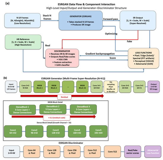
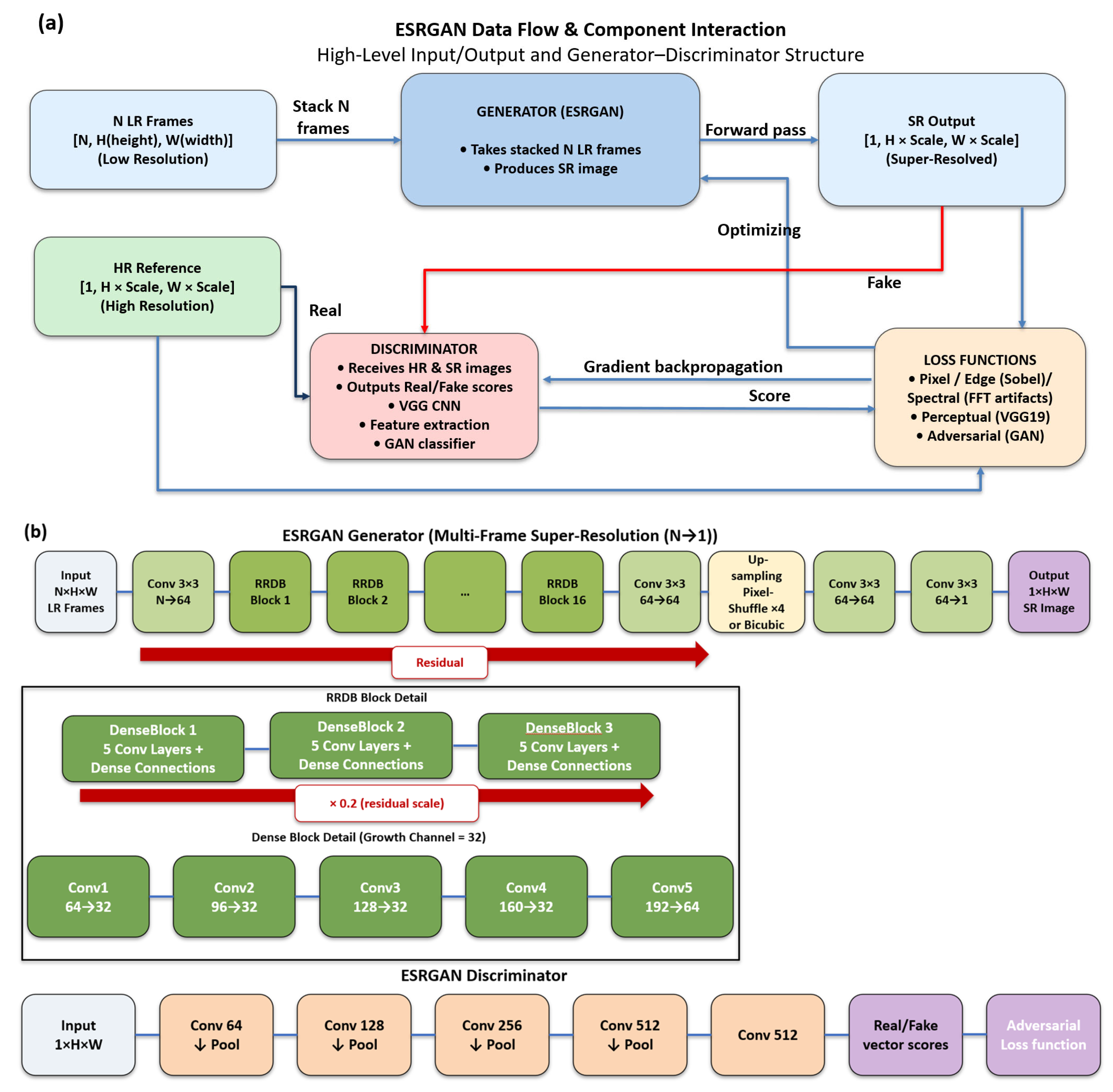
Figure 3a presents a training framework for ESRGAN tailored for multi-frame super-resolution using an N-to-1 approach, wherein N low-resolution (LR) frames are stacked as input channels to predict a single high-resolution output. The Generator architecture is based on RRDB, featuring dense blocks and flexible upsampling methods. At the same time, the Discriminator employs a Visual Geometry Group (VGG) [50]-style Patch Discriminator, which is a type of Discriminator used in GAN that classifies patches of the input image as real or fake [51]. Training proceeds in two stages, i.e., pretraining with pixel-wise losses (L1 (Mean Absolute Error), edge, spectral) to stabilize the Generator and GAN fine-tuning with adversarial and perceptual losses. The framework calculates a complex composite loss function for the Generator by combining several components: L1 loss for precise pixel-wise reconstruction, edge loss (via Sobel filter) for sharp edge preservation, and spectral regularization to minimize unrealistic high-frequency artifacts. It also includes the crucial perceptual loss based on VGG-19 feature matching, which has 16 convolutional layers and three fully connected layers within the network [50], alongside the adversarial loss using Binary Cross-Entropy (BCE) derived from the Discriminator’s critique. For stable training, the process employs random patch extraction and data augmentation, global normalization of data, gradient clipping to manage instability, and model checkpointing determined by the Generator’s performance.

Figure 3. (a) Processing flow of the ESRGAN SR processor. (b) Structure of ESRGAN SR components.

In S/W structures, the dataset loader ingests N low-resolution frames and a single high-resolution reference, stacking LR frames into a multi-channel input. Randomly aligned patches are extracted during training, and all data are normalized to [0, 1] using global statistics. These statistics (min and max) are robustly computed using the 0.5% and 99.5% percentiles of all pixel values to mitigate the impact of outliers. Each RRDB comprised three dense blocks, each containing five convolutional layers, as shown in Figure 3b. Upsampling is achieved via pixel shuffle for power-of-two scales (2×, 4×, 8×, 16×), which incorporates Initialized to Convolution NN Resize (ICNR) [52] to reduce checkerboard artifacts. The ESRGAN reconstructor is the inference/reconstruction script that uses a trained ESRGAN model to upscale images. The workflow of the reconstructor (1) loads the trained model—automatically detects architecture parameters from the checkpoint weights; (2) reads N low-resolution frames from a list and stacks them as multi-channel input; (3) performs tiled inference due to memory issues of the Graphics Processing Unit (GPU), with overlapping patches, using Gaussian-weighted blending to avoid seam artifacts; (4) saves the super-resolved output as a GeoTIFF with proper georeferencing.

In the case of SR DEM creation, the algorithm is almost identical to the ESRGAN SR algorithm of SAR. Up to now, SR DEMs have usually been created from high-resolution training data from LiDAR and UAV photogrammetry, as stated in [53]. Recent trends in SR DEM include CNN- and GAN-based algorithms [54,55], which are replacing conventional geostatistical methods, interpolation, and image analysis [56,57]. Our approach is to apply edge-preserving resolution enhancement [58] to original DEMs as ESRGAN training data. Therefore, we apply modified edge-based SR algorithms, assigning the COP 30 DEM edge, which provides overall delineation around topographic structures, 50% more weight, and a 5 m resolution training dataset. To prevent overfitting, we train on 30% of the total target area covering all elevation ranges using the ESRGAN scheme. All DEMs are carefully normalized to prevent changes in the SR DEM’s height range. The quality of such aspects will be evaluated in the next section. The potential to extract the Multi-Scale Relief Model (MSRM) [10] and Local Relief Model (LRM) [59] as well as roughness as traditional topographic parameters from SR DEM was noticed. An LRM is a parameter for a high-pass filter that removes large-scale terrain features, leaving only small-scale local variations as follows:

$$K_{\sigma }\left(i,j\right)={\displaystyle \frac{1}{2\pi {\sigma }^2}}{e}^{-\frac{i^2+j^2}{2{\sigma }^2}}$$

$$C_{Broad}\left(i,j\right)=E(i,j)\ast K_{\sigma }\left(i,j\right)$$

$$LRM\left(i,j\right)=E\left(i,j\right)-C_{Broad}\left(i,j\right)$$

(2)

where E(i,j) is a matrix of absolute elevation values, K_σ(i,j) is a Gaussian low-pass filter kernel, σ is the standard deviation, and C_Broad is the Broad-Scale Relief Component. Then LRM(i,j) can be considered a fine-scale component. The actual MSRM, which functions as a band-pass filter in terrain that retains only specific ranges of topographic frequencies, is calculated by summing and averaging the differences between low-pass-filtered surfaces at different scales, as follows:

$$MSRM={\sum }_{k=k_{min}}^{k_{max}}{w}_k(E\left(i,j\right)-(E\ast K_{{\sigma }_k})(i,j))$$

(3)

where $K_{{\sigma }_k}$ is a Gaussian low-pass filter kernel at scale k, $E\ast K_{{\sigma }_k}$, which is another expression of Broad-Scale Relief, C_Broad, at scale k, is a 2D convolution of the elevation matrix E with kernel $K_{{\sigma }_k}$, which yields the smoothed background elevation at scale k, and w_k is the weight assigned to each scale k and equal to 1/n, where n is the total number of relief models calculated; thus, an equal weighting approach is employed in this study.

3.3. Image Composition and Deep-Learning Classifications

As stated, we created multiple SR images using SAR polarization modes and viewing directions together with the SR topographic parameters. We put them into multiple channels to improve visual interpretation using the RGB color scheme, where each color band was derived from the polarization/direction of SR SAR and the topographic properties of SR DEM. Upon them, we constructed multiband SAR/DEM fused datasets for a deep learning classifier. Each of the SR SAR modes and driven topographic datasets from the SR DEM, such as roughness, LRM, and MSRM, is combined as input data for the deep learning classification. We also created training datasets from digitized archeological structure footprints from the UNESCO Caral–Supe map and Google Earth. Note that some parts of the archeological structures, such as the Penico area, are retained as validation datasets. We also constructed a negative mask map consisting of (1) a contemporary building and road footprints where archeological structures are likely concealed; (2) high sloped topography (>45 degrees) and high-altitude areas (>500 m) in which ancient residences were practically impossible; (3) water field, modern orchard, and highly developed contemporary cultivations where the furrows and boundaries are often false signatures with archeological structures. Therefore, the data flow for deep learning classification first trains a classifier on a subset of the archeological building footprints and then screens the outcomes using a negative mask map.

The problem of identifying half-damaged/buried ancient buildings’ footprints from multi-channel SAR and topographic data, given a set of known positives and a complementary negative constraint mask map, is fundamentally a challenge in the area of positive-unlabeled (PU) learning [60], which is a type of semi-supervised learning and similar to the semantic segmentation of damaged buildings [61]. The optimal strategy employs an Attention U-Net architecture to generate a pixel-wise probability map, as shown in [62,63]. The network uses a custom backbone with four downsampling and four upsampling blocks and incorporates the Attention U-Net to enhance feature fusion. The final output is an array of logits, which are unscaled numerical scores. The crucial step of converting digits into probabilities is retained until the model is used to make predictions and handled by the Sigmoid activation function.

This model is trained using a specialized approach that leverages three distinct datasets: positive data defined from an archeological building mask (P), negative data defined from mask data (Ndef), and unlabeled areas (U). To handle uncertainty and severe class imbalance, the training minimizes a custom loss function that is a weighted combination of Focal Loss, which is a special kind of loss function designed to solve the problem of extreme class imbalance by making the model focus more on hard-to-classify examples [64], and Dice Loss, a statistic used to gauge the similarity of two sets [65]; thus, the total loss is Focal Loss plus half of Dice Loss. A variation in BCE was initially applied only to the positive and negative sets, i.e., P ∪ Ndef [64]. Crucially, the approach incorporates Hard Negative Mining (HNM) [66], in which the model iteratively predicts on U to identify high-confidence false positives. A pixel is classified as a hard negative if the prediction exceeds the threshold and it is in the U area. The selection threshold for defining a hard negative is not fixed; it decreases over the training schedule to gradually incorporate more uncertainty. This HNM step enhances the model’s discriminative ability, forcing it to generalize the subtle features that distinguish true damage signatures from complex environmental or structural false alarms, thereby improving the accuracy and calibration of the final probability output [67].

4. Results

Two kinds of SR SAR composite products were generated from multi-channel datasets. S-1 TS images in four channels, i.e., ascending VV, ascending VH, descending VV, and descending VH, were produced, and selected combinations were feedforwarded as inputs to the ESRGAN model. For PALSAR-1/2, we organized the TS data into four channels based on acquisition period and polarization: HH and HV images from 2007 to 2010 by PALSAR-1, referred to as the 2010s HH and HV channels, and HH and HV images from 2015 to 2024 by PALSAR-2, referred to as the 2020s HH and HV channels. For each channel, we tested the maximum feasible SR scale and selected a target resolution of 1.5 m (UTM WGS 84 Zone 18S) for S-1 and 5 m for the PALSAR datasets.

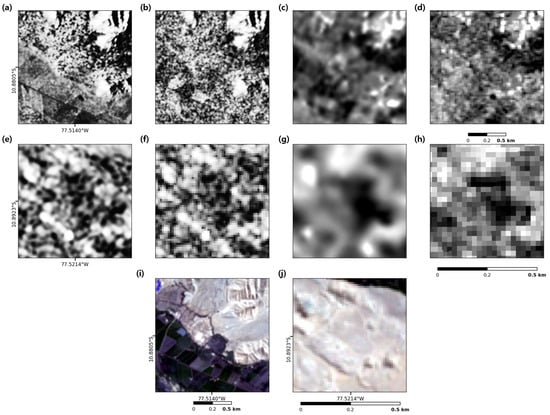
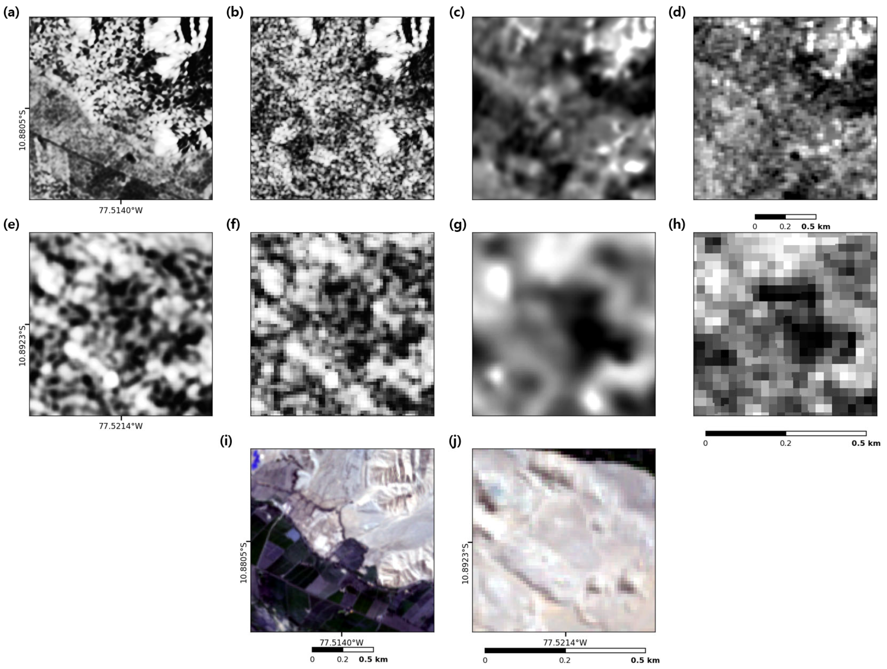
The resulting SR SAR images and SR DEM products, i.e., MSRM, LRM, and roughness, for the sectors of Caral City are shown in Figure 4. The S-1 SR image provides the clearest visual expression of near-surface and surface anthropogenic structures (Figure 4a,e). By contrast, the PALSAR-1/2 SR SAR products (Figure 4c,g) highlight their ability to detect shallow subsurface features. Since some of these improvements are difficult to discern at the display scale, the next section evaluates them quantitatively using image quality metrics.

Figure 4. (a) SR S-1 image, (b) original S-1 images, (c) SR PALSAR image, (d) original PALSAR image over Allpacoto site. (e) SR S-1 image, (f) original S-1 images, (g) SR PALSAR image, (h) original PALSAR image in central Caral City. Their corresponding Sentinel-2 optical images are in (i,j).

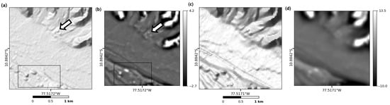
A six-times-enhanced SR DEM with 5 m resolution derived from the original COP 30 and three other DEMs is displayed in Figure 5a as hill-shaded models using identical illumination parameters (45° inclination, 270° azimuth) of the original COP 30 DEM (Figure 5c). The effects of SR processing are evident: outlines of auxiliary archeological features, such as the eastern pyramid footprints, become visible, and the major monumental structures in Caral are rendered with greater clarity in SR products. Within this context, MSRMs derived from the SR DEM and the original COP 30 DEM show substantial differences (Figure 5b,d). Notably, both have well-preserved structures within Caral (boxed region), but partially buried features at Allpacoto (arrows in Figure 5a,b) are faint or indistinguishable in the MSRM of the original COP 30 DEM.

Figure 5. (a) SR DEM in Caral City in comparison to original DEM in (d). (b) MSRM in Caral City from SR DEM in comparison to MSRM of original COP 30 DEM in (c). Note the boxed area that encircles Caral City and the arrow to the archeological structures in Allpacoto, which is on the opposite side of Caral City.

It should be noted that the SR image resolution was determined by assuming a range of 5–7 times finer as the best and then finalized by producing and visually evaluating SR sample images at those resolutions.

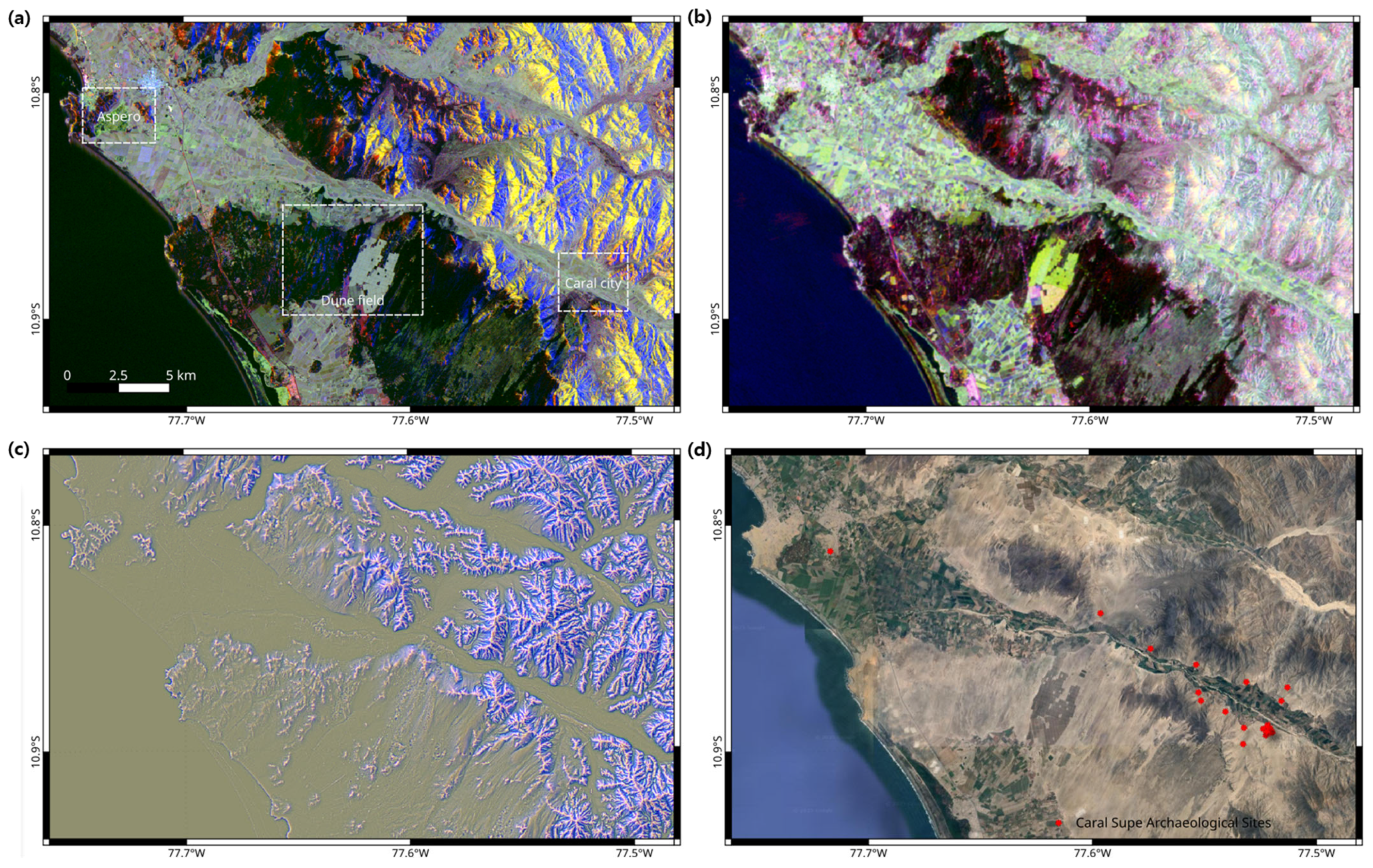
Although the single-band SR products are of high quality, they do not always allow straightforward visual interpretation of archeological features. To overcome this limitation, we constructed multi-channel composite images integrating variations in polarization, viewing geometry, and acquisition date. These SR composites are shown in Figure 6: S-1 ascending VV/VH and descending VH in Figure 6a; PALSAR 2020s HH/VH combined with 2010s HV in Figure 6b; and three SR DEM-derived parameters—roughness (search radius 4), MSRM (40–200 m band-pass), and LRM in Figure 6c as RGB composites.

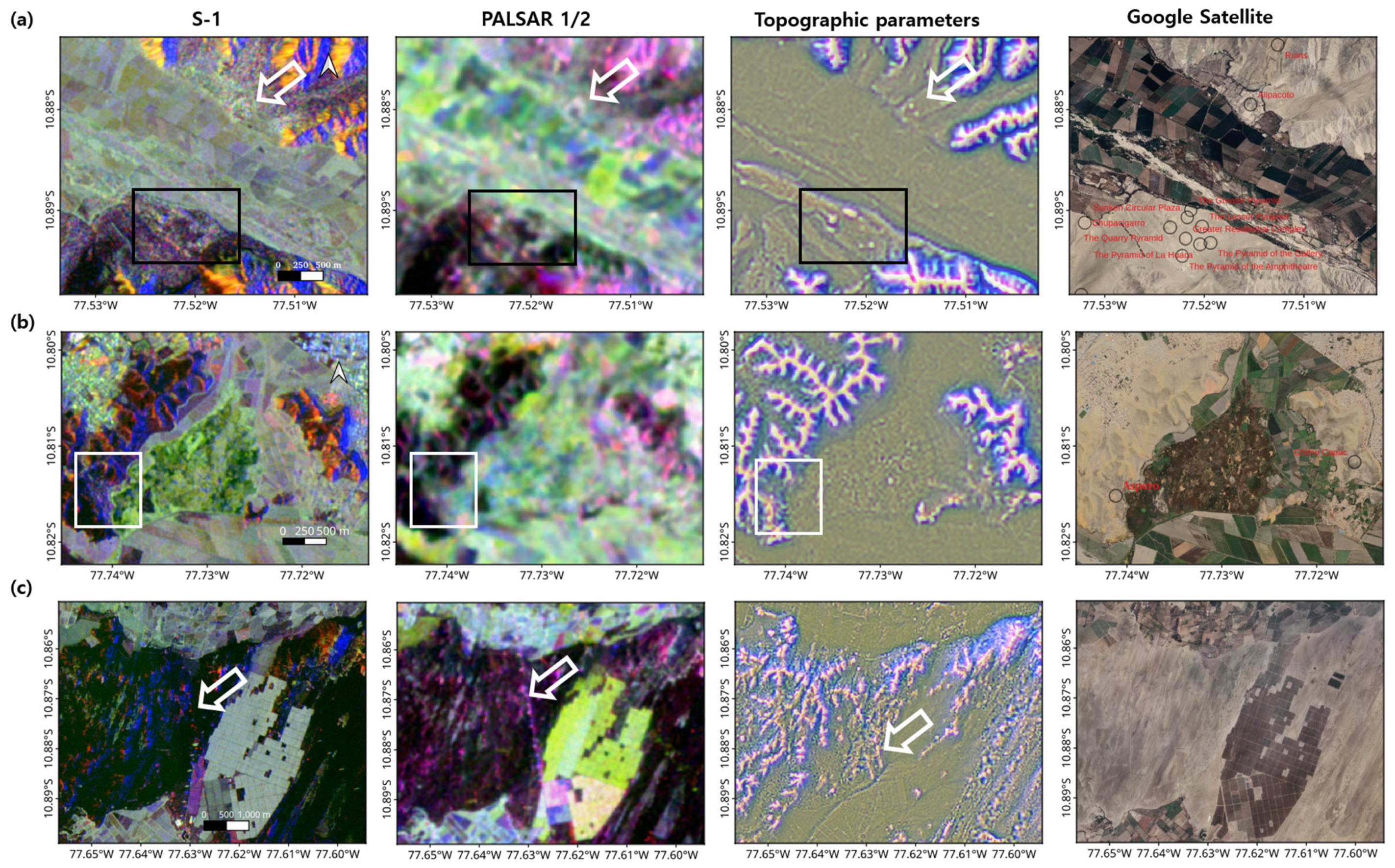
Figure 6. Composite images from SR datasets. (a) S-1 SR image composites with a resolution of 1.47 m (SR images in ascending VV in R band, ascending VH in G band, and descending VH in B band). (b) PALSAR SR image composites with a resolution of 5 m (SR images in 2020’s HH mode in R band, 2020’s HV mode in G band, and 2010’s HH mode in B band). (c) SR DEM’s topographic parameters in RGB channels with a resolution of 5 m and roughness with a search radius of 4 in R band, MSRM (90 m < band-pass filter size < 400 m) in G band, and LRM (radius = 90 m) in B band. (d) Google Satellite images and major Caral–Supe sites.

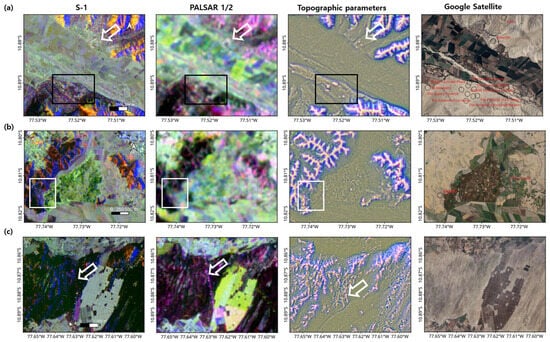
Figure 7 illustrates the performance of these composites across three major sub-regions: Caral City in Figure 7a, Aspero in Figure 7b, and the coastal dune field in Figure 7c. In both Caral and Aspero, architectural features are clearly delineated in SR S-1 and in topographic derivatives generated from the SR DEM. Furthermore, both S-1 and PALSAR SR products reveal distinct outlines of the underlying base terrain, suggesting that these centers were constructed on artificially modified or naturally level surfaces.

Figure 7. (a) Composite images of SR S-1, SR PALSAR-1/2, topographic parameters from SR DEM, and corresponding Google satellite image around Caral City. Boxed area assigned the major part of Caral City and arrowed to the archeological structures in Allpacoto. (b) Composite images of SR S-1, SR PALSAR, topographic parameters from SR DEM, and corresponding Google satellite image around Aspero (white boxed area). (c) Composite images of SR S-1, SR PALSAR, topographic parameters from SR DEM, and corresponding Google satellite image around the coastal dune field. Arrow assigns the trail of discovered subsurface structure, perhaps the pipelines. Refer to Figure 5a for their locations and extents. Image band compositions as described in Figure 6.

Finally, the penetration capability of L-band SAR is demonstrated in Figure 7c, which shows a shallow subsurface linear feature, perhaps interpreted as a modern pipeline. This observation further underscores the value of SAR, particularly L-band systems, for archeological prospection and detection of shallow subsurface structures.

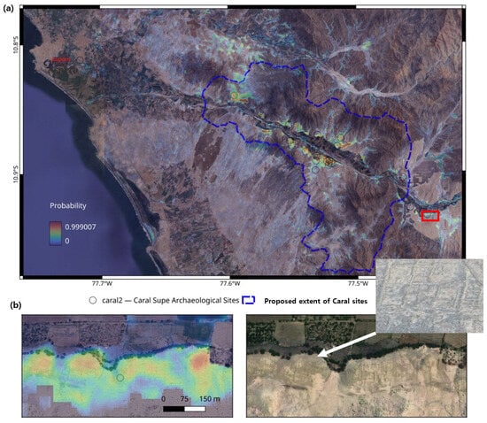
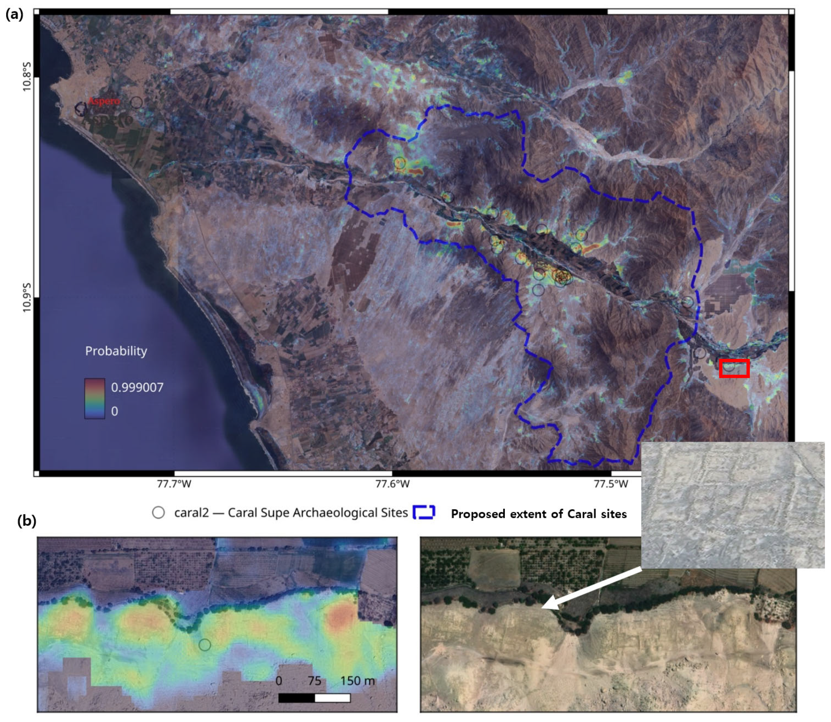
Figure 8 shows classification results from multiband input, a total of 11 bands consisting of four bands from PALSAR, four bands from S-1, and three bands from DEM products, and the Attention U-Net algorithm as a probability map for Caral–Supe sites. Around 700 km² of potential archeological areas were assessed, with probabilities ranging from 0 to 100 using training data covering 2.3 km² digitized from the UNESCO map. In addition, invalid portions for classification are defined by a built-up mask and high-sloped terrain (>30 deg). High-probability areas correspond well to known archeological sites and the Penico area, as validation data in Figure 8b. Additional probability maps using different data combinations are evaluated in the following section.

Figure 8. Probability maps of archeological structures in the Caral–Supe sites (a,b) indicate local artificial features of unknown chronology through comparisons with the regional probability map (right) and Bing image (left) in Penico (red boxed area in (a)).

5. Interpretation and Validation

First, we evaluated the quality of the SR images relative to the corresponding original SAR images using the Peak Signal-to-Noise Ratio (PSNR) and Structural Similarity Index Measure (SSIM) [68] (Table 2). We also assessed the products in the pre-processing stage—namely the tr-SVD products for S-1 and the enhanced Lee-filtered PALSAR images. Although the tr-SVD images show relatively low PSNR and SSIM values, visual inspection confirms substantial noise reduction. This outcome was expected because tr-SVD intentionally suppresses temporal components in the packet-based approach, thereby reducing similarity to the original data but producing cleaner inputs for subsequent SR processing. After applying SR imaging to the tr-SVD results, both PSNR (>25) and SSIM (>0.8) improved markedly. These results support the effectiveness of our stepwise workflow, i.e., original to tr-SVD and to the SR image, for removing temporal noise while enhancing the spatial fidelity of meaningful signals, including partially buried archeological features. The enhanced Lee filter presents higher metrics, PNSRs better than 30 and SSIMs better than 0.85 in Table 2 (b) because it clearly suppresses noises; however, it may also remove subtle signals relevant to archeological interpretation. Thus, its performance should be interpreted carefully, and it should primarily serve as an alternative when the TS data required for tr-SVD is unavailable. In general, the SR imaging metrics obtained in this study are comparable to or better than values reported in earlier remote sensing applications using both optical and SAR data [19,69,70], with overall PNSRs around 25 to 30 and SSIMs better than 0.8. Certain polarization modes, such as VV for S-1 and HH for PALSAR, along with ascending viewing geometry, consistently provided higher-quality results and were therefore more effective for a visual analysis of archeological features.

Table 2. Evaluation of SR images by PNSR and SSIM.

(a) s-1
SR vs. tr-SVD images	PNSR	SSIM	Tr-SVD vs. original images	PNSR	SSIM
Ascending VV	30.392	0.872	Ascending VV	16.783	0.558
Ascending VH	23.281	0.782	Ascending VH	13.974	0.738
Descending VV	27.830	0.882	Descending VV	13.991	0.634
Descending VH	25.777	0.860	Descending VH	13.158	0.533
(b) PALSAR-1/2 *Elee means Enhanced Lee filter
SR vs. *Elee images	PNSR	SSIM	Elee vs. original images	PNSR	SSIM
2010s HH	24.648	0.913	2010s HH	33.8706	0.866
2020s HH	25.189	0.867	2020s HH	33.913	0.872
2010s HV	29.067	0.901	2010s HV	30.415	0.946
2020s HV	27.034	0.895	2020s HV	30.044	0.934

*Elee means the enhanced Lee-filtered images.

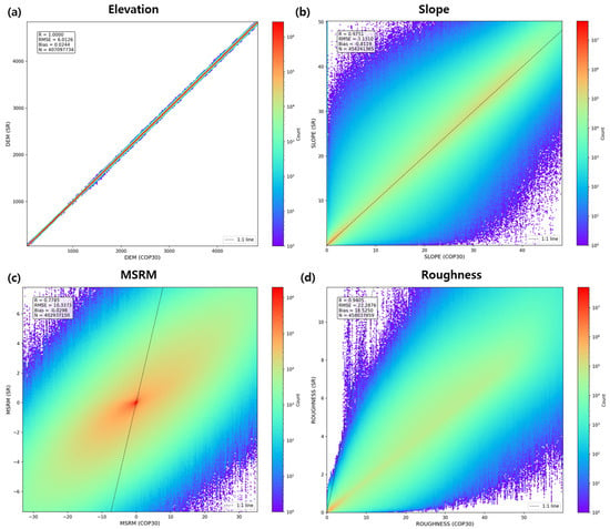
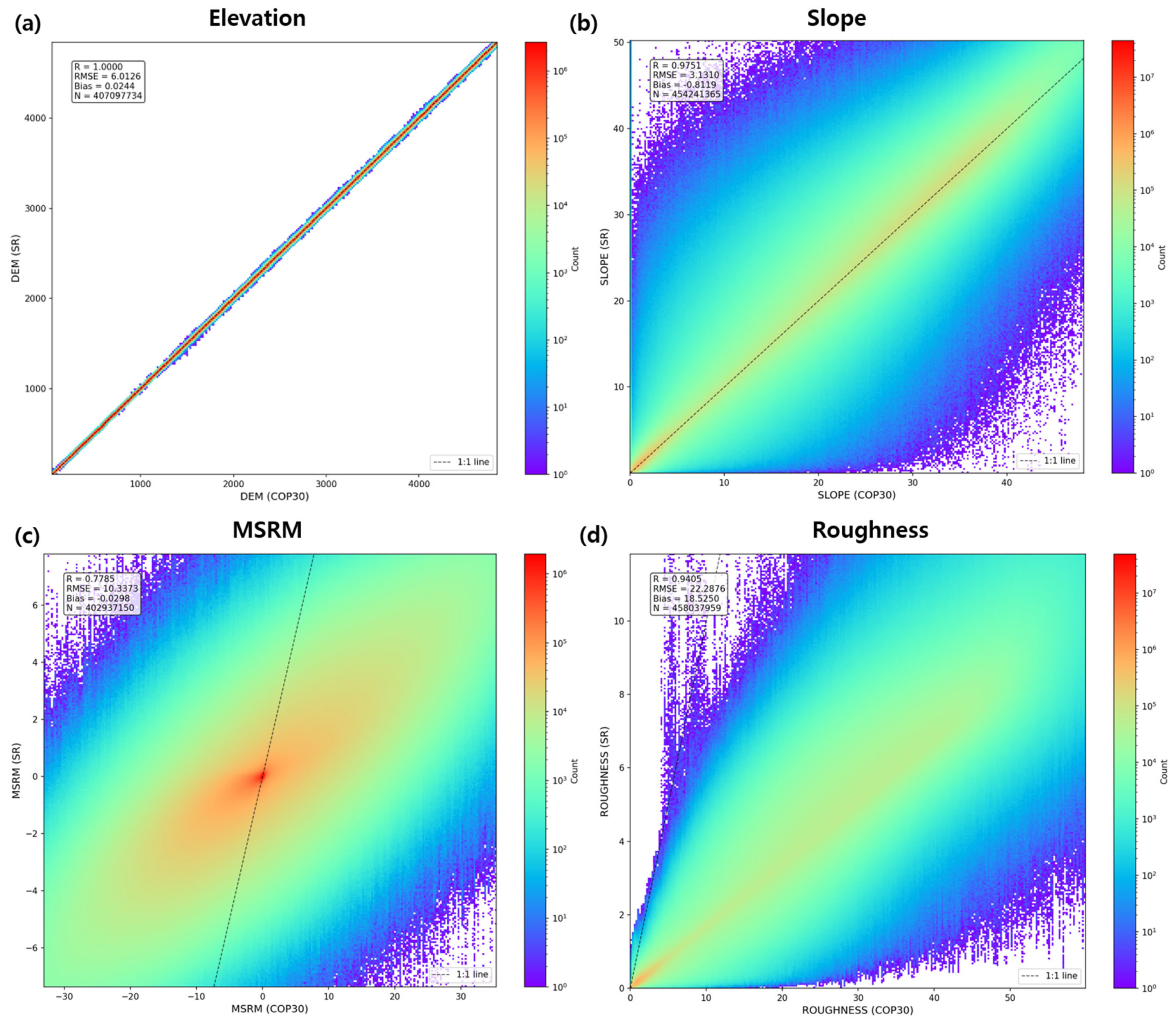
Because PSNR and SSIM are not suitable for evaluating SR DEM quality, we examined the correlation between the COP 30 DEM and SR DEM, along with their derivative products (Figure 9). For elevation datasets, the key requirement is that the SR DEM preserve the original elevation range while providing enhanced topographic detail without introducing artificial height values. As shown in Figure 9a,b, the elevation range remains highly stable even after SR processing. In contrast, nonlinear topographic derivatives—such as MSRM and roughness—exhibit greater dispersion, though they still maintain strong correlation (Figure 9c,d). These results indicate that the SR DEM algorithm reliably maintains elevation integrity while offering improved representation of fine-scale geomorphological features, as already shown in Figure 5, Figure 6 and Figure 7.

Figure 9. The correlations between COP-30 DEM products vs. SR DEM products. (a) Elevations of SR DEM and COP 30, (b) slopes of SR DEM and COP 30, (c) MSRMs of SR DEM and COP 30, and (d) roughness of SR DEM and COP 30.

Figure 8 already demonstrates strong agreement with known archeological features; however, a more rigorous evaluation of the Attention U-Net classification performance is necessary. To this end, six classification scenarios were designed to systematically assess the contribution of each input configuration. Specifically, the following input combinations were independently forwarded to the Attention U-Net architecture: (1) eleven bands comprising SAR and DEM-derived products at the original DEM’s 30 m resolution; (2) eight bands from 30 m resampled SAR images; (3) three bands constructed exclusively from DEM-derived products at the original resolution; (4) eleven bands comprising SR SAR together with SR DEM-derived products; (5) eight bands from SR SAR images; (6) three bands constructed from SR DEM-derived products. In all experiments, 50% of the digitized archeological features from the UNESCO map were used for training, while the remaining 50% were reserved for validation.

Given that the classification output represents continuous probability rather than a hard-threshold prediction, conventional confusion matrix metrics are inadequate for capturing the full extent of model performance. We therefore adopt a soft confusion matrix formulation [71], defined as follows:

$$\mathit{sTP}={\sum }_i{y}_i p_i$$

$$\mathit{sFN}={\sum }_i{y}_i(1-p_i)$$

$$\mathit{sFP}={\sum }_i(1-y_i)p_i$$

$$\mathit{sTN}={\sum }_i(1-y_i)(1-p_i)$$

(4)

where $y_i$ is the ground truth label of binary pixel i, and $p_i$ represents the corresponding predicted probability from the output map. In this framework, soft true positive (sTP) quantifies the cumulative probability mass correctly assigned to positive pixels, soft false negative (sFN) captures the probability mass that was missed among true positive pixels, soft false positive (sFP) measures the probability mass erroneously assigned to true negative pixels, and soft true negative (sTN) reflects the probability mass correctly withheld from negative pixels.

Building upon the soft confusion matrix, we extend the standard evaluation metrics [72] to their probabilistic counterparts as follows:

$$sAccuracy={\displaystyle \frac{sTP+sTN}{sTP+sTN+sFP+sFN}}$$

$$sPrecision={\displaystyle \frac{sTP}{sTP+sFP}}$$

$$sRecall={\displaystyle \frac{sTP}{sTP+sFN}}$$

$$sSpecificity={\displaystyle \frac{sTN}{sTN+sFP}}$$

$$sFPR={\displaystyle \frac{sFP}{sFP+sTN}}$$

$$sFNR={\displaystyle \frac{sFN}{sFN+sTP}}$$

$$sF1={\displaystyle \frac{2\ast sPrecision\ast sRecall}{sPrecision+sRecall}}$$

(5)

where soft accuracy (sAccuracy) represents the expected fraction of correctly classified pixels in probability-weighted terms. Soft precision (sPrecision) is the expected degree of predicted positives, indicating the degree to which positive predictions are free from false alarms. Soft recall (sRecall) measures the expected coverage of true positives, reflecting the model’s capacity to detect actual archeological features. Soft specificity (sSpecificity) describes the expected correctness over true negative pixels. The soft false positive rate (sFPR) provides the expected false alarm rate, while the soft false negative rate (sFNR) quantifies the expected miss rate, both expressed as probability mass. Finally, the soft F1 Score (sF1) is the harmonic average of soft precision and soft recall, providing a balanced summary of the trade-off between prediction purity and detection coverage using probability-weighted counts.

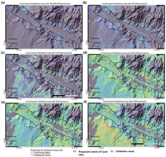
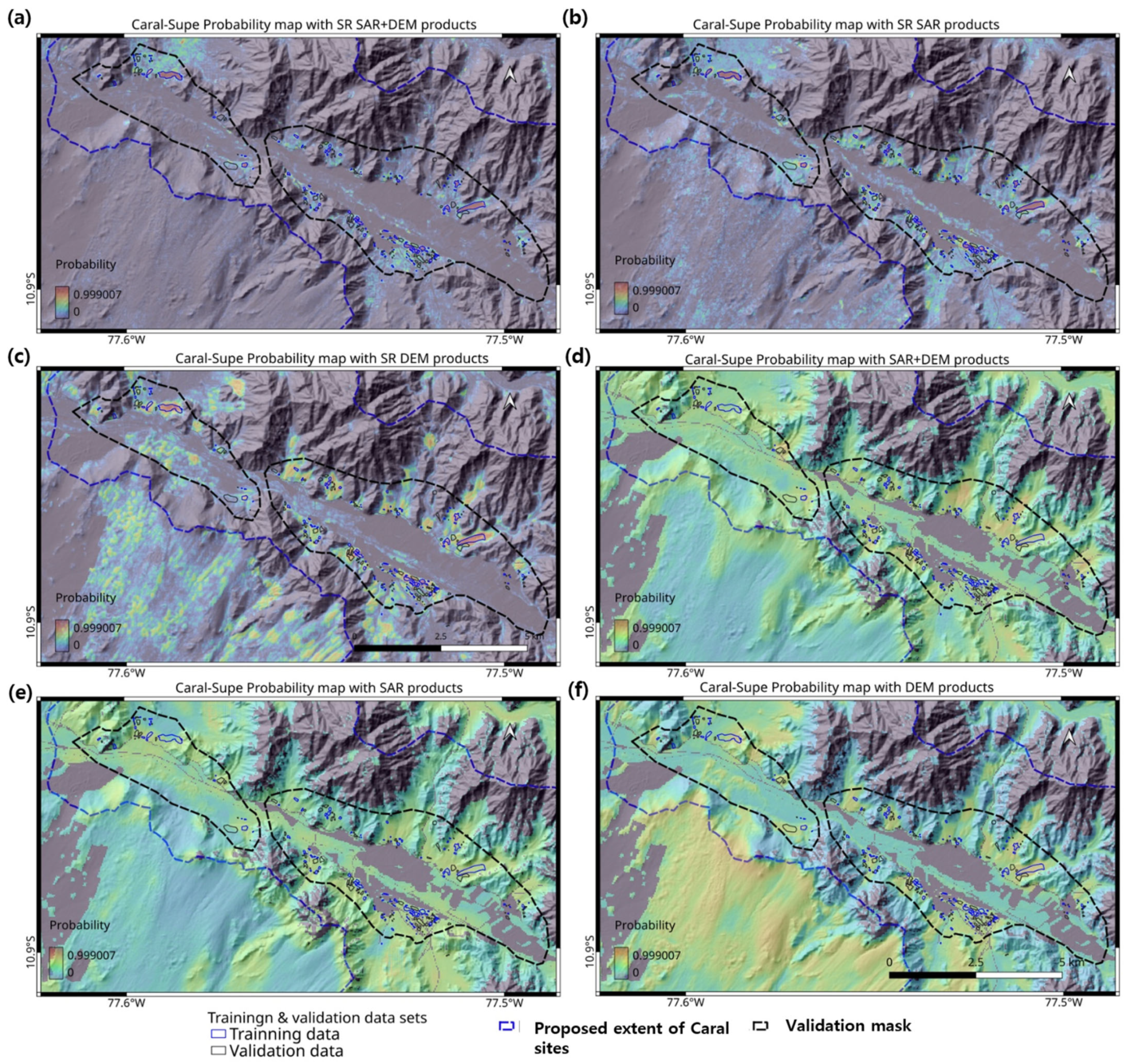
One significant issue in evaluating performance with an approach involving multiple scenarios and a confusion matrix is the incompleteness of validation data. As employed validation data, i.e., the digitized outlines from the UNESCO map, do not guarantee that all archeological sites are included, the negative side metric may affect results. Thus, we introduced a narrow mask around the validation data and calculated metrics within it (Figure 10).

Figure 10. Probability maps of archeological structures at the Caral–Supe sites under six different scenarios. (a) Probability map generated from SR SAR images and SR DEM products. (b) Probability map derived from SR SAR images. (c) Probability map based on SR DEM products. (d) Probability map utilizing 30 m resolution SAR images and DEM products. (e) Probability map from 30 m resolution SAR images. (f) Probability map using 30 m resolution DEM products.

Table 3 presents the evaluation results based on these soft metric definitions across all six scenarios. The superiority of SR products for the detection of archeological features is very obvious. SR products improve all feature sets’ precision to 70–85%, F1 gains to 47–68%, and FPR reductions to 54–78%. sRecall drops because enhanced models produce more focused probability maps. Although SR DEM products have slightly better metrics except for the sAccuracy, the adaptability of input datasets is not very clear from the metrics. Therefore, it is necessary to compare the visualized products shown in Figure 10. Figure 10d–f clearly demonstrate that the original 30 m products are not applicable for the feature classification. The probability range between archeological features and natural landscapes is only 20–30%; thus, in all three cases, it is not possible to focus on specific areas of interest from an archeological perspective. On the other hand, Figure 10c also shows the limitations of SR DEM product-based detection. It has many clear false positives over the natural topographic outliners, such as sand dunes. Despite good assessment metrics, the SR DEM-only products could not provide meaningful information for investigating archeological features. Figure 10a,b show similar patterns to each other, but the case of SR SAR images with SR DEM products in Figure 10a shows more localized and less sensitivity to topographic outliers. The results show that combining SR multiband DEM data with SAR channels is the most effective method for identifying archeological sites, confirming the superior performance of SR SAR images plus SR DEM products in feature classification.

Table 3. Evaluation metrics for six different scenarios.

Metric	SAR + DEM (SR)	SAR Only (SR)	DEM Only (SR)	SAR + DEM (30 m)	SAR Only (30 m)	DEM Only (30 m)
sTP	3457.20	5061.29	7097.90	254.8	233.29	245.88
sFN	15,983.80	14,379.71	12,343.10	284.2	305.71	293.12
sFP	85,321.96	119,666.73	157,522.06	10,882.44	10,416.16	9607.39
sTN	1,104,407.04	1,070,062.27	1,032,206.94	22,159.56	22,625.84	23,434.61
sAccuracy	0.916	0.889	0.859	0.667	0.681	0.705
sPrecision	0.039	0.041	0.043	0.023	0.022	0.025
sRecall	0.178	0.260	0.365	0.473	0.433	0.456
sF1	0.064	0.070	0.077	0.044	0.042	0.047
sSpecificity	0.928	0.899	0.868	0.677	0.685	0.709
sFPR	0.072	0.100	0.132	0.329	0.315	0.291
sFNR	0.822	0.740	0.635	0.527	0.567	0.544

The multiband reconstruction using L/C-band SAR images and DEM products demonstrates high efficiency, as evidenced by both the metrics in Table 3 and the observations in Figure 7, which show the key information provided by various bandwidths of SAR images and DEM products. Figure 7c, captured over a dune field, highlights the primary contributions of each input image channel. L-band SAR images reveal deeply buried surface structures such as modern pipelines at estimated depths of 1–2 m, while C-band images show backscattering from textured surfaces produced by irregular planes on or near the surface. DEM products effectively represent terrain features across multiple pixel sizes, including dunes and embankments (Figure 7a,c). Consequently, an efficient classifier can process the diverse features presented at varying depths and surface roughness levels. Such advantages are not achievable through data mining when relying solely on optical images, LiDAR, or other single-band image products. It should be noted that generating a probability map covering 700 km² at a 5 m resolution is also not practical with an aerial remote sensing sensor or LiDAR.

Our processed datasets yield several preliminary clues related to the Caral–Supe civilization. These observations remain tentative and require confirmation through further discussion with on-site archeologists as well as additional ground surveys and datasets:

(1)

The data suggests the presence of numerous yet-undiscovered archeological structures, particularly along the Supe Valley. Many of these features appear consistent with architectural patterns known from Caral–Supe sites. It also implies that the Caral–Supe civilization may have been more widespread than previously believed based on existing archeological discoveries [73]. There could be possible sites in the northern valley of the Supe, as well as in the adjoining piedmont areas.

(2)

Although the detected signals are weak, several potential anthropogenic structures may be buried in the shallow subsurface along the coastline and within dune-covered hillsides. If these features are indeed associated with the Caral–Supe civilization, they could offer support for hypotheses linking the civilization’s spatial shifts to climate-related environmental change [74,75]. Residents in coastal regions who relied on fishing, as well as those from the Supe Valley engaged in agriculture, may have utilized Aspero—acknowledged as a trading hub—for the exchange of their products.

(3)

A substantial portion of surface architecture appears damaged or partially to fully buried, resulting in weak signatures in SAR imagery. Although long-term natural erosion is a probable contributing factor, it is also important to consider the potential impacts of historical natural disasters such as earthquakes and landslides, which may have influenced the decline of the Caral–Supe civilization [75].

Given this level of accuracy, we are confident that our methods successfully detected a large portion of archeological structures that may date to the Caral–Supe period.

6. Conclusions

This study demonstrates how SR imaging techniques, combined with publicly available datasets, can be effectively applied to archeological investigations. By generating SR imagery and integrating it into deep learning-based classification algorithms, we addressed the limitations of public-domain data in identifying individual archeological structures and their broader environmental contexts.

Applied to the ancient Caral–Supe region, our approach proved capable of delineating specific architectural features as well as associated geomorphological settings. Further processing of the SR products through deep learning-based classification revealed additional potential anthropogenic structures that had not been previously documented. This advancement is largely attributed to SAR’s ability to detect shallow subsurface features and to extract detailed three-dimensional information together with SR-enhanced topography. Such findings may suggest a larger population and greater spatial extent for the Caral–Supe civilization than currently recognized.

Although direct visual identification of archeological features from contemporary public SAR datasets remains limited, ongoing missions, such as the NASA–ISRO Synthetic Aperture Radar (NISAR) and ESA’s BIOMASS mission, combined with SR methodologies, are expected to offer significantly improved opportunities for archeological applications.

References

- Luo, L.; Wang, X.; Guo, H.; Lasaponara, R.; Zong, X.; Masini, N.; Wang, G.; Shi, P.; Khatteli, H.; Chen, F. Airborne and spaceborne remote sensing for archaeological and cultural heritage applications: A review of the century (1907–2017). Remote Sens. Environ. 2019, 232, 111280. [Google Scholar] [CrossRef] [Scilit]
- Lasaponara, R.; Masini, N. Satellite remote sensing in archaeology: Past, present and future perspectives. J. Archaeol. Sci. 2011, 38, 1995–2002. [Google Scholar] [CrossRef] [Scilit]
- Adamopoulos, E.; Rinaudo, F. UAS-based archaeological remote sensing: Review, meta-analysis and state-of-the-art. Drones 2020, 4, 46. [Google Scholar] [CrossRef] [Scilit]
- Tapete, D.; Traviglia, A.; Delpozzo, E.; Cigna, F. Regional-scale systematic mapping of archaeological mounds and detection of looting using COSMO-SkyMed high resolution DEM and satellite imagery. Remote Sens. 2021, 13, 3106. [Google Scholar] [CrossRef] [Scilit]
- Corrie, R.K. Detection of ancient Egyptian archaeological sites using satellite remote sensing and digital image processing. In Proceedings of the Earth Resources and Environmental Remote Sensing/GIS Applications II, Prague, Czech Republic, 19–22 September 2011; pp. 270–288. [Google Scholar]
- Ur, J. Sennacherib’s northern Assyrian canals: New insights from satellite imagery and aerial photography. Iraq 2005, 67, 317–345. [Google Scholar] [CrossRef] [Scilit]
- Zaghloul, E.; Hassan, S.; El-Dein, A.B.; Elbeih, S. Detection of ancient irrigation canals of Deir El-Hagar playa, Dakhla Oasis, Egypt, using Egyptsat-1 data. Egypt. J. Remote Sens. Space Sci. 2013, 16, 153–161. [Google Scholar] [CrossRef] [Scilit]
- Parcak, S. Satellite remote sensing methods for monitoring archaeological tells in the Middle East. J. Field Archaeol. 2007, 32, 65–81. [Google Scholar] [CrossRef] [Scilit]
- Hammer, E.; FitzPatrick, M.; Ur, J. Succeeding CORONA: Declassified HEXAGON intelligence imagery for archaeological and historical research. Antiquity 2022, 96, 679–695. [Google Scholar] [CrossRef] [Scilit]
- Orengo, H.A.; Petrie, C.A. Multi-scale relief model (MSRM): A new algorithm for the visualization of subtle topographic change of variable size in digital elevation models. Earth Surf. Process. Landf. 2018, 43, 1361–1369. [Google Scholar] [CrossRef] [Scilit]
- Kim, J. Tracing Archaeological Places via the Context of Paleo Geomorphic Footprints Using SAR/InSAR Data Fusion: A Case on Southern Mesopotamia. Remote Sens. 2023, 15, 1636. [Google Scholar] [CrossRef] [Scilit]
- Franks, S.; Rengarajan, R. Evaluation of Copernicus DEM and comparison to the DEM used for Landsat Collection-2 processing. Remote Sens. 2023, 15, 2509. [Google Scholar] [CrossRef] [Scilit]
- Freeman, A.; Durden, S.L. A three-component scattering model for polarimetric SAR data. IEEE Trans. Geosci. Remote Sens. 2002, 36, 963–973. [Google Scholar] [CrossRef] [Scilit]
- Singh, A.; Niranjannaik, M.; Kumar, S.; Gaurav, K. Comparison of different dielectric models to estimate penetration depth of l-and s-band sar signals into the ground surface. Geographies 2022, 2, 734–742. [Google Scholar] [CrossRef] [Scilit]
- El Hajj, M.; Baghdadi, N.; Bazzi, H.; Zribi, M. Penetration analysis of SAR signals in the C and L bands for wheat, maize, and grasslands. Remote Sens. 2018, 11, 31. [Google Scholar] [CrossRef] [Scilit]
- Van Gasselt, S.; Kim, J.R.; Choi, Y.-S.; Kim, J. The Oasis impact structure, Libya: Geological characteristics from ALOS PALSAR-2 data interpretation. Earth Planets Space 2017, 69, 35. [Google Scholar] [CrossRef] [Scilit]
- Paillou, P.; Lopez, S.; Farr, T.; Rosenqvist, A. Mapping subsurface geology in Sahara using L-Band SAR: First results from the ALOS/PALSAR imaging radar. IEEE J. Sel. Top. Appl. Earth Obs. Remote Sens. 2010, 3, 632–636. [Google Scholar] [CrossRef] [Scilit]
- Paillou, P.; Grandjean, G.; Baghdadi, N.; Heggy, E.; August-Bernex, T.; Achache, J. Subsurface imaging in south-central Egypt using low-frequency radar: Bir Safsaf revisited. IEEE Trans. Geosci. Remote Sens. 2003, 41, 1672–1684. [Google Scholar] [CrossRef]
- Wang, L.; Zheng, M.; Du, W.; Wei, M.; Li, L. Super-resolution SAR image reconstruction via generative adversarial network. In Proceedings of the 2018 12th International Symposium on Antennas, Propagation and EM Theory (ISAPE), Hangzhou, China, 3–6 December 2018; pp. 1–4. [Google Scholar]
- Wang, X.; Yu, K.; Wu, S.; Gu, J.; Liu, Y.; Dong, C.; Qiao, Y.; Change Loy, C. Esrgan: Enhanced super-resolution generative adversarial networks. In Proceedings of the European Conference on Computer Vision (ECCV) Workshops, Munich, Germany, 8–14 September 2018. [Google Scholar]
- Solis, R.S.; Haas, J.; Creamer, W. Dating Caral, a preceramic site in the Supe Valley on the central coast of Peru. Science 2001, 292, 723–726. [Google Scholar] [CrossRef] [Scilit] [PubMed]
- Solis, R.S. America’s first city? The case of Late Archaic Caral. In Andean Archaeology III: North and South; Springer: Berlin/Heidelberg, Germany, 2006; pp. 28–66. [Google Scholar]
- Moseley, M.E. Maritime foundations and multilinear evolution: Retrospect and prospect. Andean Past 1992, 3, 5. [Google Scholar]
- Tozer, B.; Sandwell, D.T.; Smith, W.H.; Olson, C.; Beale, J.R.; Wessel, P. Global bathymetry and topography at 15 arc sec: SRTM15+. Earth Space Sci. 2019, 6, 1847–1864. [Google Scholar] [CrossRef] [Scilit]
- Haas, J.; Creamer, W.; Ruiz, A. Power and the emergence of complex polities in the Peruvian Preceramic. Archeol. Pap. Am. Anthropol. Assoc. 2004, 14, 37–52. [Google Scholar] [CrossRef] [Scilit]
- Haas, J.; Creamer, W.; Ruiz, A. Dating the Late Archaic occupation of the Norte Chico region in Peru. Nature 2004, 432, 1020–1023. [Google Scholar] [CrossRef] [Scilit]
- Benfer, B.; Burger, R.L.; Rosenswig, R.M. Monumental architecture arising from an early astronomical-religious complex in Peru, 2200–1750 BC. In Monumentality in the Americas; Rosenswig, R.M., Burger, R.L., Eds.; University Press of Florida: Gainesville, FL, USA, 2012; pp. 313–363. [Google Scholar]
- Oakland, A. Middle Horizon textiles from Chimu Capac, Supe Valley, Peru. In PreColumbian Textile Conference VIII/Jornadas de Textiles PreColombinos VIII (2019); Zea Books: Lincoln, NE, USA, 2020. [Google Scholar]
- Ortloff, C.; Moseley, M. 2600–1800 BCE Caral. Ñawpa Pacha 2013, 32, 189–206. [Google Scholar] [CrossRef] [Scilit]
- Geudtner, D.; Torres, R.; Snoeij, P.; Davidson, M.; Rommen, B. Sentinel-1 system capabilities and applications. In Proceedings of the 2014 IEEE Geoscience and Remote Sensing Symposium, Quebec City, QC, Canada, 13–18 July 2014; pp. 1457–1460. [Google Scholar]
- Kankaku, Y.; Suzuki, S.; Osawa, Y. ALOS-2 mission and development status. In Proceedings of the 2013 IEEE International Geoscience and Remote Sensing Symposium-IGARSS, Melbourne, Australia, 21–26 July 2013; pp. 2396–2399. [Google Scholar]
- Shimada, M.; Ohtaki, T. Generating large-scale high-quality SAR mosaic datasets: Application to PALSAR data for global monitoring. IEEE J. Sel. Top. Appl. Earth Obs. Remote Sens. 2010, 3, 637–656. [Google Scholar] [CrossRef] [Scilit]
- Japan Aerospace Exploration Agency. Global 25m Resolution PALSAR-2/PALSAR Mosaic and Forest/Non-Forest Map (FNF); Japan Aerospace Exploration Agency: Tokyo, Japan, 2010; Available online: https://www.eorc.jaxa.jp/ALOS/en/dataset/fnf_e.htm (accessed on 1 March 2026).
- McCauley, J.F.; Schaber, G.G.; Breed, C.S.; Grolier, M.J.; Haynes, C.V.; Issawi, B.; Elachi, C.; Blom, R. Subsurface valleys and geoarcheology of the eastern Sahara revealed by shuttle radar. Science 1982, 218, 1004–1020. [Google Scholar] [CrossRef] [Scilit]
- Fluhrer, A.; Jagdhuber, T.; Tabatabaeenejad, A.; Alemohammad, H.; Montzka, C.; Friedl, P.; Forootan, E.; Kunstmann, H. Remote sensing of complex permittivity and penetration depth of soils using P-band SAR polarimetry. Remote Sens. 2022, 14, 2755. [Google Scholar] [CrossRef] [Scilit]
- Zhu, J.; Liu, G.; Zhao, R.; Ding, X.; Fu, H. ML based approach for inverting penetration depth of SAR signals over large desert areas. Remote Sens. Environ. 2023, 295, 113643. [Google Scholar] [CrossRef] [Scilit]
- Riegler, G.; Hennig, S.; Weber, M. WorldDEM–A novel global foundation layer. Int. Arch. Photogramm. Remote Sens. Spat. Inf. Sci. 2015, 40, 183–187. [Google Scholar] [CrossRef] [Scilit]
- Krieger, G.; Moreira, A.; Fiedler, H.; Hajnsek, I.; Werner, M.; Younis, M.; Zink, M. TanDEM-X: A satellite formation for high-resolution SAR interferometry. IEEE Trans. Geosci. Remote Sens. 2007, 45, 3317–3341. [Google Scholar] [CrossRef] [Scilit]
- Becek, K.; Koppe, W.; Kutoğlu, Ş.H. Evaluation of vertical accuracy of the WorldDEM™ using the runway method. Remote Sens. 2016, 8, 934. [Google Scholar] [CrossRef] [Scilit]
- Frost, V.S.; Stiles, J.A.; Shanmugan, K.S.; Holtzman, J.C. A model for radar images and its application to adaptive digital filtering of multiplicative noise. IEEE Trans. Pattern Anal. Mach. Intell. 1982, PAMI-4, 157–166. [Google Scholar] [CrossRef] [Scilit]
- Yun, H.-W.; Kim, J.-R.; Choi, Y.-S.; Lin, S.-Y. Analyses of time series InSAR signatures for land cover classification: Case studies over dense forestry areas with L-band SAR images. Sensors 2019, 19, 2830. [Google Scholar] [CrossRef] [Scilit] [PubMed]
- Hansen, P.C. Truncated singular value decomposition solutions to discrete ill-posed problems with ill-determined numerical rank. SIAM J. Sci. Stat. Comput. 1990, 11, 503–518. [Google Scholar] [CrossRef] [Scilit]
- Greenspan, H. Super-resolution in medical imaging. Comput. J. 2009, 52, 43–63. [Google Scholar] [CrossRef] [Scilit]
- Puschmann, K.G.; Kneer, F. On super-resolution in astronomical imaging. Astron. Astrophys. 2005, 436, 373–378. [Google Scholar] [CrossRef] [Scilit]
- Yang, D.; Li, Z.; Xia, Y.; Chen, Z. Remote sensing image super-resolution: Challenges and approaches. In Proceedings of the 2015 IEEE International Conference on Digital Signal Processing (DSP), Singapore, 21–24 July 2015; pp. 196–200. [Google Scholar]
- Bashir, S.M.A.; Wang, Y.; Khan, M.; Niu, Y. A comprehensive review of deep learning-based single image super-resolution. PeerJ Comput. Sci. 2021, 7, e621. [Google Scholar] [CrossRef] [Scilit]
- Irani, M.; Peleg, S. Super resolution from image sequences. In Proceedings of the 10th International Conference on Pattern Recognition, Atlantic City, NJ, USA, 16–21 June 1990; pp. 115–120. [Google Scholar]
- Panda, S.S.; Prasad, M.; Jena, G. POCS based super-resolution image reconstruction using an adaptive regularization parameter. arXiv 2011, arXiv:1112.1484. [Google Scholar] [CrossRef] [Scilit]
- Ledig, C.; Theis, L.; Huszár, F.; Caballero, J.; Cunningham, A.; Acosta, A.; Aitken, A.; Tejani, A.; Totz, J.; Wang, Z. Photo-realistic single image super-resolution using a generative adversarial network. In Proceedings of the IEEE Conference on Computer Vision and Pattern Recognition, Honolulu, HI, USA, 21–27 July 2017; pp. 4681–4690. [Google Scholar]
- Simonyan, K.; Zisserman, A. Very deep convolutional networks for large-scale image recognition. arXiv 2014, arXiv:1409.1556. [Google Scholar]
- Isola, P.; Zhu, J.-Y.; Zhou, T.; Efros, A.A. Image-to-image translation with conditional adversarial networks. In Proceedings of the IEEE Conference on Computer Vision and Pattern Recognition, Honolulu, HI, USA, 21–27 July 2017; pp. 1125–1134. [Google Scholar]
- Aitken, A.; Ledig, C.; Theis, L.; Caballero, J.; Wang, Z.; Shi, W. Checkerboard artifact free sub-pixel convolution: A note on sub-pixel convolution, resize convolution and convolution resize. arXiv 2017, arXiv:1707.02937. [Google Scholar]
- Hu, G.; Jiang, Y.; Li, S.; Xiong, L.; Tang, G.; Mariethoz, G. Super-resolution of digital elevation models by using multiple-point statistics and training image selection. Comput. Geosci. 2024, 191, 105688. [Google Scholar] [CrossRef] [Scilit]
- Chen, Z.; Wang, X.; Xu, Z.; Hou, W. Convolutional neural network based dem super resolution. Int. Arch. Photogramm. Remote Sens. Spat. Inf. Sci. 2016, 41, 247–250. [Google Scholar] [CrossRef] [Scilit]
- Demiray, B.Z.; Sit, M.; Demir, I. D-SRGAN: DEM super-resolution with generative adversarial networks. SN Comput. Sci. 2021, 2, 48. [Google Scholar] [CrossRef] [Scilit]
- Hengl, T.; Bajat, B.; Blagojević, D.; Reuter, H.I. Geostatistical modeling of topography using auxiliary maps. Comput. Geosci. 2008, 34, 1886–1899. [Google Scholar] [CrossRef] [Scilit]
- Kyriakidis, P.C. A geostatistical framework for area-to-point spatial interpolation. Geogr. Anal. 2004, 36, 259–289. [Google Scholar]
- Zhou, Q.; Chen, S.; Liu, J.; Tang, X. Edge-preserving single image super-resolution. In Proceedings of the 19th ACM International Conference on Multimedia, Scottsdale, AZ, USA, 28 November–1 December 2011; pp. 1037–1040. [Google Scholar]
- Hesse, R. LiDAR-derived Local Relief Models–a new tool for archaeological prospection. Archaeol. Prospect. 2010, 17, 67–72. [Google Scholar] [CrossRef] [Scilit]
- Bekker, J.; Davis, J. Learning from positive and unlabeled data: A survey. Mach. Learn. 2020, 109, 719–760. [Google Scholar] [CrossRef] [Scilit]
- Gupta, A.; Watson, S.; Yin, H. Deep learning-based aerial image segmentation with open data for disaster impact assessment. Neurocomputing 2021, 439, 22–33. [Google Scholar] [CrossRef] [Scilit]
- Ronneberger, O.; Fischer, P.; Brox, T. U-net: Convolutional networks for biomedical image segmentation. In Proceedings of the International Conference on Medical Image Computing and Computer-Assisted Intervention, Munich, Germany, 5–9 October 2015; pp. 234–241. [Google Scholar]
- Oktay, O.; Schlemper, J.; Folgoc, L.L.; Lee, M.; Heinrich, M.; Misawa, K.; Mori, K.; McDonagh, S.; Hammerla, N.Y.; Kainz, B. Attention u-net: Learning where to look for the pancreas. arXiv 2018, arXiv:1804.03999. [Google Scholar] [CrossRef] [Scilit]
- Lin, T.-Y.; Goyal, P.; Girshick, R.; He, K.; Dollár, P. Focal loss for dense object detection. In Proceedings of the IEEE International Conference on Computer Vision, Venice, Italy, 22–29 October 2017; pp. 2980–2988. [Google Scholar]
- Sudre, C.H.; Li, W.; Vercauteren, T.; Ourselin, S.; Jorge Cardoso, M. Generalised dice overlap as a deep learning loss function for highly unbalanced segmentations. In Proceedings of the International Workshop on Deep Learning in Medical Image Analysis, Québec City, QC, Canada, 14 September 2017; pp. 240–248. [Google Scholar]
- Girshick, R.; Donahue, J.; Darrell, T.; Malik, J. Rich feature hierarchies for accurate object detection and semantic segmentation. In Proceedings of the IEEE Conference on Computer Vision and Pattern Recognition, Columbus, OH, USA, 23–28 June 2014; pp. 580–587. [Google Scholar]
- Platt, J. Probabilistic outputs for support vector machines and comparisons to regularized likelihood methods. Adv. Large Margin Classif. 1999, 10, 61–74. [Google Scholar]
- Arabboev, M.; Begmatov, S.; Rikhsivoev, M.; Nosirov, K.; Saydiakbarov, S. A comprehensive review of image super-resolution metrics: Classical and AI-based approaches. Acta IMEKO 2024, 13, 1–8. [Google Scholar] [CrossRef] [Scilit]
- Kong, Y.; Liu, S. DMSC-GAN: A c-GAN-based framework for super-resolution reconstruction of SAR images. Remote Sens. 2023, 16, 50. [Google Scholar] [CrossRef] [Scilit]
- Bu, L.; Zhang, J.; Zhang, Z.; Yang, Y.; Deng, M. Deep learning for integrated speckle reduction and super-resolution in multi-temporal sar. Remote Sens. 2023, 16, 18. [Google Scholar] [CrossRef] [Scilit]
- Green, D.M.; Swets, J.A. Signal Detection Theory and Psychophysics; Wiley: New York, NY, USA, 1966; Volume 1. [Google Scholar]
- Powers, D.M. Evaluation: From precision, recall and F-measure to ROC, informedness, markedness and correlation. arXiv 2020, arXiv:2010.16061. [Google Scholar] [CrossRef] [Scilit]
- González-García, A.C.; Crispín, A.; Solís, R.S.; Ricra, J.; Criado-Boado, F.; Belmonte, J.A. The River and the Sky: Astronomy and Topography in Caral Society, America’s First Urban Centers. Lat. Am. Antiq. 2021, 32, 154–172. [Google Scholar] [CrossRef] [Scilit]
- Ortloff, C.R. Caral, South America’s Oldest City (2600–1600 BC): ENSO Environmental Changes Influencing the Late Archaic Period Site on the North Central Coast of Peru. Water 2022, 14, 1403. [Google Scholar] [CrossRef] [Scilit]
- Sandweiss, D.H.; Solís, R.S.; Moseley, M.E.; Keefer, D.K.; Ortloff, C.R. Environmental change and economic development in coastal Peru between 5800 and 3600 years ago. Proc. Natl. Acad. Sci. USA 2009, 106, 1359–1363. [Google Scholar] [CrossRef] [Scilit]
Disclaimer/Publisher’s Note: The statements, opinions and data contained in all publications are solely those of the individual author(s) and contributor(s) and not of MDPI and/or the editor(s). MDPI and/or the editor(s) disclaim responsibility for any injury to people or property resulting from any ideas, methods, instructions or products referred to in the content. |
© 2026 by the authors. Licensee MDPI, Basel, Switzerland. This article is an open access article distributed under the terms and conditions of the Creative Commons Attribution (CC BY) license.