Comparative Assessment of UAV-Based TSEB and Field-Calibrated AquaCrop for Evapotranspiration on the Arid Coast of Peru

Highlights

What are the main findings?

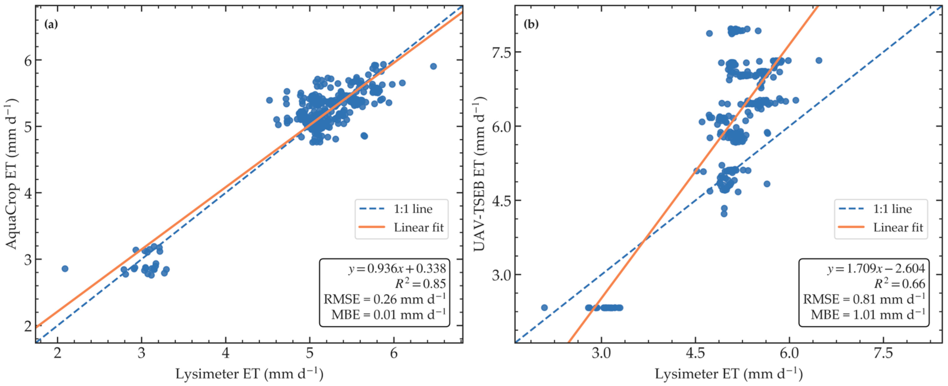
• Direct lysimeter validation (24 drainage lysimeters) confirmed high accuracy of the field-calibrated AquaCrop model (R² = 0.85; RMSE = 0.26 mm d⁻¹; MBE = 0.01 mm d⁻¹) and moderate accuracy of UAV–TSEB (R² = 0.66; RMSE = 0.81 mm d⁻¹; MBE = 1.01 mm d⁻¹) under continuous flooding.
• UAV–TSEB and AquaCrop showed consistent seasonal ET dynamics and robust flux partitioning, with good agreement for total ET (R² = 0.70; RMSE = 1.35 mm d⁻¹), crop transpiration (R² = 0.79; RMSE = 0.99 mm d⁻¹), and soil evaporation (R² = 0.76; RMSE = 1.03 mm d⁻¹).
• A systematic divergence emerged during dense canopy flooded conditions: AquaCrop tended to suppress soil evaporation, whereas UAV–TSEB detected residual evaporation from the flooded surface, highlighting structural differences between daily water-balance and instantaneous energy-balance frameworks.

What are the implications of the main findings?

• The validation framework strengthens confidence in using AquaCrop as a temporally continuous “backbone” and UAV–TSEB as a spatial diagnostic tool, combining daily continuity with spatially explicit ET heterogeneity for field auditing.
• The proposed hybrid approach supports precision irrigation management and WUE-oriented decision making in arid flooded rice systems, by enabling interpretation of productive (T) vs. non-productive (E) water losses and identifying conditions where residual evaporation persists despite canopy closure.

Abstract

Precise estimation of evapotranspiration (ET) is essential for sustainable water management in arid agroecosystems, particularly for high-water-demand crops such as rice. This study integrated very-high-resolution UAV thermal–multispectral imagery with a Two-Source Energy Balance model (UAV–TSEB) and a field-calibrated AquaCrop model to quantify daily ET and its components under continuous flooding on the arid Peruvian coast during the 2024–2025 season. A network of 24 drainage lysimeters provided an independent observational benchmark (ET_lys); to represent the treatment-level response, lysimeter observations were aggregated as the mean across the 24 units for each UAV campaign. Thirteen UAV surveys supplied radiometric surface temperature and biophysical inputs (e.g., NDVI and fractional cover) to derive spatially explicit ET, while AquaCrop provided continuous daily simulations between flight dates. Direct lysimeter-based validation indicated high agreement for AquaCrop (R² = 0.85; RMSE = 0.26 mm d⁻¹; MBE = 0.01 mm d⁻¹) and moderate agreement for UAV–TSEB (R² = 0.66; RMSE = 0.81 mm d⁻¹; MBE = 1.01 mm d⁻¹). Model intercomparison further showed consistent temporal dynamics of ET (R² = 0.70; RMSE = 1.35 mm d⁻¹) and robust partitioning of crop transpiration (R² = 0.79; RMSE = 0.99 mm d⁻¹) and soil evaporation (R² = 0.76; RMSE = 1.03 mm d⁻¹) while revealing a systematic divergence under near-complete canopy cover: AquaCrop tended to suppress evaporation, whereas UAV–TSEB detected residual evaporation from the flooded surface. Overall, the results highlight the complementarity of both approaches—UAV–TSEB as a spatial diagnostic tool and AquaCrop as a temporally continuous simulator—providing a robust framework for ET monitoring, flux partitioning, and water-use-efficiency assessment in water-scarce rice systems.

1. Introduction

The escalating pressure on water resources in intensively irrigated agroecosystems—driven by rising global food demand and drought scenarios exacerbated by climate change—has rendered the precise estimation of evapotranspiration (ET) a critical component for sustainable water management and agricultural productivity [1,2,3,4]. In arid and semi-arid regions such as the Peruvian coast, where water scarcity ranges from medium to high (20–40%) [5], and climatic variability increases evaporative demand [1], there is an urgent need for methodologies capable of quantifying ET at the plot scale with high spatiotemporal resolution [1,2,3,4]. This need is particularly acute for rice, one of the most water-intensive crops on the Peruvian coast (12,000–20,000 m³ ha⁻¹) [1,5], and a key component of irrigated production systems in Lima and Lambayeque [6,7].

ET can be obtained through three main families of approaches, each with complementary strengths and limitations: (i) direct in situ observations (e.g., weighing/drainage lysimeters and eddy covariance), (ii) crop–soil water balance or crop growth models driven by meteorological forcing (e.g., FAO AquaCrop), and (iii) remote-sensing-based retrievals, particularly thermal-infrared (TIR) approaches that infer ET through surface energy balance constraints. Traditional in situ methods (lysimeters, eddy covariance towers) provide high-accuracy measurements but remain constrained by high costs, operational complexity, limited spatial support, and representativeness issues in heterogeneous agricultural fields [8,9,10]. Conversely, process-based models such as AquaCrop (FAO) have proven robust for simulating crop development, water productivity, and ET dynamics at daily time steps, supporting irrigation scheduling and yield assessment [2,11]. However, their 1D, lumped-parameter structure inherently limits the characterization of intra-plot spatial variability, especially under conditions where water depth, canopy structure, and soil surface states vary at short distances [4,6].

Remote sensing provides spatially distributed observations of surface state variables and enables ET retrieval over large areas. Within TIR-based ET retrieval, widely used approaches include: (i) feature-space methods linking LST and vegetation metrics (e.g., Ts–VI “triangle” approaches) that infer evaporative behavior from wet/dry edges [12,13,14], and (ii) surface energy balance models, which can be grouped into single-source and multi-source formulations. Single-source models such as SEBAL [15] and METRIC [16] treat the land surface as a bulk source and have been widely applied to irrigation mapping; however, their single-source assumption can limit explicit representation of soil–canopy exchanges and ET partitioning. Multi-source formulations—particularly the Two-Source Energy Balance model (TSEB)—explicitly separate soil and canopy contributions and enable ET partitioning into evaporation (E) and transpiration (T), which is essential for diagnosing productive versus non-productive water losses and supporting water-use-efficiency (WUE) strategies [17,18,19].

Thermal and multispectral remote sensing from Unmanned Aerial Vehicles (UAVs) has become a robust pathway for field-scale ET mapping because it overcomes key limitations of medium-resolution satellites, providing ultra-high spatial detail and flexible acquisition timing [5,9,20]. UAVs provide direct observations of land surface temperature (LST) that can be rigorously vicariously calibrated and combined with vegetation indices (e.g., NDVI), fractional vegetation cover ($f_c$), and LAI to characterize canopy structure and its control on energy–water exchanges [1,20]. This is especially relevant for continuously flooded rice, where the surface includes both canopy and free-water/soil components and where ET partitioning is central to interpret non-productive evaporation losses. Moreover, UAV products facilitate systematic validation against terrestrial references such as lysimeters and eddy covariance systems [20,21].

Among energy balance models, TSEB has established itself as one of the most physically consistent approaches for ET retrieval because it decouples the radiometric surface temperature ($T_{rad}$) into canopy ($T_c$) and soil ($T_s$) components, enabling independent estimation of transpiration (T) and evaporation (E) [17,18,19,22]. Recent studies have demonstrated the efficacy of the Priestley–Taylor constrained formulation (TSEB-PT) for UAV applications across diverse crops, where sub-field ET partitioning provides actionable insights for irrigation management [2,9,20]. While Ts–VI feature-space methods can be effective for regional monitoring, this study focuses on TSEB because it provides a physically explicit flux partition (E and T) that is particularly valuable in flooded rice water-loss diagnostics and WUE interpretation [17,18,19].

Despite advances in (i) spatially explicit UAV–TSEB retrievals and (ii) temporally continuous crop–water-balance modeling with AquaCrop [23], a key methodological gap remains: few studies have simultaneously integrated vicariously calibrated UAV thermal–multispectral observations with a two-source energy balance model and a process-based crop model, while also benchmarking both modeling pathways against an independent, high-precision lysimeter network within the same experimental unit. This gap is particularly important in flooded rice, where residual evaporation from free-water surfaces may persist even near canopy closure, and where partitioning differences between physically explicit energy-balance residuals and conceptual canopy-limited evaporation schemes can become critical for interpretation and management.

Therefore, this study aims to quantify daily evapotranspiration and its components in continuously flooded rice at the Irrigation Experimental Area (AER) of the Universidad Nacional Agraria La Molina (UNALM, Peru), integrating three complementary elements: (i) UAV-based thermal–multispectral retrievals coupled to TSEB for spatially explicit ET and flux partitioning, (ii) a locally calibrated AquaCrop model for temporally continuous daily simulations of ET and crop dynamics, and (iii) a network of 24 drainage lysimeters providing an independent observational benchmark for direct validation. Importantly, both AquaCrop and UAV–TSEB are evaluated against ET_lys to establish an explicit validation hierarchy. We hypothesize that: (1) UAV–TSEB will resolve within-treatment spatial variability and provide physically consistent E–T partitioning at sub-field scale, (2) AquaCrop will provide stable daily continuity between UAV acquisitions and accurately represent treatment-mean ET dynamics, and (3) the combined framework will reduce uncertainty and improve interpretability for precision irrigation and WUE assessment in water-scarce rice systems.

2. Materials and Methods

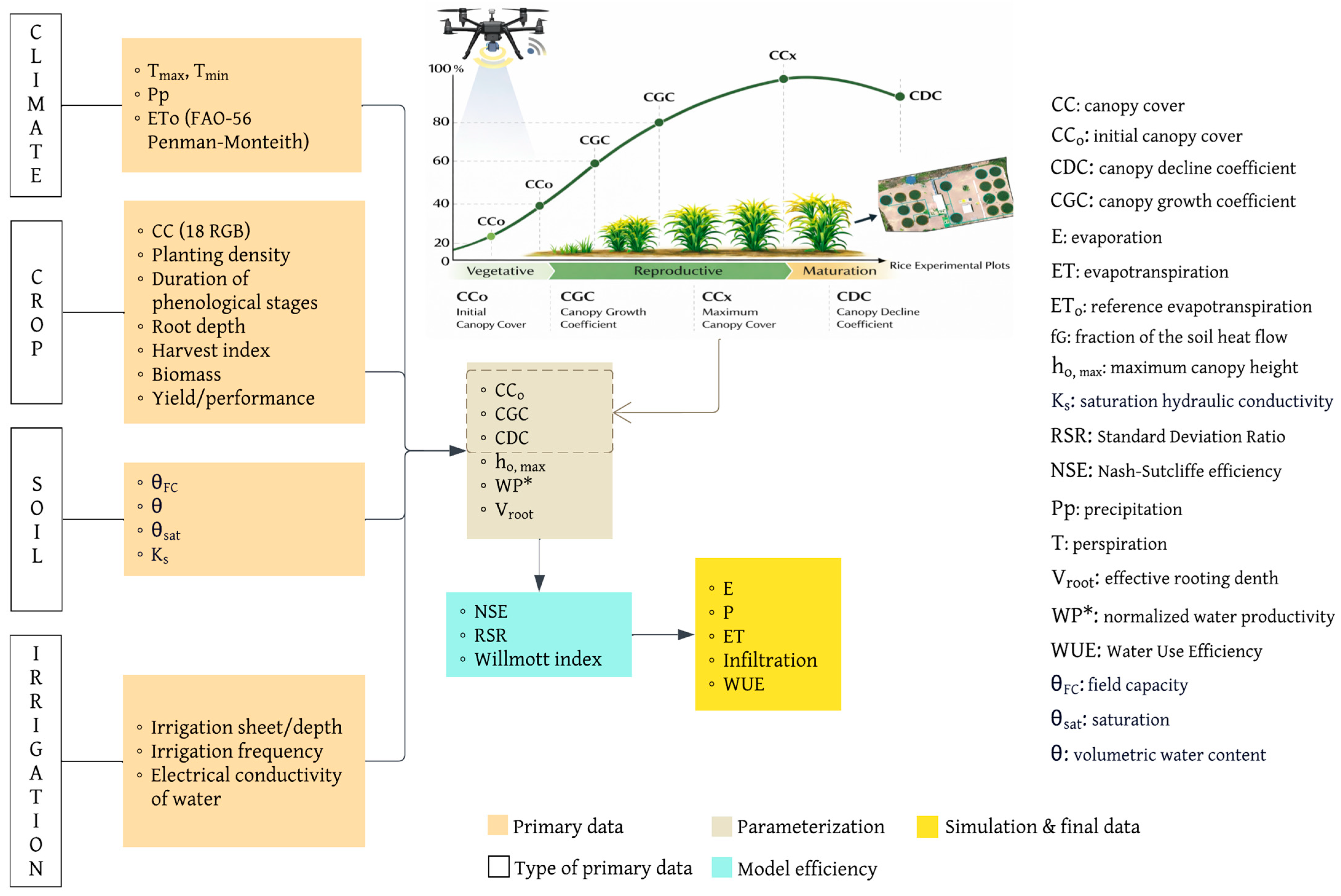
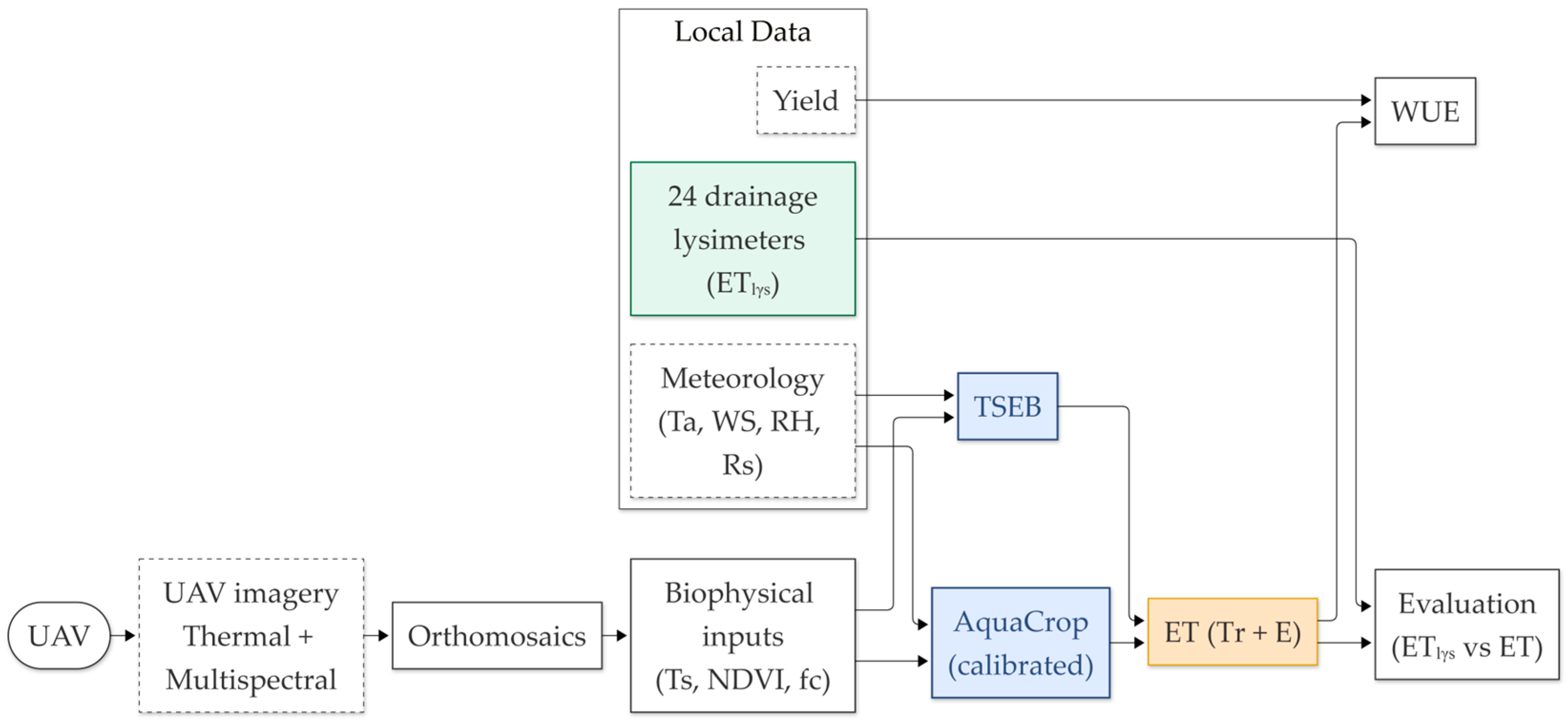
Figure 1 outlines the end-to-end methodological framework implemented during the 2024–2025 rice growing season on the arid Peruvian coast. The workflow integrates high-resolution UAV thermal–multispectral observations with local forcing and reference measurements to produce spatially explicit evapotranspiration and water productivity estimates. First, UAV imagery is processed into orthomosaics and biophysical inputs (e.g., radiometric surface temperature $T_s$, NDVI, and fractional cover $f_c$). These products, together with meteorological forcing (air temperature, wind speed, relative humidity, and incoming solar radiation), drive the two-source energy balance model (TSEB) to retrieve instantaneous ET and partition it into transpiration ($T_r$) and evaporation ($E$). In parallel, AquaCrop is calibrated and run to provide continuous daily simulations of ET and yield. Finally, model outputs are evaluated against the drainage-lysimeter network (ET_lys), and the resulting ET estimates are combined with observed yield to compute water use efficiency (WUE).

2.1. Study Area

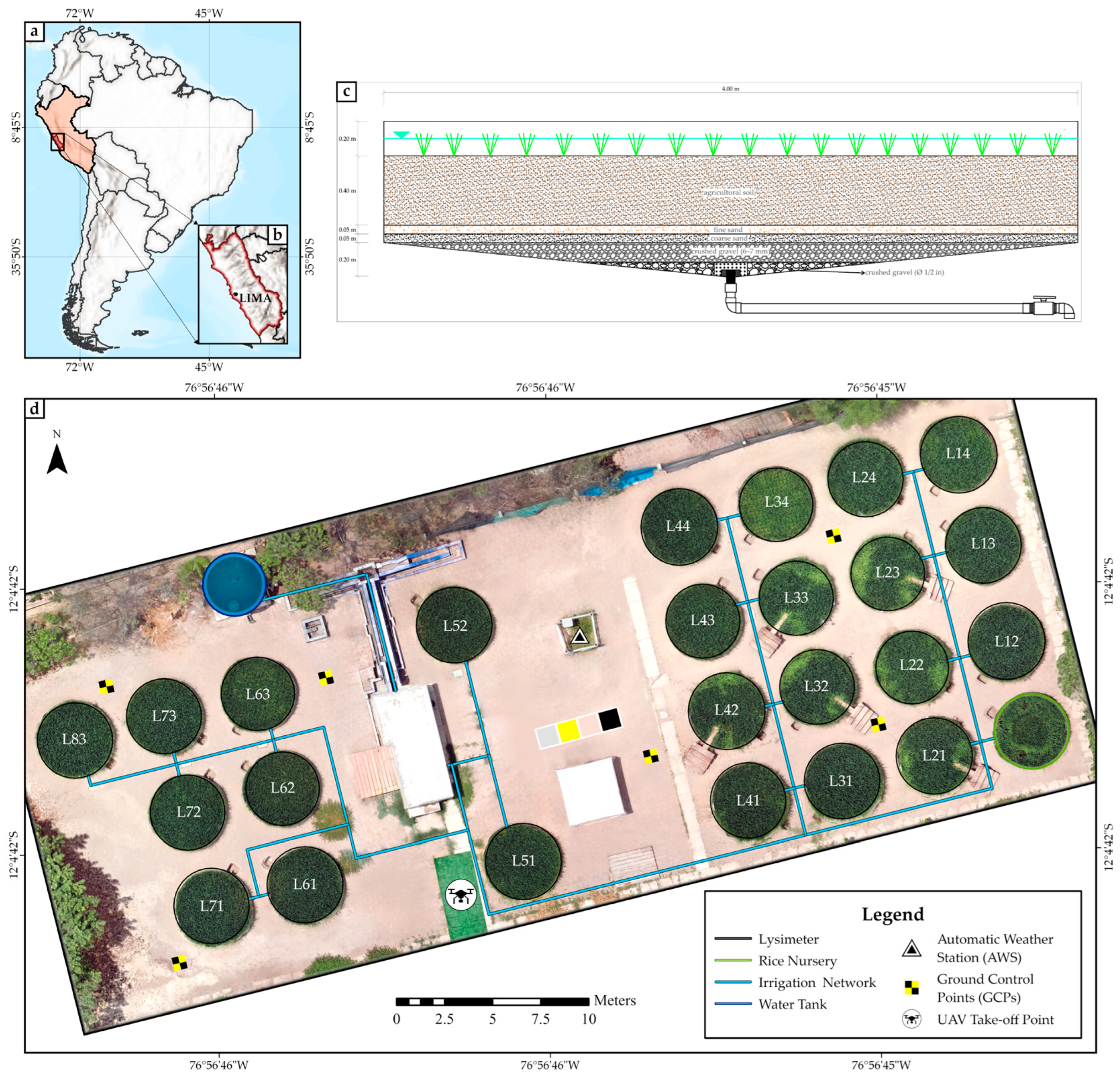
The study was conducted at the Irrigation Experimental Area (AER) of the Universidad Nacional Agraria La Molina (UNALM), located on the central coast of Peru (La Molina district, Lima), at coordinates 12°04′42″ S and 76°56′46″ W, with an altitude of approximately 240 m a.s.l. (Figure 2a,b). The region exhibits an arid subtropical climate, characterized by annual precipitation typically less than 10 mm, high atmospheric stability, and marked seasonality in relative humidity. These stable atmospheric conditions are highly favorable for evapotranspiration experiments under controlled irrigation management. The general layout of the experimental site within the hydraulic network is illustrated in Figure 2d, while the specific lysimeter design is detailed in Figure 2c.

Meteorological Conditions

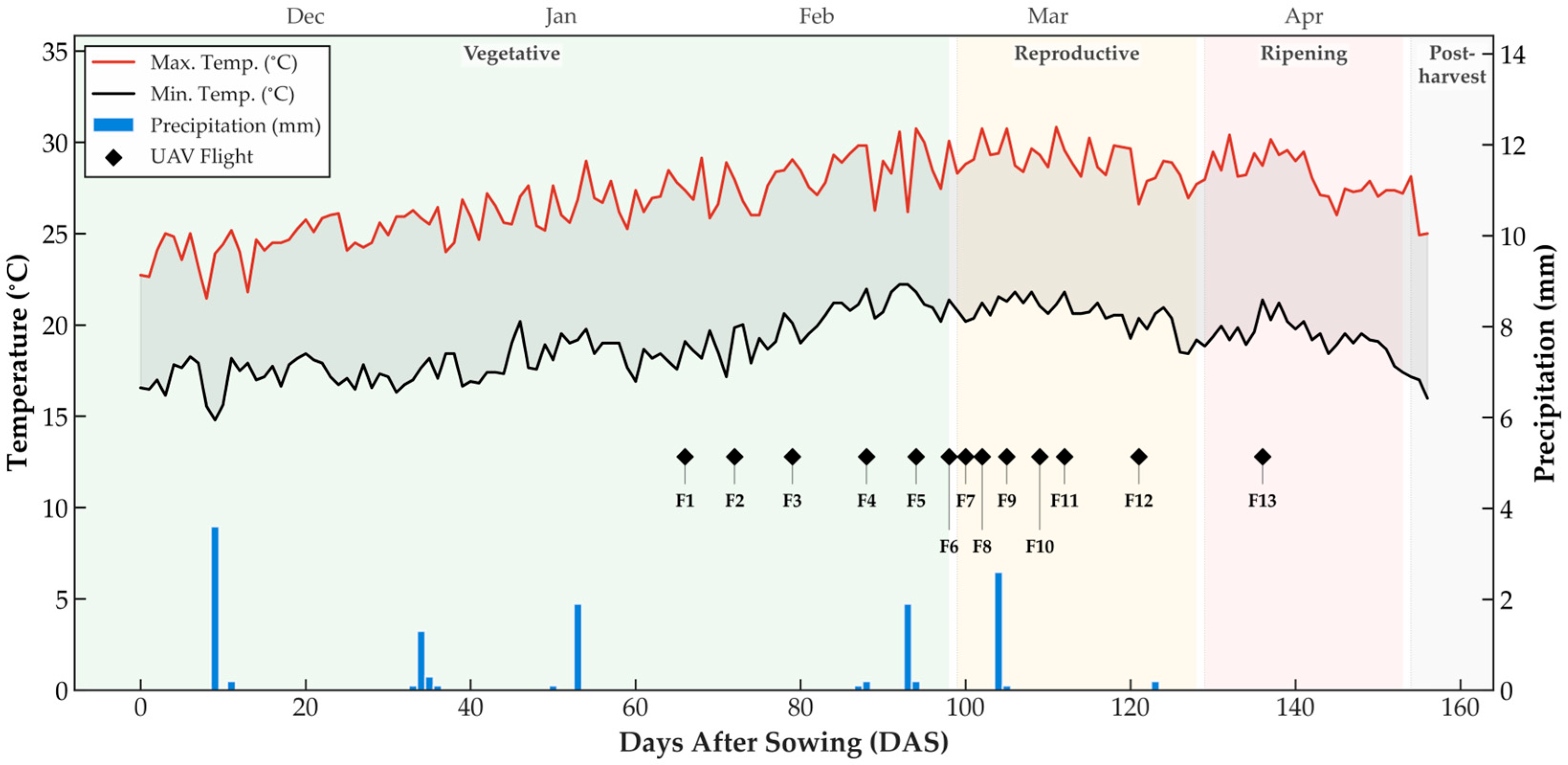
Meteorological variables required for evapotranspiration modeling were recorded using a portable automatic weather station (ATMOS 41, METER Group, Pullman, WA, USA) coupled to a ZL6 data logger. The station was installed at 2 m above ground level and centrally located within the AER–UNALM to represent the micrometeorological conditions of the experiment. Air temperature, relative humidity, wind speed, incoming solar radiation, and precipitation were continuously recorded and used as atmospheric forcing for the TSEB model and as climatic inputs for AquaCrop simulations. Based on these time series, intra-seasonal variability was characterized, and daily and monthly aggregates were derived to support the analysis of seasonal atmospheric demand and its relationship with evapotranspiration dynamics (Figure 3).

2.2. Soil and Irrigation Water Characterization

Soil physical and hydraulic properties were determined to parameterize the AquaCrop model and interpret thermal dynamics. The soil texture was classified as sandy clay loam (54% sand, 19% silt, and 27% clay), characterized by a bulk density of 1.41 $\mathrm{g} \mathrm{c}{\mathrm{m}}^{-3}$ and a total porosity of 47.2%. Regarding soil water retention, the volumetric water content at Field Capacity (${\theta }_{FC}$) and Permanent Wilting Point (${\theta }_{PWP}$) were 0.2976 $\mathrm{c}{\mathrm{m}}^3 \mathrm{c}{\mathrm{m}}^{-3}$ and 0.1627 $\mathrm{c}{\mathrm{m}}^3 \mathrm{c}{\mathrm{m}}^{-3}$, respectively. The soil presented a moderate organic matter content (4.32%) and an electrical conductivity (EC) of 5.17 $\mathrm{d}\mathrm{S} {\mathrm{m}}^{-1}$, indicating moderately saline conditions but without sodium hazards (SAR = 0.08).

Irrigation was supplied from the local pressurized network with water classified as ${\mathrm{C}}_2-{\mathrm{S}}_1$ (medium salinity, low sodium), having a pH of 6.95 and an EC of 0.47 $\mathrm{d}\mathrm{S} {\mathrm{m}}^{-1}$. This quality was suitable for the experimental trials, posing no chemical restrictions for crop development or evapotranspiration assessment. A detailed physicochemical characterization of the soil and water resources is provided in Table S1 (Supplementary Material).

2.3. Experimental Design and Crop Management

The experimental infrastructure consisted of a network of 24 drainage lysimeters (Figure 2d). Each lysimeter was a circular reinforced-concrete unit with a 4.0 m internal diameter and an effective profile depth of ~0.70 m (substrate + soil layers), designed to enable controlled ponding and precise drainage collection. As detailed in the cross-sectional profile (Figure 2c), the lysimeters featured a stratified substrate system comprising a 0.20 m basal layer of crushed gravel (Ø 6–7 mm) to promote gravitational drainage towards a central outlet valve, followed by two 0.05 m filtering layers of coarse and fine sand, and capped with a 0.40 m top layer of reconstituted agricultural soil adjusted to match the local field bulk density.

The INIA 515-Capoteña rice variety was planted on 11 November 2024, using the nursery technique. Seedlings were transplanted 33 days after sowing (DAS) with a spacing of 0.20 m × 0.20 m (two seedlings per hill). This specific planting density was selected to promote rapid and homogeneous canopy closure, ensuring a robust parameterization of the fractional vegetation cover ($fc$). This parameter is critical for both the flux partitioning (soil vs. canopy) in the Two-Source Energy Balance (TSEB) model and the biomass engine in AquaCrop.

The 24 lysimeters were managed under a uniform Continuous Flooding (CF) irrigation regime throughout the entire phenological cycle. Water supply was provided by the AER-UNALM hydraulic infrastructure, fed by the Rímac and Chillón river basins, and distributed via a pressurized automated network. Prior to establishment, laser land leveling was performed. This practice was decisive for minimizing spatial gradients in water depth and soil moisture, thereby guaranteeing the surface uniformity and radiometric consistency required for the accurate interpretation of spatial evapotranspiration (ET) variability.

Fertilization followed a dose of 250–106–60 (N–P–K) using urea, diammonium phosphate, and potassium sulfate. Phosphorus and potassium (100%), along with 30% of nitrogen, were applied at transplanting. The remaining nitrogen was fractionated across key phenological stages—tillering, panicle initiation, and flowering—following the protocol described by Heros et al. [24]. This strategy ensured stable growth and minimized energy flux biases associated with nutritional deficiencies.

Phenological evolution was monitored through the accumulation of Growing Degree Days (GDD) with a base temperature ($T_{base}$) of 10 °C. This bioclimatic approach enabled the synchronization of flight campaigns with the physiological stages that dictate water consumption [23]. In total, 13 UAV data acquisition campaigns were executed, strategically distributed across the vegetative, reproductive, and ripening phases to capture the complete temporal dynamics for model validation (

Table 1. Schedule of UAV flight campaigns, days after sowing (DAS), and corresponding crop phenological stages.

Flight	DAS	Phenology
F1	66	Vegetative
F2	72	Vegetative
F3	79	Vegetative
F4	88	Vegetative
F5	94	Vegetative
F6	98	Vegetative
F7	100	Reproductive
F8	102	Reproductive
F9	105	Reproductive
F10	109	Reproductive
F11	112	Reproductive
F12	121	Reproductive
F13	136	Ripening

).

2.4. UAV Data Acquisition and Orthomosaic Processing

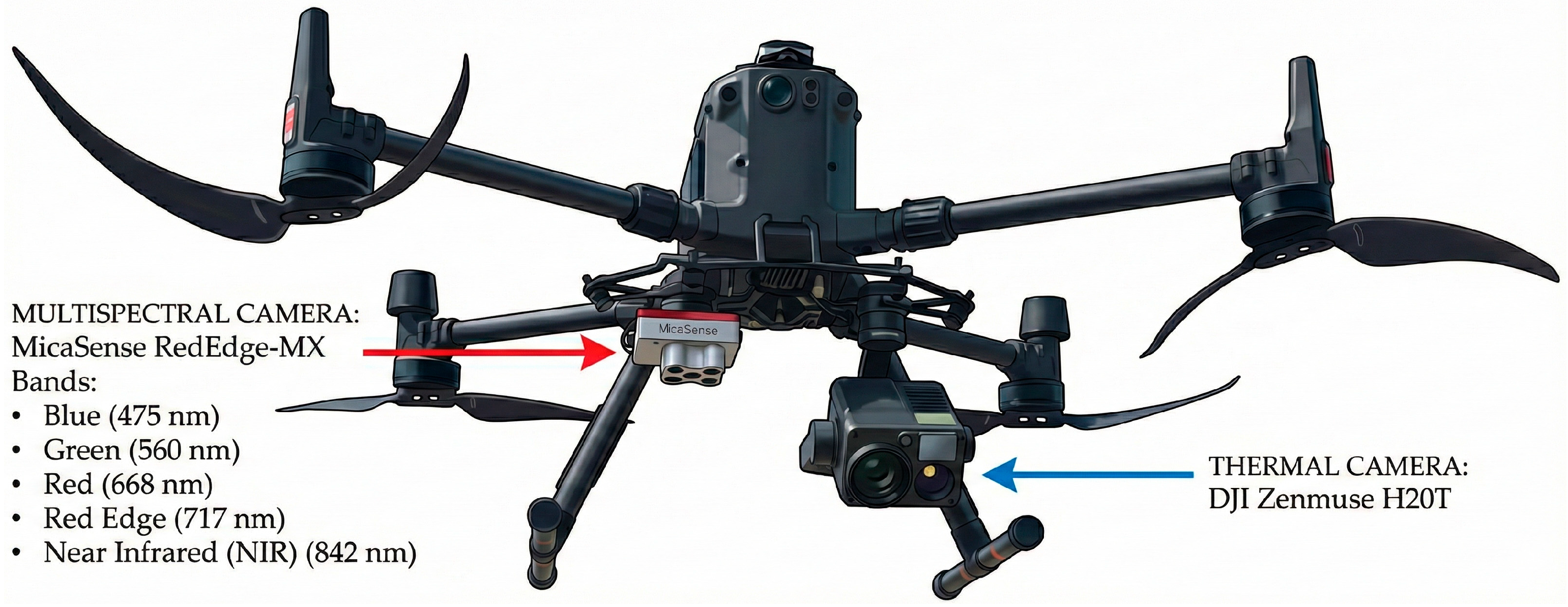
Remote sensing data were acquired using a quadcopter platform (Matrice 300 RTK, DJI, Shenzhen, China) equipped with a dual-sensor payload configuration. This payload included a multispectral camera (RedEdge-MX, MicaSense, Seattle, WA, USA) capturing five discrete spectral bands (Blue, Green, Red, Red Edge, and Near-Infrared) and a hybrid sensor (Zenmuse H20T, DJI) for simultaneous radiometric thermal and high-resolution RGB imaging (Figure 4). Flight campaigns were conducted under clear-sky conditions and strictly synchronized within a ±1-h window of solar noon to minimize shadowing effects and ensure maximum solar irradiance stability. The flight altitude was set at 25 m above ground level (AGL) with a frontal and side overlap of 80%. This low-altitude configuration was selected to achieve ultra-high spatial resolution, yielding native Ground Sampling Distances (GSD) of approximately 0.8 cm pixel⁻¹ for RGB imagery (H20T)—utilized for precise vegetation masking and canopy cover (CC) classification—and 1.6 cm pixel⁻¹ for both the multispectral (RedEdge-MX) and thermal (H20T) datasets.

Photogrammetric processing was performed in Pix4Dmapper Pro (Pix4D S.A., Prilly, Switzerland), where geometric accuracy was ensured using the platform’s RTK positioning corrected via a D-RTK 2 Mobile Station and validated with Ground Control Points (GCPs). Regarding radiometric consistency, multispectral images were calibrated using a Calibrated Reflectance Panel (CRP) captured immediately before and after each flight to convert digital numbers (DN) into surface reflectance values. For the thermal data, a rigorous vicarious calibration protocol was applied to correct Land Surface Temperature (LST) retrievals; following Ramos-Fernández et al. [5], handheld infrared radiometers were used to measure the kinetic temperature of four distinct reference targets (yellow fabric, bare soil, black fabric, and aluminum foil) simultaneously with the UAV overpass, establishing a linear regression model (R² > 0.95) for each flight date to correct atmospheric attenuation and sensor bias.

Finally, to ensure spatial consistency for the Two-Source Energy Balance (TSEB) modeling, all resulting orthomosaics were spatially aggregated (resampled) to a common resolution of 0.15 m. This target resolution was strategically selected considering the dimensions of the experimental units (24 lysimeters with a 4 m diameter), ensuring that each lysimeter integrated several hundred thermal pixels to guarantee adequate spatial support for the estimation and validation of daily evapotranspiration. This resampling step minimizes micro-scale noise associated with complex canopy geometry and ensures precise geometric co-registration between thermal inputs (Ts) and multispectral variables (NDVI, fc, LAI) required for the model parametrization.

2.5. Retrieval of Biophysical and Thermal Variables

Vegetation indices and biophysical parameters were derived from the radiometrically calibrated multispectral orthomosaics. The Normalized Difference Vegetation Index (NDVI), utilized as a proxy for canopy vigor and fractional cover, was calculated as:

$$\mathrm{NDVI} = {\displaystyle \frac{\mathrm{NIR}-\mathrm{RED}}{\mathrm{NIR} + \mathrm{RED}}}$$

(1)

where NIR and Red represent surface reflectance in the near-infrared and red bands, respectively. Leaf Area Index (LAI) and fractional vegetation cover ($fc$) were spatially estimated based on site-specific empirical relationships established between UAV-derived NDVI and in situ measurements. This calibration followed the semi-empirical approach validated for rice crops in the La Molina region [1]. The specific regression models and their statistical validation are detailed in Section 3.2.

Surface albedo (α) was computed using a weighted integration of the multispectral bands, consistent with narrow-to-broadband conversion formulations used in previous studies [8,25]. Regarding thermal variables, radiometric surface temperature ($T_{rad}$) was retrieved from the thermal orthomosaics. To minimize instrumental bias and atmospheric effects, $T_{rad}$ was adjusted using the linear regression models derived from the vicarious calibration targets described in Section 2.4, aligning with calibration procedures for UAV campaigns [7].

2.6. TSEB Modeling and Energy Flux Partitioning

2.6.1. Two-Source Energy Balance (TSEB) Model Formulation

Evapotranspiration (ET) was estimated for the 13 acquisition dates using the Two-Source Energy Balance (TSEB) model, originally developed by Norman et al. [17] and subsequently refined by Kustas et al. [18]. In contrast to single-source approaches, TSEB theoretically decouples surface energy fluxes into two nominal components—soil and canopy—allowing for the independent estimation of soil evaporation ($E$) and crop transpiration ($T$).

The model was designed to improve the accuracy of Latent Heat Flux ($LE$) estimation over heterogeneous agricultural landscapes [17,26]. In this study, the TSEB-PT approach was applied, which incorporates the Priestley et al. [27] assumption to constrain the initial canopy transpiration. This formulation enables a physical partitioning of the surface energy balance, separating Sensible Heat ($H$) and Latent Heat ($LE$) fluxes. Several studies have demonstrated the efficacy of TSEB in complex agricultural environments, yielding flux estimates comparable to eddy covariance system measurements [28,29].

The core of the model decomposes the directional radiometric surface temperature $T_{rad}$($\theta$) into soil kinetic temperature ($T_s$) and canopy kinetic temperature ($T_c$), weighted by the fractional vegetation cover visible to the sensor, $fc \left(\theta \right)$:

$$T_{rad}(\theta ) \approx {\left[f_c\left(\theta \right)·T_c^4+\left(1-f_c\left(\theta \right)\right)·T_s^4\right]}^{{\displaystyle \frac{1}{4}}}$$

(2)

The total Net Radiation ($R_n$) is expressed as the sum of the soil ($R_{ns}$) and canopy ($R_{nc}$) components [30,31]:

$$R_n=R_{ns}+R_{nc}$$

(3)

The net radiation for each component is calculated by considering the canopy transmission of longwave (${\tau }_l$) and shortwave (${\tau }_S$) radiation, incoming longwave ($L_d$) and shortwave ($S_d$) radiation, emissivity ($ϵ$), albedo ($\alpha$), and surface temperatures [31,32].

Note: The soil equation explicitly incorporates energy loss via thermal emission ($-{ϵ}_s\sigma T_s^4$).

$$R_{ns}={{\tau }_{l}L}_d+\left(1-{\tau }_l\right){\epsilon }_c\sigma T_s^4+{\tau }_s\left(1-{\alpha }_s\right)S_d$$

(4)

$$R_{nc}=\left(1-{\tau }_l\right)\left(L_d+{\epsilon }_s\sigma T_s^4-2{\epsilon }_c\sigma T_c^4\right)+\left(1-{\tau }_s\right)\left(1-{\alpha }_c\right)S_d$$

(5)

where $\sigma$ is the Stefan–Boltzmann constant. The system energy fluxes are solved via the balance equations:

$$R_{ns}=H_s+{LE}_s+G$$

(6)

$$R_{nc}=H_c+{LE}_c$$

(7)

where G represents the soil heat flux, estimated as a fraction of $R_{ns}$. The sensible heat fluxes for the soil $\left(H_s\right)$ and canopy ($H_c$) are calculated theoretically based on the series resistance network [17,33,34]:

$$H_s={\rho C}_p{\displaystyle \frac{T_s-T_{ac}}{R_s}}; H_c={\rho C}_p{\displaystyle \frac{T_c-T_{ac}}{R_x}}$$

(8)

where $\rho$ is the air density, $C_p$ is the specific heat of air, $T_{ac}$ is the air temperature within the canopy interspace, $R_s$ is the aerodynamic resistance above the soil surface, and $R_x$ is the total boundary layer resistance of the canopy leaves.

2.6.2. Model Implementation and Data Processing Workflow

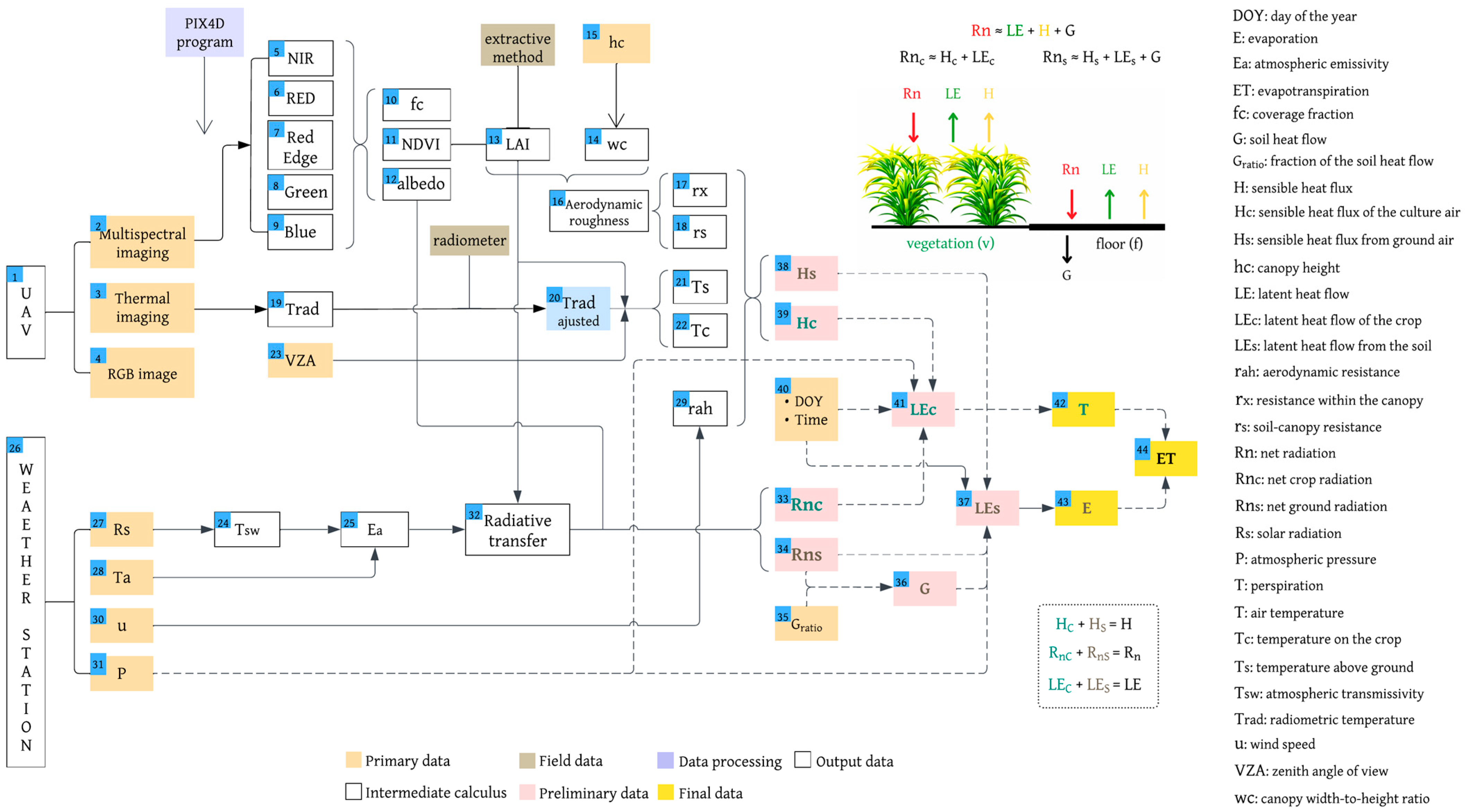
The TSEB model was implemented in Python using the open-source pyTSEB library (version v2.3) (https://github.com/hectornieto/pyTSEB, accessed on 20 January 2025). Figure 5 summarizes the end-to-end workflow, integrating UAV-derived thermal–multispectral products, field biophysical measurements, and meteorological forcing to retrieve instantaneous energy fluxes and derive daily evapotranspiration.

The processing chain commences with the UAV platform (1) acquiring three primary datasets: multispectral (2), thermal (3), and RGB imagery (4). From the multispectral bands (5–9), the vegetation cover fraction, $fc$ (10), NDVI (11), and surface albedo (12) were calculated, allowing for the characterization of canopy structure and condition. These layers were integrated with field measurements—specifically Leaf Area Index, LAI (13), canopy width-to-height ratio, $Wc$ (14), and canopy height, $hc$ (15)—to parameterize the aerodynamic roughness (16) and the internal resistance network, comprising the canopy boundary layer resistance, $r_x$ (17), and the soil aerodynamic resistance, $r_s$ (18).

Simultaneously, the raw radiometric temperature, $T_{rad}$ (19), was retrieved from the thermal imagery and rigorously corrected using vicarious calibration targets to obtain the adjusted $T_{rad}$ (20). This variable, combined with the View Zenith Angle, VZA (23), drove the decomposition of the directional temperature into soil kinetic temperature, $T_s$ (21), and canopy kinetic temperature, $T_c$ (22).

Meteorological forcing variables registered by the Automatic Weather Station (26)—including $R_s$ (27) $T_a$ (28), $u$ (30), and $P$ (31) —were utilized to calculate the aerodynamic resistance to heat transport, $r_{ah}$ (29), and atmospheric emissivity, ${\epsilon }_a$ (23). Using a radiative transfer scheme (32), the total net radiation was partitioned into net canopy radiation, $R_{n,c}$ (33), and net ground radiation, $R_{n,s}$ (34).

The energy balance was solved iteratively. The soil heat flux, $\mathrm{G}$ (36), was estimated as a fraction of $R_{n,s}$ (34). Sensible heat fluxes for soil, $H_s$ (38), and canopy, $H_c$ (39), were calculated based on thermal gradients. The canopy latent heat flux, ${LE}_c$ (41), was initialized using the Priestley-Taylor approximation considering the DOY and time (40), while the soil latent heat flux, ${LE}_s$ (37), was solved as a residual. This allowed for the derivation of instantaneous crop transpiration, $T$ (42), soil evaporation, $E$ (43), and total evapotranspiration, $ET$ (44).

Finally, instantaneous UAV–TSEB fluxes were converted to daily evapotranspiration using incoming solar radiation scaling rather than assuming a constant evaporative fraction. Specifically, the daily ET was obtained by scaling the instantaneous ET using the ratio between daily integrated and overpass-time incoming solar radiation, following the one-time-of-day upscaling approach commonly adopted for remote-sensing ET applications. This strategy is more robust for arid coastal conditions where advective effects can violate the constancy of evaporative fraction, and it enables consistent daily comparisons with AquaCrop simulations.

2.6.3. Temporal Upscaling to Daily ET (Radiation-Scaling Method)

To enable direct comparison with daily lysimeter evapotranspiration (ET_lys) and the daily AquaCrop outputs, instantaneous UAV–TSEB latent heat fluxes retrieved at the flight time were upscaled to daily evapotranspiration (ET_d). Although daily integration is often performed using a constant evaporative fraction (EF) assumption, this approach can be sensitive under advective conditions and during periods of strong afternoon atmospheric coupling. Therefore, in this study we did not apply constant-EF scaling. Instead, we adopted the incoming solar radiation scaling method originally proposed by Jackson et al. [35] and further evaluated for remote-sensing applications, which assumes that, under clear-sky and radiatively driven conditions, the diurnal course of ET is primarily controlled by the available radiative energy. Daily ET was computed as [36]:

$${ET}_d={ET}_{inst}{\displaystyle \frac{R_{s,d}}{R_{s, inst}}}$$

(9)

where $E{T}_{inst}$ is the instantaneous evapotranspiration estimated by UAV–TSEB at the overpass time (mm $h^{-1}$ or equivalent after unit conversion), $R_{s,inst}$ is the incoming shortwave radiation measured at the flight time (W m⁻²), and $R_{s,d}$ is the daily integrated incoming shortwave radiation derived from the on-site automatic weather station (MJ ${\mathrm{m}}^{-2}$ ${\mathrm{d}}^{-1}$). UAV surveys were conducted within a ±1 h window around solar noon under predominantly clear-sky conditions, which supports the applicability of radiation-based scaling and reduces the sensitivity to late-afternoon advection relative to EF-based methods.

2.7. AquaCrop Setup and Field Calibration

Crop water productivity and biomass accumulation were simulated using the FAO AquaCrop model (Version 7.1). This process-based model was selected for its robustness in simulating the yield response to water and its ability to distinguish between soil evaporation ($E$) and crop transpiration ($T$) under varying irrigation management strategies [23,37]. The comprehensive modeling workflow, illustrating the integration of input data, parameterization, and the calibration loop, is presented in Figure 6.

The model initialization required the integration of four primary data modules: Climate, Soil, Crop, and Irrigation. The simulation was driven by daily meteorological records ($T_{max}$, $T_{min}$, $P$) acquired from the on-site AWS, while reference evapotranspiration (${ET}_o$) was computed externally using the FAO-56 Penman-Monteith method. The soil module was parameterized using the specific hydraulic properties determined in Section 2.2, including volumetric water content at saturation $\left({\theta }_{sat}\right)$, field capacity $\left({\theta }_{FC}\right)$, and permanent wilting point $\left({\theta }_{PWP}\right)$, along with the saturated hydraulic conductivity ($K_s$), following parameterization schemes for loamy soils. Crop physiological parameters were adjusted to reflect local rice cultivar characteristics—such as planting density, harvest index, and maximum rooting depth—while the management module was set to a Continuous Flooding (CF) regime to mirror the experimental conditions [38,39,40,41].

To ensure high-fidelity simulations, a site-specific calibration strategy was implemented. Unlike standard calibrations relying solely on final yield, this study utilized UAV-derived high-resolution RGB imagery as a temporal constraint for canopy development. The observed Green Canopy Cover ($CC$) values were used to iteratively tune the conservative growth parameters, specifically the Canopy Growth Coefficient (CGC) for the expansion phase and the Canopy Decline Coefficient (CDC) for the senescence phase. This calibration ensured that the simulated canopy curve matched the observed phenological progression, thereby reducing uncertainty in the transpiration ($T$) estimation. The statistical validation of this canopy development simulation, including metrics such as the Nash-Sutcliffe Efficiency (NSE) and the Willmott Index of Agreement (d), is detailed in Section 3.2.

2.8. Model Evaluation and Statistical Analysis

2.8.1. Lysimeter-Derived ET_lys Computation

Daily evapotranspiration observed by the drainage lysimeter network (ET_lys) was used as the independent reference dataset for model evaluation. For each lysimeter, ET_lys was computed using a daily water-balance approach:

$${\mathrm{ET}}_{\mathrm{lys}} = \mathrm{I} + \mathrm{P}-\mathrm{D}-∆\mathrm{S}$$

(10)

where $I$ is applied irrigation (mm), $P$ is precipitation (mm), $D$ is measured drainage (mm), and $\Delta S$ is the change in water storage within the soil–water system (mm) between consecutive days. Irrigation and drainage were expressed as equivalent water depth (mm) over the lysimeter area, and precipitation was obtained from the on-site automatic weather station. Under continuous flooding (CF), $\Delta S$ accounts for day-to-day changes in ponded water depth and soil-water storage; thus, ET_lys represents the integrated evapotranspiration response of the flooded rice system at the lysimeter scale.

To represent the treatment-level response under the uniform CF management and to ensure scale consistency with model outputs, lysimeter observations were aggregated as the mean across the 24 units for each day and for each UAV acquisition date.

2.8.2. Direct Validation: ET_lys vs. AquaCrop and ET_lys vs. UAV–TSEB

Model performance was quantified through direct comparisons against the observational benchmark ET_lys. AquaCrop daily evapotranspiration was validated against ET_lys over the full study period, leveraging the model’s daily continuity. UAV–TSEB daily evapotranspiration was validated against ET_lys for the UAV monitoring dates, after temporally upscaling instantaneous energy-balance fluxes to daily ET. For both validations, agreement was assessed using standard goodness-of-fit and error metrics, including the coefficient of determination (R²), root mean square error (RMSE), and mean bias error (MBE), computed as:

$${\mathrm{R}}^2 = 1-{\displaystyle \frac{{\sum }_{\mathrm{j}=1}^{\mathrm{n}}{({\mathrm{Y}}_{\mathrm{j}}-{\widehat{\mathrm{Y}}}_{\mathrm{j}})}^2}{{\sum }_{\mathrm{j}=1}^{\mathrm{n}}{({\mathrm{Y}}_{\mathrm{j}}-\stackrel{\mathrm{-}}{\mathrm{Y}})}^2}}$$

(11)

$$\mathrm{RMSE}=\sqrt{{\displaystyle \frac{{\sum }_{\mathrm{j}=1}^{\mathrm{n}}{\left({\mathrm{Y}}_{\mathrm{j}}-{\widehat{\mathrm{Y}}}_{\mathrm{j}}\right)}^2}{\mathrm{n}}}}$$

(12)

$$\mathrm{MBE}={\displaystyle \frac{1}{\mathrm{n}}}\sum _{\mathrm{i}=1}^{\mathrm{n}}({\mathrm{P}}_{\mathrm{i}}-{\mathrm{O}}_{\mathrm{i}})$$

(13)

2.8.3. Intercomparison: UAV–TSEB vs. AquaCrop (ET and Flux Partitioning)

In addition to the direct lysimeter-based validation, a complementary intercomparison between UAV–TSEB and AquaCrop was conducted to interpret methodological differences between an instantaneous energy-balance approach and a daily crop water-balance model under continuous flooding. This analysis evaluated total daily evapotranspiration (ET_d) and the partitioned components of transpiration (T_c) and soil evaporation (E) at the UAV acquisition dates, and results were stratified by phenological stage (vegetative, reproductive, and ripening) to identify potential stage-dependent behavior. Importantly, this intercomparison was used to support process interpretation of ET partitioning and temporal scaling, whereas ET_lys remained the primary reference dataset for model validation.

3. Results

3.1. Meteorological Conditions and UAV Acquisition Stability

The precision of energy flux modeling intrinsically relies on atmospheric stability during radiometric acquisition. Figure S1 (Supplementary Material) details the high-frequency dynamics of the meteorological forcing variables recorded during the 13 flight campaigns.

As depicted in the shaded flight window of Figure S1, data acquisitions were strategically synchronized with solar noon, covering a temporal window where incident solar radiation ($R_s$) reached average maximum values of $840.5\pm 209.5 \mathrm{W} {\mathrm{m}}^{-2}$ (Figure S1a). This synchronization ensured that the captured radiometric temperature ($T_{rad}$) represented the peak daily evaporative demand. Furthermore, wind conditions remained stable and low ($\mathrm{u}<2.0 \mathrm{m} {\mathrm{s}}^{-1}$) during the flights (Figure S1d), which is critical for minimizing advection errors and validating the surface boundary layer equilibrium assumption required by the TSEB model. Table S2 summarizes the specific micrometeorological conditions for each flight date.

3.2. Validation of Biophysical Constraints: LAI and Canopy Cover

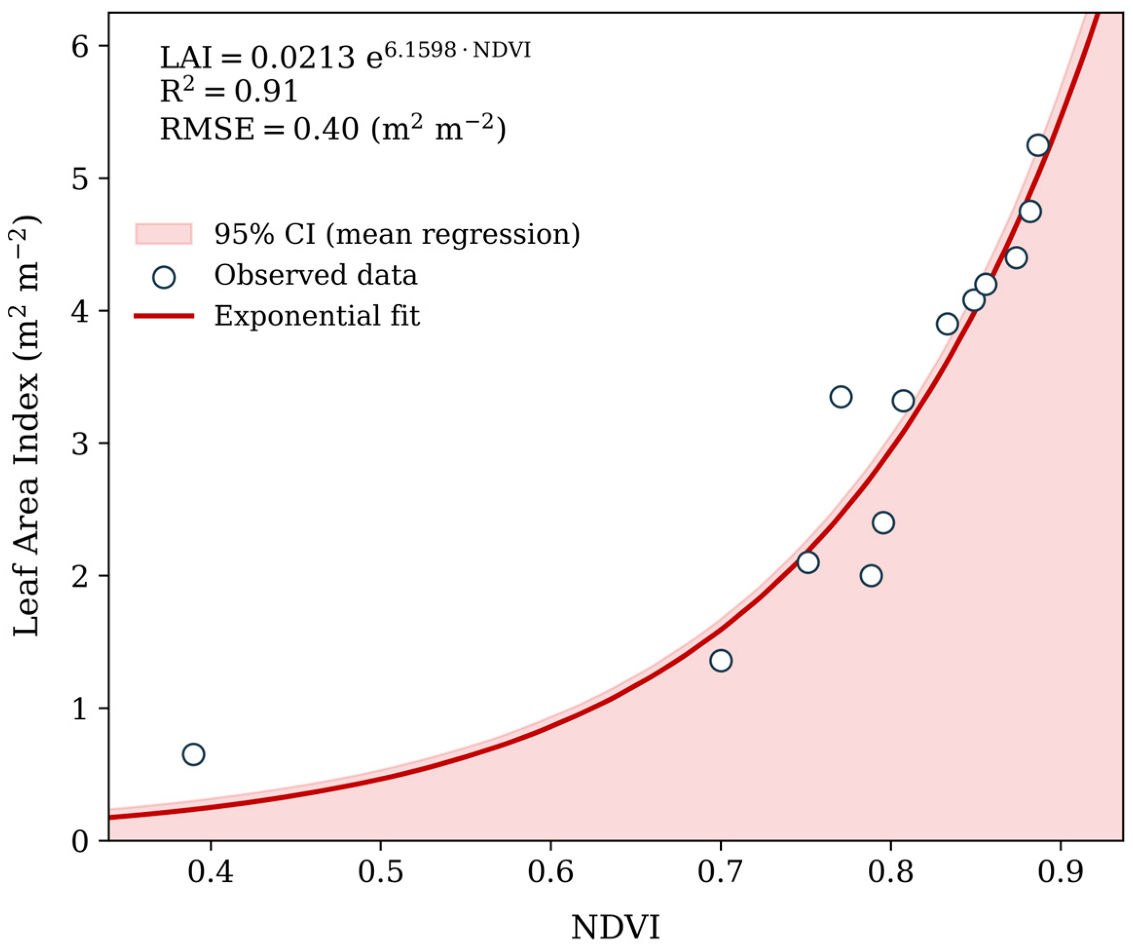
Accurate estimation of canopy structure is a prerequisite for both flux partitioning (TSEB) and biomass simulation (AquaCrop). The empirical relationship developed to estimate Leaf Area Index (LAI) from UAV-derived NDVI is presented in Figure 7. This relationship was obtained by correlating LAI (estimated via the extractive method) with co-located NDVI measurements acquired on multiple dates throughout crop development, enabling the retrieval of spatial LAI variability from the multispectral orthomosaics.

To determine the optimal functional form of this relationship, the dataset was analyzed using Eureqa (version 1.24.0) (Nutonian, Inc., Boston, MA, USA), a symbolic regression software based on evolutionary algorithms. Unlike traditional regression methods that fit parameters to a pre-defined equation, this approach identifies both the mathematical structure and the model parameters simultaneously, without imposing a priori assumptions [42]. The analysis identified an exponential function as the most robust predictor, yielding the following equation:

$$\mathrm{LAI} = 0.0213{\mathrm{e}}^{6.1598\times \mathrm{NDVI}}$$

(14)

The model exhibited a strong statistical performance (R² = 0.91) and low error (RMSE = 0.40 m² m⁻²), supporting its suitability to characterize LAI dynamics over the observed canopy development range. In Figure 7, the shaded envelope represents the 95% confidence interval of the mean regression (i.e., uncertainty in the fitted relationship), rather than a 95% prediction interval for individual observations.

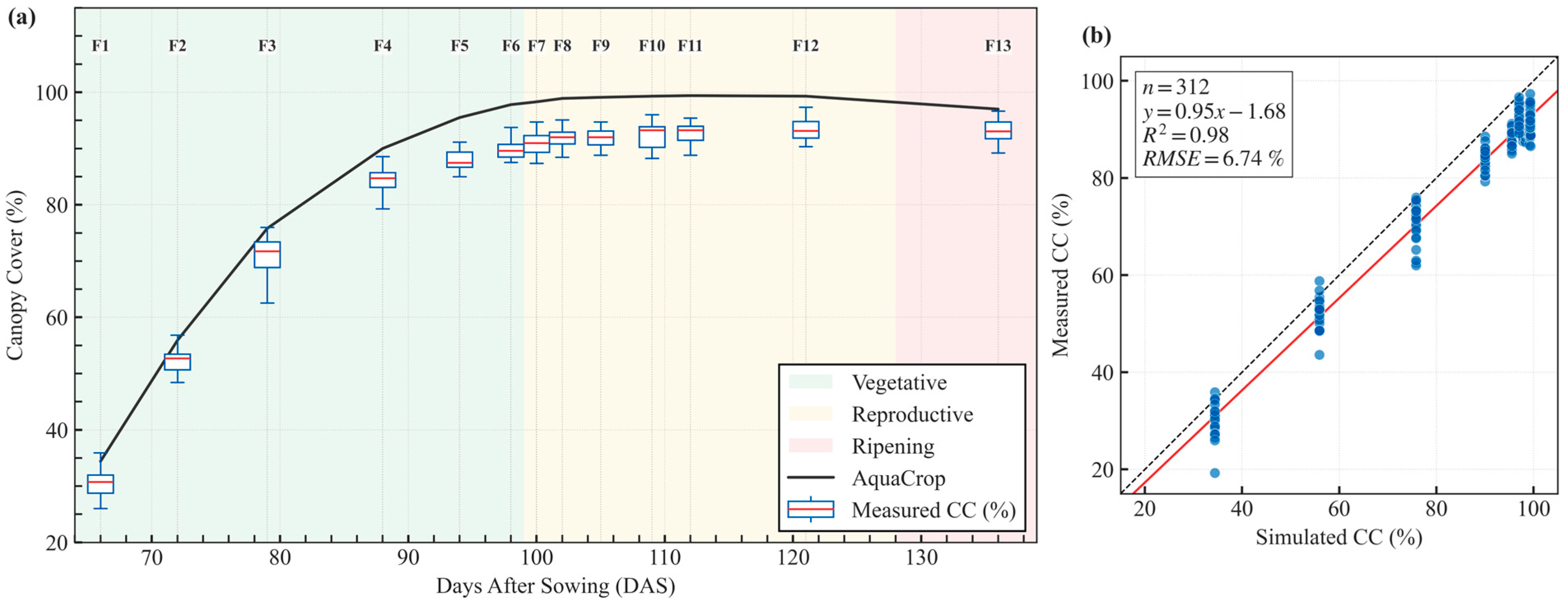
In parallel, the temporal evolution of Canopy Cover (CC) simulated by AquaCrop was rigorously validated against in situ observations to ensure the reliability of the transpiration component. As shown in Figure 8, the model successfully reproduced the rapid vegetative expansion; however, a systematic divergence was observed as the crop approached canopy closure.

Figure 8a illustrates that, while the simulated curve (solid line) closely tracks the observed growth trend during the early stages, it consistently overestimates the maximum canopy cover during the reproductive and ripening phases. The model simulates an idealized, uniform closure (~99%), whereas UAV observations reflect the natural heterogeneity of the field, where canopy cover saturates at slightly lower values (~90–95%).

This behavior is confirmed by the regression analysis in Figure 8b, where a clear clustering of data points below the 1:1 identity line is evident for CC values exceeding 80%. Despite this systematic bias towards overprediction at high cover levels, the statistical performance remains robust ($R^2$ = 0.98, RMSE = 6.74%). Crucially, this discrepancy has a negligible impact on daily transpiration estimates, as radiative interception and transpiration rates are effectively saturated at these high cover fractions (>90%), rendering the flux partitioning insensitive to minor variations in canopy closure.

3.3. Surface Energy Balance Partitioning

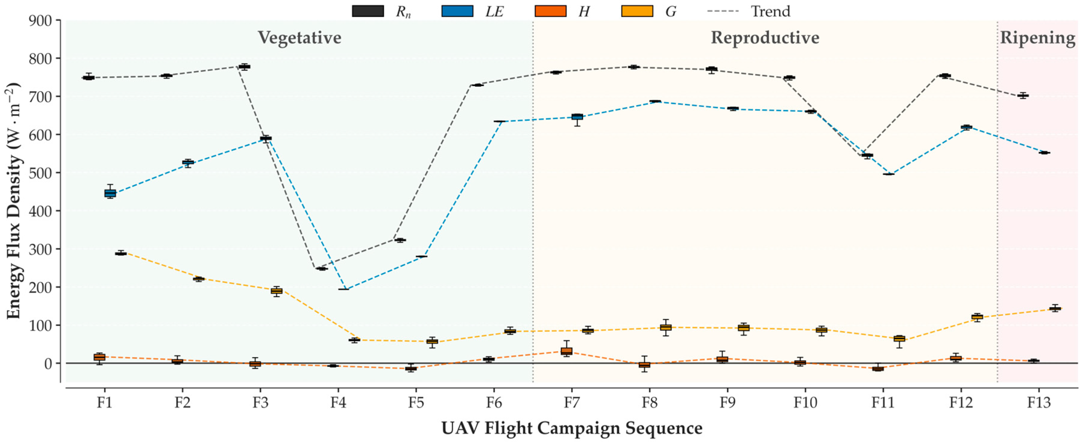
The temporal dynamics of instantaneous surface energy fluxes resolved by the TSEB model throughout the crop phenological cycle are presented in Figure 9.

The energy balance was consistently dominated by the latent heat flux (LE), which closely paralleled the trajectory of net radiation (Rn). During the reproductive stage (F7–F12), LE reached peak values ranging from 600 to 700 $\mathrm{W} {\mathrm{m}}^{-2}$, indicating that the majority of available energy was consumed by the vaporization process. This behavior is characteristic of rice agroecosystems under continuous flooding, where soil moisture is not a limiting factor for evapotranspiration. Conversely, the sensible heat flux (H) remained minimal (<100 $\mathrm{W} {\mathrm{m}}^{-2}$) throughout the season. Notably, H occasionally exhibited near-zero or negative values, suggesting the occurrence of local advection (oasis effect), a phenomenon typical in irrigated fields surrounded by arid environments. The soil heat flux (G) constituted a minor fraction of the total energy budget, progressively decreasing as canopy closure increased shading and attenuated the radiation reaching the soil surface.

3.4. Validation of Daily ET Against Drainage Lysimeters (ET_lys)

Daily evapotranspiration derived from the 24 drainage lysimeters (ET_lys) was used as the independent observational benchmark to evaluate both modeling approaches under the uniform continuous flooding (CF) treatment. To represent the treatment-level response and ensure scale consistency with the model outputs, lysimeter observations were aggregated as the mean across the 24 units for each day and for each UAV campaign. Direct model-to-lysimeter validation is presented in Figure 10, comparing ET_lys against (a) AquaCrop daily ET and (b) UAV–TSEB daily ET.

AquaCrop showed a near 1:1 agreement with ET_lys (Figure 10a), with strong explanatory power and minimal bias (R² = 0.85; RMSE = 0.26 mm d⁻¹; MBE = 0.01 mm d⁻¹), indicating that the calibrated canopy development and daily water-balance closure reproduced the lysimeter-mean behavior. UAV–TSEB captured the overall range and variability of ET_lys (Figure 10b) but exhibited greater dispersion and a systematic positive bias (R² = 0.66; RMSE = 0.81 mm d⁻¹; MBE = 1.01 mm d⁻¹), consistent with the instantaneous nature of thermal-based flux retrievals and subsequent temporal upscaling to daily ET. For completeness, the expanded comparison using the full paired dataset across lysimeters and dates is provided in the Supplementary Material (Figure S2), which further confirms the overall consistency of AquaCrop against ET_lys at larger sample size (R² = 0.87; RMSE = 0.26 mm d⁻¹; MBE = −0.02 mm d⁻¹).

3.5. Daily Evapotranspiration and E-T Partitioning: TSEB vs. AquaCrop

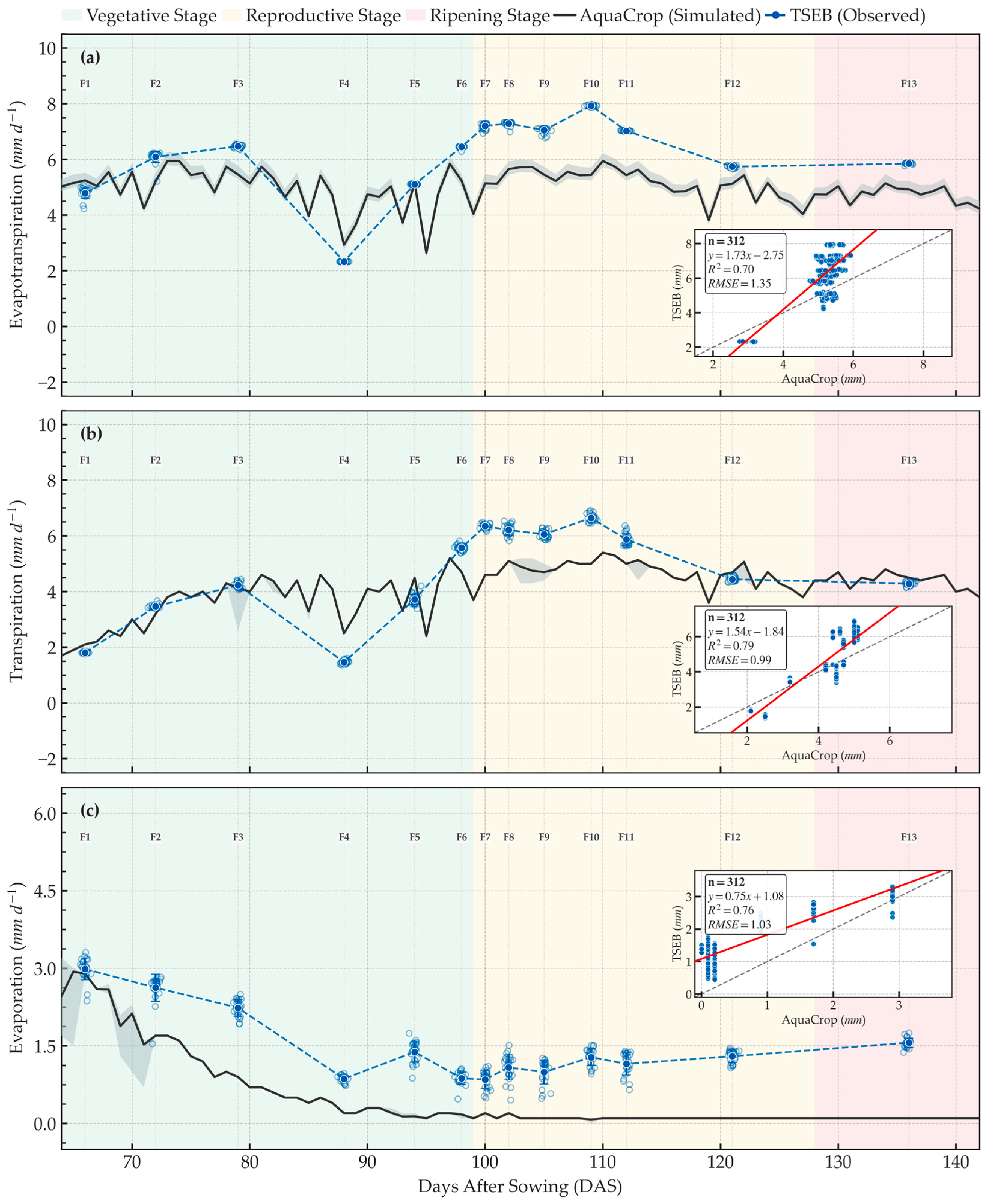
The comparative performance between the instantaneous remote sensing approach (TSEB) and the continuous water balance modeling (AquaCrop) for estimating daily evapotranspiration (${ET}_d$) and its partitioned components is systematically evaluated in Figure 11.

Regarding total evapotranspiration (Figure 11a), both models effectively captured the seasonal seasonality of crop water consumption, with rates fluctuating between 2.0 and 8.0 $\mathrm{m}\mathrm{m} {\mathrm{d}}^{-1}$. The TSEB model (blue markers) exhibited higher inter-daily variability, a behavior consistent with its sensitivity to instantaneous atmospheric forcing and surface skin temperature fluctuations at the time of flight. In contrast, AquaCrop (black solid line) generated a smoother temporal envelope, characteristic of models driven by daily climatic averages. Despite these conceptual differences in temporal resolution, the statistical correlation was satisfactory ($R^2$ = 0.70, RMSE = 1.35 $\mathrm{m}\mathrm{m} {\mathrm{d}}^{-1}$), confirming that the UAV-based energy balance successfully scaled to daily magnitudes.

The strength of the proposed integration becomes evident in the disaggregated flux analysis. For crop transpiration ($T_c$), illustrated in Figure 11b, a robust consistency was obtained ($R^2=0.79$, RMSE = 0.99 $\mathrm{m}\mathrm{m} {\mathrm{d}}^{-1}$), evidencing that both approaches correctly detected the surge in physiological activity and canopy conductance from the vegetative to the reproductive phase. Concurrently, soil evaporation (E) (Figure 11c) demonstrated a notable correlation ($R^2=0.76$), with both models accurately identifying the exponential decay in direct evaporation (<1.5 $\mathrm{m}\mathrm{m} {\mathrm{d}}^{-1}$) following canopy closure (approx. 80 DAS). These results validate the physical capability of the TSEB model to partition latent heat fluxes using solely radiometric temperature and structural vegetation indices without requiring local soil moisture sensors.

3.6. Spatiotemporal Distribution of Evapotranspiration

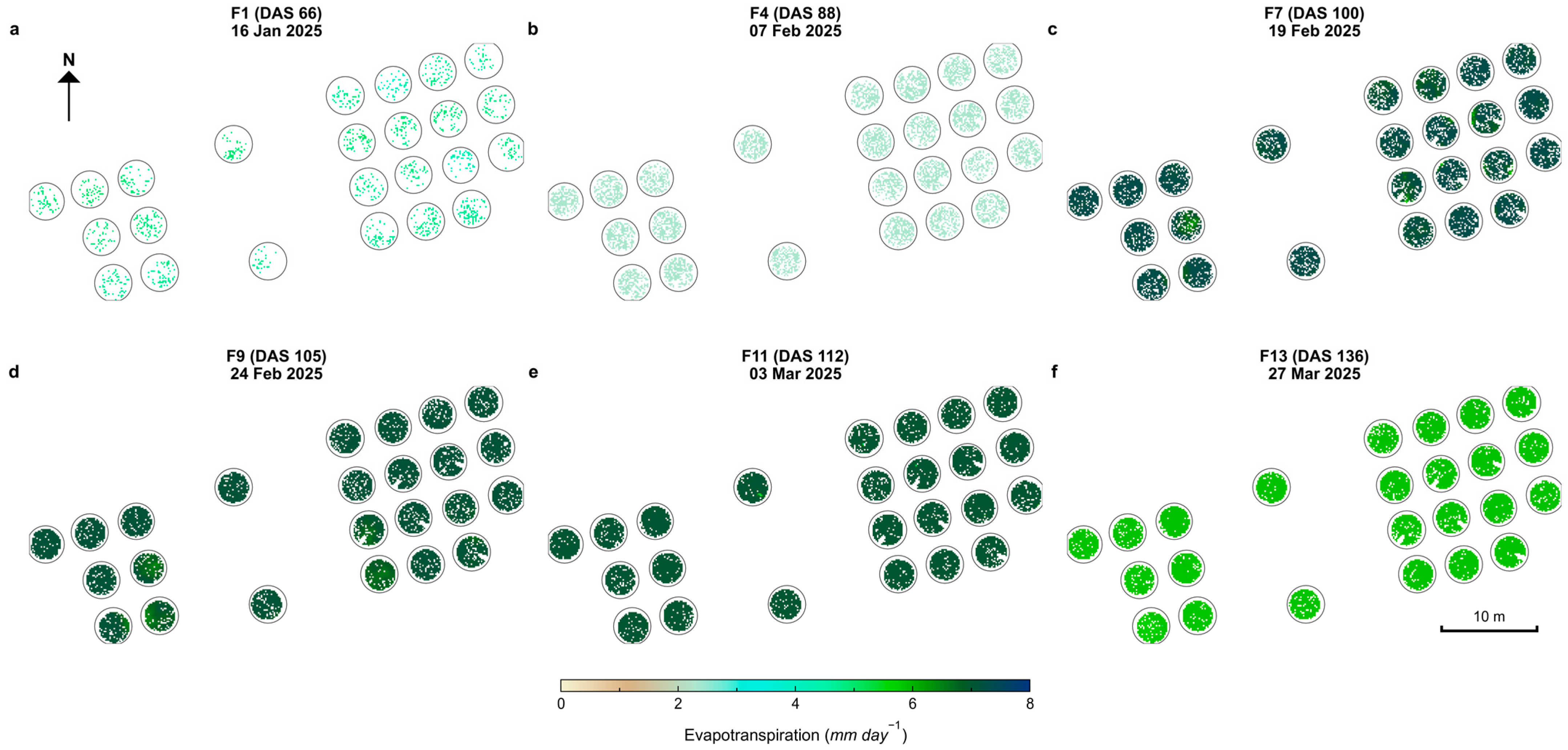
A definitive advantage of the UAV-TSEB framework over conventional point-based or 1D simulations (e.g., AquaCrop) is its capacity to resolve intra-plot spatial variability at the decimetric scale. The spatiotemporal evolution of daily evapotranspiration (${ET}_d$) across the lysimeter network is visualized in the high-resolution maps of Figure 11 (main phenological milestones) and Figure S3 (intermediate monitoring dates, available in Supplementary Material).

During the early vegetative stages (Figure 12, F1–F4; and Figure S3, F2–F5), the maps reveal a marked spatial heterogeneity in latent heat fluxes. In these initial phases (DAS 66–88), ${ET}_d$ rates remained moderate (<4.0 $\mathrm{m}\mathrm{m} {\mathrm{d}}^{-1}$, represented by light green tones), with significant intra-lysimeter variance. This “pixel-to-pixel” noise is attributable to the stochastic nature of crop establishment and the dominance of soil evaporation ($E$) in areas with incomplete canopy closure, where micro-variations in soil moisture and surface roughness exert a stronger influence on the radiometric temperature ($T_{rad}$) recorded by the thermal sensor.

As the crop progressed into the reproductive phase (Figure 12, F7–F11), a transition towards thermodynamic homogeneity was observed. Coinciding with canopy closure ($f_c\to 1.0$), the spatial distribution of ${ET}_d$ became highly uniform, reflecting the stabilization of the aerodynamic roughness length and the dominance of crop transpiration ($T$). During this peak demand period (DAS 100–112), evapotranspiration rates maximized, consistently exceeding 6.0 $\mathrm{m}\mathrm{m} {\mathrm{d}}^{-1}$ (dark green tones) across all experimental units. This spatial coalescence confirms that the TSEB model successfully captures the integration of the soil–plant–atmosphere continuum when the canopy is fully developed.

Finally, the onset of senescence during the ripening stage (Figure 12, F13; DAS 136) was detected spatially as a generalized reduction in flux density (shift to lighter green tones) and a re-emergence of spatial variability. This reduction corresponds to the physiological decline in stomatal conductance and the reduction in green leaf area. Crucially, this spatial characterization allows for the identification of sub-meter patterns—such as edge effects or localized water stress hotspots—that lumped-parameter models like AquaCrop inherently aggregate into a single scalar value, highlighting the potential of UAV thermography for precision irrigation auditing.

3.7. Yield Assessment and Water Productivity

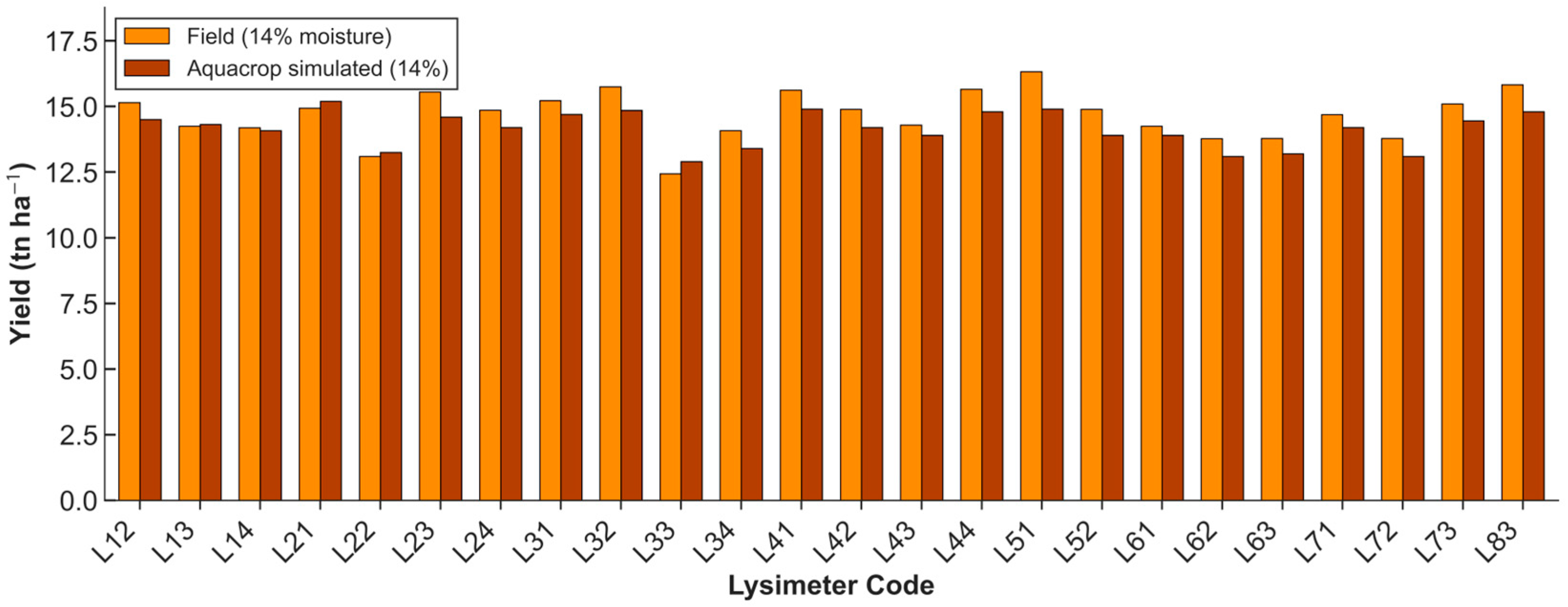
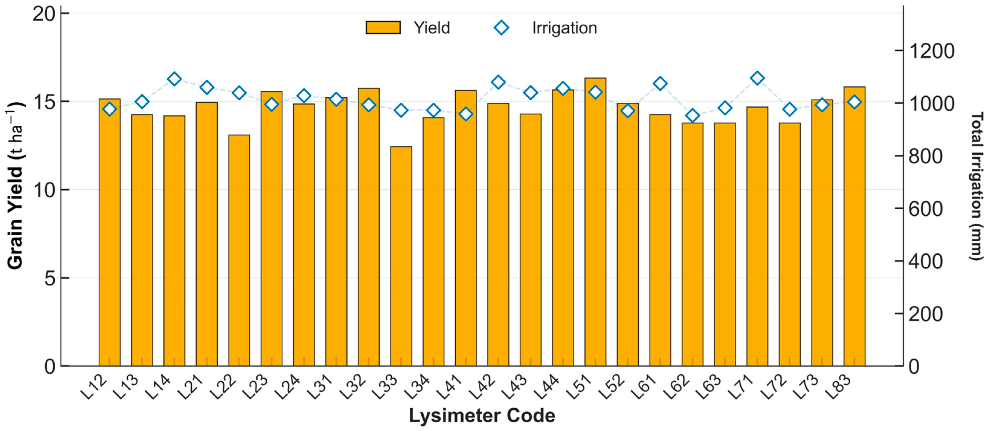
The ultimate validation of the proposed monitoring framework lies in its capacity to translate biophysical estimates into agronomic performance metrics. The assessment of grain yield and the subsequent analysis of Water Use Efficiency (WUE) are presented in Figure 13 and Figure 14.

As illustrated in Figure 13, the calibrated AquaCrop model demonstrated a robust predictive capability for grain yield across the lysimeter network under continuous flooding conditions. Simulated values (dark brown bars) closely approximated field observations (orange bars), with yields generally ranging between 12.5 and 16.0 $\mathrm{t} {\mathrm{h}\mathrm{a}}^{-1}$. The statistical agreement was high, with the model successfully capturing the high-yield potential of the study site (${Mean}_{obs}$ = 14.83 $\mathrm{t} {\mathrm{h}\mathrm{a}}^{-1}$ vs. ${Mean}_{sim}$ = 14.28 $\mathrm{t} {\mathrm{h}\mathrm{a}}^{-1}$). Minor discrepancies observed in specific units (e.g., L33, L34) may be attributed to local experimental variabilities—such as edge effects or micro-scale soil heterogeneities—that are not captured by the generalized conservative parameters of the model.

Complementing the yield analysis, Figure 14 integrates the production data with the total applied irrigation volume to assess the hydrological sustainability of the system. A remarkable consistency in productive response was observed, where high mean yields (>14 $\mathrm{t} {\mathrm{h}\mathrm{a}}^{-1}$) were sustained by irrigation depths varying narrowly between 900 and 1100 mm (blue diamonds). This relationship translates into an exceptionally high Water Use Efficiency (WUE), averaging 1.49 $\mathrm{k}\mathrm{g} {\mathrm{m}}^{-3}$. These values indicate that the continuous flooding management implemented, combined with the high radiation conditions of the Peruvian arid coast, maximized the conversion of water into biomass. The integration of these results confirms that the AquaCrop model, forced with local climatic data, not only correctly simulates physical water fluxes (ET) but also effectively translates crop water consumption into marketable biomass production.

4. Discussion

4.1. Divergence Between Instantaneous and Continuous Approaches

The complementary intercomparison between UAV–TSEB and the field-calibrated AquaCrop model showed satisfactory consistency for daily evapotranspiration (R² = 0.70; RMSE = 1.35 mm d⁻¹), comparable to deviations reported in studies integrating thermal remote sensing with crop or hydrological modeling in rice [3,8,43,44,45]. However, this agreement should be interpreted in the context of the validation hierarchy established in this study: ET derived from the 24 drainage lysimeters (ET_lys) constitutes the independent observational benchmark (Figure 10), whereas the UAV–TSEB vs. AquaCrop comparison (Figure 11) is used to interpret process consistency and model structural differences rather than to define “truth”.

The divergence observed between both approaches is physically expected. AquaCrop simulates ET from a daily soil–plant water balance constrained by internal state variables (canopy development, transpiration capacity, and stage-dependent soil evaporation), which yields a smooth temporal response reflecting the daily mean crop condition. In contrast, UAV–TSEB is an instantaneous energy-balance retrieval driven by radiometric surface temperature and contemporaneous atmospheric forcing near solar noon; therefore, it is more sensitive to short-lived micrometeorological variability during the acquisition window (e.g., wind fluctuations, transient cloud passages). This sensitivity is reflected in the higher inter-date variability of UAV–TSEB estimates around flight dates, while AquaCrop provides continuous daily stability.

A critical methodological refinement introduced in the revised manuscript is the temporal upscaling strategy. Daily ET from UAV–TSEB was not obtained using a constant evaporative fraction assumption, which is known to be sensitive under advective conditions, but rather using incoming solar radiation scaling (R_s), following the one-time-of-day integration concept proposed by [35] and further evaluated for agricultural applications [33,46]. Radiation-based scaling is operationally robust because it leverages the dominant radiative control around solar noon, and it has been validated in sUAS energy-balance contexts [47]. Nonetheless, any single-overpass approach remains potentially sensitive to afternoon departures driven by wind and vapor pressure deficit (VPD), which is particularly relevant in arid coastal environments.

Consistent with these expectations, both approaches captured energy-limited conditions during the F4 campaign, when a marked reduction in incoming solar radiation occurred due to transient cloud cover during the flight window (Figure 9; Table S2). The concurrent reduction in ET indicates that the coupled monitoring framework responds appropriately to short-term atmospheric forcing. Similarly, lower early-season fluxes were associated with sparse canopy cover (low $f_c$) when evaporation dominates the surface energy balance, consistent with phenological dynamics in rice.

4.2. Flux Partitioning in Flooded Rice: Agreement and Systematic Divergence

A key strength of the two-source formulation is its ability to partition radiometric temperature into soil and canopy components, enabling separate estimation of soil evaporation (E_s) and canopy transpiration (T_c) [17,18]. The UAV–TSEB vs. AquaCrop intercomparison shows robust consistency in seasonal partitioning dynamics (T_c: R² = 0.79; RMSE = 0.99 mm d⁻¹; E_s: R² = 0.76; RMSE = 1.03 mm d⁻¹; Figure 10), and both approaches identified the transition near canopy closure (~80 DAS) when transpiration becomes dominant and direct evaporation decreases due to shading.

Importantly, the study reveals a systematic divergence under near-complete canopy cover in flooded conditions: AquaCrop tends to suppress E_s to negligible levels, whereas UAV–TSEB detects residual evaporation from the flooded surface. This behavior is consistent with structural differences between a physically explicit energy-balance residual (UAV–TSEB) and a conceptual evaporation scheme constrained by canopy cover (AquaCrop) [48]. Under flooded rice, evaporation can persist even at high $f_c$ due to free-water surfaces, micro-openings, and advective enhancement; such contributions can be captured by an energy-balance residual but may be minimized in a canopy-dominated water-balance model.

At the same time, when $f_c\to 1$, thermal disaggregation becomes increasingly sensitive because the soil contribution to the radiometric signal is attenuated. Small uncertainties in $f_c$, LAI, canopy architecture, or view geometry can propagate into the soil/canopy temperature split and the resulting E–T partition [19,30,33,49]. This sensitivity likely contributes to the positive bias observed in UAV–TSEB against ET_lys (Figure 10b), particularly during dense canopy stages when the radiometric separation is least constrained.

4.3. Implications of Sub-Metric Resolution and Spatial Analysis

Although TSEB was originally developed under micrometeorological assumptions typically applied at coarser spatial scales, recent UAV and sharpened-TIR applications show that sub-metric to metric resolutions (≈0.06–1 m) provide an effective trade-off: they reduce thermal noise while preserving spatially meaningful gradients in LST and ET relevant for irrigation management [20,50,51,52]. Consistent with this evidence, implementing UAV–TSEB at 0.15 m in this study yielded hundreds of thermal pixels per lysimeter unit, and aggregating model outputs to the lysimeter footprint attenuated pixel-level variability while maintaining within-treatment contrasts. This aggregation strategy aligns with common UAV-to-field and UAV-to-flux-footprint validation practices and enables a coherent comparison at the hydrologically relevant management unit [3,20,49].

The resulting ET maps highlight the operational value of UAV–TSEB as a spatial diagnostic tool. Early in the season, incomplete canopy cover produced marked spatial heterogeneity driven by micro-variations in surface conditions and vegetation establishment, whereas canopy closure led to a more homogeneous, transpiration-dominated ET field. The re-emergence of spatial variability during senescence further underscores the ability of thermal observations to detect localized deviations that may remain hidden to lumped daily simulations, supporting precision irrigation auditing and targeted management interventions [20,53,54].

4.4. Synergies for Precision Irrigation Management

The findings indicate that UAV–TSEB and AquaCrop should be viewed as complementary components of a unified precision irrigation monitoring framework rather than competing alternatives. Under continuous flooding, AquaCrop provides a robust temporal backbone by delivering continuous daily estimates for seasonal planning, irrigation accounting, and yield forecasting; its near-unbiased agreement with the lysimeter benchmark (ET_lys; Figure 10a) supports its operational reliability at the treatment scale. In contrast, UAV–TSEB functions as a high-fidelity spatial diagnostic layer, generating radiometrically driven snapshots that resolve intra-field variability in ET and support the interpretation of productive transpiration ($T_c$) versus non-productive evaporation ($E_s$) losses (Figure 11), which are difficult to infer from lumped daily simulations alone [47,55].

This hybrid strategy bridges two key limitations: the lack of sub-field spatial detail in crop models and the temporal discontinuity inherent to UAV campaigns. Practically, UAV–TSEB maps can be used to identify spatial anomalies (e.g., localized heterogeneity in canopy development or surface conditions) and to update canopy-related parameters (e.g., CC/$f_c$) that control transpiration dynamics in AquaCrop, consistent with recent assimilation efforts where remote-sensing-derived canopy metrics improved crop-model performance [56,57,58]. Our results therefore support recent spatiotemporal ET monitoring frameworks that combine physically based energy-balance retrievals with crop modeling to strengthen irrigation diagnostics and water-use efficiency assessments in arid agroecosystems [3,5,59,60].

4.5. Limitations and Future Perspectives

Although the coupled UAV–TSEB and AquaCrop framework proved robust for daily ET estimation and flux partitioning, several limitations should be acknowledged to contextualize the results and guide future work.

Temporal upscaling. Daily ET from UAV–TSEB requires converting an instantaneous, near-solar-noon retrieval into a 24 h total. In this study, we used incoming solar radiation scaling ($R_s$), which avoids relying on a constant evaporative fraction (EF) and is operationally stable under radiatively dominated conditions. Nevertheless, single-overpass upscaling remains a key source of uncertainty when afternoon advection intensifies or surface–atmosphere coupling changes rapidly. Future work should evaluate advanced diurnal integration approaches that explicitly incorporate atmospheric coupling and meteorological dynamics (e.g., constant decoupling factor formulations) and/or exploit multiple observations per day through multi-platform fusion [46,61]. In addition, commonly used diurnal EF-based approaches driven by hourly meteorological forcing (radiation, VPD, wind), including formulations that account for surface–atmosphere coupling [62], should be evaluated as alternatives to single-overpass upscaling [62]. Where feasible, continuous flux measurements (e.g., eddy covariance) would provide an independent constraint to quantify and correct diurnal scaling biases under advective coastal conditions [48].

Dense-canopy partitioning under flooding. When fractional cover approaches unity ($f_c\to 1$) in flooded rice, radiometric disaggregation becomes increasingly sensitive because the soil/water contribution to $T_{\mathrm{r}\mathrm{a}\mathrm{d}}$ is attenuated. Consequently, uncertainties in canopy structure (LAI, $f_c$, architecture) and view geometry can propagate into the soil–canopy temperature split and affect the residual evaporation component. Incorporating additional constraints on canopy structure (improved LAI/$f_c$ retrievals, shadow-aware thermal preprocessing, or multi-angle information) could reduce partitioning uncertainty, particularly during reproductive stages.

Operational scalability. While this study provides rigorous plot-scale validation using a lysimeter network, scaling the framework to operational decision support remains a priority. Two directions are especially promising: (i) automated assimilation pipelines to update AquaCrop states (e.g., canopy development and ET constraints) with UAV-derived products, reducing the need for manual recalibration; and (ii) multi-scale integration in which UAV-calibrated parameters and bias information inform satellite-based ET products (e.g., Sentinel-2/3 and Landsat) for irrigation-district applications [49,59,61,62].

5. Conclusions

This study integrated UAV-based thermal–multispectral observations with a two-source energy balance model (UAV–TSEB) and a field-calibrated AquaCrop simulation to estimate daily evapotranspiration and its components in flooded rice during the 2024–2025 season on the arid Peruvian coast. A network of 24 drainage lysimeters provided an independent observational benchmark (ET_lys) and enabled a clear validation hierarchy: both AquaCrop and UAV–TSEB were directly evaluated against lysimeter-derived ET (Figure 10), while the UAV–TSEB vs. AquaCrop analysis was used as a complementary intercomparison for interpreting flux partitioning (Figure 11).

Direct lysimeter validation indicated high accuracy and negligible bias for AquaCrop (R² = 0.85; RMSE = 0.26 mm d⁻¹; MBE = 0.01 mm d⁻¹), supporting its role as a reliable daily simulator under continuous flooding. UAV–TSEB captured the overall magnitude and variability of ET_lys but showed larger dispersion and a positive bias (R² = 0.66; RMSE = 0.81 mm d⁻¹; MBE = 1.01 mm d⁻¹), consistent with the sensitivity of instantaneous thermal-based retrievals and subsequent temporal upscaling. The intercomparison between both approaches showed coherent seasonal dynamics in total ET and robust behavior in E–T partitioning while revealing a systematic divergence under near-complete canopy cover: AquaCrop tends to suppress evaporation, whereas UAV–TSEB detects residual evaporation from the flooded surface.

Overall, the findings highlight a practical complementarity: AquaCrop provides daily continuity for planning and scenario analysis, while UAV–TSEB provides spatial diagnostics and physically based partitioning of evapotranspiration components. Future research should focus on refining daily upscaling under advective conditions, reducing dense-canopy partitioning uncertainty in flooded systems, and developing automated assimilation and multi-scale integration pathways to extend UAV-calibrated insights to satellite-based operational monitoring.

References

1. Quispe-Tito, D.J.; Ramos-Fernández, L.; Pino-Vargas, E.; Quille-Mamani, J.; Torres-Rua, A. Use of RPAS for Precision Evapotranspiration in Rice Fields and Water Consumption Reduction. Agron. Mesoam. 2024, 35. [Google Scholar] [CrossRef] [Scilit]
2. Sara, O.; Bouchra, A.; Abdelhakim, A.; Salah, E.R.A.K.I.; Lhoussaine, B.; Frederic, J.; Abdelghani, C. Assessment of the Modified Two-Source Energy Balance (TSEB) Model for Estimating Evapotranspiration and Its Components over an Irrigated Olive Orchard in Morocco. Agric. Water Manag. 2024, 298, 108861. [Google Scholar] [CrossRef] [Scilit]
3. Tao, S.; Song, L.; Zhao, G.; Zhao, L. Simulation and Assessment of Daily Evapotranspiration in the Heihe River Basin over a Long Time Series Based on TSEB-SM. Remote Sens. 2024, 16, 462. [Google Scholar] [CrossRef] [Scilit]
4. Unnisa, Z.; Govind, A.; Prikaziuk, E.; Van der Tol, C.; Lasserre, B.; Burchard-Levine, V.; Marchetti, M. Assessing Evapotranspiration Models for Regional Implementation in the Mediterranean: A Comparative Analysis of STEPS, TSEB, and SCOPE with Global Datasets. Appl. Sci. 2024, 14, 7685. [Google Scholar] [CrossRef] [Scilit]
5. Ramos-Fernández, L.; Peña-Amaro, R.; Huanuqueño-Murillo, J.; Quispe-Tito, D.; Maldonado-Huarhuachi, M.; Heros-Aguilar, E.; Flores del Pino, L.; Pino-Vargas, E.; Quille-Mamani, J.; Torres-Rua, A. Water Use Efficiency in Rice Under Alternative Wetting and Drying Technique Using Energy Balance Model with UAV Information and AquaCrop in Lambayeque, Peru. Remote Sens. 2024, 16, 3882. [Google Scholar] [CrossRef] [Scilit]
6. Ramos-Fernández, L.; Quispe-Tito, D.; Altamirano-Gutiérrez, L.; Cruz-Grimaldo, C.; Quille-Mamani, J.A.; Carbonell-Rivera, J.P.; Torralba, J.; Ruiz, L.Á. Estimation of Evapotranspiration from High-Resolution UAV Images for Irrigation Systems in Rice Fields on the Northern Coast of Peru. Sci. Agropecu. 2024, 15, 7–21. [Google Scholar] [CrossRef] [Scilit]
7. Ramos-Fernández, L.; Gonzales-Quiquia, M.; Huanuqueño-Murillo, J.; Tito-Quispe, D.; Heros-Aguilar, E.; Flores del Pino, L.; Torres-Rua, A. Water Stress Index and Stomatal Conductance under Different Irrigation Regimes with Thermal Sensors in Rice Fields on the Northern Coast of Peru. Remote Sens. 2024, 16, 796. [Google Scholar] [CrossRef] [Scilit]
8. Quille-Mamani, J.A.; Ramos-Fernández, L.; Ontiveros-Capurata, R.E. Estimation of Rice Crop Evapotranspiration in Perú Based on the Metric Algorithm and UAV Images. Rev. Teledetec. 2021, 2021, 23–38. [Google Scholar] [CrossRef] [Scilit]
9. Quintanilla-Albornoz, M.; Miarnau, X.; Pelechá, A.; Casadesús, J.; García-Tejera, O.; Bellvert, J. Evaluation of Transpiration in Different Almond Production Systems with Two-Source Energy Balance Models from UAV Thermal and Multispectral Imagery. Irrig. Sci. 2023, 43, 29–49. [Google Scholar] [CrossRef] [Scilit]
10. Tunca, E. Evaluating the Performance of the TSEB Model for Sorghum Evapotranspiration Estimation Using Time Series UAV Imagery. Irrig. Sci. 2023, 42, 977–994. [Google Scholar] [CrossRef] [Scilit]
11. Jofre-Cekalovic, C.; Nieto, H.; Girona, J.; Pamies-Sans, M.; Bellvert, J. Accounting for Almond Crop Water Use under Different Irrigation Regimes with a Two-Source Energy Balance Model and Copernicus-Based Inputs. Remote Sens. 2022, 14, 2106. [Google Scholar] [CrossRef] [Scilit]
12. Tang, R.; Li, Z.L.; Tang, B. An Application of the Ts–VI Triangle Method with Enhanced Edges Determination for Evapotranspiration Estimation from MODIS Data in Arid and Semi-Arid Regions: Implementation and Validation. Remote Sens. Environ. 2010, 114, 540–551. [Google Scholar] [CrossRef] [Scilit]
13. Peng, Z.; Tang, R.; Jiang, Y.; Liu, M.; Li, Z.L. Global Estimates of 500 m Daily Aerodynamic Roughness Length from MODIS Data. ISPRS J. Photogramm. Remote Sens. 2022, 183, 336–351. [Google Scholar] [CrossRef] [Scilit]
14. Tang, R.; Li, Z.L.; Liu, M.; Jiang, Y.; Peng, Z. A Moisture-Based Triangle Approach for Estimating Surface Evaporative Fraction with Time-Series of Remotely Sensed Data. Remote Sens. Environ. 2022, 280, 113212. [Google Scholar] [CrossRef] [Scilit]
15. Bastiaanssen, W.G.M.; Menenti, M.; Feddes, R.A.; Holtslag, A.A.M. A Remote Sensing Surface Energy Balance Algorithm for Land (SEBAL). 1. Formulation. J. Hydrol. 1998, 212–213, 198–212. [Google Scholar] [CrossRef] [Scilit]
16. Allen, R.G.; Tasumi, M.; Trezza, R. Satellite-Based Energy Balance for Mapping Evapotranspiration with Internalized Calibration (METRIC)—Model. J. Irrig. Drain. Eng. 2007, 133, 380–394. [Google Scholar] [CrossRef] [Scilit]
17. Norman, J.M.; Kustas, W.P.; Humes, K.S. Source Approach for Estimating Soil and Vegetation Energy Fluxes in Observations of Directional Radiometric Surface Temperature. Agric. For. Meteorol. 1995, 77, 263–293. [Google Scholar] [CrossRef] [Scilit]
18. Kustas, W.P.; Norman, J.M. Evaluation of Soil and Vegetation Heat Flux Predictions Using a Simple Two-Source Model with Radiometric Temperatures for Partial Canopy Cover. Agric. For. Meteorol. 1999, 94, 13–29. [Google Scholar] [CrossRef] [Scilit]
19. Anderson, M.C.; Kustas, W.P.; Norman, J.M.; Diak, G.T.; Hain, C.R.; Gao, F.; Yang, Y.; Knipper, K.R.; Xue, J.; Yang, Y.; et al. A Brief History of the Thermal IR-Based Two-Source Energy Balance (TSEB) Model—Diagnosing Evapotranspiration from Plant to Global Scales. Agric. For. Meteorol. 2024, 350, 109951. [Google Scholar] [CrossRef] [Scilit]
20. Peng, J.; Nieto, H.; Neumann Andersen, M.; Kørup, K.; Larsen, R.; Morel, J.; Parsons, D.; Zhou, Z.; Manevski, K. Accurate Estimates of Land Surface Energy Fluxes and Irrigation Requirements from UAV-Based Thermal and Multispectral Sensors. ISPRS J. Photogramm. Remote Sens. 2023, 198, 238–254. [Google Scholar] [CrossRef] [Scilit]
21. Jaafar, H.H.; Sujud, L.H. High Resolution Evapotranspiration from UAV Multispectral Thermal Imagery: Validation and Comparison with EC, Landsat, and Fused S2-MODIS HSEB ET. Int. J. Appl. Earth Obs. Geoinf. 2025, 136, 104359. [Google Scholar] [CrossRef] [Scilit]
22. Nieto, H.; Kustas, W.P.; Torres-Rúa, A.; Alfieri, J.G.; Gao, F.; Anderson, M.C.; White, W.A.; Song, L.; Alsina, M.D.; Prueger, J.H.; et al. Evaluation of TSEB Turbulent Fluxes Using Different Methods for the Retrieval of Soil and Canopy Component Temperatures from UAV Thermal and Multispectral Imagery. Irrig. Sci. 2018, 37, 389–406. [Google Scholar] [CrossRef] [Scilit] [PubMed]
23. Porras-Jorge, R.; Ramos-Fernández, L.; Ojeda-Bustamante, W.; Ontiveros-Capurata, R.E. Performance Assessment of the AquaCrop Model to Estimate Rice Yields under Alternate Wetting and Drying Irrigation in the Coast of Peru. Sci. Agropecu. 2020, 11, 309–321. [Google Scholar] [CrossRef] [Scilit]
24. Heros, E.; Gómez, L.; Sosa, G. Use of Selection Indices in the Identification of Drought Tolerant Rice (Oryza sativa L.) Genotypes. Agric. Prod. Sustain. Dev. 2014, 2, 11–31. [Google Scholar] [CrossRef] [Scilit]
25. Machaca-Pillaca, R.; Pino-Vargas, E.; Ramos-Fernández, L.; Quille-Mamani, J.; Torres-Rua, A.; Machaca-Pillaca, R.; Pino-Vargas, E.; Ramos-Fernández, L.; Quille-Mamani, J.; Torres-Rua, A. Estimation of Evapotranspiration for Irrigation Purposes in Real Time of an Olive Grove from Drone Images in Arid Arcas, Case of La Yarada, Tacna, Peru. Idesia 2022, 40, 55–65. [Google Scholar] [CrossRef] [Scilit]
26. Kustas, W.P.; Norman, J.M. Use of Remote Sensing for Evapotranspiration Monitoring over Land Surfaces. Hydrol. Sci. J. 1996, 41, 495–516. [Google Scholar] [CrossRef] [Scilit]
27. Priestley, C.H.B.; Taylor, R.J. On the Assessment of Surface Heat Flux and Evaporation Using Large-Scale Parameters. Mon. Weather Rev. 1972, 100, 81–92. [Google Scholar] [CrossRef] [Scilit]
28. Choi, M.; Kustas, W.P.; Anderson, M.C.; Allen, R.G.; Li, F.; Kjaersgaard, J.H. An Intercomparison of Three Remote Sensing-Based Surface Energy Balance Algorithms over a Corn and Soybean Production Region (Iowa, U.S.) during SMACEX. Agric. For. Meteorol. 2009, 149, 2082–2097. [Google Scholar] [CrossRef] [Scilit]
29. French, A.N.; Hunsaker, D.J.; Thorp, K.R. Remote Sensing of Evapotranspiration over Cotton Using the TSEB and METRIC Energy Balance Models. Remote Sens. Environ. 2015, 158, 281–294. [Google Scholar] [CrossRef] [Scilit]
30. Colaizzi, P.D.; Kustas, W.P.; Anderson, M.C.; Agam, N.; Tolk, J.A.; Evett, S.R.; Howell, T.A.; Gowda, P.H.; O’Shaughnessy, S.A. Two-Source Energy Balance Model Estimates of Evapotranspiration Using Component and Composite Surface Temperatures. Adv. Water Resour. 2012, 50, 134–151. [Google Scholar] [CrossRef] [Scilit]
31. Song, L.; Liu, S.; Kustas, W.P.; Zhou, J.; Xu, Z.; Xia, T.; Li, M. Application of Remote Sensing-Based Two-Source Energy Balance Model for Mapping Field Surface Fluxes with Composite and Component Surface Temperatures. Agric. For. Meteorol. 2016, 230–231, 8–19. [Google Scholar] [CrossRef] [Scilit]
32. Xia, T.; Kustas, W.P.; Anderson, M.C.; Alfieri, J.G.; Gao, F.; McKee, L.; Prueger, J.H.; Geli, H.M.E.; Neale, C.M.U.; Sanchez, L.; et al. Mapping Evapotranspiration with High-Resolution Aircraft Imagery over Vineyards Using One-and Two-Source Modeling Schemes. Hydrol. Earth Syst. Sci. 2016, 20, 1523–1545. [Google Scholar] [CrossRef] [Scilit]
33. Colaizzi, P.D.; Evett, S.R.; Howell, T.A.; Li, F.; Kustas, W.P.; Anderson, M.C. Radiation Model for Row Crops: I. Geometric View Factors and Parameter Optimization. Agron. J. 2012, 104, 225–240. [Google Scholar] [CrossRef] [Scilit]
34. Timmermans, W.J.; Kustas, W.P.; Anderson, M.C.; French, A.N. An Intercomparison of the Surface Energy Balance Algorithm for Land (SEBAL) and the Two-Source Energy Balance (TSEB) Modeling Schemes. Remote Sens. Environ. 2007, 108, 369–384. [Google Scholar] [CrossRef] [Scilit]
35. Jackson, R.D.; Hatfield, J.L.; Reginato, R.J.; Idso, S.B.; Pinter, P.J. Estimation of Daily Evapotranspiration from One Time-of-Day Measurements. Dev. Agric. Manag. For. Ecol. 1983, 12, 351–362. [Google Scholar] [CrossRef] [Scilit]
36. Guzinski, R.; Nieto, H.; Jensen, R.; Mendiguren, G. Remotely Sensed Land-Surface Energy Fluxes at Sub-Field Scale in Heterogeneous Agricultural Landscape and Coniferous Plantation. Biogeosciences 2014, 11, 5021–5046. [Google Scholar] [CrossRef] [Scilit]
37. Elsadek, E.; Zhang, K.; Mousa, A.; Ezaz, G.T.; Tola, T.L.; Shaghaleh, H.; Hamad, A.A.A.; Alhaj Hamoud, Y. Study on the In-Field Water Balance of Direct-Seeded Rice with Various Irrigation Regimes under Arid Climatic Conditions in Egypt Using the AquaCrop Model. Agronomy 2023, 13, 609. [Google Scholar] [CrossRef] [Scilit]
38. Zhang, J.; Ding, Y.; Zhu, L.; Wan, Y.; Chai, M.; Ding, P. Estimating and Forecasting Daily Reference Crop Evapotranspiration in China with Temperature-Driven Deep Learning Models. Agric. Water Manag. 2025, 307, 109268. [Google Scholar] [CrossRef] [Scilit]
39. Moratiel, R.; Bravo, R.; Saa, A.; Tarquis, A.M.; Almorox, J. Estimation of Evapotranspiration by the Food and Agricultural Organization of the United Nations (FAO) Penman-Monteith Temperature (PMT) and Hargreaves-Samani (HS) Models under Temporal and Spatial Criteria—A Case Study in Duero Basin (Spain). Nat. Hazards Earth Syst. Sci. 2020, 20, 859–875. [Google Scholar] [CrossRef] [Scilit]
40. Wang, Y.; Ma, R.; Vereecken, H. A Generalized Framework to Describe Unimodal and Bimodal Soil Hydraulic Properties Over Full Water Saturation Range. Water Resour. Res. 2025, 61, e2024WR038450. [Google Scholar] [CrossRef] [Scilit]
41. Maniruzzaman, M.; Talukder, M.S.U.; Khan, M.H.; Biswas, J.C.; Nemes, A. Validation of the AquaCrop Model for Irrigated Rice Production under Varied Water Regimes in Bangladesh. Agric. Water Manag. 2015, 159, 331–340. [Google Scholar] [CrossRef] [Scilit]
42. Schmidt, M.; Lipson, H. Distilling Free-Form Natural Laws from Experimental Data. Science 2009, 324, 81–85. [Google Scholar] [CrossRef] [Scilit] [PubMed]
43. Bozorgi, M.; Cristóbal, J.; Pàmies-Sans, M. Evaluating the Two-Source Energy Balance Model Using MODIS Data for Estimating Evapotranspiration Time Series on a Regional Scale. Remote Sens. 2024, 16, 4587. [Google Scholar] [CrossRef] [Scilit]
44. Chen, D.; Zhuang, Q.; Zhang, W.; Zhu, L. Estimation of Landsat-like Daily Evapotranspiration for Crop Water Consumption Monitoring Using TSEB Model and Data Fusion. PLoS ONE 2022, 17, e0267811. [Google Scholar] [CrossRef] [Scilit]
45. Wei, G.; Cao, J.; Xie, H.; Xie, H.; Yang, Y.; Wu, C.; Cui, Y.; Luo, Y. Spatial-Temporal Variation in Paddy Evapotranspiration in Subtropical Climate Regions Based on the SEBAL Model: A Case Study of the Ganfu Plain Irrigation System, Southern China. Remote Sens. 2022, 14, 1201. [Google Scholar] [CrossRef] [Scilit]
46. Nassar, A.; Torres-rua, A.; Kustas, W.; Alfieri, J.; Hipps, L.; Prueger, J.; Nieto, H.; Alsina, M.M.; White, W.; McKee, L.; et al. Assessing Daily Evapotranspiration Methodologies from One-Time-of-Day SUAS and EC Information in the GRAPEX Project. Remote Sens. 2021, 13, 2887. [Google Scholar] [CrossRef] [Scilit]
47. Meza, K.; Torres-Rua, A.F.; Hipps, L.; Kustas, W.P.; Gao, R.; Christiansen, L.; Kopp, K.; Nieto, H.; Burchard-Levine, V.; Martín, M.P.; et al. Spatial Estimation of Actual Evapotranspiration over Irrigated Turfgrass Using SUAS Thermal and Multispectral Imagery and TSEB Model. Irrig. Sci. 2023, 43, 5–28. [Google Scholar] [CrossRef] [Scilit]
48. Vanuytrecht, E.; Raes, D.; Steduto, P.; Hsiao, T.C.; Fereres, E.; Heng, L.K.; Garcia Vila, M.; Mejias Moreno, P. AquaCrop: FAO’s Crop Water Productivity and Yield Response Model. Environ. Model. Softw. 2014, 62, 351–360. [Google Scholar] [CrossRef] [Scilit]
49. Guzinski, R.; Nieto, H.; Sandholt, I.; Karamitilios, G. Modelling High-Resolution Actual Evapotranspiration through Sentinel-2 and Sentinel-3 Data Fusion. Remote Sens. 2020, 12, 1433. [Google Scholar] [CrossRef] [Scilit]
50. Kustas, W.P.; Nieto, H.; Garcia-Tejera, O.; Bambach, N.; McElrone, A.J.; Gao, F.; Alfieri, J.G.; Hipps, L.E.; Prueger, J.H.; Torres-Rua, A.; et al. Impact of Advection on Two-Source Energy Balance (TSEB) Canopy Transpiration Parameterization for Vineyards in the California Central Valley. Irrig. Sci. 2022, 40, 575–591. [Google Scholar] [CrossRef] [Scilit]
51. Simpson, J.E.; Holman, F.; Nieto, H.; Voelksch, I.; Mauder, M.; Klatt, J.; Fiener, P.; Kaplan, J.O. High Spatial and Temporal Resolution Energy Flux Mapping of Different Land Covers Using an Off-the-Shelf Unmanned Aerial System. Remote Sens. 2021, 13, 1286. [Google Scholar] [CrossRef] [Scilit]
52. Kustas, W.P.; Alfieri, J.G.; Nieto, H.; Wilson, T.G.; Gao, F.; Anderson, M.C. Utility of the Two-Source Energy Balance (TSEB) Model in Vine and Interrow Flux Partitioning over the Growing Season. Irrig. Sci. 2018, 37, 375–388. [Google Scholar] [CrossRef] [Scilit]
53. Bellvert, J.; Jofre-Ĉekalović, C.; Pelechá, A.; Mata, M.; Nieto, H. Feasibility of Using the Two-Source Energy Balance Model (TSEB) with Sentinel-2 and Sentinel-3 Images to Analyze the Spatio-Temporal Variability of Vine Water Status in a Vineyard. Remote Sens. 2020, 12, 2299. [Google Scholar] [CrossRef] [Scilit]
54. Gao, R.; Torres-Rua, A.F.; Nieto, H.; Zahn, E.; Hipps, L.; Kustas, W.P.; Alsina, M.M.; Bambach, N.; Castro, S.J.; Prueger, J.H.; et al. ET Partitioning Assessment Using the TSEB Model and SUAS Information across California Central Valley Vineyards. Remote Sens. 2023, 15, 756. [Google Scholar] [CrossRef] [Scilit]
55. Niu, H.; Chen, Y.Q. Towards Tree-Level Evapotranspiration Estimation with Small UAVs in Precision Agriculture; Springer Nature: Berlin/Heidelberg, Germany, 2022; pp. 1–156. [Google Scholar] [CrossRef] [Scilit]
56. Jin, X.; Li, Z.; Feng, H.; Ren, Z.; Li, S. Estimation of Maize Yield by Assimilating Biomass and Canopy Cover Derived from Hyperspectral Data into the AquaCrop Model. Agric. Water Manag. 2020, 227, 105846. [Google Scholar] [CrossRef] [Scilit]
57. Li, W.; Li, M.; Awais, M.; Ji, L.; Li, H.; Song, R.; Cheema, M.J.M.; Agarwal, R. Research on Assimilation of Unmanned Aerial Vehicle Remote Sensing Data and AquaCrop Model. Sensors 2024, 24, 3255. [Google Scholar] [CrossRef] [Scilit]
58. Wang, F.; Fu, Q.; Hong, M.; Tang, W.; Su, L.; Zhu, D.; Wang, Q. Optimization of Cotton Field Irrigation Scheduling Using the AquaCrop Model Assimilated with UAV Remote Sensing and Particle Swarm Optimization. Agriculture 2025, 15, 1815. [Google Scholar] [CrossRef] [Scilit]
59. Jiang, L.; Yang, Y.; Shang, S. Remote Sensing—Based Assessment of the Water-Use Efficiency of Maize over a Large, Arid, Regional Irrigation District. Remote Sens. 2022, 14, 2035. [Google Scholar] [CrossRef] [Scilit]
60. Huanuqueño-Murillo, J.; Quispe-Tito, D.; Quille-Mamani, J.; Huayna-Felipe, G.; Cruz-Rodriguez, C.; Vera-Barrios, B.; Ramos-Fernández, L.; Pino-Vargas, E. Comparative Analysis of Evapotranspiration from METRIC (Landsat 8/9), AquaCrop, and FAO-56 in a Hyper-Arid Olive Orchard, Southern Peru. Agriculture 2025, 15, 2423. [Google Scholar] [CrossRef] [Scilit]
61. Jiang, Y.; Wang, J.; Wang, Y. Daily Evapotranspiration Estimations by Direct Calculation and Temporal Upscaling Based on Field and MODIS Data. Remote Sens. 2022, 14, 4094. [Google Scholar] [CrossRef] [Scilit]
62. Jiang, L.; Zhang, B.; Han, S.; Chen, H.; Wei, Z. Upscaling Evapotranspiration from the Instantaneous to the Daily Time Scale: Assessing Six Methods Including an Optimized Coefficient Based on Worldwide Eddy Covariance Flux Network. J. Hydrol. 2021, 596, 126135. [Google Scholar] [CrossRef] [Scilit]
Figure 1. Integrated methodological framework for assessing evapotranspiration and water productivity. The diagram outlines the data flow from multisensor (UAV) and local meteorological data acquisition, simultaneously feeding the energy balance (TSEB) and crop productivity (AquaCrop) models. The convergence of both models in estimating evaporation (E) and transpiration (T) is highlighted, as well as their final integration with yield data for calculating Water Use Efficiency (WUE).
Remotesensing 18 00856 g001
Figure 2. Geographic location and experimental configuration of the study site. (a,b) Location of the experimental area within the context of South America and the Lima region, Peru. (c) Cross-sectional schematic of the lysimeter units, illustrating the stratigraphic soil profile and the subsurface drainage system designed for leachate quantification. (d) High-resolution UAV orthomosaic showing the spatial arrangement of the 24 lysimeters. Key infrastructure includes the pressurized irrigation network, automatic weather station (AWS), radiometric calibration targets, and ground control points (GCPs).
Remotesensing 18 00856 g002
Figure 3. Meteorological conditions during the 2024–2025 rice growing season at the AER–UNALM experimental site, shown as daily maximum and minimum air temperature (Tmax, Tmin), daily precipitation, and UAV flight dates (F1–F13) along Days After Sowing (DAS). Shaded bands indicate phenological stages. Meteorological variables were recorded by an ATMOS 41 automatic weather station and used to force the TSEB model and compute reference evapotranspiration (ET0) for AquaCrop simulations.
Remotesensing 18 00856 g003
Figure 4. Configuration of the UAV platform equipped with the MicaSense RedEdge-MX multispectral camera and the DJI Zenmuse H20T thermal camera.
Remotesensing 18 00856 g004
Figure 5. Schematic representation of the UAV-based TSEB modeling framework for evapotranspiration partitioning. The diagram outlines the integration of high-resolution multispectral and thermal imagery with meteorological forcing to retrieve biophysical parameters (LAI, f c ), solve the energy balance components (Rn, G, H, LE), and disaggregate total evapotranspiration into soil evaporation ( E ) and crop transpiration ( T ).
Remotesensing 18 00856 g005
Figure 6. Workflow of the AquaCrop modeling setup for simulating crop evapotranspiration (ET) and flux partitioning. The schematic illustrates the data input requirements (climate, soil, crop management), the iterative calibration process using local field observations (canopy cover, biomass), and the model outputs used for validation against lysimeter data.
Remotesensing 18 00856 g006
Figure 7. Empirical relationship between field-measured leaf area index (LAI) and UAV-derived NDVI. The solid red line represents the best-fit exponential model (LAI = 0.0213 e 6.1598   N D V I ). The shaded band denotes the 95% confidence interval of the mean regression, and open circles represent paired observations across phenological stages (R2 = 0.91; RMSE = 0.40 m2 m−2).
Remotesensing 18 00856 g007
Figure 8. Validation of canopy cover (CC) development simulated by AquaCrop against in situ observations. (a) Temporal progression of CC (%) throughout the vegetative (green), reproductive (yellow), and ripening (pink) phenological stages. Blue boxplots represent the spatial variability of measured data (n = 24 lysimeters per date), while the solid black line depicts the calibrated AquaCrop simulation curve. (b) Statistical agreement between simulated and measured CC (n = 312). The solid red line indicates the linear regression fit (y = 0.95x − 1.68, R 2 = 0.98), and the dashed black line represents the 1:1 identity line. The Root Mean Square Error (RMSE = 6.74%) confirms the model’s accuracy in tracking canopy expansion and senescence.
Remotesensing 18 00856 g008
Figure 9. Temporal evolution of instantaneous surface energy balance components ( W   m 2 ) across the rice growing season. Boxplots illustrate the spatial variability of Net Radiation (Rn, black), Latent Heat Flux ( L E , blue), Sensible Heat Flux ( H , orange), and Soil Heat Flux ( G , yellow) derived from the TSEB model for each UAV flight campaign (F1–F13). The dashed lines represent the mean temporal trend for each flux, while the shaded background distinguishes the vegetative, reproductive, and ripening phenological stages. Whiskers indicate the minimum and maximum values (excluding outliers), highlighting the intra-plot heterogeneity captured by the high-resolution thermal imagery.
Remotesensing 18 00856 g009
Figure 10. Lysimeter-based validation of daily evapotranspiration (ET, mm d−1) during the 2024–2025 rice season. (a) Comparison between AquaCrop-simulated daily ET and lysimeter-derived ET (ETlys). (b) Comparison between UAV–TSEB ET and ETlys. In both panels, the dashed blue line denotes the 1:1 relationship and the solid orange line indicates the least-squares linear regression. Insets report the regression equation, R2, RMSE (mm d−1), and MBE (mm d−1).
Remotesensing 18 00856 g010
Figure 11. Time-series comparison and statistical validation of daily evapotranspiration components estimated by the UAV-TSEB model (observed) versus AquaCrop simulations. (a) Total Daily Evapotranspiration ( E T d ). (b) Crop Transpiration ( T c ). (c) Soil Evaporation (E). The main plots display the temporal evolution of fluxes ( m m   d 1 ) throughout the vegetative, reproductive, and ripening stages (background shading). The black solid line represents the continuous AquaCrop simulation, while blue circles connected by dashed lines denote the TSEB estimates derived from the 13 UAV flight campaigns. Inset scatter plots provide statistical performance metrics (n = 312), including the linear regression equation (red line), coefficient of determination ( R 2 ), and Root Mean Square Error (RMSE) against the 1:1 identity line (dashed black).
Remotesensing 18 00856 g011
Figure 12. Spatiotemporal mapping of daily evapotranspiration ( E T d ) derived from UAV-TSEB across key phenological stages. Maps display the pixel-wise distribution of fluxes ( m m   d 1 ) for six representative flight campaigns: (a) Early Vegetative (F1, DAS 66), (b) Late Vegetative (F4, DAS 88), (c) Onset of Reproductive (F7, DAS 100), (d) Mid-Reproductive (F9, DAS 105), (e) Peak Demand (F11, DAS 112), and (f) Ripening/Senescence (F13, DAS 136). The color gradient ranges from bare soil/low flux (beige) to maximum crop transpiration (dark green). Note the transition from heterogeneous, low-flux patterns in the early stages to uniform, high-flux density during canopy closure, followed by a decline during senescence.
Remotesensing 18 00856 g012
Figure 13. Validation of agronomic performance: Comparison between observed grain yield (orange bars, adjusted to 14% moisture) and AquaCrop-simulated yield (dark brown bars) for individual lysimeters. The close alignment between datasets validates the model’s calibration for biomass accumulation and Harvest Index (HI) under local arid conditions.
Remotesensing 18 00856 g013
Figure 14. Water Productivity assessment. The chart illustrates the relationship between observed Grain Yield ( t   h a 1 , gold bars) and Total Irrigation applied ( m m , blue diamonds) across the experimental units. The consistent high yields achieved with irrigation depths near 1000 m m reflect a high Water Use Efficiency (WUE approx. 1.49 k g   m 3 ), demonstrating the system’s efficiency in converting water input into economic output.
Remotesensing 18 00856 g014