


Highlights
What are the main findings?
- An adaptive SAM-based geographic partitioning combined with local modeling substantially outperforms global models in plateau mountainous regions, achieving an average overall accuracy (OA) of 93.1% and effectively mitigating geospatial non-stationarity.
- Interpretable local models reveal distinct crop–environment decision mechanisms across zones, identifying clear nonlinear thresholds and feature synergies for major crops, including rice, maize, rapeseed, orchards, and tea.
What are the implications of the main findings?
- The proposed framework converts geospatial non-stationarity from a source of classification error into explicit, zone-specific decision rules, providing a robust and scalable solution for high-precision crop mapping in heterogeneous terrains.
- By integrating geographic partitioning with SHAP- and GAM-based interpretability, the study delivers actionable geographic knowledge to support precision agriculture, agricultural zoning, and food security assessment in complex mountainous regions.
Abstract
Accurate crop identification in plateau mountainous regions is essential for food security, yet geospatial non-stationarity and topography-induced spectral paradoxes often compromise global model performance due to a “homogenization constraint.” This study developed an adaptive local modeling framework that partitions the landscape into biophysically homogeneous subregions using the Spectral Angle Mapper (SAM), effectively isolating terrain-induced illumination variance from intrinsic spectral responses. Independent local classifiers were coupled with SHAP and GAMs to interpret the resulting spatial variations in feature contributions. Results demonstrate that: (1) the partitioned local models significantly outperform the global baseline (OA = 93.1%, Kappa = 0.919) by mitigating the suppression of local signals inherent in global datasets; (2) the framework captures a mechanistic shift in feature importance, transitioning from a strong “Hydro-Topographic” coupling in highlands (Interaction Strength > 0.15) to “Spectral-Texture” complementarity in plains; and (3) major crop distributions are governed by quantifiable biophysical thresholds—such as a <28.5 °C thermal limit for maize and a >971 mm precipitation boundary for rice—which exhibit consistency with regional agrometeorological principles. These findings suggest that integrating adaptive partitioning with interpretable local modeling transforms geospatial non-stationarity from a source of classification error into explicit, zone-specific decision rules, providing a robust and scientifically grounded solution for precision agriculture in heterogeneous terrains.
1. Introduction
Accurate crop identification in plateau and mountainous regions underpins agricultural resource management and regional food security, yet these areas remain some of the most challenging scenes for remote-sensing mapping due to rugged topography, fragmented fields, and complex planting structures [1,2]. This introduction focuses on the core problem—spatial heterogeneity and non-stationarity—and motivates an adaptive geographic partitioning and local modeling framework as a principled solution.
Most crop-mapping studies still rely on global modeling, implicitly assuming that relationships between spectral–textural features and crop types are spatially invariant [3,4]. In mountainous smallholder systems, strong altitudinal, terrain, and hydrothermal gradients violate this assumption, producing “same object, different spectra” and “different objects, same spectra” effects that degrade robustness and transferability 4. Even with multi-temporal and multisensor fusion (e.g., Sentinel-1/2, Landsat) and advanced classifiers, global models often fail to generalize across valleys, slopes, and microclimates [5,6].
Deep learning and multi-source fusion—UNet variants, attention modules, metric learning, and spatiotemporal networks—have substantially improved crop classification in complex landscapes [7]. Object/parcel-based and zoning strategies further exploit field geometry and fragmentation to enhance performance, especially with VHR imagery and tailored parcel extraction [8]. However, most of these approaches still optimize a single global model, which tends to suppress valley-specific phenology, slope-dependent illumination, and terrain–hydrology interactions, resulting in a “homogenization constraint” where local ecological signals are sacrificed for global accuracy [9].
Recent work on spatial heterogeneity-aware crop classification and management zoning shows that adaptive, data-driven delineation of homogeneous zones can significantly improve accuracy and reflect underlying biophysical controls [10,11]. Building on these insights, this study develops an Adaptive Geographic Partitioning and Local Modeling framework with the following functions:
Uses spectral-shape-based similarity (e.g., spectral angle) to partition plateau terrain into homogeneous zones, emphasizing spectral curves rather than absolute brightness to directly target spatial non-stationarity.
Trains local crop classifiers within each zone using multisource spectral, textural, phenological, and topographic–hydrologic features, aligning model structure with landscape fragmentation and parcel typologies.
Integrates SHAP and generalized additive models (GAMs) to interpret zone-specific feature importance and nonlinear responses, revealing systematic shifts from topo–hydrological control in highlands to spectral–texture complementarity in lowlands.
Extracts explicit environmental thresholds (elevation, slope, moisture, phenological metrics) that govern major crop distributions, converting complex model outputs into quantifiable geographic rules to support scientific crop planning in complex mountain farming systems.
2. Study Area and Data Processing
2.1. Study Area
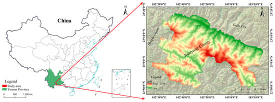
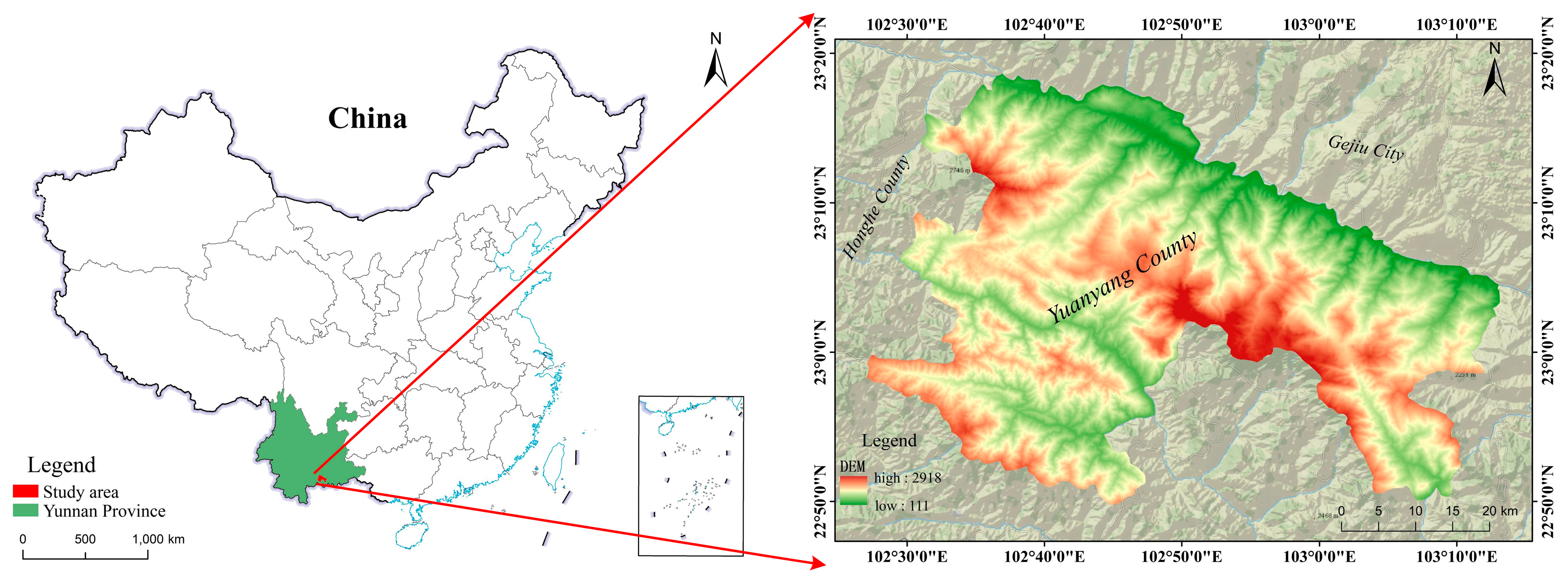
The study area is located in Yuanyang County, Yunnan Province, spanning 102°27′03″E–103°13′11″E and 22°49′41″N–23°18′37″N. It covers ~2212.32 km2, extending 55 km north–south and 74 km east–west. Nansha Town (the county seat) is 284 km from Kunming and 71 km from Mengzi, adjacent to Jinping County (south), Honghe/Lüchun Counties (west), and Jianshui County/Gejiu City (north, across the Yuanjiang River). Situated in the southern Ailaoshan Mountains, the area features a typical middle-mountain deeply incised terrain with high mountains, deep valleys, and abrupt slopes. Intensively eroded by the Yuanjiang (north) and Tengtiao River (south) systems, the terrain slopes northwest–southeast with V-shaped gorges. The northwest–southeast trending Guanyinshan Mountains divide the county into two parts, forming the watershed between the two rivers. With slopes generally >20° (59.1% of the area > 25°), the region has a striking elevation difference: 111 m (lowest) to 2918 m (highest), with a relative relief of 2807 m and fragmented terrain. The location of the study area is shown in Figure 1.
Figure 1.
Location of Yuanyang County in Yunnan Province.
2.2. Data Sources and Preprocessing
2.2.1. Multi-Source Geospatial Data
The data used in this study include three categories: (1) Sentinel-1 and Sentinel-2 satellite images provided by the European Space Agency (ESA); (2) High-resolution multi-source fused digital orthophoto images, covering domestic and commercial high-resolution satellite data such as BJ-2 (Beijing-2), GF-2 (Gaofen-2), GJ-1 (Gaojing-1), and WorldView-2/3 (WV-2/3); (3) Physical geography data, including topographic, meteorological, and other basic environmental data.
The sources and relevant attributes of each type of data are shown in Table 1.
Table 1.
Data types and sources.
To ensure the consistency and comparability of subsequent analyses, all spatial data were uniformly processed: the spatial resolution was resampled to 10 m, and the coordinate system was uniformly converted to the CGCS2000_3_Degree_GK_CM_102E projected coordinate system. Notably, while the satellite imagery and meteorological data were strictly synchronized with the 2019 growing season, the topographic data (DEM) represents a stable long-term baseline. We assume that these terrain features are stationary over a decadal scale; thus, the temporal gap between the DEM and the 2019 observations is considered to have a negligible impact on crop identification.
2.2.2. Crop Phenological Data
Crop phenological information plays a crucial role in remote sensing classification. It can not only effectively distinguish crop types with similar spectral characteristics but different growth rhythms, but also provide guidance for the optimal selection of multi-temporal remote sensing images. Based on regional agricultural production knowledge, historical agricultural statistical data, and relevant literature, this study compiled a typical phenological calendar for major crops (e.g., rice, maize) in the study area, and conducted temporal calibration for key growth stages of these crops (e.g., sowing, tillering/jointing, maturity). As shown in Table 2, the phenological calendar clearly presents the growth rhythm characteristics of major crops within different time windows, providing an important a priori basis for subsequent crop identification, phenological change monitoring, and classification feature extraction based on multi-temporal remote sensing images.
Table 2.
Phenological Stages of Major Crops in Yuanyang.
3. Research Methods
3.1. Overall Research Framework
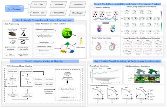
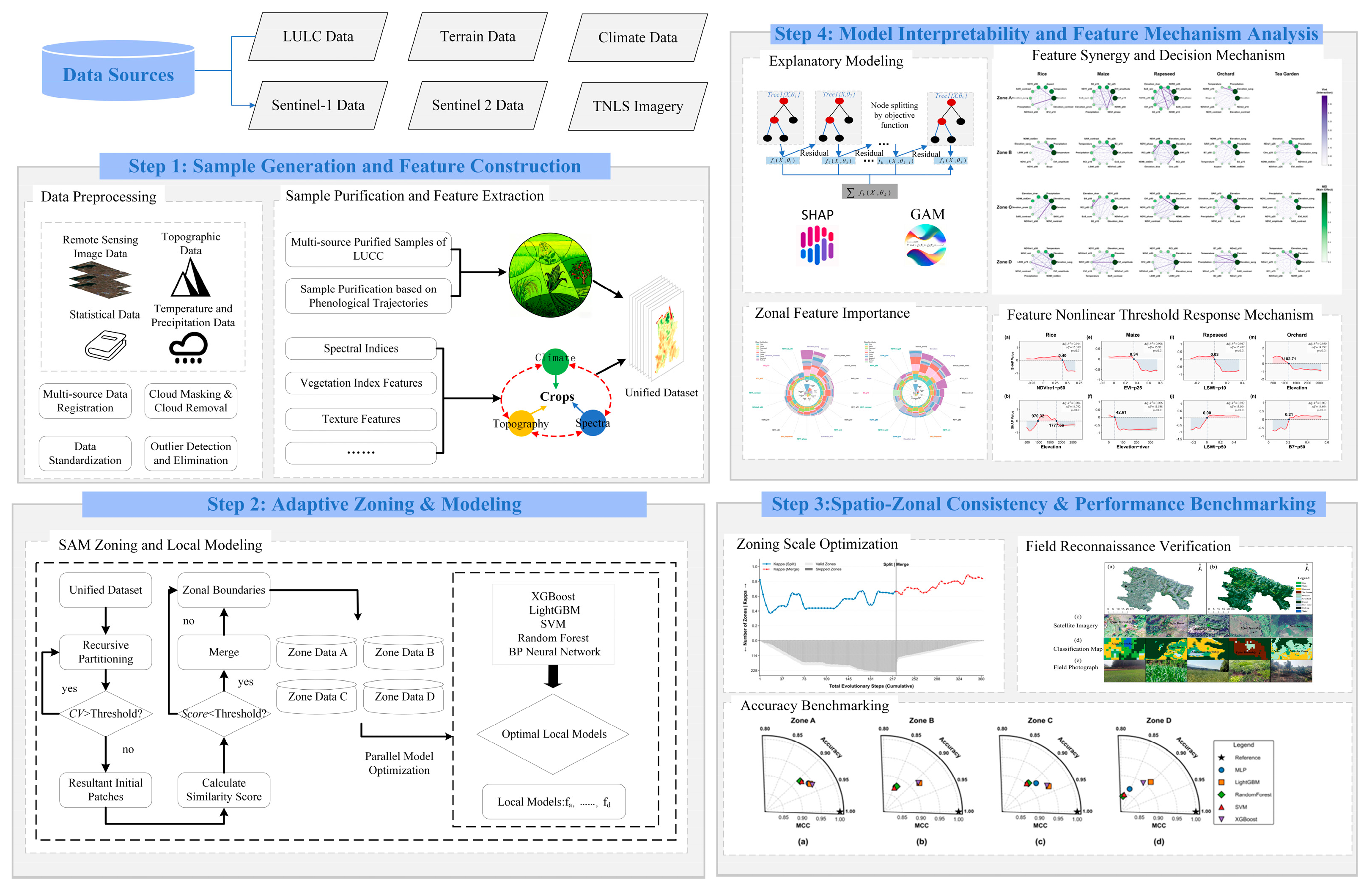
The technical framework of this study is illustrated in Figure 2 and comprises four main stages. First, a unified multi-temporal remote sensing dataset was constructed by integrating multi-source data, including Sentinel-1/2, terrain, and climate data. Crop and non-crop samples were generated based on purified Land Use/Land Cover (LULC) samples and phenological curves, around which a multi-dimensional feature set incorporating spectral, texture, topographic, and meteorological features was built. Second, an adaptive geographic zoning algorithm was applied to partition the study area into spatially homogeneous subregions. Within each partition, multiple local models (e.g., XGBoost, Random Forest) were independently trained and evaluated to identify the optimal classifier for each zone. Third, spatio-zonal consistency and performance stability were evaluated. This stage involved analyzing the relationship between partitioning granularity and classification accuracy to determine the optimal scale of spatial stationarity. The reliability of the localized models was assessed through k-fold cross-validation, and the final mapping results were further validated using independent field reconnaissance data to ensure real-world accuracy. Finally, to ensure model interpretability, methods such as SHAP (version 0.47.1) and GAMs (pyGAM version 0.10.1) were integrated to reveal the model’s internal decision-making processes and the crop–environment interaction mechanisms, examining dimensions such as feature synergy, the spatial differentiation of feature importance, and nonlinear responses.
Figure 2.
The framework of crop identification in the study. (Step 1) Multi-source data integration, preprocessing, and multi-dimensional feature construction; (Step 2) adaptive spatial zoning based on recursive partitioning and local classification modeling; (Step 3) zoning scale optimization, field verification, and accuracy benchmarking; (Step 4) model interpretability analysis and feature response mechanism.
3.2. Spatial Zoning Strategy and Experimental Configuration
3.2.1. SAM Adaptive Geospatial Zoning Algorithm
To address geospatial non-stationarity in large-scale remote sensing classification—manifested as global model degradation due to the “same object, different spectra” and “different objects, same spectra” phenomena—this study proposes a fully data-driven adaptive geospatial zoning algorithm based on the Spectral Angle Mapper (SAM)–derived Classification Confusion Index. The method requires no prior knowledge, fixed windows, or manual zoning, and partitions heterogeneous regions into spatially homogeneous subregions through a top-down splitting and bottom-up merging framework.
During top-down splitting, spectral homogeneity within each zone is evaluated using the spectral coefficient of variation (CV), a dimensionless statistic widely adopted in image segmentation for homogeneity assessment and internal spectral dispersion characterization [12,13]. Zones are recursively subdivided until predefined homogeneity, sample size, or depth constraints are met. For a given region, CV is defined as:
where represents the standard deviation (dispersion) and the mean (average level). In the algorithm, CV is computed for each band, and the mean across all bands is used as the final evaluation metric.
The centroids of the final homogeneous subregions are extracted as seed points, from which an initial zoning scheme is generated using Voronoi tessellation, providing a stable spatial structure for subsequent merging.
Bottom-up merging is applied to mitigate over-segmentation and enhance geographical coherence. To quantify spectral similarity between adjacent zones, the Spectral Angle Mapper (SAM) [14] was selected. Unlike traditional distance-based metrics such as Euclidean Distance (ED), which measures the magnitude of spectral differences, SAM measures the angle between spectral vectors [15,16]. This is a critical distinction in plateau mountainous regions where terrain-induced shadows create significant brightness (amplitude) disparities for identical crop types. While ED is sensitive to these amplitude shifts—often leading to fragmentation driven by illumination rather than biological phenology—SAM isolates the spectral shape (curve trend) from brightness [17,18]. This capability effectively transforms the “same object, different spectra” problem caused by shadows into a consistent vector similarity, ensuring that phenological patterns remain stable across complex terrains [19,20,21]. The SAM angle is calculated as follows:
where denotes the spectral angle between zones and , and represents the high-dimensional vector of band-wise mean values; smaller angles indicate greater similarity.
To incorporate spatial context, a unified similarity score is constructed by integrating normalized spectral distance and spatial adjacency, following widely adopted spectral–spatial classification strategies in remote sensing studies [22,23]:
where and are preset spectral and spatial weights (0.8 and 0.2 in this study), is the normalized spectral distance, and is the spatial adjacency distance.
The normalized spectral distance is calculated as:
Values closer to 0 indicate higher spectral similarity and a greater likelihood of consistent land cover types. The spatial adjacency distance is defined as:
where denotes the shared boundary length, and and are the total perimeters of the respective zones. This formulation ensures that merged zones maintain good spatial compactness.
Merging is conducted in two stages: (1) global optimal merging based on an adaptive similarity threshold derived from adjacent zone pairs, establishing the primary zoning structure; and (2) residual merging, in which small or sample-deficient zones are merged with their most similar neighbors until minimum size constraints are satisfied. The final zoning system exhibits high spectral homogeneity and spatial compactness, providing a robust basis for subsequent local modeling.
3.2.2. Parameter Justification and Computational Environment
To ensure the scientific rigor, reproducibility, and robustness of the adaptive zoning and local modeling framework, the selection of key parameters and the computational infrastructure are justified as follows:
- (1)
- Zoning Parameters: We set the CV threshold () to 0.35 after testing (0.1–0.5), balancing patch homogeneity against geospatial non-stationarity. The minimum sample size () was fixed at 200 pixels to ensure statistical stability during 5-fold cross-validation. The recursion depth () was capped at 8 to align with the regional average patch size () and optimize throughput.
- (2)
- Spatial Regularization: A weight ratio of 4:1 was applied between spectral () and spatial () components. This configuration emphasizes phenological characteristics while ensuring geographical compactness and mitigating “salt-and-pepper” effects.
- (3)
- Hardware/Software: Data preprocessing was conducted via Google Earth Engine. Local computations utilized an Intel i5-12600KF CPU and an NVIDIA RTX 4060 GPU for high-speed spatial processing and SHAP-based model interpretation. For the study area (~2212.32 km2), the total execution time of the proposed framework—encompassing the SAM-based adaptive partitioning and the training of all localized classifiers—was approximately 2.5 h.
3.3. Local Modeling Method Construction
After completing the SAM-based adaptive zoning, a local classification model is constructed for each sub-region respectively to enhance crop identification performance in complex mountainous environments. Let the spatial position be denoted as s, with the corresponding feature vector as x(s); the study area is divided into several spatial sub-regions, denoted as {S1, S2,…, Sn}. A local training set is built for each sub-region:
On this basis, the training objective of the local model fk is to minimize:
where L is the loss function, and Ω is the regularization term for spatial local complexity. The model aims to minimize the classification error within the region, enabling the learner to have local adaptability.
For samples near regional boundaries, their spatial positions may be close to multiple sub-regions. Thus, Inverse Distance Weighting (IDW) is adopted to fuse the outputs of multiple local models, achieving smoother and more continuous cross-regional prediction results.
The set of neighboring local models is defined as:
where ck is the center of region Rk.
The distance is defined as:
The IDW weight is defined as:
The final prediction expression for boundary samples is:
This strategy ensures the continuity and smoothness of cross-regional prediction results, effectively avoiding the issue of abrupt boundary changes.
3.4. Model Benchmarking and Performance Evaluation
To identify the optimal crop classification model for complex plateau mountain environments and establish a unified benchmark for local zoning, five representative classifiers are evaluated: Support Vector Machine (SVM), Random Forest (RF), XGBoost, LightGBM, and Multi-Layer Perceptron (MLP). SVM constructs a maximum-margin hyperplane and excels in high-dimensional, small-sample scenarios. RF, a Bagging ensemble, enhances robustness through multi-tree voting. XGBoost (version 1.7.5) and LightGBM (version 3.3.5), based on Boosting, sequentially learn residuals, with LightGBM employing GOSS and EFB for improved efficiency on large datasets. MLP leverages multi-layer nonlinear mappings to capture complex relationships between remote sensing features and land cover classes.
To assess the effectiveness of the SAM-driven adaptive partitioning, three modeling scenarios were compared: (1) a global baseline using the unified sample pool without partitioning; (2) a random partitioning baseline where samples were arbitrarily divided into four groups; and (3) a rule-based topographic baseline using fixed elevation intervals (<1000 m, 1000–1600 m, 1600–2200 m, and >2200 m). To ensure an impartial comparison, all models across these scenarios utilized an identical 194-dimensional feature set. Hyperparameters were independently optimized using a grid-search strategy with 5-fold cross-validation, ensuring that performance gains are attributable to the partitioning logic rather than sub-optimal tuning.
Model performance was quantified using Overall Accuracy (OA), the Kappa coefficient, and the Matthews Correlation Coefficient (MCC). The MCC was prioritized to evaluate robustness against class imbalance inherent in fragmented agricultural landscapes. This multi-scenario benchmarking identifies the model with the highest generalization capability, forming the basis for subsequent local modeling and interpretability analysis.
3.5. Model Interpretability Analysis Methods
As a nonparametric extension of the generalized linear model (GLM), the generalized additive model (GAM) flexibly captures complex nonlinear relationships between variables by incorporating nonparametric smoothing functions, such as splines or local regression [24]. Unlike traditional linear regression, GAM estimates each smoothing function via the backfitting algorithm, automatically adapting predictor forms without prespecifying functional structures [25]. Moreover, its additive structure ensures that the contributions of individual explanatory variables to the response are independent and additive, substantially enhancing model interpretability [26]. The model can be expressed as:
where the link function is set as the identity function, denotes the smoothing function based on thin-plate regression splines, and is a Gaussian random error term.
To identify key environmental factors and spectral features influencing crop classification [27], this study employs the SHapley Additive exPlanations (SHAP) method [28]. SHAP quantifies the contribution of each environmental variable and spectral feature to crop distribution predictions. Based on cooperative game theory, SHAP decomposes model outputs into the marginal contributions of individual features, enabling a quantitative understanding of the model’s decision-making process. For a given sample and input feature , the Shapley value is defined as:
where is the full feature set, is a subset excluding feature , and represents the independent contribution of feature to the prediction for sample . By calculating the Shapley value for each feature, SHAP quantifies their individual contributions to the final classification results, revealing the model’s decision logic at the feature level and transforming it from a “black box” into a “white box”.
4. Results and Analysis
4.1. Zoning Results
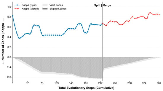
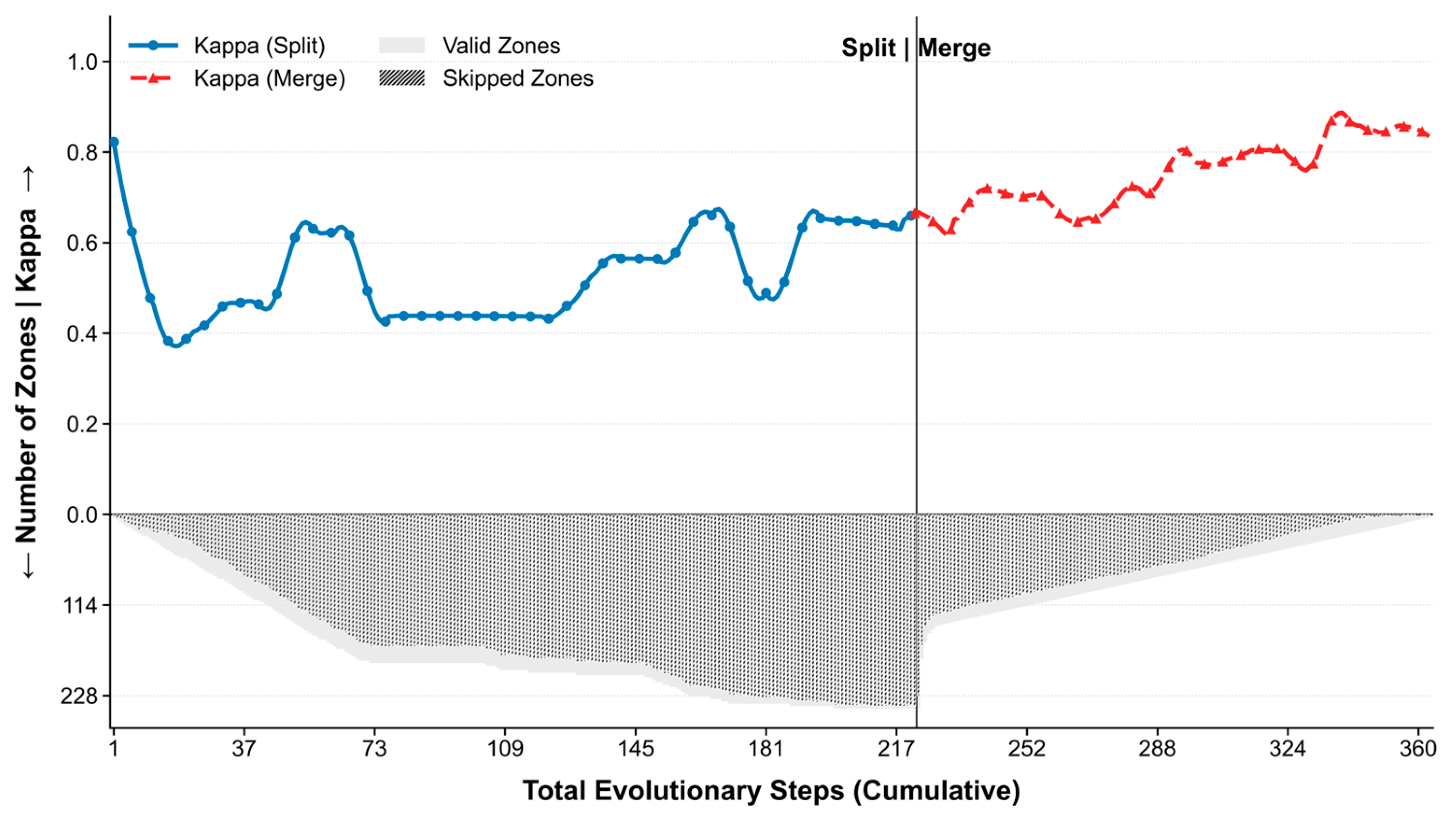
Optimal partitioning intensity was determined using an evolutionary “Split-Merge” process, balancing partitioning intensity against local model robustness (Figure 3).
Figure 3.
Dynamics of Kappa Coefficient and Partition Evolution during Adaptive Zoning. Y-axis arrows indicate the increasing directions for the Kappa coefficient (upward) and the number of zones (downward).
During the Split phase (steps 1–225), the feature space was over-decomposed. The prevalence of Skipped Zones (grey bars) indicated that many partitions were unable to support effective training due to insufficient sample size. This coincided with the unstable and sub-optimal performance of the Kappa coefficient (blue curve), confirming that over-partitioning compromises model generalization.
The subsequent Merge phase (steps 226–360) systematically consolidated these weak units. The Kappa coefficient (red curve) exhibited a monotonic improvement, ultimately converging on an optimal configuration of four zones. This final configuration reflects a data-optimized trade-off, maximizing intra-zonal biophysical homogeneity while ensuring the sample sufficiency required for robust local modeling.
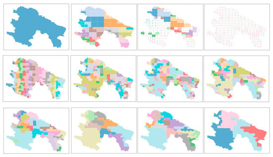
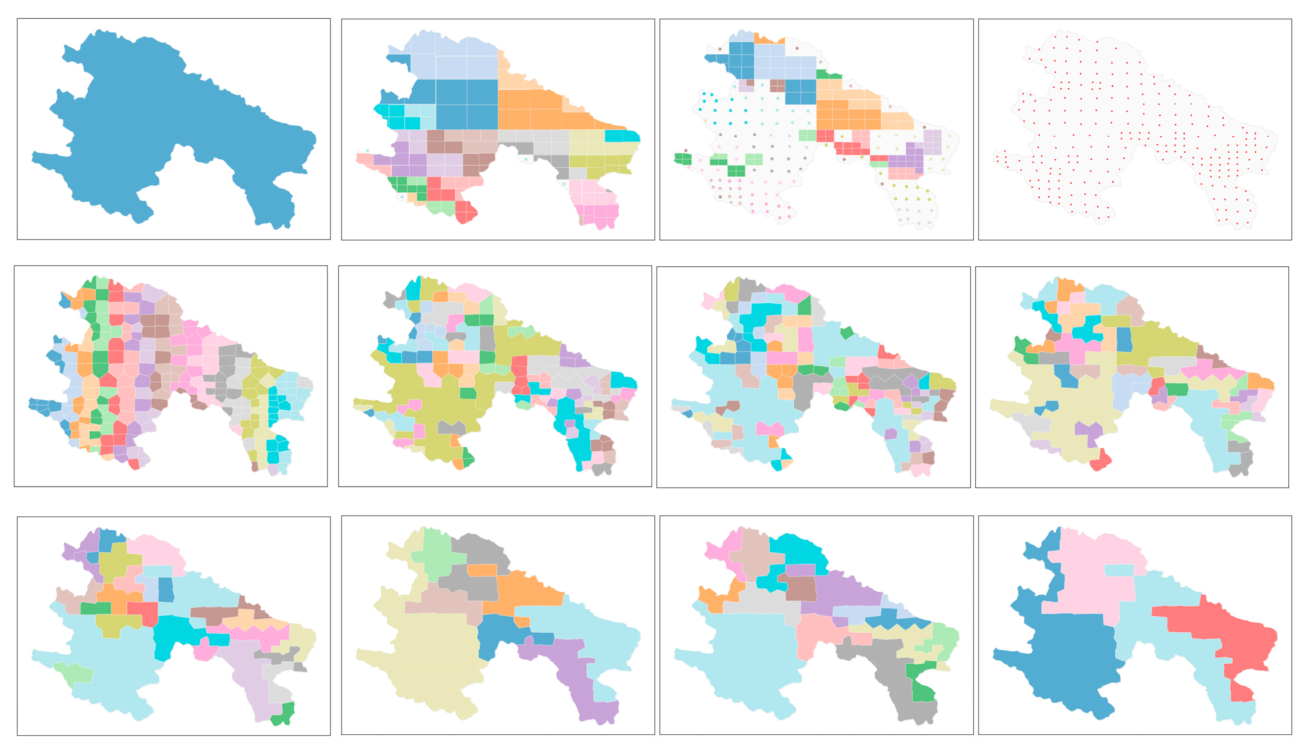
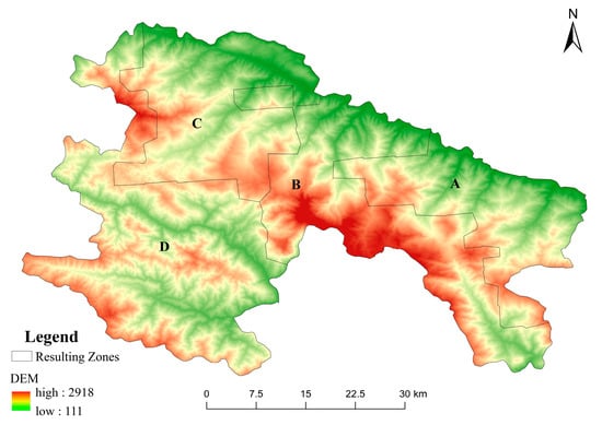
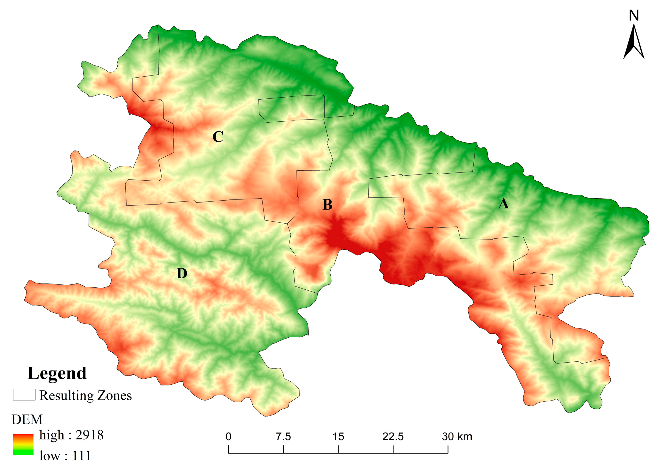
Figure 4 delineates the iterative evolution of the adaptive zoning process across 12 sequential stages, illustrating the step-wise transition from initial global partitioning to final convergence. Each sub-panel represents a refinement step of the “Split-Merge” algorithm, where the SAM-based clustering progressively optimizes the boundaries to maximize intra-zonal biophysical homogeneity. This iterative refinement ultimately resulted in 4 optimized geospatial zones. These zones demonstrate significant spatial structural coherence rather than a stochastic distribution, exhibiting high alignment with regional topographic features and environmental gradients (Figure 5).
Figure 4.
Schematic Diagram of Zoning Process.
Figure 5.
Overlay of the partitioning results on the elevation map. Labels A–D denote the identified study zones.
Zone A (Dam/Basin—Foothill Zone): Mainly distributed in the blue and light green areas in the DEM, indicating low-elevation valley dams, basins, and gentle foothill slopes. With open and flat terrain, it is a typical low-elevation surface concentrated with agricultural activities.
Zone B (Ridge—Peak Highland): Scattered in the central and southern parts of the study area, covering the red elevation areas in the DEM in the form of “island-like patches”, representing mountain tops and main ridge lines. This zone features large topographic relief and steep slopes, showing typical alpine geomorphic characteristics.
Zone C (Alpine to River Valley Transition Zone): Occupying the eastern, northeastern, and northern peripheral areas of the study area, it forms an arc-shaped transition zone at medium-low elevations. It has a large elevation range, transitioning from the medium-high elevation slopes adjacent to Zone B to the low-elevation river valleys in the northeast. This zone reflects the extensive slope system transitioning from alpine regions to outer river valleys.
Zone D (Core Plain and River Valley Agricultural Zone): Located in the central part of the study area, it has flat terrain, favorable light and irrigation conditions, and serves as a typical high-yield agricultural core area.
In general, the SAM zones have clear topographic gradient significance, forming a complete gradient of geomorphology and agricultural systems from mountain tops to slopes, transition zones, and plains. This geographical differentiation provides a reliable basis for the subsequent construction of local models sensitive to spatial heterogeneity.
4.2. Dataset Construction and Classification Performance Evaluation
4.2.1. Feature Dataset Construction
Taking Yuanyang County, a representative agricultural county in Yunnan, as the study area, this research constructed a high spatiotemporal density, multi-source remote sensing feature dataset covering the entire annual growing season. Data sources included 169 Sentinel-2 optical images, processed with strict time-series cloud removal via QA60/SCL dual masking, and 101 Sentinel-1 SAR images, selected to ensure meteorologically independent time-series continuity.
From these datasets, 10 original spectral bands and 16 derived indices were extracted to characterize vegetation greenness, canopy moisture, and red-edge signatures. These indices include NDVI, EVI, NDWI, Cire, NDre1, NDre2, NDVIre1, NDVIre2, NDVIre3, SAVI, GNDVI, NDMI, NDRE, LSWI, RCI, and NDYI. To capture intra-annual temporal dynamics, five percentiles (10th, 25th, 50th, 75th, and 90th) were calculated for each band and index from the annual time series. Additionally, four radar features—VV and VH polarizations, the Polarization Ratio (PR: VH/VV), and Total Power (TP: VV+VH)—were integrated.
Multi-source auxiliary data were incorporated, encompassing topographic parameters (elevation, slope, and aspect). To characterize spatial structural heterogeneity across multiple dimensions, texture features were extracted using the Gray-Level Co-occurrence Matrix (GLCM) from three distinct base layers: Elevation, NDVI, and SAR backscatter. Specifically, 16 GLCM statistics (including Contrast, Correlation, Angular Second Moment, Entropy, and Dissimilarity) were calculated for the Elevation layer. In contrast, for the NDVI and SAR layers, although eight common GLCM features were initially evaluated, a parsimonious set of three conceptually distinct core descriptors—Contrast, Correlation, and Entropy—was ultimately selected for each (six features in total). This selection was made to minimize information overlap and ensure model parsimony. All texture metrics were computed using a 3 × 3 moving window and 64 quantization levels, with values averaged across 16 directions to ensure rotation invariance. Furthermore, we integrated climatic indicators (annual total precipitation and mean maximum temperature) and dynamic metrics (annual standard deviation of key indices, EVI peak amplitude/date, and EVI area under the curve (AUC)).
The final dataset consists of a 194-dimensional multi-modal raster feature set, comprehensively characterizing surface properties across spectral, structural, phenological, textural, topographic, and climatic dimensions. Additionally, 1 m-resolution fused high-resolution images and annual land use change data provided by the Yuanyang County Bureau of Natural Resources served as reference data, offering high-precision land cover spatial structure and functioning as an authoritative benchmark for classification accuracy assessment.
4.2.2. Model Accuracy Evaluation and Optimization Analysis
To validate the effectiveness of the proposed strategy, the dataset was partitioned into a training set (80%) and an independent test set (20%). A 5-fold cross-validation was applied to the training set for hyperparameter optimization. The Matthews Correlation Coefficient (MCC) and Overall Accuracy (OA) were jointly adopted as evaluation metrics to ensure a balanced assessment of multi-class performance and overall classification reliability.
Table 3 summarizes the classification results of the five models based on the global dataset. Overall, LightGBM achieved the highest performance across all four evaluation metrics (OA, Kappa, F1, MCC), significantly outperforming traditional machine learning algorithms. XGBoost ranked second, with performance closely approaching that of LightGBM, highlighting the inherent advantages of the gradient boosting framework in handling high-dimensional, multi-modal remote sensing features.
Table 3.
Global Model Classification Results.
In comparison, although MLP demonstrates strong nonlinear fitting capability, its performance was slightly lower than ensemble learning methods, likely due to sensitivity to sample size and hyperparameter settings. SVM and Random Forest exhibited limited ability to capture detailed spectral information in multi-class, high-heterogeneity scenarios, resulting in comparatively lower accuracy.
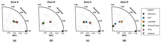
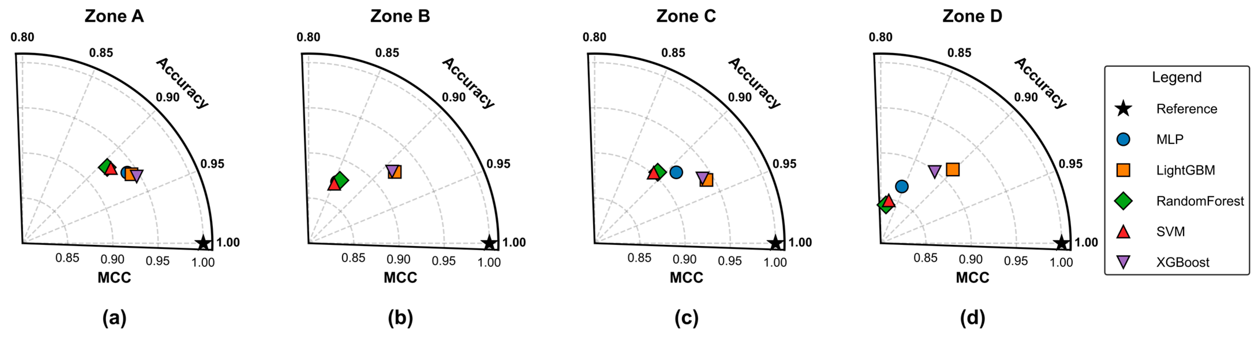
Based on SAM-based geographical partitioning, this study further trained and validated the five models within four sub-regions (A, B, C, and D), as illustrated in Figure 6. The evaluation results are summarized as follows:
Figure 6.
Taylor Diagrams of OA and MCC for Zones A–D (a–d). The black star denotes the ideal reference (1.0, 1.0). Proximity to the reference star indicates superior model performance in terms of both accuracy and consistency.
Region A (gentle terrain with high spectral separability): The classification difficulty was the lowest, and all models achieved relatively high overall accuracy. Among them, XGBoost performed the best (OA = 0.946, MCC = 0.933), slightly exceeding LightGBM (OA = 0.943, MCC = 0.930).
Region B (ridge crests with strong heterogeneity): Severe spectral mixing and category interleaving increased classification difficulty. Nevertheless, LightGBM maintained high accuracy (OA = 0.924, MCC = 0.912), demonstrating stronger robustness.
Region C (alpine-valley transition zone): Within this transition zone, LightGBM (OA = 0.942, MCC = 0.934) and XGBoost (OA = 0.939, MCC = 0.931) performed higher than the other candidate models.
Region D (core agricultural plain, strongly affected by surface humidity): Spectral differences decreased, but LightGBM achieved the highest metrics among the evaluated algorithms (OA = 0.914, MCC = 0.903).
Compared to the global model, LightGBM demonstrated the highest overall consistency, achieving an average OA of 0.931 and MCC of 0.920. Although XGBoost showed a marginal advantage in the topographically simple Region A, LightGBM was more robust in complex, heterogeneous terrains (Regions B, C, and D). To ensure analytical consistency and a reliable foundation for subsequent feature interpretability analysis across all sub-regions, LightGBM was selected as the unified core algorithm.
To conclusively demonstrate that the performance gains are specifically attributable to the SAM-driven partitioning (S4), a comparison against the Global Baseline (S1) and two alternative zoning strategies (S2: Random; S3: Rule-based Topographic) was conducted. As shown in Table 4, S4 achieved the highest overall performance (OA: 93.1%). Crucially, Random Partitioning (S2, OA: 83.1%) performed significantly worse than the Global Baseline (S1, OA: 91.9%). This experimental hierarchy () validates two key findings: (1) arbitrary partitioning degrades model robustness by imposing artificial boundaries; and (2) the performance gain is specifically attributed to SAM’s ability to maximize intrinsic feature homogeneity by utilizing a physics-informed similarity metric.
Table 4.
Performance comparison of different partitioning strategies.
Overall, the results indicate that SAM-based geographical partitioning substantially improved model performance and clearly outperformed the global modeling approach. Partitioned modeling effectively mitigated geospatial non-stationarity, enhanced classification consistency and generalization, and thus represents a more effective strategy for crop identification in mountainous regions.
4.2.3. Field Survey Verification
To complement the internal validation, an independent external validation was conducted through systematic field campaigns in representative townships. A stratified random sampling strategy was employed to select a total of 364 validation points. These points were proportionally allocated across major land cover classes and were strategically selected to cover diverse geomorphic units and planting scenarios, including terraces, sloping farmland, dedicated cash crop zones, and heterogeneous mixed land cover areas. The ground truth for each point was rigorously determined using a high-precision GPS receiver, supplemented by on-site observation, UAV imagery, and a “map–image–ground” tripartite comparison against high-resolution reference imagery.
An independent validation confusion matrix was generated by comparing these ground-truthed points against our classification map. The results indicate a high degree of agreement, achieving an Overall Accuracy (OA) of 94.2% and a Kappa coefficient of 0.92. These external metrics are consistent with the internal cross-validation performance, confirming the model’s strong generalization capability.
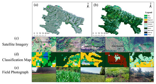
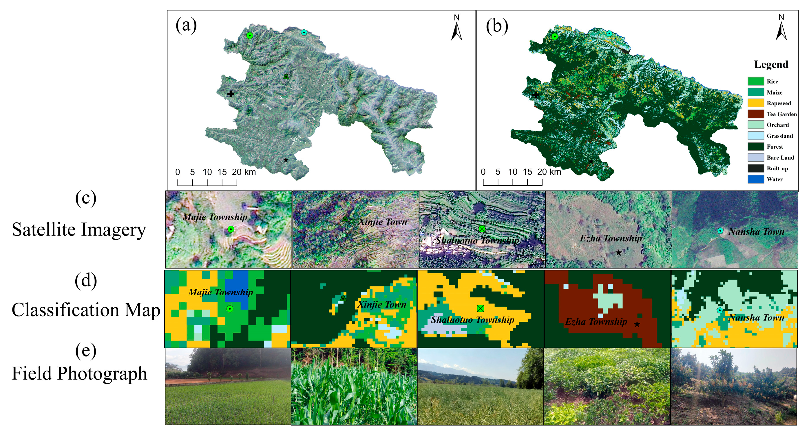
In addition to the quantitative metrics, a qualitative assessment was performed to evaluate the model’s spatial consistency. As illustrated in Figure 7, the classification maps exhibit high consistency with actual ground conditions, even in challenging mountainous environments. For instance, the model identified terrace rice and dryland Maize in Majie and Xinjie Townships, with classification textures corresponding to high-resolution image features. In Esha and Nansha Townships, it also delineated cash crops, such as tea gardens and grapefruit orchards, from surrounding vegetation with clear boundaries.
Figure 7.
Comparison between classification results and ground-truth validation. (a,b) Overview of high-resolution satellite imagery and the produced classification map for the study area. (c–e) Zoomed-in comparison for five typical sites, displaying high-resolution satellite imagery, classification results, and corresponding field photographs in rows from top to bottom.
In summary, the field validation, which combined a quantitative assessment with a qualitative inspection of typical areas, provides independent support for the reliability of the classification results. The findings indicate that the classification framework maintains stable recognition capabilities under complex and heterogeneous real-world conditions, establishing a data foundation for subsequent agricultural monitoring.
4.3. Spatial Differentiation Analysis of Feature Importance
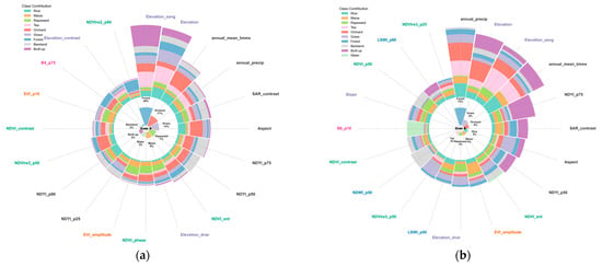
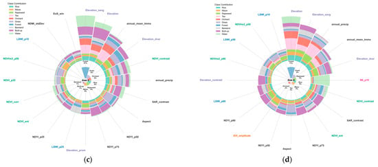
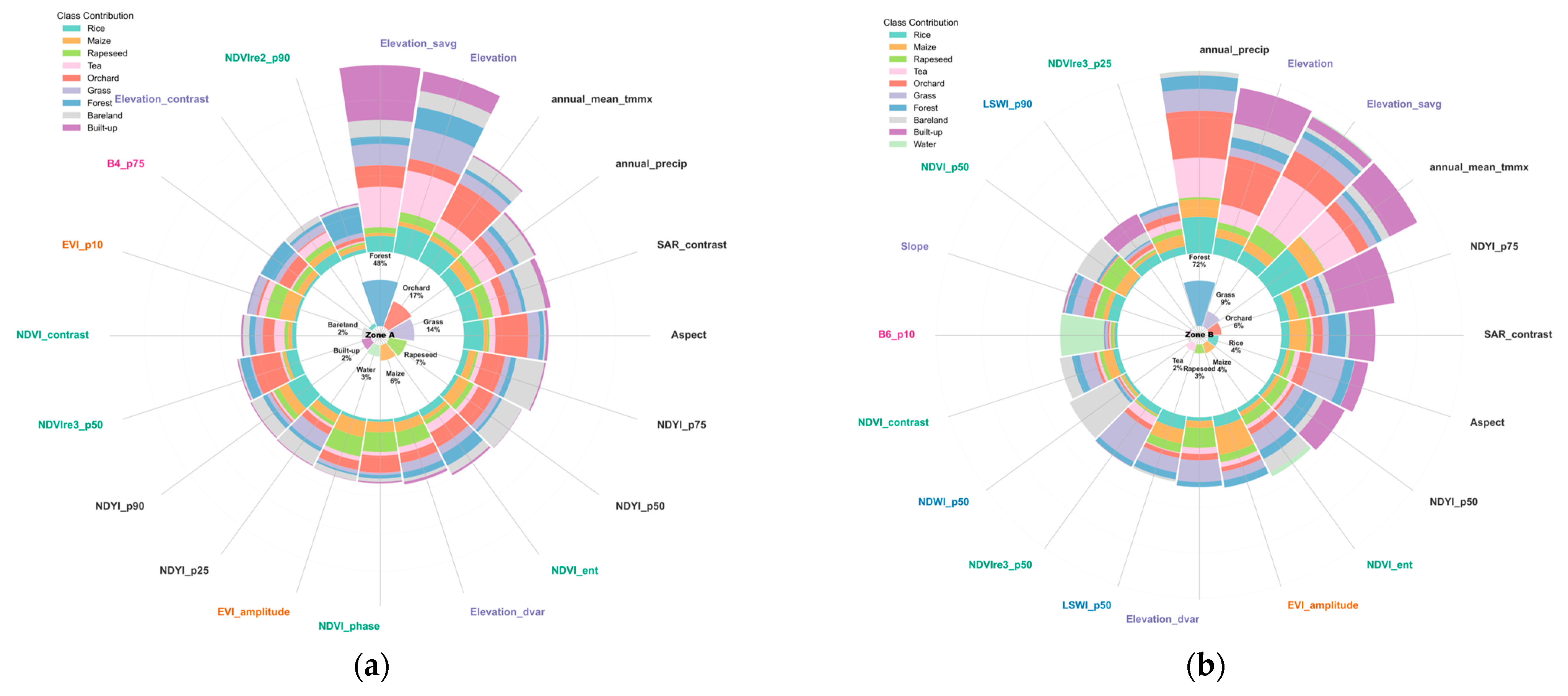
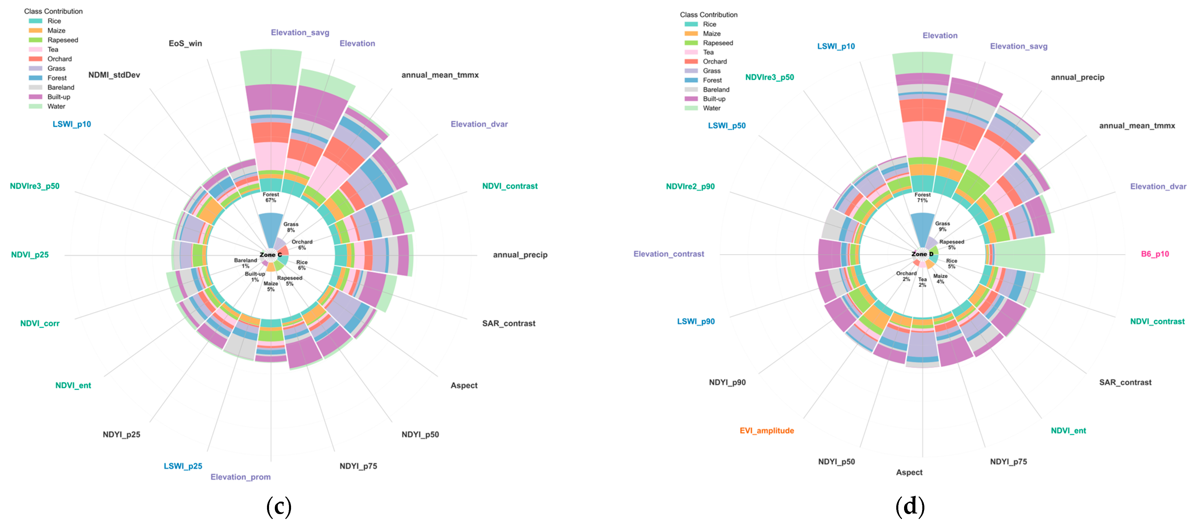
To reveal the geospatial non-stationarity of remote sensing classification in complex mountainous environments, this study systematically analyzed feature dependence patterns of major crops using SHAP values derived from partitioned LightGBM models (Figure 8). The results indicate that although topographic factors (e.g., elevation) exert a general influence at the global scale, the recognition mechanisms of major crops vary significantly across different geographical partitions, exhibiting pronounced spatial heterogeneity. This is particularly evident for rice (104.09 km2), Maize (100.12 km2), and rapeseed (110.37 km2).
Figure 8.
Spatial heterogeneity of SHAP feature importance across partitions. (a) Zone A, (b) Zone B, (c) Zone C, and (d) Zone D.
Partition A: Plain and Basin Area—Microtopography + SAR Texture-Dominated Mechanism (Figure 8a)
Covering 197.33 km2, this region is a major concentration of rapeseed (14.35 km2) and Maize (11.17 km2). Key model features include elevation, aspect, and SAR texture (contrast), which effectively capture subtle topographic undulations and differences in crop canopy roughness in flat areas. The importance of radar texture in this partition exceeds that in other areas, highlighting its sensitivity in gently undulating terrain and its unique value for fine-scale agricultural classification.
Partition B: Plateau and Hilly Area—Climate-Dominated Mechanism (Figure 8b)
With an area of 309.06 km2, this region is characterized by strong topographic variability and high forest coverage. Although crop areas are relatively small, the model exhibits a distinct decision-making pattern: annual average maximum temperature emerges as the most critical feature, surpassing topographic factors. Rice (11.28 km2), Maize (11.25 km2), and rapeseed (9.40 km2) occupy similar zones. Due to significant local microclimate differences induced by slope position, the model primarily distinguishes thermophilic crops (e.g., Maize) from cold-tolerant crops (e.g., rapeseed) through temperature gradients. This climate-dominated mechanism is less pronounced in partitions with more stable terrain.
Partition C: Alpine-Valley Transition Zone—Terrain + Climate Synergistic Mechanism (Figure 8c)
As the largest partition (930.31 km2) and the core agricultural area, it has the widest crop distribution: rice (55.89 km2), rapeseed (48.95 km2), and Maize (43.15 km2). The model forms a composite mechanism driven by elevation, topographic variability, and climate factors (temperature). Terrain guides the identification of suitable rice growth areas such as river valleys and plains, while climate helps exclude arid crops with spectral characteristics similar to rice. This mechanism effectively addresses complex scenarios of spectral mixing and crop intermingling typical of large-scale transition zones.
Partition D: Plain-Valley Zone—Spectrum (B6−p10) + Precipitation-Dominated Mechanism (Figure 8d)
Covering 772.67 km2, main crops include rice (36.15 km2), rapeseed (37.67 km2), and Maize (34.55 km2). The model’s decision-making structure here differs markedly from other partitions: the low percentile of shortwave infrared band B6 (B6−p10) is the core feature for detecting rice flooding phenology, while precipitation acts as a critical auxiliary variable, regulating differences between dryland and paddy systems. B6−p10 effectively captures the weak water spectral reflection of rice during early flooding, significantly improving rice recognition accuracy.
The patterns of feature attribution across Partitions A to D exhibit a systematic gradient in model decision logic: model predictions in Partition A are primarily associated with microtopography and SAR texture, Partition B shows a higher sensitivity to climate factors, Partition C integrates synergistic terrain and climate features, and Partition D is influenced significantly by spectral signals (rice flooding signals) and precipitation. These results illustrate that partitioned models can effectively capture the spatially varying influence of features (geospatial non-stationarity) in remote sensing classification, which global models struggle to represent. Therefore, local models provide a more nuanced attribution of regional characteristics, which is critical for enhancing accuracy and robustness in mountainous crop classification.
4.4. Feature Synergy and Decision-Making Mechanism Analysis
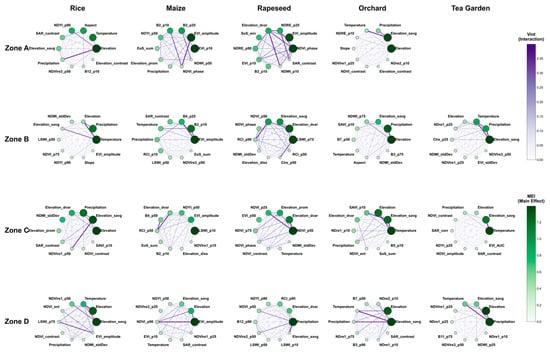
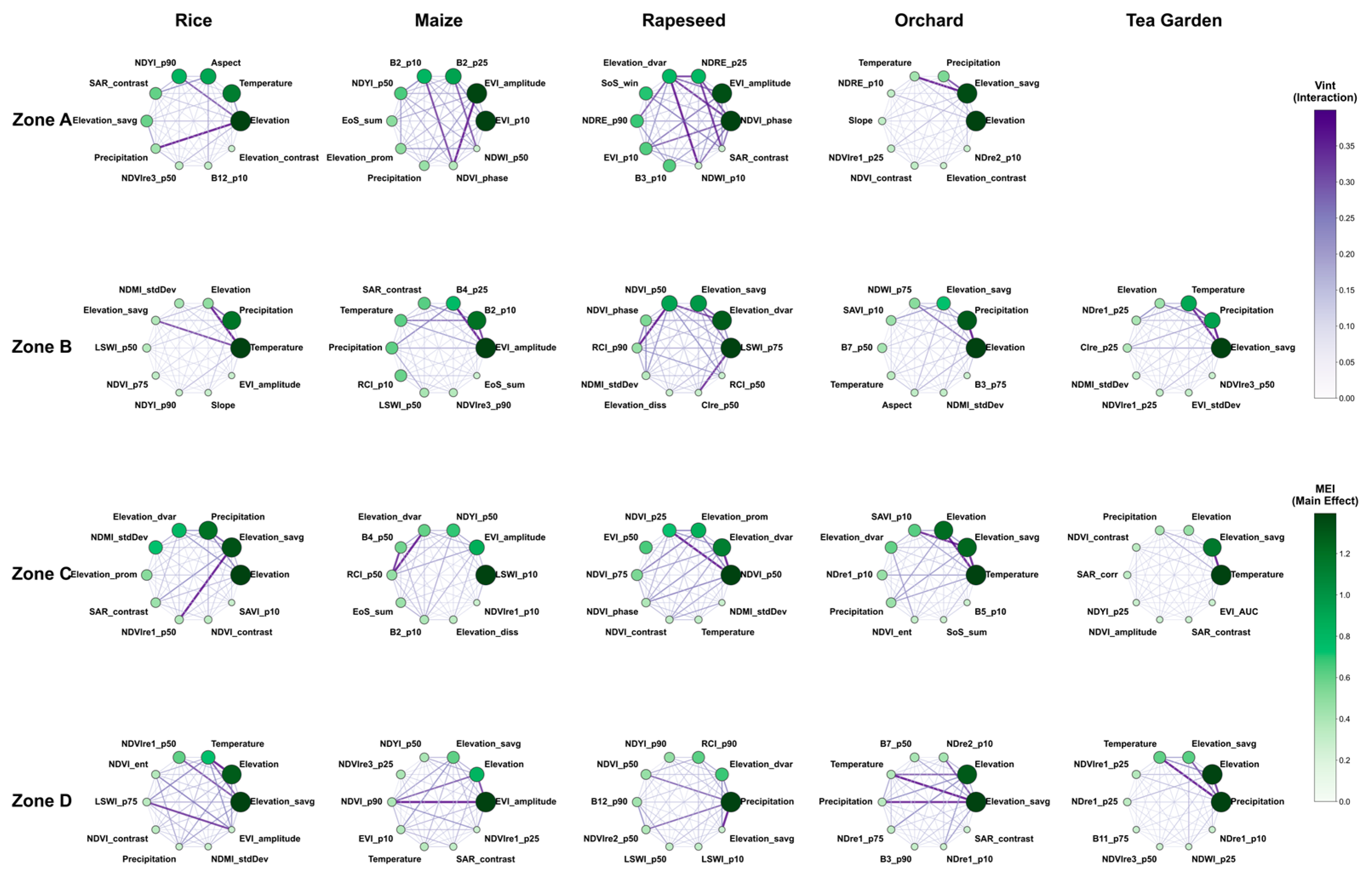
To further dissect the internal decision-making mechanisms of the local models, this study constructed a SHAP-based feature interaction network across different zones and crop types (Figure 9). In this network, each node represents a specific feature, with its size and green-scale intensity indicating the Main Effect Index (MEI)—the independent contribution of that feature to the model. The edges connecting the nodes represent the interaction effects (), where line thickness and purple-scale intensity reflect the synergistic strength between feature pairs. Based on these visualizations, we introduced two key concepts—the “feature synergy paradigm” and the “decision weight trade-off”—to deconstruct the discriminative logic of the models.
Figure 9.
Network visualization of Main Effect Importance (MEI) and Variable Interaction effects (Vint) for crop models in each partition.
The feature synergy paradigm refers to the optimized combination of features learned by the model to maximize class separability. While a fundamental “terrain + phenology” synergy exists across all zones for initial screening, local models develop specialized paradigms adapted to regional conditions. For instance, in Zone A, a prominent “hydrological-topographic” synergy (e.g., Elevation and Precipitation) is crucial for rice identification, reflecting the dual environmental constraints of water availability and terrain. In Zone D, the network reveals a tightly coupled “spectral-hydrological-topographic” synergy (comprising SWIR, water indices, and elevation), forming an exclusive paradigm for the precise identification of paddy fields in valley environments.
The decision weight trade-off describes the model’s adaptive redistribution of feature importance in response to varying geographic contexts. In the relatively gentle terrain of Zone A, the model accentuates radar texture (e.g., SAR−contrast), shifting its focus to microstructural information to compensate for diminished topographic gradients. Conversely, in the complex terrains of Zones B and C, the model reduces reliance on potentially noisy radar signals in favor of more stable macro-topographic and climatic features. This dynamic adjustment demonstrates the model’s ability to “trade off” weights to maintain robust performance across heterogeneous landscapes.
Compared with global models, which often suffer from a “homogenization constraint” that dilutes region-specific feature signals, the partitioned local models independently construct optimal discriminative logic. This approach achieves a form of “geographic intelligence”: emphasizing texture in plains, climate in mountainous areas, and specific spectral-hydrological signals in river valleys. By doing so, local models successfully bridge the gap between local optimality and global adaptability.
4.5. Nonlinear Threshold Response Mechanism of Feature Recognition
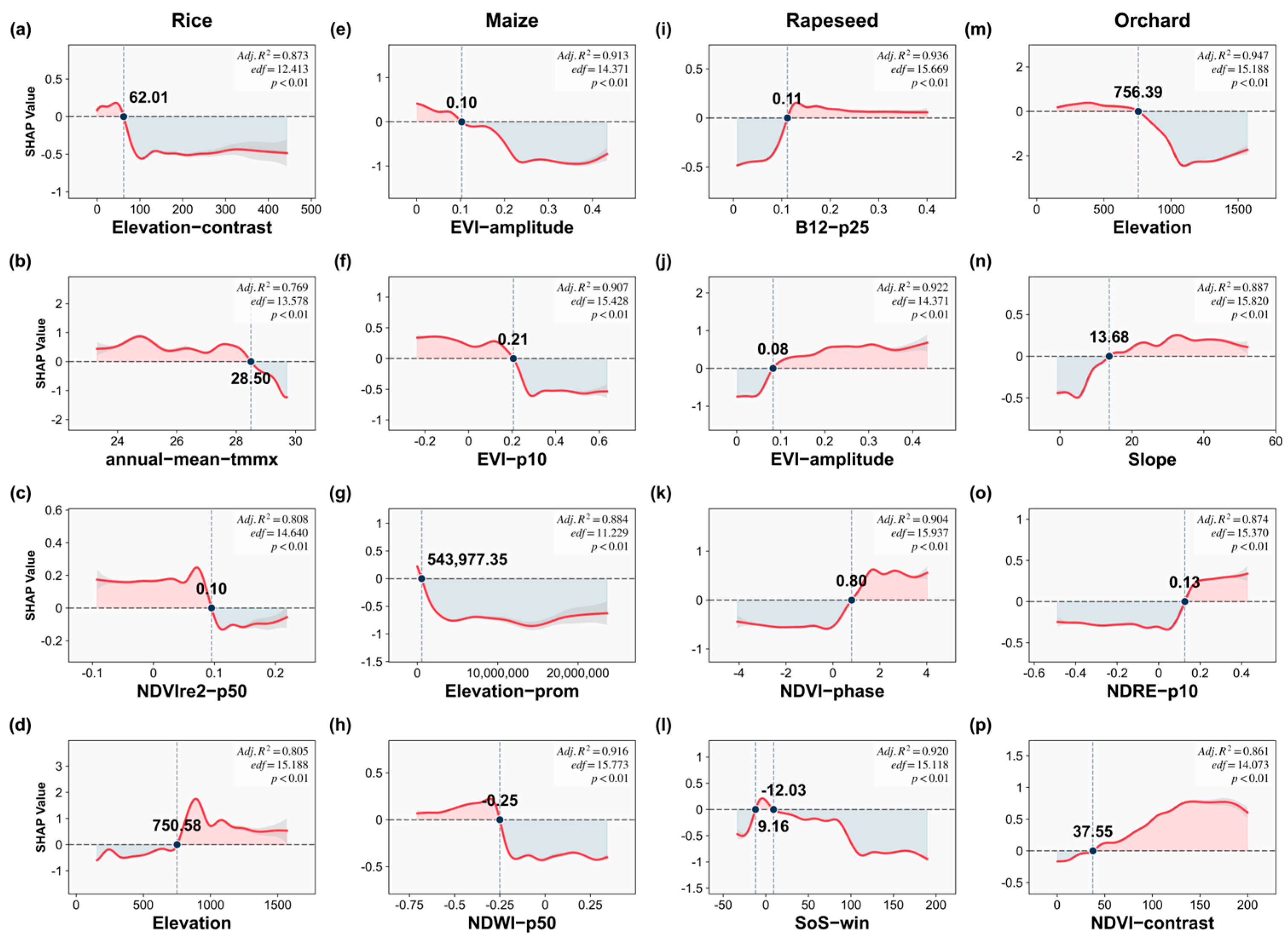
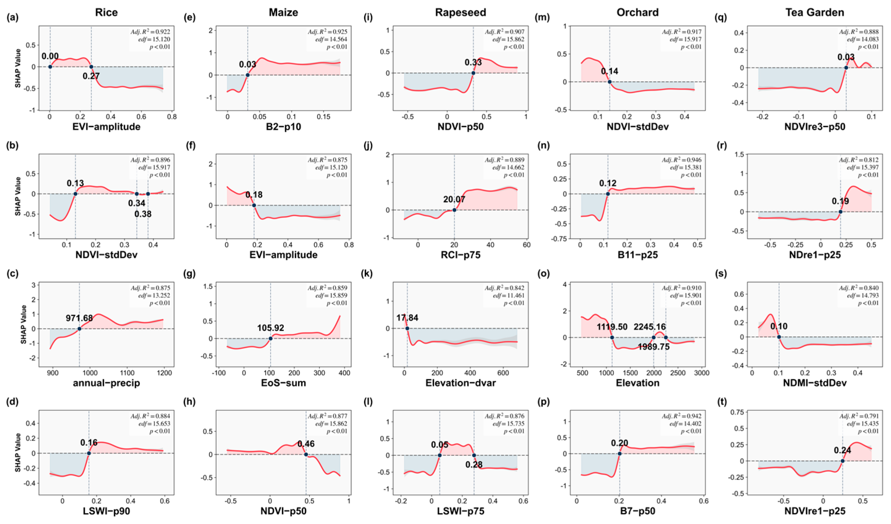
To investigate nonlinear threshold effects in crop identification, GAMs combined with SHAP values were applied to five major crops: rice, maize, rapeseed, orchards, and tea gardens. This approach revealed abrupt changes in feature importance when key environmental thresholds were crossed, highlighting complex crop–environment interactions.
In Partition A (Plain Area), the “Microtopography-Dominated Pattern” drives crop segregation. Rice exhibits distinct “thermal avoidance,” confined to flat areas with moderate temperatures (<28.5 °C; Figure 10b). Dryland crops are distinguished by specific spectral traits: Maize is characterized by its sensitivity to low EVI amplitudes (Figure 10e), while Orchards are identified via high NDRE values (Figure 10o) and high texture contrast (Figure 10p). These features effectively distinguish the complex canopies of orchards from uniform field crops. Furthermore, the specific elevation constraints (Figure 10m) and the absence of Tea confirm the model’s adherence to macro-scale topographical limitations.
Figure 10.
Non-linear response curves and threshold analysis for key features in the classification of major crops in Zone A. Panels (a–d) correspond to Rice; (e–h) Maize; (i–l) Rapeseed; (m–p) Orchard. Red-shaded and blue-shaded background regions signify positive (SHAP > 0) and negative (SHAP < 0) influence zones, respectively.
Partition B (Plateau-Hilly Area) exhibits a distinct “Environmental Stress-Adaptive Pattern.” Rice shows a pronounced “hydrological dependency,” with SHAP values turning positive when annual precipitation exceeds 971.68 mm (Figure 11c) and LSWI−p90 is above 0.16 (Figure 11d). Maize adapts to specific phenological and spectral windows, characterized by an EVI−amplitude < 0.18 (Figure 11f) and a delayed end of the growing season (EoS−sum > 105.92, Figure 11g). Perennial crops display clear vertical zonality: Tea Gardens rely heavily on high-altitude red-edge features, particularly when NDVIre3−p50 > 0.03 (Figure 11q) and NDre1−p25 > 0.19 (Figure 11r). In contrast, Orchards occupy specific elevation zones, showing a positive contribution primarily at elevations below 1119.50 m (Figure 11o).
Figure 11.
Non-linear response curves and threshold analysis for key features in the classification of major crops in Zone B. Panels (a–d) correspond to Rice; (e–h) Maize; (i–l) Rapeseed; (m–p) Orchard; and (q–t) Tea Garden. Red-shaded and blue-shaded background regions signify positive (SHAP > 0) and negative (SHAP < 0) influence zones, respectively.
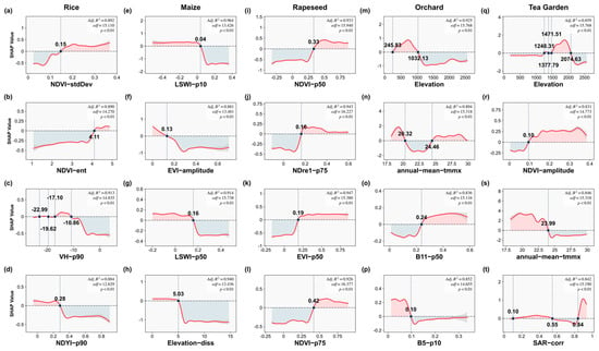
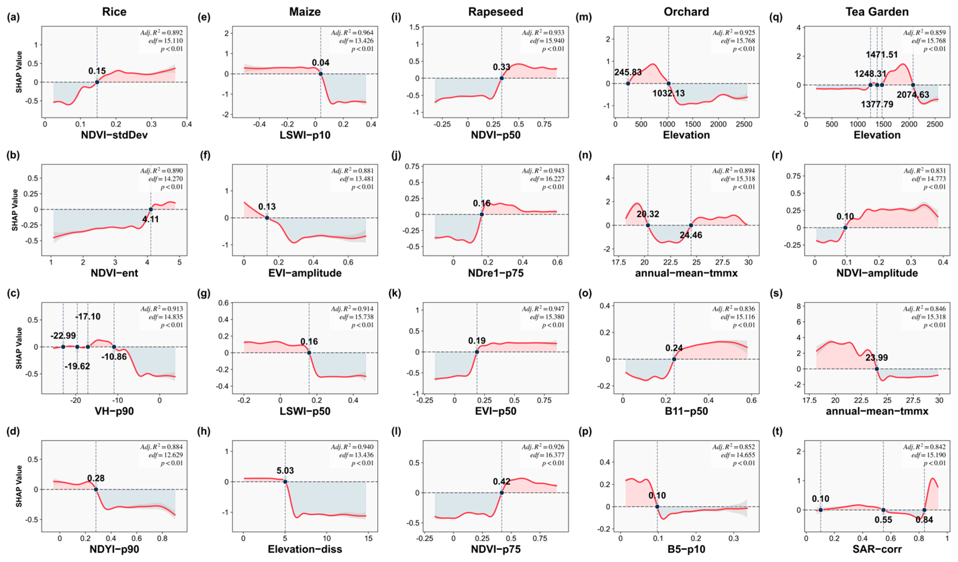
Partition C (Slope Transition Zone) follows a “Gradient Response Pattern” that clearly separates annual from perennial crops. Annual crops (Rice/Maize) are regulated by seasonal dynamics; for instance, Rice responds positively to higher intra-season NDVI variability (NDVI−stdDev > 0.15, Figure 12a), whereas Maize is more suited to areas with lower EVI amplitude (EVI−amplitude < 0.13, Figure 12f). Conversely, perennials are constrained by long-term topographic and climatic conditions. Orchards and Tea Gardens occupy distinct elevation niches: Orchards show peak suitability in a “mid-slope” zone between 245 m and 1032 m in elevation (Figure 12m), while Tea Gardens are concentrated at significantly higher altitudes from 1248 m to 2074 m (Figure 12q). This distinct vertical stratification, with orchards occupying an intermediate elevation between low-lying croplands and high-altitude tea plantations, directly illustrates the region’s multi-layered agricultural landscape.
Figure 12.
Non-linear response curves and threshold analysis for key features in the classification of major crops in Zone C. Panels (a–d) correspond to Rice; (e–h) Maize; (i–l) Rapeseed; (m–p) Orchard; and (q–t) Tea Garden. Red-shaded and blue-shaded background regions signify positive (SHAP > 0) and negative (SHAP < 0) influence zones, respectively.
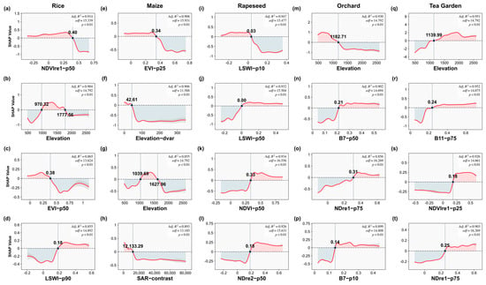
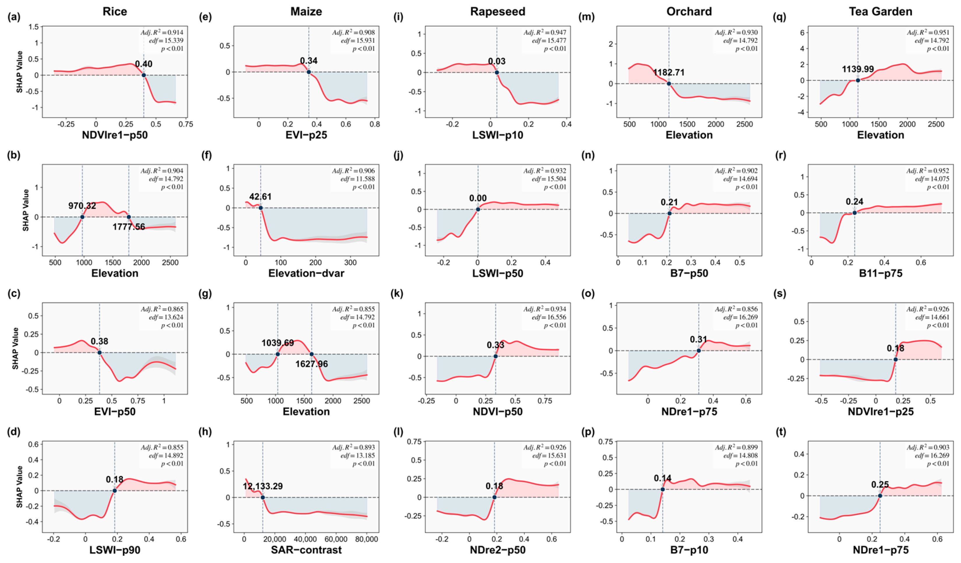
Partition D (Core Plain Area) reveals an “Irrigation and Micro-topographic Pattern.” Rice distribution is defined by artificial moisture availability, with its suitability increasing significantly when LSWI−p90 exceeds 0.18 (Figure 13d). Maize, in contrast, is adapted to more homogeneous terrain, showing a positive contribution in areas with low topographic variation (Elevation−dvar < 42.61, Figure 13f). Notably, even within this generally flat landscape, Orchards and Tea Gardens are sharply restricted to localized, “island-like” highlands. Orchards exhibit a sharp positive response to elevations above 1182.71 m (Figure 13m), while Tea Gardens show a similar dependency on elevations greater than 1139.99 m (Figure 13q). This demonstrates the model’s sensitivity to micro-geomorphology, where subtle elevation changes within the plain create the specific micro-drainage conditions critical for perennial cultivation.
Figure 13.
Non-linear response curves and threshold analysis for key features in the classification of major crops in Zone D. Panels (a–d) correspond to Rice; (e–h) Maize; (i–l) Rapeseed; (m–p) Orchard; and (q–t) Tea Garden. Red-shaded and blue-shaded background regions signify positive (SHAP > 0) and negative (SHAP < 0) influence zones, respectively.
5. Discussion
5.1. Method Effectiveness and Mechanism Analysis
The proposed framework effectively mitigates the performance degradation inherent in global modeling by explicitly addressing geospatial non-stationarity. Unlike conventional models that enforce a uniform decision boundary across heterogeneous terrains, adaptive partitioning transforms a high-variance feature space into biophysically consistent subspaces, thereby alleviating the “homogenization constraint” that often suppresses local signal sensitivity [29,30].
- (1)
- Local Modeling and Variance Reduction: The efficacy of local modeling (Table 3) is rooted in the mitigation of the “same object, different spectra” paradox. By utilizing Spectral Angle Mapper (SAM) for partitioning, the framework prioritizes spectral vector direction over absolute magnitude, effectively neutralizing the radiometric distortions caused by topographic shading. This data-driven partitioning enables local classifiers to resolve subtle phenological variations that would otherwise be obscured by the global variance of a unified dataset. This spatial subdivision logic is consistent with the adaptive partitioning strategy proposed by Zhou and Duan, who demonstrated that localized data handling can effectively neutralize spatial errors in global topographic products [31]. This mechanism addresses the limitations of distance-based zoning by focusing on intrinsic material properties rather than extrinsic illumination conditions [32].
- (2)
- Mechanistic Interpretation of Decision Logic: The observed “decision weight trade-off” (Section 4.4) reflects a systematic shift in environmental drivers across different landscape units. In highlands (Zones B/C), the model prioritizes hydro-topographic variables, capturing the physiological limits of crops along vertical gradients. In plains (Zones A/D), the logic shifts toward spectral-texture synergy to differentiate crops with overlapping spectral profiles but distinct canopy structures. The identified thresholds (e.g., the 28.5 °C thermal limit and 971 mm precipitation boundary) align with established agrometeorological principles, confirming that the model has internalized physical geographic rules rather than spurious statistical correlations [33,34].
- (3)
- Complementarity of Multi-Source Information: The multi-source synergy is driven by the invariance of radar texture to illumination conditions. While optical data are susceptible to topographic effects, SAR backscatter provides stable structural information regarding canopy roughness. According to the critical review by Samadzadegan et al., the synergy of multi-sensor and multi-platform data is essential for resolving the high spatial heterogeneity inherent in complex landscapes [35]. Furthermore, metrics such as NDMI standard deviation capture seasonal hydrological rhythms (e.g., flooding processes), transitioning the task from static spectral mapping to dynamic process detection. This integration is consistent with the theoretical shift toward multi-sensor fusion in complex landscapes, where single-source data are insufficient to resolve high spatial heterogeneity [36].
5.2. Research Limitations
Despite the promising outcomes in methodological design and mechanistic analysis, this study has several limitations that warrant further investigation:
- (1)
- Conflict between Discrete Zoning Boundaries and Continuity of Geographic Processes: Adaptive zoning produces discrete spatial boundaries, whereas real-world geographic processes—such as climatic gradients and vegetation transitions—are continuous. This can create boundary effects in ecological transition zones, where edge samples may be assigned to mismatched units, potentially affecting continuity and stability of identification results.
- (2)
- Mixed Pixel Issue Arising from Complex Planting Patterns: Relay intercropping and mixed cropping systems are common in the study area. At Sentinel-2’s 10 m resolution, spectral signals often represent combinations of multiple crops, causing phenological curve aliasing and reducing the model’s ability to distinguish typical crop spectra.
- (3)
- Stability and Optimality of the Zoning Algorithm: The thresholds used in our zoning algorithm were determined empirically for this study area. The stability of these partitions with respect to minor changes in input data, and the transferability of the algorithm’s parameters to different geographical contexts, warrant further investigation.
5.3. Future Outlook
To further enhance the model’s generalization capability, spatial adaptability, and geographic consistency, future research may focus on the following directions:
- (1)
- Extending from Discrete Zoning to Continuous Gradient Modeling: Future research could explore fuzzy membership, continuous spatial weights, or kernel-smoothed zoning to better represent continuous geographic gradients, reducing boundary effects and improving applicability in transition zones.
- (2)
- Extending from Pixel-level Classification to Sub-pixel Multi-scale Fusion Analysis: integrating spectral mixture analysis, fractional coverage models, and UAV-based high-resolution data can address mixed-pixel issues, capture finer land cover structures, and further enhance classification accuracy and stability.
6. Conclusions
This study demonstrates that local modeling based on adaptive geographic partitioning provides a robust solution for crop identification in plateau mountainous regions. By systematically mitigating the errors induced by geospatial non-stationarity, the proposed framework achieved an overall accuracy (OA) of 93.1% and a Kappa coefficient of 0.919, significantly outperforming conventional global modeling baselines.
The substantive findings and significance are as follows:
- (1)
- Methodological Insight: The effectiveness of the framework is derived from the use of SAM-based partitioning, which decouples spectral morphology from topographic illumination variance. This reduction in intra-zonal heterogeneity allows the model to capture subtle phenological signatures that are typically suppressed in global datasets. A key finding is that intra-zonal biophysical consistency is more critical for classification accuracy than the absolute volume of training samples, suggesting that “targeted learning” is superior to “massive learning” in complex terrains.
- (2)
- Scientific Insight: Feature contribution analysis reveals that the drivers of crop identification are spatially non-stationary. High-altitude identification is primarily constrained by hydrothermal thresholds (e.g., <28.5 °C thermal limit for maize and >971 mm precipitation for rice), while low-altitude areas rely on the synergy between spectral response and radar texture. These quantified thresholds provide empirical evidence for crop–environment interactions, transitioning remote sensing from statistical mapping to the discovery of rule-based geographic knowledge.
- (3)
- Practical Significance: The identified biophysical limits and spatial rules provide a quantitative foundation for agricultural zoning and crop suitability assessment in Yuanyang County. This study offers a scalable approach for high-precision food security monitoring in topographically complex regions where standard global models exhibit significant performance degradation.
Subsequent research should address the representation of transition zones by incorporating continuous gradient modeling to replace discrete boundaries. Additionally, integrating sub-pixel decomposition techniques will be essential to resolve persistent mixed-pixel challenges in extreme mountainous landscapes.
Author Contributions
Conceptualization, G.C. and Z.S.; methodology, G.C.; validation, G.C. and C.W.; formal analysis, J.Z. and Y.W. (Yandong Wang); investigation, G.C.; writing—original draft preparation, G.C.; writing—review and editing, G.C. and J.Z.; supervision, J.Z.; project administration, G.C. and W.L.; funding acquisition, Z.S. and Y.W. (Yanying Wang). All authors have read and agreed to the published version of the manuscript.
Funding
This research was funded by the National Natural Science Foundation of China, grant number 42561066; the Yunnan Major Science and Technology Projects and Key R&D Program, grant number 202403ZC380001; the Ministry–Province Cooperation Project on Natural Resources, grant numbers No. 2247 and 2024ZRBSHZ095; the Yunnan Philosophy and Social Science Planning Project, grant number ZX2024YB59; the Kunming Science and Technology Program, grant number 2025-NS-003; and the Open Fund of the Yunnan Key Laboratory of Intelligent Monitoring and Spatiotemporal Big Data Governance for Natural Resources, grant number 202449CE340023.
Data Availability Statement
The original contributions presented in this study are included in the article. Further inquiries can be directed to the corresponding author.
Conflicts of Interest
Author Yandong Wang was employed by the company Yunnan Yunjindi Technology Co., Ltd., and author Changman Wang was employed by the company Yunnan Jiaotou Ecological Environment Engineering Co., Ltd. The remaining authors declare that the research was conducted in the absence of any commercial or financial relationships that could be construed as a potential conflict of interest.
References
- Zheng, Y.; Dong, W.; Yang, Z.; Lu, Y.; Zhang, X.; Dong, Y.; Sun, F. A new attention-based deep metric model for crop type mapping in complex agricultural landscapes using multisource remote sensing data. Int. J. Appl. Earth Obs. Geoinf. 2024, 134, 104204. [Google Scholar] [CrossRef] [Scilit]
- Tian, X.; Chen, Z.; Li, Y.; Bai, Y. Crop Classification in Mountainous Areas Using Object-Oriented Methods and Multi-Source Data: A Case Study of Xishui County, China. Agronomy 2023, 13, 3037. [Google Scholar] [CrossRef] [Scilit]
- Fang, G.; Wang, C.; Dong, T.; Wang, Z.; Cai, C.; Chen, J.; Liu, M.; Zhang, H. A Landscape-Clustering Zoning Strategy to Map Multi-Crops in Fragmented Cropland Regions Using Sentinel-2 and Sentinel-1 Imagery with Feature Selection. Agriculture 2025, 15, 186. [Google Scholar] [CrossRef] [Scilit]
- Kyere, I.; Astor, T.; Graß, R.; Wachendorf, M. Agricultural crop discrimination in a heterogeneous low-mountain range region based on multi-temporal and multi-sensor satellite data. Comput. Electron. Agric. 2020, 179, 105864. [Google Scholar] [CrossRef] [Scilit]
- Ren, T.; Xu, H.; Cai, X.; Yu, S.; Qi, J. Smallholder Crop Type Mapping and Rotation Monitoring in Mountainous Areas with Sentinel-1/2 Imagery. Remote. Sens. 2022, 14, 566. [Google Scholar] [CrossRef] [Scilit]
- Zhao, J.; Zhong, Y.; Hu, X.; Wei, L.; Zhang, L. A robust spectral-spatial approach to identifying heterogeneous crops using remote sensing imagery with high spectral and spatial resolutions. Remote Sens. Environ. 2020, 239, 111605. [Google Scholar] [CrossRef] [Scilit]
- Zhang, J.; Wu, T.; Luo, J.; Hu, X.; Wang, L.; Li, M.; Lu, X.; Li, Z. Toward Agricultural Cultivation Parcels Extraction in the Complex Mountainous Areas Using Prior Information and Deep Learning. IEEE Trans. Geosci. Remote Sens. 2025, 63, 1–14. [Google Scholar] [CrossRef] [Scilit]
- Xiao, L.; Wang, J.; Yang, K.; Zhou, H.; Meng, Q.; He, Y.; Shen, S. SE-ResUNet Using Feature Combinations: A Deep Learning Framework for Accurate Mountainous Cropland Extraction Using Multi-Source Remote Sensing Data. Land 2025, 14, 937. [Google Scholar] [CrossRef] [Scilit]
- Yang, R.; Qi, Y.; Zhang, H.; Wang, H.; Zhang, J.; Ma, X.; Zhang, J.; Ma, C. A Study on the Object-Based High-Resolution Remote Sensing Image Classification of Crop Planting Structures in the Loess Plateau of Eastern Gansu Province. Remote Sens. 2024, 16, 2479. [Google Scholar] [CrossRef] [Scilit]
- Liu, L.; Yang, J.; Yin, F.; He, L. High-Resolution Mapping of Maize in Mountainous Terrain Using Machine Learning and Multi-Source Remote Sensing Data. Land 2025, 14, 299. [Google Scholar] [CrossRef] [Scilit]
- Zhang, H.; Wang, Y.; Shang, J.; Liu, M.; Li, Q. Investigating the impact of classification features and classifiers on crop mapping performance in heterogeneous agricultural landscapes. Int. J. Appl. Earth Obs. Geoinf. 2021, 102, 102388. [Google Scholar] [CrossRef] [Scilit]
- Sang, Y.; Gu, H.; Meng, Q.; Men, X.; Sheng, J.; Li, N.; Wang, Z. An evaluation of the performance of remote sensing indices as an indication of spatial variability and vegetation diversity in alpine grassland. Remote Sens. 2024, 16, 4726. [Google Scholar] [CrossRef] [Scilit]
- Rossi, C.; Kneubuehler, M.; Schuetz, M.; Schaepman, M.E.; Haller, R.M.; Risch, A.C. Spatial resolution, spectral metrics and biomass are key aspects in estimating plant species richness from spectral diversity in species-rich grasslands. Remote Sens. Ecol. Conserv. 2022, 8, 297–314. [Google Scholar] [CrossRef] [Scilit]
- Kruse, F.A.; Lefkoff, A.B.; Boardman, J.W. The spectral image processing system (SIPS)—Interactive visualization and analysis of imaging spectrometer data. Remote Sens. Environ. 1993, 44, 145–163. [Google Scholar] [CrossRef] [Scilit]
- Van der Meer, F. The effectiveness of spectral similarity measures for the analysis of hyperspectral imagery. Int. J. Appl. Earth Obs. Geoinf. 2006, 8, 3–17. [Google Scholar] [CrossRef] [Scilit]
- Sohn, Y.; Rebello, N.S. Supervised and unsupervised spectral angle classifiers. Photogramm. Eng. Remote Sens. 2002, 68, 1271–1280. [Google Scholar]
- Riaño, D.; Chuvieco, E.; Salas, J.; Aguado, I. Assessment of different topographic corrections in Landsat-TM data for mapping vegetation types. IEEE Trans. Geosci. Remote Sens. 2003, 41, 1056–1061. [Google Scholar] [CrossRef] [Scilit]
- Mazer, A.; Martin, M.; Lee, M.; Solomon, J. Image processing software for imaging spectrometry data analysis. Remote Sens. Environ. 1988, 24, 201–210. [Google Scholar] [CrossRef] [Scilit]
- Bargiel, D. A new method for crop classification combining time series of radar images and crop phenology information. Remote Sens. Environ. 2017, 198, 369–383. [Google Scholar] [CrossRef] [Scilit]
- Rowan, L.C.; Mars, J.C. Lithologic mapping in the Mountain Pass, California area using Advanced Spaceborne Thermal Emission and Reflection Radiometer (ASTER) data. Remote Sens. Environ. 2003, 84, 350–366. [Google Scholar] [CrossRef] [Scilit]
- Chang, C.-I. An information-theoretic approach to spectral variability, similarity, and discrimination for hyperspectral image analysis. IEEE Trans. Inf. Theory 2000, 46, 1927–1932. [Google Scholar] [CrossRef] [Scilit]
- Wang, L.; Shi, C.; Diao, C.; Ji, W.; Yin, D. A survey of methods incorporating spatial information in image classification and spectral unmixing. Int. J. Remote Sens. 2016, 37, 3870–3910. [Google Scholar] [CrossRef] [Scilit]
- Chen, S.; Zhang, H.; Sun, T.; Zhao, J.; Guo, X. Remote sensing image classification using the spectral-spatial distance based on information content. Sensors 2018, 18, 3428. [Google Scholar] [CrossRef] [Scilit]
- Long, H.; Zhang, Y.; Ma, L.; Tu, S. Land use transitions: Progress, challenges and prospects. Land 2021, 10, 903. [Google Scholar] [CrossRef] [Scilit]
- Sheng, L.; Ruan, X.; Wang, Y.; Lyu, D.; Cheng, Y. Interpretable XGBoost-SHAP machine learning model for identifying scientific breakthroughs. Scientometrics 2025, 130, 6801–6832. [Google Scholar] [CrossRef] [Scilit]
- Istanbuly, M.N.; Binesh, A.; Amiri, D.J.; Parsa, V.A.; Amiri, B.J. Unveiling the threshold in forest patch shapes to soil retention ecosystem services. J. Environ. Manag. 2024, 368, 122188. [Google Scholar] [CrossRef] [Scilit]
- Qiu, M.; Liu, D. Assessing spatial heterogeneous response of ecosystem service relationships to land use intensification. Ecol. Indic. 2023, 154, 104513. [Google Scholar] [CrossRef] [Scilit]
- Song, S.; Chen, X.; Hu, Z.; Zan, C.; Liu, T.; De Maeyer, P.; Sun, Y. Deciphering the impact of wind erosion on ecosystem services: An integrated framework for assessment and spatiotemporal analysis in arid regions. Ecol. Indic. 2023, 154, 104520. [Google Scholar] [CrossRef] [Scilit]
- Li, Z. Extracting spatial effects from machine learning model using local interpretation method: An example of SHAP and XGBoost. Comput. Environ. Urban Syst. 2022, 96, 101847. [Google Scholar] [CrossRef] [Scilit]
- Fotheringham, A.S.; Yang, W.; Kang, W. Multiscale geographically weighted regression (MGWR). Ann. Am. Assoc. Geogr. 2017, 107, 1247–1265. [Google Scholar] [CrossRef] [Scilit]
- Zhou, Y.; Duan, M. A Batch Postprocessing Method Based on an Adaptive Data Partitioning Strategy for DEM Differencing from Global Data Products. IEEE Geosci. Remote Sens. Lett. 2024, 21, 2000705. [Google Scholar] [CrossRef] [Scilit]
- Oshan, T.M.; Li, Z.; Kang, W.; Wolf, L.J.; Fotheringham, A.S. MGWR: A Python implementation of multiscale geographically weighted regression for investigating process spatial heterogeneity and scale. ISPRS Int. J. Geo-Inf. 2019, 8, 269. [Google Scholar] [CrossRef] [Scilit]
- Lundberg, S.M.; Lee, S.-I. A unified approach to interpreting model predictions. In Proceedings of the 31st Conference on Neural Information Processing Systems (NIPS 2017), Long Beach, CA, USA, 4–9 December 2017; pp. 4768–4777. [Google Scholar]
- Temenos, A.; Temenos, N.; Kaselimi, M.; Doulamis, A.; Doulamis, N. Interpretable deep learning framework for land use and land cover classification in remote sensing using SHAP. IEEE Geosci. Remote Sens. Lett. 2023, 20, 8500105. [Google Scholar] [CrossRef] [Scilit]
- Samadzadegan, F.; Toosi, A.; Javan, D. A critical review on multi-sensor and multi-platform remote sensing data fusion approaches: Current status and prospects. Int. J. Remote Sens. 2024, 46, 1327–1402. [Google Scholar] [CrossRef] [Scilit]
- Mehmood, M.; Shahzad, A.; Zafar, B.; Shabbir, A.; Ali, N. Remote sensing image classification: A comprehensive review and applications. Math. Probl. Eng. 2022, 2022, 9684752. [Google Scholar] [CrossRef] [Scilit]

Disclaimer/Publisher’s Note: The statements, opinions and data contained in all publications are solely those of the individual author(s) and contributor(s) and not of MDPI and/or the editor(s). MDPI and/or the editor(s) disclaim responsibility for any injury to people or property resulting from any ideas, methods, instructions or products referred to in the content. |
© 2026 by the authors. Licensee MDPI, Basel, Switzerland. This article is an open access article distributed under the terms and conditions of the Creative Commons Attribution (CC BY) license.