


Highlights
What are the main findings?
- Geometrical displacements are unavoidable in training paired image samples and violate the Gaussian diffusion assumption, leading to unsatisfying SR (super-resolution) results if diffusion-based SR methods are employed.
- We propose a progressive diffusion Schrödinger bridge (PDSB) framework, which can progressively alleviate the side effects of the displacements, and PDSB achieves an FID (Fréchet Inception Distance) of up to 8.294 in a challenging dataset.
What are the implications of the main findings?
- We theoretically build a progressive diffusion framework (i.e., PDSB) considering geometrical displacements, which can be used as a standard framework for training paired image samples in other SR tasks.
- PDSB practically mitigates displacement issues and demonstrates preferable application potentials in challenging SR datasets.
Abstract
Super-resolution (SR) of remote sensing images (RSIs) is essential for advanced image analysis, yet its progress is challenged by the ill-posed nature of SR and the geometric displacement errors commonly found in paired low-resolution (LR) and high-resolution (HR) training data. These displacements violate the assumptions of Gaussian diffusion models and restrict their effectiveness, especially when the scale gap between LR and HR images is large. To address these issues, we enhance the diffusion Schrödinger bridge (DSB) to exploit its ability to construct diffusion trajectories between arbitrary distributions and develop a progressive DSB (PDSB) framework that incrementally reconstructs HR images from their LR counterparts. The method divides the overall scale change into equal intervals so that small-scale SR results are first generated and then used as conditions for larger-scale reconstruction. Experiments conducted using a dataset built from georeferenced Gaofen-6 (2 m) and Sentinel-2 (10 m) images show that PDSB outperforms the comparison methods in commonly used metrics. Notably, the FID of PDSB is 8.294, which is half that of the second-place method. These results indicate that PDSB effectively mitigates displacement issues, enhances reconstruction accuracy, and demonstrates strong robustness and generalizability for practical RSI applications.
1. Introduction
Super-resolution (SR) [1,2] refers to a task or a technique that aims to reconstruct high-resolution (HR) images from the corresponding low-resolution (LR) counterparts. Remote sensing image (RSI) SR lies at the core of many applications, such as small object recognition [3], precise change detection [4], and advanced RSI analysis [5]. Although SR attracts extensive attention and has made astonishing progress, it is still challenging because of its ill-posed nature [6,7], i.e., the LR image can be viewed as a noise-contaminated HR image, and the mapping from the LR to HR image is not uniquely reversible.
Many researchers try to use deep neural networks (DNNs) to approximate the mapping, and the DNN architecture used for SR can be summarized as three categories: convolutional neural network (CNN)-based [8], transformer-based [9], and Mamba-based [10]. The groundbreaking work of SR is a CNN-based method named SRCNN [11]. And later on, CNN-based methods [12] are prevalent since DNNs have the specific capacity of solving ill-posed problems. Though shallow networks can cope with the SR task of small-scale change with efficiency, the performances are limited when confronted with large-scale change. A very deep CNN may be effective, but it is time-consuming and needs intricate tuning skills because of the existence of the vanishing gradient problem. Transformer-based methods use encoders to modulate the LR images into a noise-free single image, and try to recover the image details in decoders. Compared to CNN-based methods, which use patch convolution kernels as basic learning units, attention-based learning has long-range and global aggregation capability, and thus, transformer-based methods generally have both efficiency and effectiveness [13,14,15,16,17]. Though transformer-based DNNs are expressive and capable of generalization, they have quadratic computational complexity. Mamba-based methods try to solve the efficiency problem with state space models. In the SR tasks, more and more contributions are made trying to replace transformers with Mamba [18,19,20], to maintain effectiveness and further improve the efficiency. The listed three types of network architectures essentially fit an inverse mapping from LR to HR, while they sometimes neglect image details in reconstruction.
Generative models [21,22], especially diffusion models [23,24], shed light on SR and exhibit superior performances. The success of generative models in SR stems from the ability to circumvent the inherent challenge of learning mappings of LR-to-HR images. Instead, they focus on capturing the underlying distribution conditioned on LR inputs. This paradigm shift enables the generation of diverse SR images by sampling from the learned distribution, effectively bypassing the ill-posed nature of traditional inverse problems. The commonly used generative models in SR are variational autoencoders (VAEs) [25,26,27], generative adversarial networks (GANs) [28,29,30], normalizing flows (NFs) [31,32], visual autoregressive (VARs) [33,34], and diffusion-based models (DBMs) [35,36,37,38].
VAEs posit that data generation is governed by a latent variable space, which can be learned by an encoder. A latent variable, then, can be sampled from this learned space and passed to a decoder to generate new data aligned with the distribution of the input data. Raw VAEs are unconditional generative models that cannot be directly used in SR. To transform them into conditional versions, a conditional variational autoencoder (CVAE) framework [25,27] is applied. Although CVAE-based methods are satisfying, it usually underperforms some popular technologies, such as GAN-based and convolution-based methods, this partly due to VAEs having constraints on the design of encoder and decoder networks. In modern SRs, VAEs are typically used in encoding the conditions (such as text and map prompts) into latent spaces [38,39].
Original GANs use the generator, which takes noise as input to produce an image, such that the produced image can deceive the discriminator into deeming it as a real image. Original GANs can be easily modified into an SR version, a naïve operation is replacing the noise with an LR image, and the generator can be used to create an SR image to deceive the discriminator. Modern GAN-based SR methods concentrate on improving network architectures of the generator and discriminator, aiming to recover more details and simultaneously suppress textual artifacts [29,30]. Another sound research topic is training GANs in an unsupervised or semi-supervised mode that can learn data distributions from unpaired or less paired images [40,41]. While GANs inherently have the problem in tuning [42], the unsupervised mode means less information is supplied, which further aggravates the training problem.
SR can also be fulfilled by using the conditional NFs, that is, using a DNN to predict the latent variable of the HR image condition on the LR image. The key idea of NF-based SR is that the used DNN must be invertible w.r.t. the HR image for a given LR image, such that SR images can be generated from LR images and a simple distribution (e.g., a Gaussian) [33]. Note that NFs can be generalized by flow matching [43], which is a representative workflow of generating SR images with high fidelity and rich detail [44]. While the invertible transformation used in NF-based SR may have instability issues when encountered with out-of-distribution inputs [45], and these issues may be amplified in RSI SR since RSIs generally have great diversity, and the training data cannot give a full coverage of it.
VAR is a new image generation paradigm that shifts “next-image-token” prediction to “next-scale” prediction [33]. The main challenge for VAR-based SR is how to embed an LR image for conditional generation. One available solution is to introduce an image encoder to map the LR image to conditional tokens, and then VAR can iteratively generate the next scale image under the condition of the mapped tokens. The “next-scale” prediction used in VAR can take into account the whole image’s semantic information when dealing with local image textures; therefore, it can generate images that are in line with human cognition [34]. When compared with other generative models (especially DBM-based methods), VAR-based methods typically have multi-layer DNN architectures, which may result in parallelization and complexity problems [46].
The most astonishing work in generative models may be achieved by DBMs in which a concise network is embedded, and the theoretical foundation is intelligible. Their versatility is further underscored by their intrinsic connections to other key technologies in generative models such as NFs [47]. Additionally, they can interact synergistically with GANs, enhancing the performance of the two frameworks through mutual refinement [48]. Moreover, DBMs can be used as a fine-tuning model, allowing for iterative improvements in sample quality while maintaining theoretical coherence [34]. DBMs essentially learn the joint distribution of the input data and the ground truth. Based on the input LR images, the learned distribution, and Bayes’ rule, SR images that resemble the corresponding HR images can be sampled from the posterior distribution. Two pioneering paradigms in generative modeling, denoising diffusion probabilistic models (DDPM) [49] and score matching with Langevin dynamics (SMLD) [50], have independently advanced the field, later unified under a cohesive framework via stochastic differential equations (SDEs) [51]. This SDE framework expresses two core processes: a forward diffusion equation, which progressively degrades a clean image into a degraded one, and a reverse-time diffusion equation, which reconstructs a clean image from its degraded state. When discretized into sufficiently small-time intervals, the differences between two intermediate states become Gaussian, enabling closed-form expressions for each intermediate state. This formalism can extend to SR easily by treating LR and HR images as the terminal degraded and the initial states, respectively. Specifically, in the forward process, LR images can be considered as gradually noise-contaminated HR images; in the backward process, SR images that resemble the HR images can be generated by gradually denoising the LR images.
Moreover, the diffusion (and the reverse) between LR and HR images is essentially the diffusion of two distinct data distributions, which can be modeled by the diffusion Schrödinger Bridge (DSB) [52,53,54]. In addition, diffusions in DSB can describe the evolution between two arbitrary distributions rather than being limited to Gaussian priors, making the model flexibly transit to the SR problem. The forward and backward processes of DSB can typically be expressed by SDEs with two boundary distributions (specifically, the distributions of HR and LR images), and it has tractable solutions if certain mild assumptions are made. Notably, DSB-based SR circumvents the need for highly complex DNN architectures. Instead, it focuses on learning the score function, a task that can be efficiently accomplished by U-Net architectures, thereby streamlining the model design while maintaining robust performance.
Here, RSI SRs differ from single-image SRs [11,39] in that displacement is generally nonexistent. RSIs are captured by satellite cameras with different imaging models, and the training samples used in RSI SR models are paired images from different satellite cameras. A single-image SR is generally not suitable for RSI SR, since training pairs from the same camera sources cannot model the complex transition model between two types of satellite images. To produce paired images, an image georeferencing or registration process is required, and the displacement is unavoidable since it is essentially a kind of measurement error. Therefore, issues exist when DSBs are applied to RSI SR. As exemplified in Figure 1, there are two image patches that are respectively cropped from georeferenced Gaofen6 (GF-6) [55] and Sentinel-2A (ST-2A) [56] satellite images according to their geographical coordinates, i.e., the upper-left corners of the two images have the same geographical coordinates. The two cropped patches are resized to the same size (i.e., pixels) such that a correctly matched point pair (i.e., two dotted positions with the same number, but in yellow and red, respectively) theoretically have the same pixel coordinates, whereas, due to the existence of georeferenced errors, the matched point pair will naturally have different pixel coordinates. We roughly define the pixel displacement as , in which m is the number of matched point pairs, and are, respectively, the coordinates of the i-th yellow and red-numbered points, and represents the distance of the two matched points. The displacements are systematic and cannot be correlated by Gaussian noise; i.e., two intermediate states in the diffusion process will not be Gaussian, and thus, intermediate states will not have closed-form expressions. Additionally, if the scale changes between LR and HR images are relatively large, a one-step approach may be too hasty for obtaining satisfactory results.
Figure 1.
Diagrammatic explanation of geometrical displacements. The points with the same number but different colors are matched point pairs.
Inspired by the “next-scale” prediction in VAR [33], we propose a progressive diffusion framework based on Schrödinger Bridge (named PDSB). The key idea of PDSB is that it divides DSB into sub-bridges, and each sub-bridge processes the SR of paired LR-HR images with small-scale displacement, such that the Gaussian assumption approximately holds.
To sum up, the main contributions of this paper are as follows:
- (a)
- PDSB is theoretically a generalized version of DSB. If the number of sub-bridges is one, then PDSB degenerates to a typical DSB. In addition, in a typical DSB-based SR, the intermediate states in the forward process are estimated on the two boundaries (i.e., the LR and HR images), while for the proposed PDSB, the intermediate states are estimated under more information (called “mile stones”). Since more information is introduced, more precise intermediate states will be achieved.
- (b)
- PDSB decouples DSB into cascaded sub-bridges, which alleviates the displacement problem. Each sub-bridge recovers a specified image scale, and in the next sub-bridge, the recovered scale is viewed as a condition to recover a larger image scale. And the final scale (i.e., the scale corresponding to the HR image) will be progressively recovered once all the sub-bridges are processed. Since each sub-bridge involves an SR task with small-scale changes, the geometrical displacements will be alleviated, and the Gaussian assumption will hold.
- (c)
- A dataset of SR (name GFSTSR) is built based on Gaofen6 (GF-6) and Sentinel-2A (ST-2A) satellite images. The ground sampling distances (GSDs) of GF-6 and ST-2A are respectively 2 and 10 m, and the registration displacement errors are lower than 5 pixels. The dataset covers a wide range of image contents, including forests, farmlands, rivers and lakes, buildings, and roads. Therefore, it can be used for many other diffusion-based training tasks if PDSB is applied.
- (d)
- Extensive experiments show that the proposed PDSB has competitive performances compared to the state-of-the-art (SOTA) SR methods in the commonly used criteria such as FID (Fréchet Inception Distance) [57], PSNR (Peak Signal-to-Noise Ratio) [58], SSIM (Structural Similarity) [59], etc., indicating that PDSB has potential for practical applications.
2. Related Work
The proposed PDSB is inspired by the idea of “two-stage training” of DiffBIR and “next-scale” prediction of VAR. DiffBIR [38] utilizes the first stage training to generate a high-fidelity image, which is proven to be a critical factor for the success of SR. PDSB divides SR into cascaded stages, each stage contains a sub-bridge, which is a teachable SR task, and generates a high-fidelity image for the next stage. The cascaded stages of SRs are implemented within the framework of DSB, in which the diffusion process can be expressed with stochastic differential equations (SDEs) [60]. Therefore, the proposed PDSB is highly related to the following work.
Prior to generation. Different from the discriminative methods that calculate the probabilities, generative methods try to learn the distribution (or function of the distribution) of target data and try to generate samples from the distribution. Most generative methods are initially designed to generate samples from the Gaussian prior, while the prior should be the LR images in the SR tasks, such that the generated images will be the detail-enhanced LR images (i.e., much alike the HR images). It is obvious that if the paired LR-HR image has small-scale variation, then the SR task will be easily finished. Thus, many studies try to remove degradation of the LR images to give high-quality priors; the representative methods are DiffBIR [38] and VAR [33].
SDEs for SR. DDPM learns noise between two intermediate states, and it can generate a clean image from a Gaussian prior [49]. SMLD is built upon the Langevin Dynamics [50], i.e., the target distribution will be generated from a prior distribution (e.g., a Gaussian distribution) by a manner of diffusion if the scores are known. SMLD and DDPM (actually, most diffusion methods) can be unified by SDEs in which the time interval between the start and the ultimate states is quantized into a continuous domain. Replacing the Gaussian prior with the data distribution of LR images, the reversing-time DDPM can be used in the SR tasks. Also, the diffusion between two distributions can be viewed as a DSB problem, where the initial and final distributions are those of HR and LR images, respectively. The DSB problem can also be expressed as SDEs, and if mild assumptions are made [53], it can be solved in the framework of SMLD or DDPM. Meanwhile, as we have clarified before, for a practical RSI SR task, the displacement between paired LR-HR images is relatively large [61], leading to a modeling problem of Gaussian diffusion.
3. Methods
3.1. Preliminaries
In this section, the forward and backward diffusion processes are expressed as SDEs [60], and a DNN-based score matching method is presented, and every intermediate state is expressed in a closed-form if score matching is applied.
3.1.1. Diffusion Expressed with SDEs
The diffusion is a stochastic process that is indexed by a time-continuous indicator , and has a uniform distribution. In the forward process, where x0 is sampled from the data distribution p(x0), and xT is prior sampled from p(xT), called the prior distribution. Hereafter, the marginal distribution p(x0) and p(xT) are short for p0 and pT, respectively. In the forward diffusion process, p0 transits to pT, and the process can be modeled as an Itô SDE [51,62]:
where takes a d-dimensional vector as input is the drift coefficient; is the diffusion coefficient of xt; dx and dt > 0 are infinitely small position and time step, respectively; is a standard Wiener process (i.e., Brownian motion) [60] has the form where is a standard Gaussian distribution with a 0 mean and identity variance. In the right-hand side of Equation (1), and are deterministic functions, and thus, the randomness of the process is derived from which has Gaussian increments. As can be seen from Equation (1), the two adjacent states and are correlated by a normal Gaussian, which is isotropic.
Starting from distribution pT, the reversing-time process gives distribution p0, and consequently, x0 can be sampled from p0. The reversing-time process is also a diffusion process described by reverse-time SDE [51]:
where is the reverse time Wiener process; pt is the marginal distribution of xt, i.e., the diffusion state at time t; is the score of the marginal distribution, i.e., the logarithm gradient of pt w.r.t. xt; dt < 0 is the infinitely small timestep. The solution of (2) coupled with (1) gives the distribution of xt, and the solution is uniquely strong if and are globally Lipschitz for x and t [60].
Moreover, solving for the two SDEs (1) and (2) will be intractable even though they meet the Lipschitz condition. Instead, if the score is known, by using Equation (2), the prior distribution pT can be gradually transitioned to the distribution p0. Consequently, a sample having the distribution of p0 can be sampled from p0.
3.1.2. Score Matching for SDEs
As stated in the last paragraph of Section 3.1.1, instead of solving for the two SDEs, an alternative way to obtain the distribution of p0 given the prior pT is to estimate the score. The score can be estimated by the score matching and a parameterized time-dependent DNN (e.g., U-Net) [51,63]:
where is a weighted function; is the time-dependent DNN parameterized by and its aim is to learn the score; t is an indicator that is sampled from a uniform distribution U(0, T); is the distribution of xt conditioned on x0; and are estimators of expectation and 2-norm, respectively. The key problem for optimization Equation (3) is to give a closed-form expression of , and if is affine, is a Gaussian function and has a closed-form expression [51,64].
The drifts and diffusion are generally constructed to be linear functions. For example, in SMLD and DDPM, the Markov chains that express the diffusion process can be viewed as discretized versions of SDEs. Thus, the SDEs of forward diffusions can be recovered by approximating the time interval to be 0 [49,50]:
The two solutions are, respectively, deduced from SMLD and DDPM, where is the variance used in SMLD, which is chosen geometrically increasing with time t; is the variance used in DDPM, and it is a linear function of t. Since , and are scalar, the transition between two adjacent states is isotropic. Therefore, if there exist significant displacements between the initial state x0 and the prior xT, these SDEs will not be capable of expressing the diffusion process of x0 to xT, and vice versa.
Comparing Equation (4a,b) with (1), we find that (for (4a)) or (for (4b)), these two drift functions are all affine for x with fixed t. Thus, according to Lipschitz condition [60], can be expressed with Gaussian functions [49,50]:
where . Since the covariance matrices of the two Gaussian distributions are both scaled identity matrices, here once again we certify that the diffusion is Gaussian isotropic. Using reparameterization technology, Equation (5a,b) is reformed as:
where is drawn from N(0, I). Since xt and x0 are related by scaled Gaussian noise, eventually the diffusion is isotropic.
From Equation (5a,b), the score can be expressed as [51]:
And combining Equation (7a,b) with (6a,b), we finally get the closed-form expression of the score. In summary, to transform the pT back to p0, Equation (2) should be applied; before using Equation (2), the score (i.e., should be learned first. Equation (3) can be utilized to learn the score; the key component for solving Equation (3) is to give a closed-form expression of and its corresponding logarithm gradient w.r.t. xt, with Equations (5a,b) and (7a,b) giving the solutions. One more thing is that xt should be given in a closed form, although two examples for calculating xt are given by Equation (6a,b), whereas and should be chosen delicately to satisfy the condition that as t goes to T. xt should converge to xT. In the following section, a method based on DSB is presented to express xt to meet the condition.
3.2. Intermediate State Within DSB
As stated in Section 3.1.2, xt should be given in a closed form, and it should converge to xT as t approaches T. In this section, the requirement for xt is achieved by solving the DSB problem, which can be expressed with the SDEs. The DSB problem considers the solution of the following objective [40]:
where is the set of path measures with prescribed boundary distribution p0 and pT; is the KL divergence; is a referenced Wiener measure with volatility . Intuitively, the SB problem aims to find a stochastic process with a prescribed boundary distribution that deviates minimally from Brownian motion. The solution of Equation (8) can be derived alternately from the following two SDEs [53]:
The two SDEs in Equation (9a,b), respectively, describe the forward and backward diffusion processes in which is similar to the aforementioned and , it is the variance at time t; x0 and xT are two samples that are drawn from two boundary distributions p0 and pT, respectively; and mapping to are energy potential functions that can be related by Nelson’s duality , where pt is the distribution of the intermediate state . By conditioning on the boundary distributions, we have [53]:
where and are solutions to Fokker–Plank equations and can be expressed as two Gaussian functions. By introducing the theory presented in [53] and setting , Equation (10) comes to
where , , , . Equation (11) can be reformulated by reparameterization as follows:
where is the pure noise drawn from N(0, I). Equation (11) combined with (12) clearly shows that as t goes to 0, xt converges to x0; as t goes to T, xt converges to xT. Equation (12) here again shows that the diffusion cannot model displacements since a, b, and c are scalar. If dt is an infinitely small positive number, then representing the difference in two adjacent states is an isotropic Gaussian. The forward process, in which evolves into by adding Gaussian noise, can be described by Equation (9a). And the reverse diffusion expressed with Equation (9b) can denoise Gaussian noise from gradually, effectively guiding the model back to the data distribution.
By comparing Equations (5a,b) and (11), it can be found that the main difference between standard diffusion models (such as SMLD and DDPM) and DSB is the way that the intermediate state is estimated. For standard diffusion models, is estimated on a single condition, i.e., x0; while for DSB, two boundary conditions (i.e., and ) are introduced. In addition, DSB is a bidirectional diffusion process. The state distribution can evolve from to and back from to , and is not necessarily a Gaussian distribution. For the typical diffusion models, the prior distribution is generally Gaussian. Since more information is introduced, estimated by DSB is naturally more precise than that computed from one-condition standard diffusion models.
3.3. SR Formulated as PDSB
When considered as a diffusion process, image SR is closely related to DSB and can also be expressed by Equation (9a,b). In SR, the learning data is paired LR-HR images, x0 representing the HR image can be considered as the initial state of DSB in the forward diffusion process, and it has a distribution p0; xT representing the LR image is diffusion target, and it has a distribution pT; xt is the intermediate state with a distribution of pt, representing an image with the resolution between the LR image and HR image. In the forward diffusion process (expressed by Equation (9a)), x0 (i.e., HR image) evolves into xT (i.e., LR image) by gradually adding noise perturbations (i.e., dx in Equation (9a)); in the backward process (expressed by Equation (9b)), if the score is learned, the xT can go back to x0 by gradually denoising. Therefore, the solution of DSB consists of forward-backward diffusion between distribution p0 to pT, and contains the solution of SR reconstructing HR images from the LR images.
Meanwhile, from Equation (12), two issues can be concluded, while DSB is used in RSI SR: firstly, x0 and xT, which respectively represent the HR and LR image, typically have geometrical displacements. These displacements arise from image georeferencing errors; SDEs cannot model them. Figure 2 illustrates a toy case of isotropic diffusion and anisotropic diffusion, which is arose by geometrical displacements. Figure 2a–c is a toy example illustrating a noisy image that diffuses the same in all directions (Figure 2b), and strongly in the horizontal direction and weakly in the vertical direction (Figure 2c). Figure 2d–f is an example showing that displacement cannot maintain isotropic diffusion. Figure 2d is the original HR image, Figure 2e is a precisely georeferenced LR image, the image contents of Figure 2d,e are rigidly registered, and thus the diffusion between them is approximately isotropic. Figure 2f is the roughly georeferenced LR image and has the displacement in the horizontal direction; the image contents of Figure 2d,f are different, thus, the diffusion between them is obviously not isotropic. Moreover, geometric displacements are inevitable since the paired HR-LR images are generally cropped from georeferenced RSIs (and the LR and HR images sometimes originate from different sensors). Georeferenced errors are globally random while locally directional (as shown in Figure 2f), which are mainly caused by inaccurate sensor parameters and terrain variations. Single-image SR [11,39] does not have the displacement problem since the LR images are simulated from HR images by adding different kinds of noise; the paired LR and HR images used for training are from the same source and have the same image contents, thus they have no displacement problem. In summary, the geometrical displacements are the main challenge in the RSI SR.
Figure 2.
Illustration of isotropic and anisotropic diffusion. (a) Original noisy image; (b) isotropic diffusion, diffused the same in all directions; (c) anisotropic diffusion, diffused strongly in the horizontal and weakly in the vertical directions, a thiner arrow represents a weaker diffusion direction; (d,e) are the rigidly georeferenced LR and HR images that are respectively from ST-2A and GF-6 satellite; and (f) the roughly georeferenced LR image and its main displacement is in the horizontal direction.
Moreover, if the scale variation between the cropped LR and HR image is great, then the image content variations (expressed as dx in Equation (9a,b)) between two adjacent intermediate states are also great, and SDEs cannot accurately model them. To address these two issues and inspired by “scale generation” proposed in VAR [33], this paper proposes a framework named PDSB.
Theoretically, PDSB aims to find the solution to the following optimization problem:
where can be viewed as the most probable diffusion path from (e.g., the distribution of HR images) to (e.g., distribution of the low-resolution version of the corresponding HR images); the distribution are priors in the forward process of the diffusion; is the i-th prior distribution (i.e., the distribution of ). By comparing Equation (13) with Equation (9a,b), it can be observed that PDSB seeks an optimal path that passes through the prescribed distributions rather than only between the two boundary distributions and . Because additional conditional information is introduced, PDSB can naturally estimate more accurate intermediate states, which are considered critical for the SR process. The detailed procedure of this process is described in the following section.
The diagram of the proposed PDSB is exemplified in Figure 3, in which the whole DSB is divided into two sub-bridges. In the forward diffusion, the “mile stones” (i.e., ) representing the initial state of the i-th sub-bridge are obtained by directly downsampling the HR image to the size of , where W and H are the width and height of the HR image, represents the diffusion target of the corresponding LR image; in the backward diffusion, the “mile stones” can be gradually learned, and the HR images are gradually reconstructed by denoising. Intuitively, the “mile stones” break the complicated SR task into small sub-tasks, each sub-task corresponds to a sub-bridge which builds the connection between the “mile stone” and the LR image with a certain scale. By using the progressive structures, the HR image will eventually be recovered from the LR image, although displacements and great scale variations are present.
Figure 3.
Diagram of PDSB. In the diagram, an example of PDSB containing two sub-bridges (i.e., Sub-bridge 1 and Sub-bridge 2) is demonstrated. In the forward process, is the first “mile stone” and the start state of Sub-bridge 1. The upsampled version of , i.e., is the terminal state of Sub-bridge 2. If the scores in the PDSB are learned in the forward diffusions, then the HR image can be reconstructed in the gradual scale generation with the backward diffusions.
As exemplified in Figure 3, the whole PDSB can be divided into two sub-bridges: is the first “mile stone” and divides the DSB into two sub-bridges (i.e., sub-bridges 1 and 2). Considerable existing work (e.g., DMSB [65], MSB [66], and 3MSBM [67]) tries to give a numerical solution to Equation (13), and we resort to image-to-image Schrödinger Bridge (I2SB) [53] to solve it in our work. If DSB is divided into n () sub-bridges and n − 1 “mile stones” are inserted into the DSB, for the i-th sub-bridge, it can be viewed as a complete DSB and expressed with
The two SDEs express the diffusion process in which is the intermediate state in the i-th sub-bridge at time t. As shown in Figure 3, and are the initial and final states of Sub-bridge 1 in the forward process, representing the LR and HR images, respectively; and and have the same meaning in Sub-bridge 2. Analogous to Equation (3), the score can be learned by a DNN with the following objective:
and the objective can be achieved by descending the following gradient:
And the transition state has a similar expression as Equation (12); i.e.,
where is defined as “mile stone” and represents the initial state of the i-th sub-bridge; meanwhile, its unsampled version (i.e., ) is the terminal state of the (i + 1)-th sub-bridge; and is the initial state of the whole bridge, i.e., it is the HR image.
The intermediate states obtained by Equation (17) are closely related to those obtained by the method presented in I2SB [53]. Intuitively, PDSB will degenerate to I2SB if the number of sub-bridges is one; if “mile stones” are inserted into I2SB, it will be upgraded to PDSB. Theoretically, the distribution of the intermediate state modeled by I2SB is where and are respectively representing HR and LR images; while for PDSB, it is modeled by , where are “mile stones”, and are equal to (i.e., the HR image) and (i.e., the LR image), respectively. Compared to I2SB, since more conditions are introduced, more precise will be obtained by PDSB.
Meanwhile, the “mile stones” should be determined in advance since they are prior states. In the ideal case, for paired LR-HR images, the scale images (i.e., a collection of resampled images with even descending scales) of the HR image are identical to those of the LR image. In addition, the scale images of the HR image can be constructed beforehand since downsampling the HR image to low resolutions is deterministic. Thus, the scale images of the HR image can be treated as references in recovering the scale images of the LR image, and the “mile stones” should be a subset of the scale images of the HR image. More specifically, if DSB is divided into n sub-bridges, the HR and LR images, respectively, have scales of and , then the scale of the i-th “mile stone” image (i.e., ) is as follows:
There are many approaches to obtain if its scale is known, yet the most straightforward approach is to treat the scale as a GSD. As shown in the example flow chart in Figure 4, if and respectively represent GSDs of 2 m and 10 m, and n equals 2, then the scale of is 6 m, and can be acquired by down-sampling the HR image (i.e., ) to 6 m resolution with linear interpolation. Once the “mile stones” of the sub-bridges are achieved, all ingredients of PDSB are constructed, and with the learned scores (the learning algorithm is illustrated in Algorithm 1), HR images can be gradually reconstructed from their LR counterparts.
Figure 4.
An example of estimating “mile stones” in PDSB. The paired images originate from ST-2A and GF6 satellite images with GSDs of 2 and 10 m, respectively. If the scales and are treated as GSDs of the paired images, the scale of the first “mile stone” (represented as ) is 6 m, and can be obtained by downsampling the HR image to a GSD of 6 m.
Owing to the existence of “mile stones”, PDSB has two advantages when it is used in SR. Firstly, “mile stones” alleviate the displacement problem. For the i-th sub-bridge, if the displacement in the original DSB is pixels, and PDSB divides it into n sub-bridges, the displacement between and is pixels, which is only a fraction of the original displacement. Since the displacements in the foregoing sub-bridges have been alleviated, more precise priors can be produced in the reconstruction process, even if the displacement in the last sub-bridge remains the same as the original. Secondly, “mile stones” make SR more tractable since they divide the whole DSB into sub-bridges. The start and final states of each sub-bridge are similar, and, therefore, two adjacent intermediate states can be accurately modeled by Gaussian diffusion, which leads to better reconstruction results compared to the original DSB.
| Algorithm 1 Training in the framework of PDSB |
| Input: paired LR-HR images, GSD and of the HR and LR image, number of sub-bridge n, and DNN |
| Output: trained |
| 1 Initialization: learning rate , DNN parameter |
| 2 Repeat: |
| 3 randomly choose a paired LR-HR image |
| 4 i = randint (1, n) # random chose a number between 1 and n |
| 5 # Equation (18) |
| 6 up sample the LR image by a factor of # initialize the terminate state of the i-th sub-bridge |
| 7 down sample HR image by a factor of # initialize mile stone of the i-th sub-bridge |
| 8 # draw a sample of t from a uniform distribution |
| 9 # Equation (17) |
| 10 # update DNN parameter using gradient descent method with gradients computed by Equation (16), is the learning rate |
| 11 Until converges |
As shown in Algorithm 1, step 6 computes the “mile stone” of the i-th sub-bridge (i.e., ), step 9 computes the intermediate state of the i-th sub-bridge (i.e., ). Step 2~11 is designed based on score matching [50,51] to estimate the score (i.e., ) which is parameterized by a DNN . By iterating over the number of sub-bridges (i.e., i), time intervals (i.e., t), and all the paired LR-HR images existing in the training dataset, the optimal DNN parameters are gradually acquired by the gradient descent method with gradients computed by Equation (16).
4. Results and Discussions
In this section, the proposed PDSB is trained with a dataset comprising paired LR-HR images. To verify its robustness and effectiveness, eight metrics, such as FID, PSNR, SSIM, and et al., are used as criteria, and the superiority is also evaluated by comparing to SOTAs. In the final part of this section, ablation experiments are conducted to show the sensitivity to critical parameters.
4.1. Dataset
The dataset (name as GFSTSR) used in the paper originates from georeferenced GF-6 [55] and ST-2A [56] satellite images, which are taken from April 2023 to August 2024, amounting to six pairs of images (i.e., the images cover the four seasons of China). These satellite images come from two provinces of China, Anhui and Hunan. The images of Anhui are used for training and validating, and the images of Hunan are left for testing. The contents of images contain a wide range of landscapes such as forests, rivers and lakes, farmlands, buildings, traffic lines, etc. The dataset also takes into account the terrain diversity, for example, the terrain of the forest is upland with a maximal terrain height of about 700 m, and other landscapes are flat ground with a terrain height variation lower than 100 m (paired image examples and numbers of different types of images are illustrated in Figure 5).
Figure 5.
Examples of types of learning data. In the example columns, the upper ones are the LR images, and the lower ones are the HR images. Note that all images are presented in their original scale; details can be examined through zoom functionality.
The numbers of paired images for training, validating, and testing are, respectively, 58,340, 1000, and 5000. The HR images are cropped from GF-6 satellite images having a GSD of 2 m and 512 × 512 pixels, and the LR images are cropped from ST-2A satellite images, which have the same geometrical coordinate as their HR counterpart. Since ST-2A satellite images have a GSD of 10 m, and considering the georeferenced errors, the LR images roughly have 102 × 102 pixels. The average geometrical displacement error of paired images is approximately 5 pixels, with a maximum of around 10 pixels.
The GFSTSR dataset is a challenging dataset compared to the commonly used SR dataset. The challenges can be summarized into two aspects. Firstly, for traditional SR datasets, the paired LR-HR images are built from the same source; i.e., the LR images are constructed by down-sampling the HR images. Therefore, these paired LR-HR images have no displacement and no textural variations. On the contrary, the GFSTSR dataset consists of paired images from different sources (the LR and HR images are, respectively, from ST-2A and GF-6), displacements are inevitable (shown in Figure 1), and textural variations (examples are shown in Figure 6) caused by temporal variation are commonly present. Secondly, the recovery of LR RSIs is generally a 4× SR task, while for the GFSTSR dataset, the reconstruction is a 5× SR task (ST-2A is 2 m GSD and GF-6 is 10 m GSD), which further increases the reconstruction challenges. Both these two challenges require SR algorithms to be robust, effective, and capable of high generalization.
Figure 6.
Paired LR-HR image examples that have textural variations. (a–e) are paired LR and HR images, the upper are the HR images, the lower are the corresponding LR images. Note: For better comparisons, the LR images are rescaled to the same sizes as the HR images.
4.2. Implement Details
4.2.1. Hyperparameters
Two types of hyperparameters are tuned: one is about PDSB itself (e.g., T, , etc.), and the other is about the training process (e.g., learning rate and data batch size).
Referring to Algorithm 1, the first PDSB hyperparameter is n, i.e., the number of sub-bridges, and n is set to be 2 since the scale change in LR and HR images is not so large, and the balance between effectiveness and efficiency is considered. Theoretically, a greater n results in better performances, while for a lower efficiency, trading off efficiency for performance, n is set to 2 (as will be presented in Section 4.5, we experimentally find that n equaling 2 is an optimal choice). The lower bound of the diffusion time interval (i.e., parameter T) is set to 1. To simplify the calculation of the expectation w.r.t. t, the continuous uniform distribution U (0, 1) is discretized into 1000 numbers with an equal interval from 0 to 1.0, and t is sampled randomly from these numbers. Considering the symmetric characteristic of and , can be an arbitrary symmetric function so long as its graph is symmetric w.r.t. s = 0.5. In this paper, . Equation (7a,b) are both feasible to estimate the score, and Equation (7a) is chosen for two reasons. Firstly, there is no need to tune the extra parameter in Equation (7a). Secondly, the normalized noise (i.e., ) can make an undiscovered signal notable and make noises more “informative” [68,69], which can be easily segmented by the U-Net.
The proposed PDSB is trained on a single NVIDIA RTX A6000 GPU (48G RAM); the training batch size is 10; the optimizer is Adam [70]; and the initial learning rate (LRt) is 10−4, with a decay rate of 0.99 for every 1000 iterations.
4.2.2. Sampling
Theoretically, recovering the HR images from their paired LR images can be accomplished by using Equation (14b), i.e., the backward diffusion process of PDSB. Equation (14a,b) have almost surely the same solution and induce Equation (7a) (note that Equation (7a) is used to learn the score). In the paper, the sampling process (i.e., reconstructing HR images from their paired LR images) is designed based on Equation (7a), and it is illustrated in Algorithm 2.
| Algorithm 2 Reconstructing an HR image from its paired LR image |
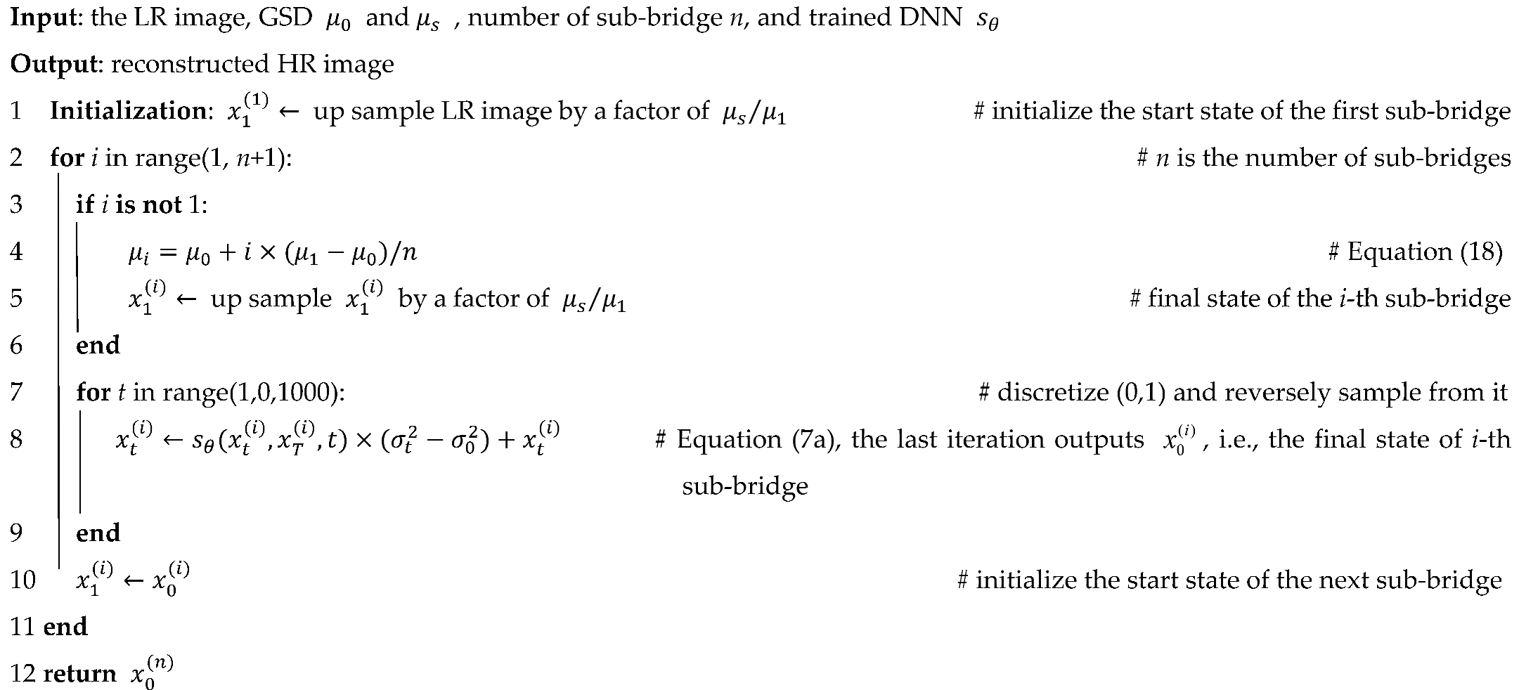 |
Algorithm 2 is essentially the backward PDSB, and it is divided into n sub-bridges. corresponding to the upsampled ST-2A image is the final state of the last PDSB, and the algorithm aims to reconstruct its paired HR image (denoted by ) in an iterative process (step 2–11). The outer iterations indexed by i iterate over all sub-bridges, and the inner iterations indexed by t reconstruct the “mile stone” in the i-th sub-bridge (i.e., ). In the reconstruction process (i.e., backward diffusion), , in line 8, is the condition of the i-th sub-bridge, and the final state (i.e., ) can be gradually reconstructed from lines 7–9. Therefore, by the coupled outer and inner iterations, the final state of the whole PDSB (i.e., ) can be progressively computed from line 2 to 11, and the HR image can be simultaneously reconstructed too. In every sampling process of sub-bridges (i.e., lines 7–9), 1000 iterations are applied.
4.2.3. DNN Architecture
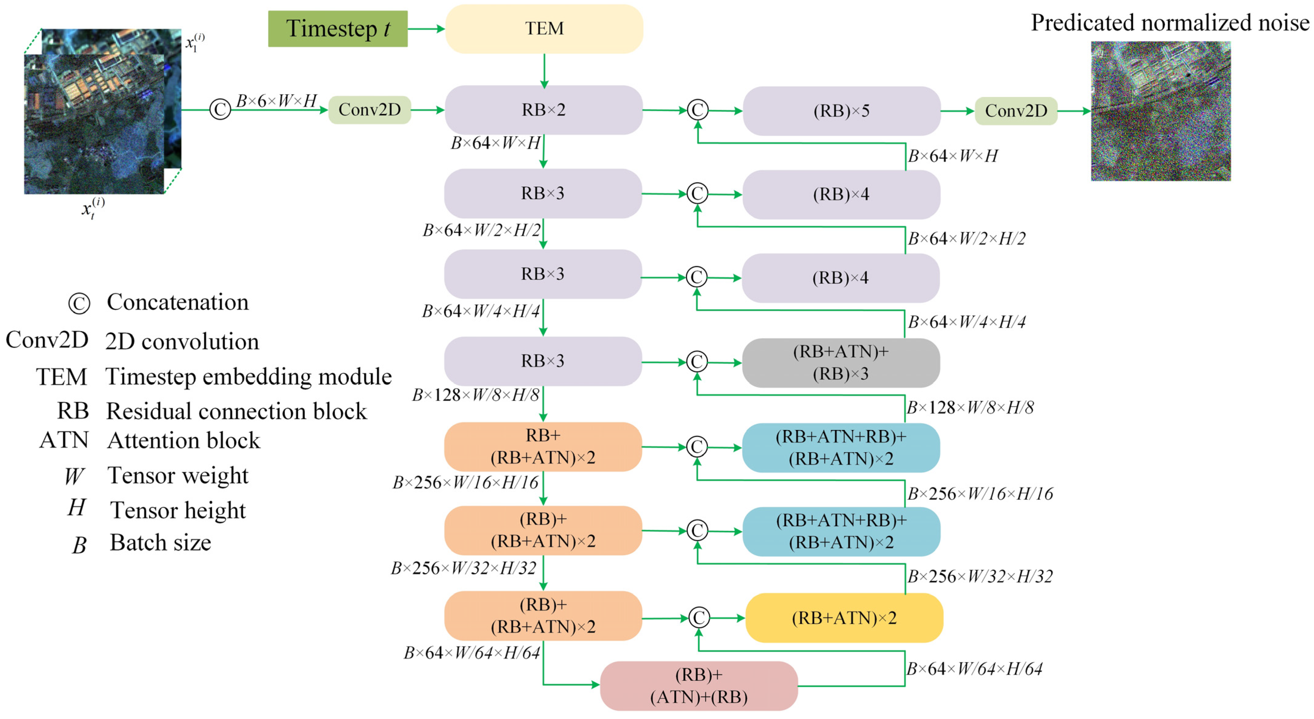
The DNN that is represented as aims to learn the logarithm gradient of given the state , and timestep t. As depicted in Equations (7a) and (16), the DNN essentially learns the negative noise (i.e., ) which is normalized by changes in the variance (i.e., ). Since and are scalars, and and have the same dimensions as the HR image, the DNN should keep the output dimensions unchanged with the input dimensions. Therefore, the U-Net is adopted to learn the normalized noise since it has both the abilities of segmenting noise and keeping dimensions unchanged. In addition, timestep t should be used as an intensity prompt of the noise level. To encode timestep t, the sinusoidal timestep embedding module is applied. The detailed architecture of the U-Net is depicted in Figure 7.
4.3. Metrics
Apart from qualitatively visual interpretation, seven quantitative metrics are applied to evaluate the effectiveness and robustness of the proposed PDSB, these metrics are FID, PSNR, SSIM, deep image structure and texture similarity (DISTS) [71], learned perceptual image patch similarity (LPIPS) [72], inception score (IS) [73], natural image quality evaluator (NIQE) [74], and average gradient (AG) [75].
FID calculated the distance of two feature sets (or distributions) that are extracted from two distinct image sets. These features are very different when they originate from different image types since they are generally output by a classifier network (e.g., Inception V3 [76]). Therefore, it aligns with human cognition that lower FID means higher similarity of two image sets, and becomes a golden standard for evaluating performances of generative models [33,34]. FID is a statistical result that cannot evaluate the similarities of individuals; PSNR compensates for the shortage since it essentially represents the mean squared error of HR and SR images. PSNR encounters evaluation problems when two images only have luminance, contrast, and structure differences; thus, SSIM (also with its lean version, DISTS) is applied to compensate for the limitation since it can maintain invariance if paired images only have the above-mentioned differences. Features used to compute FID are the final outputs of a classification network, while features irrelevant to classification are also important for human perception; thus, LPIPS is used to capture these features since it averages all features that are output by all the network layers.
Figure 7.
A detailed U-Net architecture is used to predict the normalized noise. Note that the blocks with the same basic modules are rendered with the same colors.
The above-listed five criteria are evaluated with references (i.e., the HR images), while three additional criteria (i.e., IS, NIQE, and AG) are included to specifically evaluate the quality of the SR images. Concretely, IS evaluates the distinctiveness (in the sense of classification) and diversity; NIQE represents the similarity between SR images and neural collected images; AG shows the sharpness of SR images by identifying the horizontal and vertical boundaries. The characteristics and source codes of these eight metrics are summarized in Table 1. In addition, three main metrics relevant to memory and time cost in the inference, including the number of model parameters (Para.), floating point operations (FLOPs), and inference time per frame (ITPF), are also reported.
Table 1.
Characteristics and sources of used metrics.
4.4. Comparisons with SOTAs
Eight SOTAs are chosen as the compressions, and they are efficient diffusion super-resolution (EDiffSR) [38], I2SB [53], super-resolution via repeated refinement (SR3) [36], super-resolution GAN (SRGAN) [39], very deep VAE super-resolution (VDVAESR) [27], visual autoregressive super-resolution (VARSR) [34], SRCNN [11], and Top-k Token Selective Transformer (TTST) [13]. The first three are diffusion-based SR methods, the fourth is GAN-based, the fifth is VAE-based, the sixth is VAR-based, the seventh is CNN-based, and the last is transformer-based; bicubic interpolation (BI) is used in the comparison as a baseline. All the compared SOTAs are representative and have attracted a lot of attention. In addition, to make fair competition, the eight learned methods are elaborately tuned with GFSTSR, and the learning details are listed in Table 2. All the hyperparameters are maintained, unchanged, with the source codes. To make these learned methods compatible with GPU devices, only batch sizes and LRt are tuned. Note that, for VDVAESR, since the original source code does not supply an SR of 512 × 512 pixel images, its network architecture is modified to be compatible with the image size.
Table 2.
Learning details of the six SOTAs.
4.4.1. Quantitative Comparisons
After PDSB and the SOTAs are tuned by GFSTSR of Anhui, all methods are quantitatively evaluated by GFSTSR of Hunan. The results are shown in Table 3. Note that the result of IS actually has two parts, mean and standard deviation, since the latter is much smaller compared to the former; thus, in Table 3, only the mean of it is retained.
Table 3.
Quantitative comparison results of SOTAs and PDSB.
From the quantitative results listed in Table 3, it can be seen clearly that the proposed PDSB has an overall better performance among the compared criteria. Especially for FID, PDSB is only 8.294, which is only about half of the secondary method (i.e., I2SB), and compared to the baseline method (i.e., BI), the FID of PDSB is lower than one-fifth of BI. The better FID of PDSB is mainly attributed to the merits of the diffusion model. Essentially, all the diffusion process can be unified by the forward SDE (i.e., Equation (1)), and once U-Net is trained in the forward process to make it learn the score at time t, then given the source (i.e., the LR images) distribution, it can achieve the reference (i.e., HR images) distribution by backward SDE (i.e., Equation (2)). That is, diffusion-based SR methods inherently have the merit of maintaining high consistency of HR images and the generated SR images, and this is the reason why diffusion-based methods win the majority of the top three places among all the compared methods.
Despite the merits of diffusion-based methods, PDSB has an overwhelming advantage in FID, and the success can be summarized into three aspects. Firstly, the progressive learning mode treats the upstream-generated SR images as priors; that is, the SR images are generated gradually rather than instantly. Referring to the conclusion drawn by VAR, if high-quality priors are provided, the reconstructed results will be better, thus a better FID of PDSB is almost certain. As the strong data priors are learned in the forward process of PDSB, during inference, the low-resolution images act as constraints on the solution space. With the strong learned priors, the reconstructed SR images contain plausible fine-scale features that are statistically consistent with the HR images. The high-quality priors can be evidenced by Figure 8, where the generated SR images at all scales and the corresponding ground truth HR images are presented. It can be seen clearly that the reconstructed SR images at small scales are very similar to the ground truth HR images in the appearances. For example, Figure 8c,j are the generated SR images at scale , and they are very similar to their corresponding ground truth HR images, which are respectively shown in Figure 8d,k. Therefore, with these high-quality priors (i.e., Figure 8c,j), the generated SR image at the final scale are also satisfactory.
Figure 8.
Two example scale reconstructions processed by PDSB of two sub-bridges. (a,h) are the original LR images; (b,i) are the upsampled LR images; (c,j) are the reconstructed SR images at scale ; (d,k) are the HR images at scale , i.e., the milestones in the first bridges; (e,l) are the upsampled SR images; (f,m) are the generated SR images at scale ; and (g,n) are the ground truth HR images at scale .
Secondly, PDSB decouples the SR task into sub-bridges, and every sub-bridge accomplishes an SR task with a small-scale change. As exemplified in Figure 4 and Figure 8, the original LR images are at , the first sub-bridge fulfills a sub-task that generates SR images at scale , and the task of the second sub-bridge is to SR the priors (i.e., to generate SR images at scale ) to the scale of . These two task is prone to be successful, and PDSB can outperform I2SB since scale changes are not so much.
Thirdly, geometrical displacement errors are alleviated by virtue of the existence of milestones. As exemplified in Figure 8, the original LR images (i.e., Figure 8a,h) have a GSD of 10 m, and the first milestones (i.e., Figure 8d,k) have a GSD of 6 m. If the displacement error is , then the error of the LR images and the first milestones is ; i.e., the error of the first milestones and the HR images is also half of the original. Therefore, SDEs can precisely express the evolution of images from LR to HR in PDSB, and they can generate SR images that are much more similar to the reference HR images. Since FID is the overall similarity, a better FID means other similarity metrics will not be too bad either. PDSB has the best FID; thus, other similarity metrics, such as DISTS and LPIPS, are also in the lead.
Apart from FID, PDSB also performs exceptionally well in DISTS and LPIPS. The conclusion is also supported by I2SB, as it wins second place regarding FID and, meanwhile, achieves better performances of other similarity metrics. It is interesting that the GAN-based method SRGAN has the best SSIM, though its FID is not the greatest. This is mainly because SRGAN integrates a VGG16 network to suppress perceptual losses, which enforces the textural and pixel similarity of HR and generated SR images. Apart from the first five similarity metrics, PDSB also achieves competitive results in SSIM, PSNR, NIQE, and AG.
The non-diffusion-based method TTST is also noticeable among the compared methods; it wins first place in two domains (i.e., PSNR and IS), and its FID ranks third place. The best PSNR is derived from the selective strategy of TTST, in which the most crucial tokens are retained, and the less relevant features are discarded. Since the features with higher scores (i.e., self-similarity of features) are retained, and independent noise features are discarded. Therefore, the reconstructed SR images have a higher overall similarity compared to the HR images. Whereas image details have similar characteristics to image noise, they are also sometimes discarded with noise by the selective strategy in the reconstruction process. Thus, the reconstructed images are often too smooth and lack details (this can be evidenced by Figure 9).
Figure 9.
Demonstrations of SR results of different image types. (a) Forest, (b) rivers and lakes, (c) farmlands, (d) buildings, and (e) traffic lines. For each subplot, the first row demonstrates the HR image and 2.5 times enlarged SR details, and the second and third rows are the reconstructed results of different methods. Note that, for better visualization, the LR images are upsampled to the same size as the HR images using BI, meaning they are identical to the SR results produced by BI. Zooming in on the images can provide a better view.
The selective strategy is also beneficial for the IS since noises are suppressed and the reconstructed images conform to human perception. While VARSR improves IS in a different way, it applies prefix tokens to encode information of LR images, and by using a manner of next-scale prediction, it can enhance the conspicuous textures of images (as shown in Figure 9, the conspicuous features such as roads and boundaries are well recovered); these features play an important role in classification. Meanwhile, IS evaluates distinctiveness and diversity by means of classification; thus, the characteristics of VARSAR enable it to achieve the second-best IS.
In addition, EDiffSR has the best performance in NIQE. EDiffSR is also an SDE-based method like PDSB, while it considers the diffusions as an adding noise process and utilizes a denoising network to remove as much noise as possible. It is known that noise is the key contribution to NIQE; since EDiffSR removes most of the noise, it naturally achieves the best NIQE.
The best AG is obtained by I2SB, which has a similar diffusion core to that of PDSB. I2SB can be seen as a single bridge DSB; therefore, it cannot deal with geometrical distortions and ultimately generate “speckle” textures (these textures can be found if Figure 9 is carefully examined by zooming in). These textures act like speckle noise and can give rise to higher AG, and this situation of higher AG cannot be viewed as high image quality. Among all the compared methods except for BI, VDVAESR has the worst performance in all of the metrics; this is mainly because training very deep neural networks is very tricky. Many training samples produce a gradient exploring problem and cannot be used to update the network parameters, and this problem eventually decreases the generality of VDVAESR, resulting in poor performance.
The efficiency-related parameters are presented in Table 4, and it can be seen that the computational efficiency of PDSB is naturally lower than that of I2SB as additional bridges are introduced, whereas its efficiency is not the lowest: the inference efficiency of PDSB is still superior to that of VDVAESR and VARSR. The main efficiency bottleneck of the proposed method is its requirement for hundreds or even thousands of sampling steps. If some speedup sampling strategies (e.g., ResShift [77] and TCDM [78]) are embedded in the framework, the efficiency could be further improved.
Table 4.
Comparisons of memory and time cost.
4.4.2. Qualitative Comparisons
Comparisons are also presented here for qualitative comparisons. Figure 9 demonstrates the generated SR results of five types (i.e., forest, rivers and lakes, farmlands, buildings, and traffic lines) of images. Though different types of images have distinctive textural patterns and an imbalanced number of training samples, it can be seen clearly that the reconstruction results of the PDSB are robust and outperform other methods.
Other methods apart from PDSB also have distinctive features of SR results. Although the overall SR results of I2SB have a very close appearance to that of PDSB, it can be seen clearly from the enlarged details that the SR results of I2SB have “speckle” textures, and the “speckles” are mainly results from geometrical displacements, which cannot be modeled by Gaussian diffusion. This conclusion is also certified by the other two diffusion-based methods (i.e., SR3 and EDiffSR), while the “speckle” effect in the SR results of SR3 and EDiffSR is much more severe and manifested as distorted and incomplete textures.
In addition, one of the noticeable phenomena among the SR images is that VARSR tends to reconstruct the distinguishing features (e.g., edges) of the image. As shown in Figure 9c,e, the roads in the images are clearly reconstructed even though they are over-sharpened. This is because VARSR uses a block-wise strategy to reconstruct image details. This strategy models the block-wise dependencies sequentially and concentrates on coherence between blocks, enabling it to reconstruct distinguishing features like edges. Additionally, VARSR incorporates a local attention [9] mechanism which focuses on reconstructing high-frequency details (e.g., edges). The attention mechanism is also used by TTST; the SR results of TTST resemble those of VARSR: edges are over-sharpened, and low-frequency signals (e.g., mild textural changes in the farmlands) are smoothed.
The SR images of SRGAN and SRCNN are visually similar. As presented in Table 3, quantized metrics of the two methods, apart from AG, are also very close. The main reason is that the two methods are both CNN-based (specifically, SRGAN is VGG-style, and SRCNN just consists of three convolutional layers) and have essentially the same optimization objective: SRCNN minimizes the mean-squared-error (MSE) loss; for SRGAN, MSE contributes the primary loss, although adversarial loss is included.
4.5. Ablation Experiments
To examine the sensitivity of the proposed method to different hyperparameters, two ablation experiments are conducted. Two main hyperparameters, n (i.e., number of sub-bridges) and (i.e., the tolerance of geometrical displacements), are concerned with testing the stability and cost of the proposed method. Since FID is a golden metric for evaluating an SR result, it is used to represent the effect of the parametric variations.
4.5.1. Efficiency and Effectiveness Change with Variation in n
Theoretically, as analyzed in Section 3.3, a greater n will be beneficial for the performance while harmful for the productivity. To trade off efficiency and effectiveness, the SR results presented above are achieved by PDSB with two sub-bridges (i.e., n = 2); the balance is obtained by ablation experiments that are done with n = 1, 3, 4 and 5, and FID and average inferring time per image are recorded as indicators (the results are presented in Figure 10). Note that, when n = 1, PDSB is degenerated to I2SB.
Figure 10.
FID and inferring time, varying with increasing sub-bridge numbers.
It can be seen clearly from Figure 10 that FID drops sharply when n increases from 1 to 2, and it declines slightly when n increases from 2 to 5. Meanwhile, inference time is approximately proportional to n. That is to say, the SR results can be enhanced if a greater n is supplied, while this enhancement is limited when n exceeds 2. Since the scale change and geometrical displacements of a paired LR-HR image are not great, two-part bridges are sufficient to model the diffusion process, and more bridges cannot result in further increments. Inferring time is always proportional to n since every sub-bridge finishes the same SR task and costs approximately equal inferring time. For practical applications, the displacements are hardly more than 5 pixels. Therefore, n = 2 is the optimal choice.
4.5.2. Side Effects of Increasing
It has been theoretically analyzed in Section 3.1 and Section 3.2 that the Gaussian diffusion model cannot model the displacements; thus, PDSB was designed to alleviate the side effects of the displacements. To evaluate the extent of its tolerance, experiments were conducted under varying displacement conditions (note that the results were achieved by PDSB with two sub-bridges). For the practically used georeferencing and registration method of RSIs, the displacement rarely exceeds 10 pixels [79]; thus, in the experiments, the maximum value of τ is set to 10 pixels. The displacement τ is divided into three levels: 0–5 pixels, 5–8 pixels and 8–10 pixels. The error in the original GFSTSR dataset is 0–5 pixels, and the last two levels of learning data are produced by adding a certain random displacement to the original GFSTSR dataset. These three datasets are used to train three PDSB models, and then they are used to reconstruct SR images; FIDs are, respectively, calculated and demonstrated in Table 5, and reconstructed SR image examples are presented in Figure 11.
Table 5.
FIDs vary with the different displacement levels.
Figure 11.
HR images and the reconstructed SR images. (a) HR images, and (b), (c), and (d) are the reconstructed SR images with respective average displacement levels of 5, 8, and 10 pixels, respectively.
For the first displacement level (i.e., displacement of 0–5 pixels), it is identical to that of the GFSTSR dataset; thus, the FID of SR images is also the same as presented in Table 3 of PDSB. And when the displacement level ranges from 5 to 8 pixels, the FID is 14.841, which is close to the FID of I2SB when it is trained in original GFSTSR dataset (16.883 as shown in Table 3), and by examining Figure 11c, it can be found that the generated SR image also have “speckles” which is the textural characteristic of I2SB. As the displacement level increases to 8–10 pixels, FID also increases to 30.524, and from Figure 11d it can be seen that “speckles” become pure noise and texture details are not recovered. Thus, for training PDSB, the optimal displacement is less than 5 pixels, while displacements greater than 8 pixels lead to poor performance of the trained PDSB. To enhance the robustness of PDSB against varying displacement levels, one straightforward approach is to introduce additional sub-bridges. Alternatively, a deep neural network (DNN) could be employed to predict the displacement between LR and HR images. The predicted displacement can then be used to re-register the image pair, enabling the newly aligned pair to improve PDSB’s robustness to displacement during training.
It is worth noting that the side effects of displacement on other SR methods are much more severe. For example, if SRCNN is trained on the dataset with and without displacement, the SR results will make a big difference. Figure 12 illustrates the results.
Figure 12.
Example SR images by SRCNN trained with a different dataset. The upper and lower rows are corresponding SR images of SRCNN, which is trained on the dataset without displacement and with 10-pixel displacements, respectively.
To accurately simulate the displacements, both the LR and HR images are derived from GF6 images. The HR images are cropped from GF6 images with a size of 512 × 512 pixels. To create LR images without displacements, the original cropped HR images are first downsampled to 103 × 103 pixels and then upsampled to 512 × 512 pixels. As a comparison, to accurately simulate a dataset with displacements, the HR images are also cropped from GF6 with a size of 512 × 512 pixels. To add displacements, the HR images are firstly added to 0–20 uniformly distributed pixels (corresponding to 0–40 meters’ geographic position errors). Then, displacement-contaminated images are first resized to 103 × 103 pixels and then upsampled to 512 × 512 pixels. Therefore, in the dataset with displacement, LR images and HR images have a scale difference of five times, and the average displacement is 10 pixels. As illustrated in Figure 12, SR images of SRCNN trained without displacement distinctly outperform those trained on a dataset with 10-pixel displacement. Qualitative results presented in Table 6 are also consistent with the visual results illustrated in Figure 12.
Table 6.
Qualitative comparison of the results of SRCNN, which is trained with and without displacements.
5. Conclusions and Future Works
The paper proposed a progressive diffusion model named PDSB, aiming to cope with the geometrical displacements that are commonly presented in learning datasets of SR tasks. PDSB decouples an SR task into sub-bridges, and each sub-bridge accomplishes an SR task with a small-scale change. The upstream reconstructed SR images are viewed as priors; therefore, geometrical displacement errors are alleviated by virtue of the existence of priors. The proposed PDSB is compared with SOTA methods such as EDiffSR, I2SB, SR3, SRGAN, VARSR, and VDVAESR, and experimental results show that it outperforms the SOTAs in FID, PSNR, DISTS, and LPIPS. Specifically, for FID, it is only half of I2SB, which wins second place in the comparison. Ablation experiments reveal that if the displacement errors existing in the training data are lower than 5 pixels, PDSB with two sub-bridges can be immune to this level of displacement errors and can be trained for practical use. In short, if the displacement is greater than five pixels, the sub-bridges are necessary; to balance efficiency and effectiveness for the practical use of SRI SR, it is appropriate to set the sub-bridge to two. Moreover, regardless of the magnitude of the displacement, dividing DSB into sub-bridges is always beneficial, since it alleviates the displacement problem.
Although the results achieved by PDSB are satisfactory, the effect that divide DSB into sub-bridges to alleviate displacements is limited. Theoretically, if greater displacements are presented, a greater number of sub-bridges should be applied, whereas a greater number of sub-bridges means more computational expenditures, which will result in an unwieldy SR method if the number of sub-bridges exceeds a certain extent. Future works will design a displacement awareness network (e.g., an optical flow network or spatial transformer network) to learn displacements. Another option is to provide a closed-form expression of displacement propagation across sub-bridges. Furthermore, this work is concentrated on the probabilistic learning scheme; the network architecture (i.e., U-Net) is used as the original without any improvement. Future work will also consider the textural characteristics of RSI and design a modified version of U-Net to recover more details in SR images.
Author Contributions
Conceptualization, S.C. and C.D.; methodology, S.C. and Y.Z.; validation, Y.Z.; formal analysis, Y.Z.; data curation, T.Z.; writing—original draft preparation, S.C., Z.L. and H.L.; writing—review and editing, S.C. and C.D.; visualization, T.Z.; supervision, S.C. and C.D.; project administration, C.D.; funding acquisition, S.C. All authors have read and agreed to the published version of the manuscript.
Funding
This work was supported in part by the National Natural Science Foundation of China, under Grant 41901402; in part by the Open Fund of Key Laboratory of Investigation, Monitoring, Protection and Utilization for Cultivated Land Resources, Ministry of Natural Resources, under Grant CLRKL2024KP04; in part by the Nanhu Scholars Program for Young Scholars of XYNU, under Grant 2017037; and in part by the Key Scientific and Technological Research Project of Henan Province, under Grant 252102110354; and in part by the Scientific Research Fund of Wuzhou University, under Grant WZUQDJJ43022.
Data Availability Statement
The data and codes are available on https://github.com/csyhy1986/PDSB (accessed on 1 February 2026).
Conflicts of Interest
The authors declare no conflicts of interest.
References
- Baker, S.; Kanade, T. Limits on super-resolution and how to break them. IEEE Trans. Pattern Anal. Mach. Intell. 2002, 24, 1167–1183. [Google Scholar] [CrossRef] [Scilit]
- Wang, Z.; Chen, J.; Hoi, S.C.H. Deep learning for image super-resolution: A survey. IEEE Trans. Pattern Anal. Mach. Intell. 2020, 43, 3365–3387. [Google Scholar] [CrossRef] [Scilit] [PubMed]
- Salari, A.; Djavadifar, A.; Liu, X.; Najjaran, H. Object recognition datasets and challenges: A review. Neurocomputing 2022, 495, 129–152. [Google Scholar] [CrossRef] [Scilit]
- Shafique, A.; Cao, G.; Khan, Z.; Asad, M.; Aslam, M. Deep Learning-Based Change Detection in Remote Sensing Images: A Review. Remote Sens. 2022, 14, 871. [Google Scholar] [CrossRef] [Scilit]
- Meer, F.V.D. Remote-sensing image analysis and geostatistics. Int. J. Remote Sens. 2012, 33, 5644–5676. [Google Scholar] [CrossRef] [Scilit]
- Liu, Y.; Wang, S.; Zhang, J.; Wang, S.; Ma, S.; Gao, W. Iterative network for image super-resolution. IEEE Trans. Multimed. 2021, 24, 2259–2272. [Google Scholar] [CrossRef] [Scilit]
- Yang, J.; Wang, Z.; Lin, Z.; Cohen, S.; Huang, T. Coupled dictionary training for image super-resolution. IEEE Trans. Image Process. 2012, 21, 3467–3478. [Google Scholar] [CrossRef] [Scilit]
- Lecun, Y.; Boser, B.; Denker, J.; Henderson, D.; Howard, R.; Hubbard, W.; Jackel, L.D. Backpropagation applied to handwritten zip code recognition. Neural Comput. 1989, 1, 541–551. [Google Scholar] [CrossRef] [Scilit]
- Vaswani, A.; Shazeer, N.; Parmar, N.; Uszkoreit, J.; Jones, L.; Gomez, A.N.; Kaiser, L.; Polosukhin, I. Attention is all you need. arXiv 2017, arXiv:1706.03762. [Google Scholar]
- Gu, A.; Dao, T. Mamba: Linear-time sequence modeling with selective state spaces. arXiv 2023, arXiv:2312.00752. [Google Scholar] [CrossRef] [Scilit]
- Dong, C.; Loy, C.C.; He, K.; Tang, X. Image super-resolution using deep convolutional networks. IEEE Trans. Pattern Anal. Mach. Intell. 2015, 38, 295–307. [Google Scholar] [CrossRef] [Scilit]
- Xiao, Y.; Yuan, Q.; Jiang, K.; Chen, Y.; Wang, S.; Lin, C.W. Multi-Axis Feature Diversity Enhancement for Remote Sensing Video Super-Resolution. IEEE Trans. Image Process. 2025, 34, 1766–1778. [Google Scholar] [CrossRef] [Scilit]
- Xiao, Y.; Yuan, Q.; Jiang, K.; He, J.; Lin, C.; Zhang, L. TTST: A top-k token selective transformer for remote sensing image super-resolution. IEEE Trans. Image Process. 2024, 33, 738–752. [Google Scholar] [CrossRef] [Scilit]
- Li, X.; Xu, F.; Liu, F.; Lyu, X.; Tong, Y.; Xu, Z.; Zhou, J. A synergistical attention model for semantic segmentation of remote sensing images. IEEE Trans. Geosci. Remote Sens. 2023, 61, 5400916. [Google Scholar] [CrossRef] [Scilit]
- Li, X.; Xu, F.; Liu, F.; Tong, Y.; Lyu, X.; Zhou, J. Semantic segmentation of remote sensing images by interactive representation refinement and geometric prior-guided inference. IEEE Trans. Geosci. Remote Sens. 2023, 62, 5400318. [Google Scholar] [CrossRef] [Scilit]
- Li, X.; Xu, F.; Yu, A.; Lyu, X.; Gao, H.; Zhou, J. A Frequency Decoupling Network for Semantic Segmentation of Remote Sensing Images. IEEE Trans. Geosci. Remote Sens. 2025, 63, 5607921. [Google Scholar] [CrossRef] [Scilit]
- Li, X.; Xu, F.; Zhang, J.; Yu, A.; Lyu, X.; Gao, H.; Zhou, J. Dual-domain decoupled fusion network for semantic segmentation of remote sensing images. Inf. Fusion 2025, 124, 103359. [Google Scholar] [CrossRef] [Scilit]
- Xiao, Y.; Yuan, Q.; Jiang, K.; Chen, Y.; Zhang, Q.; Lin, C.W. Frequency-assisted mamba for remote sensing image super-resolution. IEEE Trans. Multimed. 2024, 27, 1783–1796. [Google Scholar] [CrossRef] [Scilit]
- Zhi, R.; Fan, X.; Shi, J. MambaFormerSR: A Lightweight Model for Remote-Sensing Image Super-Resolution. IEEE Geosci. Remote Sens. Lett. 2024, 21, 6015705. [Google Scholar] [CrossRef] [Scilit]
- Zhao, G.; Wang, F. Mamba-Based Residual Network for Remote Sensing Image Super-Resolution. In Proceedings of the International Conference on Pattern Recognition and Artificial Intelligence (ICPRAI), Jeju Island, Republic of Korea, 18–21 June 2024; pp. 316–321. [Google Scholar]
- Murphy, K.P. Machine Learning: A Probabilistic Perspective; MIT Press: Cambridge, MA, USA, 2012; pp. 65–98. [Google Scholar]
- Bishop, C.M.; Nasrabadi, N.M. Pattern Recognition and Machine Learning; Springer: New York, NY, USA, 2006; pp. 196–202. [Google Scholar]
- Cao, H.; Tan, C.; Gao, Z.; Xu, Y.; Chen, G.; Heng, P.A.; Li, S. A survey on generative diffusion models. IEEE Trans. Knowl. Data Eng. 2024, 36, 2814–2830. [Google Scholar] [CrossRef] [Scilit]
- Yang, L.; Zhang, Z.; Song, Y.; Hong, S.; Xu, R.; Zhao, Y.; Zhang, W.; Cui, B.; Yang, M. Diffusion models: A comprehensive survey of methods and applications. ACM Comput. Surv. 2023, 56, 105. [Google Scholar] [CrossRef] [Scilit]
- Diederik, P.K.; Max, W. Auto-encoding variational Bayes. In Proceedings of the International Conference on Learning Representations (ICLR), Banff, AB, Canada, 14–16 April 2014; pp. 1–14. [Google Scholar]
- Kim, J.; Kong, J.; Son, J. Conditional variational autoencoder with adversarial learning for end-to-end text-to-speech. In Proceedings of the International Conference on Machine Learning (ICML), Virtual Event, 18–24 July 2021; pp. 5530–5540. [Google Scholar]
- Chira, D.; Haralampiev, I.; Winther, O.; Dittadi, A.; Liévin, V. Image super-resolution with deep variational autoencoders. In Proceedings of the European Conference on Computer Vision (ECCV), Tel Aviv, Israel, 25–27 October 2022; pp. 395–411. [Google Scholar]
- Goodfellow, I.; Pouget-Abadie, J.; Mirza, M.; Xu, B.; Warde-Farley, D.; Ozair, S.; Courville, A.; Bengio, Y. Generative adversarial networks. Commun. ACM 2020, 63, 139–144. [Google Scholar] [CrossRef] [Scilit]
- Ledig, C.; Theis, L.; Huszár, F.; Caballero, J.; Cunningham, A.; Acosta, A.; Aitken, A.; Tejani, A.; Totz, J.; Wang, Z.; et al. Photo-realistic single image super-resolution using a generative adversarial network. In Proceedings of the IEEE Conference on Computer Vision and Pattern Recognition (CVPR), Honolulu, HI, USA, 21–26 July 2017; pp. 105–114. [Google Scholar]
- Wang, X.; Yu, K.; Wu, S.; Gu, J.; Liu, Y.; Dong, C.; Qiao, Y.; Loy, C.C. Esrgan: Enhanced super-resolution generative adversarial networks. In Proceedings of the European Conference on Computer Vision (ECCV), Munich, Germany, 8–14 September 2018; pp. 63–79. [Google Scholar]
- Papamakarios, G.; Nalisnick, E.; Rezende, D.J.; Mohamed, S.; Lakshminarayanan, B. Normalizing flows for probabilistic modeling and inference. J. Mach. Learn. Res. 2021, 22, 1–64. [Google Scholar]
- Lugmayr, A.; Danelljan, M.; Van Gool, L.; Timofte, R. SRFlow: Learning the super-resolution space with normalizing flow. In Proceedings of the European Conference on Computer Vision (ECCV), Glasgow, UK, 23–28 August 2020; pp. 715–732. [Google Scholar]
- Tian, K.; Jiang, Y.; Yuan, Z.; Peng, B.; Wang, L. Visual autoregressive modeling: Scalable image generation via next-scale prediction. In Proceedings of the Advances in Neural Information Processing Systems 37 (NeurIPS 2024), Vancouver, BC, Canada, 10–15 December 2024; pp. 84839–84865. [Google Scholar]
- Qu, Y.; Yuan, K.; Hao, J.; Zhao, K.; Xie, Q.; Sun, M.; Zhou, C. Visual Autoregressive Modeling for Image Super-Resolution. arXiv 2025, arXiv:2501.18993. [Google Scholar] [CrossRef] [Scilit]
- Moser, B.; Shanbhag, A.; Raue, F.; Frolov, S.; Palacio, S.; Dengel, A. Diffusion models, image super-resolution, and everything: A survey. IEEE Trans. Neural Netw. Learn. Syst. 2024, 36, 11793–11813. [Google Scholar] [CrossRef] [Scilit]
- Saharia, C.; Ho, J.; Chan, W.; Salimans, T.; Fleet, D.J.; Norouzi, M. Image super-resolution via iterative refinement. IEEE Trans. Pattern Anal. Mach. Intell. 2022, 45, 4713–4726. [Google Scholar] [CrossRef] [Scilit]
- Xiao, Y.; Yuan, Q.; Jiang, K.; He, J.; Jin, X.; Zhang, L. EDiffSR: An efficient diffusion probabilistic model for remote sensing image super-resolution. IEEE Trans. Geosci. Remote Sens. 2023, 62, 5601514. [Google Scholar] [CrossRef] [Scilit]
- Lin, X.; He, J.; Chen, Z.; Lyu, Z.; Dai, B.; Yu, F.; Qiao, Y.; Ouyang, W.; Dong, C. Diffbir: Toward blind image restoration with generative diffusion prior. In Proceedings of the European Conference on Computer Vision (ECCV), Milan, Italy, 29 September–4 October 2024; pp. 430–448. [Google Scholar]
- Wang, C.; Sun, W. Semantic guided large scale factor remote sensing image super-resolution with generative diffusion prior. ISPRS J. Photogramm. Remote Sens. 2025, 220, 125–138. [Google Scholar] [CrossRef] [Scilit]
- Maeda, S. Unpaired image super-resolution using pseudo-supervision. In Proceedings of the IEEE Conference on Computer Vision and Pattern Recognition (CVPR), Seattle, WA, USA, 13–19 June 2020; pp. 291–300. [Google Scholar]
- Prajapati, K.; Chudasama, V.; Patel, H.; Upla, K.; Raja, K.; Ramachandra, R.; Busch, C. Direct unsupervised super-resolution using generative adversarial network (DUS-GAN) for real-world data. IEEE Trans. Image Process. 2021, 30, 8251–8264. [Google Scholar] [CrossRef] [Scilit] [PubMed]
- Wang, K.; Gou, C.; Duan, Y.; Lin, Y.; Zheng, X.; Wang, F. Generative adversarial networks: Introduction and outlook. IEEE-CAA J. Autom. Sin. 2017, 4, 588–598. [Google Scholar] [CrossRef] [Scilit]
- Lipman, Y.; Chen, R.; Ben-Hamu, H.; Nickel, M.; Le, M. Flow matching for generative modeling. arXiv 2022, arXiv:2210.02747. [Google Scholar]
- Martin, S.; Gagneux, A.; Hagemann, P.; Steidl, G. PnP-Flow: Plug-and-play image restoration with flow matching. arXiv 2024, arXiv:2410.02423. [Google Scholar]
- Kirichenko, P.; Izmailov, P.; Wilson, A.G. Why normalizing flows fail to detect out-of-distribution data. In Proceedings of the Advances in Neural Information Processing Systems 33 (NeurIPS 2020), Vancouver, BC, Canada, 6–12 December 2020; pp. 20578–20589. [Google Scholar]
- Ke, Y.; Li, X.; Liang, Y.; Shi, Z.; Song, Z. Circuit complexity bounds for visual autoregressive model. arXiv 2025, arXiv:2501.04299. [Google Scholar] [CrossRef] [Scilit]
- Zhai, S.; Zhang, R.; Nakkiran, P.; Berthelot, D.; Gu, J.; Zheng, H.; Chen, T.; Bautista, M.; Jaitly, N.; Susskind, J. Normalizing flows are capable generative models. arXiv 2024, arXiv:2412.06329. [Google Scholar] [CrossRef] [Scilit]
- Wang, Z.; Zheng, H.; He, P.; Chen, W.; Zhou, M. Diffusion-GAN: Training GANs with Diffusion. arXiv 2022, arXiv:2206.02262. [Google Scholar]
- Ho, J.; Jain, A.; Abbeel, P. Denoising diffusion probabilistic models. In Proceedings of the Advances in Neural Information Processing Systems 33 (NeurIPS 2020), Vancouver, BC, Canada, 6–12 December 2020; pp. 6840–6851. [Google Scholar]
- Song, Y.; Ermon, S. Generative modeling by estimating gradients of the data distribution. In Proceedings of the Advances in Neural Information Processing Systems 32 (NeurIPS 2019), Vancouver, BC, Canada, 8–14 December 2019; pp. 11918–11930. [Google Scholar]
- Song, Y.; Sohl-Dickstein, J.; Kingma, D.P.; Kumar, A.; Ermon, S.; Poole, B. Score-based generative modeling through stochastic differential equations. arXiv 2020, arXiv:2011.13456. [Google Scholar]
- De, B.V.; Thornton, J.; Heng, J.; Doucet, A. Diffusion schrödinger bridge with applications to score-based generative modeling. In Proceedings of the Advances in Neural Information Processing Systems 34 (NeurIPS 2021), Vancouver, BC, Canada, 6–14 December 2021; pp. 17695–17709. [Google Scholar]
- Liu, G.; Vahdat, A.; Huang, D.; Theodorou, E.A.; Nie, W.; Anandkumar, A. I2SB: Image-to-Image Schrödinger Bridge. arXiv 2023, arXiv:2302.05872. [Google Scholar]
- Su, X.; Song, J.; Meng, C.; Ermon, S. Dual diffusion implicit bridges for image-to-image translation. arXiv 2022, arXiv:2203.08382. [Google Scholar]
- Xia, T.; He, Z.; Cai, Z.; Wang, C.; Wang, W.; Wang, J.; Hu, Q.; Song, Q. Exploring the potential of Chinese GF-6 images for crop mapping in regions with complex agricultural landscapes. Int. J. Appl. Earth Obs. Geoinf. 2022, 107, 102702. [Google Scholar] [CrossRef] [Scilit]
- Observing the Earth—Sentinel-2. Available online: https://www.esa.int/Applications/Observing_the_Earth/Copernicus/Sentinel-2 (accessed on 14 August 2025).
- Heusel, M.; Ramsauer, H.; Unterthiner, T.; Nessler, B.; Hochreiter, S. Gans trained by a two time-scale update rule converge to a local Nash equilibrium. In Proceedings of the Advances in Neural Information Processing Systems 30 (NeurIPS 2017), Long Beach, CA, USA, 4–9 December 2017; pp. 6629–6640. [Google Scholar]
- Thomos, N.; Boulgouris, N.V.; Strintzis, M.G. Optimized transmission of JPEG2000 streams over wireless channels. IEEE Trans. Image Process. 2005, 15, 54–67. [Google Scholar] [CrossRef] [Scilit]
- Wang, Z.; Bovik, A.C.; Sheikh, H.R.; Simoncelli, E.P. Image quality assessment: From error visibility to structural similarity. IEEE Trans. Image Process. 2004, 13, 600–612. [Google Scholar] [CrossRef] [Scilit]
- Oksendal, B. Stochastic Differential Equations: An Introduction with Applications; Springer Science & Business Media: Heidelberg/Berlin, Germany, 2013; pp. 21–37. [Google Scholar]
- Schowengerdt, R.A. Remote Sensing: Models and Methods for Image Processing; Elsevier: Amsterdam, The Netherlands, 2006; pp. 324–355. [Google Scholar]
- Applebaum, D. Lévy Processes and Stochastic Calculus; Cambridge University Press: Cambridge, UK, 2009; pp. 243–278. [Google Scholar]
- Ronneberger, O.; Fischer, P.; Brox, T. U-net: Convolutional networks for biomedical image segmentation. In Proceedings of the Medical Image Computing and Computer-Assisted Intervention (MICCAI), Munich, Germany, 5–9 October 2015; pp. 234–241. [Google Scholar]
- Särkkä, S.; Solin, A. Applied Stochastic Differential Equations; Cambridge University Press: Cambridge, UK, 2019; pp. 42–58. [Google Scholar]
- Chen, T.; Liu, G.; Tao, M.; Theodorou, E.A. Deep momentum multi-marginal Schrödinger bridge. In Proceedings of the Advances in Neural Information Processing Systems 36 (NeurIPS 2023), New Orleans, LA, USA, 11–16 December 2023; pp. 57058–57086. [Google Scholar]
- Chen, Y.; Conforti, G.; Georgiou, T.; Ripani, L. Multi-marginal Schrödinger bridges. In Proceedings of the International Conference on Geometric Science of Information (GSI), Toulouse, France, 27–29 August 2019; pp. 725–732. [Google Scholar]
- Theodoropoulos, P.; Saravanos, A.D.; Theodorou, E.A.; Liu, G. Momentum Multi-Marginal Schrödinger Bridge Matching. arXiv 2025, arXiv:2506.10168. [Google Scholar] [CrossRef] [Scilit]
- Yi, K.M.; Trulls, E.; Ono, Y.; Lepetit, V.; Salzmann, M.; Fua, P. Learning to Find Good Correspondences. In Proceedings of the IEEE Conference on Computer Vision and Pattern Recognition (CVPR), Salt Lake City, UT, USA, 18–23 June 2018; pp. 2666–2674. [Google Scholar]
- Baarda, W. A testing procedure for use in geodetic networks. Neth. Geod. Comm. 1968, 2, 2–5. [Google Scholar] [CrossRef] [Scilit]
- Kingma, D.P.; Ba, J. Adam: A method for stochastic optimization. arXiv 2014, arXiv:1412.6980. [Google Scholar]
- Ding, K.; Ma, K.; Wang, S.; Simoncelli, E.P. Image quality assessment: Unifying structure and texture similarity. IEEE Trans. Pattern Anal. Mach. Intell. 2020, 44, 2567–2581. [Google Scholar] [CrossRef] [Scilit] [PubMed]
- Zhang, R.; Isola, P.; Efros, A.A.; Shechtman, E.; Wang, O. The unreasonable effectiveness of deep features as a perceptual metric. In Proceedings of the IEEE Conference on Computer Vision and Pattern Recognition (CVPR), Salt Lake City, UT, USA, 18–23 June 2018; pp. 586–595. [Google Scholar]
- Salimans, T.; Goodfellow, I.; Zaremba, W.; Cheung, V.; Radford, A.; Chen, X. Improved techniques for training gans. In Proceedings of the Advances in Neural Information Processing Systems 29 (NeurIPS 2016), Barcelona, Spain, 5–10 December 2016; pp. 2234–2242. [Google Scholar]
- Mittal, A.; Soundararajan, R.; Bovik, A.C. Making a “completely blind” image quality analyzer. IEEE Signal Process. Lett. 2012, 20, 209–212. [Google Scholar] [CrossRef] [Scilit]
- Shu, L.; Zhu, Q.; He, Y.; Chen, W.; Yan, J. A survey of super-resolution image quality assessment. Neurocomputing 2025, 621, 129279. [Google Scholar] [CrossRef] [Scilit]
- Szegedy, C.; Vanhoucke, V.; Ioffe, S.; Shlens, J.; Wojna, Z. Rethinking the inception architecture for computer vision. In Proceedings of the IEEE Conference on Computer Vision and Pattern Recognition (CVPR), Las Vegas, NV, USA, 27–30 June 2016; pp. 2818–2826. [Google Scholar]
- Yue, Z.; Wang, J.; Loy, C.C. Resshift: Efficient diffusion model for image super-resolution by residual shifting. Adv. Neural Inf. Process. Syst. 2023, 36, 13294–13307. [Google Scholar]
- Zhang, Y.; Liu, H.; Li, Z.; Gao, X.; Shi, G.; Jiang, J. TCDM: Effective large-factor image super-resolution via texture consistency diffusion. IEEE Trans. Geosci. Remote Sens. 2024, 62, 5609613. [Google Scholar] [CrossRef] [Scilit]
- Long, T.; Jiao, W.; He, G.; Zhang, Z. A fast and reliable matching method for automated georeferencing of remotely-sensed imagery. Remote Sens. 2016, 8, 56. [Google Scholar] [CrossRef] [Scilit]
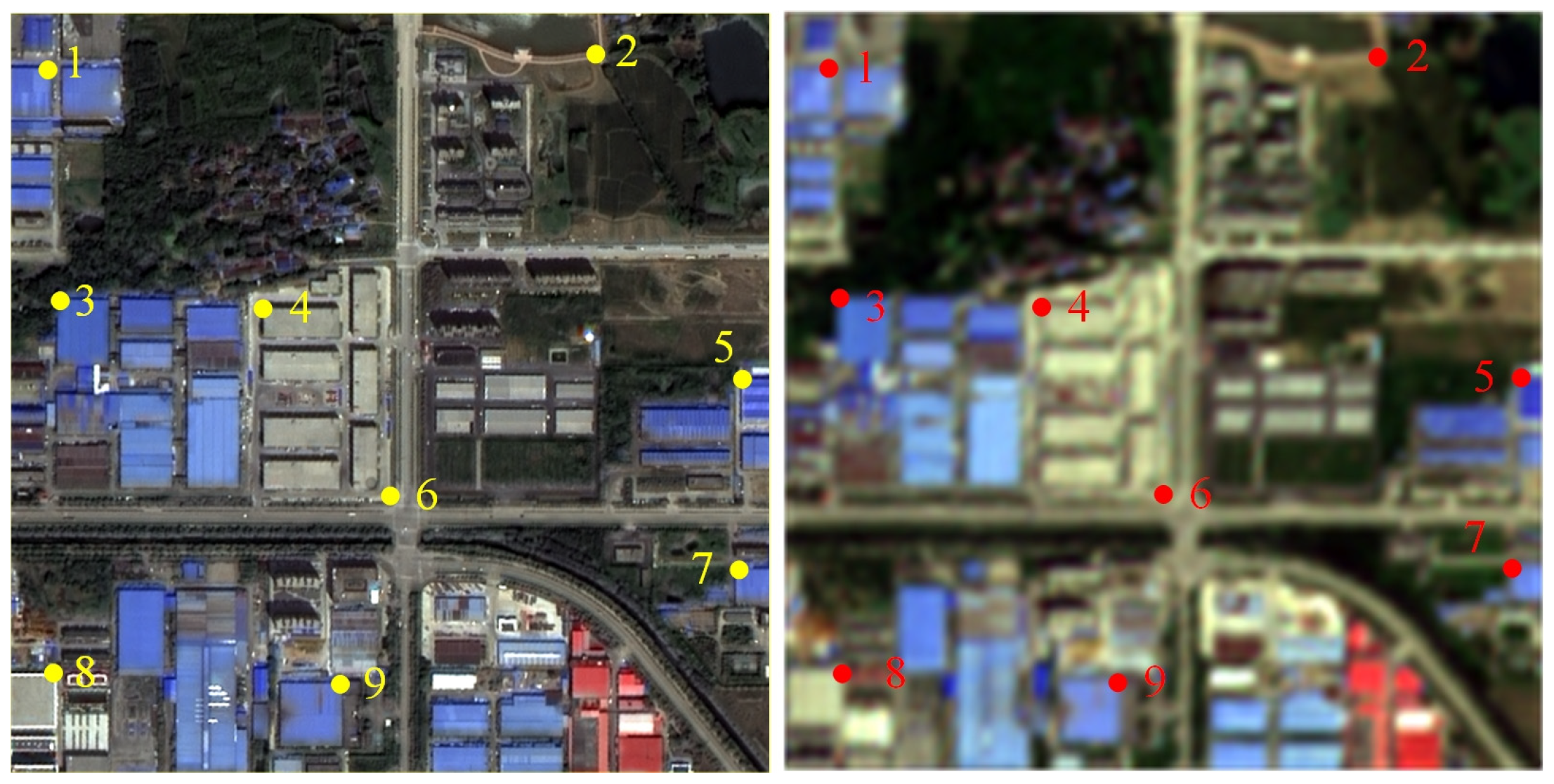
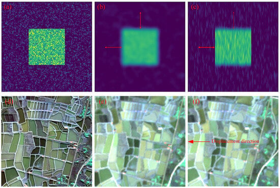
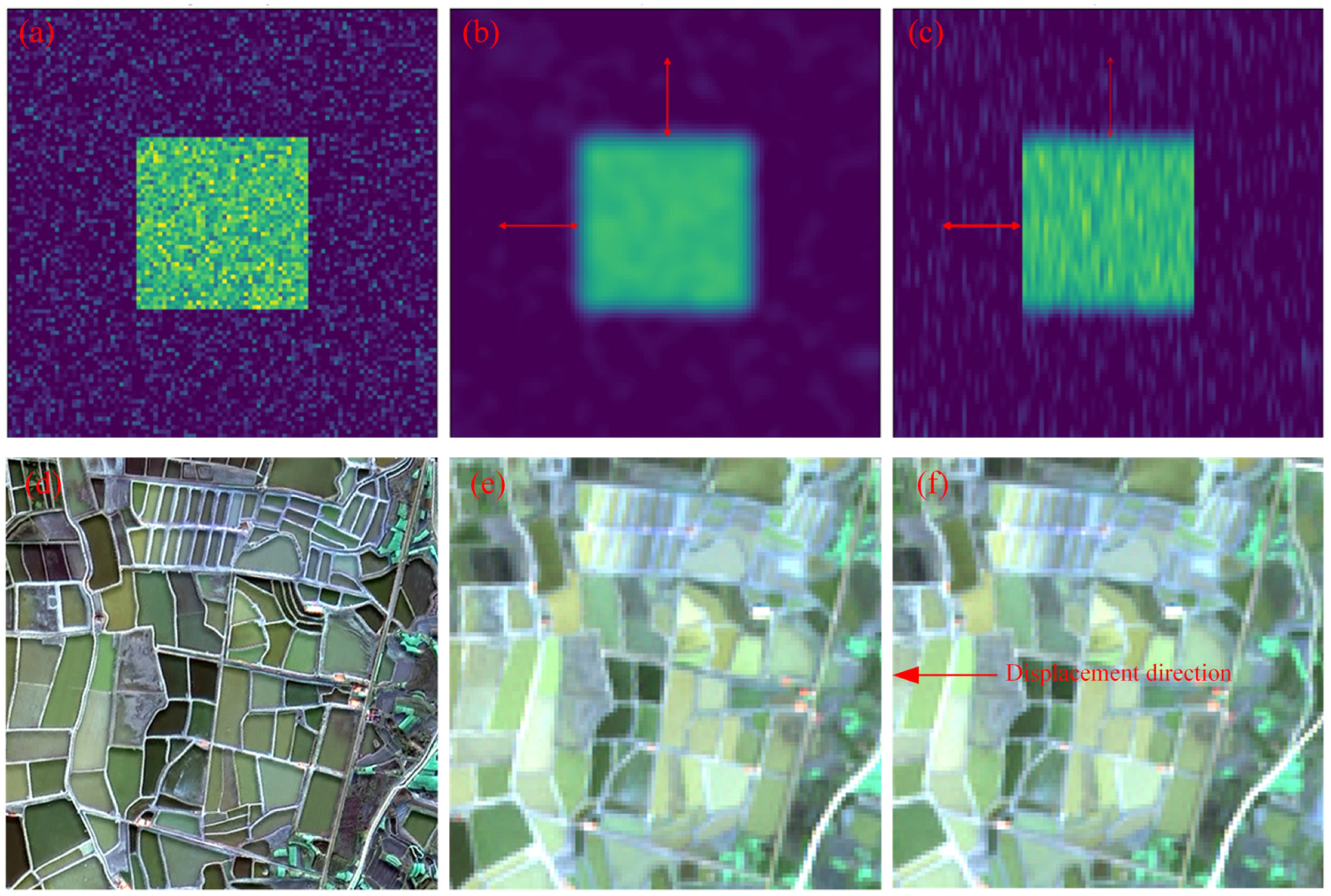
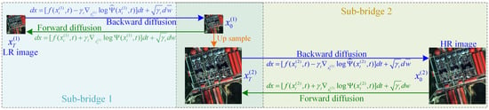
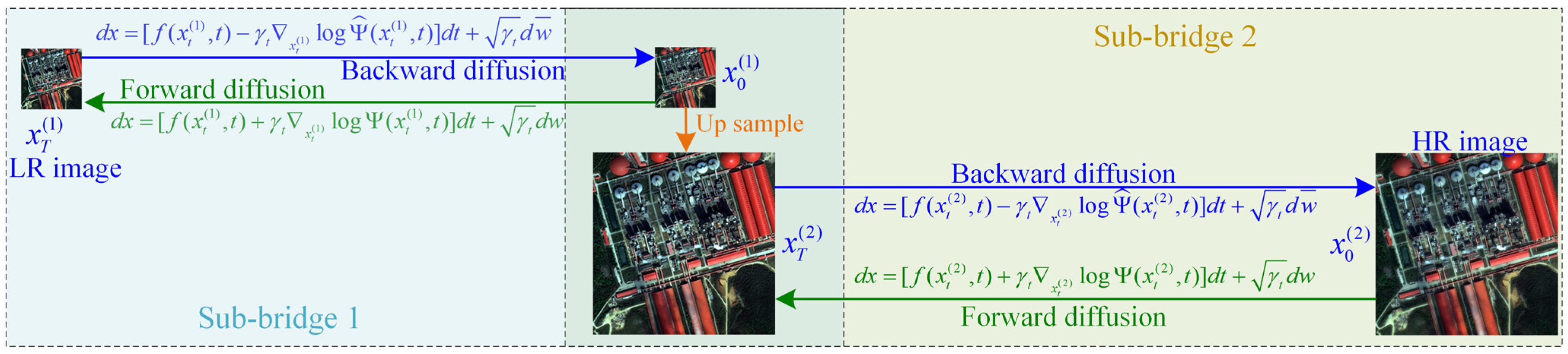
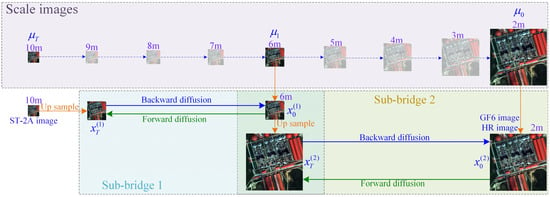
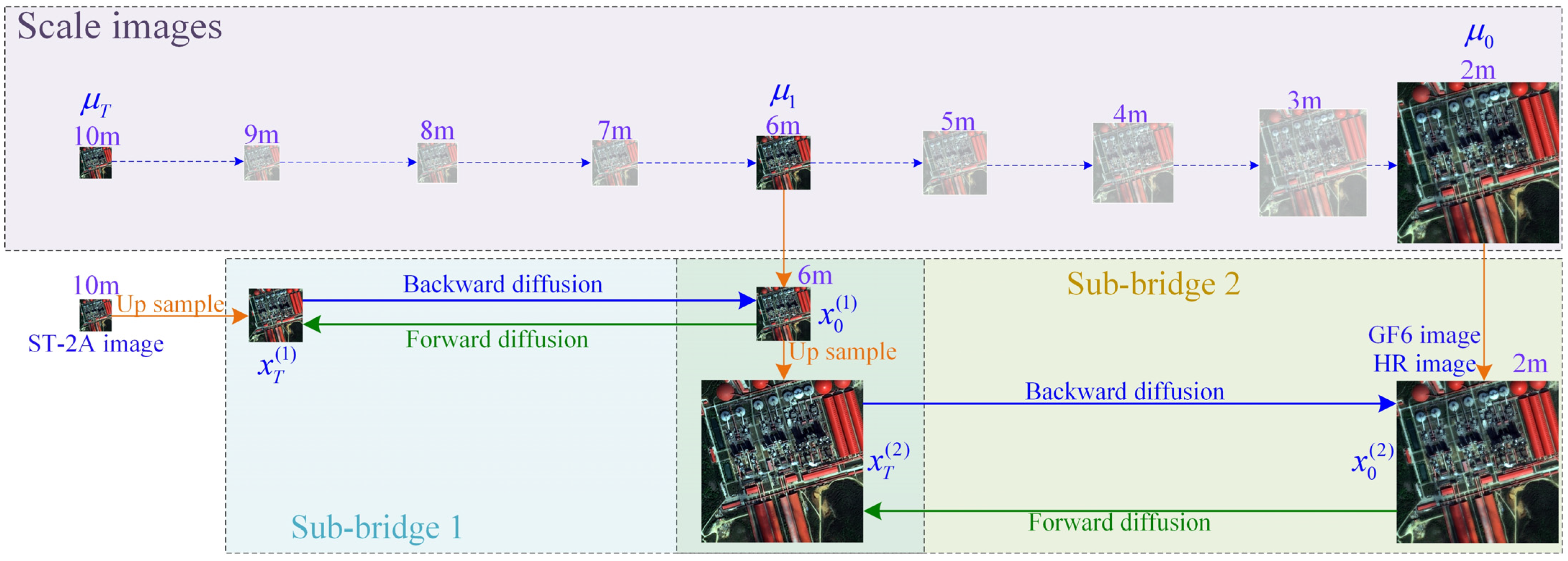
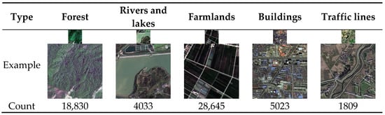
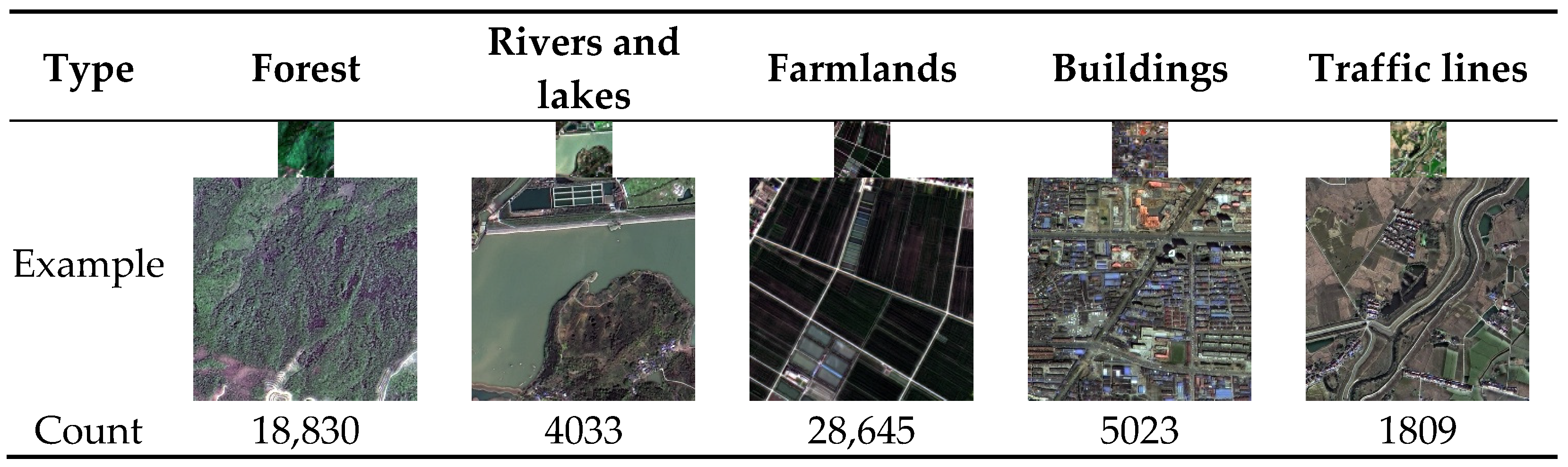
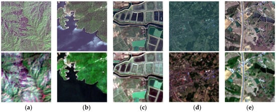
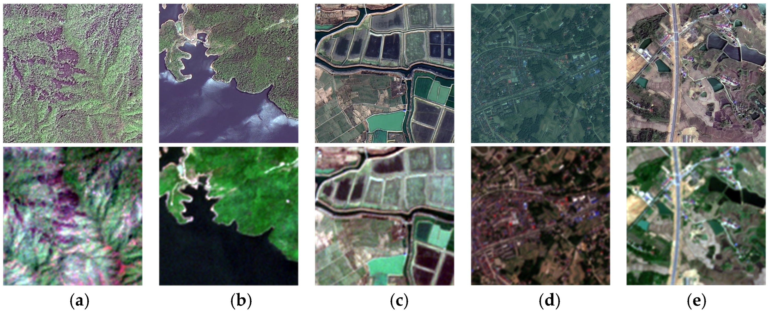
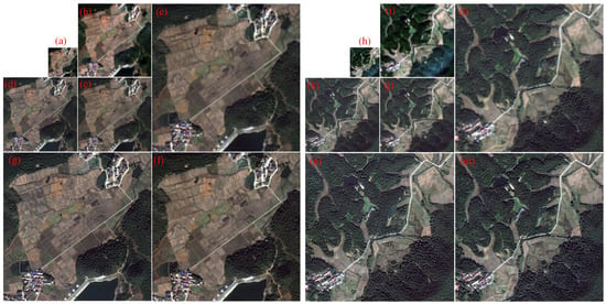
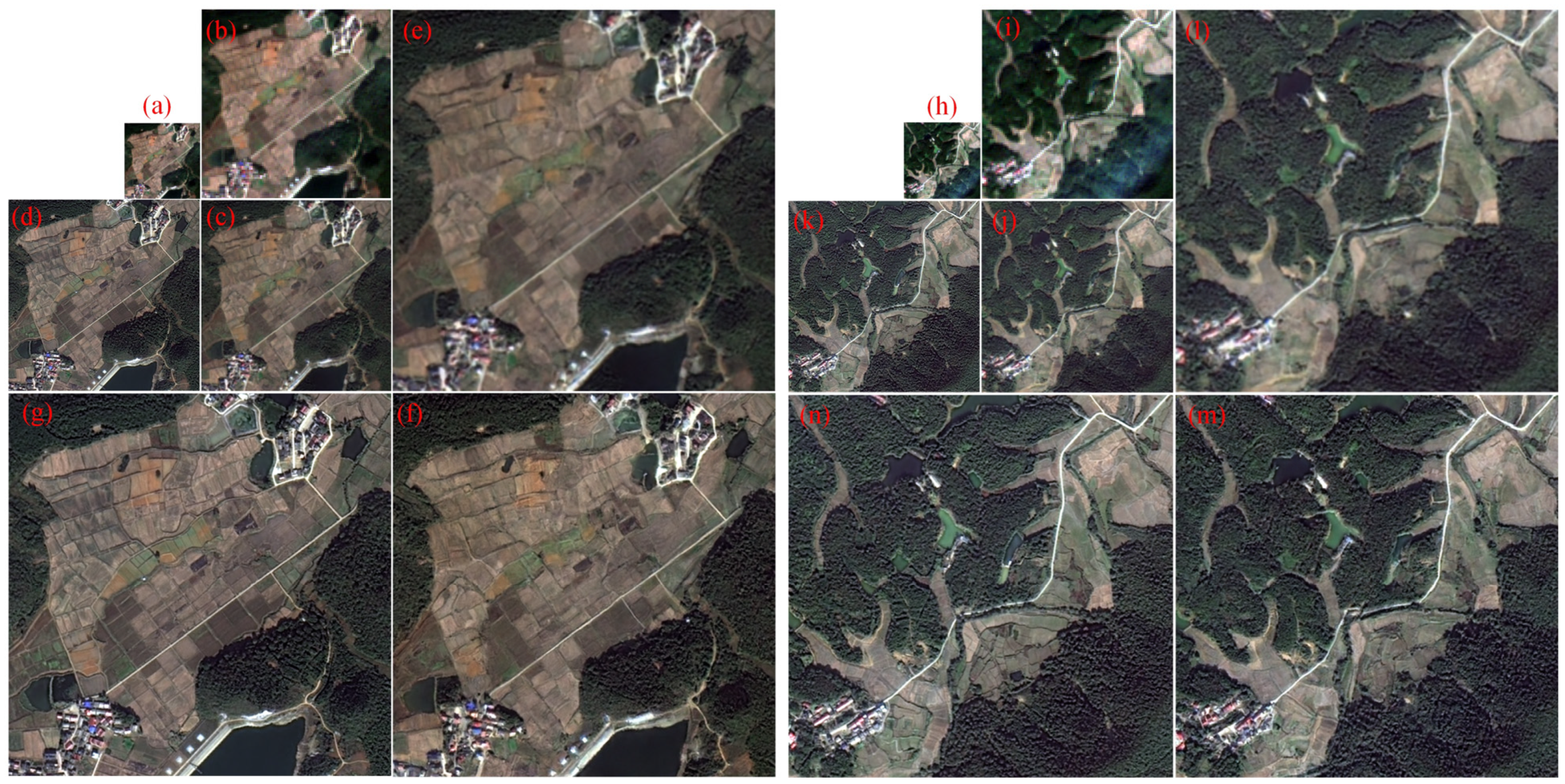
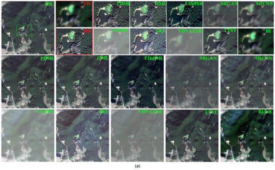
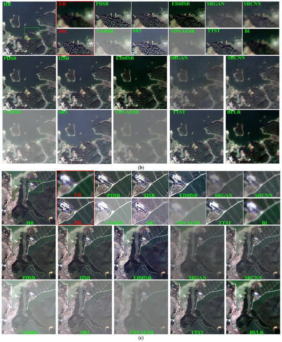
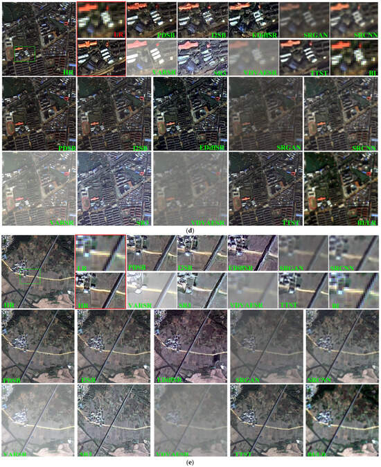
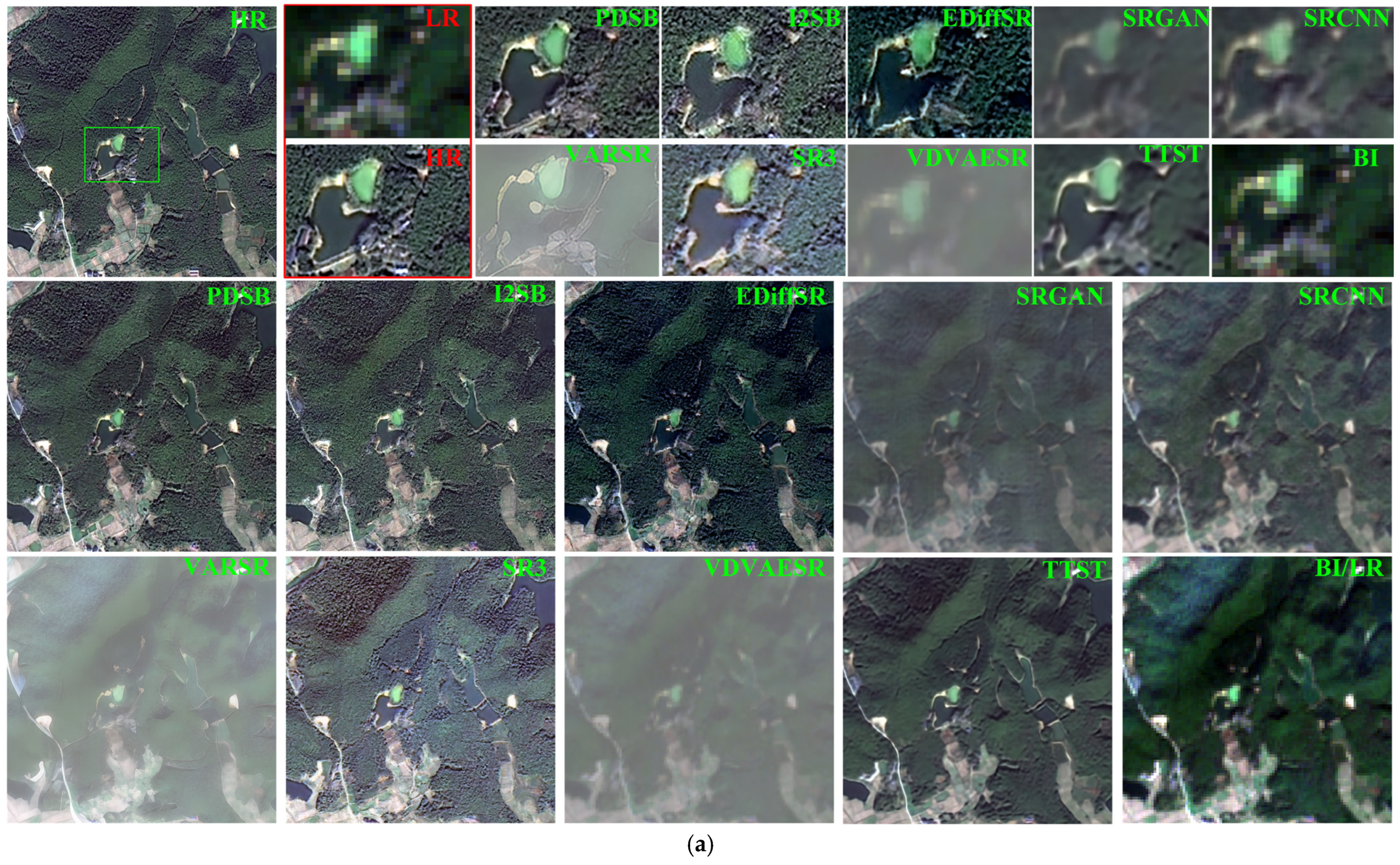
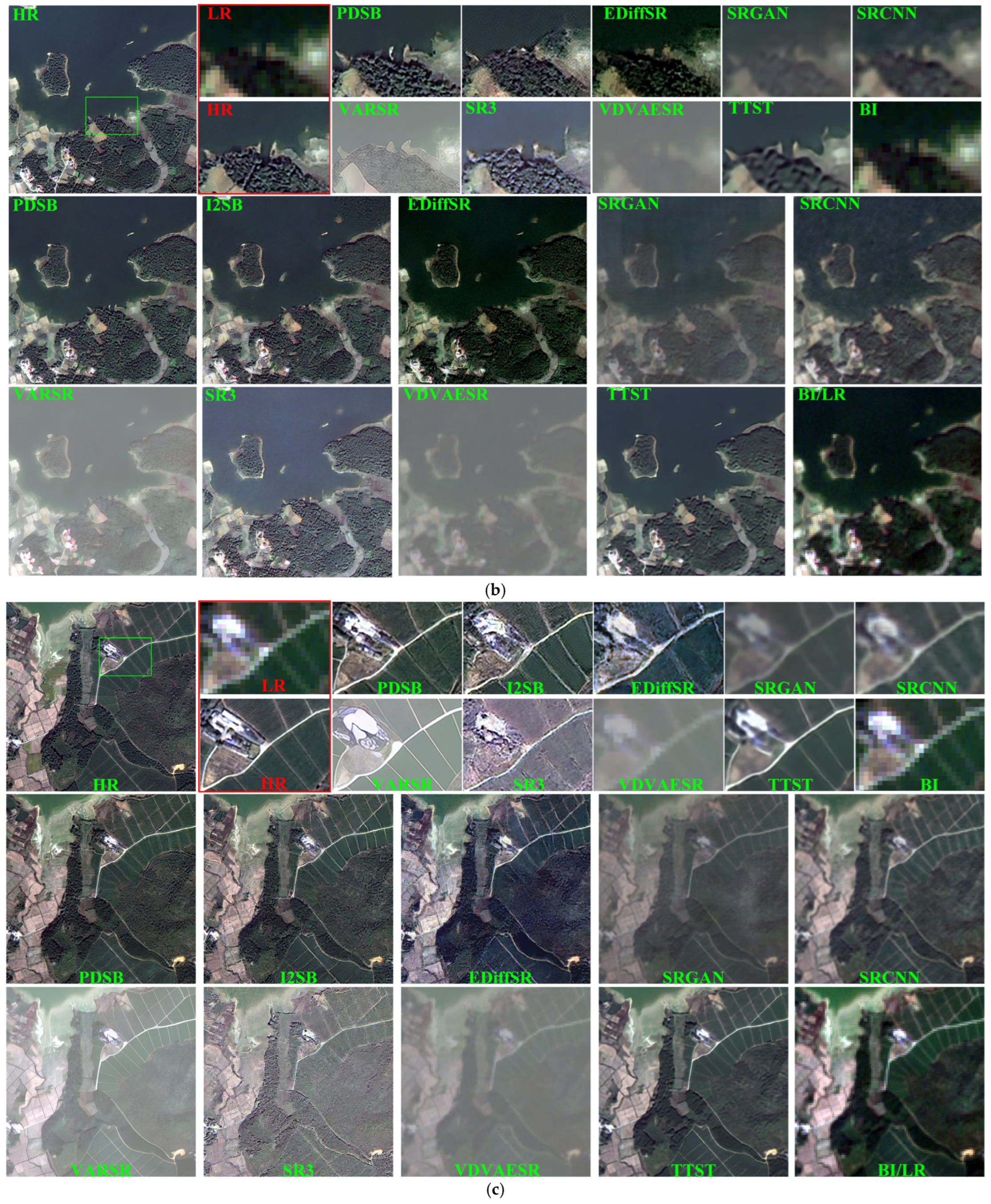
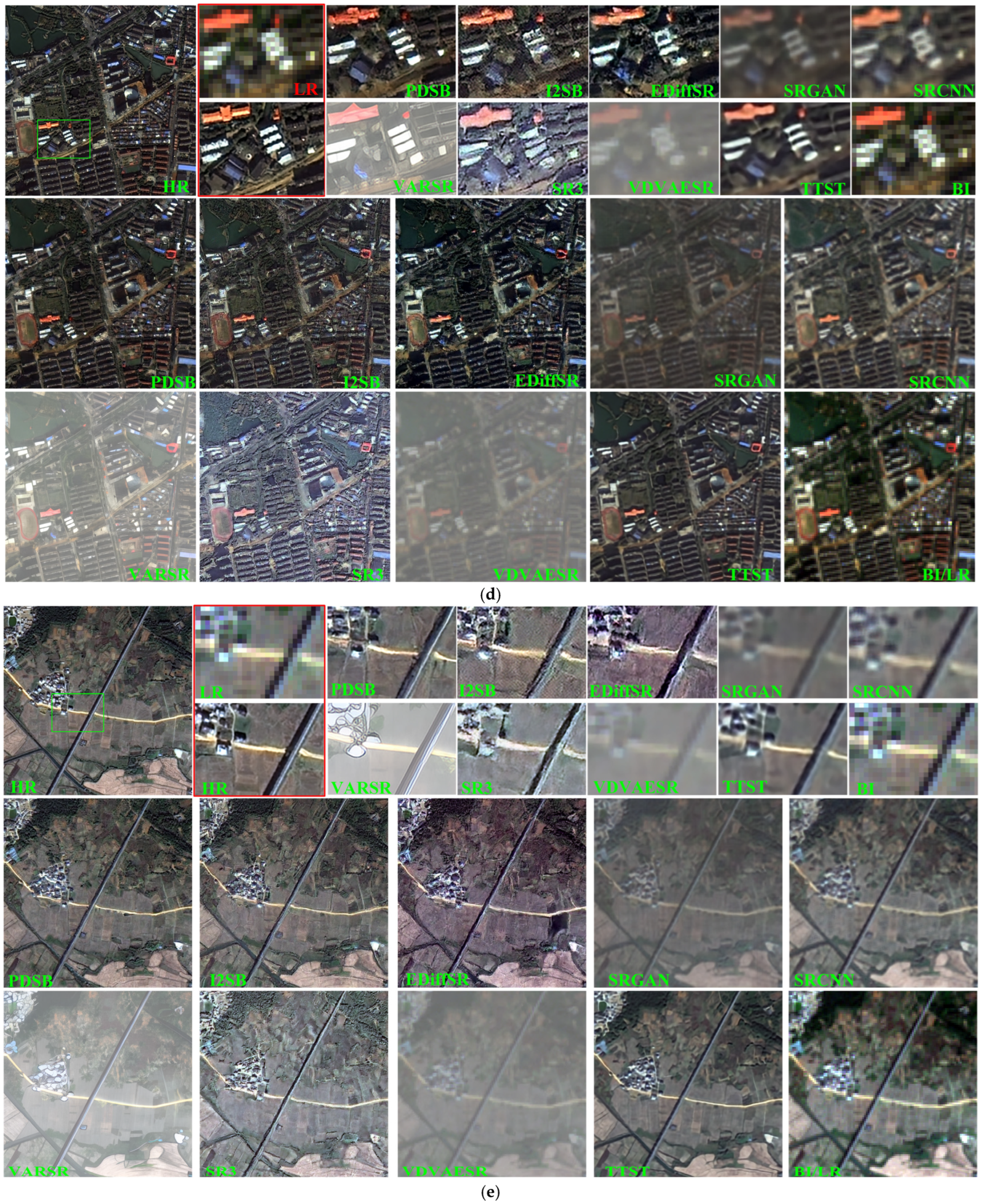
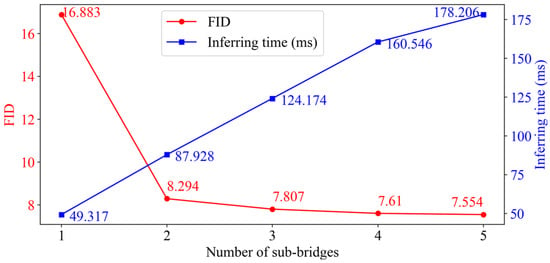
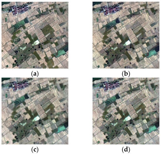
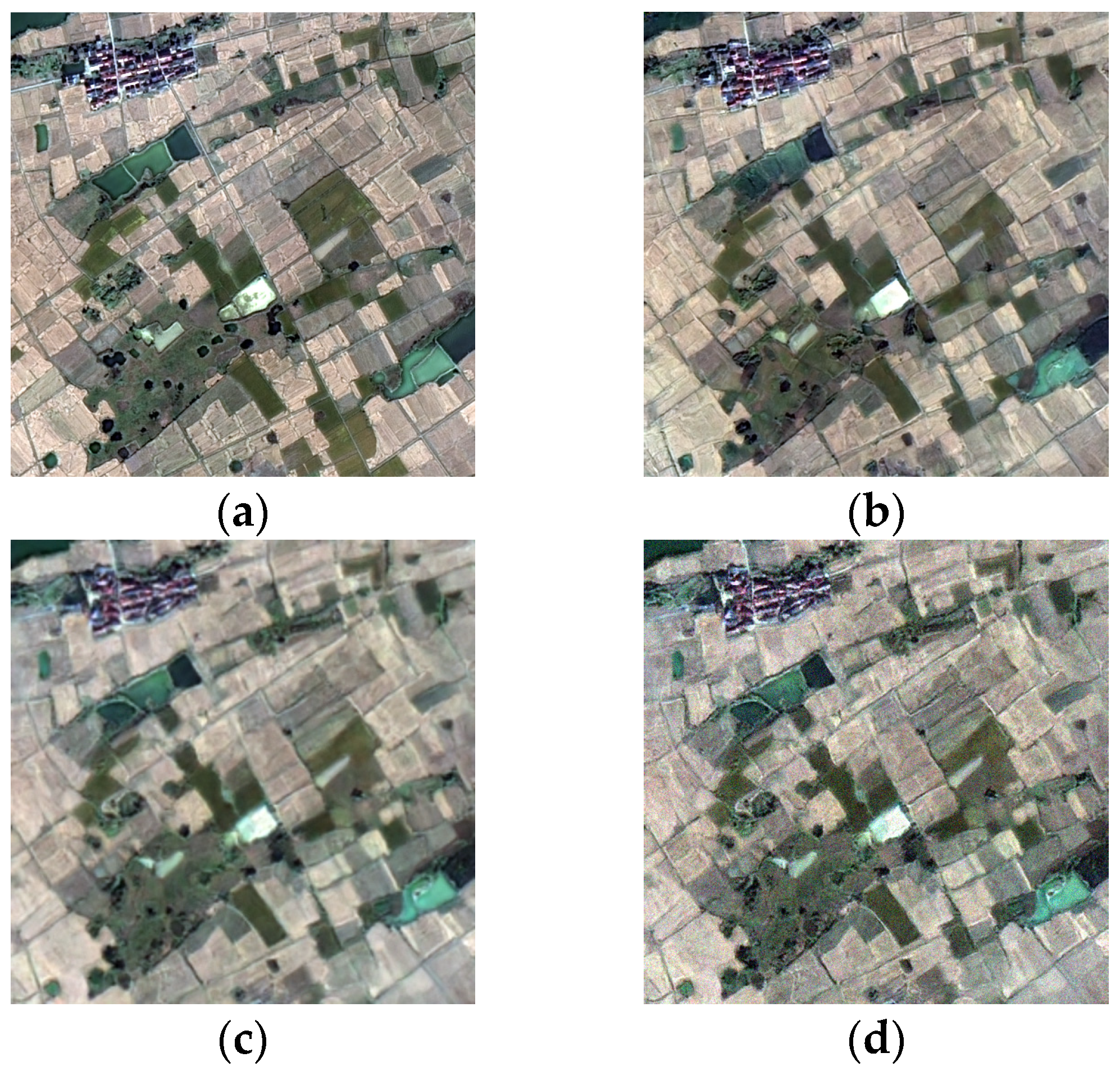
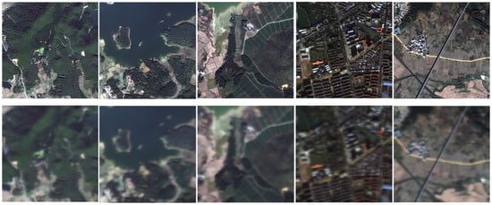
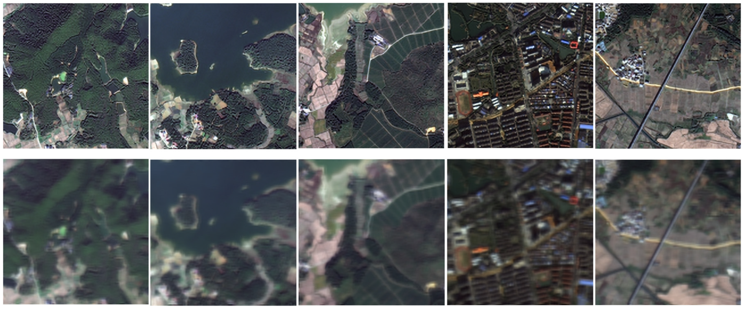

Disclaimer/Publisher’s Note: The statements, opinions and data contained in all publications are solely those of the individual author(s) and contributor(s) and not of MDPI and/or the editor(s). MDPI and/or the editor(s) disclaim responsibility for any injury to people or property resulting from any ideas, methods, instructions or products referred to in the content. |
© 2026 by the authors. Licensee MDPI, Basel, Switzerland. This article is an open access article distributed under the terms and conditions of the Creative Commons Attribution (CC BY) license.