


Highlights
What are the main findings?
- •
- CAS, built upon deformable convolution, further explores its application in hyperspectral unmixing. It adopts customized initial shapes and numbers of sampling points, and imposes constraints and regularization terms to adjust sampling positions for spatial feature extraction.
- •
- SE module is placed along the spectral dimension to strengthen the representation of spectral information and achieve compatibility with the spatial CAS branch.
- •
- Skip connection compensates for the detailed information loss after a series of convolutions and nonlinear transformations in the dual branches, and participates in the direct estimation of abundance maps.
What are the implications of the main findings?
- •
- The net supports hyperspectral unmixing in scenes with irregular boundaries and fragmented material distributions.
- •
- The joint objective combines reconstruction fidelity, spectral-shape agreement, and offset regularization to guide spectral reconstruction and spatial sampling during unsupervised unmixing.
Abstract
Regular convolution is widely used in spectral–spatial unmixing networks to aggregate neighborhood information, but its fixed sampling grid cannot readily follow irregular material boundaries or elongated structures and may introduce heterogeneous pixels whose compositions differ from that of the central pixel. This study presents DB-CASSE-Net, a dual-branch hyperspectral unmixing network that combines constrained adaptive spatial sampling with spectral feature enhancement. The spatial branch learns position-dependent offsets from configurable initial sampling geometries. A hyperbolic-tangent mapping bounds the displacement range, while magnitude and spatial-smoothness regularizers suppress excessive drift and abrupt local changes. In parallel, the spectral branch uses pointwise convolutions and an identity-initialized squeeze-and-excitation mechanism to recalibrate latent spectral channels adaptively. Features from the two branches are fused, and a spectral skip connection restores fine-grained information from the original spectral signatures that may be attenuated by successive nonlinear transformations. The resulting abundance responses satisfy nonnegativity and sum-to-one constraints, and a nonnegative linear decoder reconstructs the hyperspectral image, enabling unsupervised joint estimation of endmembers and abundances. Experiments on Jasper Ridge, Samson, and Urban show that DB-CASSE-Net achieves the lowest mean abundance RMSE and mean endmember SAD among the compared methods on Jasper Ridge and Urban, and the second-lowest mean abundance RMSE on Samson.
1. Introduction
Hyperspectral images (HSI) record surface reflectance in tens to hundreds of contiguous narrow bands, so that each pixel contains both a spatial location and a detailed spectral signature. This integrated spatial–spectral representation supports material identification and fine-grained analysis of ground objects and has been widely used in agricultural remote sensing, mineral identification, and environmental monitoring [1,2]. However, because of limited spatial resolution and the complexity of ground targets, a single observed pixel often contains the combined responses of multiple materials when the sensor footprint covers several objects or when light undergoes multiple scattering in a complex medium. These mixed pixels substantially complicate the interpretation of remote-sensing imagery [3]. Hyperspectral unmixing (HU) decomposes each mixed pixel into the spectral signatures of pure materials, termed endmembers, and estimates the proportion of each endmember in the pixel, termed abundance [4].
Conventional unmixing models are generally divided into the linear spectral mixture model (LSMM) and nonlinear spectral mixture models (NSMM). The LSMM represents an observed spectrum as a linear combination of endmember spectra and has received extensive attention because of its clear physical interpretation, manageable parameterization, and compatibility with abundance constraints [5]. Representative approaches include geometric methods [6,7,8], statistical methods [9], the sparse-regression method SUnSAL [10], and matrix-factorization methods [11,12]. NSMMs account for nonlinear spectral mixing caused by physical interactions among ground materials, such as photon transport and atmospheric scattering, and include intimate and multilayer mixing models [13,14]. Although these classical models are interpretable, their performance often depends on how well pure-pixel assumptions, spectral libraries, probability distributions, or structural priors match the actual scene. They may also be affected by nonconvex optimization, parameter selection, and initialization, limiting their ability to exploit latent data correlations for more accurate estimation [15].
Compared with physical models and shallow neural networks, deep learning offers data-driven spectral and spatial feature learning for a range of remote sensing tasks [16,17,18]. For hyperspectral anomaly detection, Wang et al. [19] proposed FTSGAN, which learns an adversarial mapping from fractional Fourier-domain representations to background spectra to improve background–anomaly discrimination. Wang et al. [20] developed PDBSNet, combining blind-spot reconstruction with pixel-shuffle downsampling to favor background reconstruction while suppressing anomaly reconstruction. In hyperspectral unmixing, deep networks can learn spectral mixing patterns directly and thereby improve unmixing accuracy [21]. Deep learning-based unmixing has therefore become an active research area [22]. Autoencoders (AE) are particularly suitable because their structure corresponds naturally to the LSMM: the encoder maps a high-dimensional spectrum to a low-dimensional latent vector that can be interpreted as abundance, while the weight matrix of a linear decoder reconstructs the spectrum and its columns can be interpreted as endmembers. Palsson et al. [23] demonstrated the feasibility of an asymmetric autoencoder for blind unmixing and showed that a spectral-angle-distance (SAD) objective benefits endmember-shape recovery. Ozkan et al. [24] strengthened endmember extraction and abundance estimation using a spectral-angle-related loss and a sparsity constraint. Qu et al. [25] introduced uDAS, which combines untied encoder–decoder weights, a denoising constraint, and an penalty on the encoder weights to reduce redundant endmembers. These early methods processed spectra pixel by pixel and learned nonlinear interband relationships, but did not fully exploit spatial correlations among neighboring pixels.
Convolutional neural networks (CNN) were subsequently introduced into autoencoder-based unmixing to exploit spatial structure jointly with spectral information. Palsson et al. [26] proposed an early convolutional autoencoder for blind spectral–spatial unmixing, using convolutional encoders to extract joint features from HSI patches so that neighborhood information contributed to abundance estimation. Hua et al. [27] developed gated autoencoder architectures that adaptively controlled the contribution of spatial features according to local correlations, thereby preserving the dominant role of spectral information. These studies showed that properly used spatial neighborhoods can improve abundance consistency within homogeneous regions. Spatial information is not always beneficial, however: excessive aggregation may blur abundance boundaries when a neighborhood crosses a material boundary or contains isolated objects. Xu et al. [28] likewise noted that uniform convolutional smoothing over an entire image can ignore within-scene differences and cause oversmoothing; they therefore proposed a global–local smoothing autoencoder to describe local homogeneity and global self-similarity separately. The central challenge in spectral–spatial unmixing is thus not merely whether spatial information is used, but how effective neighbors are selected according to the local material distribution while suppressing interference from heterogeneous pixels.
Beyond conventional reconstruction-based autoencoders, adversarial learning and masked modeling have also been explored for hyperspectral unmixing. Jin et al. [29] introduced AAENet, which incorporates abundance priors reflecting local spatial correlations through adversarial training. Guo et al. [30] combined manifold regularization with an adversarial autoencoder and Fourier convolution to preserve local structure and integrate local and global contextual information. Xu et al. [31] developed MsCM-Net, which combines a mixed-region masking strategy with a multiscale convolutional autoencoder to improve robustness to interference in highly mixed regions. These studies broaden the learning strategies available for unmixing and highlight the importance of incorporating spatial structure and task-specific priors into reconstruction-based models.
Transformer architectures and multi-head self-attention have recently provided an alternative means of modeling nonlocal dependencies. Unlike local convolutions operating within fixed windows, self-attention evaluates correlations between positions from the input features and thus expands the spatial context. Ghosh et al. [32] proposed DeepTrans-HU (TAEU), which embeds a Transformer in the latent space of a convolutional autoencoder to model long-range relationships among image patches. Yang et al. [33] combined shifted-window self-attention with a U-shaped network in UST-Net to establish cross-window spatial connections during multiscale feature extraction. Tao et al. [34] introduced the abundance-guided spectral–spatial network A2SN and its attention-enhanced variant A2SAN, which use different kernels to extract spectral and spatial features and an abundance-guidance mechanism to reduce dependence on conventional endmember initialization. More recent studies have addressed noise suppression, endmember variability, and coordinated local–global modeling. Related attention-based architectures have also been developed for hyperspectral unmixing [35]. Tao et al. [36] integrated deep denoising, autonomous endmember inversion, and spectral–spatial attention in an end-to-end network to reduce sensitivity to noise and decoder initialization. Gao et al. [37] combined cascaded encoders with a variational-autoencoder-based generative model for adaptive spectral–spatial fusion while explicitly accounting for endmember variability. Cui et al. [38] used spectral–spatial similarity in a nested Transformer to represent both local pixel relations and global context, mitigating the loss of pixel-level continuity caused by nonoverlapping patches. Cao et al. [39] related subspace attention and iterative shrinkage-thresholding to feature compression and sparsification, respectively, to improve mechanistic interpretability. Across these architectures, local feature aggregation remains important for spatial–spectral representation learning. Conventional convolutions sample fixed locations relative to each output pixel, which limits their ability to follow irregular material boundaries and narrow structures. Deformable convolutional networks introduce learnable sampling offsets [40], while AKConv allows configurable sampling-point counts and initial geometries [41]. Such sampling flexibility has also been explored in hyperspectral unmixing. Qu et al. [42] incorporated multiscale deformable convolutions into the neighborhood spatial offset Mamba branch of DGMNet to capture local spatial structures. Such approaches extend the flexibility of neighborhood aggregation and motivate further investigation into how sampling displacements and their spatial variation can be controlled during unmixing.
Alongside the selection of spatial neighbors, abundance estimation also depends on how each pixel’s own spectrum contributes to the prediction. As neighborhood information is incorporated through successive feature transformations, a direct path from the input spectrum can provide complementary pixelwise information to the resulting spatial–spectral representation. The placement of this path determines where the two sources of information interact. Connecting the original spectra to abundance logits allows their projected responses to be combined with the fused features before abundance normalization.
Motivated by these observations, this study proposes DB-CASSE-Net, a dual-branch hyperspectral unmixing network that integrates constrained adaptive spatial sampling (CAS) with spectral enhancement (SE). The network combines controlled spatial feature aggregation with pixelwise spectral representation learning through a dual-branch (DB) architecture. Its main contributions are as follows:
- An AKConv-based constrained adaptive spatial sampling (CAS) module is developed for hyperspectral unmixing. Building on the configurable sampling geometries and learnable offsets of AKConv, CAS introduces a hyperbolic-tangent displacement bound together with offset-magnitude and spatial-smoothness regularization. These additions respectively limit displacement from the initial sampling positions, penalize excessive drift, and discourage abrupt spatial variations in the offset field. Within the spatial branch, CAS therefore enables location-dependent resampling of learned spatial features while imposing explicit control over the extent and spatial variation in sampling adjustments.
- A spectral enhancement (SE) component is constructed by combining identity-initialized channel recalibration with a spectral skip connection. It adopts the channel-dependency modeling mechanism of squeeze-and-excitation to recalibrate pixelwise spectral features [43]. Unlike conventional sigmoid gating, the channel-expansion layer is initialized with zero weights and biases and followed by a doubled sigmoid mapping, yielding unit channel weights at initialization and subsequently allowing both feature attenuation and amplification. A complementary pointwise spectral skip connection maps the original input spectra directly to abundance logits, providing a spectral information path that bypasses the intermediate feature transformations. Together, these designs combine adaptive recalibration of latent spectral channels with direct input-spectrum information for abundance estimation.
- A dual-branch (DB) unmixing architecture is established to integrate constrained spatial sampling and spectral enhancement. The spatial branch aggregates local context through CAS, whereas the spectral branch learns interband representations through pointwise convolutions and channel recalibration. Their outputs are concatenated and projected to form a joint spectral–spatial abundance representation, which is combined with the spectral skip response before softmax normalization. A nonnegative linear decoder reconstructs the input image from the estimated abundances and endmembers. This architecture brings the complementary spatial and spectral representations into a common reconstruction objective while enforcing abundance nonnegativity and the sum-to-one constraint.
The remainder of this paper is organized as follows. Section 2 presents DB-CASSE-Net, including its architecture, constrained adaptive spatial sampling, spectral enhancement, and training objective. Section 3 examines the learned sampling behavior and evaluates unmixing performance on the Jasper Ridge, Samson, and Urban datasets. Section 4 summarizes the main findings, limitations, and future research directions.
2. Materials and Methods
2.1. Linear Spectral Mixture Model
DB-CASSE-Net is formulated under the linear spectral mixture model and therefore does not explicitly model multiple reflections or interactions among ground materials. The LSMM is expressed as follows:
where Y is the observed hyperspectral data with L spectral bands and N = H × W pixels; M is the endmember matrix containing P endmembers; A is the abundance matrix; and E represents additive noise. To ensure physically meaningful estimates, both M and A are nonnegative (ANC), and every abundance vector sums to one (ASC). The symbols 1P and 1N denote all-ones column vectors of lengths P and N, respectively.
In autoencoder-based blind unmixing, the low-dimensional encoder output is interpreted as abundance, and the weights of the linear decoder are interpreted as endmember spectra. The corresponding process is written as
Here, the functions in Equations (2) and (3) denote the encoder and decoder with their respective parameter sets; and are the estimated abundance and endmember matrices; and is the reconstructed HSI. The network is optimized using reconstruction objectives and offset regularization, enabling unsupervised joint estimation of endmembers and abundances.
2.2. Overall Architecture of DB-CASSE-Net
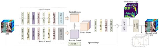
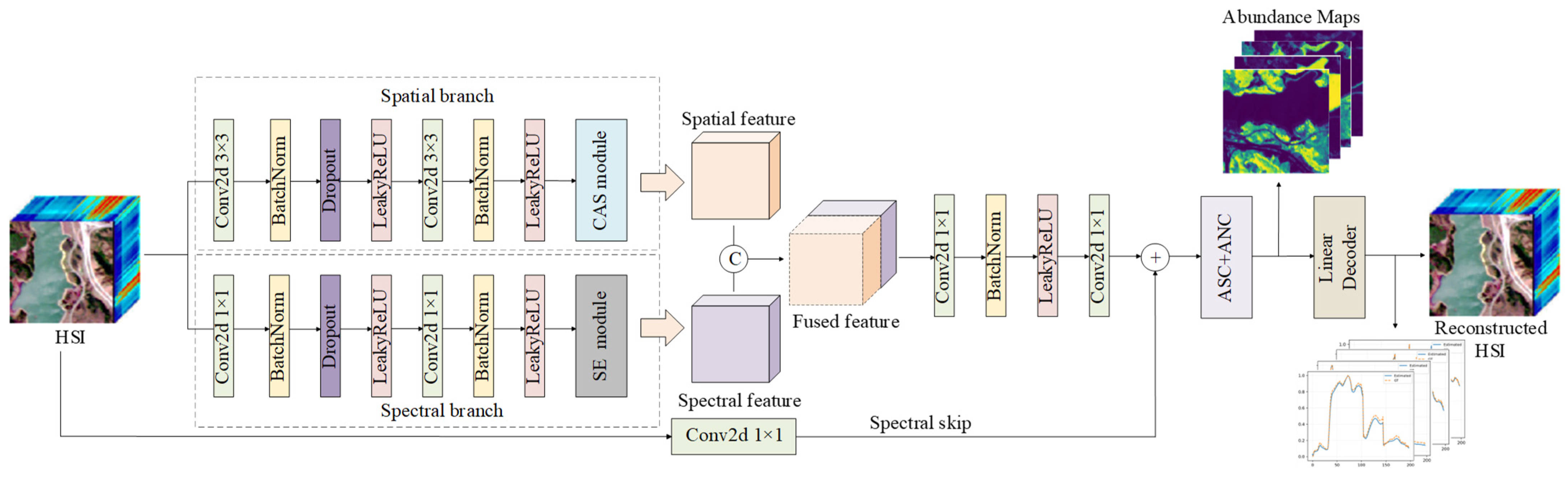
DB-CASSE-Net comprises a dual-branch spectral–spatial encoder, a spectral skip connection, and a linear decoder. The spatial branch first extracts local neighborhood information using regular convolutions and then adjusts the sampling locations using a constrained adaptive spatial-sampling module. The spectral branch extracts pixelwise spectral features, models interband relationships at each pixel, and recalibrates the resulting responses through channel attention. The branch features are concatenated and compressed to form the main abundance response, while the spectral skip path supplies spectral detail directly from the original HSI. Their responses are added to estimate abundances. Finally, the trainable nonnegative endmember matrix reconstructs the HSI through a linear decoder, completing joint unmixing. Figure 1 presents the architecture, and Table 1 lists the branch configurations.
Figure 1.
Architecture of DB-CASSE-Net.
Table 1.
Configuration of the two encoder branches.
2.2.1. Spatial Branch
The spatial branch contains two convolutional layers followed by a constrained adaptive spatial-sampling convolutional module (CAS). Batch normalization accelerates convergence, dropout after the first convolution reduces overfitting, and LeakyReLU preserves gradient propagation in the negative domain while increasing nonlinearity. Both regular convolutions use 3 × 3 kernels. The channel dimension is mapped from L to 128 and then to 64, combining the central pixel with its neighbors to form an initial spatial representation. Reflection padding maintains the spatial size at H × W. For compact notation, a convolutional block is defined as
where the asterisk denotes convolution, Wk×k denotes the kernel parameters, BN(⋅) is batch normalization, and ϕ(⋅) is the activation function. The initial spatial feature after the two regular convolutional layers is
The two 3 × 3 convolutional blocks produce a 64-channel feature map that retains the original spatial dimensions. These features provide local neighborhood context for offset prediction. CAS resamples contextual features produced by the preceding convolutions. Its displacement bound controls the extent of each sampling adjustment, while magnitude and smoothness regularization guide the learned offset field.
Let a standard two-dimensional convolution sample an input feature at location p0 according to a predefined set of K regular coordinates. Its output is
where rk is the fixed displacement of the k-th sampling point from the center, and wk is the corresponding convolution weight. Because rk is identical at every spatial position, a regular convolution cannot adapt its sampling extent to changes in object boundaries, shapes, or scales. Deformable convolution instead predicts a two-dimensional offset Δpk for every sampling point, so that the coordinates vary with the input features:
The displaced coordinates are generally noninteger, so their feature values are obtained by bilinear sampling. AKConv further generalizes the conventional k × k grid to a configurable set of K sampling points and permits different initial geometries according to the task. The initial sampling set is defined as
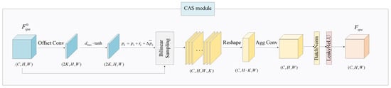
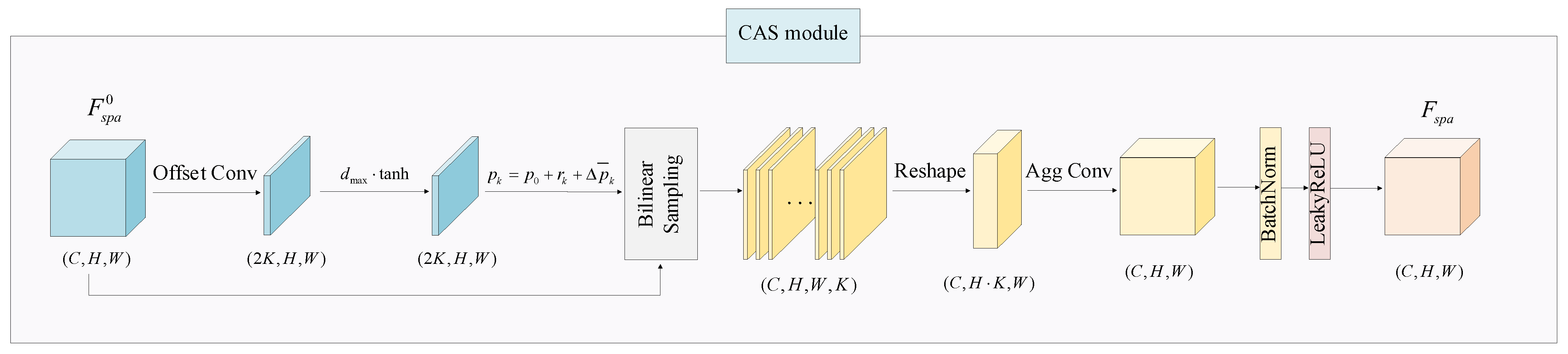
Each sampling point can therefore learn a position offset from its initial coordinate. This mechanism provides flexible control over both the number and the initial arrangement of sampling points and supports finer sampling of different local structures. When adaptive sampling is applied to the spatial feature map, large displacements may draw features from distant neighborhoods, while abrupt spatial variations in the offsets may produce sharply different sampling patterns at adjacent locations. DB-CASSE-Net therefore introduces displacement bounding and offset regularization into the AKConv-based sampling mechanism to control these adjustments (Figure 2).
Figure 2.
Convolutional module with constrained adaptive spatial sampling.
An offset-prediction convolution first generates raw offsets from the initial spatial feature , after which a hyperbolic-tangent function limits the maximum displacement along each coordinate axis:
In Equation (9), indicates a restricted offset field, dmax is the maximum displacement permitted along one coordinate axis. In implementation, the maximum displacement bound dmax is set to 1.0 pixel for the Jasper Ridge and Samson datasets, and 2.0 pixels for the Urban dataset to accommodate its higher spatial complexity and fragmented distributions. The actual coordinate of the k-th sampling point at p0 is
The weights and bias of the offset-prediction convolution are initialized to zero. The model therefore begins with the preset sampling geometry and then gradually learns location adjustments from local structure. At a noninteger pk sampling position, the feature value is computed by bilinear interpolation from the four neighboring integer grid points:
In Equation (11), ℕ(pk) specifies the four integer positions adjacent to the sampling coordinates and G(⋅) represents the bilinear interpolation weights. Reflection-boundary handling reduces abnormal responses caused by zero padding at the image edges. The resampled features from the K points are then arranged sequentially and aggregated by a K × 1 convolution with stride K × 1 (Agg conv). The final spatial feature Fspa ∈ R64×H×W is
2.2.2. Spectral Branch
The spectral branch consists of two pointwise convolutional blocks followed by an SE channel-attention module. The two blocks map the L input bands to 128 and then 64 latent feature channels. Unlike the 3 × 3 convolutions in the spatial branch, the 1 × 1 convolutions mix channels at each spatial location without convolutional aggregation of neighboring pixels. Together with the nonlinear activations, they learn interband representations that complement the neighborhood-based spatial features. The initial spectral feature is expressed as
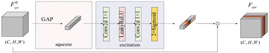
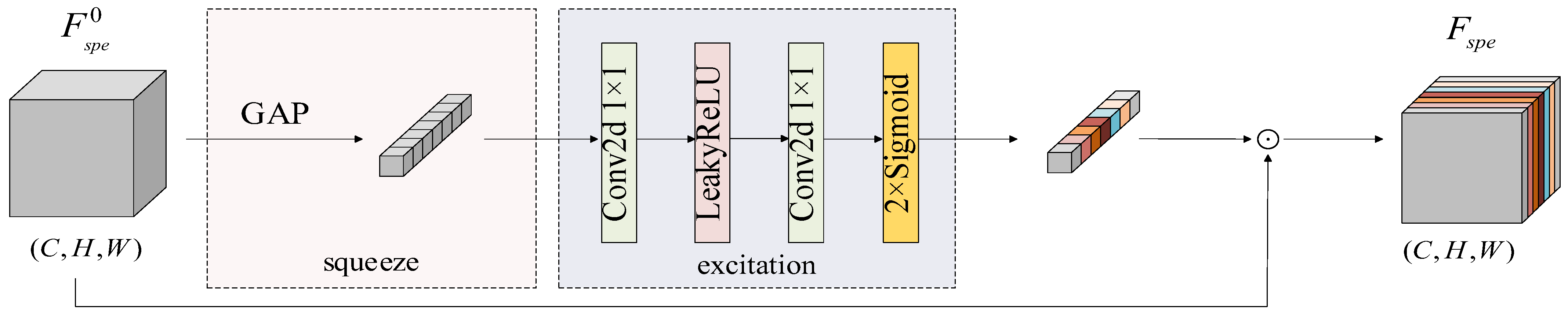
Each block in Equation (13) comprises pointwise convolution, batch normalization, and LeakyReLU activation, with dropout additionally applied in the first block. The resulting channels represent learned combinations of input bands rather than individual physical wavelengths. SE recalibrates the resulting latent channels before fusion, starting from unit channel weights and subsequently learning their relative contributions to reconstruction. Accordingly, spectral enhancement in this branch refers to interband feature learning and latent-channel recalibration; it does not explicitly model spectral-band continuity or local spectral structure. To adaptively weight these latent channels, an identity-initialized SE module is applied to , as illustrated in Figure 3. Global average pooling summarizes each channel over the spatial dimensions, and the resulting descriptors are transformed into channel weights through a bottleneck comprising channel reduction and expansion. These weights are shared across spatial locations and multiplied channelwise with to obtain the recalibrated feature Fspe. The weight-generation process and its identity initialization are described below.
Figure 3.
Identity-initialized channel-attention module used in the spectral branch (SE module).
Specifically, the expansion layer is initialized with zero weights and biases, and its output is passed through a doubled sigmoid mapping. The channel descriptor, recalibration weights, and output feature are defined as follows:
Here, z is the global channel descriptor. s contains the channel-attention weights. δ(⋅)and σ(⋅) denote LeakyReLU and sigmoid activation, respectively. ⊙ denotes channelwise multiplication. W1 and W2 are weight matrices and b1 and b2 are biases. Because W2 and b2 are initialized to zero, every channel weight equals one at the beginning of training and the spectral features are not perturbed by random gating. During training, the learned weights amplify or attenuate latent channels according to the reconstruction objective.
2.2.3. Spectral–Spatial Feature Fusion and Reconstruction
The spatial and spectral features are concatenated to form a 128-channel feature map. A 1 × 1 convolution followed by batch normalization and LeakyReLU reduces this map to 64 channels. A separate bias-free 1 × 1 convolution then projects the fused features to P abundance logits.
The spectral skip connection maps the L input bands directly to P logits through a 1 × 1 convolution whose weights and biases are initialized to zero. The skip output is therefore zero at initialization, and the initial abundances are determined by the fused-feature logits. During training, the skip parameters are optimized jointly with the main branch to learn an additional mapping from the input spectra to the abundance logits, where it shares the endmember-channel dimension of the fused response. This placement allows the original spectra to contribute directly to abundance prediction, after which a common softmax enforces nonnegativity and the sum-to-one constraint.
The estimated abundances are mapped back to the spectral domain by a bias-free linear decoder. Its endmember matrix is parameterized by applying Softplus to an unconstrained trainable matrix. The unconstrained parameters are initialized using the inverse Softplus of the prepared initial endmembers. For Samson and Urban, the endmember columns are additionally normalized to unit Euclidean norm at initialization and during each forward pass; this normalization is not applied to Jasper Ridge.
2.3. Loss Function
To ensure accurate reconstruction, a mean-squared-error (MSE) term measures the numerical difference between the reconstructed HSI and the original observation at every spatial position and spectral band:
MSE is sensitive to spectral magnitude, and by itself may not preserve spectral shape adequately. A pixelwise spectral angle distance (SAD) term is therefore used to emphasize shape agreement and improve unmixing stability:
Here, yi,j ∈ RL denotes the observed input spectrum at spatial location (i,j) and denotes its reconstructed counterpart. The indices i and j refer to image rows and columns, respectively. Averaging these pixelwise spectral angles over all N = H × W pixels gives
Adaptive sampling adjusts sampling locations dynamically from the input features. Excessive displacements may cross material boundaries, while rapid spatial changes in the offset field can destabilize sampling. Magnitude and spatial-smoothness constraints are therefore imposed jointly on the normalized offset field. The offset regularizer is defined as
In Equation (20), ∇h and ∇v represent the first-order differences in the horizontal and vertical directions, respectively. μ represent smooth term weights and the size is μ = 0.1. The first term limits displacement from the initial position, and the second promotes continuous offset fields between neighboring pixels. The offset regularizer is activated progressively through a coefficient ρ(t). At the beginning of training, ρ(t) = 0 so that the network first learns the basic spectral–spatial reconstruction relationship; it then increases to one to stabilize offset learning. For a total of T epochs and current epoch t, the schedule is
The total objective is therefore
where α, β, and λ are the weights of the MSE, SAD, and offset-regularization terms, respectively.
2.4. Experimental Design and Evaluation Protocol
DB-CASSE-Net was evaluated on three real hyperspectral datasets—Jasper Ridge, Samson, and Urban—and compared with VCA–FCLS [7,44], DAEN [45], CyCU-Net [46], TAEU [32], A2SN [34] and SSAF-Net [37]. VCA extracts endmembers and FCLS estimates abundances from those endmembers. DAEN, CyCU-Net, TAEU, and A2SN represent deep autoencoder, cascaded autoencoder, Transformer-based, and abundance-guided spectral–spatial unmixing frameworks, respectively. SSAF-Net combines cascaded encoders for adaptive spatial–spectral fusion with a variational-autoencoder-based generative model to account for endmember variability. For Jasper Ridge, Samson, and Urban, respectively, DAEN was trained for 100, 180, and 130 epochs at a learning rate of 0.005, and CyCU-Net was trained for 420, 480, and 300 epochs at learning rates of 0.008, 0.002, and 0.002. TAEU used a patch size of 5 and was trained for 240 epochs at a learning rate of 0.003 on all three datasets. A2SN estimated endmembers internally and was trained for 1000, 1000, and 300 epochs, respectively, at a learning rate of 0.001. Because unsupervised estimates are subject to channel-permutation ambiguity, a cost matrix was first constructed from the spectral angles between estimated and reference endmembers. The Hungarian algorithm then established a one-to-one endmember assignment, after which abundance channels were reordered consistently before the metrics were calculated. Abundance maps were displayed on a common range from 0 to 1, and each estimated and reference endmember was normalized individually before its spectral shape was compared. For endmember initialization, VCA, N-FINDR, and clustering-based algorithms are adopted for the Samson, Jasper Ridge, and Urban datasets, respectively. Table 2 lists the parameter settings. Accuracy was measured using root-mean-square error (RMSE), mean RMSE (mRMSE), SAD, and mean SAD (mSAD):
Table 2.
Dataset-specific training parameters.
In Equation (23), and Ap,n represent respectively the estimated abundance and the true abundance of the p-th endmember within the n-th pixel. In Equation (25), and mp represent respectively the p estimated endmember and the true endmember. Lower RMSE and SAD values indicate more accurate estimates. All SAD values are reported in radians.
3. Results and Discussion
3.1. Offset Fields and Adaptive Sampling Behavior
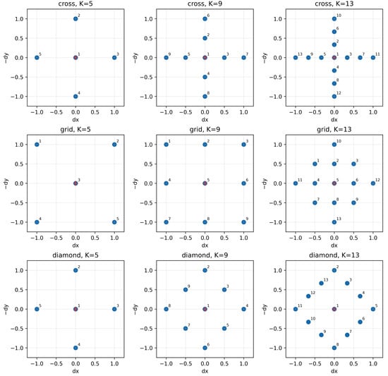
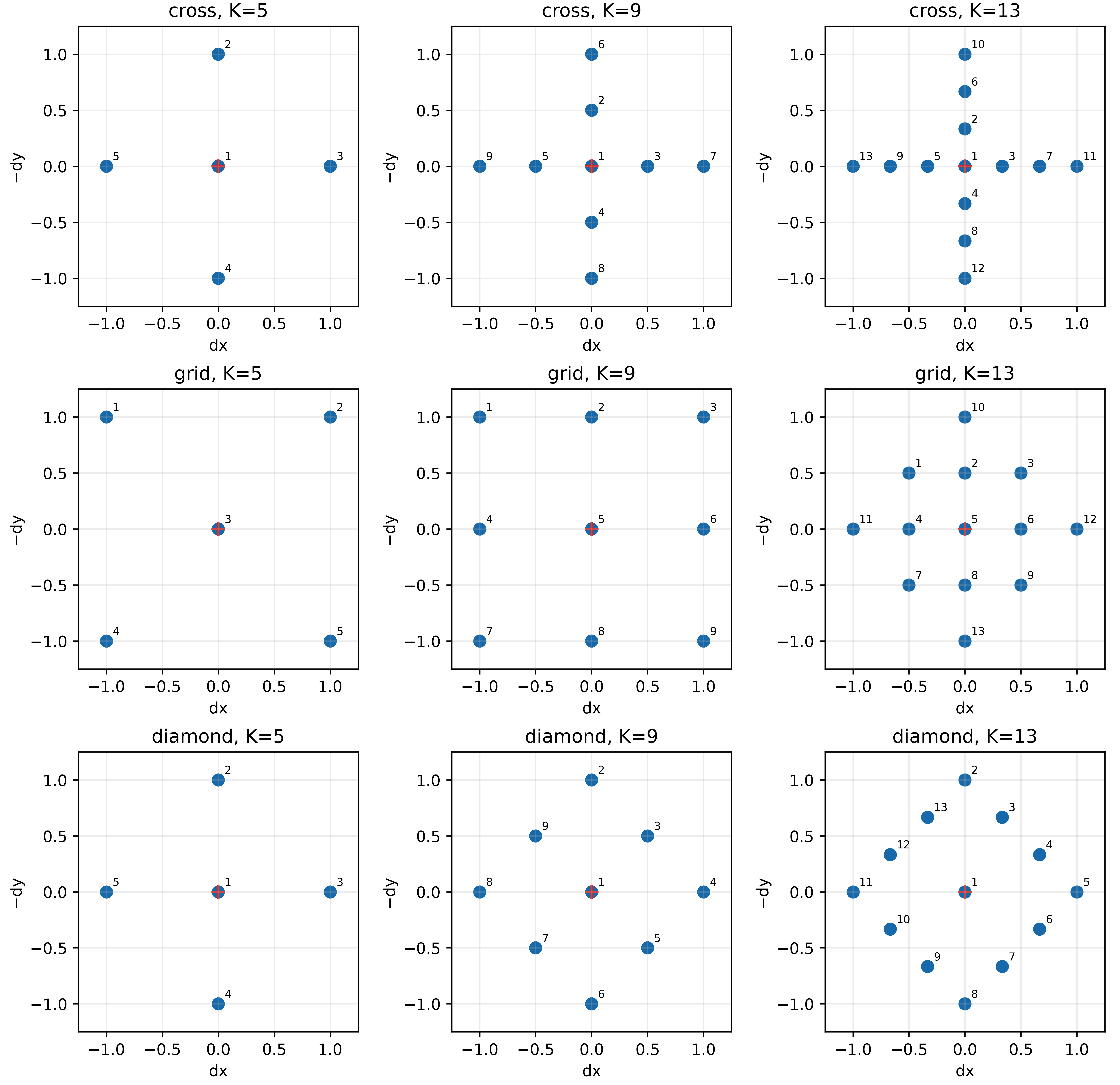
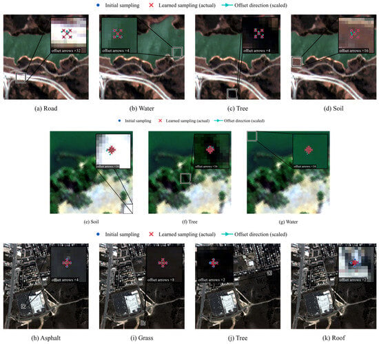
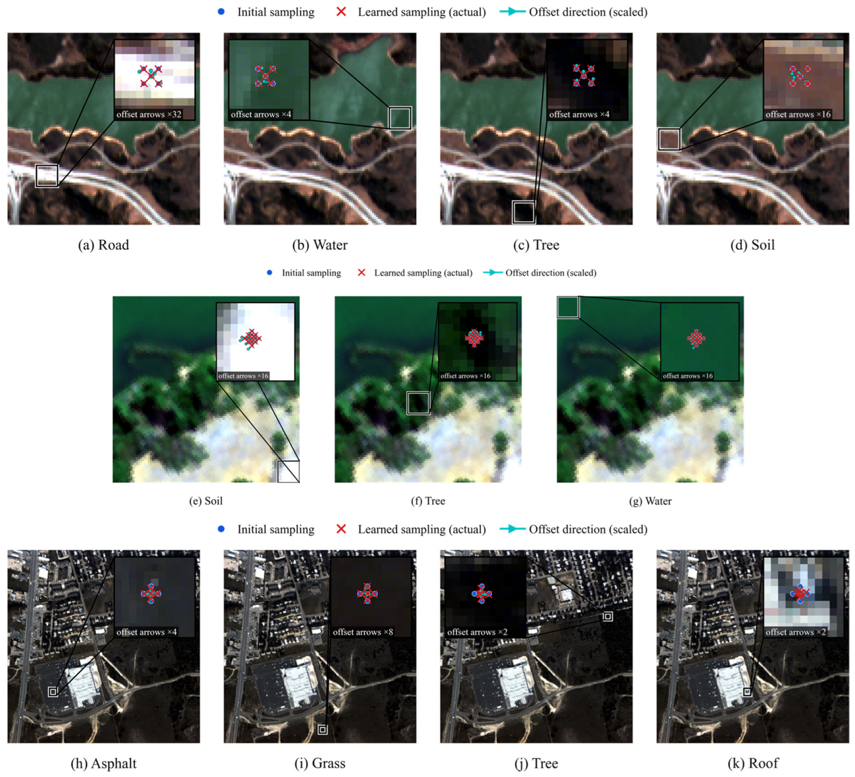
To examine the sampling behavior of CAS, we considered cross, grid, and diamond initial sampling layouts inspired by the configurable sampling strategy of AKConv, each with K = 5, 9, and 13 sampling points (Figure 4). The cross emphasizes horizontal and vertical coverage, the grid provides two-dimensional neighborhood coverage, and the diamond distributes sampling points along a diamond-shaped perimeter around the center. The cross and diamond layouts coincide when K = 5. Within each dataset, the layout and sampling-point count were evaluated while keeping the other training settings fixed, using a weighted combination of normalized abundance mRMSE, endmember mSAD, and reconstruction SAD, with respective weights of 0.4, 0.4, and 0.2. This criterion balances abundance and endmember estimation while also accounting for reconstruction fidelity. The selected configurations were grid K = 5 for Jasper Ridge, grid K = 13 for Samson, and cross K = 5 for Urban. Based on these configurations, Figure 5 and Figure 6 visualize the learned sampling adjustments at representative pixels and the image-wide offset fields, respectively. In Figure 5, blue dots denote the initial positions, red crosses denote the learned positions, and arrows indicate the offset direction from each initial point to its learned location.
Figure 4.
Preset numbers and initial geometries of the sampling points.
Figure 5.
Learned sampling offsets at representative pixels from (a–d) Jasper Ridge, (e–g) Samson, and (h–k) Urban.
Figure 6.
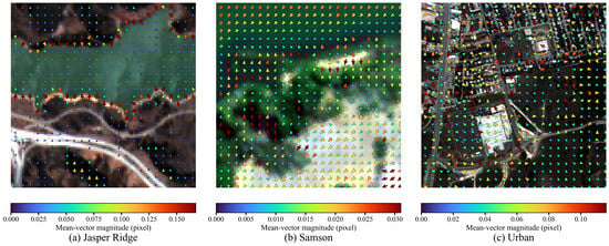
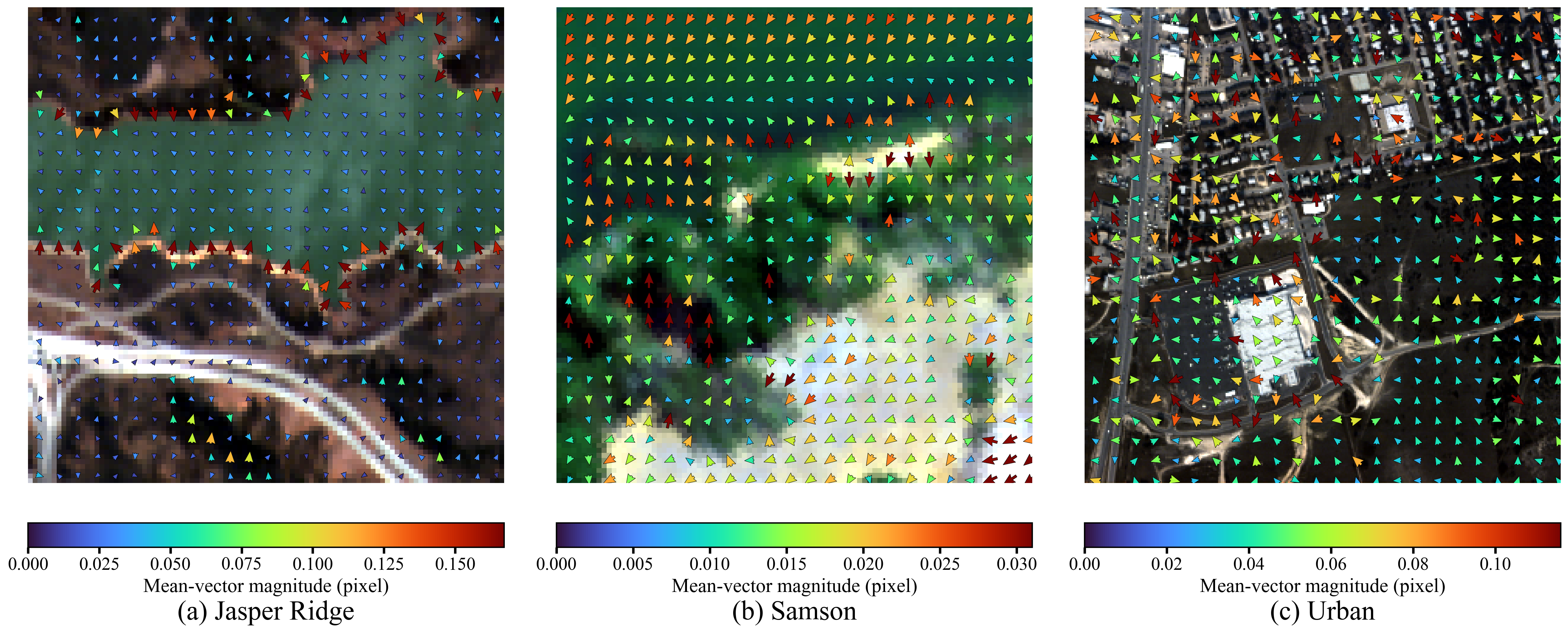
Image-wide offset directions and magnitudes for the three datasets.
In Figure 5a–d, the mean offset magnitudes for representative road and soil pixels are 0.0257 and 0.0331 pixel, respectively, so their sampling locations remain close to the initial grid. The corresponding means for water and tree increase to 0.1140 and 0.1254 pixel and show clearer directional corrections. The model therefore does not impose a uniform deformation on all pixels; instead, it changes aggregation locations according to local spectral–spatial responses. Given the many road, shoreline, and vegetation boundaries in this scene, larger offsets occur mainly in regions with stronger local composition changes.
In Figure 5e–g, the mean offset magnitudes for representative soil, tree, and water pixels range from 0.0358 to 0.0454 pixel, and none of the maximum offsets exceeds 0.0867 pixel. Although Samson uses the largest number of sampling points, the learned positions remain close to the initial grid. This behavior is consistent with the large homogeneous regions and strong spatial continuity of the dataset: the model mainly builds spatial constraints through dense but conservative neighborhood aggregation and does not require large displacements to expand its sampling range.
In Figure 5h–k, the mean offset magnitudes for representative asphalt, grass, tree, and roof pixels are 0.2070, 0.0909, 0.3380, and 0.3787 pixel, respectively. The maximum offsets for tree and roof reach 0.7050 and 0.5262 pixel. Urban exhibits the largest changes in offset magnitude and direction, particularly for tree and roof pixels, whose sampling points undergo strongly asymmetric adjustments.
Figure 6 displays the directional field obtained by averaging the offsets of all sampling points at each pixel. To prevent the directions of very small vectors from being dominated by numerical perturbations, arrows below the global 10th percentile were omitted. The mean vector magnitudes for Jasper Ridge, Samson, and Urban are 0.0382, 0.0157, and 0.0543 pixel, respectively. At each pixel, we also averaged the Euclidean offset magnitudes across the K sampling points. The spatial means of this map were 0.0713, 0.0269, and 0.1633 pixels, and its spatial maxima were 0.3484, 0.0631, and 0.4501 pixels for Jasper Ridge, Samson, and Urban, respectively. Samson has the smallest offsets and the greatest mean directional consistency, reflecting gradual adjustments within large homogeneous areas. Urban exhibited larger and more spatially variable offsets than the other two datasets. Jasper Ridge lies between these cases, with larger offsets occurring mainly near material boundaries and narrow structures.
Overall, constrained adaptive spatial sampling does not deform a regular kernel without bounds. It applies modest corrections around the preset geometry: the hyperbolic-tangent constraint and offset regularization keep most points within the local neighborhood while permitting larger directional adjustments near complex boundaries or fragmented objects.
3.2. Jasper Ridge Dataset
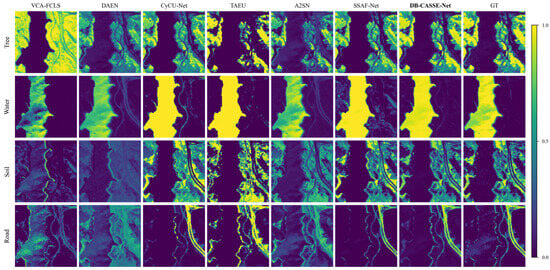
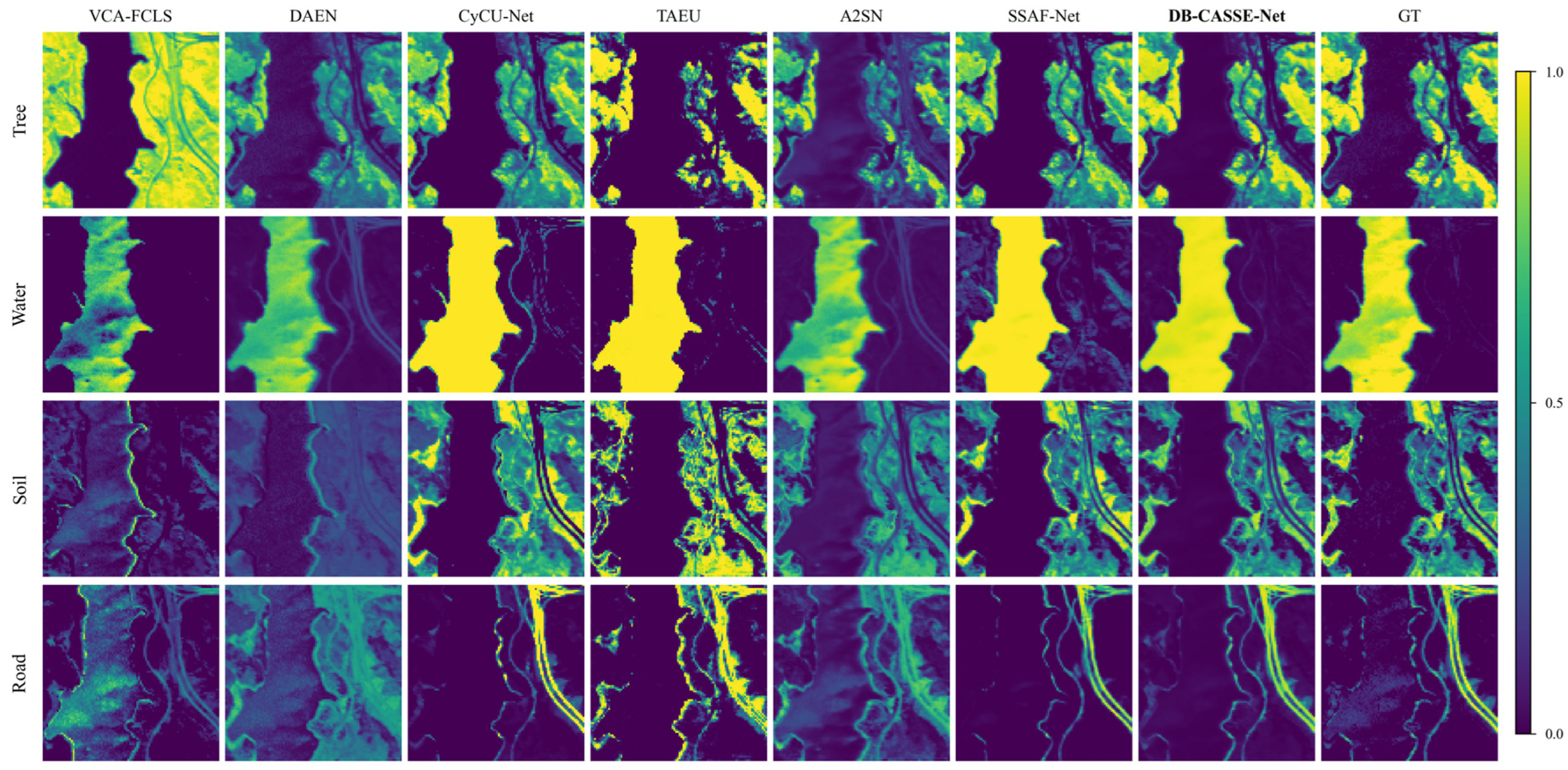
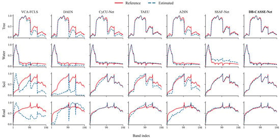
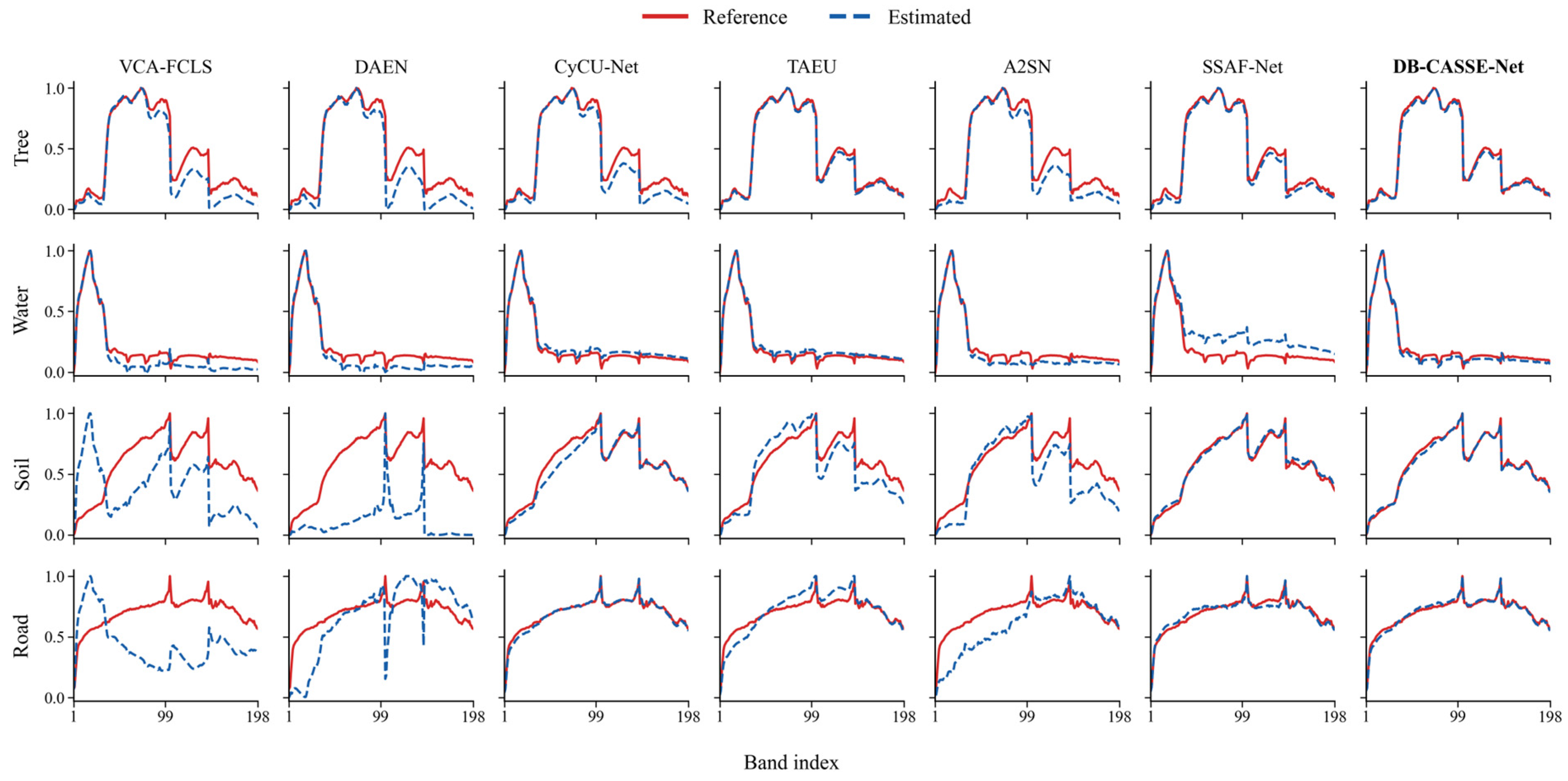
The Jasper Ridge dataset was acquired by the Airborne Visible/Infrared Imaging Spectrometer. The original image contains 512 × 614 pixels and 224 spectral bands spanning 380–2500 nm. A widely used 100 × 100-pixel subregion was analyzed, and bands strongly affected by atmospheric interference and water-vapor absorption were removed, leaving 198 valid bands. The scene contains four endmembers—tree, water, soil, and road—with substantial mixing and complex spatial boundaries. Table 3 and Table 4 report the quantitative results, while Figure 7 and Figure 8 show the abundance maps and endmember spectra, respectively.
Table 3.
Abundance RMSE on the Jasper Ridge dataset. Annotation: bold red text indicates the best results and bold blue text indicates the suboptimal results.
Table 4.
Endmember SAD on the Jasper Ridge dataset. Annotation: bold red text indicates the best results and bold blue text indicates the suboptimal results.
Figure 7.
Abundance maps produced by the compared methods on the Jasper Ridge dataset.
Figure 8.
Estimated endmember spectra on the Jasper Ridge dataset.
Table 3 and Table 4 show that DB-CASSE-Net achieves the lowest mean abundance error and mean spectral angle on Jasper Ridge. Its abundance RMSE is lower than that of every comparison method for all four endmembers. Figure 7 shows that VCA–FCLS substantially overestimates tree and soil and confuses materials. Because VCA identifies endmembers from simplex vertices, insufficient pure pixels or strong mixing propagates endmember errors to the subsequent FCLS abundance solution. DAEN produces smoother maps but exhibits diffusion near road, soil, and water boundaries, indicating that spectral reconstruction alone does not adequately preserve narrow structures. CyCU-Net recovers the main spatial outlines, but parts of the water and road maps are oversaturated or resemble hard segmentation, resulting in errors in continuous abundance variation. TAEU and A2SN improve regional consistency, although TAEU remains fragmented or overestimated in some mixed areas and A2SN shows leakage at road–soil boundaries. SSAF-Net captures the main distributions of tree, soil, and road, but its water map exhibits overly uniform high-abundance responses within the water region and residual responses outside it. DB-CASSE-Net more closely matches the reference maps and better preserves narrow roads and material interfaces.
For endmember estimation, DB-CASSE-Net obtains the lowest SAD for tree and soil, while CyCU-Net is slightly better for road. Figure 8 shows that DB-CASSE-Net follows the overall spectral shapes and principal absorption features of tree, water, and soil. Its estimated road spectrum is also close to the reference, although CyCU-Net obtains a slightly smaller angle for that endmember. Taken together, DB-CASSE-Net provides the best overall result on this dataset.
3.3. Samson Dataset
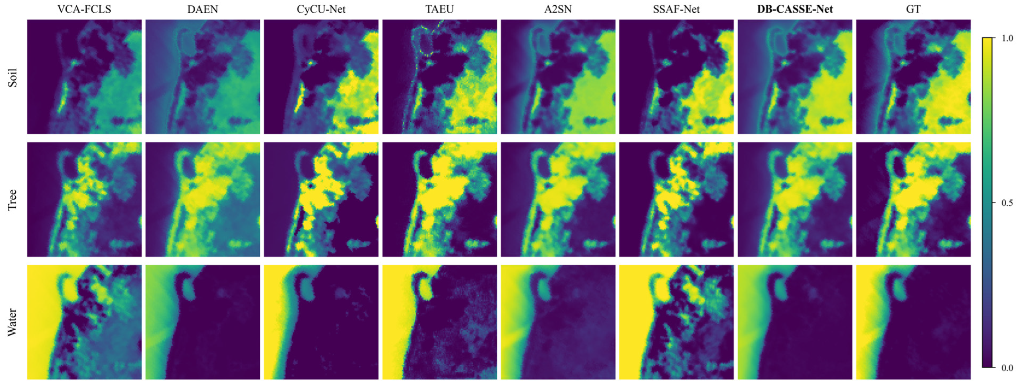
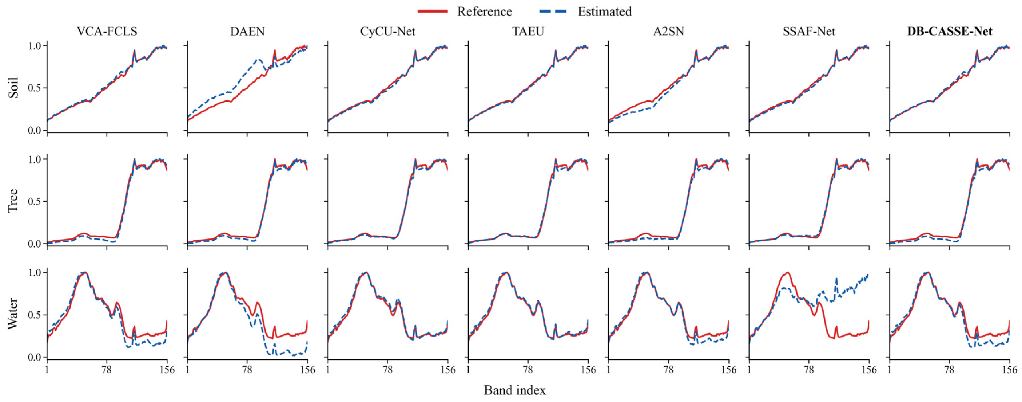
The original Samson HSI contains 952 × 952 pixels and 156 contiguous spectral bands spanning 401–889 nm. To reduce computation and remain consistent with existing unmixing studies, a 95 × 95-pixel subregion was used. It contains three endmembers—soil, tree, and water—and has relatively continuous abundance distributions, allowing methods to be evaluated in both homogeneous regions and material-transition zones. Table 5 and Table 6 present the quantitative results, and Figure 9 and Figure 10 show the abundance maps and estimated endmember spectra, respectively.
Table 5.
Abundance RMSE on the Samson dataset. Annotation: bold red text indicates the best results and bold blue text indicates the suboptimal results.
Table 6.
Endmember SAD on the Samson dataset. Annotation: bold red text indicates the best results and bold blue text indicates the suboptimal results.
Figure 9.
Abundance maps produced by the compared methods on the Samson dataset.
Figure 10.
Estimated endmember spectra on the Samson dataset.
Table 5 indicates that DB-CASSE-Net ranks second in mean abundance error on Samson. It achieves the lowest soil abundance RMSE and the second-lowest water abundance RMSE, while its tree abundance error remains higher than those of A2SN and TAEU. Figure 9 shows that DB-CASSE-Net recovers the main distributions of all three materials and maintains gradual abundance transitions between regions. A2SN provides more accurate tree abundance estimates and achieves the lowest mean abundance error, whereas CyCU-Net performs best for water but exhibits larger errors for soil and tree. SSAF-Net captures the broad material distributions but retains scattered responses outside the principal tree and water regions. Its larger abundance errors, particularly for water, limit its overall abundance estimation accuracy. But compared with these results, DB-CASSE-Net provides competitive estimates across all three materials.
Table 6 and Figure 10 show that DB-CASSE-Net does not achieve the lowest mean endmember SAD on Samson. The estimated soil spectrum follows the reference reasonably well, whereas deviations remain in the tree and water spectra. These results indicate that abundance estimation does not necessarily coincide with the lowest endmember error. Joint optimization of abundances and endmembers under the reconstruction objective may contribute to this difference.
3.4. Urban Dataset
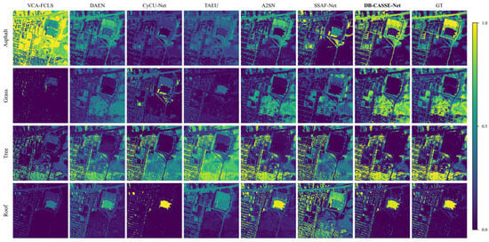
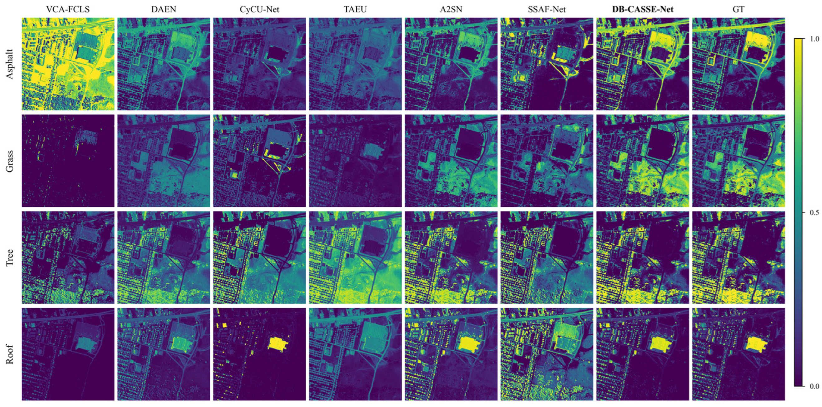
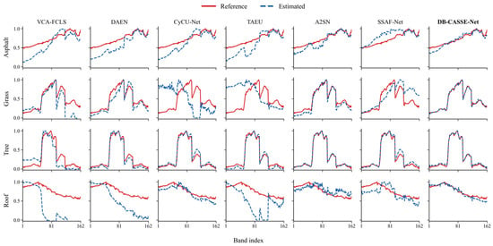
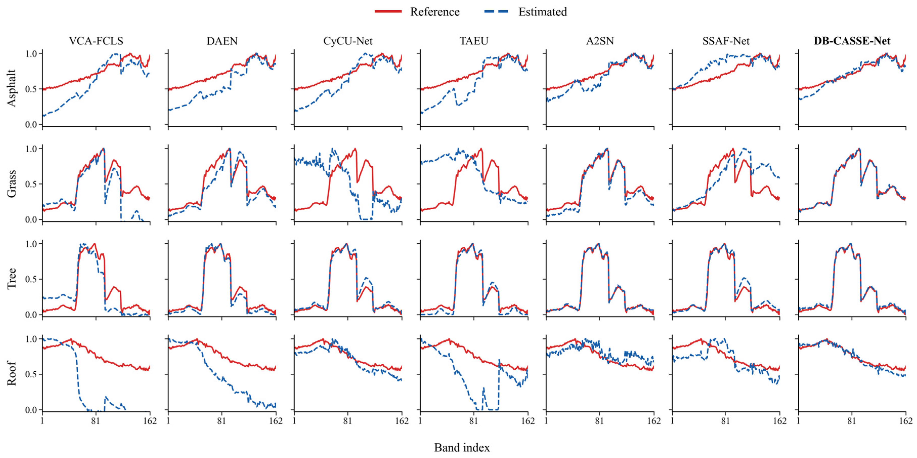
The Urban dataset was acquired by the Hyperspectral Digital Imagery Collection Experiment (HYDICE) sensor. The original image contains 307 × 307 pixels and 210 bands spanning 400–2500 nm. After bands affected by atmospheric interference, water-vapor absorption, and low signal-to-noise ratio were removed, 162 valid bands remained. The scene contains four endmembers—asphalt, grass, tree, and roof—and exhibits fragmented distributions, pronounced interleaving of vegetation and construction materials, and many mixed pixels. It therefore places greater demands on the model’s ability to preserve spatial boundaries. Table 7 and Table 8 report the quantitative results, and Figure 11 and Figure 12 show the abundance maps and endmember spectra, respectively.
Table 7.
Abundance RMSE on the Urban dataset. Annotation: bold red text indicates the best results and bold blue text indicates the suboptimal results.
Table 8.
Endmember SAD on the Urban dataset. Annotation: bold red text indicates the best results and bold blue text indicates the suboptimal results.
Figure 11.
Abundance maps produced by the compared methods on the Urban dataset.
Figure 12.
Estimated endmember spectra on the Urban dataset.
Table 7 and Table 8 show that DB-CASSE-Net obtains both the lowest mean abundance error and the lowest mean spectral angle on Urban. Figure 11 shows that VCA–FCLS markedly overestimates asphalt and fails to recover the grass distribution, illustrating how endmember-extraction errors affect abundance estimation in an urban scene with many mixed pixels and insufficient pure-pixel conditions. DAEN produces overly smooth maps and confuses grass, tree, and construction materials. CyCU-Net and TAEU identify the principal regions, but some maps are excessively discrete or nearly binary and do not capture continuous within-class abundance variation adequately. A2SN performs well overall but still shows cross-region responses near asphalt, vegetation, and roofs. SSAF-Net identifies some road and building structures, but its roof map contains strong responses outside the principal roof regions, consistent with its largest roof abundance error among the evaluated methods. The DB-CASSE-Net maps are more consistent with the reference distributions, localize roof regions clearly, and preserve fragmented structures such as roads, building edges, and vegetation patches.
For endmember estimation, DB-CASSE-Net achieves the smallest SAD for asphalt, grass, and roof, while its tree estimate is slightly less accurate than that of A2SN. Figure 12 shows that the principal shapes and absorption features of the grass and roof spectra are fitted well. Although the asphalt estimate has amplitude deviations in some bands, its overall direction remains consistent with the reference. These results give DB-CASSE-Net the best overall performance on the Urban dataset.
3.5. Module Ablation Study
We conducted a module ablation study on Jasper and Samson to examine the contributions of CAS and the spectral skip connection. Four configurations were compared by enabling or disabling these components, with a standard 3 × 3 convolution replacing CAS when it was disabled. The training settings and prepared initial endmembers were kept unchanged. The relevant results are shown in Table 9.
Table 9.
Module ablation results.
3.6. Computational Cost and Runtime
We further assess the computational requirements of DB-CASSE-Net to complement the unmixing results presented above. Table 10 summarizes the parameter counts and estimated main-operation FLOPs for the three dataset-specific input sizes and sampling configurations. Forward latency was measured on an NVIDIA GeForce RTX 2060 using PyTorch 2.5.1 and CUDA 11.8, with batch size 1 and FP32 inference. The model was evaluated with gradient computation disabled, and the inputs were already resident on the GPU. After 50 warm-up passes, 500 forward passes were timed in five blocks, with 10 additional warm-up passes between blocks. CUDA events recorded individual durations, with synchronization before and after each block. The reported values are the mean and sample standard deviation of all 500 measurements, excluding data loading, preprocessing, CPU–GPU transfer, and optimization. All three configurations contain fewer than 0.38 million parameters. Their parameter counts differ because of the dataset-specific spectral dimensions, endmember numbers, and sampling configurations. Although the Urban configuration has the fewest parameters, its larger spatial extent results in the highest estimated computational cost, at 61.5227 GFLOPs. Correspondingly, Jasper Ridge and Samson have similar mean forward latencies of approximately 3.6 ms, whereas Urban requires 46.08 ms. These measurements characterize the cost of a complete-scene forward pass under the reported hardware and precision settings.
Table 10.
Computational cost and forward-pass efficiency of DB-CASSE-Net.
4. Conclusions
This paper addresses the challenge that conventional convolutional networks struggle to adapt to irregular boundaries, elongated structures, and fragmented regions in hyperspectral images by proposing a dual-branch unmixing network named DB-CASSE-Net. This method employs restricted adaptive sampling to model the local spatial structure; utilizes spectral branches, SE feature re-calibration, and spectral skip connections to enhance material discrimination information; and integrates a linear decoder that satisfies physical constraints to jointly estimate endmembers and their abundances. Experimental results demonstrate that the proposed method effectively balances both the spatial distribution of abundance and the spectral recovery of endmembers. However, several limitations remain: the endmember initialization strategy and sampling configuration of the proposed method still exhibit a certain degree of dataset dependency, which may contribute to the less pronounced advantages observed in scenes with relatively simple spatial structures; additionally, the spectral recovery stability for some endmembers requires further improvement. Therefore, future work should focus on evaluating the robustness of unmixing performance to different initialization methods. Further validation on larger-scale hyperspectral scenes with more complex spatial structures will also be conducted to more comprehensively evaluate the generalization capability of the proposed adaptive spatial sampling strategy.
Author Contributions
Conceptualization, Q.L. and Y.L.; methodology, Q.L. and Y.L.; software, Y.L.; validation, Y.L.; formal analysis, M.L. and J.L.; investigation, Q.L. and M.L.; resources, M.L.; data curation, Y.L. and P.T.; writing—original draft preparation, Y.L.; writing—review and editing, Q.L. and J.L.; visualization, Y.L.; supervision, M.L. and P.T.; project administration, Q.L. and J.L.; funding acquisition, Q.L. All authors have read and agreed to the published version of the manuscript.
Funding
This work was supported in part by National Natural Science Foundation of China (No. 62362041) and the 2023 Ji’an City Enterprise “Open Competition for the Best Candidates” Project (No. 2025zkhx0027).
Data Availability Statement
The Jasper Ridge, Samson, and Urban hyperspectral datasets analyzed in this study are publicly available benchmark datasets. https://github.com/UPCGIT/Hyperspectral-Unmixing-Models/tree/main/Datasets, accessed on 15 November 2026.
Acknowledgments
All authors would sincerely thank the reviewers and editors for their suggestions and opinions for improving this article. During the preparation of this manuscript, the authors used GPT-5.6 for the purposes of auxiliary code design and manuscript refinement. The authors have reviewed and edited the output and take full responsibility for the content of this publication.
Conflicts of Interest
The authors declare no conflicts of interest.
References
- Nagasubramanian, K.; Jones, S.; Singh, A.K.; Sarkar, S.; Singh, A.; Ganapathysubramanian, B. Plant disease identification using explainable 3D deep learning on hyperspectral images. Plant Methods 2019, 15, 98. [Google Scholar] [CrossRef] [Scilit] [PubMed]
- Tong, Q.; Zhang, B.; Zheng, L. Hyperspectral Remote Sensing: Principles, Technologies, and Applications; Higher Education Press: Beijing, China, 2006. [Google Scholar]
- Zhang, B. Advancement of hyperspectral image processing and information extraction. J. Remote Sens. 2016, 20, 1062–1090. [Google Scholar] [CrossRef] [Scilit]
- Keshava, N.; Mustard, J.F. Spectral unmixing. IEEE Signal Process. Mag. 2002, 19, 44–57. [Google Scholar] [CrossRef] [Scilit]
- Bioucas-Dias, J.M.; Plaza, A.; Dobigeon, N.; Parente, M.; Du, Q.; Gader, P.; Chanussot, J. Hyperspectral unmixing overview: Geometrical, statistical, and sparse regression-based approaches. IEEE J. Sel. Top. Appl. Earth Obs. Remote Sens. 2012, 5, 354–379. [Google Scholar] [CrossRef] [Scilit]
- Boardman, J.W.; Kruse, F.A.; Green, R.O. Mapping target signatures via partial unmixing of AVIRIS data. In Summaries of the Fifth JPL Airborne Earth Science Workshop, Volume 1: AVIRIS Workshop; JPL Publication 95-1: Pasadena, CA, USA, 1995; pp. 23–26. [Google Scholar]
- Nascimento, J.M.P.; Bioucas-Dias, J.M. Vertex component analysis: A fast algorithm to unmix hyperspectral data. IEEE Trans. Geosci. Remote Sens. 2005, 43, 898–910. [Google Scholar] [CrossRef] [Scilit]
- Winter, M.E. N-FINDR: An algorithm for fast autonomous spectral end-member determination in hyperspectral data. In Proceedings of the SPIE 3753, Imaging Spectrometry V; SPIE: Bellingham, WA, USA, 1999; pp. 266–275. [Google Scholar] [CrossRef] [Scilit]
- Dobigeon, N.; Moussaoui, S.; Coulon, M.; Tourneret, J.-Y.; Hero, A.O. Joint Bayesian endmember extraction and linear unmixing for hyperspectral imagery. IEEE Trans. Signal Process. 2009, 57, 4355–4368. [Google Scholar] [CrossRef] [Scilit]
- Bioucas-Dias, J.M.; Figueiredo, M.A.T. Alternating direction algorithms for constrained sparse regression: Application to hyperspectral unmixing. In 2010 2nd Workshop on Hyperspectral Image and Signal Processing: Evolution in Remote Sensing; IEEE: New York, NY, USA, 2010; pp. 1–4. [Google Scholar] [CrossRef] [Scilit]
- Lee, D.D.; Seung, H.S. Learning the parts of objects by non-negative matrix factorization. Nature 1999, 401, 788–791. [Google Scholar] [CrossRef] [Scilit] [PubMed]
- Miao, L.; Qi, H. Endmember extraction from highly mixed data using minimum volume constrained nonnegative matrix factorization. IEEE Trans. Geosci. Remote Sens. 2007, 45, 765–777. [Google Scholar] [CrossRef] [Scilit]
- Heylen, R.; Parente, M.; Gader, P. A review of nonlinear hyperspectral unmixing methods. IEEE J. Sel. Top. Appl. Earth Obs. Remote Sens. 2014, 7, 1844–1868. [Google Scholar] [CrossRef] [Scilit]
- Dobigeon, N.; Tourneret, J.-Y.; Richard, C.; Bermudez, J.C.M.; McLaughlin, S.; Hero, A.O. Nonlinear unmixing of hyperspectral images: Models and algorithms. IEEE Signal Process. Mag. 2014, 31, 82–94. [Google Scholar] [CrossRef] [Scilit]
- Su, Y.C.; Xu, R.Q.; Gao, L.R.; Han, Z.; Sun, X. Development of deep-learning-based hyperspectral remote-sensing image unmixing. Natl. Remote Sens. Bull. 2024, 28, 1–19. [Google Scholar] [CrossRef] [Scilit]
- Qin, K.; Hao, Y.; Zhao, Y.; Cui, X.; Yang, Y.; Zhu, L.; Tian, Q. A survey on hyperspectral remote-sensing unmixing techniques based on autoencoders. Infrared Laser Eng. 2025, 54, 20250131. [Google Scholar] [CrossRef] [Scilit]
- Li, X.; Ding, M.; Pižurica, A. Group convolutional neural networks for hyperspectral image classification. In Proceedings of the 2019 IEEE International Conference on Image Processing (ICIP), Taipei, Taiwan, 22–25 September 2019; IEEE: New York, NY, USA, 2019; pp. 639–643. [Google Scholar] [CrossRef] [Scilit]
- Li, X.; Gu, Y.; Xu, L.; Pižurica, A. An enhanced geometric-spectral feature learning framework for airborne multispectral point cloud classification. IEEE Trans. Geosci. Remote Sens. 2026. [Google Scholar] [CrossRef] [Scilit]
- Wang, D.; Gao, L.; Qu, Y.; Sun, X.; Liao, W. Frequency-to-spectrum mapping GAN for semisupervised hyperspectral anomaly detection. CAAI Trans. Intell. Technol. 2023, 8, 1258–1273. [Google Scholar] [CrossRef] [Scilit]
- Wang, D.; Zhuang, L.; Gao, L.; Sun, X.; Huang, M.; Plaza, A. PDBSNet: Pixel-Shuffle Downsampling Blind-Spot Reconstruction Network for Hyperspectral Anomaly Detection. IEEE Trans. Geosci. Remote Sens. 2023, 61, 5511914. [Google Scholar] [CrossRef] [Scilit]
- Zhang, X.; Sun, Y.; Zhang, J.; Wu, P.; Jiao, L. Hyperspectral unmixing via deep convolutional neural networks. IEEE Geosci. Remote Sens. Lett. 2018, 15, 1755–1759. [Google Scholar] [CrossRef] [Scilit]
- Ren, L.; Han, Z.; Gao, L.; Zhang, T.; Wu, R.; Zhang, H. Advances in hyperspectral image unmixing: From algorithmic frameworks to practical applications. Inf. Geogr. 2026, 2, 100035. [Google Scholar] [CrossRef] [Scilit]
- Palsson, B.; Sigurdsson, J.; Sveinsson, J.R.; Ulfarsson, M.O. Hyperspectral unmixing using a neural network autoencoder. IEEE Access 2018, 6, 25646–25656. [Google Scholar] [CrossRef] [Scilit]
- Ozkan, S.; Kaya, B.; Akar, G.B. EndNet: Sparse autoencoder network for endmember extraction and hyperspectral unmixing. IEEE Trans. Geosci. Remote Sens. 2019, 57, 482–496. [Google Scholar] [CrossRef] [Scilit]
- Qu, Y.; Qi, H. uDAS: An untied denoising autoencoder with sparsity for spectral unmixing. IEEE Trans. Geosci. Remote Sens. 2019, 57, 1698–1712. [Google Scholar] [CrossRef] [Scilit]
- Palsson, B.; Ulfarsson, M.O.; Sveinsson, J.R. Convolutional autoencoder for spectral-spatial hyperspectral unmixing. IEEE Trans. Geosci. Remote Sens. 2021, 59, 535–549. [Google Scholar] [CrossRef] [Scilit]
- Hua, Z.; Li, X.; Jiang, J.; Zhao, L. Gated autoencoder network for spectral-spatial hyperspectral unmixing. Remote Sens. 2021, 13, 3147. [Google Scholar] [CrossRef] [Scilit]
- Xu, X.; Song, X.; Li, T.; Shi, Z.; Pan, B. Deep autoencoder for hyperspectral unmixing via global-local smoothing. IEEE Trans. Geosci. Remote Sens. 2022, 60, 1–16. [Google Scholar] [CrossRef] [Scilit]
- Jin, Q.; Ma, Y.; Fan, F.; Huang, J.; Mei, X.; Ma, J. Adversarial Autoencoder Network for Hyperspectral Unmixing. IEEE Trans. Neural Netw. Learn. Syst. 2023, 34, 4555–4569. [Google Scholar] [CrossRef] [Scilit] [PubMed]
- Guo, Z.; Xiao, M.; Zhu, F.; Chen, X.; Shankar, A.; Zamani, M.; Singh, S.K. A manifold-based adversarial autoencoder with Fourier convolution for hyperspectral unmixing. Appl. Soft Comput. 2025, 177, 113176. [Google Scholar] [CrossRef] [Scilit]
- Xu, M.; Xu, J.; Liu, S.; Sheng, H.; Yang, Z. Multiscale Convolutional Mask Network for Hyperspectral Unmixing. IEEE J. Sel. Top. Appl. Earth Obs. Remote Sens. 2024, 17, 3687–3700. [Google Scholar] [CrossRef] [Scilit]
- Ghosh, P.; Roy, S.K.; Koirala, B.; Rasti, B.; Scheunders, P. Hyperspectral unmixing using transformer network. IEEE Trans. Geosci. Remote Sens. 2022, 60, 5535116. [Google Scholar] [CrossRef] [Scilit]
- Yang, Z.; Xu, M.; Liu, S.; Sheng, H.; Wan, J. UST-Net: A U-shaped transformer network using shifted windows for hyperspectral unmixing. IEEE Trans. Geosci. Remote Sens. 2023, 61, 1–15. [Google Scholar] [CrossRef] [Scilit]
- Tao, X.; Paoletti, M.E.; Wu, Z.; Haut, J.M.; Ren, P.; Plaza, A. An abundance-guided attention network for hyperspectral unmixing. IEEE Trans. Geosci. Remote Sens. 2024, 62, 5505414. [Google Scholar] [CrossRef] [Scilit]
- Han, Z.; Hong, D.; Gao, L.; Yao, J.; Zhang, B.; Chanussot, J. Multimodal hyperspectral unmixing: Insights from attention networks. IEEE Trans. Geosci. Remote Sens. 2022, 60, 5524913. [Google Scholar] [CrossRef] [Scilit]
- Tao, X.; Koirala, B.; Rasti, B.; Plaza, A.; Scheunders, P. A spectral-spatial attention network for hyperspectral unmixing. IEEE Trans. Geosci. Remote Sens. 2025, 63, 5516315. [Google Scholar] [CrossRef] [Scilit]
- Gao, W.; Yang, J.; Zhang, Y.; Akoudad, Y.; Chen, J. SSAF-Net: A spatial-spectral adaptive fusion network for hyperspectral unmixing with endmember variability. IEEE Trans. Geosci. Remote Sens. 2025, 63, 5506015. [Google Scholar] [CrossRef] [Scilit]
- Cui, X.; Zhang, X.; Dai, A.; Sun, D. SSTNT: A spatial–spectral similarity guided Transformer-in-Transformer for hyperspectral unmixing. Photonics 2026, 13, 276. [Google Scholar] [CrossRef] [Scilit]
- Cao, H.; Meng, F.; Sun, H.; Cui, X.; Shao, D. A theory-guided Transformer for interpretable hyperspectral unmixing. Remote Sens. 2026, 18, 886. [Google Scholar] [CrossRef] [Scilit]
- Dai, J.; Qi, H.; Xiong, Y.; Li, Y.; Zhang, G.; Hu, H.; Wei, Y. Deformable convolutional networks. In Proceedings of the IEEE International Conference on Computer Vision; IEEE: New York, NY, USA, 2017; pp. 764–773. [Google Scholar] [CrossRef] [Scilit]
- Zhang, X.; Song, Y.; Song, T.; Yang, D.; Ye, Y.; Zhou, J.; Zhang, L. AKConv: Convolutional kernel with arbitrary sampled shapes and arbitrary number of parameters. arXiv 2023, arXiv:2311.11587v1. [Google Scholar] [CrossRef] [Scilit]
- Qu, K.; Wang, H.; Ding, M.; Luo, X.; Bao, W. DGMNet: Hyperspectral unmixing dual-branch network integrating adaptive hop-aware GCN and neighborhood offset Mamba. Remote Sens. 2025, 17, 2517. [Google Scholar] [CrossRef] [Scilit]
- Hu, J.; Shen, L.; Sun, G. Squeeze-and-excitation networks. In Proceedings of the IEEE Conference on Computer Vision and Pattern Recognition; IEEE: New York, NY, USA, 2018; pp. 7132–7141. [Google Scholar] [CrossRef] [Scilit]
- Heinz, D.C.; Chang, C.-I. Fully constrained least squares linear spectral mixture analysis method for material quantification in hyperspectral imagery. IEEE Trans. Geosci. Remote Sens. 2001, 39, 529–545. [Google Scholar] [CrossRef] [Scilit]
- Su, Y.; Li, J.; Plaza, A.; Marinoni, A.; Gamba, P.; Chakravortty, S. DAEN: Deep autoencoder networks for hyperspectral unmixing. IEEE Trans. Geosci. Remote Sens. 2019, 57, 4309–4321. [Google Scholar] [CrossRef] [Scilit]
- Gao, L.; Han, Z.; Hong, D.; Zhang, B.; Chanussot, J. CyCU-Net: Cycle-consistency unmixing network by learning cascaded autoencoders. IEEE Trans. Geosci. Remote Sens. 2022, 60, 5503914. [Google Scholar] [CrossRef] [Scilit]

Disclaimer/Publisher’s Note: The statements, opinions and data contained in all publications are solely those of the individual author(s) and contributor(s) and not of MDPI and/or the editor(s). MDPI and/or the editor(s) disclaim responsibility for any injury to people or property resulting from any ideas, methods, instructions or products referred to in the content. |
© 2026 by the authors. Licensee MDPI, Basel, Switzerland. This article is an open access article distributed under the terms and conditions of the Creative Commons Attribution (CC BY) license.