


Highlights
What are the main findings?
- Among eight evaluated algorithms, HYB2 and MR4B showed the strongest held-out validation performance.
- Bootstrap resampling indicated comparatively low variability in validation R2 for HYB2 and MR4B, while leave-one-region-out cross-validation (LORO-CV) revealed limited geographic transferability.
What are the implications of the main findings?
- Multiple performance metrics and regional cross-validation are required before an empirical aDOM algorithm is considered for operational use.
- Regionally adaptive or optical-water-type-based approaches may improve transferability when supported by broader, independently validated datasets.
Abstract
Accurate retrieval of dissolved organic matter absorption at 440 nm (aDOM(440)) remains challenging in optically complex coastal waters. This study evaluated eight empirical algorithms using 203 paired observations of in situ aDOM(440) and remote-sensing reflectance from four marine regions surrounding Korea. Five formulations were recalibrated using Huber regression with a log10-transformed response, while three established algorithms retained published coefficients. The dataset comprised 162 calibration and 41 held-out validation observations. HYB1 achieved the highest calibration R2 (0.416), whereas HYB2 performed best in validation (R2 = 0.500; RMSE = 0.0198 m−1), followed by MR4B (R2 = 0.486; RMSE = 0.0200 m−1). Bootstrap resampling of fixed validation predictions indicated comparatively lower variability in R2 for HYB2 and MR4B, with overlapping confidence intervals. Leave-one-region-out cross-validation highlighted limited geographic transferability, particularly for HYB2 and MR4B in the West Sea. Applying the algorithm to Geostationary Ocean Color Imager-II (GOCI-II) imagery revealed algorithm-dependent retrieval magnitudes and spatial patterns; accuracy assessment requires concurrent field observations. These findings identify HYB2 and MR4B as promising candidates for regional refinement and provide a foundation for advancing GOCI-II-based monitoring of coastal aDOM(440).
1. Introduction
Colored dissolved organic matter (CDOM) is the light-absorbing part of dissolved organic matter that plays a crucial role in tracking carbon dynamics in coastal waters. In optical remote sensing studies, CDOM is quantitatively parameterized by its absorption coefficient at a specific wavelength, hereafter referred to as absorption coefficient of dissolved organic matter (aDOM). Because aDOM increases exponentially toward ultraviolet and blue wavelengths, it accounts for a substantial fraction (approximately 20–70%) of total absorption near 443 nm in coastal systems [1,2]. This spectral behavior supports the use of ocean-color remote sensing to examine coastal gradients and the spatial distribution of dissolved organic matter associated with riverine inputs and marine processes. Compared with discrete ship-based sampling, satellite observations provide broader spatial coverage and more frequent monitoring of these patterns.
Approaches for retrieving aDOM are commonly divided into semi-analytical inherent-optical-property inversions and empirical band-ratio algorithms. Semi-analytical frameworks, including the quasi-analytical algorithm and generalized IOP models, partition total absorption into constituent components, but separating aDOM from non-algal-particle absorption remains difficult in optically complex waters [1,2]. Empirical blue–green band-ratio algorithms are therefore widely used for coastal aDOM retrieval [3,4]. Their coefficients, however, may not transfer consistently among optical environments and regions [2], and short-wavelength atmospheric-correction residuals can further increase uncertainty [5]. This study examines whether a maximum-band-ratio structure, adapted from OC-family chlorophyll algorithms, can reduce dependence on any single blue band. The approach compares several blue-to-green ratios, selects the maximum, and relates it to aDOM through polynomial regression [6].
The Geostationary Ocean Color Imager-II (GOCI-II) observes its local coverage area up to 10 times per day at hourly intervals. The sensor provides 12 ocean-color bands from 380 to 865 nm at 250 m spatial resolution, together with a wide navigation band [5,7]. Its operational aDOM(440) product uses a regional adaptation of the Yellow Sea Large Marine Ecosystem Ocean Color algorithm, which was developed for the Yellow and East China Seas (southwest of the Korean Peninsula) and uses reflectance ratios at 443, 490, and 555 nm [8,9]. The algorithm theoretical basis document reports mean percentage differences of approximately 40% [9].
The accuracy of empirical aDOM retrieval depends on the spectral characteristics of all optically active water constituents. In coastal waters, phytoplankton absorption, aDOM and non-algal particle (NAP) absorption can overlap spectrally, making it difficult to attribute changes in blue–green remote-sensing reflectance (Rrs.) exclusively to aDOM [1,2,10]. In particular, variations in chlorophyll-a concentration, phytoplankton pigment composition, and cell size can modify blue-band absorption, potentially affecting the band ratios used in empirical aDOM algorithms [11]. In addition, suspended particulate matter (SPM), including non-algal particles, can alter both absorption and backscattering, thereby modifying the magnitude and spectral shape of Rrs. These effects are particularly relevant in optically complex coastal waters, where the relative contributions of dissolved and particulate constituents can vary substantially [2,10]. Consequently, blue–green band-ratio algorithms cannot fully isolate the aDOM signal from phytoplankton and particle-related optical variability, which may introduce additional uncertainty into aDOM(440) retrievals.
Since the global algorithms might not transfer reliably to the coastal waters of Korea and the operational GOCI-II product is still uncertain, the present study has developed and evaluated empirical formulae for retrieving aDOM(440). The operational YOC algorithm was compared with adapted versions of the older models as well as with new hybrid and multi-band formulations. The performance of the algorithms was evaluated using randomly 80:20 calibration–validation split, fixed-prediction bootstrap resampling, and leave-one-region-out cross-validation (LORO-CV) to examine sampling variability and geographic transferability. The algorithms were also applied to the GOCI-II imagery in order to compare the spatial plume patterns and to check the consistency of the hourly retrievals throughout the day.
2. Materials and Methods
The research involved taking paired in situ measurements of Rrs and aDOM(440) in the coastal waters of South Korea from April 2022 through to August 2024. The in situ dataset included station identifiers, latitude, longitude, cruise identifiers, and sampling time (date and local time). In total, 374 samples were collected from diverse marine environments, including the East Sea (N = 79), South Sea (N = 91), West Sea (N = 181), and East China Sea (N = 23; sampling area southwest of Jeju Island). Through a standard ocean color (OC) quality control (QC) process, 203 samples were finally selected for analysis (Figure 1). These in situ observations were conducted and maintained by the Korea Ocean Satellite Center (KOSC) at the Korea Institute of Ocean Science and Technology (KIOST).
Figure 1.
Study area around the Korean Peninsula showing the distribution of 203 final quality-controlled in situ aDOM observation stations across the South Sea, West Sea, East Sea, and East China Sea.
The in situ dataset included station identifiers, geographic coordinates, sampling areas, and measurement dates and local times. As standardized cruise identifiers were not consistently available, sampling-date groups were used to summarize the temporal distribution of the observations (Table 1).
Table 1.
Distribution of in situ aDOM(440) samples by region, season, and sampling-date group. Values are reported separately for the calibration and validation subsets. The aDOM(440) range is the minimum–maximum observed value in each category, rounded to three decimal places.
2.1. In Situ Data
2.1.1. In Situ Observations for Rrs
Above-water hyperspectral radiometric measurements were conducted using a three-channel TriOS RAMSES system (TriOS Mess- und Datentechnik GmbH, Rastede, Germany). An Advanced Cosine Collector for visible wavelengths (ACC-VIS) irradiance sensor with a cosine collector measured downwelling plane irradiance, Ed(0+, λ), while two Advanced Radiance Collector for visible wavelengths (ARC-VIS) sensors with a 7° field of view measured the sea-viewing total radiance, Lt (λ), and sky radiance, Lsky (λ). Here, Lt (λ) represents the sea-viewing signal before surface-reflection correction and includes both water-leaving radiance and sky radiance reflected at the air–water interface. The irradiance sensor was mounted horizontally in an unobstructed position. The sea- and sky-viewing sensors were oriented at 40° from nadir and zenith, respectively, with a relative azimuth of approximately 135° to the solar azimuth to minimize direct sun glint and vessel shadowing [12,13].
The radiometers were powered on at least 30 min before measurement to ensure thermal stability. Ed, Lt, and Lsky were recorded as simultaneously as the acquisition system permitted. At each station, spectra were acquired for approximately 3 min to capture the short-term variability caused by surface waves and ambient illumination, with three consecutive spectra of each quantity recorded every 20 s. Raw digital counts were converted to calibrated spectral radiance and irradiance using a sensor-specific device and radiometric calibration files. Dynamic dark-current correction, radiometric sensitivity scaling, and wavelength calibration produced calibrated spectra over approximately 320–950 nm. Spectra affected by vessel motion, hull contamination, foam, whitecaps, strong sun glint, transient cloud passages, or sensor shading were excluded [13,14,15].
Rrs was derived by removing the surface-reflected sky-radiance component from the sea-viewing signal. The measured total radiance was expressed as the sum of water-leaving radiance, Lw (λ), and surface-reflected sky radiance, Lr (λ):
where Ed(λ) is the above-surface downwelling plane irradiance and the reflected component is parameterized using an effective surface-reflectance factor, ρ:
Rrs(λ) = Lw(λ) ∕ Eⅆ(λ) = [Lt(λ) − Lr(λ)] ∕ Ed(λ) [sr−1]
Lr(λ) = ρ ⋅ Lsky(λ)
Following the two-stage correction of Moon et al. [16], the initial correction for the prescribed 40° viewing geometry under relatively calm conditions (wind speed ≤ 5 m s−1) used a baseline surface-reflectance factor of 0.025:
where Rrs,init(λ) is the initially corrected remote-sensing reflectance obtained after subtracting the surface-reflected sky-radiance component estimated using the baseline reflectance factor of 0.025.
Rrs,init(λ) = [Lt(λ) − 0.025 ⋅ Lsky(λ)] ∕ Ed(λ)
Because roughness at the air-water interface can leave residual reflected radiance after the initial correction, the residual factor, Δρ, was estimated by spectral fitting over 770–900 nm using the near-infrared (NIR) bio-optical model implemented in the KOSC processing procedure. The final spectrum was then calculated as:
Rrs(λ) = Rrs,init(λ) − [Δρ ⋅ Lsky(λ)] ∕ Ed(λ)
Only spectra meeting all of the QC criteria of Moon et al. [16] were retained: (1) the RMS difference between measured and modeled spectra was < 0.1; (2) the surface-reflection contribution satisfied Rsfc/Rrs < 0.5; (3) estimated NIR absorption satisfied aNIR/[ap(440) + ag(440)] < 0.7; (4) the path-amplification parameter satisfied 0.5 < k < 2; and (5) the spectral-slope parameter satisfied 0 < n < 4. Here, Rsfc = Lr/Ed is the apparent reflectance contribution from surface-reflected sky radiance; aNIR is the residual NIR absorption estimated during spectral fitting; and ap(440) and ag(440) are the particulate and DOM absorption coefficients at 440 nm, respectively. Spectra failing any criterion were rejected, and the retained observations represented station-level Rrs(λ) [13,16].
2.1.2. In Situ aDOM(λ) Measurements
aDOM(λ) was determined from discrete seawater samples using double-beam ultraviolet–visible (UV–Vis) spectrophotometry. Filtration through a nominal 0.2 µm membrane operationally defined the dissolved fraction, whereas the optical measurement quantified the chromophoric fraction of the filtrate [17,18,19].
Water samples from each station were passed through a 25 mm membrane filter with a 0.2 µm pore size using a 50 mL syringe. The syringe was first rinsed three times with approximately 15 mL of the corresponding sample water. The filtered water was transferred into clean, 50 mL amber glass bottles. Prior to sampling, the bottles were immersed in 10% HCl for 24 h, rinsed thoroughly with deionized water, and dried at 100 °C for 1 h. Once cooled, they were capped and stored until use. Each bottle was rinsed with approximately 5 mL of filtrate, which was discarded, and then filled with approximately 45 mL of the remaining filtered sample. The bottles were sealed and stored at 4 °C in the dark until analysis [18,20].
Absorbance spectra were obtained with a CARY-300 double-beam spectrophotometer (Agilent Technologies, Santa Clara, CA, USA) equipped with a 100 mm path length. The instrument was allowed to warm up for a minimum of 1 h before measurements were taken, allowing the baseline and instrument response to stabilize. The optical cells were acid-cleaned, thoroughly rinsed, and conditioned in Milli-Q (Merck KGaA, Darmstadt, Germany) water before use. For baseline correction, the reference and sample cells were filled with bubble-free Milli-Q water and scanned over 250–900 nm. The sample cell was then rinsed, filled with the field sample, capped, and carefully cleaned to remove moisture or particles from the optical windows. Sample absorbance, expressed as optical density (ODs(λ)), was measured over 250–900 nm, with the corresponding Milli-Q baseline denoted as ODb(λ) [18,20].
Before calculating aDOM(λ), the residual long-wavelength signal was inspected over 650–700 nm. Under the KOSC procedure, ODnull was normally calculated as the mean baseline-corrected absorbance over 650–680 nm. Spectra affected by bubbles, residual particles, contaminated optical windows, or a large or sloping long-wavelength offset were reloaded, cleaned, re-filtered, remeasured, or rejected before null correction. When localized spectral noise was present, the averaging interval could be slightly adjusted within the inspected long-wavelength region only when a spectrally flat interval remained. This treatment was consistent with International Ocean Color Coordinating Group (IOCCG) guidance recommending that null correction be restricted to a small, spectrally neutral residual offset [18].
The corrected absorbance was calculated as:
Acorr (λ) = ODs(λ) − ODb(λ) − ODnull
Because spectrophotometric absorbance is expressed on a base-10 logarithmic scale whereas the absorption coefficient is defined using natural-exponential attenuation, aDOM(λ) was calculated as:
where L is the optical path length (L = 0.10 m for the 100 mm cell). For this cell configuration, aDOM(λ) = 23.026 · Acorr(λ). Because the path length was expressed directly in meters, no additional unit-conversion factor was required. The resulting absorption spectra were reported in m−1. The value at 440 nm was extracted directly from the corrected aDOM(λ) spectrum and used as the in situ reference variable throughout this study, which was consistent with the wavelength of the corresponding GOCI-II aDOM(440) product.
aDOM(λ) = ln(10) ⋅ Acorr (λ) ∕ L≈2.303 ⋅ Acorr (λ) ∕ L [m−1]
2.2. GOCI-II Data
GOCI-II, a second-generation geostationary ocean-color sensor aboard GEO-KOMPSAT-2B (GK-2B), was launched in February 2020. It provides up to 10 hourly observations per day (23:16–08:16 UTC) in 12 ocean-color bands spanning 380–865 nm at 250 m resolution over a 2500 km × 2500 km local area centered on the Korean Peninsula. These capabilities support high-frequency monitoring of Northeast Asian coastal waters, although atmospheric correction remains challenging in turbid and high-aerosol conditions [7].
GOCI-II Level-2 Rrs is produced with the standard atmospheric-correction algorithm, which accounts for gaseous absorption, Rayleigh scattering, aerosols, sun glint, whitecaps, bidirectional-reflectance effects, and non-negligible near-infrared water reflectance in turbid coastal waters [5,7]. Product accuracy and long-term consistency also depend on sensor radiometric stability because calibration uncertainty can propagate from top-of-atmosphere radiance into Rrs and subsequent ocean-color products [21].
This study utilized GOCI-II Level-2 ocean color radiometry (OCR) products, comprising atmospherically corrected Rrs at 412, 443, 490, and 555 nm, the operational aDOM(440) product and associated pixel-level QC flags. The operational aDOM(440) product was calculated using a regionally modified YOC formulation tuned for the Yellow and East China Seas [8,9].
For the satellite in situ diagnostic comparison, GOCI-II Level-2 scenes were associated with the 41 held-out validation observations using their sampling dates, times, and geographic coordinates. Satellite Rrs values at 412, 443, 490, and 555 nm were examined at the nearest geolocated pixel to each sampling station. Of the 41 observations, 27 had complete positive Rrs values at all four required wavelengths and were retained for the sample-wise diagnostic comparison. The remaining 14 matchups contained Level-2 fill values (−999) at all four wavelengths. Original Level-2 quality flags were examined to identify the processing conditions associated with these unavailable retrievals, with detailed matchup screening results provided in Supplementary Table S1. Because multiple quality flags can occur simultaneously, they were not interpreted as mutually exclusive physical causes of missing data.
For the spatial and diurnal satellite application, scenes corresponding to available in situ observations were initially considered. However, incomplete valid reflectance coverage, particularly in some coastal areas, limited the visualization of continuous spatial patterns. Therefore, ten hourly GOCI-II Level-2 scenes acquired on 28 July 2025 (08:15–17:15 KST) were selected as the demonstration case. Scene selection considered the availability of hourly observations and predefined quality criteria, including cloud cover below 20%, a sun-glint angle below 25°, low aerosol optical depth, and more than 80% valid coastal pixels. Pixel-level quality flags were also used to screen unreliable retrievals. The selected scenes were used to compare the spatial distributions and hourly behavior of the evaluated algorithms. As no concurrent in situ measurements were available, this application was intended to illustrate algorithm behavior rather than independently validate retrieval accuracy.
2.3. Methodology
The study workflow comprised four sequential steps: (1) preparation and QC of a paired in situ Rrs and aDOM(440) dataset, followed by partitioning into calibration and validation subsets; (2) implementation of existing and newly developed algorithms, including coefficient fitting and wavelength harmonization where required; (3) algorithm validation, cross-validation, and comparative performance assessment; and (4) the application of selected algorithms to GOCI-II imagery for spatial and diurnal evaluation (Figure 2).
Figure 2.
Workflow for the data preparation, algorithm implementation, performance assessment, and GOCI-II application of eight empirical aDOM(440) retrieval algorithms.
2.3.1. In Situ Data Pre-Processing
In situ measurements of aDOM(440) were paired with co-located in situ Rrs at 412, 443, 490, and 555 nm to form a reference dataset. This process followed standard OC QC practices for satellite validation [22]. As a basic physical and technical QC step, all records with negative aDOM(440), non-positive or missing Rrs values at the required wavelengths or incomplete spectral inputs were removed before predictor construction, resulting in a cleaned in situ dataset of N = 203 pairs distributed across the four study regions shown in Figure 1. The cleaned dataset was randomly partitioned into calibration (80%, N = 162) and validation (20%, N = 41) subsets for algorithm development and performance evaluation. Satellite-derived Rrs was not used during this stage.
The in situ Rrs values at the four GOCI-II wavelengths were obtained from a source dataset preprocessed using the corresponding GOCI-II spectral response functions (SRFs). Hyperspectral Rrs spectra were converted to band-equivalent values following the SRF-weighting approach described by Moon et al. [16]:
where (i) denotes a GOCI-II band, λ is wavelength, and SRFi(λ) is the spectral response function of band (i). These preprocessed band-equivalent values were used directly for pairing with in situ aDOM(440) and subsequent algorithm calibration and validation.
Predictor variables were constructed from the in situ Rrs by calculating blue-to-green band reflectance ratios Rrs(412)/Rrs(555), Rrs(443)/Rrs(555), and Rrs(490)/Rrs(555) together with their polynomial terms. These band ratios emphasize spectral contrasts relevant to aDOM variability [4,6]. For the five locally recalibrated formulations, log10[aDOM(440)] was used as the response variable, while individual predictors were constructed using log10 or natural logarithms (ln), as defined in Table 2. The fitted predictions were back-transformed to the original aDOM(440) scale using 10^ŷ without additional bias correction. The three reference algorithms retained their original mathematical formulations.
Table 2.
Predictor definitions and complete prediction equations for the eight algorithms.
Table 3.
Refitted coefficients for the five locally calibrated algorithms.
2.3.2. Algorithm Development
- 1. Operational and Existing aDOM algorithm
Three empirical algorithms were used as benchmarks: the operational GOCI-II algorithm (G2C), the Mannino et al. [4] model (MAN), and the Shanmugam [23] model (SHA) (Table 2). Their original published coefficients were retained without recalibration to test their performance under the regional optical conditions around the Korean Peninsula.
- •
- G2C: The operational GOCI-II aDOM(440) algorithm is a regional adaptation of the YOC formulation developed by Siswanto et al. [8]. It uses a blue-to-green reflectance ratio based on the 443, 490, and 555 nm bands with published operational coefficients (Table 2, Equation 8; [9]).
- •
- MAN and SHA: Both published formulations were evaluated using the available GOCI-II reflectance bands without recalibrating their coefficients. MAN estimates aDOM at 443 nm, whereas the SHA formulation follows Equation (18) in Shanmugam [23], which uses Rrs(443)/Rrs(555) to estimate absorption at 412 nm. Here, 412 nm denotes the absorption output wavelength rather than a reflectance predictor wavelength. No input-band substitution was applied to SHA. Their outputs were subsequently harmonized to 440 nm using the calibration-derived reference spectral slope (Sref), as described in Equations (16)–(19). MAN was originally calibrated for coastal and shelf waters off the northeastern United States using SeaWiFS and MODIS-Aqua data. In contrast, SHA was developed as a broader aDOM retrieval model and evaluated using datasets from different marine environments.
Because SHA and MAN were originally formulated to estimate aDOM at 412 and 443 nm, respectively, their outputs were spectrally harmonized to 440 nm prior to inter-comparison using the standard exponential spectral model for aDOM [10]:
where S is the aDOM spectral slope parameter and λ0 is the reference wavelength. The conversion between two target wavelengths, λ1 and λ2 is defined as [24]:
aDOM(λ) = aDOM(λ0)exp[−S(λ − λ0)]
aDOM(λ2) = aDOM(λ1)exp[−S(λ2 − λ1)]
This approach was consistent with previous studies that converted aDOM between 412 and 440 nm using assumed or measured spectral slopes [24,25]. Accordingly, the MAN and SHA outputs were converted to 440 nm as follows:
aDOM(440) = aDOM(λorig)exp[−Sref(440 − λorig)]
To avoid using independent-validation observations in the estimation of the harmonization parameter, the reference spectral slope (Sref) was derived exclusively from the calibration subset (N = 162). Calibration observations were matched to their measured aDOM spectra using sampling date, station identifier, and geographic coordinates, with sampling time used to resolve duplicate matches. For spectral-slope quality control, aDOM values at 412, 440, and 443 nm were required to exceed 0.002 m−1. Observations failing these criteria or the source-matching checks were excluded from slope estimation.
For each calibration observation, the spectral slope between 412 and 440 nm was calculated as follows:
S(412−440) = ln [aDOM(412)/aDOM(440)]/(440 − 412)
Of the 162 calibration observations, 158 (97.5%) passed the spectral-slope quality-control criteria and were used to estimate Sref. The resulting mean slope was 0.01991 nm−1, with a standard deviation (SD) of 0.00689 nm−1. To evaluate the sensitivity of wavelength harmonization to the assumed spectral slope, three calibration-derived values were considered: the first quartile (Q1 = 0.01631 nm−1), the mean (0.01991 nm−1), and the third quartile (Q3 = 0.02128 nm−1). The calibration-only mean was used as the primary Sref, while Q1 and Q3 were retained as sensitivity scenarios. Independent-validation observations were not used to estimate or select Sref.
The MAN output was harmonized from 443 to 440 nm using the factor exp(3 × Sref), while the SHA output was harmonized from 412 to 440 nm using the factor exp(−28 × Sref). A single pooled Sref was retained because the uneven regional sampling limited the reliability of region-specific slope estimates. For each sensitivity scenario, the MAN and SHA outputs were harmonized to 440 nm using unchanged algorithm coefficients and evaluated against the same independent-validation subset (N = 41). The resulting R2 and RMSE values are provided in Supplementary Table S2.
- 2. Proposed New and Hybrid Algorithms
Five new empirical formulations were developed by modifying and combining predictor structures from existing algorithms. The selected predictors and complete equations are defined in Table 2, and all coefficients in Table 3 were estimated using the calibration dataset.
- •
- Modified YOC (YOC-R): Inspired by the YOC approach of Siswanto et al. [8], YOC-R (Equation 11) combines the specified reflectance ratios in their original and log10-transformed forms, with all coefficients re-estimated using the calibration dataset.
- •
- Hybrid formulations (HYB1 and HYB2): These combine polynomial log-ratio terms with predictors inspired by existing models. HYB1 (Equation (12)) includes natural-log-transformed single-band reflectance predictors based on Mannino et al. [4]. HYB2 (Equation (13)) additionally represents the selected blue-to-green spectral contrast through a logarithmic ratio term inspired by Shanmugam [23]. This modification provides an alternative predictor representation whose performance was evaluated empirically. This term, denoted as S, is dimensionless and does not represent a CDOM spectral slope.
- •
- OC4-style model (OC4S): Following the OC-family approach [6,26], OC4S (Equation (14)) defines M as the maximum of the specified log10-transformed blue-to-green ratios and relates log10[aDOM(440)] to a cubic polynomial in M. Selecting the strongest blue-to-green contrast allows the contributing numerator band to vary among samples, providing a structure intended to accommodate different optical conditions.
- •
- Multi-ratio four-band model (MR4B): Unlike OC4S, MR4B (Equation (15)) retains the three specified log10-transformed ratios as separate predictors to preserve their individual spectral information. An additional quadratic term for R2 allows curvature in its relationship with log10[aDOM(440)].
These formulations use reflectance-based predictors without explicitly separating the optical contributions of phytoplankton, dissolved organic matter, and suspended particles.
All five proposed formulations were fitted to the 80% calibration subset (N = 162) using Huber robust regression, with log10[aDOM(440)] as the response variable. The natural logarithms (ln) used in constructing the L and S predictors in HYB1 and HYB2 apply only to the input variables and do not change the log10 transformation of the response variable. Huber regression reduces the influence of observations with large residuals by applying a quadratic penalty to small residuals and a linear penalty to large residuals [27,28].
The Huber loss function is defined as [27]:
where ρδ (ui) is the Huber loss for sample i, and ui is the normalized residual defined as:
ui = ri ∕ σ
Here, yi is the observed log10[aDOM(440)], is the corresponding model-predicted value, The parameter σ is the residual scale estimated separately for each formulation. The threshold was fixed at δ = 1.35, corresponding to epsilon = 1.35 in scikit-learn’s HuberRegressor. Residuals satisfying |ui| ≤ δ receive a quadratic penalty, whereas those satisfying |ui| > δ receive a linear penalty. Thus, the transition occurs at an absolute log10 residual of |ri| = 1.35σ.
After constructing the predictor terms, including ratios, logarithms, and polynomial terms, each predictor column was standardized as:
where xij is the value of predictor j for sample i before standardization, and μj,cal and sj,cal are the mean and population standard deviation (ddof = 0), respectively, calculated exclusively from the calibration subset. The same calibration-derived transformation was applied to the validation subset.
Zij = (xij − μj,cal) ∕ sj,cal
The regression coefficients, intercept, and residual scale were estimated jointly using the L2-regularized HuberRegressor implementation with the L-BFGS-B optimizer. The regularization parameter was α = 0.0001, the projected-gradient tolerance was 10−8, and the maximum number of iterations was 10,000. Equation (20) describes the Huber loss component; the implemented optimization additionally accounts for the estimated residual scale and L2 regularization. Algorithm-specific residual scales, Huber cutoffs, and iteration counts are provided in Supplementary Table S3.
Predictions were back-transformed to the original aDOM(440) scale as:
No additional bias correction was applied. All performance metrics were calculated on the original aDOM(440) scale.
Previous use of robust loss functions in aquatic remote sensing includes the ε-Huber loss formulation applied by Camps-Valls and Bruzzone [28], within support vector regression for ocean chlorophyll retrieval. This provides methodological context for robust loss functions, although their regression framework differs from the HuberRegressor implementation used here.
2.3.3. Validation
Algorithm performance was first evaluated with the 80:20 calibration–validation split. The metrics were the coefficient of determination (R2; Equation (25)), root-mean-square error (RMSE; Equation (26)), mean absolute error (MAE; Equation (27)), mean relative error (MRE; Equation (28)), and bias (Equation (29)):
where N is the number of evaluation samples, yi is the observed in situ aDOM(440) value for sample i, is the predicted value, is the mean of the observed values, and i = sample index, where i = 1, 2, …, N.
To complement MRE, median absolute percentage error (MdAPE) was calculated as:
Here, median denotes the median across the N evaluation samples. Errors were also evaluated for low, medium, and high observed aDOM(440) groups defined by calibration subset tertiles, with identical thresholds applied to all algorithms and the validation subset. Overall MdAPE and group-specific sample counts, RMSE, MRE, and MdAPE are provided in Supplementary Table S4.
To further assess model reliability, two complementary procedures were applied in addition to the 80:20 calibration–validation split: bootstrap resampling to quantify sampling variability in performance metrics and LORO-CV to evaluate geographic transferability.
- •
- Leave-one-region-out cross-validation (LORO-CV): To assess geographic transferability, the full dataset (N = 203) was divided into four regions: South Sea, West Sea, East Sea, and East China Sea. In each fold, the five recalibrated algorithms were refitted using data from the other three regions and evaluated on the held-out region, while the reference algorithms retained their fixed coefficients. This approach allowed us to assess algorithm performance across regions with different optical conditions. The East China Sea fold (N = 4) was included as an exploratory assessment but was excluded from the main three-region comparison due to its limited sample size.
- •
- Bootstrap resampling: Performance uncertainty was evaluated using 1000 paired bootstrap resamples, separately within the calibration and validation subsets. Each resample contained the same number of observed–predicted pairs as its original subset, sampled with replacement. Model coefficients remained fixed, and identical resampled indices were used for all algorithms within each subset. Bootstrap R2 distributions were summarized by their mean, 95% percentile confidence interval (2.5th–97.5th percentiles), and coefficient of variation, calculated as 100 × SD(R2)/|mean(R2)|. Negative R2 values were retained. This analysis assessed sampling variability in performance metrics rather than coefficient stability; coefficient of variation (CV) was interpreted cautiously when the bootstrap mean R2 was negative or close to zero.
The satellite–in situ diagnostic comparison was conducted separately using the available GOCI-II matchups from the validation observations (Supplementary Table S1). The spatial and diurnal application on 28 July 2025 was used only to illustrate algorithm behavior and was not included in the independent-validation statistics.
3. Results
3.1. Calibration and Validation
The optimized coefficients of the five recalibrated formulations were estimated in log space using Huber robust regression [27]. Their performance and that of the three reference algorithms were evaluated using the calibration and validation subsets. All statistics were calculated on the original aDOM(440) scale (Table 4).
Table 4.
Calibration and validation performance of the eight aDOM(440) algorithms.
Among the non-SHA algorithms, calibration R2 ranged from −0.031 to 0.416, with RMSE values of 0.028–0.037 m−1. HYB1 achieved the highest calibration R2 (0.416) and the lowest RMSE (0.028 m−1) and MAE (0.021 m−1). OC4S and YOC-R produced similar calibration results, with R2 values of 0.391 and 0.390, respectively. G2C yielded a negative calibration R2 (−0.031), indicating a larger sum of squared prediction errors than predictions based on the calibration-subset mean.
In validation, HYB2 achieved the highest R2 (0.500) and the lowest RMSE (0.0198 m−1), followed by MR4B (R2 = 0.486; RMSE = 0.0200 m−1), YOC-R (R2 = 0.462; RMSE = 0.0205 m−1), and HYB1 (R2 = 0.454; RMSE = 0.0207 m−1) (Table 4; Figure 3). For these four formulations, validation MAE ranged from 0.0165 to 0.0171 m−1, and bias ranged from −0.0023 to 0.0016 m−1. YOC-R yielded the lowest validation MRE (58.7%), closely followed by HYB2 (58.8%). OC4S showed lower validation performance (R2 = 0.294; RMSE = 0.0235 m−1), whereas G2C and MAN yielded negative R2 values of −0.675 and −0.029, respectively. R2 was considered alongside the error metrics to characterize different aspects of retrieval performance [29].
Figure 3.
Comparison between measured and algorithm-estimated aDOM(440) using in situ Rrs for the validation subset (N = 41): (a) G2C, (b) YOC-R, (c) MAN, (d) SHA, (e) HYB1, (f) HYB2, (g) OC4S, and (h) MR4B. Symbols indicate samples from the South Sea (N = 9), West Sea (N = 12), East Sea (N = 19), and East China Sea (N = 1). Red dashed lines represent 1:1 agreement. Insets show validation performance statistics. Panel (d) uses a wider axis range to accommodate the SHA estimates.
SHA produced the lowest R2 and the largest RMSE and MAE in both subsets. Its calibration and validation R2 values were −6.805 and −9.472, with corresponding RMSE values of 0.102 and 0.090 m−1. Validation bias was positive (0.043 m−1), MAE was 0.059 m−1, and MRE was 108.2%. The validation scatter plot showed substantial overestimation for several samples, requiring a wider plotting range for SHA than for the other algorithms (Figure 3).
HYB1 achieved the lowest overall MdAPE in calibration (27.00%) and validation (19.73%), whereas HYB2 retained the highest validation R2 and lowest RMSE. For HYB2, validation MRE was higher in the low-aDOM group (132.69%) than in the medium (28.42%) and high (19.89%) groups; complete results are provided in Supplementary Table S4.
For the satellite-based diagnostic comparison, 27 of the 41 validation observations had positive GOCI-II Rrs values at all four required wavelengths (412, 443, 490, and 555 nm) and were retained for Figure 4. Examination of the original, unreprojected Level-2 scenes confirmed that the corresponding nearest-pixel flag values were zero. The remaining 14 matchups contained fill values (−999) at all four wavelengths. All 14 excluded pixels carried the Cloud_or_Ice and Product_Fail flags. Nine additionally carried AC_Fail and IOP_Fail, including one pixel also flagged for High_SZA. These overlapping flags describe the processing conditions associated with unavailable retrievals rather than establishing a unique physical cause for each exclusion. Sample-level screening details are provided in Table S1.
Figure 4.
Sample-wise comparison of measured and GOCI-II-derived aDOM(440) using G2C, MAN, HYB1, and HYB2 for 27 validation matchups with complete spectral inputs at 412, 443, 490, and 555 nm. Samples are ordered by increasing measured aDOM(440), not by time. The availability and screening status of all 41 validation observations are provided in Table S1.
Figure 4 presents the retained matchups ordered by increasing measured aDOM(440), rather than chronologically. The four algorithms represent the operational benchmark (G2C), a published regional comparator (MAN), the formulation with the highest calibration R2 (HYB1), and the formulation with the highest validation R2 (HYB2), as evaluated using in situ Rrs (Table 4).
G2C and MAN showed pronounced overestimation at several common sample positions, particularly samples 18, 22, and 26. HYB1 and HYB2 generally reduced these positive departures, although both retained sample-specific discrepancies. HYB2 was close to the measured values at several higher-absorption samples, including samples 22, 25, and 26, but underestimated others, notably samples 17 and 27. HYB1 also underestimated several higher-absorption observations. Agreement therefore varied among matchups, with substantial deviations remaining in the satellite-based estimates.
3.2. Bootstrap Variability and Regional Transferability
Bootstrap resampling was used to assess the sampling variability of performance metrics while keeping model coefficients fixed. In contrast, LORO-CV evaluated geographic transferability by testing the recalibrated formulations in regions excluded from model fitting (Table 5 and Table 6; Figure 5 and Figure 6).
Table 5.
Independent-validation performance and bootstrap variability of the evaluated algorithms. The absolute calibration–validation difference was calculated as |ΔR2| = |validation R2—calibration R2|. Bootstrap coefficients of variation and 95% confidence intervals were calculated from the bootstrap distribution of validation R2.
Table 6.
The LORO-CV results for the three recalibrated formulations with the highest independent-validation R2, summarized for the South Sea, West Sea, and East Sea.
Figure 5.
Composite assessment of the calibration–validation performance, bootstrap uncertainty, and regional transferability. (a) Calibration and independent-validation R2 values with bootstrap-derived 95% confidence intervals; (b) LORO-CV performance across regional domains; and (c) the absolute calibration–validation difference, |ΔR2| plotted against the bootstrap coefficient of variation of validation R2. Marker shape distinguishes the calibration and validation values in panel (a), while colors identify the corresponding algorithms. The East China Sea fold (N = 4) was omitted from panel (b) because of its limited sample size, but its exploratory results are retained in Figure 6.
Figure 6.
LORO-CV performance for eight aDOM(440) retrieval algorithms across four marine regions. Heatmaps show R2 and RMSE (m−1) for the South Sea, West Sea, East Sea, and East China Sea. Each region was excluded from model fitting when used as the evaluation fold for the recalibrated formulations. The East China Sea results (N = 4) are included for exploratory comparison only and should not be interpreted as robust evidence of regional transferability.
HYB2 and MR4B achieved validation R2 values of 0.500 and 0.486, with RMSE values of 0.0198 and 0.0200 m−1, respectively (Table 5). Their validation bootstrap CVs were 29.0% and 30.2%, the lowest among the five recalibrated formulations. The corresponding 95% confidence intervals were 0.179–0.680 and 0.156–0.664 and overlapped substantially (Figure 5a). YOC-R and HYB1 yielded validation R2 values of 0.462 and 0.454, with bootstrap CVs of 36.2% and 36.5% and confidence intervals of 0.071–0.666 and 0.060–0.644, respectively. OC4S had a lower validation R2 of 0.294, a bootstrap CV of 41.4%, and a confidence interval of 0.017–0.458.
The absolute calibration–validation difference, |ΔR2|, was smallest for HYB1 (0.038), followed by YOC-R (0.072), OC4S (0.097), MR4B (0.111), and HYB2 (0.132) (Table 5; Figure 5c). Validation R2 exceeded calibration R2 for all recalibrated formulations except OC4S. MAN and G2C showed larger absolute differences of 0.266 and 0.643, respectively, and their validation confidence intervals included zero. SHA had the largest difference (2.667), a validation R2 of −9.472, and an RMSE of 0.0905 m−1. Its entire validation confidence interval remained negative (−17.585 to −4.371).
LORO-CV showed substantial differences among held-out regions (Table 6; Figure 5b). In the South Sea, HYB2 and MR4B both yielded R2 values of −0.472, whereas YOC-R yielded 0.013. In the West Sea, HYB2 and MR4B declined to −9.729 and −3.456, with RMSE values of 0.0978 and 0.0631 m−1, respectively. YOC-R had a less negative R2 of −0.065 and a lower RMSE of 0.0308 m−1. In the East Sea, R2 values were −0.246 for HYB2, −0.380 for MR4B, and −0.313 for YOC-R, with RMSE values ranging from 0.0294 to 0.0310 m−1. None of these three formulations maintained positive R2 across all three regions.
The assessment of all eight algorithms provided further regional comparisons (Figure 6). In the South Sea, MAN achieved the highest R2 (0.378) and lowest RMSE (0.0309 m−1), followed by OC4S (R2 = 0.232; RMSE = 0.0343 m−1). All algorithms yielded negative R2 in the West Sea, where YOC-R had the highest R2 and lowest RMSE. All algorithms also yielded negative R2 in the East Sea, although OC4S approached zero (−0.045) and had the lowest RMSE (0.0269 m−1). SHA produced the highest RMSE in each of these three regions: 0.1533 m−1 in the South Sea, 0.1004 m−1 in the West Sea, and 0.0377 m−1 in the East Sea.
The East China Sea was also evaluated as an exploratory LORO-CV fold (N = 4). All eight algorithms produced negative R2 values, ranging from −23.264 to −2.005, with RMSE values of 0.0072–0.0205 m−1 (Figure 6). The observed aDOM(440) values covered a narrow range of 0.0667–0.0773 m−1. Given the small sample size and limited observed variability, these performance metrics are sensitive to individual prediction errors and cannot support robust conclusions about regional transferability. The results are therefore presented for completeness rather than being used to rank algorithm performance in the East China Sea.
3.3. Regional Performance
Unlike LORO-CV (Section 3.2), the regional results presented here were calculated within the original 80:20 calibration–validation split (Figure 7). Rankings below are based on R2, with RMSE reported alongside it because the metrics describe different aspects of prediction accuracy [29].
Figure 7.
Regional performance heatmaps for calibration (N = 162) and independent validation (N = 41) across four marine domains. Cell colors represent the relative within-column rankings for each metric and regional subset and should not be interpreted as universal performance thresholds or as directly comparable across different metrics. The validation R2 of the East China Sea was not reported because the subset contained only one validation observation.
During calibration, HYB1 ranked first in the South Sea (R2 = 0.603; RMSE = 0.027 m−1), followed by OC4S (R2 = 0.586; RMSE = 0.027 m−1). In the West Sea, HYB2 ranked first (R2 = 0.050), followed by MR4B (R2 = 0.038), both with RMSE of 0.029 m−1. In the East Sea, MR4B and HYB2 yielded the highest R2 values of 0.143 and 0.140, respectively, both with RMSE of 0.026 m−1.
During independent validation, YOC-R ranked first in the South Sea (R2 = 0.194), followed by HYB1 (R2 = 0.121), both with RMSE of 0.016 m−1. In the West Sea, HYB1 ranked first (R2 = 0.574), followed by YOC-R (R2 = 0.564), both with RMSE of 0.020 m−1. In the East Sea, HYB2 and MR4B were the only algorithms with positive R2, yielding 0.102 and 0.079, respectively, both with RMSE of 0.020 m−1.
In the East China Sea, MAN and G2C had the highest calibration R2 values, although both remained negative (−3.859 and −4.448), with RMSE values of 0.008 and 0.009 m−1, respectively. Only three calibration observations and one validation observation were available; validation R2 was therefore undefined, and these results were insufficient to establish reliable regional rankings.
3.4. Satellite Application and Diurnal Patterns
All eight algorithms were applied to a GOCI-II scene acquired on 28 July 2025 at 13:15 KST (Figure 8). Four representative algorithms were subsequently applied to hourly observations from 08:15 to 17:15 KST (Figure 9). GOCI-II provides the hourly coverage required for sub-daily ocean-color products [7,30].
Figure 8.
Spatial distributions of aDOM(440) retrieved by eight algorithms from GOCI-II Rrs at 13:15 KST on 28 July 2025. The same color scale for aDOM(440) is used across all panels.
Figure 9.
Hourly GOCI-II aDOM(440) retrievals from 08:15 to 17:15 KST on 28 July 2025 using G2C, MAN, HYB1, and HYB2. Rows represent retrieval algorithms, and columns indicate acquisition times. A common color scale is applied across all panels to facilitate comparison of retrieval magnitudes.
The eight algorithms produced different retrieval magnitudes and spatial distributions from the same GOCI-II Rrs inputs (Figure 8). G2C and MAN showed relatively elevated estimates in some coastal and offshore areas, while HYB1 exhibited stronger coastal gradients. HYB2 and MR4B displayed comparatively smoother patterns, whereas SHA produced higher retrieved values in several areas. These visual differences reflect the responses of the individual algorithms to the selected satellite inputs and do not establish their relative retrieval accuracy.
Figure 9 shows the hourly retrieval fields for G2C, MAN, HYB1, and HYB2 from 08:15 to 17:15 KST on 28 July 2025. The displayed fields show differences in retrieval magnitude and spatial detail among algorithms and acquisition times. G2C and MAN exhibit elevated retrieved values in some areas, while HYB1 shows a pronounced coastal gradient and HYB2 produces comparatively smoother fields. SHA is not included in this hourly comparison because its retrieved values were substantially higher than those of the other algorithms in the single-time comparison shown in Figure 8. The hourly maps illustrate the behavior of the retrieval algorithms under the selected scene conditions but do not independently establish retrieval accuracy or quantify actual changes in aDOM(440).
4. Discussion
4.1. Algorithm Performance and Stability
The improved validation performance of the proposed formulations supports the value of adapting empirical retrievals to the sampled Korean waters. Regional calibration adjusts the relationship between Rrs and aDOM(440) to the observations used for model development [3,4]. G2C remains a useful operational benchmark, but its fixed parameterization did not fully reproduce the absorption variability in this dataset. This finding supports regional refinement rather than a general rejection of the benchmark.
Predictor design offers a complementary explanation. Ratio terms describe spectral contrasts, while polynomial terms allow the response to change across the predictor range. HYB1 also retains reflectance-magnitude information through single-band logarithmic terms. HYB2 introduces a green-contrast term inspired by Shanmugam [23], whereas MR4B combines several spectral ratios. OC4S uses an OC-style polynomial structure [6,26]. These structures provide different ways to represent spectral variability. However, YOC-R’s competitive performance shows that adding predictors does not automatically improve prediction. Independent validation and complementary error metrics remain essential for evaluating their usefulness [29].
The higher percentage errors at low observed aDOM(440) and the differences between MRE and MdAPE highlight the sensitivity of mean percentage error to small denominators and extreme relative errors (Supplementary Table S4). HYB1’s lower MdAPE and HYB2’s stronger validation R2 and RMSE indicate that algorithm rankings depend on the error metric considered.
The selected blue–green bands also respond to phytoplankton absorption. During high-biomass blooms, stronger blue absorption can change the ratios in a way that an empirical algorithm may interpret as higher aDOM. Seasonal changes in phytoplankton composition and pigment absorption can further alter this relationship, even at similar chlorophyll-a concentrations [11,31]. Multiple predictors may help represent these spectral changes, but they do not explicitly separate phytoplankton and aDOM signals. The present validation assesses prediction across the sampled conditions; signal separation during major blooms remains unquantified.
NAP/SPM can also interfere with retrievals, particularly in turbid West Sea waters. Particle backscattering changes reflectance magnitude and spectral shape, while NAP absorption affects the blue bands [8,11,31]. A band ratio cancels a common multiplicative change in both bands, but cannot remove wavelength-dependent particle effects. These effects can therefore increase or decrease estimated aDOM, depending on the spectral changes and algorithm response. Regional calibration can accommodate conditions represented in the training data, but performance during extreme blooms or sediment events requires further assessment using concurrent chlorophyll-a and SPM/NAP measurements.
Huber regression provides another useful feature of the fitting approach. Its linear penalty for large residuals reduces their influence compared with squared-error fitting [27]. Robust loss functions have also been applied to ocean-color retrieval within support vector regression [28]. Here, log-space fitting emphasizes multiplicative discrepancies rather than absolute absorption differences alone. This provides a rationale for handling a wide absorption range, but does not establish whether Huber caused the validation improvement. The separate contributions of predictor design, regional calibration, and robust fitting were not tested.
The larger errors of MAN and SHA suggest limited transferability of their evaluated parameterizations to this dataset. Their original relationships were developed using different bio-optical observations and approaches [4,23]. Harmonizing the outputs to 440 nm aligns the target wavelength but does not recalibrate the relationship between reflectance and absorption. Their performance therefore reinforces the importance of testing published algorithms under local conditions.
Figure 4 extends the comparison to satellite-derived Rrs. HYB1 and HYB2 reduced several large positive departures, although substantial discrepancies remained. These differences may arise from both algorithm limitations and uncertainties in atmospheric correction, satellite reflectance, and matchup conditions [5,32]. Reflectance uncertainty is also relevant when interpreting diurnal variability from geostationary observations [33]. The flag audit documents processing status and input availability, but does not independently verify radiometric accuracy. Quantitative evaluation of the retained satellite matchups is needed to determine whether the performance ranking obtained with in situ Rrs also holds for satellite retrievals.
4.2. Bootstrap Variability and LORO-CV Transferability
Bootstrap resampling and LORO-CV assessed different aspects of model reliability. Among the five recalibrated formulations, HYB2 and MR4B showed comparatively lower variability in validation R2 under bootstrap resampling. However, their 95% confidence intervals overlapped substantially, providing no clear separation in performance based on these intervals alone. Because the model coefficients remained fixed during resampling, the bootstrap analysis assessed variability in performance metrics rather than coefficient stability. Furthermore, the negative LORO-CV R2 values demonstrated that favorable validation performance did not guarantee reliable geographic transferability.
LORO-CV showed that satisfactory validation performance did not guarantee transfer to an excluded region. The deterioration of HYB2 and MR4B in the West Sea suggests that including representative regional observations was important for their calibration. However, a model can still perform reasonably in an excluded region if similar optical conditions occur in the remaining training regions: geographical boundaries do not necessarily separate optical water types [34,35]. This may help explain the positive South Sea R2 for OC4S, although optical overlap was not directly tested. MAN also performed comparatively well there, but retained its published coefficients and was not refitted during LORO-CV.
Transferability depends partly on how water constituents affect reflectance. Different combinations of phytoplankton absorption, non-algal particles, and particle backscattering can change blue–green relationships even at similar aDOM(440) values [11,31]. Regional optical differences are therefore plausible contributors to retrieval errors [8,36], but their individual effects were not quantified here. Because LORO-CV used in situ reflectance, satellite atmospheric correction was not a source of these errors; uncertainty in the radiometric measurements remains relevant [12,37].
Poor East Sea performance cannot be explained by a narrow aDOM(440) range alone. Table 1 shows that its range (0.000–0.126 m−1) was not narrower than that of the West Sea (0.024–0.144 m−1); the reported zero represents a small positive value after rounding. Minimum–maximum ranges also do not describe the full data distribution. Since R2 evaluates errors relative to observed variability, modest RMSE can coexist with negative R2 [29]. The East Sea results therefore indicate limited transferability, rather than good performance. This differs from regional validation, where the model calibration includes observations from the evaluated region. The East China Sea fold was retained to provide a complete account of the LORO-CV evaluation. However, its four observations and limited aDOM(440) variability make the resulting R2 highly sensitive to individual errors. Consequently, these results were not considered sufficient for drawing regional conclusions.
Fixed empirical relationships may also have difficulty representing changes in constituent composition [4,31]. Warming-related changes in stratification, productivity, and phytoplankton composition have been reported in the Ulleung Basin [38]. Such changes, including those associated with marine heatwaves, could modify retrieval relationships, but were not tested as causes of error in this study.
Future approaches could combine greater model flexibility with physical constraints. Physics-informed neural networks could incorporate radiative-transfer relationships [39], while LSTM networks could use temporal information when matched observation sequences are available [40]. Ocean-color foundation models offer pretrained representations that could be adapted to GOCI-II [41]. Their benefits for aDOM(440) remain to be demonstrated, however. With 203 observations, broader sampling of regional and seasonal optical conditions, together with independent spatial and temporal validation, is needed before greater model complexity can be expected to improve transferability.
4.3. Regional Performance and Optical Constraints
The regional results showed that no algorithm consistently performed best across all regions and data subsets (Figure 7). These results were obtained from the original pooled calibration–validation split, where observations from each region were included in model development. Therefore, the regional rankings describe performance within the sampled conditions rather than geographic transferability. The small validation subsets in the South Sea (N = 9) and West Sea (N = 12) also make these rankings sensitive to individual observations (Table 1).
Regional optical conditions may also contribute to differences in algorithm performance. During high-biomass phytoplankton blooms, stronger blue-band absorption can modify the blue–green reflectance ratios used for aDOM(440) retrieval, potentially introducing errors when the phytoplankton signal is interpreted as aDOM variability [11,31]. In turbid West Sea waters, NAP and suspended sediments may further affect these ratios through absorption and wavelength-dependent backscattering [8,11,31]. The magnitude and direction of these effects depend on the optical conditions and algorithm formulation. As their individual contributions were not quantified, these mechanisms remain potential sources of retrieval uncertainty rather than confirmed explanations for the observed regional differences.
In the East Sea, HYB2 and MR4B showed small positive R2 values during regional validation (0.102 and 0.079, respectively; Figure 7), but both yielded negative R2 when the entire region was excluded from training in LORO-CV (−0.246 and −0.380, respectively; Figure 6). This contrast indicates limited geographic transferability despite comparatively low RMSE. Because R2 depends on the observed variability within each evaluation subset, it should be interpreted alongside RMSE [29]. Furthermore, Table 1 does not establish that the East Sea had the narrowest aDOM(440) range. Differences in sample distribution, optical conditions, and predictor sensitivity may contribute to the observed performance, although their individual effects were not evaluated [36,37].
The East China Sea was represented by only three calibration observations and one validation observation, making its regional performance insufficient for reliable conclusions. Its LORO-CV results (N = 4) were therefore treated as exploratory (Figure 6). More balanced regional and seasonal sampling, together with concurrent measurements of chlorophyll-a, suspended particles, and inherent optical properties, would help clarify the sources of retrieval uncertainty and support the development of regionally adaptive or optical-water-type-based approaches [34,35].
4.4. Satellite Application
The GOCI-II application illustrated differences in retrieval magnitude and spatial patterns among algorithms (Figure 8 and Figure 9). Smoother fields from HYB2 and MR4B and stronger coastal gradients from HYB1 describe different algorithm responses but do not necessarily indicate greater retrieval accuracy. Uncertainty in satellite Rrs, atmospheric correction, and nearshore effects may also influence these patterns [5,16,33,42]. As spatial coherence was not quantitatively evaluated and no concurrent in situ measurements were available on 28 July 2025, the maps should be interpreted as descriptive comparisons rather than evidence of superior spatial accuracy or confirmed diurnal changes in aDOM(440).
The interpretation of satellite-derived aDOM(440) is also complicated by the optical properties of other constituents in coastal waters. Phytoplankton absorption varies with chlorophyll-a concentration, pigment composition, and cell size, and can therefore modify blue-band Rrs independently of changes in aDOM [11]. The spectral overlap between phytoplankton and aDOM in the blue region further complicates their separation using empirical band ratios [43]. During periods of high phytoplankton biomass, these effects may introduce additional uncertainty into the retrieved aDOM(440).
Suspended particles may introduce further uncertainty, particularly in turbid coastal waters. Non-algal particles (NAP) contribute to light absorption, while particle backscattering can alter the magnitude and spectral shape of Rrs [11]. Because the evaluated algorithms use blue–green band ratios without explicitly separating the optical contributions of phytoplankton, particles, and aDOM, changes in these constituents may affect the retrieval independently of aDOM variability. However, their individual contributions to retrieval errors were not quantified in this study. These effects should therefore be considered potential sources of uncertainty rather than confirmed explanations for the observed algorithm performance. Future work combining satellite observations with coincident measurements of chlorophyll-a, SPM, and inherent optical properties would help quantify these effects.
Without concurrent measurements of aDOM(440) and water circulation, the observed spatial and hourly patterns cannot be attributed to specific processes such as plume transport, river inputs, tides, or biogeochemical changes. Additional field observations would help distinguish environmental variability from satellite and retrieval uncertainties [33].
4.5. Limitations and Future Work
The results provide a useful starting point for evaluating aDOM(440) retrievals from GOCI-II. However, more observations, better regional adaptation, clear uncertainty analysis, and longer-term validation will help make these methods more reliable for future operational use.
- The in situ observations were unevenly distributed across regions, seasons, and sampling periods (Table 1). The East China Sea was represented by only four observations (three calibration and one validation), while summer and autumn accounted for 189 of the 203 samples (93.1%). Therefore, the reported performance primarily reflects the conditions represented in the available dataset. More balanced regional and seasonal observations are needed to further assess the generalizability of the algorithms. Future field surveys can improve this by collecting more data from these regions and covering a wider range of optical conditions [4].
- Although HYB2 and MR4B showed comparatively lower bootstrap variability in validation R2, the validation results were based on a single 80:20 split with 41 held-out observations. Fixed-prediction bootstrap resampling quantified variability in the reported performance metrics, while LORO-CV provided a complementary assessment of geographic transferability. However, these evaluations do not fully establish performance across independent sampling periods or datasets. Broader independent validation is therefore needed to further assess model reliability and generalizability.
- Selecting or combining models based on optical water types may improve retrievals across different regions. This approach could make the algorithms more flexible under changing water conditions. However, each model or water-type class will need enough calibration data and independent validation [34,35].
- Satellite uncertainty and the short observation period are still important factors to consider. Errors in atmospheric correction, especially at short wavelengths and in turbid waters, can affect aDOM(440) retrievals [44]. In addition, the satellite analysis was based on a single day without matching field measurements. This makes it difficult to clearly separate real environmental changes from sensor or processing effects [33]. Longer observation periods and simultaneous field measurements would help improve confidence in future satellite-based assessments.
- Visual patterns alone cannot establish retrieval accuracy. Smoother HYB2 fields or stronger HYB1 gradients cannot be considered more realistic without quantitative spatial validation. With only 203 observations, complex machine-learning models would also be vulnerable to overfitting; such methods should be compared with simpler empirical models only after larger independent datasets become available. Future studies could evaluate physics-informed neural networks (PINNs), which can incorporate physical relationships into model training, and Long Short-Term Memory (LSTM) networks, which can use temporal dependencies when sufficiently long and consistent time series are available [39,40,41]. Foundation models may also offer opportunities to learn from larger Earth-observation datasets, but their suitability for aDOM(440) retrieval would require task-specific adaptation and independent validation. These approaches may help represent nonlinear optical relationships and improve spatial transferability, but their superiority over empirical algorithms has not been established for the present application.
Future work should therefore prioritize regionally balanced sampling, explicit separation of satellite and algorithm uncertainty, and validation across multiple seasons and environmental conditions. These steps will also support region-specific or adaptive retrieval methods. On the current evidence, HYB2 and MR4B provide the strongest basis for further development toward operational GOCI-II applications.
5. Conclusions
This study evaluated eight empirical algorithms for estimating aDOM(440) from remote-sensing reflectance in Korean coastal waters using 203 paired in situ observations. Five formulations were locally recalibrated and compared with three fixed reference algorithms. HYB1 achieved the highest calibration R2 (0.416), whereas HYB2 showed the best held-out validation performance (R2 = 0.500; RMSE = 0.0198 m−1), followed closely by MR4B (R2 = 0.486; RMSE = 0.0200 m−1). These results highlight the potential of locally calibrated empirical formulations for improving aDOM(440) retrieval under the sampled coastal conditions.
Bootstrap resampling showed comparatively lower variability in validation R2 for HYB2 and MR4B, although their confidence intervals overlapped. Because model predictions remained fixed, the bootstrap results reflected uncertainty in performance metrics rather than coefficient stability. LORO-CV further revealed limitations in geographic transferability, particularly in the held-out West Sea. The East China Sea (N = 4, including one validation observation) was retained as an exploratory evaluation, as its limited sample size restricted the statistical robustness of regional performance estimates. These complementary assessments provide a more comprehensive basis for evaluating algorithm performance beyond conventional calibration and validation.
Application to GOCI-II imagery illustrated differences in retrieval magnitude, spatial patterns, and hourly behavior among algorithms. Although the single-day demonstration on 28 July 2025 lacked concurrent in situ measurements for independent accuracy assessment, it provided a useful comparison of algorithm behavior under satellite observation conditions. Overall, this study identifies HYB2 and MR4B as promising candidates for further regional evaluation and provides a practical framework for improving GOCI-II aDOM(440) retrievals. Broader regional sampling and additional satellite in situ matchups will support further refinement and evaluation across diverse coastal optical environments.
Supplementary Materials
The following supporting information can be downloaded at: https://www.mdpi.com/article/10.3390/rs18223903/s1. The following supporting information is provided in the accompanying supplementary file: Table S1, GOCI-II Level-2 matchup screening and quality-flag audit for 41 independent-validation observations; Table S2, Sensitivity of MAN and SHA validation performance to the calibration-derived reference spectral slope; Table S3, Huber regression fitting diagnostics for the five locally recalibrated algorithms; and Table S4, Percentage errors and concentration-stratified performance.
Author Contributions
Conceptualization, B.A.N. and E.J.; methodology, B.A.N., E.J. and J.-E.M.; software, B.A.N.; validation, B.A.N. and E.J.; formal analysis, B.A.N.; investigation, J.-E.M.; resources, E.J., J.-K.C. and J.-E.M.; data curation, B.A.N., E.J. and J.-E.M.; writing—original draft preparation, B.A.N. and J.-E.M.; writing—review and editing, E.J., J.-K.C. and J.-E.M.; visualization, B.A.N.; supervision, E.J. and J.-K.C.; project administration, E.J. and J.-K.C.; funding acquisition, J.-K.C. B.A.N. led algorithm development, implementation, coefficient harmonization, analysis, and visualization; E.J. established the core conceptual framework and led substantive revision; J.-E.M. led the in situ Rrs and aDOM sampling and measurement protocols. All authors have read and agreed to the published version of the manuscript.
Funding
This research was supported by the GK-2B project through the Korea Institute of Marine Science & Technology Promotion (KIMST), funded by the Ministry of Oceans and Fisheries, Republic of Korea (grant number RS-2022-KS221660).
Data Availability Statement
The in-situ remote-sensing reflectance (Rrs) and aDOM(440) datasets analyzed in this study are not publicly available because they are subject to institutional data-sharing restrictions. They may be available from the corresponding author upon reasonable request and with permission from the Korea Institute of Ocean Science and Technology (KIOST). The GOCI-II satellite data used in this study are publicly available through the National Ocean Satellite Center (https://www.nosc.go.kr/eng/program/actionGociDownload.do, accessed on 12 November 2026).
Acknowledgments
The authors thank Textcheck for the professional English-language editing. During manuscript preparation, ChatGPT (GPT-6 Pro; OpenAI, San Francisco, CA, USA) was used solely to assist with English-language refinement. The authors reviewed and revised all assisted text and take full responsibility for the final content. Generative AI was not used to generate or analyze data, develop the algorithms, create figures, or determine the scientific interpretation or conclusions.
Conflicts of Interest
The authors declare no conflicts of interest.
Abbreviations
The following abbreviations are used in this manuscript:
| aDOM | Absorption coefficient of dissolved organic matter |
| CDOM | Colored dissolved organic matter |
| GOCI-II | Geostationary Ocean Color Imager-II |
| KIOST | Korea Institute of Ocean Science and Technology |
| KOSC | Korea Ocean Satellite Center |
| LORO-CV | Leave-one-region-out cross-validation |
| MAE | Mean absolute error |
| MRE | Mean relative error |
| NAP | Non-algal particles |
| OCR | Ocean color radiometry |
| QC | Quality control |
| RMSE | Root-mean-square error |
| Rrs | Remote-sensing reflectance |
References
- Aurin, D.; Mannino, A.; Lary, D.J. Remote sensing of CDOM, CDOM spectral slope, and dissolved organic carbon in the global ocean. Appl. Sci. 2018, 8, 2687. [Google Scholar] [CrossRef] [Scilit] [PubMed]
- Mannino, A.; Russ, M.E.; Hooker, S.B. Algorithm development and validation for satellite-derived distributions of DOC and CDOM in the U.S. Middle Atlantic Bight. J. Geophys. Res. Ocean. 2008, 113, C07051. [Google Scholar] [CrossRef] [Scilit]
- Mabit, R.; Araújo, C.A.S.; Singh, R.K.; Bélanger, S. Empirical remote sensing algorithms to retrieve SPM and CDOM in Québec coastal waters. Front. Remote Sens. 2022, 3, 834908. [Google Scholar] [CrossRef] [Scilit]
- Mannino, A.; Novak, M.G.; Hooker, S.B.; Hyde, K.; Aurin, D. Algorithm development and validation of CDOM properties for estuarine and continental shelf waters along the northeastern U.S. coast. Remote Sens. Environ. 2014, 152, 576–602. [Google Scholar] [CrossRef] [Scilit]
- Ahn, J.-H.; Kim, K.-S.; Lee, E.-K.; Bae, S.-J.; Lee, K.-S.; Moon, J.-E.; Han, T.-H.; Park, Y.-J. Introduction of GOCI-II atmospheric correction algorithm and its initial validations. Korean J. Remote Sens. 2021, 37, 1259–1268. [Google Scholar] [CrossRef]
- O’Reilly, J.E.; Werdell, P.J. Chlorophyll algorithms for ocean color sensors—OC4, OC5 and OC6. Remote Sens. Environ. 2019, 229, 32–47. [Google Scholar] [CrossRef] [Scilit] [PubMed]
- Choi, J.-K.; Park, M.-S.; Ahn, J.-H.; Lee, K.-S.; Jang, E.; Han, H.-J.; Lee, S.-J.; Hwang, D.-J.; Moon, J.-E.; Lee, E.; et al. Current status of the algorithm development and improvement for GOCI-II ocean color products. Korean J. Remote Sens. 2026, 42, 343–357. [Google Scholar] [CrossRef] [Scilit]
- Siswanto, E.; Tang, J.; Yamaguchi, H.; Ahn, Y.-H.; Ishizaka, J.; Yoo, S.; Kim, S.-W.; Kiyomoto, Y.; Yamada, K.; Chiang, C.; et al. Empirical ocean-color algorithms to retrieve chlorophyll-a, total suspended matter, and colored dissolved organic matter absorption coefficient in the Yellow and East China Seas. J. Oceanogr. 2011, 67, 627–650. [Google Scholar] [CrossRef] [Scilit]
- Korea Ocean Satellite Center. ATBD—Absorption of Colored Dissolved Organic Matter; Korea Institute of Ocean Science and Technology: Busan, Republic of Korea, 2021; Available online: https://www.nosc.go.kr/cmmnFile/getCmmnFile.do?FILE_ID=b564ba2fc1c542e9be45f56b2683ac51 (accessed on 28 October 2026).
- International Ocean Colour Coordinating Group. Remote Sensing of Inherent Optical Properties: Fundamentals, Tests of Algorithms, and Applications; Lee, Z.-P., Ed.; IOCCG Report No. 5; IOCCG: Dartmouth, NS, Canada, 2006. [Google Scholar]
- Babin, M.; Stramski, D.; Ferrari, G.M.; Claustre, H.; Bricaud, A.; Obolensky, G.; Hoepffner, N. Variations in the light absorption coefficients of phytoplankton, nonalgal particles, and dissolved organic matter in coastal waters around Europe. J. Geophys. Res. Ocean. 2003, 108, 3211. [Google Scholar] [CrossRef] [Scilit]
- Mobley, C.D. Estimation of the remote-sensing reflectance from above-surface measurements. Appl. Opt. 1999, 38, 7442–7455. [Google Scholar] [CrossRef] [Scilit] [PubMed]
- Korea Ocean Satellite Center; Korea Institute of Ocean Science and Technology. Apparent Optical Properties Validation Protocol: Remote-Sensing Reflectance (Rrs) and Diffuse Attenuation Coefficient (Kd), internal technical manual. unpublished work. 2025.
- TriOS Mess- und Datentechnik GmbH. RAMSES Hyperspectral Radiometer Manual, Release 1.1; TriOS Mess- und Datentechnik GmbH: Rastede, Germany, 2009. [Google Scholar]
- TriOS Mess- und Datentechnik GmbH. MSDA_XE 8.5 Manual, Release 15 December 2009; TriOS Mess- und Datentechnik GmbH: Rastede, Germany, 2009. [Google Scholar]
- Moon, J.-E.; Park, Y.-J.; Ryu, J.-H.; Choi, J.-K.; Ahn, J.-H.; Min, J.-E.; Son, Y.-B.; Lee, S.-H.; Han, H.-J.; Ahn, Y.-H. Initial validation of GOCI water products against in-situ data collected around the Korean Peninsula for 2010–2011. Ocean Sci. J. 2012, 47, 261–277. [Google Scholar] [CrossRef] [Scilit]
- Mitchell, B.G.; Kahru, M.; Wieland, J.; Stramska, M. Determination of spectral absorption coefficients of particles, dissolved material and phytoplankton for discrete water samples. In Ocean Optics Protocols for Satellite Ocean Color Sensor Validation, Revision 4; Mueller, J.L., Fargion, G.S., McClain, C.R., Eds.; NASA/TM-2003-211621/Rev4-Vol. IV; NASA Goddard Space Flight Center: Greenbelt, MD, USA, 2003. [Google Scholar]
- Mannino, A.; Novak, M.G.; Nelson, N.B.; Belz, M.; Berthon, J.-F.; Blough, N.V.; Boss, E.; Bricaud, A.; Chaves, J.; Del Castillo, C.; et al. Measurement Protocol of Absorption by Chromophoric Dissolved Organic Matter (CDOM) and Other Dissolved Materials; public-review draft; International Ocean Colour Coordinating Group: Dartmouth, NS, Canada, 2019. [Google Scholar]
- Mobley, C.D. (Ed.) The Oceanic Optics Book; International Ocean Colour Coordinating Group: Dartmouth, NS, Canada, 2022; 924p. [Google Scholar] [CrossRef]
- Korea Institute of Ocean Science and Technology. Geostationary Ocean Satellite Application Research (Phase 2): Final Report; Ministry of Oceans and Fisheries: Sejong, Republic of Korea, 2018; pp. 141–143. (In Korean) [Google Scholar]
- Kim, M.; Park, M.-S.; Ahn, J.-H.; Kang, G.-S. GOCI-II visible radiometric calibration using solar radiance observations and sensor stability analysis. Korean J. Remote Sens. 2023, 39, 1541–1551. [Google Scholar] [CrossRef]
- González Vilas, L.; Brando, V.E.; Concha, J.A.; Goyens, C.; Dogliotti, A.I.; Doxaran, D.; Dille, A.; Van der Zande, D. Validation of satellite water products based on HYPERNETS in situ data using a Match-up Database (MDB) file structure. Front. Remote Sens. 2024, 5, 1330317. [Google Scholar] [CrossRef] [Scilit]
- Shanmugam, P. New models for retrieving and partitioning the colored dissolved organic matter in the global ocean: Implications for remote sensing. Remote Sens. Environ. 2011, 115, 1501–1521. [Google Scholar] [CrossRef] [Scilit]
- Houskeeper, H.F.; Hooker, S.B.; Kudela, R.M. Spectral range within global aCDOM(440) algorithms for oceanic, coastal, and inland waters with application to airborne measurements. Remote Sens. Environ. 2021, 253, 112155. [Google Scholar] [CrossRef] [Scilit]
- Zhu, W.; Yu, Q.; Tian, Y.Q.; Becker, B.L.; Zheng, T.; Carrick, H.J. An assessment of remote sensing algorithms for colored dissolved organic matter in complex freshwater environments. Remote Sens. Environ. 2014, 140, 766–778. [Google Scholar] [CrossRef] [Scilit]
- O’Reilly, J.E.; Maritorena, S.; Mitchell, B.G.; Siegel, D.A.; Carder, K.L.; Garver, S.A.; Kahru, M.; McClain, C.R. Ocean color chlorophyll algorithms for SeaWiFS. J. Geophys. Res. Ocean. 1998, 103, 24937–24953. [Google Scholar] [CrossRef] [Scilit]
- Huber, P.J. Robust estimation of a location parameter. Ann. Math. Stat. 1964, 35, 73–101. [Google Scholar] [CrossRef] [Scilit]
- Camps-Valls, G.; Bruzzone, L.; Rojo-Álvarez, J.L.; Melgani, F. Robust support vector regression for biophysical variable estimation from remotely sensed images. IEEE Geosci. Remote Sens. Lett. 2006, 3, 339–343. [Google Scholar] [CrossRef] [Scilit]
- Seegers, B.N.; Stumpf, R.P.; Schaeffer, B.A.; Loftin, K.A.; Werdell, P.J. Performance metrics for the assessment of satellite data products: An ocean color case study. Opt. Express 2018, 26, 7404–7422. [Google Scholar] [CrossRef] [Scilit] [PubMed]
- Hwang, D.-J. Estimation and validation of photosynthetically available radiation at the sea surface using GOCI-II data. Korean J. Remote Sens. 2025, 41, 101–110. [Google Scholar] [CrossRef] [Scilit]
- Werdell, P.J.; McKinna, L.I.W.; Boss, E.; Ackleson, S.G.; Craig, S.E.; Gregg, W.W.; Lee, Z.; Maritorena, S.; Roesler, C.S.; Rousseaux, C.S.; et al. An overview of approaches and challenges for retrieving marine inherent optical properties from ocean color remote sensing. Prog. Oceanogr. 2018, 160, 186–212. [Google Scholar] [CrossRef] [Scilit] [PubMed]
- McKinna, L.I.W.; Cetinić, I.; Chase, A.P.; Werdell, P.J. Approach for propagating radiometric data uncertainties through NASA ocean color algorithms. Front. Earth Sci. 2019, 7, 176. [Google Scholar] [CrossRef] [Scilit] [PubMed]
- Concha, J.; Mannino, A.; Franz, B.; Kim, W. Uncertainties in the Geostationary Ocean Color Imager (GOCI) remote sensing reflectance for assessing diurnal variability of biogeochemical processes. Remote Sens. 2019, 11, 295. [Google Scholar] [CrossRef] [Scilit]
- Moore, T.S.; Dowell, M.D.; Bradt, S.; Ruiz Verdu, A. An optical water type framework for selecting and blending retrievals from bio-optical algorithms in lakes and coastal waters. Remote Sens. Environ. 2014, 143, 97–111. [Google Scholar] [CrossRef] [Scilit] [PubMed]
- Uudeberg, K.; Aavaste, A.; Kõks, K.-L.; Ansper, A.; Uusõue, M.; Kangro, K.; Ansko, I.; Ligi, M.; Toming, K.; Reinart, A. Optical water type guided approach to estimate optical water quality parameters. Remote Sens. 2020, 12, 931. [Google Scholar] [CrossRef] [Scilit]
- Kim, Y.J.; Kim, H.C.; Son, Y.B.; Park, M.O.; Shin, W.C.; Kang, S.W.; Rho, T.K. Verification of CDOM algorithms based on ocean color remote sensing data in the East Sea. Korean J. Remote Sens. 2012, 28, 421–434. [Google Scholar] [CrossRef] [Scilit]
- Hu, C.; Feng, L.; Lee, Z.; Davis, C.O.; Mannino, A.; McClain, C.R.; Franz, B.A. Dynamic range and sensitivity requirements of satellite ocean color sensors: Learning from the past. Appl. Opt. 2012, 51, 6045–6062. [Google Scholar] [CrossRef] [Scilit] [PubMed]
- Lee, D.; Lee, D.-H.; Joo, H.; Jang, H.K.; Park, S.; Kim, Y.; Kim, S.; Kim, J.; Kim, M.; Kwon, J.-I.; et al. Long-term variability of phytoplankton primary production in the Ulleung Basin, East Sea/Japan Sea using ocean color remote sensing. J. Geophys. Res. Ocean. 2024, 129, e2024JC020898. [Google Scholar] [CrossRef] [Scilit]
- Raissi, M.; Perdikaris, P.; Karniadakis, G.E. Physics-informed neural networks: A deep learning framework for solving forward and inverse problems involving nonlinear partial differential equations. J. Comput. Phys. 2019, 378, 686–707. [Google Scholar] [CrossRef] [Scilit]
- Wu, S.S.; Du, Z.H.; Zhang, F.; Zhou, Y.; Liu, R.Y. Time-Series Forecasting of Chlorophyll-a in Coastal Areas Using LSTM, GRU and Attention-Based RNN Models. J. Environ. Inform. 2023, 41, 104–117. [Google Scholar] [CrossRef] [Scilit]
- Dawson, G.; Vandaele, R.; Taylor, A.; Moffat, D.; Tamura-Wicks, H.; Jackson, S.; Lickorish, R.; Fraccaro, P.; Williams, H.; Luo, C.; et al. A Sentinel-3 foundation model for ocean colour. arXiv 2025, arXiv:2509.21273. [Google Scholar] [CrossRef] [Scilit]
- Bulgarelli, B.; Kiselev, V.; Zibordi, G. Simulation and analysis of adjacency effects in coastal waters: A case study. Appl. Opt. 2014, 53, 1523–1545. [Google Scholar] [CrossRef] [Scilit] [PubMed]
- Nguyen, V.S.; Loisel, H.; Vantrepotte, V.; Mériaux, X.; Tran, D.L. An Empirical Algorithm for Estimating the Absorption of Colored Dissolved Organic Matter from Sentinel-2 (MSI) and Landsat-8 (OLI) Observations of Coastal Waters. Remote Sens. 2024, 16, 4061. [Google Scholar] [CrossRef] [Scilit]
- Ahn, J.-H.; Park, Y.-J. Estimating water reflectance at near-infrared wavelengths for turbid water atmospheric correction: A preliminary study for GOCI-II. Remote Sens. 2020, 12, 3791. [Google Scholar] [CrossRef] [Scilit]
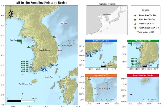
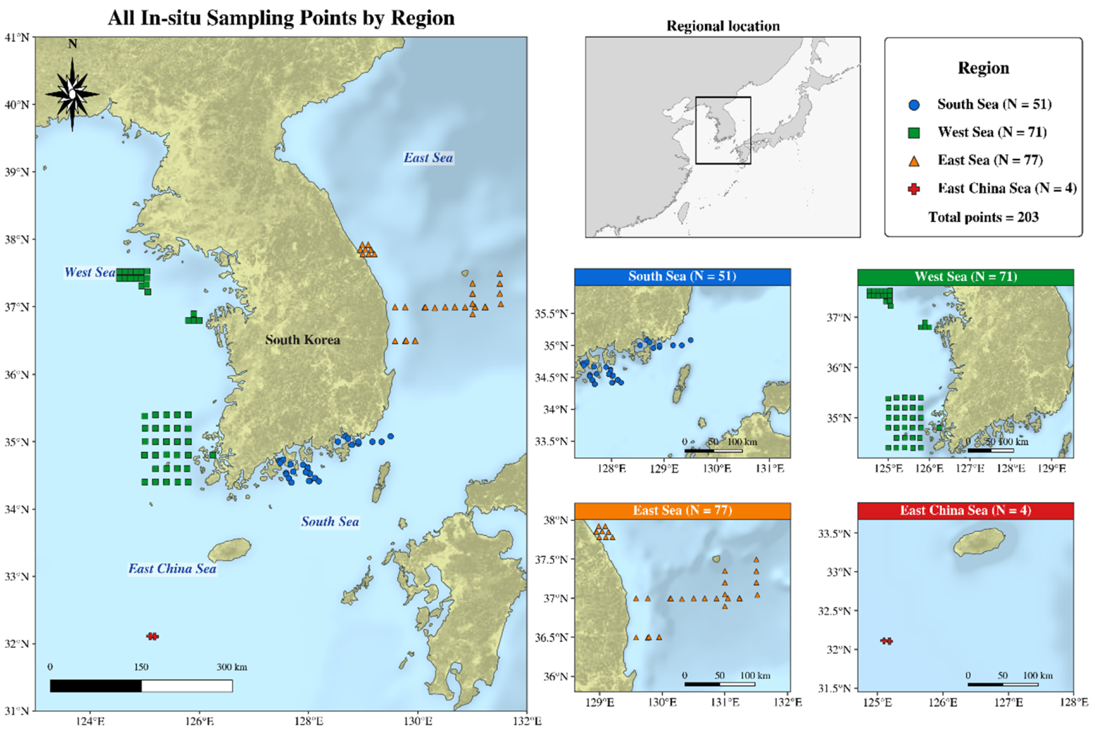
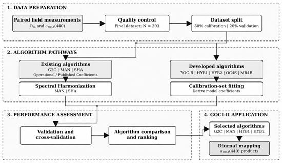
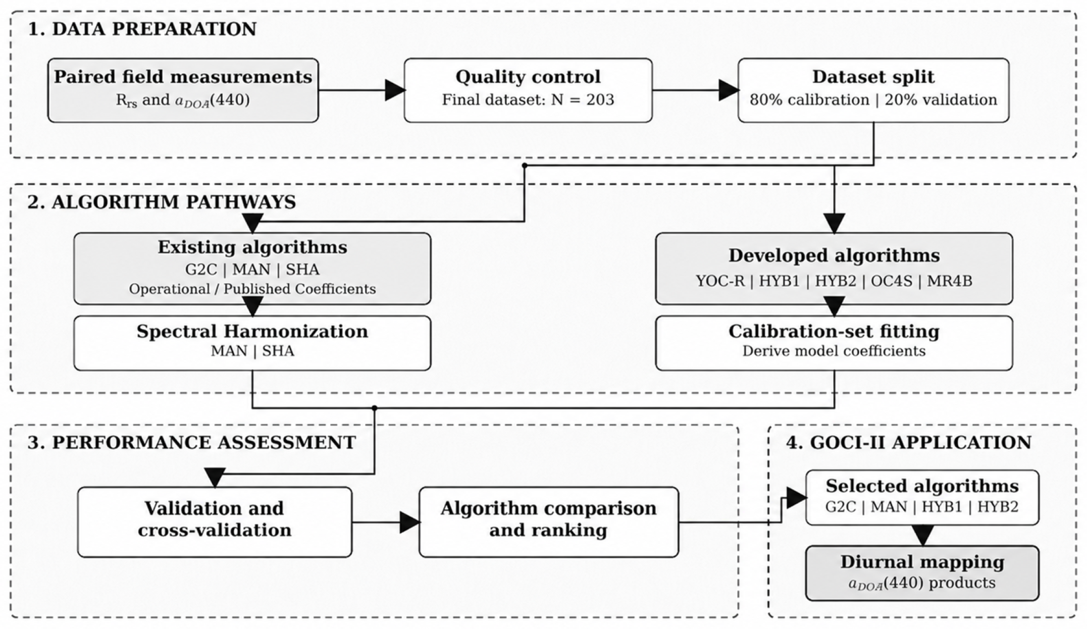
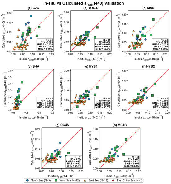
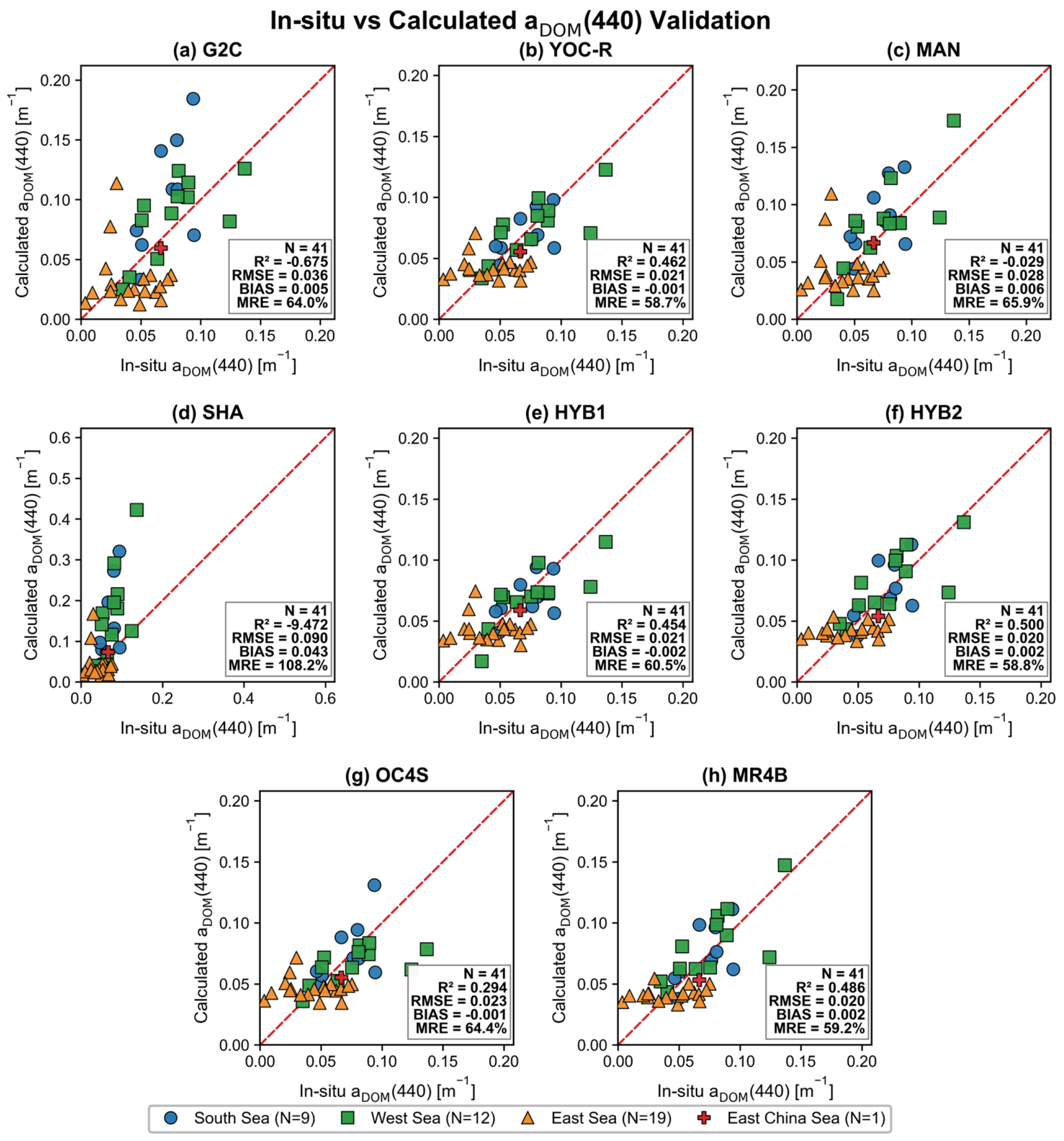
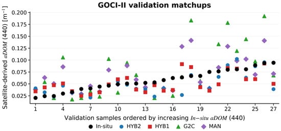
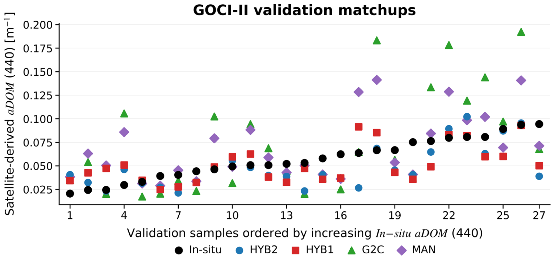
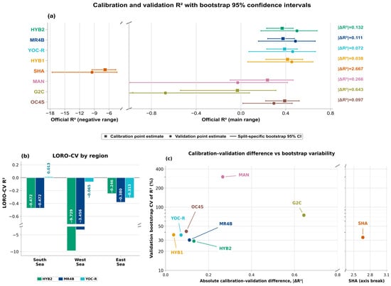
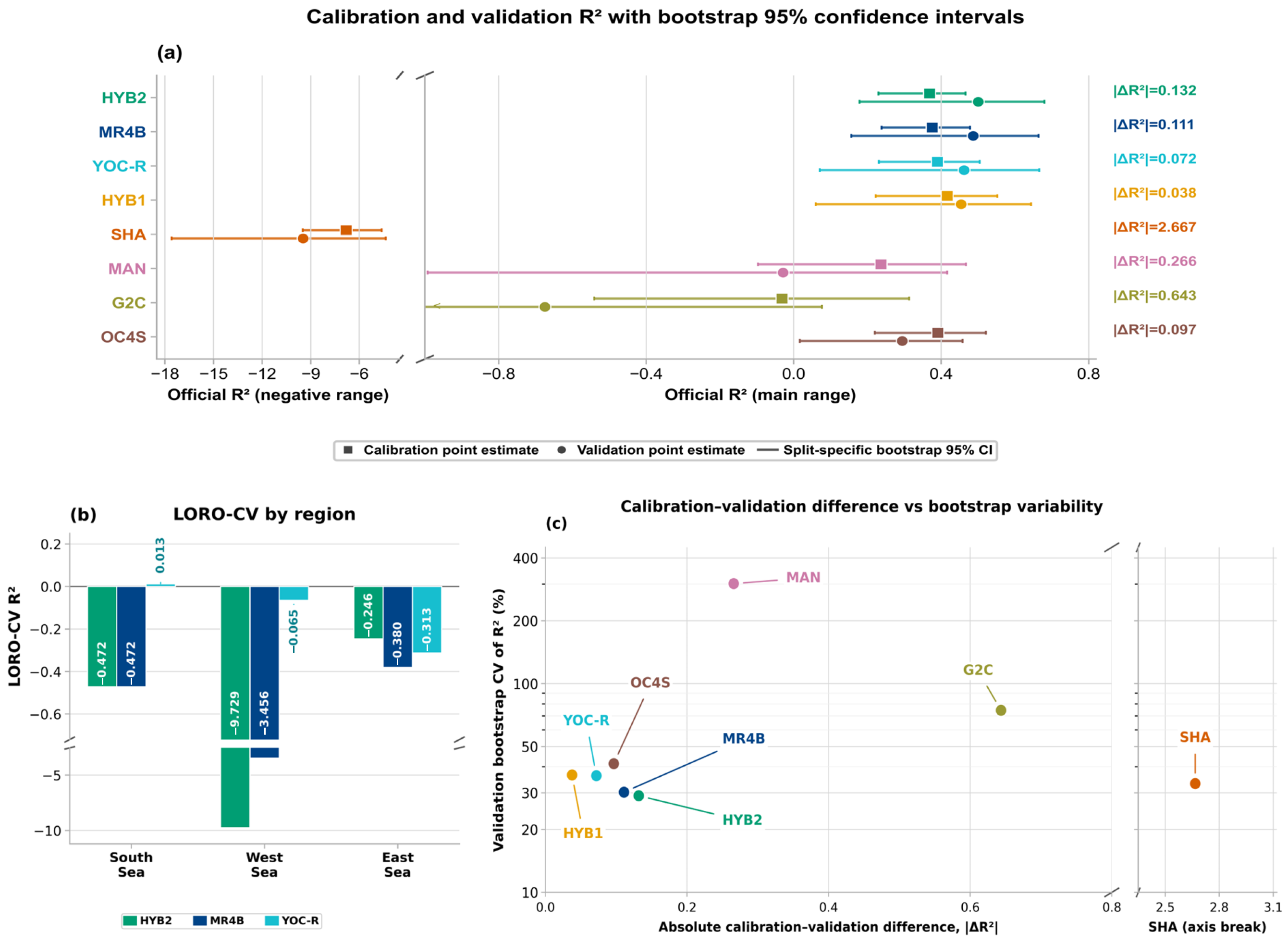
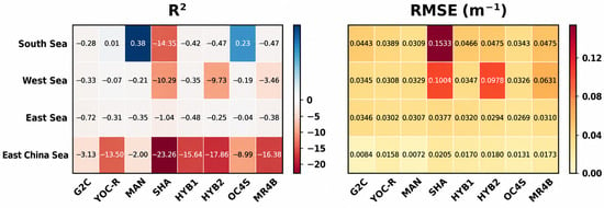
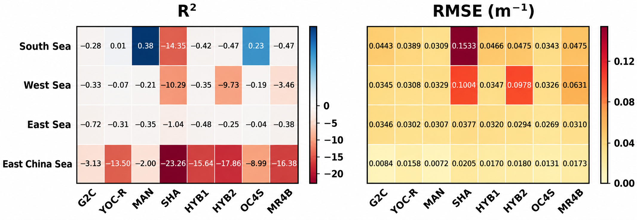
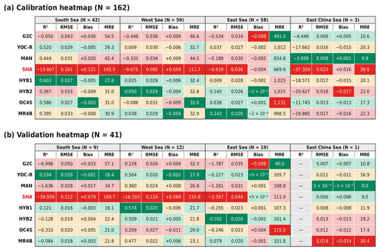
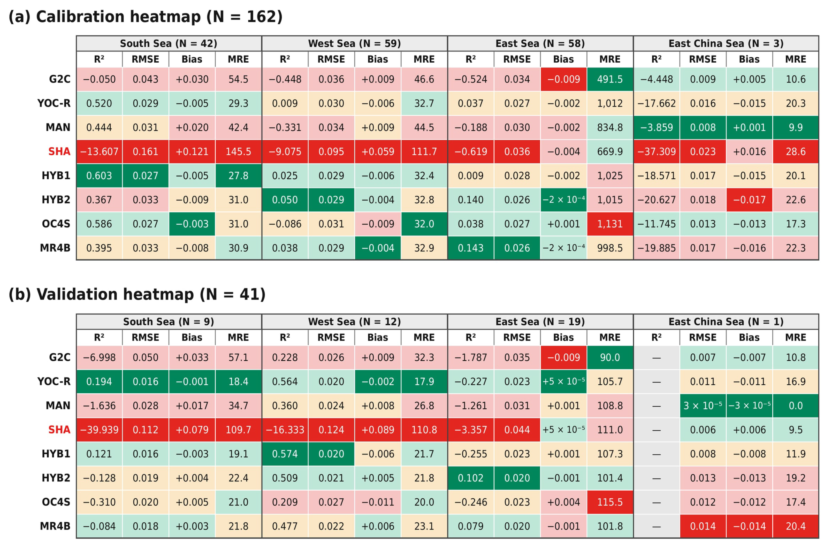
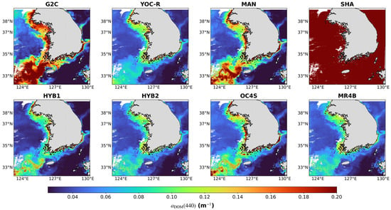
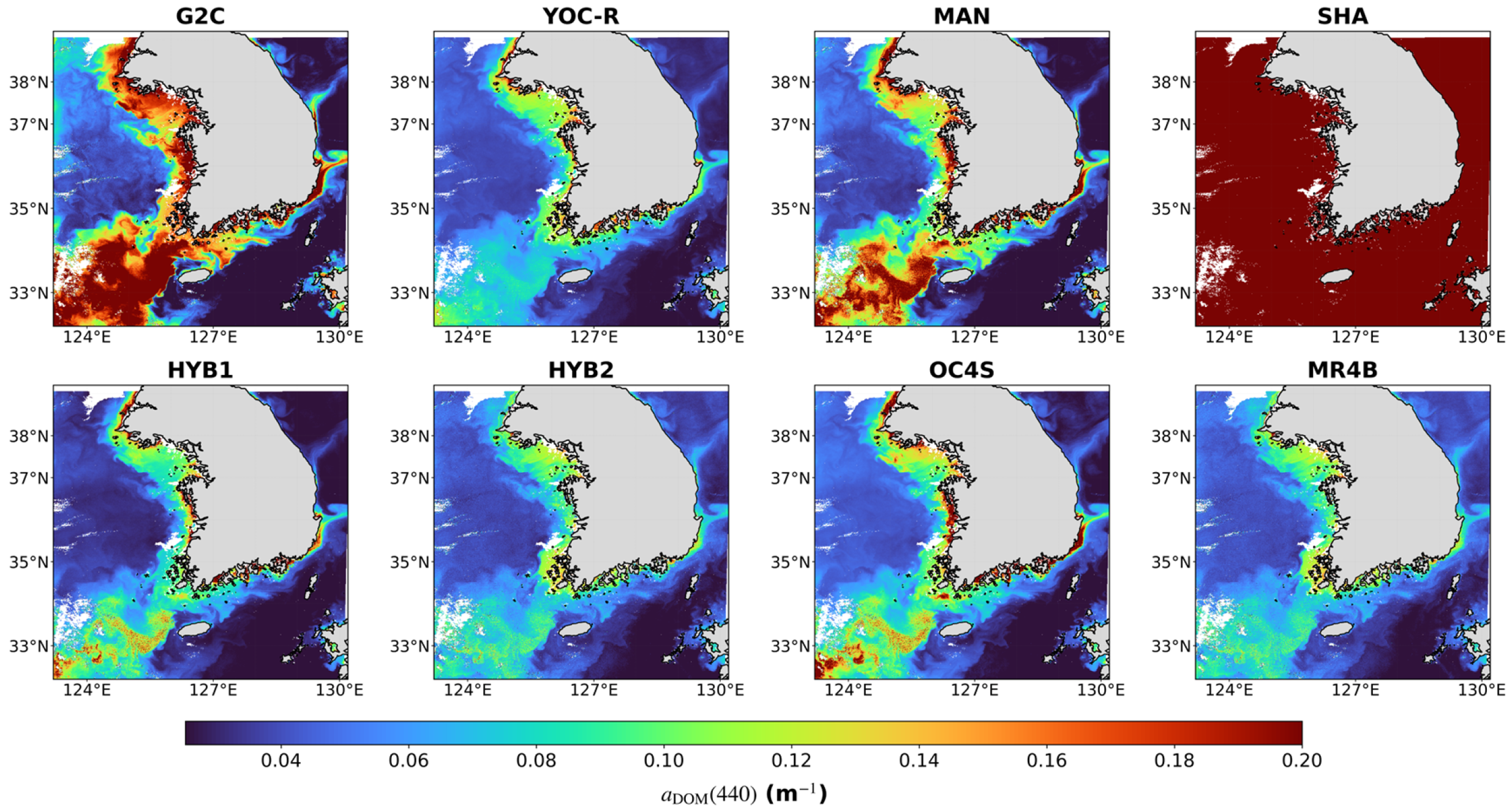
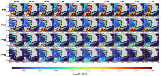
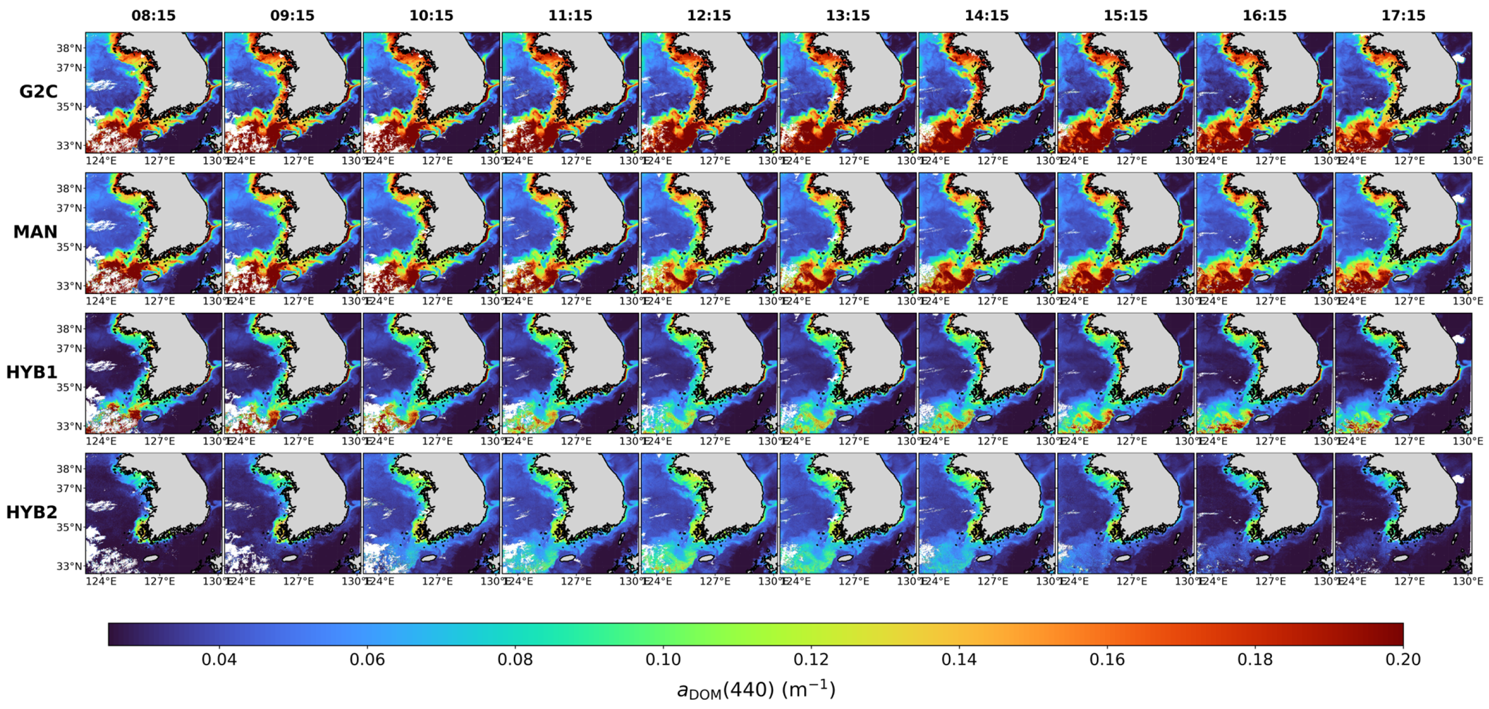

Disclaimer/Publisher’s Note: The statements, opinions and data contained in all publications are solely those of the individual author(s) and contributor(s) and not of MDPI and/or the editor(s). MDPI and/or the editor(s) disclaim responsibility for any injury to people or property resulting from any ideas, methods, instructions or products referred to in the content. |
© 2026 by the authors. Licensee MDPI, Basel, Switzerland. This article is an open access article distributed under the terms and conditions of the Creative Commons Attribution (CC BY) license.