


Highlights
What are the main findings?
- •
- Simulated CHIME hyperspectral data reproduce the principal spatial patterns of turbidity and related indices observed by Sentinel-2 and Landsat 8/9 while providing continuous spectral signatures that resolve spectral variability not represented by conventional multispectral bands. This additional spectral information supports a more detailed characterization of optically detectable water conditions, although the identification of individual contaminants and their sources was not directly assessed.
- •
- LSTM-simulated thermal data processed with a quadratic split-window model recover surface temperatures that match Landsat Band-10 references with operational accuracy (RMSE typically <1 °C and near-zero residual bias), outperforming both raw brightness temperatures and linear corrections.
What are the implications of the main findings?
- •
- Simulated CHIME and LSTM observations provide a basis for preparing future Copernicus water-monitoring workflows before mission launch. CHIME contributes continuous spectral information that supports the characterization of water-reflectance variability and turbidity-related spatial patterns, while LSTM contributes complementary information on surface-temperature variability. Together, these observations provide complementary optical and thermal information that may support future multisensor detection and characterization of discharge-related water-quality anomalies. The magnitude of this potential improvement was not quantified in the present study.
- •
- Pre-launch CHIME and LSTM simulations already meet quantitative realism criteria (structural similarity for optical patterns and thermal RMSE/bias thresholds) and therefore provide a credible basis for developing and validating multi-sensor water-anomaly and liquid-discharge monitoring applications before the missions become operational.
- •
- Integrating these future hyperspectral and thermal observations with existing multispectral sensors within a virtual-constellation framework enhances the detection, spectral characterization, and temporal coverage of discharge-related water-quality anomalies across coastal, lake, and riverine environments.
Abstract
The use of Earth Observation data for monitoring of aquatic and coastal ecosystems has expanded significantly, yet gaps remain in the spectral and thermal capabilities needed to detect and characterize liquid discharges. This study evaluates the potential of simulated pre-launch CHIME and LSTM observations, integrated with operational Sentinel-2 and Landsat 8/9 data, for water-quality anomaly detection across diverse aquatic environments, demonstrating that the simulated datasets are sufficiently realistic to reproduce key water-quality and thermal indicators and support pre-operational application development prior to mission launch. A multi-stage workflow was applied: initial anomaly detection with multispectral imagery, thermal verification using LSTM-simulated brightness temperatures processed via linear and quadratic split-window algorithms, and spectral characterization of turbidity and spectral signatures with atmospherically corrected CHIME-simulated data. Results showed consistent spatial patterns of turbidity and surface temperature between simulated and operational products, with CHIME resolving finer spectral features of suspended matter and the quadratic LSTM model achieving low RMSE relative to Landsat thermal references. These findings demonstrate the cross-sensor consistency and complementary information provided by simulated CHIME and LSTM products, supporting their use in the pre-launch development of future multisensor workflows for detecting and characterizing optical and thermal water anomalies. Identification of specific contaminants and attribution of anomalies to individual discharge sources were not assessed in this study.
1. Introduction
The use of Earth Observation (EO) data for the management and monitoring of aquatic and coastal ecosystems has become increasingly widespread. Remote sensing plays a key role in providing spatially and temporally distributed data, particularly in areas where traditional field measurements are difficult to obtain, thereby enabling the monitoring of the spatiotemporal dynamics of inland and coastal water biophysical properties. Satellite remote sensing has become an important tool for monitoring water quality, providing information on the spatial and temporal variability of aquatic environments that can complement conventional in situ measurements.
Early and widely used missions such as Landsat established the potential of multispectral satellite observations for monitoring inland and coastal waters, particularly through the detection of changes associated with suspended matter, turbidity, and water colour. The development of higher-resolution sensors (IKONOS, QuickBird, GeoEye-1, etc.) improved the ability to characterize spatially heterogeneous water bodies and identify water-quality patterns at relatively fine scales. Conversely, sensors such as MODIS, MERIS, SeaWiFS, and VIIRS have provided broader spatial coverage and frequent observations, making them particularly valuable for monitoring water-quality dynamics over large lakes, coastal zones, and oceanic environments. The availability of hyperspectral observations has also demonstrated the potential of detailed spectral information for retrieving and characterizing water-quality parameters. Overall, the evolution of satellite sensors has expanded the capacity to monitor water quality across different spatial and temporal scales, supporting the assessment of parameters such as turbidity, suspended sediments, chlorophyll-a, and algal blooms [1].
To improve environmental monitoring and support the sustainable management of natural resources, the European Space Agency (ESA) is developing a series of new Copernicus Next Generation Missions. These missions aim to address gaps identified in the Copernicus user requirements, expand the current capabilities of the Copernicus Space Component, and enhance Earth observation activities. Among these future missions are the Copernicus Hyperspectral Imaging Mission for the Environment (CHIME) and the Copernicus Land Surface Temperature Monitoring (LSTM) mission [2].
CHIME is designed to acquire high-resolution hyperspectral imagery that will support a broad range of applications, including precision agriculture, forest monitoring, raw materials exploration, biodiversity assessments, and water resource management [1]. LSTM will provide high-resolution Visible Shortwave Infrared (VSWIR) and Thermal Infrared (TIR) observation capabilities over land and coastal areas. The main objective of this mission is to retrieve land surface temperature and emissivity with sufficient spatial and temporal resolution to estimate field-scale evapotranspiration and water productivity. In addition, the mission will support a wide range of environmental applications, including coastal zone monitoring [3].
This hyperspectral sensor will consist of two identical satellites (CHIME-A and CHIME-B), each carrying an advanced HyperSpectral Imager (HSI) instrument. This sensor is designed to capture imagery in over 200 bands spanning 400–2500 nm, covering the visible (VIS), Near-Infrared (NIR), and Short-Wave Infrared (SWIR) spectral regions, with a spectral resolution of less than 10 nm. The mission will operate at a spatial resolution of 30 m and a swath width of 130 km, ensuring high radiometric accuracy with a revisit time of 10–12.5 days, using a sun synchronous orbit with an overpass time between 10:30–11:30 Local Time on Descending Node [4,5,6]. LSTM will carry a TIR instrument operating across the Visible and Near Infrared (VNIR), SWIR, and TIR spectral bands, with a spatial resolution of 50 m. This provides a substantial improvement over, for example, Sentinel-3 (spatial resolution of 1 km). The instrument will include five spectral bands in the 8–12.5 µm range, designed to cover a wide temperature range from –20 to 30 °C with a measurement precision of 0.3 °C [7].
Although the two missions are designed to address distinct primary objectives, their complementary spectral and thermal capabilities make them well suited to the investigation of liquid discharges, which can produce optical, thermal, or combined signatures. As CHIME and LSTM have not yet become operational, representative pre-launch datasets are needed to develop applications that can take advantage of their anticipated capabilities. Satellite data simulation offers an effective approach for reproducing the expected characteristics of future observations, thereby enabling the development, testing, and evaluation of methodologies prior to the missions’ launch [8].
In this study, we explore the suitability of these simulated datasets for real-world applications related to water-discharge monitoring in coastal waters, inland lakes, and riverine environments. The datasets consist of high-fidelity pre-launch proxy data generated by integrating physics-based radiative transfer modeling with deep learning architectures [8], providing a realistic representation of the expected CHIME and LSTM observations prior to the availability of operational mission data. The early involvement of end users is a key component in the development of future Earth observation (EO) applications, as it helps align emerging satellite capabilities with practical requirements for environmental monitoring.
This approach is adopted by the Multisensor Water Discharges (MWD) project, conducted within the European Space Agency’s (ESA) Sentinel User Preparation initiative. This user-driven approach provides a basis for assessing the consistency and potential applicability of the simulated products under conditions relevant to operational water monitoring, without assuming that the composition or source of individual discharges can be determined from the satellite observations alone. To support this objective, the study integrates simulated datasets representative of the hyperspectral measurements expected from CHIME with the thermal observations anticipated from LSTM. These datasets are used within a set of application scenarios developed together with operational end users, covering a range of monitoring objectives, discharge characteristics, and aquatic settings. This user-driven approach provides a basis for assessing the practical value of the combined missions under conditions representative of real-world monitoring activities.
This study investigates the potential integration of simulated CHIME and LSTM ob-servations with currently available Sentinel-2 and Landsat products within a future virtu-al-constellation framework for aquatic applications. Rather than attempting to quantify the full performance of such a constellation, the present analysis focuses on a necessary preliminary step: assessing the cross-sensor consistency and complementarity of the simulated products relative to operational satellite observations.
In this framework, CHIME and Sentinel-2 contribute information in the reflective spectral domain, whereas LSTM and Landsat provide complementary thermal observations. The joint availability of these observations potentially offers additional opportune-ties for characterizing dynamic aquatic processes; however, the quantitative gain resulting from their combined temporal sampling is not directly assessed by the pairwise comparisons performed here.
In this study, the term “virtual constellation” is used in a broader sense than increased revisit frequency alone. It also refers to the coordinated exploitation of complementary observations, particularly reflective/hyperspectral information relevant to water-quality characterization and thermal observations describing surface-temperature variability. The present study primarily addresses the cross-sensor compatibility required to support such future combined exploitation.
The objective of this study is to evaluate whether these pre-launch datasets, considered together with Sentinel-2 and Landsat 8/9 observations within a future virtual-constellation framework, can support the detection and spectral or thermal characterization of water-quality patterns and potential anomalies across coastal, lake, and riverine environments. This aim is addressed through four research questions: (i) assess the consistency of simulated CHIME observations with operational multispectral observations for the considered aquatic applications; (ii) assess the consistency of simulated LSTM-derived surface-temperature observations with existing Landsat products; (iii) investigate the suitability of the simulated datasets as proxies for developing multi-sensor aquatic-monitoring workflows ahead of the future missions; and (iv) discuss their potential integration with existing observations within a future virtual-constellation framework.
2. Materials and Methods
2.1. Study Sites
The study comprises six study sites representing three main aquatic environments in northern and southern Italy (Figure 1): three coastal and marine sites (Gulf of Manfredonia, Gulf of Taranto, and Coast of Bari), two lake sites (Centro Cadore Lake and Morto Lake), and one metropolitan riverine site (Lambro River).
Figure 1.
Location map of the selected Italian study sites (A–F). Red bounding boxes/polygons in the inset maps define the spatial extent of the analyzed domains: (A) Lambro River, (B) Lago Centro di Cadore, (C) Lago Morto, (D) Manfredonia/Ofanto mouth, (E) Bari offshore, and (F) Taranto Gulf coastal area. Coordinates are displayed in the main map grid (UTM).
These three groups were selected to represent a range of water conditions, allowing the assessment of the potential applications and limitations of CHIME- and LSTM-simulated data under realistic environmental settings, including varying water conditions; land–water boundaries; and anthropogenic influences such as industrial discharges, urban heat effects, cooling-water outlets, etc.
The Gulf of Manfredonia is a large, shallow embayment located in the western sector of the southern Adriatic Sea (Figure 1A). Its seafloor exhibits a marked increase in bathymetric gradient from depths of approximately 30 m toward the shoreline, primarily due to sediment transport driven by the northern Adriatic current. The coastal marine environment of the gulf is subject to multiple anthropogenic pressures, including agricultural, industrial, and urban activities [9]. The Taranto Gulf is a large square-shaped gulf of 140 by 140 km located in the northwestern part of the Ionian Sea (Figure 1B). The gulf, as the other one, is named after the town of Taranto. The seafloor morphology in this zone is characterized by the Taranto Valley. In this case, the coastal and marine ecosystems have been altered by industrial factories of steel and iron (being Ilva the most important steel production plant in Europe), petroleum refineries, and intensive marine traffic. The last area of this group, Bari, is located on the southeastern Adriatic coast, in the center of the Apulia region. It has a low-profile morphology characterized mainly by sandy sediments, with most of its coastline and beaches only partially preserved due to human intervention. Its port is one of the most important ports on the Adriatic Sea and is located within the urban area of the Metropolitan City of Bari. The water depth varies from 6.9 to 14.9 m, allowing the movement of large ships and vessels [10].
The Lambro River, one of the most polluted tributaries of the Po River, stretches 133 km. It flows through one of the most densely populated regions of Lombardia, including the Milan metropolitan area. The river receives effluents from over 30 wastewater treatment plants, along with numerous artificial and natural tributaries. This area is also home to one of Europe’s highest population densities, with a river that supports a highly developed industrial sector, including textile, paper, and food production [9,11]. The Lake of Centro Cadore, located within the Belluno province of Italy, is a significant artificial reservoir constructed between 1946 and 1949. The reservoir is enclosed by a dam situated at ‘Pian delle Ere’ and spans across four municipal territories in the region. At its maximum capacity, the lake stretches for 9.3 km and is primarily fed by the Piave River [12].
Finally, Lago Morto, located in the province of Treviso, Veneto, northern Italy, lies at an elevation of approximately 274 m above sea level. It is one of the three main lakes situated along the axis of the valley, together with Restello Lake and Negrisiola Lake. All three lakes are artificial reservoirs used for hydroelectric power production. This Lake is particularly interesting because it is not fed by a major surface river; instead, its water comes mainly from underground infiltration from Lago di Santa Croce. The lake is also supplied by karst springs located along the right side of the valley, particularly the Vallon della Fontana Spring [13].
The study sites were selected to increase the probability of detecting anomalies by considering the characteristics of each water body and its associated vulnerability factors. The selected sites encompass different aquatic environments, including riverine habitats with narrow geometries, lakes with constrained spatial configurations, and coastal waters. These contrasting environments and their respective anthropogenic pressures provide a range of conditions in which potential anomalies may occur. Table 1 summarizes the main anthropogenic impacts and potential vulnerability factors reported for each study site.
Table 1.
Study sites and potential factors influencing anomaly detection.
2.2. Data
2.2.1. Remote Sensing Data
A comprehensive search was conducted across the archival catalogs of relevant Earth Observation (EO) missions to ensure thorough data coverage. The search encompassed not only hyperspectral missions but also relevant multispectral archives, as well as simulated datasets representing the observational capabilities of forthcoming EO missions. The objective was to identify and retrieve all available datasets corresponding to the selected study sites that could support the analysis. To this end, a period of 3 days will be considered for the selection of this multispectral data (1—the day before, 2—the same day, 3—the day after) to select images that could be paired with hyperspectral data. Table 2 summarizes the spectral range, number of bands, GSD, and temporal resolution of the sensors considered in this study for the workflow proposed for anomaly detection. Detailed technical information will be given at the preprocessing and processing section of the methodology of the sensor used for the study.
Table 2.
Technical specifications of data/simulated data and review used in this study.
A complete inventory of the satellite acquisitions and their associated metadata is provided in Table A1.
2.2.2. Simulated Remote Sensing Data
The hyperspectral simulated optical data used in these analyses comprise observations from two hyperspectral sensors, PRISMA and EnMAP. Both sensors provide observations with high spectral resolution across the VNIR and SWIR domains, making them suitable precursor datasets for generating observations representative of the future CHIME mission. For the simulated thermal hyperspectral data, representative LSTM products were generated from Landsat thermal data. The methodology used to generate the representative CHIME and LSTM-simulated datasets and used sensors is described in detail in Koutsantoni et al. [8]. Table 3 provides the technical specifications of all the sensors used to generate the simulated datasets, including both optical and thermal sensors. In the present study a total of 48 CHIME-Sim, and 16 LSTM-Sim Day acquisitions were reviewed. These simulated datasets used as inputs to the application/oriented analysis over the study sites relevant to the interpretation of the results are summarized in Appendix A Table A2.
Table 3.
Technical specifications of sensors used for the creation of the simulated data in this study (optical and thermal) [8].
Although some of the operational observations used in the comparative assessment are related to the data sources employed in constructing the simulated datasets, CHIME-Sim and LSTM-Sim are generated through dedicated simulation procedures intended to reproduce the characteristics of the respective future sensors and are therefore not direct replicas of the original observations. Consequently, independence should be considered at two levels: observational independence, which is not complete for all comparisons, and methodological independence introduced by the simulation and sensor-transfer procedures. The comparisons presented here are therefore primarily interpreted as tests of cross-sensor consistency and proxy-data suitability, while also providing supporting evidence for the physical plausibility of the simulated observations. They are not intended as a substitute for fully independent validation of the quantitative and operational accuracy of future CHIME and LSTM observations.
2.2.3. River Forecast System Data
Due to the limited hydrological data available for some tributaries within the study sites, the Group on Earth Observations Global Water Sustainability (GEOGLOWS) Streamflow Service was used. GEOGLOWS Streamflow Service is a global hydrological forecasting system that provides historical and forecasted river discharge information. The system combines land-surface modelling, runoff generation, and river-routing techniques to produce streamflow estimates for rivers throughout the world [26]. The GEOGLOWS River Forecast System (RFS), Hydrologic Model Version 2, is a global hydrological forecasting system that provides historical and forecasted river discharge. It combines TanDEM-X-derived hydrography (TDX-Hydro) with ECMWF ERA5 reanalysis for historical simulations and IFS forecasts for future forcing. GEOGLOWS RFS provides river-reach-specific streamflow simulations and forecasts, including historical discharge, 15-day ensemble forecasts, and return-period flow estimates, allowing hydrological conditions to be assessed for individual tributaries within the study area [27].
2.3. Methods
The overall workflow of the methodology adopted in this research is illustrated in Figure 2 and consists of three main stages. The first stage of the processing pipeline focuses on the initial detection of discharges using Sentinel-2 and Landsat 8/9 imagery to enable broad-scale monitoring. The second stage incorporates simulated LSTM data to reduce false alarms and improve detection accuracy. Finally, the third stage uses simulated CHIME hyperspectral data, where available, to characterize the spectral signatures and spectral indices associated with the identified water anomaly. However, this three-stage workflow is not directly applicable to all types of water bodies. In particular, the identification of anomalies in rivers and in most small water bodies within the study areas can be challenging because of their limited spatial dimensions, with river widths generally ranging between 30 and 100 m. The use of LSTM in these environments would provide limited benefit because of its spatial resolution. Consequently, these water bodies will not be processed through the complete three-stage workflow. Instead, their analysis will rely on the combined exploitation of MSI (Sentinel-02/Landsat08/09) and CHIME data. Nevertheless, even with the 10 m spatial resolution of Sentinel-2, 30 m spatial resolution of Landsat, and the 30 m resolution of CHIME, anomaly detection cannot reliably be based on the identification of spatial edges or gradients between anomalous and non-anomalous river water. The analysis will therefore focus on the spectral characteristics of the water pixels, using MSI for the initial identification of potential anomalies and CHIME, where available, for the subsequent characterization of spectral variability.
Figure 2.
Schematic overview of the three-stage processing workflow: initial detection using Landsat-08/09 and Sentinel-2 (MSI), thermal verification with LSTM-simulated TIR data (HSI), and spectral characterization using CHIME-simulated optical data (HSI) to inform water management decision-making.
2.3.1. Spectral Methods
Band Ratio
Spectral band ratio methods use a simple semi-empirical approach to estimate water quality parameters by creating a mathematical ratio between the reflectance of two or more spectral bands [28]. The basic relationship can be describe as described by:
where is the quantity of the parameter being estimated; R1 is the reflectance in the band I; and α, β, and γ are the coefficients derived from regression. Ratio-based algorithms can incorporate multiple spectral band combinations to capture key features in the sensor’s reflectance data (Table 4). These ratios are commonly employed as predictor variables in regression models. Such approaches have been extensively investigated for estimating chlorophyll-a (Chl-a) concentrations, particularly through the reflectance ratio between 700 nm and 670 nm.
Table 4.
Spectral indices and band combinations.
Water Mask
A water index is designed to enhance the contrast between water and non-water pixels. By combining specific optical bands, these indices can accurately and robustly distinguish water bodies from other land cover types [1]. In this study, the McFeeters Normalized Difference Water Index (NDWI) was used. The NDWI takes advantage of the strong absorption of near-infrared (NIR) radiation by water and the high reflectance of vegetation and soil in the NIR band relative to the green band. Based on this principle, the NDWI is defined as
where ρGreen and ρNIR are the Top-of-Atmosphere (TOA) reflectance of the green and near-infrared bands, respectively. Water bodies generally exhibit positive NDWI values because of the strong absorption of NIR light relative to green light. In contrast, soil, vegetation, and built-up areas typically produce negative or near-zero values, as they reflect more NIR light than green light.
2.3.2. Selection and Pre-Processing of Multi-Spectral Images
Two constellations of multispectral satellites were included in the workflow for the initial detection of the water quality parameter across all study sites in this research. The first, Sentinel-2, is a European Earth observation mission developed under the Copernicus Program. Sentinel-2A was launched on 23 June 2015, followed by Sentinel-2B on 7 March 2017, and Sentinel-2C on 5 September 2024 (but this one, was not considered because fell outside the observation timeframe of the study). To ensure data consistency across the observation timeframe, imagery for this study was retrieved exclusively from Sentinel-2A and Sentinel-2B. The sensor provides 13 spectral bands covering a wavelength range from 443 nm to 2190 nm, with four bands at 10 m spatial resolution (VNIR), six bands at 20 m (red edge/SWIR), and three bands at 60 m (primarily atmospheric correction bands) [33,34].
The other constellation corresponds to Landsat 08/09 for this initial detection and assessment of the water quality parameters across all study sites considered in this research. Landsat 08, launched on 11 February 2013, and Landsat 09, launched on 27 September 2021, are part of the joint NASA-USGS Earth Observation Program. Both satellites carry two complementary sensors, the Operation Land Imager (OLI) and the Thermal Infrared Sensor. The sensors provide observations across the visible, near-infrared (VNIR), shortwave-infrared (SWIR), and thermal-infrared (TIR) portions of the electromagnetic spectrum. The Operational Land Imager (OLI) acquires nine spectral bands covering wavelengths from approximately 443 nm to 2290 nm, with seven multispectral bands at 30 m spatial resolution and one panchromatic band at 15 m, while the Thermal Infrared Sensor (TIRS) provides two thermal bands centered at approximately 10.9 and 12.0 µm, with a native spatial resolution of 100 m that is resampled to 30 m in standard products [35].
In this study, the selection and pre-processing of suitable Sentinel-2 and Landsat 8/9 images were performed using the Google Earth Engine (GEE) platform. GEE is a cloud-based computing platform launched in 2010 to support large-scale geospatial analysis. It provides access to a vast repository of publicly available satellite datasets, including Sentinel and Landsat collections. Furthermore, GEE offers a parallel processing capability that distributes computational tasks across high-performance servers, enabling the rapid processing of hundreds of images within seconds [36]. Importantly, the entire analysis can be conducted directly on the platform without the need to download the data locally.
2.3.3. Selection and Pre-Processing of Hyperspectral Images
Two Hyperspectral simulated satellite databases were included to continue with the proposed workflow for the detection of anomalies in the water quality parameters. The first one, CHIME, will provide observations across the visible (VIS), near-infrared (NIR), and shortwave-infrared (SWIR) regions of the electromagnetic spectrum. The mission will carry a hyperspectral imaging instrument covering approximately 400–2500 nm, acquiring more than 200 contiguous spectral bands with a spectral sampling of 8.4 nm. CHIME is designed to provide a spatial resolution of 30 m and a swath width of approximately 130 km [5].
The second one, LSTM, will provide high-resolution observations in the thermal-infrared (TIR) region for the monitoring of land-surface temperature and evapotranspiration. The mission will carry a high-resolution thermal infrared instrument covering approximately the 8–12.5 µm spectral range, with multiple thermal bands designed to characterize surface temperature and emissivity. LSTM is designed to provide a spatial resolution of approximately 50 m and a temperature measurement accuracy of approximately 0.3 K [5].
In this study, the analysis was performed using CHIME-simulated hyperspectral data and LSTM-simulated thermal infrared data generated within the Multisensor Water Discharges project. A detailed description of the methodology adopted to generate these simulated datasets is provided in [8]. The simulated datasets are publicly available through the project repositories hosted on the European Space Agency (ESA) APEX platform at [CHIME-Sim = https://browser.apex.esa.int/external/eoresults.esa.int/stac/collections/mwd-chime-sim?.language=en (accessed on 5 October 2026), LSTM-Sim = https://browser.apex.esa.int/external/eoresults.esa.int/stac/collections/mwd-lstm-sim (accessed on 5 October 2026)]. These datasets were used as the initial input for the present analysis and were processed locally using Python 3.9.13 within Jupyter Notebook environments. The processing workflow included atmospheric correction of the satellite observations, preparation and quality control of the resulting datasets, extraction of the relevant spectral and thermal information, and subsequent analysis of water-quality and surface-temperature parameters. This approach enabled the publicly available simulated datasets to be processed according to the specific objectives and methodological requirements of the present study.
2.3.4. Solar Irradiance Model: TOA Radiance to TOA Reflectance
Conversion of Top-of-Atmosphere (TOA) radiance to TOA reflectance was performed using the TSIS-1 Hybrid Solar Reference Spectrum (HSRS) version published by Coddington et al. [37]. This spectrum was selected because of its high radiometric accuracy and full spectral coverage (202–2730 nm), making it suitable for the CHIME spectral range. Band-equivalent extra-terrestrial solar irradiances E0(λ)were obtained by convolving the high-resolution TSIS-1 HSRS (0.01 nm resolution) with a Gaussian approximation of the CHIME spectral response function for each of the 251 bands. The Earth–Sun distance factor d was computed from the acquisition date following standard astronomical formulae. The spectral radiance is derived by scaling the raw digital number (DN), using the instrument radiometric scaling factor:
where LTOA,i is the calibrated Top-of-Atmosphere spectral radiance for band i, DNi is the raw digital number for band i, and k is the gain scaling factor (10−4 W ⋅ m−2 ⋅ sr−1 ⋅ nm−1). The conversion from calibrated TOA radiance L(λ) to dimensionless TOA reflectance ρTOA(λ) followed the conventional formulation:
where ρTOA,i is the Dimensionless Top-of-Atmosphere spectral reflectance; π is the mathematical standard Archimedes constant (), representing the conversion of the directional radiance to total exitance flux; LTOA,i represents the At-sensor Top-of-Atmosphere spectral radiance per band (W ⋅ m−2 ⋅ sr−1 ⋅ nm−1); d represents the Instantaneous Earth–Sun distance in AU ratio; F0,i is the band-averaged mean extra-terrestrial solar irradiance; and θs is the Solar Zenith Angle (radians). This approach is consistent with the processing protocols applied to PRISMA data [38] and ensures radiometric compatibility with other optical sensors used in the virtual constellation analysis.
These calculated F0,i band average mean value with the dimension of the uncertainty per band are summarized in the Appendix B Table A3 for replicability purposes. To account for the spectral response of the CHIME instrument, the band-equivalent extra-terrestrial solar irradiance E0(λi) for each of the 251 spectral bands was synthesized by convolving the high-resolution TSIS-1 Hybrid Solar Reference Spectrum Esun(λ) with a normalized Gaussian Spectral Response Function (SRF).
where is the unnormalized Gaussian spectral response profile for spectral channel i (dimensionless), λ is the continuous optical wavelength (nm), λi is the nominal central wavelength for band i (nm) and σ is the spectral standard deviation of the Gaussian channel response (nm). Then the spectral gaussian standard deviation was calculated by the formula:
where σ is the spectral standard deviation (≈4.2466 nm/CHIME), FWHM is the Full Width at Half Maximum of the spectral channel (10.0 nm) and ln2 is the natural logarithm of 2. Then the Normalized Spectral Response Function (Si) is calculated by:
where Si(λ) is the area-normalized Spectral Response Function (nm−1), gi(λ) is the unnormalized Gaussian spectral response for band i; λ′ is the integration variable over wavelength (nm), [λmin,λmax] is the operational spectral domain bounds of the sensor (nm). Finally, the band-equivalent mean exo-atmospheric solar irradiance at standard mean Earth–Sun distance is computed by integrating the high-resolution reference solar irradiance spectrum Esun(λ) weighted by Si(λ). The numerical integration is executed using Simpson’s composite rule over a bounded spectral window defined at ±3.5σ centered around λi [39]:
The numerical integration was performed using Simpson’s composite rule over a spectral window of ±3σi centered on λi. This window captures more than 99.7% of the Gaussian response energy while avoiding spectral truncation artefacts outside the active channel passband.
2.3.5. Atmospheric Correction CHIME-Sim: Dark Object Subtraction for Water Bodies (DOS-W)
To retrieve Bottom-of-Atmosphere (BOA) surface reflectance (ρs) from the CHIME Level-1B Top-of-Atmosphere (TOA) reflectance cube (ρTOA), a dedicated aquatic simplified atmospheric correction was implemented based on dark-object subtraction over water pixels [40]. Standard land-oriented atmospheric correction models frequently overestimate aerosol reflectance over inland and coastal aquatic targets due to residual background haze and diffuse skylight reflection. Because clear water is among the darkest targets in the visible and near-infrared spectrum, the lowest reflectance values recorded over pure water pixels were treated as an estimate of atmospheric path reflectance ρpath. The workflow proceeds as follows. First, a clear-water spatial mask (Mwater) is generated using the Normalized Difference Water Index (NDWI) together with a Near-Infrared threshold [32]:
where NDWI corresponds to the Normalized Difference Water Index, ρTOA, green corresponds to TOA reflectance in the green band, ρTOA, NIR correspond to the TOA NIR band, the threshold of NDWI > 0.10 identifies pixels with relatively strong water-like spectral behavior and NIR < 0.035 is an additional threshold requiring very low NIR reflectance, which is characteristic of clear/open water. For each spectral band bρTOA, green
where ρTOA,b corresponds to the TOA reflectance in band b at pixel (x, y); Mwater corresponds to the Mask water valid pixels; (x,y) ∈ Mwater corresponds to the select pixel only classified as water; P5( ) corresponds to the 5th percentile of the selected reflectance values, consistent with the approach of Sobrino et al. [41]; and ρpath,b corresponds to the estimated path reflectance for band b. Surface reflectance is then obtained by subtracting 95% of the estimated path reflectance and enforcing a non-negativity floor:
where ρs,b(x,y) corresponds to the estimated surface reflectance at pixel (x, y), in spectral band b; ρTOA,b(x,y) corresponds to the measured top-of-atmosphere (TOA) reflectance; ρpath,b corresponds to the estimated path reflectance, obtained previously from the water pixels; 0.95 − 99 ρpath,b corresponds to the amount of atmospheric contribution that subtracted for the specific image; and ε corresponds to 0.0001 (the minimum allowed reflectance). The factor of 0.95–0.99 provides a similar conservative correction that avoids over-subtraction (as the Landsat or Sentinel-2 conservative-DOS program), with an exception of Morto Lake, where a more conservative factor of 0.80 was applied to account for atmospheric correction challenges in lakes. Such corrections are particularly difficult because strong reflectance from surrounding vegetation, especially in the NIR, can contaminate the signal from dark lake water through the adjacency effect, an impact that is especially pronounced in small lakes [42]. Under the constraints of pre-operational simulated CHIME data, for which the full suite of auxiliary atmospheric parameters required by advanced radiative-transfer-based processors is not yet available, this formulation retains only the additive path-radiance (haze) term. This is a simplification of the well-established DOS approach when the primary objective is the analysis of relative spatial patterns rather than the retrieval of absolute water-leaving reflectance values [43,44]. A simplified, image-based atmospheric correction was deliberately preferred over full radiative-transfer processors for three reasons: (i) the simulated CHIME and LSTM products lack the complete auxiliary atmospheric information required by operational algorithms; (ii) the primary objective of the study is the assessment of relative spatial patterns and cross-sensor consistency rather than absolute water-leaving reflectance; and (iii) this approach maintains methodological homogeneity across the optical and thermal domains, facilitating the virtual-constellation analysis.
2.3.6. Turbidity Retrieval: Nechad Model
Following atmospheric correction, turbidity (expressed in Formazin Nephelometric Units, FNU) was retrieved from the BOA surface reflectance using the single-band semi-analytical model defined by Nechad [45]. The algorithm relates water-leaving surface reflectance in the red band (λ = 644 nm) directly to total suspended particulate matter and turbidity through a non-linear calibration function [45]:
where T is the retrieved turbidity (FNU), ρBOA (λ) is the water surface reflectance at 644 nm, and A and C are wavelength-specific empirical calibration coefficients derived from field spectra. For the CHIME red wavelength used was Band 31, for Sentinel-02 MSI the band 4, and for Landsat 08/09 MSI the band 4, with the standard global calibration parameters proposed by Nechad et al. [45] were applied (A = 228.1 and C = 0.1641), and used by Dogliotti et al. [46], for the calculation of turbidity in coastal and estuarine waters These coefficients were selected because they have been extensively validated across a wide range of optical water types (clear to moderately turbid) and form the reference implementation in several operational processors, including ACOLITE (Atmospheric Correction for OLI-lite), and variants of C2RCC [47]. For the Coast of Bari, atmospheric correction of the MSI satellite imagery and subsequent Nechad turbidity retrievals were performed using the open-source ACOLITE processor (https://odnature.naturalsciences.be/remsem/software-and-data/acolite accessed on 5 October 2026). ACOLITE is an open-source processor designed for coastal and turbid waters that applies the Dark Spectrum Fitting (DSF) atmospheric correction, an advanced form of DOS, to Level-1 Landsat and Sentinel-2 imagery, retrieving reliable surface reflectance even in sediment-rich environments. It further implements the Nechad single-band turbidity algorithm, as mentioned above [47].
2.3.7. Spectral Signature and Spatial Comparison Metrics
To evaluate the cross-sensor agreement and fidelity between multispectral satellite observations (Sentinel-2/Landsat) and hyperspectral data, three complementary spectral distance metrics were calculated: Root Mean Square Error (RMSE), Spectral Angle Mapper (SAM), Structure Similarity Index Measure (SIM), and the Pearson Correlation. The RMSE is defined as the absolute difference in reflectance magnitude between the multispectral bands (MSi) and the corresponding simulated or resampled CHIME bands (CHIMEi) across N matched spectral channels is for the formula as [48]:
where MSi represents the surface reflectance of band i from the multispectral sensor (Sentinel-2 or Landsat), CHIMEi is the corresponding CHIME band reflectance, and N is the total number of evaluated bands. The Spectral Angle Mapper (SAM) corresponds to the spectral shape divergence between the two sensors and is computed by treating each spectral signature as a vector in an N-dimensional space. The angle between the multispectral vector and the CHIME vector (converted from radians to degrees) is given by [49]:
where a SAM value closer to 0° indicates high shape similarity between the spectral signatures, while lower RMSE values indicate closer absolute radiometric alignment. In addition, the Spectral Similarity Score (SS) was derived from the previous formula as:
where an SS of 1.0 indicates identical spectral shape, while lower values indicate increasing dissimilarity. This score is the metric commonly reported in water-quality spectral matching studies [50]. Unlike terrestrial targets, low-reflectance aquatic targets are highly sensitive to small atmospheric correction offsets, particularly in strongly absorbing NIR/SWIR bands. Following aquatic spectroscopy standards, a cosine similarity threshold of 0.80, corresponding to a maximum allowable spectral angle of 0.64 rad (~37°), is established as the baseline threshold for acceptable relative spectral shape agreement over water bodies. Spectral angles within the range of ≤0.45 rad (~26°) (SS ≥ 0.90) represent strong shape correlation in aquatic remote sensing [51,52]. Structural Similarity Index Measure (SSIM) is a perceptual metric used to quantify how similar two images or spatial grids are to one another. Unlike traditional error metrics (like RMSE or MAD) that compare pixel values independently, SSIM evaluates how human vision perceives spatial structural patterns, making it ideal for comparing satellite-derived spatial datasets. For two corresponding local image patches x and y:
where μx, μy are the local weighted mean values of patches x and y, are local weighted variances of x and y, σxy is the local weighted covariance between x and y, and and are stabilization constants to prevent division by zero, where default parameters use K1 = 0.01 and K2 = 0.03 []. Since the land-vs-water binary shape would be identical between grids and to avoid the artificial inflation of the final SSIM score with a massive area of a perfect match, the only validated pixels would be considered inside the water body itself. Finally, Spatial agreement between the products was quantified using the Pearson product-moment correlation coefficient [52], computed with SciPy’s pearsonr implementation on all valid water pixels by:
where xi and yi are the paired observations of the products, and are the respective sample means, and n is the number of valid pixels.
2.3.8. Temperature Brightness Retrieval
Brightness temperature was retrieved from the TOA spectral radiance using the inverse of Planck’s law. For each thermal band centered at wavelengths 8.6, 8.9, 9.2, 10.9, and 12.0 µm, the sensor radiance Lλ (in W m−2 sr−1 µm−1) was converted to brightness temperature Tb (in Kelvin) according to the following equation [53,54]:
where h is Planck’s constant, c is the speed of light, k is Boltzmann’s constant, and λ is the central wavelength in meters. The factor of 106 accounts for the conversion of spectral radiance units from per micrometer to per meter to maintain consistency with the SI formulation of Planck’s function. The resulting brightness temperatures were then converted to Celsius for visualization and analysis. This approach provides a direct physical conversion from measured radiance to equivalent blackbody temperature without atmospheric correction at this stage, allowing assessment of the raw thermal signal from the LSTM sensor over the study area.
2.3.9. Split-Window Surface Temperature Models
A split-window atmospheric correction technique was used to estimate true surface temperature by exploiting the differential atmospheric absorption observed across two adjacent thermal infrared spectral bands of the LSTM-Sim data, centered around 10.9 and 12.0 μm, respectively. Because water vapor absorbs thermal radiation at a slightly higher rate at 12.0 μm than at 10.9 μm, the difference between their measured TOA brightness temperatures, ΔT = T10.9 − T12.0, acts as an indirect proxy for the total atmospheric column water vapor and the associated path attenuation. The split-window method can effectively retrieve surface temperature by compensating for atmospheric path radiance and absorption, without requiring synchronous in situ atmospheric profile soundings, in this case, using a simplified version with atmospheric coefficients. Finally, we apply a linear and quadratic split-window atmospheric correction to examine the spatial coupling between retrieve surface temperature (Landsat/LSTM-Sim). Following the classical split-window approach for sea surface temperature retrieval, the sea surface was considered approximately as a blackbody (ε ≈ 1). Accordingly, no explicit surface-emissivity correction was applied in the present implementation [55]. Then, the atmospheric moisture signal is isolated by computing the differential brightness temperature between the two adjacent thermal bands [56]:
where ΔT is the brightness temperature differential between the two thermal bands, T10.9 is the brightness temperature measured in the 10.9 μm channel (lower water vapor absorption), and T12.0 is the brightness temperature measured in the 12.0 μm channel (higher water vapor absorption). Surface Temperature (ST in °C) is retrieved by adjusting the primary channel temperature (T10.9) using the linear split-window and quadratic split-window model correction, developed/tested for MODIS [57]:
where T10.9 is the baseline brightness temperature from the primary 10.9μm thermal channel, a0 = 3.83, a1 = 0.14 correspond to constant for the split-window proposal elaborated by Sobrino and collaborator for the retrieval of surface temperature from MODIS data [53], and ΔT is the brightness temperature difference between the two thermal infrared bands. The quadratic surface temperature model accounts for the higher atmospheric moisture loads, with a second non-linear term [21] as:
where STquadratic [°C] is the reconstructed non-linear surface temperature in degrees Celsius used by Sun et al. [58] for the AVHRR/NOAA sensor channels 4 and 5 with all the specific coefficients, T10.9 is the baseline brightness temperature from the primary 10.9 μm thermal channel, a0⋅ΔT (First-Order Atmospheric Moisture Correction) with a0 = 1.34 scaling coefficient in specialized water vapor correction models, a1 ⋅ (ΔT)2 (Second-Order Non-Linear Moisture Correction) with a1 = 0.39 (Non-linear curvature coefficient, prevents the algorithm from underestimating Land/Sea Surface Temperatures, a2 = 0.56: Constant atmospheric offset in used in MODIS, AVHRR, and −273.15 the absolute offset constant converting thermodynamic temperature from Kelvin (K) to Celsius (°C). For both formulas, the coefficients were adopted without adjustments, just taking into consideration the similarities in thermal bands. These coefficients were retained from established MODIS Landsat and AVHRR-oriented formulations for three reasons: (i) No LSTM-specific split window coefficients have yet been published, as the mission is still in the pre-launch phase; (ii) the quadratic formulation has been shown to better capture the non-linear water-vapour absorption that characterizes coastal and inland atmospheres (Du et al. [59]), which is particularly relevant for the study sites examined here; and (iii) using coefficients that are already validated for sensors with similar thermal band placements (MODIS, Landsat TIRS) maximizes continuity with existing thermal products and facilitates comparison with Landsat 8/9 data [60].
3. Results
3.1. Experimental Results
As described in Section 2.1, the study includes six study sites, each corresponding to a specific geographical area representative of a particular aquatic environment (lacustrine, riverine, or coastal and marine). Within each study site, pairwise comparisons were performed between available satellite acquisitions selected according to their spatial and temporal correspondence (e.g., comparing a CHIME-Sim acquisition with an MSI acquisition covering the same geographical area and acquired on temporally compatible dates). Each of these comparisons constitutes a comparison case. Therefore, a single study site may include multiple comparison cases involving different pairs of satellite acquisitions, potentially acquired on different dates. Overall, 20 comparison cases were identified across the six study sites: 14 optical cases, including two MSI–MSI reference comparisons, and 6 thermal cases. The results obtained from these comparison cases are presented in the following subsections (Section 3.1.1, Section 3.1.2, Section 3.1.3 and Section 3.1.4), each addressing a specific research question and focusing on a different aspect of the analysis.
3.1.1. Spatial Pattern Consistency of Optical Water Quality Products
Across the selected optical comparisons, CHIME-simulated products generally reproduced the dominant spatial patterns of turbidity and related water-quality indices observed by Sentinel-2 and Landsat MSI sensors, although differences in absolute values were observed.
In Morto Lake on 29 July 2024, turbidity maps were generated using the Nechad algorithm applied to a Sentinel-2 MSI image and the corresponding CHIME simulation. Figure 3 shows the turbidity maps derived from Sentinel-2 MSI (3 × 3 box, resampled to 30 m) and the CHIME simulation (30 m), together with the corresponding spatial transect profiles. Both maps exhibit a similar spatial pattern, with higher turbidity values concentrated towards the northern and north-eastern parts of the water body and lower values in the central and southern areas. The CHIME-simulated map displays a smoother spatial distribution compared with the Sentinel-2 MSI product. The transect turbidity measure (panel c) confirms this overall spatial agreement in pattern while revealing systematic differences in magnitude: CHIME-derived turbidity values are consistently higher than those obtained from Sentinel-2 MSI along the entire transect (approximately 1–1.5 FNU higher). Both profiles show a gradual decrease in turbidity from the center of the transect towards the southern end.
Figure 3.
Comparison of turbidity maps (FNU) derived from (a) Sentinel-2 MSI (3 × 3 box, resampled to 30 m) and (b) CHIME simulation (30 m) over Morto Lake. (c) Spatial transect profiles extracted along the dashed line shown in panels (a,b). DOS-W percentage subtracted: 80%.
In the Gulf of Taranto, a multi-sensor comparison was performed between Sentinel-2 MSI (23 February 2022), Landsat-8 (17 November), and the corresponding CHIME-simulated products. Two complementary indicators were analyzed: turbidity estimated with the Nechad algorithm and the NDTI (Figure 4). Across both dates, all sensors show consistently low turbidity values over most of the water body, with elevated values restricted to narrow coastal and edge zones. The NDTI maps reinforce this pattern, displaying predominantly low (negative to near-zero) index values and only localized higher signals near the shorelines. Overall, the spatial distribution of both indicators remains highly consistent between the operational sensors and the CHIME simulations. Quantitative comparison (Table 5) shows mean turbidity values of 1.30 FNU (Sentinel-2) and 0.99 FNU (CHIME), with a moderate correlation and high structural similarity (SSIM = 0.863). A parallel comparison with Landsat-8 yields a broadly similar spatial pattern but weaker quantitative agreement (mean turbidity 0.24 FNU versus 1.08 FNU for CHIME).
Figure 4.
Nechad turbidity (FNU) maps over the Gulf of Taranto derived from (1) Sentinel-2 MSI (19 January 2021) and (2) CHIME simulation (20 January 2021, atmospherically corrected).
Table 5.
Performance comparison of Sentinel-2 MSI, Landsat 8 OLI, and CHIME-simulated turbidity (Nechad) and NDTI products over the Gulf of Taranto (23 February and 17 November 2022). DOS-W percentage subtracted: 95% for both CHIME images.
At Centro Cadore Lake, Landsat-9 (19 July 2022) and CHIME (20 July 2022) products were compared using the same two indicators (Figure 5). The side-by-side comparison indicates spatial agreement in the depiction of the water body, with both sensors capturing the same elongated, irregularly shaped lake. Turbidity maps display comparable spatial patterns, with elevated values (yellow to red, up to 8 FNU) concentrated near the southern and south-western extremities and lower turbidity, dominating the main body. However, CHIME shows more extensive low-turbidity (deep blue) areas in the central and northern reaches and slightly sharper gradients. Overall, Landsat and CHIME turbidity estimates showed reasonably good agreement, with only moderate differences in magnitude and a moderate positive correlation; structural similarity was high (Table 6: Pearson r = 0.483, SSIM = 0.923 for turbidity; SSIM = 0.921 for NDTI). These patterns indicate that CHIME captures the main spatial patterns of both turbidity and NDTI comparably to Landsat, despite some systematic offsets in absolute values.
Figure 5.
Comparison of water quality indicators over the Centro Cadore Lake: (a) Landsat-09 Nechad turbidity, (b) CHIME Nechad turbidity (corrected), (c) Lansat-09 NDTI, and (d) CHIME NDTI (corrected). DOS-W percentage subtracted: 99%.
Table 6.
Performance comparison of Landsat-09 OLI and CHIME-simulated turbidity (Nechad) and NDTI products over the Centro Cadore Lake (19 July 2022 and 20 July 2022 respectively).
Along the Coast of Bari, simulated CHIME products were compared with Sentinel-2 and Landsat acquisitions from the same or closely adjacent dates using Nechad turbidity, NDCI and NDTI. On 23 July 2021 the Sentinel-2 Nechad turbidity map displays elevated values (up to ~8–10 FNU) nearshore and in plumes, while the next-day CHIME product remains uniformly low (<2 FNU) (Figure 6). NDCI maps are broadly consistent in magnitude, both indicating low-to-moderate values with only subtle spatial structure; NDTI is likewise low overall, though Sentinel-2 reveals more spatial variability. Metrics for this pair (Table 7) confirm the largest discrepancy for Nechad turbidity (no linear correlation) while SSIM remains moderately high (0.65–0.74).
Figure 6.
Comparison of water quality indicators over the Coast of Bari the 23–24 July 2021.: (a) Landsat-09 Nechad turbidity, (b) CHIME Nechad turbidity (corrected), (c) Lansat-09 NDCI, (d) CHIME NCTI (corrected), (e) Sentinel-02 NDT, and (f) CHIME-Sim NDTI. DOS-W percentage subtracted: 95%.
Table 7.
Spectral and spatial agreement of Sentinel-02 MSI and CHIME-simulated data for Nechad Turbidity, NDCI and NDTI products over the Coast of Bari (23 July 2021 and 24 July 2021 respectively).
For three additional coincident acquisitions (3 January 2020, 4 May 2020 and 30 March 2021) the same indicators were evaluated (Table 8). The 30 March 2021 case showed the most consistent overall correspondence and is illustrated in Figure 7. Turbidity calculated with the Nechad algorithm exhibited the greatest quantitative differences across the three dates, with the lowest RMSE (3.7981 FNU) and highest correlation (r = 0.7669) on 30 March 2021. NDTI showed the highest correspondence, particularly on 4 May 2020 (r = 0.7567) and 30 March 2021 (r = 0.6719). NDCI displayed weaker correspondence (r ranging from 0.0968 to 0.2293). A further comparison using Sentinel-2 data processed with ACOLITE versus CHIME Nechad turbidity (Table 9, Figure 8) confirmed that the 30 March 2021 acquisition again provided the most consistent agreement (RMSE = 2.0368 FNU, r = 0.8161, SSIM = 0.9476), with both products reproducing higher values along the coastal zone and a progressive decrease towards offshore waters.
Table 8.
Spectral and spatial agreement between Sentinel-2 MSI and CHIME-simulated data for Nechad turbidity, NDCI, and NDTI products over the Coast of Bari for the coincident acquisitions of 3 January 2020, 4 May 2020, and 30 March 2021.
Figure 7.
Comparison of Sentinel-2 MSI and CHIME-simulated water quality products over the Coast of Bari on 30 March 2021: (a,b) Nechad turbidity (FNU), (c,d) NDCI, and (e,f) NDTI. Sentinel-2 products are shown in the left column and CHIME-simulated products in the right column. The same visualization scale is applied to each corresponding pair to facilitate direct spatial comparison. DOS-W percentage subtracted: 95% for CHIME images.
Table 9.
Quantitative agreement between Nechad turbidity derived from Sentinel-2 data processed with ACOLITE and CHIME-simulated data over the Coast of Bari for the acquisitions of 3 January 2020, 4 May 2020, and 30 March 2021.
Figure 8.
Comparison of Nechad turbidity derived from Sentinel-2 data processed with ACOLITE (a) and from CHIME-simulated data (b) over the Coast of Bari on 30 March 2021. Both products are displayed using the same 0–10 FNU scale to facilitate direct comparison of their spatial turbidity patterns. The quantitative results for the three ACOLITE–CHIME acquisitions are reported in Table 8. DOS-W percentage subtracted: 95% for CHIME images.
At the same time, the agreement between the two operational multispectral sensors was evaluated at two coastal sites using Nechad turbidity derived from near-coincident acquisitions. At the Gulf of Taranto on 14 March 2024 both Sentinel-2 and Landsat 8/9 show predominantly low turbidity over most of the embayment, with elevated values restricted to narrow coastal and edge zones (Figure 9a,b). At the Manfredonia Coast on 10 August 2023 the spatial organization remains recognizable in both products, yet absolute differences are more evident (Figure 9c,d): Sentinel-2 captures more extensive near-shore high-turbidity plumes (values approaching 8–10 FNU along the coastline), whereas Landsat shows lower and more fragmented values in the same zones.
Figure 9.
Cross-sensor Nechad turbidity (FNU) comparison across study sites. Spatial distribution of water turbidity (FNU) retrieved using the Nechad algorithm for: (a,b) Taranto on 14 March 2024 and (c,d) Manfredonia Coast on 10 August 2023. Left panels (a,c) display Sentinel-2 retrievals, and right panels (b,d) display Landsat 8/9 retrievals. Color bars denote turbidity values ranging from 0 to 10 FNU.
Quantitative comparison (Table 10) confirms these visual observations. For Taranto the metrics indicate strong agreement (RMSE = 1.35 FNU, Pearson r = 0.864, SSIM = 0.889), showing that the dominant spatial patterns are well preserved while only small systematic magnitude differences remain. For Manfredonia the discrepancy in absolute values is larger (RMSE = 2.62 FNU, Pearson r = 0.722), yet structural similarity stays relatively high (SSIM = 0.825), indicating that the primary coastal offshore gradient is still retained.
Table 10.
Statistical metrics for cross-sensor evaluation of Nechad turbidity (FNU) between Sentinel-2 and Landsat 8/9 (multispectral sensors).
Collectively, these results demonstrate that CHIME-Sim preserves the main spatial patterns and relative gradients of turbidity and related indices across lake and coastal environments. High structural similarity (frequently exceeding 0.85) is observed even when absolute magnitudes differ, indicating that the simulated hyperspectral products retain the spatial organization required for anomaly detection. Systematic offsets in absolute values remain algorithm- and atmosphere-dependent, yet the consistent reproduction of near-shore versus offshore and along-lake gradients across multiple sites and sensors satisfies the structural-similarity criterion and supports the use of CHIME-Sim data for pre-operational mapping of water-quality patterns. The direct Sentinel-2 versus Landsat comparison further reinforces this interpretation: even studied MSI sensors present similar differences in absolute turbidity while preserving spatial structure; comparable offsets between MSI and simulated CHIME products should therefore be read primarily as structural consistency rather than absolute equivalence.
3.1.2. Sensitivity to Temporal Offset and Hydrological Change
Even one-day offsets can produce quantitative differences, yet the primary spatial gradients remain detectable with CHIME-Sim data. A second case at Morto Lake compared a Landsat-9 image acquired on 19 July 2022 with a CHIME simulation of the following day (20 July). Both maps exhibit a broadly similar spatial pattern: an elongated water body oriented roughly northwest–southeast, with the lowest turbidity values (near 0–1 FNU) occupying the central and southern portions of the main basin and higher values concentrated toward the northern tip (Figure 10). In the Landsat-9 map the elevated turbidity is largely confined to a narrow, plume-like feature at the extreme northern end, while the remainder of the water body remains predominantly low. The CHIME-derived map reproduces the same northern high-turbidity feature but displays a smoother and more spatially extensive intermediate turbidity zone that extends farther southward along the northern and western margins. Despite the temporal offset, the dominant gradient is preserved. This interpretation of cross-sensor variability is supported by the temporal river discharge dynamics observed during the acquisition window by the GEOGLOWS hydrologic model (Figure 11). On 19 July (Landsat-9 overpass) river discharge was near a local minimum at approximately 0.7 m3 s−1. By 20 July (CHIME overpass) discharge increased significantly to nearly 1.1 m3 s−1. This hydrological shift indicates that the water body was possibly undergoing an active flow variation between the two satellite acquisitions.
Figure 10.
Turbidity maps derived from Landsat 9 (19 July) and the CHIME simulation (20 July) over the study site. The yellow circle represents the point of interest for the spectral signature retrieval. DOS-W percentage subtracted for CHIME image: 80%.
Figure 11.
River discharge dynamics during the satellite acquisition period (19–25 July) derived from the GEOGLOWS RFS hydrologic model.
In the Gulf of Manfredonia, turbidity maps generated from a Sentinel-2 MSI image of 19 January 2021 and a CHIME simulation of 20 January 2021 illustrate a possible rapid coastal sediment dissipation event occurring over a 24-h period (Figure 12). On the 19th the Sentinel-2 image captures severe near-shore turbidity peaking well above 20 FNU, indicated by dark red bands hugging the coastline, consistent with a possible acute event such as heavy terrestrial runoff or wave-induced bottom resuspension. Just one day later the CHIME-Sim product reveals a drastic reduction in near-shore suspended matter, with coastal waters dropping to moderate levels (from 5 to 12 FNU) and offshore waters remaining near 0 FNU. Marine conditions in this part of the gulf form part of the broader wind-wave regime of the Adriatic Sea, with wave characteristics strongly influenced by regional winds, providing a physical context for the rapid change [61].
Figure 12.
Nechad turbidity (FNU) maps over the Gulf of Manfredonia derived from (1) Sentinel-2 MSI (19 January 2021) and (2) CHIME simulation (20 January 2021, atmospherically corrected). Points of interest (POI 1–3) are indicated by different colorations and labels. DOS-W percentage subtracted for CHIME image: 95%.
These two cases illustrate that temporal offsets of one day introduce magnitude differences that must be interpreted with ancillary hydrological or meteorological information, yet the dominant spatial patterns required for anomaly detection are retained. In both Morto Lake and the Gulf of Manfredonia the primary turbidity gradients remain recognizable despite changes in absolute values linked to possible discharge variation or rapid sediment dissipation. The results underline the importance of near-coincident acquisitions within a virtual constellation and show that, when supported by contextual data, simulated CHIME products can still provide reliable spatial information for monitoring of dynamic coastal and inland-water processes.
3.1.3. Radiometric and Spectral Agreement
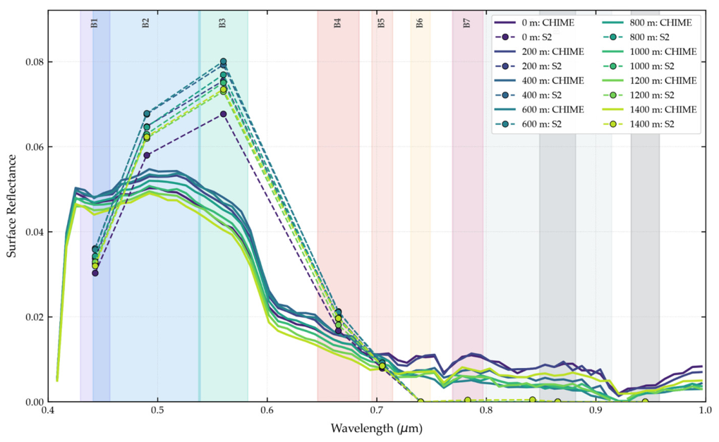
CHIME continuous spectra were able to align with MSI discrete bands in the visible range and correctly capture the strong water absorption in the NIR/SWIR. Along the 1400 m Lago Morto transect on 29 July 2024, atmospherically corrected CHIME and Sentinel-2 L2A data demonstrated strong radiometric alignment (Table 11), with stable RMSE values between 0.0118 and 0.0130 (~1.2%). SAM values, on the other hand, exhibited spatial variation ranging from 17.92° to 22.81°. Deep open-water zones (400–600 m) yielded the highest spectral shape fidelity (SAM ≈ 17.9°), whereas near-shore points (0 m and 1400 m) showed greater divergence (22.81° and 21.00°, respectively). CHIME-Sim spectral signatures show the characteristic shape of moderately turbid water, with a reflectance peak between approximately 0.55–0.57 µm and a sharp decline towards the red and near-infrared wavelengths. Sentinel-2 band values closely follow the CHIME continuum in the visible range (particularly in B2, B3 and B4). While CHIME records a subtle green reflection peak with surface reflectance values ranging between 0.040 and 0.050 across all distance transects (0–1400 m), Sentinel-2 B3 exhibits a significantly higher peak, with values ranging from 0.068 to 0.080. This represents an approximate 40–60% overestimation of green reflectance by Sentinel-2 relative to CHIME. In the near-infrared band (B5–B7), both sensors converge to very low reflectance values (<0.01), consistent with strong water absorption (Figure 13).
Table 11.
Cross-sensor metrics (RMSE and SAM) between atmospherically corrected CHIME and Sentinel-2 L2A surface reflectance along the Lago Morto transect (29 July 2024).
Figure 13.
Spectral signature comparison at the reference location (yellow-circle) between CHIME hyperspectral data surface reflectance—BOA-TOA and Sentinel-02 multispectral bands. Background represents the quantity of bands, and spectral bandwidth of the Sentinel-02 MSI.
In the second Morto Lake pair (Landsat-9 on 19 July versus CHIME on 20 July), spectral signatures extracted at the reference location reveal clear differences between the continuous CHIME hyperspectral curve and the discrete Landsat-9 multispectral samples with a SAM value of 15.12 degrees, an RMSE of 0.0172 and an SS of 0.965 (Figure 14). At the reference location (POI), spectral signatures extracted from CHIME and Landsat-9 reveal clear differences between the continuous hyperspectral curve and the discrete multispectral samples (Figure 14). In the visible range (Landsat bands B1 to B4), both sensors capture a similar overall shape: relatively high reflectance in the blue-green region that declines toward the red. However, the Landsat-9 points show a pronounced peak in B3 (green) that exceeds the CHIME continuum, while B4 (red) sits slightly above the hyperspectral curve. Beyond approximately 0.7 µm the divergence becomes more pronounced. The CHIME signature drops sharply and remains low through the near-infrared, as expected for clear-to-moderately turbid water. In contrast, the Landsat-9 B5 and longer-wavelength bands maintain noticeably higher reflectance values. This NIR offset is consistent with residual atmospheric or adjacency effects that are more pronounced in the broader Landsat bands.
Figure 14.
Spectral signature comparison at the reference location (yellow circle) between CHIME hyperspectral data reflectance-BOA and Landsat-09 multispectral bands. Background represents the quantity of bands, and spectral bandwidth of the Landsat-09 MSI.
These spectral comparisons confirm that the simulated CHIME-Sim data reproduce the essential continuum shape of water reflectance. In the visible range the hyperspectral signatures closely follow the discrete MSI bands, while small systematic offsets (particularly in the green region) are consistent with differences in bandwidth and spectral sampling. In the near-infrared and short-wave infrared both sensors correctly capture the strong absorption by water, with residual divergences attributable to atmospheric residual or adjacency effects that are more pronounced in broader multispectral bands. The ability of CHIME-Sim to resolve finer continuum features while remaining broadly coherent with operational multispectral observations supports its use for pre-launch algorithm testing and for characterizing spectral variability associated with optically active water constituents.
3.1.4. Performance in Narrow and Complex Geometries
The Lambro River represents a particularly challenging environment for the comparison of multispectral and simulated hyperspectral observations because of its narrow and spatially heterogeneous river geometry. The optical analysis was therefore performed exclusively over pixels included within the river water mask, reducing the contribution of surrounding land surfaces and allowing the comparison to focus on the spatial variability of the water signal. Sentinel-2 and simulated CHIME observations were compared using Nechad turbidity, NDCI and NDTI for two coincident acquisitions (22 March and 10 July 2023), with the 22 March acquisition selected as the representative case (Figure 15). The analysis was conceived as a cross-sensor consistency assessment, aimed at determining whether the main spatial anomalies and along-river gradients identified from Sentinel-2 remain recognizable in the corresponding simulated CHIME products, rather than assessing the quantitative equivalence of the retrieved values.
Figure 15.
Spatial comparison of water-quality indicators over the Lambro River on 22 March 2023: (a) Sentinel-2 Nechad turbidity, (b) simulated CHIME Nechad turbidity, (c) Sentinel-2 NDCI, (d) simulated CHIME NDCI, (e) Sentinel-2 NDTI, and (f) simulated CHIME NDTI. The algorithms were applied exclusively to pixels included within the river water mask. Common visualization scales were used for each Sentinel-2–CHIME pair to facilitate the assessment of the preservation of spatial patterns and along-river gradients. DOS-W percentage subtracted: 95% for CHIME images.
The representative comparison shows that spatial variability along the river remains identifiable in the simulated CHIME products, although differences occur in the local magnitude and continuity of the signal. For Nechad turbidity, variations along the river course are visible in both products, with Sentinel-2 providing a more continuous representation of the spatial variability and CHIME showing more localized variations. NDCI and NDTI similarly exhibit differences in their absolute ranges, while spatial changes remain recognizable along corresponding river sections. The comparison is therefore interpreted primarily in terms of the preservation of the relative spatial organization of the signal rather than direct pixel-to-pixel equivalence between the two sensors. Consistency metrics for both acquisitions are reported in Table 12 as complementary descriptors; these metrics are not interpreted as measures of retrieval accuracy, since differences in sensor characteristics, spatial and spectral sampling, and processing can affect the absolute values. High SSIM values (0.95–0.99) confirm that the structural information needed to identify along-river anomalies is retained even under these challenging geometric conditions.
Table 12.
Cross-sensor consistency metrics between Sentinel-2 MSI and simulated CHIME products for Nechad turbidity, NDCI, and NDTI over the Lambro River for the acquisitions of 22 March and 10 July 2023.
Overall, the Lambro analysis provides an initial assessment of the capability of simulated CHIME observations to preserve spatial information relevant to the identification of water anomalies and gradients in a narrow riverine environment. Despite differences in local magnitude and signal continuity, the main along-river variations remain recognizable inside the water mask, and structural similarity remains high. These findings indicate that CHIME-Sim retains diagnostically useful spatial organization even under geometrically challenging conditions, thereby extending the applicability of the simulated products beyond open-water bodies to more complex riverine settings.
3.1.5. Thermal Retrieval Performance of LSTM-Sim
In this study, the quadratic split-window formulation recovers Landsat-referenced surface temperatures with operational accuracy, while the linear model and raw brightness temperature do not, with exemption for one date at Bari. In the Gulf of Taranto, the LSTM-Sim sea-surface temperature retrievals are shown for two dates (Figure 16 and Figure 17). Both the linear (SST-L) and quadratic (SST-Q) formulations successfully recover the principal spatial patterns present in the Landsat 8/9 Band-10 reference, including the cooler offshore waters and the warmer near-shore and embayment zones. However, the linear model exhibits a systematic warm bias, whereas the quadratic model produces temperature magnitudes and spatial gradients that more closely match the Landsat Band 10 level 2 calculations. The statistical evaluation (Table 13) across water pixels highlights the strong performance of the non-linear split-window retrieval. While all three approaches maintain strong spatial agreement with the reference Landsat data (high Pearson correlation coefficients), they differ substantially in absolute calibration. The Raw BT model significantly underestimates surface values due to uncorrected atmospheric attenuation (negative bias of −6.42 to −6.84 °C and RMSE ranging from 6.432 to 6.849 °C). The linear model overcorrects the signal (positive bias of +2.987 to +4.576 °C). The quadratic model successfully addresses these nonlinear atmospheric path effects, achieving superior retrieval accuracy with RMSE ranging from 0.465 to 1.106 °C and relatively low residual bias across both acquisition dates.
Figure 16.
Spatial comparison of water surface temperature (°C) over the Taranto coastal embayment captured on August 06, 2024. From left to right: (a) Landsat 8 Band 10 reference surface temperature; (b) LSTM uncorrected Top-of-Atmosphere Raw Brightness Temperature (10.9 μm); (c) LSTM Linear Split-Window Model (SST-L); and (d) LSTM Quadratic Split-Window Model (SST-Q).
Figure 17.
Spatial comparison of water surface temperature (°C) over the Gulf of Taranto captured on August 14, 2024. From left to right: (a) Landsat 8 Band 10 reference surface temperature; (b) LSTM uncorrected Top-of-Atmosphere Raw Brightness Temperature (10.9 μm); (c) LSTM Linear Split-Window Model (SST-L); and (d) LSTM Quadratic Split-Window Model (SST-Q).
Table 13.
Comparative performance metrics of thermal retrieval models of the Gulf of Taranto Sea Surface Temperature.
In the Gulf of Manfredonia on 28 July 2021, the same pattern is observed (Figure 18, Table 14). Both linear and quadratic formulations recover the principal spatial patterns (warmer near-shore and embayment zones along the western and southern margins, cooler waters farther offshore). The linear model again exhibits a systematic warm bias, while the quadratic model produces temperature magnitudes and spatial gradients that more closely match the Landsat product. The Raw BT model underestimates surface values (bias ≈ −6.216 °C, RMSE ≈ 6.224 °C); the linear model overcorrects (bias ≈ +3.054 °C, RMSE ≈ 3.057 °C); the quadratic model achieves RMSE = 0.275 °C and bias = −0.243 °C.
Figure 18.
Spatial comparison of water surface temperature (°C) over the Gulf of Manfredonia captured on 28 July 2021. From left to right: (a) Landsat-08 Band 10 reference surface temperature; (b) LSTM uncorrected Top-of-Atmosphere Raw Brightness Temperature (10.9 μm); (c) LSTM Linear Split-Window Model (SST-L); and (d) LSTM Quadratic Split-Window Model (SST-Q).
Table 14.
Comparative performance metrics of thermal retrieval models of the Gulf of Manfredonia Sea Surface Temperature.
Along the Coast of Bari three independent dates were examined. On 10 August 2020 (Figure 19, Table 15) both models recover the principal spatial patterns (warmer near-shore waters and cooler offshore gradients). On this date the linear model achieves lower error metrics (RMSE = 1.44 °C, bias = +1.424 °C) than the quadratic model (RMSE = 1.815 °C, bias = –1.804 °C), while Raw BT remains strongly cold-biased. Pearson correlations stay high for all three products. On 27 July 2021 (Figure 20, Table 16) the quadratic model achieves better agreement (RMSE = 0.598 °C, bias = –0.54 °C), while the linear model retains a warm bias of ~2.8 °C and Raw BT retains a cold bias of ~6.5 °C. On 14 September 2021 (Figure 21, Table 17) the quadratic formulation is clearly superior, reducing RMSE from 3.13 °C (linear) and 5.02 °C (Raw BT) to only 0.161 °C, with near-zero bias (0.047 °C). In all the three Coast of Bari cases, the Pearson correlations remain high (>0.90), confirming that spatial structure is preserved regardless of absolute calibration.
Figure 19.
Spatial comparison of water surface temperature (°C) over the Coast of Bari captured on 10 August 2020. From left to right: (a) Landsat-08 Band 10 reference surface temperature; (b) LSTM uncorrected Top-of-Atmosphere Raw Brightness Temperature (10.9 μm); (c) LSTM Linear Split-Window Model (SST-L); and (d) LSTM Quadratic Split-Window Model (SST-Q).
Table 15.
Comparative performance metrics of thermal retrieval models of the Coast of Bari sea surface temperature.
Figure 20.
Spatial comparison of water surface temperature (°C) over the Coast of Bari captured on 28 July 2021. From left to right: (a) Landsat-08 Band 10 reference surface temperature; (b) LSTM uncorrected Top-of-Atmosphere Raw Brightness Temperature (10.9 μm); (c) LSTM Linear Split-Window Model (SST-L); and (d) LSTM Quadratic Split-Window Model (SST-Q).
Table 16.
Comparative performance metrics of thermal retrieval models for sea surface temperature along the Coast of Bari on 28 July 2021.
Figure 21.
Spatial comparison of water surface temperature (°C) over the Coast of Bari captured on 14 September 2021. From left to right: (a) Landsat-08 Band 10 reference surface temperature; (b) LSTM uncorrected Top-of-Atmosphere Raw Brightness Temperature (10.9 μm); (c) LSTM Linear Split-Window Model (SST-L); and (d) LSTM Quadratic Split-Window Model (SST-Q).
Table 17.
Comparative performance metrics of thermal retrieval models for sea surface temperature along the Coast of Bari on 14 September 2021.
Collectively, the thermal results demonstrate that the non-linear (quadratic) split-window correction is essential for operational accuracy in the large majority of cases. Across nearly all examined sites and dates the quadratic model consistently delivers the most accurate surface-temperature retrievals, while the linear model retains a systematic warm bias and the uncorrected brightness temperature remains strongly cold-biased. A single exception is observed at one Bari date, where the linear formulation performs slightly better. High Pearson correlations and SSIM values further confirm that spatial structure is preserved regardless of absolute calibration. These outcomes show that the simulated LSTM thermal products, once appropriately corrected, can recover surface-temperature fields with an accuracy suitable for pre-operational water-quality and discharge-related applications.
3.1.6. Temporal Offsets of Paired Acquisitions for the Virtual-Constellation Concept
To evaluate the temporal relationship between the multispectral and hyperspectral acquisitions used in the pairwise comparison, the time difference between each paired overpass was calculated (Table 18). Of the 15 optical pairs examined, 12 were acquired on the same calendar day. Eleven of these same-day pairs differed by only 2–30 min (median ≈ 11 min), indicating near-simultaneous coverage. Only three pairs showed approximately one-day offsets (≈24.0–24.8 h): Morto Lake (19–20 July 2022), the Gulf of Manfredonia (19–20 January 2021), and Bari coast (23–24 July 2021). These statistics confirm that most of the optical comparisons presented in this study were performed under quasi-synchronous conditions, thereby minimizing the influence of short-term environmental change on the assessment of spatial-pattern consistency. The minority of one-day offsets, already discussed in Section 3.1.2 in relation to hydrological and sediment-dynamics variability, illustrate the residual temporal gaps that can still occur even when selecting the closest available acquisitions.
Table 18.
Time differences between the multispectral and corresponding hyperspectral acquisitions used in the optical results.
Collectively, the acquisition pairs illustrate the practical value of a virtual constellation combining CHIME, with Sentinel-2 and Landsat Multispectral Sensors. Across the six sites, the majority of matchups occur on the same day with temporal offsets of only 2–30 min, while a smaller subset is separated by approximately 24 h; these short intervals quantify the improved temporal sampling that joint observations can provide and confirm that complementary multi-sensor coverage is already achievable for aquatic monitoring.
4. Discussion
Monitoring aquatic ecosystems using satellite remote sensing requires balancing of high spatial, temporal, and spectral resolutions. Inland aquatic environments are highly dynamic, with optical properties influenced by short-term hydrodynamic fluctuations, river discharge variability, and sediment transport. While broad-band multispectral sensors such as Landsat 8/9 have long served as a foundation for regional water-quality assessment, next-generation hyperspectral missions such as CHIME offer the potential for enhanced diagnostic detail through continuous, high-resolution spectral curves. To better separate sensor-driven differences from true environmental change, optical spectral profiles and derived indices (for example, NDTI maps) benefit from evaluation alongside high-frequency hydrological monitoring data. Evaluating how these different sensor architectures characterize optically complex inland and coastal water bodies remains critical for water-quality mapping, constituent retrieval, and index calculation. Consequently, this study examined a paired overpass event between Landsat/Sentinel and CHIME over a different class of water bodies to assess both the technical performance of hyperspectral versus multispectral imagery and the underlying physical dynamics of the site.
Spectral signatures form the foundation of optical remote sensing for aquatic monitoring, as constituents such as chlorophyll-a, suspended solids, and coloured dissolved organic matter can influence absorption and reflectance across the visible and near-infrared spectrum [62]. Multispectral platforms such as Landsat 8/9 and Sentinel-2 offer spatial advantages, particularly for capturing localized features. Sentinel-2’s native 10 m spatial resolution can reduce geometric and pixel-mixing uncertainties, supporting the delineation of narrow plumes and fine shoreline features. However, the broad and discrete spectral bands of multispectral sensors limit the characterization of detailed spectral variability. CHIME is expected to complement these observations by providing contiguous narrow-band measurements that can resolve spectral features not adequately represented by multispectral bands, particularly across the visible spectrum. In the present study, this capability is evaluated in terms of spectral-signature characterization and comparison with multispectral observations; the identification of specific contaminants is not directly assessed.
To evaluate shape alignment between continuous hyperspectral curves and discrete multispectral bands, the SAM measures vector orientation in n-dimensional space. Because surface water exhibits low absolute reflectance, localized band discrepancies, such as green-band atmospheric residuals or adjacency effects, disproportionately rotate the spectral vector relative to strongly absorbing NIR and SWIR channels. Consequently, acceptable SAM thresholds for aquatic targets are broader than traditional terrestrial standards. In inland and coastal-lagoon water spectroscopy, cosine similarity scores of ≥0.80 (corresponding to SAM angles ≤ 0.64 rad/~37°) are accepted as the baseline for relative spectral shape agreement, while scores ≥0.90 (SAM angles ≤ 0.45 rad/~26°) are recognized as strong indicators of spectral shape fidelity [49,50], confirming that discrete multispectral samples can effectively preserve the overarching spectral continuum defined by hyperspectral measurements despite minor radiometric offsets.
This complementarity suggests a division of roles in which multispectral imagery supports the spatial delineation of localized water-quality patterns, while hyperspectral observations provide more detailed characterization of their spectral variability. An analogous advantage of contiguous hyperspectral measurements was reported by Valentini et al. [63], although that study concerned topsoil applications. In the present study, the potential contribution of hyperspectral observations is illustrated by the ability of CHIME-Sim to represent continuous water-reflectance signatures and resolve spectral variations that are only sparsely sampled by Sentinel-2 and Landsat bands. In the Gulf of Manfredonia and Morto Lake cases, the simulated and operational products preserved comparable dominant spatial gradients despite temporal and sensor-related differences. These findings support a two-tiered framework in which multispectral imagery contributes to the spatial detection and delineation of potential water-quality anomalies, while hyperspectral observations provide additional spectral information for their characterization. However, the present analysis does not identify specific contaminants, determine discharge composition, or attribute observed patterns to individual sources. Such interpretations would require independent information, including synchronous in situ water-quality measurements, laboratory or field spectral characterization, and contextual evidence on potential discharge sources.
Accordingly, contaminant identification and source attribution are considered potential future applications of CHIME observations when combined with suitable in situ and ancillary information, rather than capabilities demonstrated by the present study.
Alongside advancements in optical sensing, the Copernicus LSTM mission aims to address the long-standing spatio-temporal trade-off in thermal infrared (TIR) remote sensing by delivering 50-m field-scale imagery with a 1-to-3-day revisit frequency. Existing operational thermal sensors generally require users to choose between high spatial resolution with long revisit intervals (Landsat) or coarse spatial resolution with daily coverage (MODIS or Sentinel-3). By incorporating five dedicated TIR channels, LSTM enables simultaneous high-precision retrieval of surface emissivity and land-surface temperature [64]. It specifically targets the high-frequency gap that Landsat cannot fully fill, while planning future synergies with Landsat Next, TRISHNA, and SBG [62,65]. The comparative performance of the LSTM-Sim data for sea-surface temperature retrievals in this study indicates that atmospheric path effects over coastal waters are highly non-linear. Uncorrected brightness temperatures tend to underestimate surface values, while standard linear split-window models using MODIS constants can substantially overcorrect the signal. Therefore, future thermal monitoring missions in coastal environments would benefit from prioritizing practical quadratic split-window algorithms to better account for complex atmospheric water-vapor absorption and improve absolute calibration, a reality previously addressed by Du et al. [59].
Atmospheric water vapor significantly attenuates thermal infrared radiation because water vapor molecules absorb surface-emitted radiance and re-emit it at cooler atmospheric temperatures, leading to a reduction in the brightness temperatures detected by the sensor. Because this absorption is wavelength-dependent, atmospheric transmittance is lower and atmospheric radiation is higher in a thermal band of ~12 µm than in a thermal band of ~10 µm, which means atmospheric attenuation by water vapor is itself non-linear. Split-window algorithms exploit this differential attenuation between the two thermal channels to quantify and correct for the atmospheric effect [65]. This superior performance of the quadratic (non-linear) split-window formulation relative to the linear model is consistent with well establish theory and Landsat-08/09 applications, in which the inclusion of quadratic terms of the brightness-temperature differentiates effectively, and compensates for residual nonlinear atmospheric attenuation, with values in coastal waters typically with an RMSE < 1 °C and near-zero bias over coastal waters [66].
The integration of these emerging missions, such as CHIME and LSTM, with observations from existing MSI satellites within a virtual constellation indicates new opportunities for improving the monitoring of water dynamics. Remote sensing in riverine environments faces several physical constraints, such as mixed pixels in narrow channels, atmospheric cloud cover during critical flood events, and empirical ground calibrations that change during high-discharge conditions [62]. However, combining observations from different satellite sensors offers a cost-effective, non-invasive alternative that substantially improves temporal frequency [67]. For example, CilleroCastro et al. [68] demonstrated that integrating Sentinel-2 and Landsat-8 reduced the effective revisit time to around 5 days, and more recent estimates place this virtual constellation’s revisit time at approximately 2.9 days [69]. By embedding these long-term constellations into advanced frameworks, such as spatiotemporal deep-learning models, standard limitations, such as the inability to differentiate specific algal groups in the Moselle River due to restricted spectral bands, may progressively be reduced [70,71]. In this study, the cross-sensor intervals observed across the study sites further support the operational potential of a CHIME–MSI virtual constellation. By reducing effective revisit gaps to minutes or, at most, roughly one day, the combined observations offer a practical means of capturing rapid shifts in water composition and transient anomalies that would otherwise be missed by any single sensor, thereby helping to overcome the well-known constraints of these environments. Nevertheless, additional studies spanning longer time series and a wider range of aquatic conditions will be required to fully quantify these benefits and to validate the approach under operational settings.
Within this multisensor framework, the comparison between simulated CHIME observations and currently operational multispectral sensors was primarily conceived as a cross-sensor consistency assessment. Rather than seeking quantitative equivalence between retrieved values, the analysis evaluated whether the main spatial patterns, localized anomalies, and spatial gradients identified in the multispectral observations remained recognizable in the corresponding simulated CHIME products. This approach was particularly relevant for the Lambro River, where the narrow and heterogeneous river geometry makes direct pixel-level comparisons sensitive to differences in spatial sampling. Despite differences in absolute values and local spatial continuity, the comparison indicated that relevant elements of the spatial organization observed by Sentinel-2 remained identifiable in the simulated CHIME products. The statistical metrics were therefore used as complementary descriptors of cross-sensor consistency, while the interpretation focused primarily on the preservation of spatial information rather than retrieval accuracy.
Despite these operational advantages, several technical and methodological limitations must be considered. A critical factor in this study is the process used to convert TOA radiance to TOA reflectance for the CHIME-Sim products, which relied on the TSIS-1 Hybrid Solar Reference Spectrum (HSRS). While this spectrum is highly accurate, differences between solar irradiance models can reach several percent in the ultraviolet and near-infrared regions [37,72]. These residual discrepancies may propagate into the derived TOA reflectance, particularly in the blue and SWIR bands, becoming relevant when comparing absolute reflectance values with independent datasets. Furthermore, a full atmospheric correction to water-leaving reflectance was not applied due to the lack of mission-specific auxiliary information for the pre-operational products. This limitation caused elevated SWIR baselines in the Morto Lake turbidity map, likely due to uncorrected skylight glint or aerosol scattering often occurring when the dark-pixel assumption is violated in turbid waters [73].
Finally, the limited availability of in situ data remains an important constraint for the calibration and validation of remote-sensing products. Conventional field monitoring is often restricted in spatial coverage, frequency, and representativeness, which limits the independent validation of remote-sensing estimates under different environmental conditions. This is particularly relevant for inland waters, where highly variable optical properties make the transferability of remote-sensing algorithms between different water bodies challenging [74,75,76]. To overcome these spatial limitations and improve the reliability of derived products, future work will focus on expanding validation through airborne campaigns and synchronous in situ field match-ups across diverse optical water types. Additionally, efforts will center on developing dedicated atmospheric correction algorithms to address SWIR glint and non-linear thermal attenuation over dark aquatic targets and integrating these future hyperspectral sensors with existing multispectral into a high-frequency virtual constellation and embedding continuous hyperspectral unmixing and thermal products into operational data-assimilation and early-warning workflows for dynamic water monitoring.
The complementarity observed between optical and thermal information should not be interpreted as a quantitative demonstration that their combination improves anomaly-detection performance. The present experiments were designed primarily to assess cross-sensor consistency and the suitability of simulated CHIME and LSTM products for future multisensor applications. Demonstrating an actual detection gain would require a dedicated experimental design in which anomaly-detection performance obtained from optical-only, thermal-only, and combined optical–thermal configurations is evaluated against independent reference observations or documented events.
Nevertheless, establishing consistent and complementary information across the considered sensors represents an important prerequisite for developing such integrated approaches and supports the investigation of optical–thermal fusion once observations from the future missions become available.
Similarly, the detailed spectral information provided by CHIME-Sim should not be interpreted as direct evidence of contaminant identification or source attribution. The present analysis evaluates spectral signatures, turbidity-related products, and spatial patterns but does not include the independent chemical measurements or validated spectral libraries required to associate individual spectral features with specific contaminants. The results therefore demonstrate enhanced spectral characterization rather than definitive compositional identification.
Future work will focus on: (i) developing dedicated atmospheric correction algorithms to address SWIR glint and non-linear thermal attenuation over dark aquatic targets; (ii) expanding validation through airborne campaigns and synchronous in situ match-ups across diverse optical water types; (iii) integrating CHIME, LSTM, and existing multispectral sensors into a high-frequency virtual constellation; and (iv) embedding continuous hyperspectral unmixing and thermal products into operational data assimilation and early-warning workflows for dynamic water monitoring.
5. Limitations
The results support the potential joint exploitation of optical and thermal observations for future aquatic anomaly-detection applications by demonstrating the cross-sensor consistency and complementarity required for multisensor analysis. However, the present study does not quantify the improvement in anomaly-detection performance resulting from their combined use. Establishing such a benefit would require dedicated comparisons between single-sensor and multisensor detection approaches using independent reference information.
The cross-sensor comparisons performed in this study were conceived primarily as a consistency assessment between simulated CHIME observations and currently operational multispectral sensors. Rather than seeking quantitative equivalence between the retrieved values, the analysis focused on whether the main spatial patterns, localized anomalies, and spatial gradients identified in the multispectral observations remained recognizable in the corresponding simulated CHIME products. This aspect is particularly relevant for the Lambro River, where the narrow geometry of the water body makes direct pixel-level comparisons especially sensitive to differences in spatial sampling. The results indicate that, despite differences in absolute values and local spatial continuity, the simulated CHIME products preserve relevant elements of the spatial organization observed in the Sentinel-2 products. The statistical metrics were therefore used as complementary descriptors of cross-sensor consistency, while the interpretation focused primarily on the preservation of spatial information rather than on retrieval accuracy.
Although the simulated CHIME and LSTM datasets used in this study effectively demonstrate the potential of these upcoming missions, they remain limited by the properties of the sensors from which they were derived. CHIME simulations are currently generated from data acquired by existing instruments such as PRISMA, EnMAP, and HySpex. As a result, the spectral coverage of the simulated products is constrained by the wavelength ranges of these precursor sensors, making it impossible to reconstruct CHIME bands beyond those domains [8]. Similarly, because the LSTM data evaluated in this study were simulated directly from Landsat observations, the potential temporal synergy associated with different acquisition times for monitoring of dynamic water events could not be fully assessed. Nevertheless, these simulation approaches remain highly valuable; they demonstrate a spatial fidelity consistent with the higher resolution of the expected products and support meaningful baseline comparisons with existing sensors such as Landsat 8/9 OLI, but attention needs to be put in the coefficient used according to the site of study.
A more critical limitation lies in the current data processing workflow, particularly regarding atmospheric correction. The atmospheric correction applied to the simulated datasets is a simplified version not specifically developed for complex aquatic environments. For instance, the Dark Object Subtraction (DOS-NIR) approach is prone to failure in turbid waters, as the strong backscattering generated by suspended matter can be erroneously misinterpreted as atmospheric aerosol. Therefore, the development of accurate, water-specific atmospheric correction methods for CHIME imagery, particularly to address elevated baselines in the SWIR bands, warrants dedicated attention. Fortunately, the recent deployment of operational hyperspectral satellites, such as PRISMA and EnMAP, has accelerated the development of advanced atmospheric correction algorithms adapted for aquatic applications (SeaDAS, POLYMER, and iCOR), facilitating a broader evaluation of different radiative transfer approaches.
Finally, the lack of sufficient in situ data restricts the independent validation of these remote-sensing estimates. While satellite imagery provides essential, large-scale spatial coverage, in situ observations supply the fundamental ground truth required to verify what is physically occurring within the water column. Securing synchronous match-ups between future satellite overpasses and active measurement sites is essential. Expanding these field datasets will allow for more robust statistical analyses and provide deeper insights into sensor performance across varying observation geometries, atmospheric conditions, and diverse optical water types.
A further limitation concerns the interpretation of the hyperspectral signatures. Although CHIME-Sim provides substantially denser spectral sampling than Sentinel-2 and Landsat, the present study does not include chemical analyses, validated contaminant-specific spectral endmembers, or independent source information. Consequently, the observed spectral variability cannot be attributed unambiguously to specific contaminants or discharge sources. The hyperspectral results are therefore interpreted as evidence of enhanced spectral characterization and potential discrimination of optically distinct water conditions rather than as direct identification of contaminant composition or source.
6. Conclusions
This study assessed the use of simulated CHIME and LSTM observations in combination with currently available Sentinel-2 and Landsat products as a preparatory step toward future multisensor monitoring of inland and coastal waters. The results show that the simulated products reproduce relevant spatial and spectral or thermal patterns observed in operational satellite products while also providing complementary information associated with the expected characteristics of the future missions. CHIME-Sim provides continuous hyperspectral information that supports a more detailed characterization of spectral variability in water bodies, whereas LSTM-Sim provides complementary thermal information for characterizing surface-temperature patterns.
The analyses should primarily be interpreted as a cross-sensor assessment of simulated future-mission products rather than as a demonstration of the full performance of a CHIME-LSTM-Sentinel-2-Landsat virtual constellation. In particular, the present study does not quantify an improvement in anomaly-detection performance resulting from the combined use of optical and thermal observations, nor does it demonstrate the identification of specific contaminants or attribution of observed anomalies to individual discharge sources. Similarly, agreement with operational satellite products should not be interpreted as independent validation of absolute retrieval accuracy where the reference observations themselves are remotely sensed products or are related to the data used in the simulation chain.
Nevertheless, the observed cross-sensor consistency supports the use of simulated CHIME and LSTM datasets for the development and testing of processing chains before the missions become operational. Their future integration with Sentinel-2 and Landsat offers the prospect of exploiting complementary hyperspectral, multispectral, and thermal observations within a common aquatic-monitoring framework. Future work should assess the added value of this joint exploitation quantitatively, including its effect on temporal observation opportunities and anomaly-detection performance, and should incorporate independent in situ measurements where required for the validation of absolute water-quality and surface-temperature products.
Author Contributions
Conceptualization, J.A.V.-S., V.S., A.A. and G.C.; methodology, J.A.V.-S., V.S., A.A. and G.C.; software J.A.V.-S. and V.S.; validation, P.K. and M.K.; data curation, P.D.L. and J.A.V.-S.; writing—original draft preparation J.A.V.-S. and V.S.; writing—review and editing, M.K., P.K., V.K., A.A., G.C., P.D.L., J.A.V.-S. and E.L.; visualization, P.K. and M.K.; supervision, M.K., V.K., A.A., G.C. and E.L.; project administration, A.A.; funding acquisition, G.C. All authors have read and agreed to the published version of the manuscript.
Funding
This work was supported by the Sentinel Users Preparation (SUP) initiative of the European Space Agency under ESA Contract No. 4000146580/24/I-DT-bgh (Multisensor Water Discharges Project).
Data Availability Statement
The simulated CHIME and simulated LSTM datasets are available from the APEX/ESA for the MWD project repository at the following links: CHIME-Sim: https://browser.apex.esa.int/external/eoresults.esa.int/stac/collections/mwd-chime-sim?.language=en; LSTM-Sim: https://browser.apex.esa.int/external/eoresults.esa.int/stac/collections/mwd-lstm-sim. The Sentinel-2 data are available from the public repository “Copernicus Data Space Ecosystem” at https://dataspace.copernicus.eu (accessed on 12 September 2026), and the Landsat 8/9 datasets are available from the public repository “USGS Earth Explorer” at https://earthexplorer.usgs.gov (accessed on 12 September 2026). The solar irradiance TSIS-1 HSRS data are available at https://lasp.colorado.edu/lisird/data/tsis1_hsrs (accessed on 12 September 2026). The dataset used in this study corresponds specifically to the TSIS-1 HSRS 1 nm data from this data center. Any other datasets or code generated and/or analyzed during the current study are available from the corresponding author upon reasonable request.
Conflicts of Interest
Authors Antonello Aiello, Giulio Ceriola, Paola Di Lauro and Valentina Santarsiero were employed by the company Planetek. The remaining authors declare that the research was conducted in the absence of any commercial or financial relationships that could be construed as a potential conflict of interest.
Abbreviations
The following abbreviations are used in this manuscript:
| ASI | Italian Space Agency |
| BOA | Bottom-of-Atmosphere |
| BPC | Biopolymeric Carbon |
| DSF | Dark Spectrum Fitting |
| Cd | Cadmium |
| CDOM | Color Dissolved Organic Matter |
| CHIME | Copernicus Hyperspectral Imaging Mission for the Environment |
| Chl-a | Chlorophyll-a |
| Cr | Cromium |
| CRS | Coordinated Reference System |
| Cu | Copper |
| DN | Digital Number |
| ECMWF | European Centre for Medium-Range Weather Forecasts |
| EO | Earth Observation |
| ERA5 | ECMWF Reanalysis v5 |
| ESA | European Space Agency |
| GEE | Google Earth Engine |
| GEOGLOWS | Group on Earth Observations Global Water Sustainability |
| GSD | Ground Sample Distance |
| Hg | Mercury |
| HSI | HyperSpectral Imager |
| HRSR | Hybrid Solar Reference Spectrum |
| IFS | Integrated Forecasting System |
| LSTM | Land Surface Temperature Monitoring |
| LS8 | Landsat-08 |
| LS9 | Landsat-09 |
| MERIS | Medium Resolution Imaging Spectrometer |
| MNDWI | Modified Normalized Difference Water Index |
| MODIS | Moderate Resolution Imaging Spectroradiometer |
| MSI | Multispectral Imaginer |
| MWD | Multisensor Water Discharges |
| NASA | National Aeronautics and Space Administration |
| NDTI | Normalized Difference Turbidity Index |
| NDWI | Normalized Difference Water Index |
| NIR | Near Infrared |
| OLCI | Ocean and Land Colour Instrument |
| OLI | Operational Land Imager |
| PAHs | Polycyclic Aromatic Hydrocarbons |
| Pb | Lead |
| PCBs | Polychlorinated Biphenyls |
| PRISMA | Hyperspectral Precursor of the Application Mission |
| RFS | River Forecast System |
| RMSE | Root Mean Square Error |
| S2 | Sentinel-02 |
| SABI | Superficial Algae Bloom Index |
| SAM | Spectral Angle Mapper |
| SeaWiFS | Sea-Viewing Wide Field-of-View Sensor |
| SIM | Structure Similarity Index Measure |
| SLSTR | Sea and Land Surface Temperature Radiometer |
| SS | Spectral Similarity Score |
| SWIR | Short-Wave Infrared |
| TDX-Hydro | TanDEM-X-derived hydrography |
| TIR | Thermal Infrared |
| TIRS | Thermal Infrared Sensor |
| TOA | Top-of-Atmosphere |
| TOC | Total Organic Carbon |
| TSIS-1 | Total and Spectral Solar Irradiance Sensor-1 |
| USGS | United States Geological Survey |
| UTM | Universal Transverse Mercator |
| VIIRS | Visible Infrared Imaging Radiometer Suite |
| VIS | Visible |
| VNIR | Visible-Near Infrared |
| VSWIR | Visible Shortwave Infrared |
| WBCI | Water Body Chlorophyll Index |
| Zn | Zinc |
Appendix A. Summary of Satellite Data (Multispectral)
This first appendix provides a comprehensive summary of the satellite and airborne datasets utilized in this study. The candidate data was selected from a broader repository of available imagery based on their spatial coverage of the selected study areas between 2019 and early 2025. To ensure data quality, acquisitions were filtered to include only those with cloud cover of less than 60%. From all the available images, and considering the workflow proposed in this study, only MSI images that could be used in conjunction with hyperspectral satellite data were considered, namely CHIME or LSTM-simulated data.
Table A1.
Multispectral image data acquisitions (Sentinel or Landsat satellites).
Table A2.
Hyperspectral image data acquisitions (CHIME and LSTM sim data).
Appendix B
To convert Top-of-Atmosphere (TOA) radiance (LTOA) to TOA reflectance (ρTOA), precise band-averaged extraterrestrial solar irradiance (F0) values are required. These parameters were derived by convolving the high-resolution solar irradiance spectrum (TSIS-1 Hybrid Solar Reference Spectrum) with the specific relative spectral response functions of the sensor, characterized by each band’s center wavelength and Full Width at Half Maximum (FWHM). The following table details the calculated mean extraterrestrial solar irradiance (F0) and its associated uncertainty () across the spectral bands (B1–B240) used in the normalization workflow for the CHIME-Sim radiance.
Table A3.
Extraterrestrial solar irradiance (F0) values per band.
References
- Gholizadeh, M.H.; Melesse, A.M.; Reddi, L.; Gholizadeh, M.H.; Melesse, A.M.; Reddi, L. A comprehensive review on water quality parameters estimation using remote sensing techniques. Sensors 2016, 16, 1298. [Google Scholar] [CrossRef] [Scilit] [PubMed]
- Copernicus Sentinel Expansions Missions. Available online: https://www.esa.int/Applications/Observing_the_Earth/Copernicus/Copernicus_Sentinel_Expansion_missions (accessed on 8 September 2026).
- Garro, L.; Sorriso, A.; Gamba, P.; Sosmanidis, P.; Keramitsoglou, I.; Kiranoudis, C.T.; Fischer, J. Simulating and Validating CHIME and LSTM Data for Urban Material Characterization. Remote Sens. 2026, 18, 442. [Google Scholar] [CrossRef] [Scilit]
- Nieke, J.; Despoisse, L.; Gabriele, A.; Weber, H.; Strese, H.; Ghasemi, N.; Gascon, F.; Alonso, K.; Boccia, V.; Tsonevska, B.; et al. The Copernicus Hyperspectral Imaging Mission for the Environment (CHIME): An Overview of Its Mission, System and Planning Status. Sens. Syst. Next-Gener. Satell. XXVII 2023, 12729, 21–40. [Google Scholar] [CrossRef] [Scilit]
- Rast, M.; Adams, J.; Gascon, F.; Nieke, J.; Ananasso, C.; Bach, H.; Dor, B.; Chabrillat, S.; Colombo, R.; Feret, J.-B.; et al. ESA UNCLASSIFIED-for Official Use Title Copernicus Hyperspectral Imaging Mission for the Environment-Mission Requirements Document Issue Number 3 Revision Number 0; European Space Agency (ESA): Noordwijk, The Netherlands, 2021. [Google Scholar]
- Candiani, G.; Tagliabue, G.; Panigada, C.; Verrelst, J.; Picchi, V.; Rivera Caicedo, J.P.; Boschetti, M. Evaluation of Hybrid Models to Estimate Chlorophyll and Nitrogen Content of Maize Crops in the Framework of the Future CHIME Mission. Remote Sens. 2022, 14, 1792. [Google Scholar] [CrossRef] [Scilit] [PubMed]
- Segl, K.; Guanter, L.; Gascon, F.; Kuester, T.; Rogass, C.; Mielke, C. S2eteS: An End-to-End Modeling Tool for the Simulation of Sentinel-2 Image Products. IEEE Trans. Geosci. Remote Sens. 2015, 53, 5560–5571. [Google Scholar] [CrossRef] [Scilit]
- Koutsantoni, P.; Kremezi, M.; Karathanassi, V.; Di Lauro, P.; Vargas-Solano, J.A.; Ceriola, G.; Aiello, A.; Lamboglia, E. A Multisensor Framework for Satellite Data Simulation: Generating Representative Datasets for Future ESA Missions—CHIME and LSTM. Remote Sens. 2026, 18, 1384. [Google Scholar] [CrossRef] [Scilit]
- Cavalli, R.M. Comparison of Split Window Algorithms for Retrieving Measurements of Sea Surface Temperature from MODIS Data in Near-Land Coastal Waters. ISPRS Int. J. Geo-Inf. 2018, 7, 30. [Google Scholar] [CrossRef] [Scilit]
- Mali, M.; Dell’anna, M.M.; Mastrorilli, P.; Damiani, L.; Ungaro, N.; Gredilla, A.; de Vallejuelo, S.F.-O. Identification of hot spots within harbour sediments through a new cumulative hazard index. Case study: Port of Bari, Italy. Ecol. Indic. 2016, 60, 548–556. [Google Scholar] [CrossRef] [Scilit]
- Magni, S.; Nigro, L.; Della-Torre, C.; Binelli, A. Characterization of plastics and their ecotoxicological effects in the Lambro River (N. Italy). J. Hazard. Mater. 2021, 412, 125204. [Google Scholar] [CrossRef] [Scilit] [PubMed]
- Zanetti, M.; Piccolo, D.; Bellio, M.; Turin, P.; Floris, B.; Russino, G.; Zanetti, M.; Piccolo, D.; Bellio, M.; Turin, P.; et al. Indagine sulla fauna ittica del lago di Cadore (Belluno): Prove di genotossicità e bioaccumolo dei metalli pesanti. J. Freshw. Biol. 2006, 34, 351–358. [Google Scholar]
- Dei Cont, L. Caratterizzazione idrogeologica della sorgente del Meschio in Savassa Alta, Vittorio Veneto, TV. Master’s Thesis, University of Padua, Padua, Italy, 2020/2021. [Google Scholar]
- Bettineti, R.; Giarei, C.; Provini, A. Chemical Analysis and Sediment Toxicity Bioassays to Assess the Contamination of the River Lambro (Northern Italy). Arch. Environ. Contam. Toxicol. 2003, 45, 72–78. [Google Scholar] [CrossRef] [Scilit] [PubMed]
- Viganò, L.; Loizezau, J.L.; Mandich, A.; Mascolo, G. Medium-and long-term effects of estrogenic contaminants on the middle river Po fish community as reconstructed sediment core. Arch. Environ. Contam. Toxicol. 2016, 71, 454–472. [Google Scholar] [CrossRef] [Scilit] [PubMed]
- Marziali, L.; Valsecchi, L.; Schiavon, A.; Mastroianni, D.; Viganò, L. Vertical profiles of trace elements in a sediment core from the Lambro River (northern Italy): Historical trends and pollutant transport to the Adriatic Sea. Sci. Total Environ. 2021, 782, 146766. [Google Scholar] [CrossRef] [Scilit] [PubMed]
- Rizzo, D.; Pontin, A.; Fullin, N.; Piccinini, L. A Hybrid Stochastic Numerical Framework for Predictive Groundwater Risk Mapping: Integrating Time-Dependent Scenarios in a Strategic Alpine Aquifer. Sustainability 2026, 18, 4412. [Google Scholar] [CrossRef] [Scilit]
- Babagolimatikolaei, J. Effecto of variations in po river discharge on physical water characeristics and chlorophyll-a levels in the gulf of Manfredonia. Geosci. Lett. 2024, 11, 24. [Google Scholar] [CrossRef] [Scilit]
- Rizzo, A.; Scicchitano, G.; Mastronuzzi, G.A. A set of guidelines as support for the integrated geo-environmental characterization of highly contaminated coastal sites. Sci. Rep. 2024, 14, 8198. [Google Scholar] [CrossRef] [Scilit] [PubMed]
- Fossile, E.; Sabbatini, A.; Spagnoli, F.; Caridi, F.; Dell’Anno, A.; De Marco, R.; Dinelli, E.; Droghini, E.; Tramontana, M.; Negri, A. Sensitivity of foraminiferal-based indices to evaluate the ecological quality status of marine coastal benthic systems: A case study of the Gulf of Manfredonia (southern Adriatic Sea). Mar. Pollut. Bull. 2021, 163, 111933. [Google Scholar] [CrossRef] [Scilit] [PubMed]
- Cecere, E.; Petrocelli, A.; Belmonte, M.; Portacci, G.; Rubino, F. Activities and vectors responsible for the biological pollution in the Taranto Seas (Mediterranean Sea, southern Italy): A review. Environ. Sci. Pollut. Res. 2016, 23, 12797–12810. [Google Scholar] [CrossRef] [Scilit] [PubMed]
- De Serio, F.; Mossa, M. Environmental monitoring in the Mar Grande basin (Ionian Sea, Southern Italy). Environ. Sci. Pollut. Res. 2016, 23, 12662–12674. [Google Scholar] [CrossRef] [Scilit] [PubMed]
- Petrelli, V.; Ferraro, A.; Fratino, U.; Mali, M.; Spasiano, D.; Dell’Anna, M.M. Microplastic pollution in Italian South Adriatic Harbor Areas. In Proceedings of the IEEE International Workshop on Metrology for the Sea; Learning to Measure Sea Health Parameters (MetroSea), La Valletta, Malta, 4–6 October 2023; pp. 269–273. [Google Scholar] [CrossRef] [Scilit]
- Mali, M.; Dell’Anna, M.M.; Mastrorilli, P.; Damiani, L.; Ungaro, N.; Belviso, C.; Fiore, S. Are conventional statistical techniques exhaustive for defining metal background concentrations in harbour sediments? A case study: The Coastal Area of Bari (Southeast Italy). Chemosphere 2015, 138, 708–717. [Google Scholar] [CrossRef] [Scilit] [PubMed]
- Renzi, M.; Perra, G.; Guerranti, C.; Mariotinni, M.; Baroni, D.; Volterrani, M.; Graziosi, M. Assessment of environmental pollutants in ten southern Italy harbor sediments. Toxicol. Ind. Health 2009, 25, 351–363. [Google Scholar] [CrossRef] [Scilit] [PubMed]
- Magoffin, R.H.; Hales, R.C.; Nelson, E.J.; Wara, C.; Williams, G.P.; South, A.; Challa, Z.K. Hydrologic Decision Support in the Nile Basin: Creating Status Products from the GEOGLOWS Hydrologic Model. Hydrology 2025, 12, 43. [Google Scholar] [CrossRef] [Scilit]
- Hales, R.C.; Nelson, E.J.; Souffront, M.; Gutierrez, A.L.; Prudhomme, C.; Kopp, S.; Ames, D.P.; Williams, G.P.; Jones, N.L. Advancing Global Hydrologic Modeling with the GEOGloWS ECMWF Streamflow Service. J. Flood Risk Manag. 2025, 18, e12859. [Google Scholar] [CrossRef] [Scilit]
- Sagan, V.; Peterson, K.T.; Maimaitijiang, M.; Sidlike, P.; Sloan, J.; Greenling, B.A.; Maalouf, S.; Adams, C. Monitoring inland water quality using remote sensing: Potential and limitations of spectral indices, bio-optical simulations, machine learning, and cloud computing. Earth-Sci. Rev. 2020, 205, 103187. [Google Scholar] [CrossRef] [Scilit]
- Xu, H.Q. Modification of normalized difference water index (NDWI) to enhance open water features in remotely sensed imagery. Int. J. Remote Sens. 2006, 27, 3025–3033. [Google Scholar] [CrossRef] [Scilit]
- Lacaux, J.P.; Tourre, Y.M.; Vignolles, C.; Ndione, J.A.; Lafaye, M. Classification of ponds from high-spatial resolution remote sensing: Application to Rift Vallet Fever epidemics in Senegal. Remote Sens. 2007, 106, 66–74. [Google Scholar] [CrossRef] [Scilit]
- Pan, X.; Yuan, J.; Yang, Z.; Tansey, K.; Xie, W.; Song, H.; Wu, Y.; Yang, Y. Spatio-Temporal Variation of Cyanobacteria Blooms in Taihu Lake Using Multiple Remote Sensing Indices and Machine Learning. Remote Sens. 2024, 16, 889. [Google Scholar] [CrossRef] [Scilit]
- Barraza-Moraga, F.; Alcayaga, H.; Pizzaro, A.; Félez-Bernal, J.; Urrutia, R.; Barraza-Moraga, F.; Alcayaga, H.; Pizarro, A.; Félez-Bernal, J.; Urrutia, R. Estimation of chlorophyll-a concentrations in Lanalhue Lake using Sentinel-2 MSI satellite images. Remote Sens. 2022, 14, 5647. [Google Scholar] [CrossRef] [Scilit]
- Du, Y.; Zhang, Y.; Ling, F.; Wang, Q.; Li, W.; Li, X. Water Bodies Mapping from Sentinel-2 Imagery with Modified Normalized Difference Water Index at 10-m Spatial Resolution Produced by Sharpening the SWIR Band. Remote Sens. 2016, 8, 354. [Google Scholar] [CrossRef] [Scilit]
- Clerc, S.; Rodat, D.; Lafrance, B.; Alhammoud, B.; Enache, S.; Deru, A.; Rivoire, L.; Adriaensen, S.; Hillairet, E.; Morrone, R.; et al. Copernicus Sentinel-2C Radiometric Calibration and Validation Status. Remote Sens. 2026, 18, 1387. [Google Scholar] [CrossRef] [Scilit]
- Alparone, L.; Garzelli, A. Downscaling Land Surface Temperature via Assimilation of LandSat 8/9 OLI and TIRS Data and Hypersharpening. Remote Sens. 2024, 16, 4694. [Google Scholar] [CrossRef] [Scilit]
- Kwong, I.H.Y.; Wong, F.K.K.; Fung, T. Automatic Mapping and Monitoring of Marine Water Quality Parameters in Hong Kong Using Sentinel-2 Image Time-Series and Google Earth Engine Cloud Computing. Front. Mar. Sci. 2022, 9, 871470. [Google Scholar] [CrossRef] [Scilit]
- Coddington, O.M.; Richard, E.C.; Harber, D.; Pilewskie, P.; Woods, T.N.; Chance, K.; Liu, X. The TSIS-1 Hybrid Solar Reference Spectrum. Geophys. Res. Lett. 2021, 48, e2020GL091709. [Google Scholar] [CrossRef] [Scilit] [PubMed]
- Giardino, C.; Bresciani, M.; Braga, F.; Fabbretto, A.; Ghirardi, N.; Pepe, M.; Gianinetto, M.; Colombo, R.; Cogliati, S.; Ghebrehiwot, S.; et al. First Evaluation of PRISMA Level 1 Data for Water Applications. Sensors 2020, 20, 4553. [Google Scholar] [CrossRef] [Scilit] [PubMed]
- Guanter, L.; Kaufmann, H.; Segl, K.; Foerster, S.; Rogass, C.; Chabrillat, S.; Kuester, T.; Hollstein, A.; Rossner, G.; Chlebek, C.; et al. The EnMAP Spaceborne Imaging Spectroscopy Mission for Earth Observation. Remote Sens. 2015, 7, 8830–8857. [Google Scholar] [CrossRef] [Scilit]
- Chavez, P.S., Jr. An improved dark-object subtraction technique for atmospheric scattering correction of multispectral data. Remote Sens. Environ. 1988, 24, 459–479. [Google Scholar] [CrossRef] [Scilit]
- Sobrino, J.A.; Jiménez-Muñoz, J.C.; Paolini, L. Land surface temperature retrieval from LANDSAT TM 5. Remote Sens. Environ. 2004, 90, 434–440. [Google Scholar] [CrossRef] [Scilit]
- Pan, Y.; Bélanger, S.; Huot, Y. Evaluation of Atmospheric Correction Algorithms over Lakes for High-Resolution Multispectral Imagery: Implications of Adjacency Effect. Remote Sens. 2022, 14, 2979. [Google Scholar] [CrossRef] [Scilit]
- Moran, M.S.; Jackson, M.S.; Slater, R.D.; Teillet, P.M. Evaluation of simplified procedures for retrieval of land surface reflectance factors from satellite sensor output. Remote Sens. Environ. 1992, 41, 169–184. [Google Scholar] [CrossRef] [Scilit]
- Song, C.; Woodcock, C.E.; Seto, K.C.; Lenney, M.P.; Macomber, S.A. Classification and change detection using Landsat TM data: When and how to correct atmospheric effects? Remote Sens. Environ. 2001, 75, 230–244. [Google Scholar] [CrossRef] [Scilit]
- Nechad, B.; Ruddick, K.G.; Park, Y. Calibration and validation of a generic single-band algorithm for retrieval of total suspended matter in turbid waters. Remote Sens. Environ. 2010, 114, 854–866. [Google Scholar] [CrossRef] [Scilit]
- Dogliotti, A.I.; Ruddick, K.G.; Nechad, B.; Doxaran, D.; Knaeps, E. A single algorithm to retrieve turbidity from remotely-sensed data in all coastal and estuarine waters. Remote Sens. Environ. 2015, 156, 157–168. [Google Scholar] [CrossRef] [Scilit]
- Vanhellemont, Q. Adaptation of the dark spectrum fitting atmospheric correction for aquatic applications of the Landsat and Sentinel-2 archives. Remote Sens. Environ. 2019, 225, 175–192. [Google Scholar] [CrossRef] [Scilit]
- Willmott, C.J.; Matsuura, K. Advantages of the mean absolute error (MAE) over the root mean squared error (RMSE) in assessing average model performance. Clim. Res. 2005, 30, 79–82. [Google Scholar] [CrossRef] [Scilit]
- Kruse, F.A.; Lefkoff, A.B.; Boardman, J.W.; Heidebrecht, K.B.; Shapiro, A.T.; Barloon, P.J.; Goetz, A.F.H. The spectral image processing system (SIPS) Interactive visualization and analysis of imaging spectrometer data. Remote Sens. Environ. 1993, 44, 145–163. [Google Scholar] [CrossRef] [Scilit]
- Garg, V.; Senthil Kumar, A.; Aggarwal, S.P.; Kumar, V.; Dhote, P.R.; Thakur, P.K.; Nikam, B.R.; Sambare, R.S.; Siddiqui, A.; Muduli, P.R.; et al. Spectral Similarity Approach for Mapping Turbidity of an Inland Waterbody. J. Hydrol. 2017, 550, 527–537. [Google Scholar] [CrossRef] [Scilit]
- Garg, V.; Dhote, P.R.; Muduli, P.R.; Thakur, P.K.; Nikam, B.R.; Aggarwal, S.P. Spatial Spectral Contextual Image Analysis Approach to Map Water Quality of Inland Waterbody Using AVIRIS-NG Datasets. Adv. Space Res. 2024, 73, 1549–1559. [Google Scholar] [CrossRef] [Scilit]
- Wang, Z.; Bovik, A.C.; Shei, H.R.; Simoncelli, E.P. Image quality assessment: From error visibility to structural similarity. IEEE Trans. Image Process. 2004, 13, 600–612. [Google Scholar] [CrossRef] [Scilit] [PubMed]
- Pearson, K. Mathematical contributions to the theory of evolution. III. Regression, heredity and panmixia. Philos. Trans. R. Soc. Lond. 1896, 187, 253–318. [Google Scholar] [CrossRef] [Scilit]
- Dash, P.; Göttsche, F.M.; Olesen, F.S.; Fischer, H. Land Surface Temperature and Emissivity Estimation from Passive Sensor Data: Theory and Practice-Current Trends. Int. J. Remote Sens. 2002, 23, 2563–2594. [Google Scholar] [CrossRef] [Scilit]
- Sobrino, J.; Jiménez-Muñoz, J.C.; Zarco-Tejeda, P.J.; Sepulcre-Cantó, G.; Miguel, E. Land surface temperature derived from airborne hyperspectral scanner thermal infrared data. Remote Sens. Environ. 2006, 102, 99–115. [Google Scholar] [CrossRef] [Scilit]
- McClain, E.P.; Pichel, W.G.; Walton, C.C. Comparative performance of AVHRR-based multichannel sea surface temperatures. J. Geophys. Res. Oceans 1985, 90, 11587–11601. [Google Scholar] [CrossRef] [Scilit]
- Sobrino, J.A.; El Kharraz, J.; Li, Z.-L. Surface temperature and water vapour retrieval from MODIS data. Int. J. Remote Sens. 2003, 24, 5161–5182. [Google Scholar] [CrossRef] [Scilit]
- Sun, Y.-Y.; Göttsche, F.-M.; Olesen, F.-S.; Fischer, H. Retrieval of land surface temperature from combined AVHRR data. Ann. Geophys. 2002, 20, 1257–1259. [Google Scholar] [CrossRef] [Scilit]
- Du, C.; Ren, H.; Qin, Q.; Meng, J.; Zhao, S. A Practical Split-Window Algorithm for Estimating Land Surface Temperature from Landsat 8 Data. Remote Sens. 2015, 7, 647–665. [Google Scholar] [CrossRef] [Scilit]
- Su, Q.; Meng, X.; Sun, L. Investigation and Validation of Split-Window Algorithms for Estimating Land Surface Temperature from Landsat 9 TIRS-2 Data. Remote Sens. 2024, 16, 3633. [Google Scholar] [CrossRef] [Scilit]
- Tamelander, T.; Heiskanen, A.S. Effects of spring bloom phytoplankton dynamics and hydrography on the composition of settling material in the coastal northern Baltic Sea. J. Mar. Syst. 2004, 52, 217–234. [Google Scholar] [CrossRef] [Scilit]
- Adjovu, G.E.; Stephen, H.; James, D.; Ahmad, S. Overview of the Application of Remote Sensing in Effective Monitoring of Water Quality Parameters. Remote Sens. 2023, 15, 1938. [Google Scholar] [CrossRef] [Scilit]
- Valentini, E.; Taramelli, A.; Marinelli, C.; Martin, L.P.; Fassari, M.; Troffa, S.; Mzid, N.; Casa, R.; Pignatti, S. Hyperspectral Mixture Models in the CHIME Mission Implementation for Topsoil Texture Retrieval. JGR Biosci. 2024, 128, e2022JG007272. [Google Scholar] [CrossRef] [Scilit]
- Ustin, S.L.; Middleton, E.M. Current and Near-Term Earth-Observing Environmental Satellites, Their Missions, Characteristics, Instruments, and Applications. Sensors 2024, 24, 3488. [Google Scholar] [CrossRef] [Scilit] [PubMed]
- Koetz, B.; Bastiaanssen, W.; Berger, M.; Defourney, P.; Del Bello, U.; Drusch, M.; Drinkwater, M.; Duca, R.; Fernandez, V.; Ghent, D.; et al. High Spatio-Temporal Resolution Land Surface Temperature Mission—A Copernicus Candidate Mission in Support of Agricultural Monitoring. In Proceedings of the 2018 IEEE International Geoscience and Remote Sensing Symposium (IGARSS 2018), Valencia, Spain, 22–27 July 2018; IEEE: Piscataway, NJ, USA, 2018; pp. 8160–8162. [Google Scholar]
- Fu, J.; Chen, C.; Guo, B.; Chu, Y.; Zheng, H. A split-window method to retrieving sea surface temperature from Landsat 8 thermal infrared remote sensing data in offshore waters. Estuar. Coast. Shelf Sci. 2020, 236, 106626. [Google Scholar] [CrossRef] [Scilit]
- Rusnák, M.; Goga, T.; Michaleje, L.; Šulc Michalková, M.; Máčka, Z.; Bertalan, L.; Kidová, A. Remote Sensing of Riparian Ecosystems. Remote Sens. 2022, 14, 2645. [Google Scholar] [CrossRef] [Scilit]
- Cillero Castro, C.; Domínguez Gómez, J.A.; Delgado Martín, J.; Hinojo Sánchez, B.A.; Cereijo Arango, J.L.; Cheda Tuya, F.A.; Díaz-Varela, R. An UAV and Satellite Multispectral Data Approach to Monitor Water Quality in Small Reservoirs. Remote Sens. 2020, 12, 1514. [Google Scholar] [CrossRef] [Scilit]
- Li, J.; Roy, D.P. A Global Analysis of Sentinel-2A, Sentinel-2B and Landsat-8 Data Revisit Intervals and Implications for Terrestrial Monitoring. Remote Sens. 2017, 9, 902. [Google Scholar] [CrossRef] [Scilit]
- Mühlbauer, S.; Giardino, C.; Bresciani, M.; Gege, P.; Plattner, S.; Somlai-Schweiger, I.; Schmidt, C.; Kumar, R.; Christofilakos, S. User Preparation for Novel Aquatic Applications Based on Synergistic Use of CHIME and LSTM Data. In Proceedings of the ESA Living Planet Symposium 2025, Vienna, Austria, 23–27 June 2025; Available online: https://elib.dlr.de/215188/ (accessed on 15 September 2026).
- Baschek, B.; Brehm, T.; Herrmann, M.; Koch, D.; Klotz, F.; Kleinteich, J.; Nicholls, C.; Hoffmann, T. Multi-Scale Monitoring of Water Quality in a Phytoplankton Carrying, European River. A Case Study of the Moselle. In Proceedings of the EGU General Assembly 2025, Vienna, Austria, 27 April–2 May 2025. EGU25-17411. [Google Scholar] [CrossRef] [Scilit]
- Thuillier, G.; Herse, M.; Labs, D.; Foujols, T.; Peetermans, W.; Gillotay, D.; Simon, P.C.; Mandel, H. The Solar Spectral Irradiance from 200 to 2400 nm as measured by the SOLSPEC Spectrometer from the Atlas and Eureca Missions. Sol. Phys. 2003, 214, 1–22. [Google Scholar] [CrossRef] [Scilit]
- Gossn, J.I.; Ruddick, K.G.; Dogliotti, A.I. Atmospheric Correction of OLCI Imagery over Extremely Turbid Waters Based on the Red, NIR and 1016 nm Bands and a New Baseline Residual Technique. Remote Sens. 2019, 11, 220. [Google Scholar] [CrossRef] [Scilit]
- Lehmann, M.K.; Gurlin, D.; Pahlevan, N.; Alikas, K.; Conroy, T.; Anstee, J.; Balasubramanian, S.V.; Barbosa, C.C.F.; Binding, C.; Bracher, A.; et al. GLORIA-A globally representative hyperspectral in situ dataset for optical sensing of water quality. Sci. Data 2023, 10, 100. [Google Scholar] [CrossRef] [Scilit] [PubMed]
- Sharma, S.; Beslity, J.O.; Rustad, L.; Shelby, L.J.; Manos, P.T.; Khanal, P.; Reinmann, A.B.; Khanal, C. Remote Sensing and GIS in Natural Resource Management: Comparing Tools and Emphasizing the Importance of In-Situ Data. Remote Sens. 2024, 16, 4161. [Google Scholar] [CrossRef] [Scilit]
- Palmer, S.C.J.; Kutser, T.; Hunter, P.D. Remote sensing of inland water: Challenges, progress and future directions. Remote Sens. Environ. 2015, 157, 1–8. [Google Scholar] [CrossRef] [Scilit]
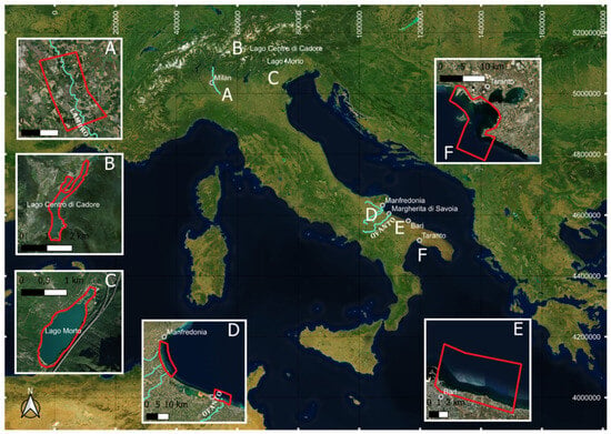
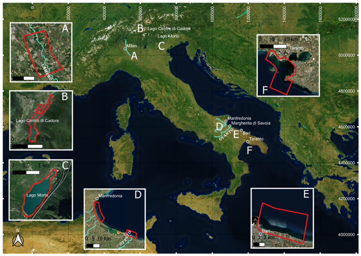
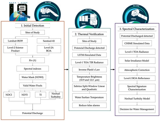
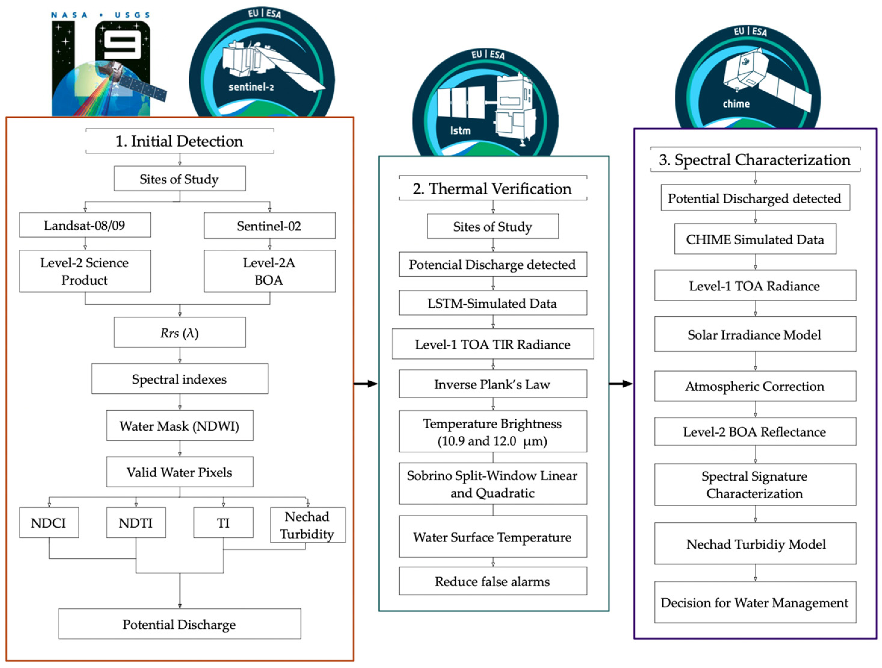
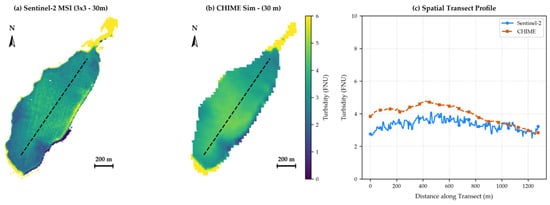
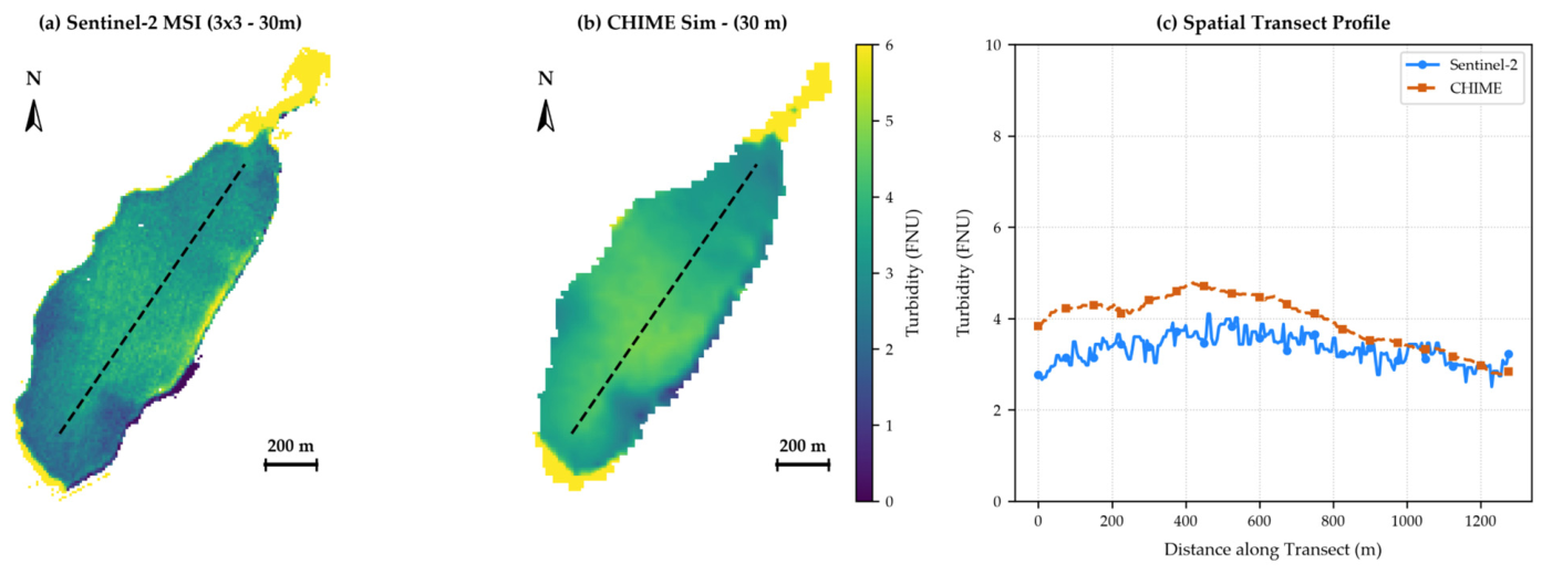
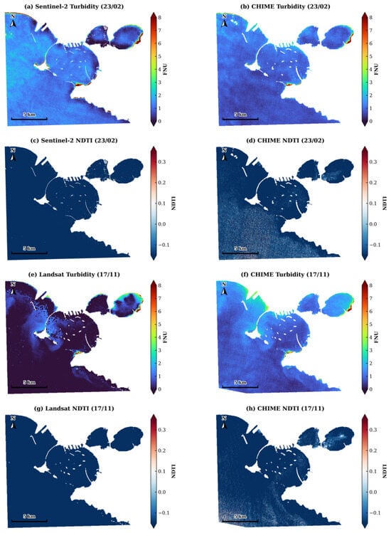
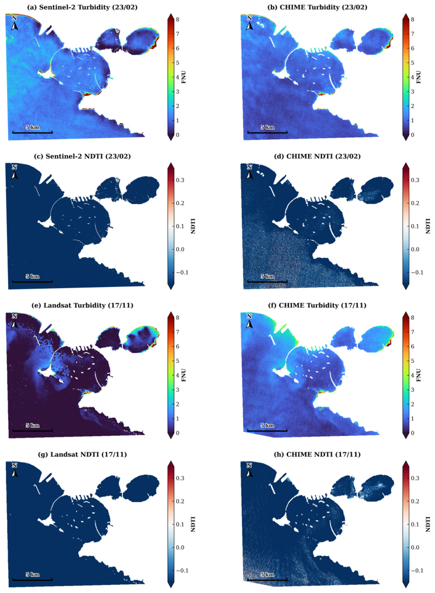
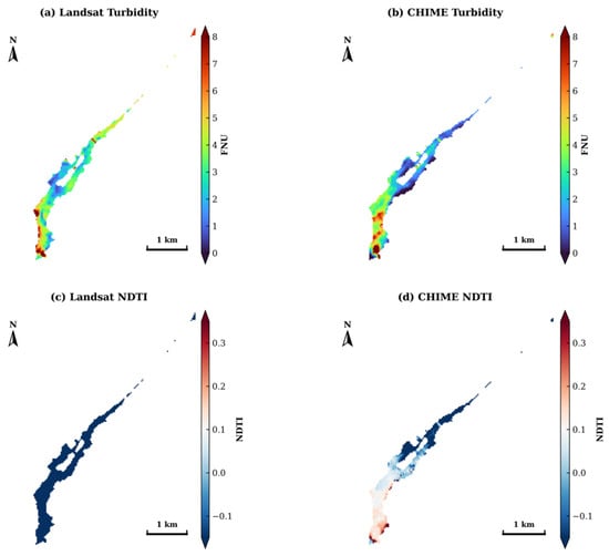
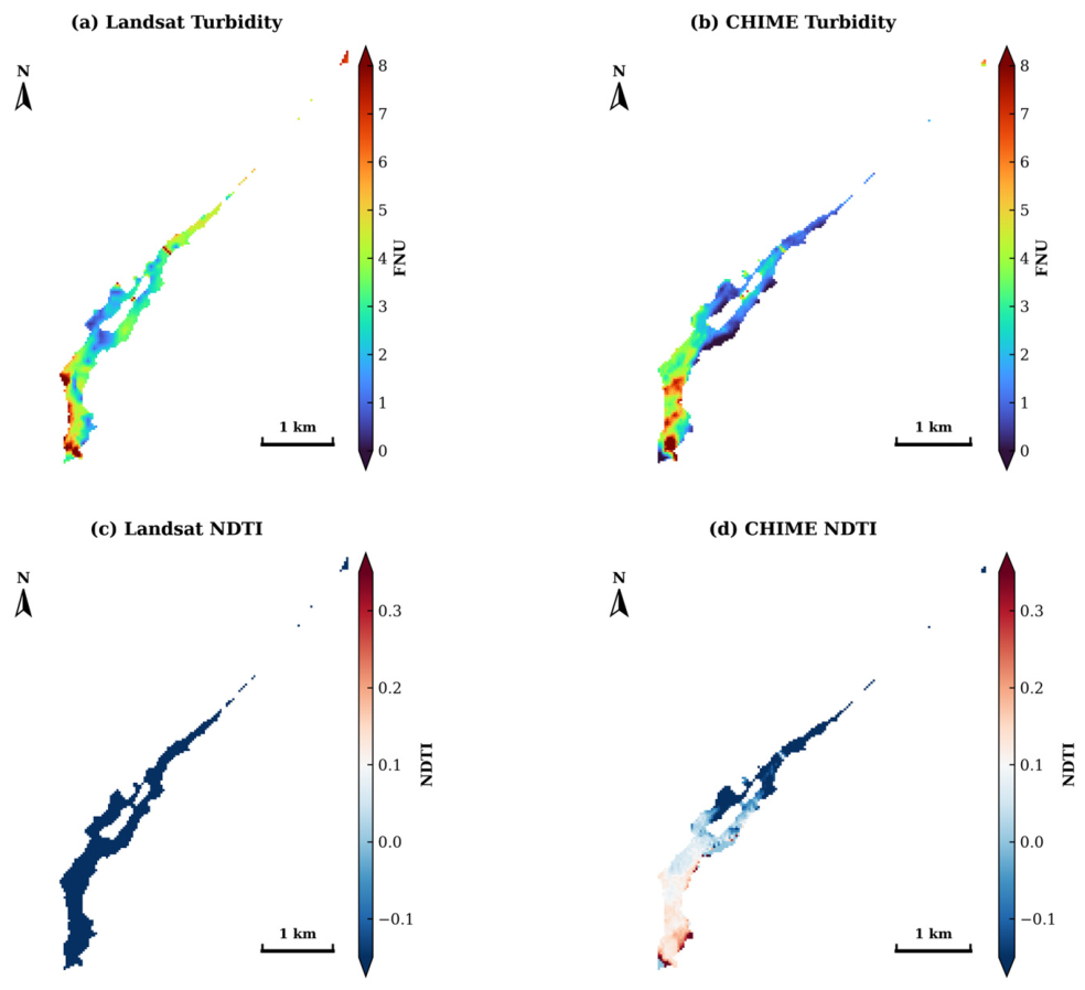
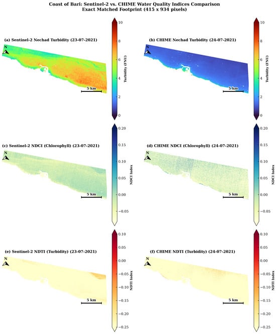
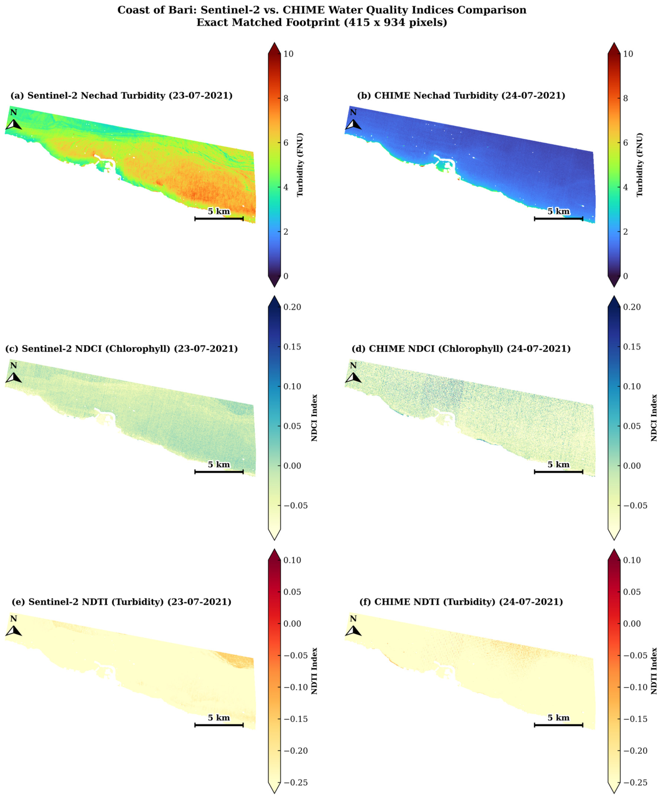
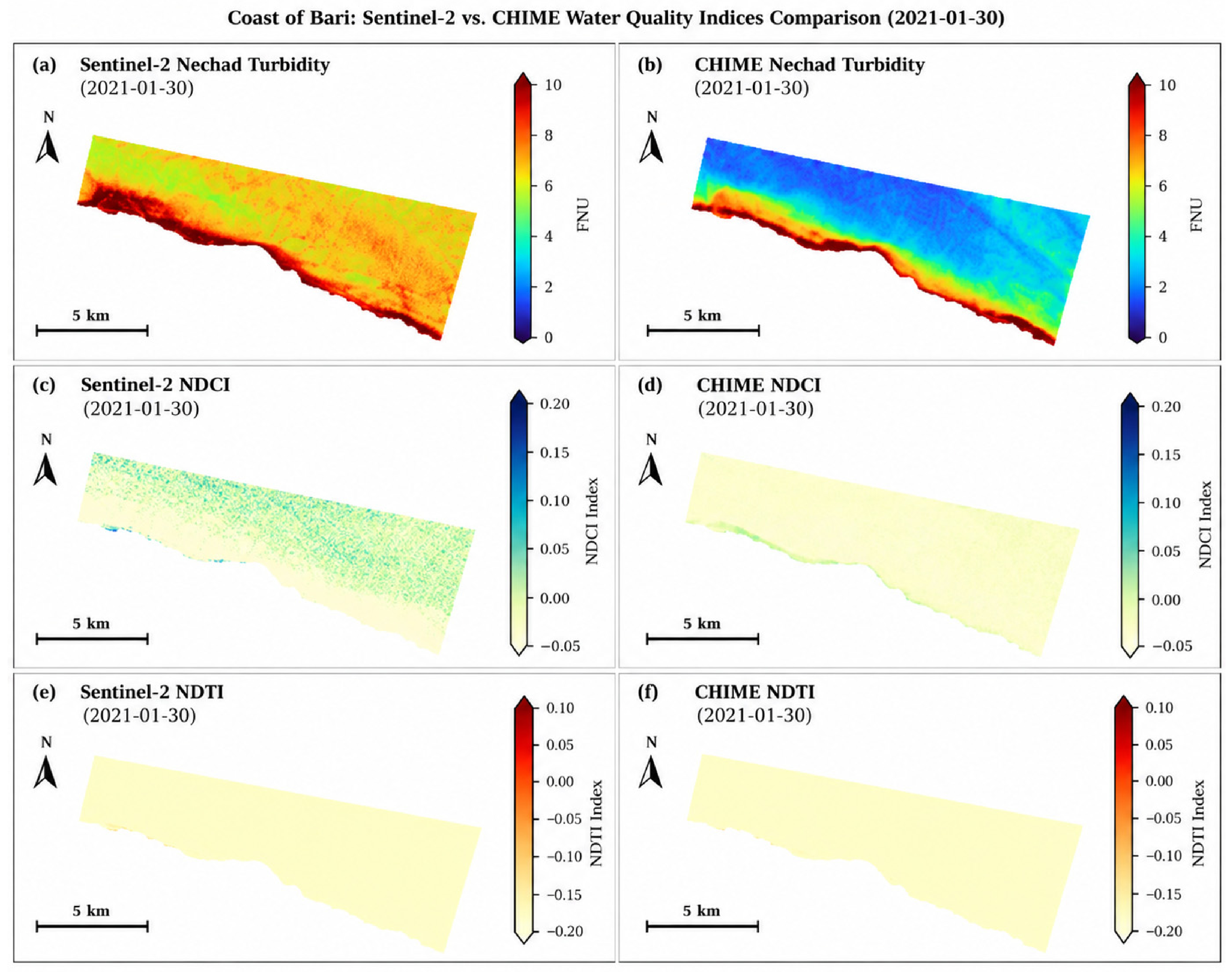
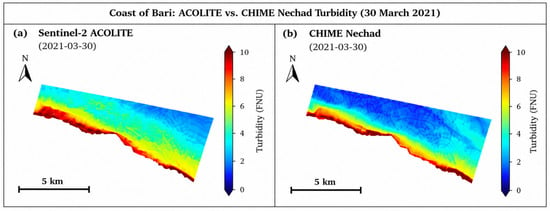
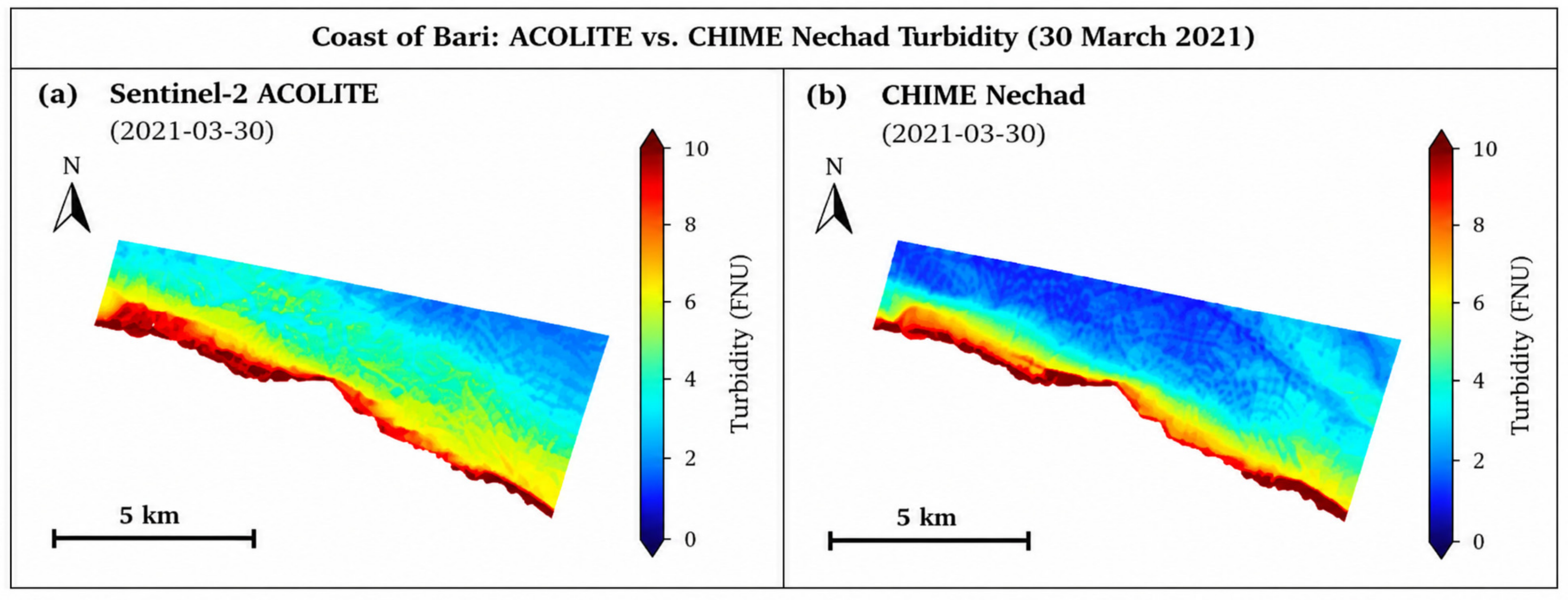
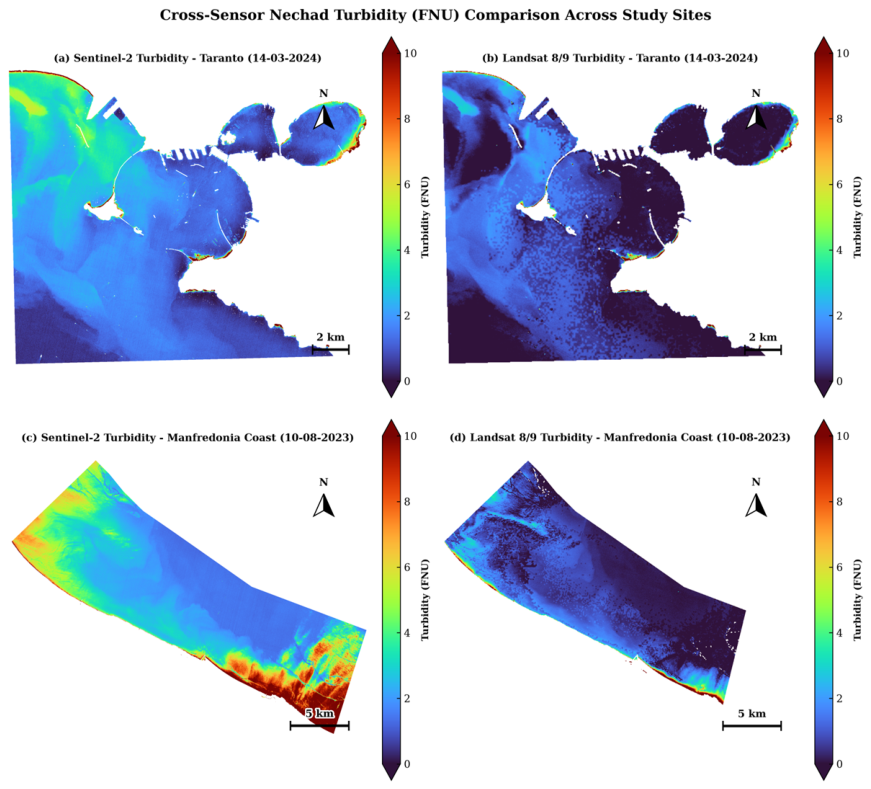
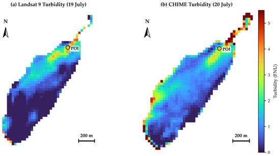
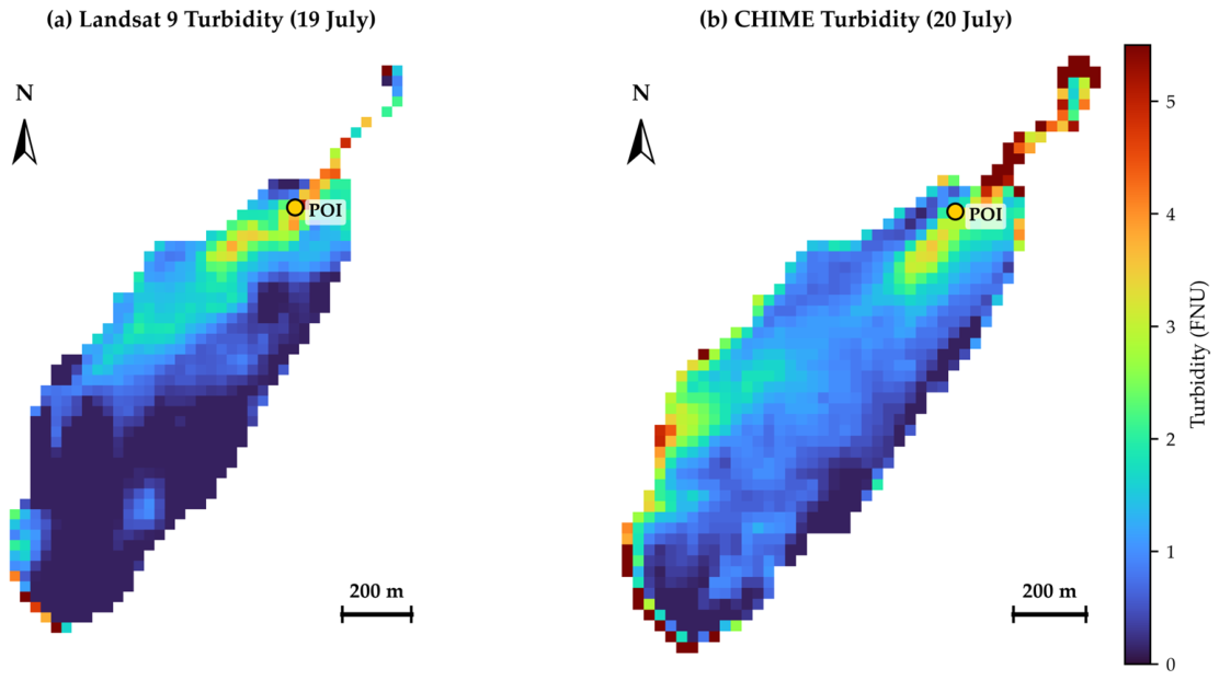
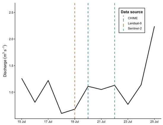
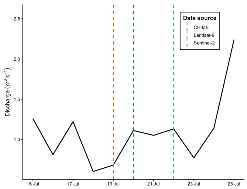
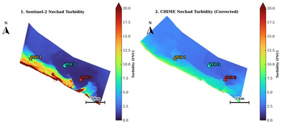
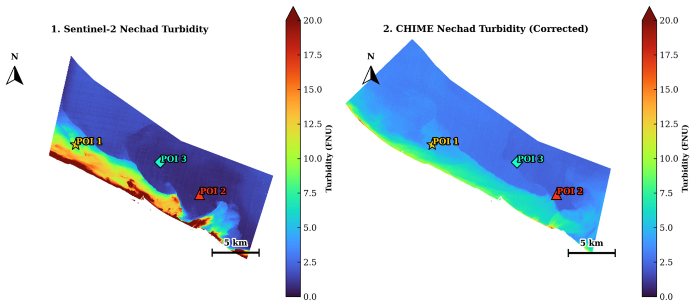
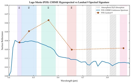
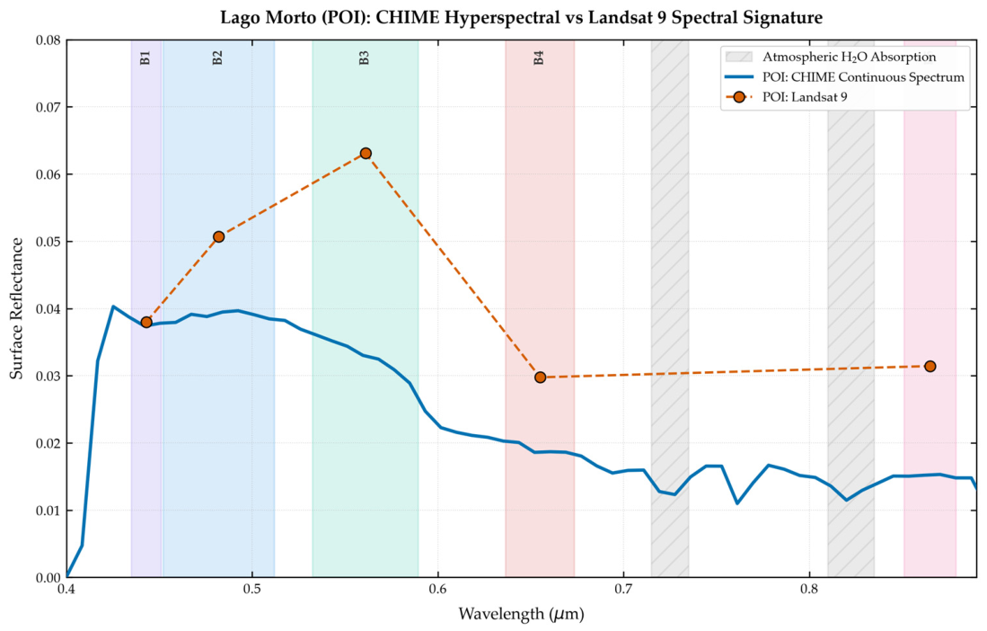
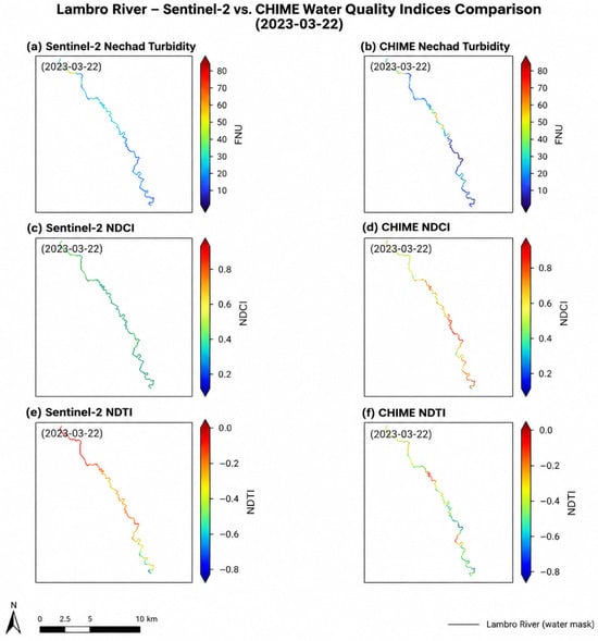
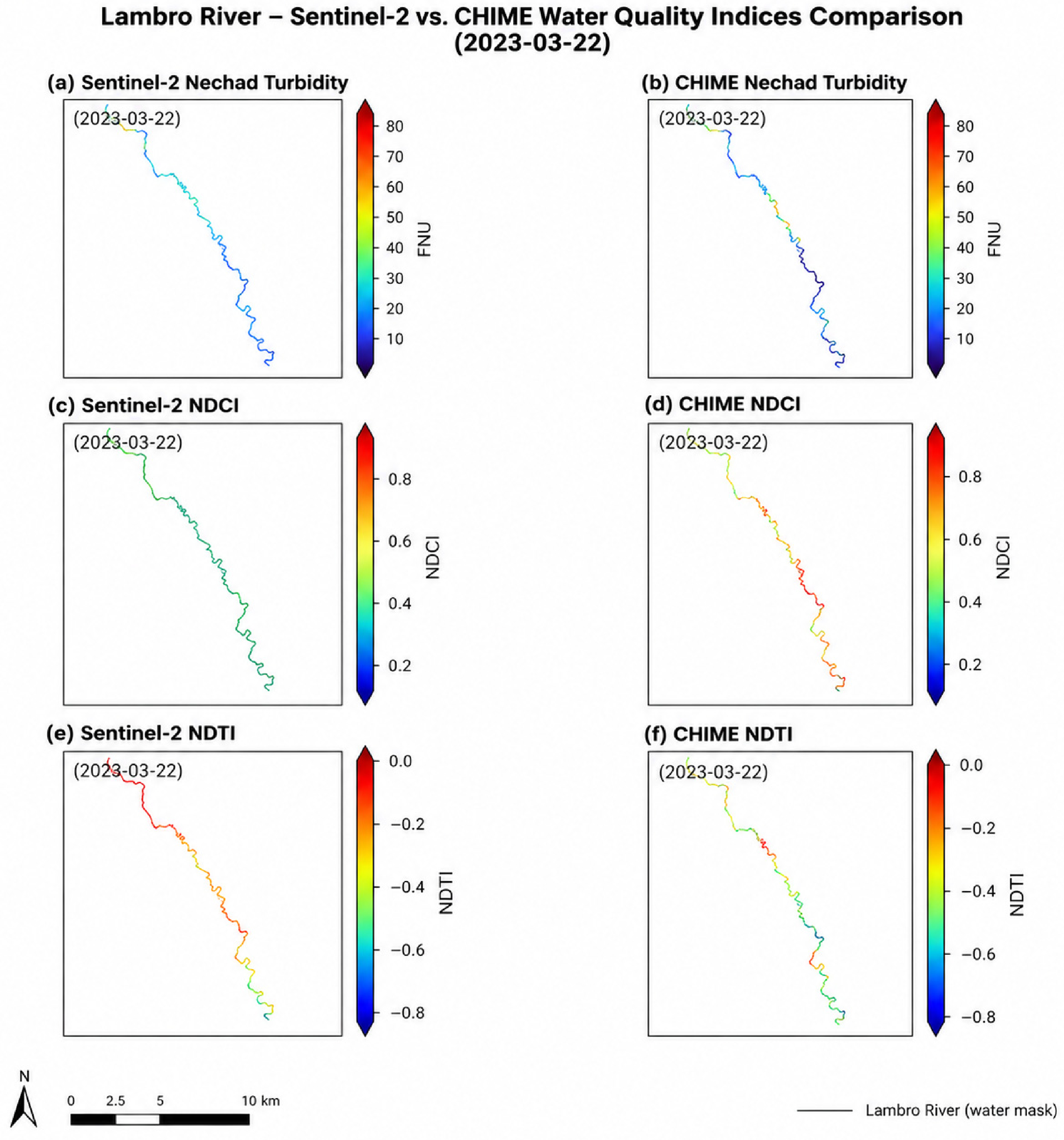
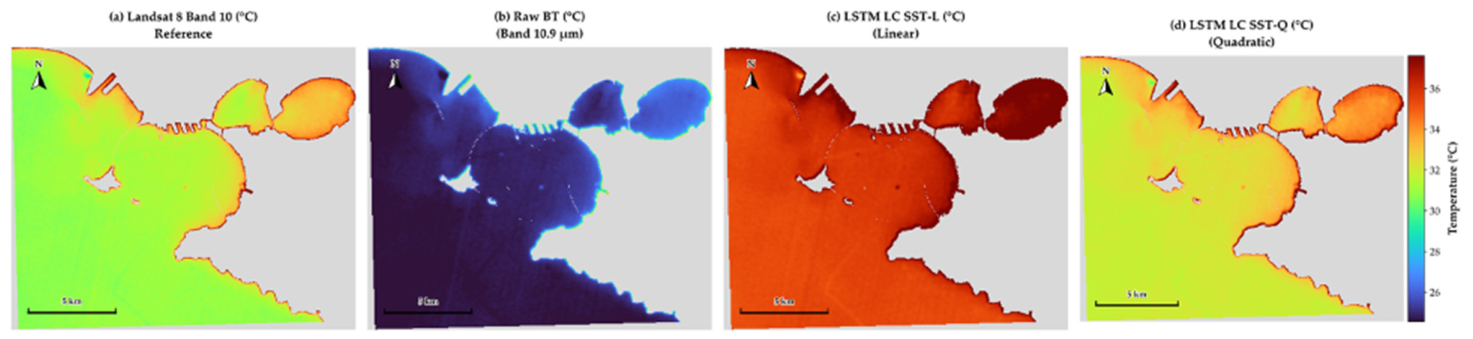
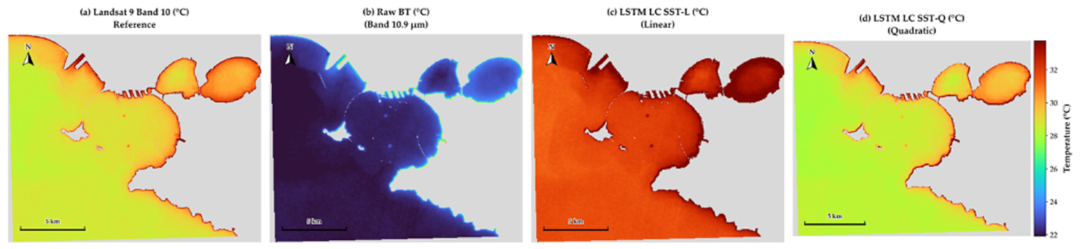
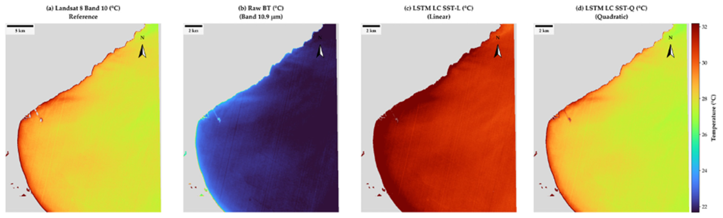
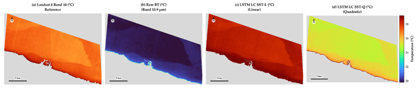
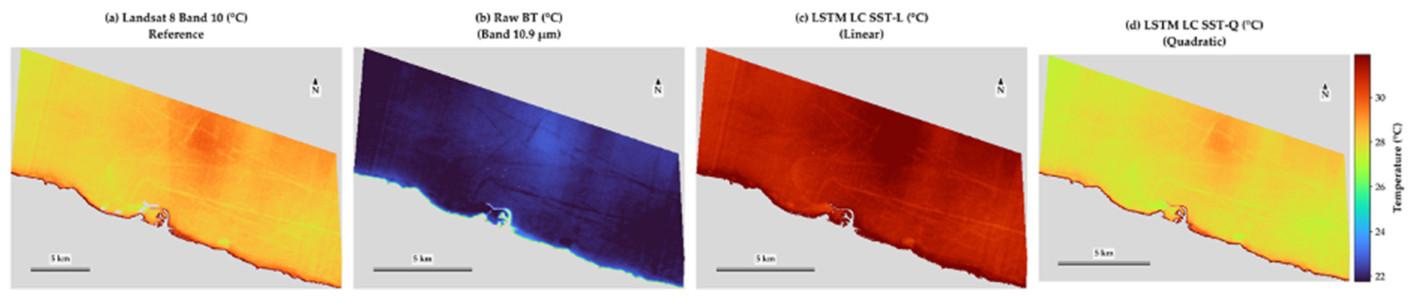
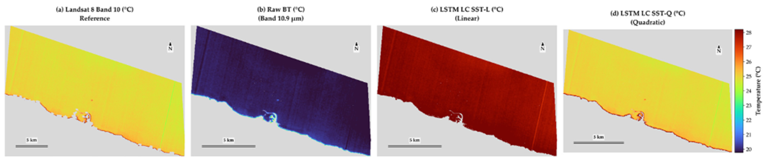

Disclaimer/Publisher’s Note: The statements, opinions and data contained in all publications are solely those of the individual author(s) and contributor(s) and not of MDPI and/or the editor(s). MDPI and/or the editor(s) disclaim responsibility for any injury to people or property resulting from any ideas, methods, instructions or products referred to in the content. |
© 2026 by the authors. Licensee MDPI, Basel, Switzerland. This article is an open access article distributed under the terms and conditions of the Creative Commons Attribution (CC BY) license.