


Highlights
What are the main findings?
- Spatial-block resampling identified the five-component diagonal GMM as the most reproducible shortlisted model of regional NDVI–NDMI trend patterns (median ARI = 0.912).
- The five archetypes revealed geographically distinct greenness–moisture patterns across Aseer, associated with contrasting terrain and land-cover conditions
What are the implications of the main findings?
- The identified regional patterns provide a basis for spatially targeted environmental monitoring and further ecological investigation
- Spatial reproducibility complements conventional fit diagnostics when selecting unsupervised remote-sensing classifications; superiority over annual or single-index clustering was not tested.
Abstract
This study examined whether joint vegetation-greenness and moisture-sensitive spectral trends across four standardized calendar windows form spatially reproducible archetypes in Aseer, Saudi Arabia, during 2015–2025, and how those archetypes relate to terrain and land cover. The normalized difference vegetation index (NDVI) and normalized difference moisture index (NDMI) were characterized via Kendall’s tau and Sen’s slope across four standardized three-month calendar windows. Gaussian mixture models (GMMs) with alternative component numbers and covariance structures were evaluated via spatial-block resampling, emphasizing geographic reproducibility rather than likelihood-based fit alone. Although higher-component models achieved more favorable likelihood criteria, the five-component diagonal GMM was substantially more reproducible, achieving a median adjusted Rand index of 0.912, normalized mutual information of 0.890, and centroid cosine similarity of 0.994. The resulting archetypes captured concordant positive, vegetation–moisture discordant, calendar-window-dependent, and weak or mixed trajectories. Terrain and land cover showed moderate environmental separability (balanced accuracy = 0.405), with elevation, local relief, and slope contributing most strongly. These findings reveal contrasting vegetation–moisture trend patterns across Aseer, with directional discordance concentrated in northern and northeastern interiors and positive or calendar-window-dependent trajectories prominent in western and southwestern mountain sectors. Spatial reproducibility provides a complementary criterion for selecting unsupervised classifications that support geographically meaningful environmental analysis.
1. Introduction
Semiarid mountain landscapes combine water limitation with abrupt gradients in elevation, slope, exposure, soil development, and moisture availability. These gradients generate pronounced environmental contrasts over short distances and can produce highly heterogeneous vegetation responses. In dryland mountain systems, drought sensitivity and greenness dynamics may vary with elevation and terrain position rather than following a uniform regional pattern [1,2,3]. Satellite remote sensing is therefore particularly valuable where field observations are sparse and where ecological responses are spatially discontinuous. Interpretation remains challenging because sparse vegetation, bright soil backgrounds, mixed land cover, and rugged terrain can affect spectral signals and limit assessments based on greenness alone [4,5,6,7].
The Aseer region of southwestern Saudi Arabia exemplifies this complexity. The region spans from coastal lowlands through steep escarpments to high-elevation mountain environments approaching 3000 m. Ecological studies in Aseer and adjacent southwestern mountain systems have shown that vegetation composition, density, regeneration, and degradation vary with elevation, slope orientation, local moisture availability, and human disturbance [8,9,10]. Remote-sensing studies have also documented substantial vegetation change over recent decades, but the direction and magnitude of change have not been spatially uniform [11]. Within the same broader mountain landscape, localized greening, vegetation decline, and woodland dieback may occur, underscoring the need for approaches that preserve spatial and temporal heterogeneity.
The normalized difference vegetation index (NDVI) is widely used to monitor vegetation greenness, but it does not directly measure ecosystem recovery, vegetation water content, or ecological conditions. Its performance may also be affected by soil-background reflectance in sparsely vegetated environments and by saturation in relatively dense vegetation [4,6]. Moisture-sensitive indices can provide complementary information. The normalized difference moisture index (NDMI), calculated from near-infrared and shortwave-infrared reflectance, is sensitive to moisture-related spectral variation and can help distinguish changes in greenness from changes in vegetation or surface moisture conditions. Joint NDVI–NDMI analysis can distinguish concordant greenness and moisture-sensitive tendencies from directional discordance. This is relevant where sparse cover, exposed soil and contrasting terrain conditions may influence the two spectral responses differently [12,13,14,15].
Temporal aggregation poses an additional challenge. Many vegetation monitoring studies rely on annual summaries or a single predefined seasonal period, commonly applying Mann–Kendall and Sen-slope estimators to detect monotonic trends [16,17,18]. However, vegetation responses in drylands depend on rainfall timing, temperature, short dry periods, and local terrain. Annual aggregation can reduce the visibility of contrasting calendar-window tendencies, although whether this four-window representation improves clustering or interpretation relative to an annual model was not tested here [19,20]. Four fixed three-month calendar windows—December–February (DJF), March–May (MAM), June–August (JJA) and September–November (SON)—were used as reproducible temporal strata. They were not selected from local phenology and should not be assumed to represent spatially uniform ecological seasons in Aseer. Two indices × two trend statistics × four windows yielded 16 model features; five archetypes were subsequently estimated by the GMM.
Large-area pixelwise trend analysis also requires careful handling of statistical support because repeated testing across numerous pixels and index–window combinations can inflate the apparent extent of significant change. False-discovery-rate correction can reduce this problem, while continuous trend direction and magnitude can be retained independently for trajectory characterization. This distinction allows statistical support to be evaluated without thresholding or removing weak but spatially coherent trajectory information.
Classifying multiwindow NDVI–NDMI trajectories poses a more fundamental methodological challenge because the number and structure of the underlying trajectory groups are unknown a priori. Gaussian mixture models provide a probabilistic framework for identifying overlapping multivariate patterns and estimating assignment uncertainty when independent class labels are unavailable [21,22,23]. However, conventional information criteria and internal separation metrics may favor increasingly complex solutions in very large spatial datasets without demonstrating that the inferred structure is geographically reproducible. The primary scientific contribution of this study is to characterize geographically differentiated vegetation–moisture trend patterns across Aseer during 2015–2025, using spatial reproducibility to evaluate the reliability of their unsupervised classification under changing geographic samples. Spatial-block resampling evaluated the geographic reproducibility of GMM classifications, while cross-method and rule-based comparisons assessed methodological sensitivity rather than ecological accuracy. The joint NDVI–NDMI features captured concordant and discordant spectral trends across four calendar windows, although superiority over annual or single-index approaches was not tested.
Environmental interpretation was conducted independently of archetype formation to avoid circularity. The resulting archetypes were characterized using terrain and land-cover variables, while spatially blocked modeling assessed their environmental separability without establishing causal relationships.
The study addresses three regional research questions: How are vegetation-greenness and moisture-sensitive trends spatially distributed across Aseer? Which distinct, spatially reproducible trend archetypes can be identified, and where do they occur? How do their geographical distributions relate to terrain and land-cover characteristics? Specifically, the study aimed to: (i) map the spatial distribution of NDVI and NDMI trend directions and magnitudes across four calendar windows; (ii) identify spatially reproducible multivariate trend archetypes and map their geographical distributions; and (iii) examine their associations with terrain and land cover and assess their environmental separability through spatially blocked validation.
2. Materials and Methods
2.1. Study Area
The Aseer region is a topographically and climatically heterogeneous mountain region in southwestern Saudi Arabia (Figure 1). The region extends from approximately 17.20°N to 20.50°N latitude and 41.30°E to 44.30°E longitude [24]. Its proximity to the Red Sea and transition from coastal lowlands to elevated escarpments and inland plateaus generate strong maritime–continental climatic gradients across short spatial distances. The elevation ranges from sea level to more than 3000 m, where orographic uplift produces pronounced windward–leeward contrasts, with wetter western slopes and warmer, drier eastern rain-shadow environments.
Figure 1.
Study area and topographic context of the Aseer region: (a) global location of Saudi Arabia; (b) administrative location of the Aseer region within Saudi Arabia; and (c) elevation across the study region.
Vegetation patterns reflect these climatic and topographic gradients. High-altitude environments support montane vegetation, juniper woodlands, and shrublands, whereas lower elevations are dominated by sparse xerophytic vegetation and drought-adapted grass communities [25,26].
2.2. Conceptual Framework
Figure 2 summarizes the analytical framework used to identify and interpret vegetation–moisture trajectory archetypes across the Aseer region. Landsat 8 OLI Collection 2 Tier 1 Level-2 surface-reflectance observations acquired from December 2014 to November 2025 were used to construct 11 annual analysis windows for 2015–2025. Clouds, cloud shadows, cirrus, snow, and radiometrically saturated observations were excluded via the QA_PIXEL and QA_RADSAT bands. Separate median composites were generated for DJF, MAM, JJA and SON from nominal 30 m Landsat source observations. The archived multivariate classification was stored on a 1450 × 1594-cell EPSG:4326 grid, with approximately 227 m east–west and 239 m north–south cell spacing near the study-area midpoint. For each analysis year y, DJF comprises December of year y−1 and January–February of year y. Therefore, DJF 2015 comprises December 2014 and January–February 2015; the 11 analysis years are 2015–2025. For each pixel and calendar window, Kendall’s tau describes the direction and consistency of monotonic change, whereas Sen’s slope quantifies its magnitude. Continuous NDVI and NDMI trend variables were assembled into a 16-dimensional feature matrix and classified via Gaussian mixture models. The candidate models were evaluated via information criteria, internal separation diagnostics, and spatial-block bootstrap stability. The maximum posterior probability, normalized entropy, and posterior margin characterize assignment confidence and ambiguity, whereas MiniBatch K-means and directional rule classifications provide methodological sensitivity comparisons. Copernicus DEM-derived terrain variables and ESA WorldCover 2021 were introduced only after clustering to characterize environmental associations and spatially blocked environmental separability without influencing archetype formation. The analytical sequence was designed to address the regional research questions. Mapping and area summaries established the geographic distribution of the retained archetypes, while independent terrain and land-cover comparisons and spatially blocked environmental modeling assessed their environmental associations. GMM selection and spatial-block resampling therefore served to establish a reproducible regional classification, while the resulting maps and environmental comparisons addressed the study’s geographical research objectives.
Figure 2.
Conceptual workflow for identifying and interpreting vegetation–moisture trajectory archetypes in the Aseer region.
2.3. Data Sources and Preprocessing
A multisource geospatial database supported trajectory mapping and environmental interpretation across Aseer. Landsat 8 surface-reflectance data (2014–2025) supplied NDVI and NDMI trend raster data. The Copernicus DEM provided terrain variables, ESA WorldCover characterized land cover and HDX administrative boundaries defined and clipped the study area for subsequent spatial analysis (Table 1).
Table 1.
Summary of the raster and vector geospatial datasets used in this study.
Landsat 8 Operational Land Imager (OLI) Collection 2 Tier 1 Level-2 surface-reflectance observations acquired from December 2014 to November 2025 were used to analyze annual multiwindow NDVI and NDMI dynamics across the Aseer region of southwestern Saudi Arabia [31,32,33,34]. The study area was covered primarily by the Worldwide Reference System-2 Path/Rows 165/44, 165/45, 166/44, and 166/45, which together provided complete regional coverage. A total of 2238 scenes intersected the study area. After a scene-level cloud cover threshold of less than 10% was applied, 1699 scenes were retained: 400 for December–February (DJF), 434 for March–May (MAM), 399 for June–August (JJA), and 466 for September–November (SON). Landsat Collection 2 reflectance scale factors and offsets were applied before index calculation. Clouds, cloud shadows, cirrus, snow, and radiometrically saturated observations were excluded via quality-assurance bands [32,34]. NDVI and NDMI were calculated for each quality-masked Landsat image to characterize vegetation greenness and moisture-related spectral variability:
where RED, NIR, and SWIR1 represent surface reflectances in the red, near-infrared, and first shortwave-infrared bands, respectively. For Landsat 8, the NIR band is Band 5, the RED band is Band 4, and the SWIR1 band is Band 6.
Pixelwise median index composites were then generated for each calendar window and analysis year during 2015–2025 to reduce residual noise while retaining within-year contrasts. DJF was assigned to the January–February year; thus, DJF 2015 covered December 2014–February 2015. No additional minimum-observation threshold was imposed; trend estimation used available annual composites at each analytical cell and window. Temporal coverage may vary among cells and calendar windows because no additional minimum-observation threshold was imposed.
2.4. Pixelwise Trend Metrics and Input Quality Control
For each index–calendar-window combination, monotonic change across analysis years 2015–2025 was characterized using Kendall’s rank correlation coefficient, whereas the magnitude of change was estimated using Sen’s slope [35,36].
Because tied observations may occur in remotely sensed time series, Kendall’s tau was used:
where and are the numbers of concordant and discordant observation pairs, respectively, and where and represent tied pairs in the two ranked variables. In this study, the first variable was the observation year, and the second variable was the corresponding NDVI or NDMI value.
The trend magnitude was estimated via Sen’s slope:
where and are index values observed at times and , respectively. Because the observations were summarized annually within each calendar window, represents the median change in index units per year. Sen’s slope is resistant to isolated extreme observations and does not require normally distributed residuals [35].
The combined use of Kendall’s and Sen’s slopes preserved two complementary properties of the time series: the consistency and direction of monotonic change and its estimated magnitude. These statistics were interpreted as spectral-index tendencies rather than direct measurements of ecological conditions.
2.5. Multiwindow Feature Engineering and Robust Scaling
A 16-variable feature vector was constructed for every complete analytical cell. Four variables were retained for each of the DJF, MAM, JJA, and SON calendar windows: the NDVI Kendall’s tau, robust-standardized NDVI Sen slope, NDMI Kendall’s tau, and robust-standardized NDMI Sen slope. This structure preserved the index-specific trend direction through Kendall’s τ and the relative change magnitude through the standardized Sen-slope features while avoiding the combination of the NDVI and NDMI into a single composite score [37]. Concordant, discordant, and calendar-window-dependent vegetation–moisture trajectories could therefore remain distinguishable in the multivariate feature space.
Because the dispersion of Sen slopes differed among indices and calendar windows, each of the eight slope layers was standardized over the analytical footprint using the median and median absolute deviation. The median absolute deviation was multiplied by 1.4826 to obtain a normal-consistent robust scale [38]. Extreme standardized values were clipped to ±8 to limit the influence of isolated distributional tails:
Because this transformation centered each slope distribution on its landscape-wide median, the sign of a standardized Sen-slope value was not necessarily the same as the sign of the original slope relative to zero. Standardized Sen-slope features were therefore interpreted as measures of relative change magnitude within each index–window distribution and were not used to determine the raw trend direction; directional interpretation was based on Kendall’s τ.
A second robust transformation was fitted only to the 80,000-pixel model development sample. Each of the 16 variables was centered on the training sample median and divided by its training sample interquartile range:
The fitted transformation was subsequently applied unchanged to the evaluation sample and the complete raster. This two-stage procedure first places the slope variables on comparable robust units and then prevents variables with greater dispersion from dominating the multivariate model.
The feature diagnostics included pairwise Pearson correlations, the multivariate condition number, and checks for near-zero interquartile ranges. One pair exceeded the predefined correlation threshold of : the robust NDVI slopes for DJF and SON (). The overall condition number was 12.27, and no feature had a near-zero interquartile range. Because redundancy was limited and every variable represented a prespecified index–window combination, all 16 features were retained.
2.6. Spatial Blocks and Held-Out Modeling Samples
The 1450 × 1594 analytical grid was divided into a separate 20 × 20 geographic-block layout (400 possible blocks), of which 292 contained complete analytical cells. Geographic blocks controlled spatially balanced sampling and resampling; the GMM fitted individual complete analytical cells, not block-average feature vectors. The development and evaluation samples contained 80,000 and 15,000 distinct cells, respectively, with no repeated cell between samples. They were not claimed to come from mutually disjoint geographic blocks. A 10,000-cell evaluation subset was used for computationally intensive internal clustering metrics. The relationship between raster cells and geographic blocks is illustrated in Supplementary Figure S3.
Block cross-validation is generally more appropriate than random cross-validation when spatial dependence is present because random splits can underestimate predictive error and encourage overfitting to noncausal spatial structures [39]. Spatial accuracy assessment in remote sensing likewise needs to account for spatial autocorrelation through spatial cross-validation or bootstrap procedures rather than nonspatial equivalents [40].
The held-out 15,000-pixel sample was used for partition-level comparisons between the GMM and MiniBatch K-means solutions, including the adjusted Rand index, normalized mutual information, and evaluation-sample agreement. Full-resolution outputs were used only to summarize the mapped agreement and component-specific correspondence.
Spatial-block identifiers were retained throughout the candidate-model assessment, bootstrap stability analysis, and environmental cross-validation. Pixels remained the observational units used to fit the models, but robustness and transferability were evaluated by resampling or withholding geographic blocks rather than relying only on random pixel divisions.
2.7. Gaussian Mixture Candidate Models and Diagnostic Screening
Probabilistic trajectory archetypes were estimated via finite Gaussian mixture models [41,42,43]. For a 16-dimensional feature vector , the observed distribution was represented as a weighted combination of multivariate Gaussian components:
Here x is the transformed 16-dimensional feature vector of an analytical cell, p(x) is its Gaussian mixture probability density, K is the number of components, k is the component index, πk is the component weight (πk ≥ 0 and Σkπk = 1), μk is the component mean vector, Σk is its covariance matrix, and N(x|μk, Σk) denotes the multivariate Gaussian density. In a diagonal-covariance GMM, each component has its own feature-wise variances and zero off-diagonal covariances; tied covariance uses a single shared covariance matrix.
Model development followed a two-stage candidate search. An initial assessment evaluated diagonal covariance models with 3–9. The search was subsequently extended to 3–15 under diagonal and tied covariance structures, yielding 26 candidate configurations. Diagonal covariance permitted component-specific variance for every feature while avoiding estimation of a full covariance matrix. Tied covariance provides a parsimonious alternative in which all the components share one covariance matrix [41].
The candidate models were fitted using k-means initialization, three independent initializations, covariance regularization of 10−5, random seed 42, and a maximum of 400 expectation–maximization iterations. The models were required to converge, retain all requested components, and maintain a minimum component proportion of 1% in the evaluation sample [44].
Diagnostic screening included the Bayesian information criterion, Akaike information criterion, integrated completed likelihood, held-out log-likelihood, silhouette coefficient, Calinski–Harabasz index, Davies–Bouldin index, mean maximum posterior probability, and normalized posterior entropy. Information criteria were not used as the sole basis for selecting the number of components because large spatial samples can favor increasingly fine partitions that are not geographically reproducible.
Five contrasting candidates were advanced for spatial stability assessment to represent the principal diagnostic alternatives identified during model screening. The diagonal , , and solutions represented the information criterion-leading high-complexity region, the tied covariance model represented the strongest low-dimensional separation solution on the basis of the silhouette coefficient, and the diagonal model represented the parsimonious solution retained from the initial assessment. All shortlisted models had already satisfied the basic admissibility requirements of convergence, retention of all requested components, and a minimum evaluation-sample component proportion of 1%.
2.8. Spatial-Block Bootstrap Selection of the Final GMM
Shortlisted models were evaluated via geographically structured bootstrap resampling. Twenty bootstrap replicates were generated for each candidate by sampling 80% of the 292 occupied model blocks. Each replicate was fitted using no more than 60,000 training pixels, one initialization, a maximum of 500 iterations, and covariance regularization of . All replicate models were evaluated against the same fixed 15,000-pixel evaluation sample.
Because component labels in mixture models are permutation invariant, replicate components were aligned with the corresponding reference components via minimum-cost Hungarian assignment [45]. Stability was evaluated via the adjusted Rand index (ARI), normalized mutual information (NMI), centroid distance and similarity, component-proportion error, component persistence, convergence, held-out likelihood, posterior confidence, and normalized entropy [46]. For final model comparison, six complementary stability diagnostics were ranked in their favorable directions: median ARI and median NMI from highest to lowest; median centroid Euclidean distance and median component-fraction mean absolute error from lowest to highest; median maximum posterior probability from highest to lowest; and median normalized entropy from lowest to highest. The six ranks were summed to obtain a consensus stability rank, with a smaller rank sum indicating greater overall reproducibility. Convergence and retention of the requested component structure were examined as additional admissibility diagnostics. The model with the smallest consensus rank sum was retained. The diagonal five-component model ranked first with a consensus rank sum of 6, compared with 17 for diagonal , 20 for diagonal , 20 for diagonal , and 27 for tied . The analysis retained a five-component diagonal GMM. The final estimator was refitted to the complete 80,000-pixel model sample via diagonal covariance, k-means initialization, three initializations, max_iter = 500, tolerance , covariance regularization , and random seed 42. The model converged after 17 expectation–maximization iterations. The component membership and posterior probabilities were then predicted for complete analytical cells [47,48,49,50].
The component numbers were assigned by the fitted model and subsequently given descriptive labels on the basis of their NDVI–NDMI direction and magnitude profiles. These labels summarize the observed spectral trajectories and do not represent field-validated ecological categories.
2.9. Probabilistic Assignment Uncertainty and Spatial Coherence
Three complementary posterior diagnostics were calculated for each analytical cell. The maximum posterior probability represents the probability assigned to the selected component. Normalized entropy quantifies the dispersion of membership probability across all five components:
For posterior membership pik, i indexes the analytical cell and k indexes the K components. Normalized entropy uses the full vector of pik values for each cell. The posterior margin is the difference between the largest and second-largest values among those K membership probabilities:
Large margins indicated clear separation from the next most likely component, whereas small margins indicated ambiguous assignment.
For diagnostic comparison, high-uncertainty cells were defined as those at or above the 90th percentile of normalized entropy. This threshold was used to determine whether uncertain assignments were disproportionately associated with disagreement between clustering approaches. It was not used to remove pixels or alter the final classification.
Spatial coherence was summarized via connected-component patch counts, patch size distributions, isolated-pixel frequencies, and orthogonal same-class adjacency. These measures describe spatial texture and fragmentation but are not treated as independent validations because external reference labels for the trajectory archetypes are unavailable [49].
2.10. Cross-Method and Rule-Based Sensitivity Analyses
Minibatch k-means with was fitted as a nonprobabilistic comparison method. Twenty independent runs used k-means++ initialization, batch_size = 4096, max_iter = 500, max_no_improvement = 50, and one initialization per seed. The solution with the lowest training inertia was retained. K-means labels were aligned with the GMM components via Hungarian assignment. Agreement was summarized via the adjusted Rand index, normalized mutual information, mapped percentage agreement, silhouette coefficient, Calinski–Harabasz index, and Davies–Bouldin index. These measures assess algorithmic consistency and are not interpreted as classification accuracy.
A directional-rule benchmark provided a second transparent sensitivity analysis. Every cell was assigned to one of five categories using the signs of the four NDVI and four NDMI Kendall tau values:
- Concordant positive, when at least three windows were positive for both indices;
- NDVI-positive/NDMI-mixed, when at least three NDVI windows were positive but the NDMI lacked three positive windows;
- NDVI-negative/NDMI-positive, when at least three NDVI windows were negative and at least three NDMI windows were positive;
- Concordant negative, when at least three windows were negative for both indices;
- Mixed directions for all remaining combinations.
The rule-based classes were compared with the GMM solution using the adjusted Rand index, normalized mutual information, Cramér’s , and Hungarian-matched agreement. Agreement between Kendall’s tau and Sen’s slope directions was summarized descriptively for each rule-based class [50,51].
2.11. Independent Terrain and Land Cover Predictors
For environmental characterization, the Copernicus DEM GLO-30 2024_1 dataset (COPERNICUS/DEM/GLO30_2024_1) and ESA WorldCover 2021 v200 (ESA/WorldCover/v200) in Google Earth Engine were used. Copernicus GLO-30 is a digital surface model and therefore represents the visible surface, including vegetation and built structures, rather than a bare-Earth terrain model. ESA WorldCover v200 provides 11 global land cover classes at 10 m spatial resolution from Sentinel-1 and Sentinel-2 observations [52].
The Copernicus DEM was processed in the WGS84/UTM zone 38 N at a 30 m working scale. Seven terrain variables were derived: elevation, slope, aspect, northness, eastness, topographic position index within a 300 m radius, and local elevation range within a 300 m radius. The circular aspect was transformed into continuous northness and eastness components:
The topographic position and local relief were calculated as follows:
Continuous terrain variables were aggregated by their mean to the exact trajectory-raster grid. The aspect was reconstructed through circular averaging of northness and eastness rather than arithmetic averaging of angular degrees. WorldCover classes were summarized at a 30 m working scale using the categorical mode, then aligned by nearest-neighbor resampling to the coarser trajectory-raster grid (approximately 227 × 239 m near the study-area midpoint).
Quality-control checks confirmed agreement in raster dimensions, coordinate reference system, affine transformation and grid alignment. The corrected terrain and WorldCover predictors covered all complete analytical cells.
2.12. Archetype-Level Environmental Characterization
Environmental summaries were calculated independently for each trajectory archetype. Pixel-level area-weighted statistics describe terrain conditions and land-cover composition, whereas spatial-block summaries reduce the influence of local pixel autocorrelation.
For each continuous terrain variable and archetype, medians were first calculated within the occupied spatial blocks. Component–variable combinations represented by fewer than 30 pixels within a block were excluded. The median of the block medians was reported together with the interquartile range and 95% percentile confidence intervals derived from 1000 block-bootstrap replicates.
The WorldCover composition was expressed as the area percentage of each land-cover class within each archetype. Spatial uncertainty was estimated by resampling occupied blocks 1000 times. The degree of land cover enrichment was calculated as the ratio between the proportion of the land cover class within the archetype and its proportion across the full analytical landscape:
indicates relative enrichment, indicates underrepresentation, and indicates representation proportional to the landscape-wide composition. For visualization and comparison, enrichment ratios were also transformed into , for which positive values indicated enrichment, negative values indicated underrepresentation, and zero values indicated proportional representation. These analyses were descriptive and associative. Differences among archetypes were not interpreted as evidence of causal environmental control, and WorldCover was not treated as reference data for the unsupervised classes.
2.13. Spatially Blocked Environmental Separability Model
A supervised environmental model was used only to quantify the extent to which terrain and land cover variables could discriminate among the five trajectory archetypes in geographically withheld areas. The predictor matrix contained six continuous terrain variables—elevation, slope, northness, eastness, , and local relief—and nine one-hot WorldCover indicators representing tree cover, shrubland, grassland, cropland, built-up land, bare or sparse vegetation, permanent water, herbaceous wetland, and mangroves. The aspect in degrees was excluded because its directional information was already represented by northness and eastness.
To balance geographic and class representations, up to 120 pixels were sampled from every spatial block × archetype combination. The final modeling dataset contained 111,092 pixels distributed across all 292 occupied blocks. The response variable was the GMM component number; model performance therefore represented the environmental separability of the derived archetypes rather than independent ecological accuracy.
A HistGradientBoostingClassifier was fitted via log loss, learning_rate = 0.07, l2_regularization = 1.0, max_leaf_nodes = 31, min_samples_leaf = 40, max_bins = 255, early stopping, validation_fraction = 0.10, n_iter_no_change = 20, tolerance , and random seed 42. Maximum iteration limits of 250, 500, and 750 were evaluated. All the folds fitted with 250 iterations reached the specified limit, whereas the 500- and 750-iteration configurations stopped naturally and produced effectively equivalent performance and predictor rankings. A maximum of 500 iterations was therefore retained.
Spatial transferability was evaluated via fivefold stratified group K-fold cross-validation. A spatial-block identifier was used as the grouping variable, ensuring no overlap between the training and test blocks while approximately preserving the component proportions. The performance was summarized in terms of overall accuracy, balanced accuracy, macro- and weighted F1 scores, Cohen’s kappa, multiclass log loss, confusion matrices, and component-specific precision, recall, and F1. Balanced accuracy and macro-F1 scores were emphasized because the archetype prevalence was unequal.
2.14. Grouped Permutation Importance and Robustness Analyses
Predictor importance was evaluated within each held-out spatial fold via grouped permutation, and the decrease in balanced accuracy was used as the scoring measure. The six continuous terrain variables were permuted independently. All nine WorldCover dummy variables were permuted so that land cover remained interpretable as one categorical predictor. Five permutation repetitions were performed for every predictor group and were performed with up to 20,000 test pixels.
Fold-specific importance values were summarized by their mean, standard deviation, minimum, maximum, and within-fold permutation variability. Because importance was calculated via geographically withheld observations, it represented spatially transferable predictive information rather than in-sample associations [53].
Two analyses tested whether the environmental conclusions depended on model duration or spatial partitioning. First, the same five folds were evaluated using maximum iteration limits of 250, 500, and 750. The performance, prediction agreement, and predictor—rank correlation were compared across these configurations. Second, the complete 111,092-pixel dataset and fixed model parameters were evaluated via , , , and spatial-block grids. These corresponded to approximate block dimensions of 21.92 × 25.36 km, 16.44 × 19.02 km, 13.15 × 15.22 km, and 10.96 × 12.68 km, respectively.
Robustness was evaluated from the ranges of balanced accuracy, macro-F1, and Cohen’s kappa; prediction agreement among block configurations; Spearman rank correlations of grouped importance; and consistency of the dominant predictor. The prespecified grid was retained as the primary validation design.
2.15. Software, Randomization, and Reproducibility
Raster processing, spatial analysis, and statistical modeling were conducted in Python 3.12.13 via NumPy 2.0.2, pandas 2.2.2, SciPy 1.16.3, scikit-learn 1.6.1, Matplotlib 3.10.0, rasterio 1.5.0, GeoPandas 1.1.4, pyproj 3.7.2, and joblib 1.5.3. Google Earth Engine processing was performed with earthengine-api 1.7.35 and geemap 0.38.3. Machine learning algorithms were implemented via scikit-learn [54].
3. Results
3.1. Analytical Coverage
Complete NDVI–NDMI trajectory profiles covered 99.98% of the analytical footprint (76,968.22 km2). Median Kendall’s τ was positive for both indices across all four calendar windows, with varying trend strengths. Spatial maps of Kendall’s τ and raw Sen’s slope for both indices and all four calendar windows are provided in Supplementary Figure S1, with consistent colour scales within each index–metric combination.
3.2. GMM Selection and Spatial Reproducibility
The candidate model diagnostics did not identify a single optimum across the tested Gaussian mixture models. The 15-component diagonal model produced the lowest Bayesian information criterion (BIC) and integrated completed likelihood (ICL), together with the highest independent-evaluation log-likelihood, whereas the three-component tied-covariance model produced the highest silhouette score. The diagnostic criteria therefore favored markedly different levels of model complexity (Figure 3). BIC and ICL were treated as measures of relative mixture—density fit rather than as definitive indicators of the most appropriate spatial classification. Given the very large analytical sample, small improvements in likelihood could strongly favor additional components and increasingly fine statistical partitions. These subdivisions were not considered sufficient unless they were also reproducible when geographically distinct portions of the study area were resampled. The final model selection was therefore based on spatial block stability, while conventional fit statistics were retained as diagnostic screening criteria.
Figure 3.
Extended assessment of candidate Gaussian mixture models across three to fifteen components under diagonal and tied covariance structures. Panels show (A) the Bayesian information criterion, (B) the integrated completed likelihood, (C) the silhouette coefficient calculated via the independent evaluation sample, and (D) the mean independent-evaluation log-likelihood per pixel. Lower BIC and ICL values and higher evaluation log-likelihood values increasingly favored higher-component diagonal models, whereas the silhouette coefficient favored a three-component tied-covariance model. Because these criteria support different levels of complexity, the final model selection was based on spatial block reproducibility rather than on likelihood-based diagnostics alone.
Five contrasting candidates were advanced to spatial-block stability assessment: diagonal covariance models with 5, 13, 14, and 15 components and a three-component tied covariance model (Table 2). Although the five-component diagonal model ranked 24th by the BIC among the 26 candidate configurations, it ranked first in the joint spatial-stability assessment, with a consensus rank sum of 6 compared with 17–27 for the other shortlisted models. All 20 resampling repetitions converged, and the five-component model achieved a median adjusted Rand index of 0.912 (interquartile range, 0.870–0.919; minimum, 0.779), median normalized mutual information of 0.890, median centroid cosine similarity of 0.994, and median component-fraction MAE of 0.0086. The complete five-component structure was retained in every repetition. The higher-component diagonal models achieved more favorable likelihood-based diagnostics but substantially lower spatial reproducibility, with median adjusted Rand indices of 0.443–0.538. The five-component diagonal GMM was therefore retained as the highest-ranked geographically reproducible representation of the dominant multiwindow NDVI–NDMI trajectory structure.
Table 2.
Spatial-block bootstrap comparison of shortlisted Gaussian mixture models.
3.3. Multi-Window NDVI-NDMI Trajectory Archetypes
The retained model resolved five joint spectral-trend archetypes (Table 3): C1, greenness–moisture directional discordance; C2, moderate concordant positive tendencies; C3, positive greenness with calendar-window-dependent moisture-sensitive tendencies; C4, strong concordant positive tendencies; and C5, weak or mixed tendencies. C1 was the largest class (21,976.93 km2, 28.55% of the analyzed area). These descriptors refer to satellite-observed tendencies and do not establish ecological recovery, degradation or stability.
Table 3.
Area, descriptive spectral-trend labels, calendar-window NDVI–moisture-index signatures and assignment diagnostics for the five-component GMM.
C1 presented a weakly negative median NDVI Kendall’s τ across all four calendar windows, ranging from −0.128 to −0.051. In contrast, the median NDMI Kendall’s τ remained consistently positive, ranging from 0.273 to 0.455. The standardized Sen-slope features used in the GMM represented the relative change magnitude within each index–window distribution and were not interpreted as indicators of the raw trend direction. C1 was therefore described as greenness–moisture directional discordance, not straightforward vegetation decline or a field-confirmed ecological state.
Across the four calendar windows, the five components exhibited distinct combinations of greenness and moisture-sensitive spectral trends (Supplementary Figure S2). For C3, the saved moisture-index median Kendall τ was positive in DJF (0.127) and SON (0.236), whereas it was near neutral or negative in MAM (−0.018) and JJA (−0.091). Raw Sen slopes and Kendall τ are displayed separately because τ is dimensionless and slope is expressed in index units per year. These contrasts are descriptive; they do not demonstrate that the four-window representation outperforms an annual or single-index alternative.
The five spectral-trend components were differentiated by continuous multiwindow direction and relative magnitude; component-level calendar-window profiles are shown in Supplementary Figure S2.
3.4. Spatial Distribution, Assignment Confidence, and Cross-Method Consistency
The five archetypes exhibited geographically differentiated distributions across Aseer (Figure 4b). C1, representing greenness–moisture directional discordance, was concentrated in the northern and northeastern interiors. C3, characterized by calendar-window-dependent moisture-sensitive trends, occurred mainly along western and southwestern mountain corridors, whereas C4, representing strong concordant positive greenness–moisture tendencies, was prominent in western and southwestern high-relief belts. C2 and C5 extended across substantial central and interior areas. These distributions reveal contrasting regional spectral trajectories rather than a geographically uniform greening or browning response.
Figure 4.
Comparison of the matched five-cluster MiniBatch K-means and five-component diagonal Gaussian mixture model (GMM) classifications in Aseer. (a) Matched K-means class map; (b) GMM class map; (c) agreement and disagreement between methods; (d) GMM maximum posterior probability; and (e) normalized GMM posterior entropy. Identical component colors are used after Hungarian matching. Agreement is a measure of methodological consistency, not independent ecological classification accuracy.
Across the full map, 79.16% of the valid adjacent pixel pairs shared the same component label. Isolated pixels represented 1.81% of the analytical area, whereas 4.73% of the pixels occurred in patches containing fewer than five cells. These results indicate substantial spatial coherence, although the metrics are descriptive and do not constitute independent validation.
The assignment confidence was high overall. The mean maximum posterior probability was 0.957, the median was 0.9999, and the mean posterior margin was 0.916. The mean normalized entropy was 0.0648, indicating generally low assignment ambiguity (Figure 4d,e). C3 had the highest mean entropy (0.088), followed by C2 (0.081), whereas C1 had the lowest mean entropy (0.045). Most cells were therefore assigned decisively, although localized areas of greater ambiguity occurred near boundaries between component distributions.
After component matching, the full-map agreement between GMM and MiniBatch K-means was 75.93% (Figure 4c). Agreement was highest for C1 (98.73%) and C5 (93.78%), intermediate for C2 (72.60%), and lower for C4 (47.43%) and C3 (32.48%). These differences indicate that C1 and C5 were reproduced consistently under both clustering algorithms, whereas C3 and C4 were more sensitive to the underlying clustering formulation.
Compared with 20.91% among cells below this threshold, 52.46% of the cells within the upper entropy decile, defined by normalized entropy ≥ 0.289, exhibited GMM–K-means disagreement. The corresponding disagreement risk ratio was 2.51. Normalized entropy distinguished agreement from disagreement, with a diagnostic area under the receiver operating characteristic curve of 0.710. This association indicates that posterior assignment ambiguity and cross-algorithm disagreement are spatially related. However, neither measure represents ecological error or classification accuracy in the absence of independent reference data.
The transparent directional rule benchmark showed substantially lower correspondence with the GMM, with an adjusted Rand index of 0.218, normalized mutual information of 0.336, and mapped agreement of 49.28% (Table 4, panel A). This lower correspondence was expected because the rule-based approach reduced continuous multiwindow trajectory information to discrete directional categories. The directional-rule comparison was therefore treated as a transparent sensitivity assessment rather than as validation of the GMM classification.
Table 4.
Cross-method sensitivity of the final five-component GMM classification.
Additional relationships among posterior ambiguity, GMM–K-means agreement, and spatial coherence are presented in Figure 5.
Figure 5.
Relationships among assignment ambiguity, cross-method agreement, and spatial coherence. Panels show (A) GMM–K-means agreement across normalized-entropy deciles, (B) agreement by the GMM component, (C) the proportion of pixels occurring in small patches, and (D) different-class adjacency and isolated-pixel percentages for the GMM and MiniBatch K-means solutions. These diagnostics describe assignment ambiguity, methodological consistency, and mapped spatial structure; they do not constitute independent ecological validation.
3.5. Terrain and Land-Cover Associations
Terrain and land cover clearly differed among the five trajectory archetypes (Figure 6 and Figure 7). Component 1 occurred predominantly on comparatively gentle terrain, with a median elevation of 1135 m, median slope of 0.98°, and median local relief of 10.0 m. Component 2 occupied the highest median elevation, at 1753 m, but was associated with only moderate slopes. Components 3 and 4 occurred on the steepest and most dissected terrains: their median slopes were 15.55° and 14.01°, respectively, whereas the median local relief reached 117.83 m and 106.03 m. Component 5 occupied intermediate elevation, slope, and relief conditions.
Figure 6.
Terrain, land cover context, and spatial distribution of the five multiwindow NDVI–NDMI trajectory archetypes in the Aseer region. Panels show (A) elevation, (B) slope, (C) local relief within a 300 m neighborhood, (D) topographic position index within a 300 m neighborhood, (E) ESA WorldCover 2021 classes, and (F) the final five-component diagonal Gaussian mixture model trajectory-archetype classification.
Figure 7.
Environmental associations of the five multiwindow NDVI–NDMI trajectory archetypes. Panel (A) shows robust standardized differences between each archetype median and the landscape median for elevation, slope, northness, eastness, topographic position index, and local relief. Panel (B) shows the enrichment of selected ESA WorldCover classes within each archetype relative to their landscape-wide proportions. Positive values indicate above-landscape terrain medians or land cover enrichment, whereas negative values indicate below-landscape medians or underrepresentation. The values describe spatial associations rather than causation.
Bare or sparse vegetation accounted for 88.44% of the analytical area and was the dominant WorldCover class within every archetype. Its share exceeded 98.9% for Components 1, 2, and 5 but declined to 52.28% for Component 3 and 64.90% for Component 4. Component 3 contained 23.07% shrubland and 21.02% grassland, with grassland showing an enrichment ratio of 5.07 relative to its landscape-wide proportion. Component 4 contained 23.03% shrubland and 9.67% grassland. Although tree cover occupied only a small absolute area, it showed the strongest relative enrichment within Component 4, with an enrichment ratio of 4.60.
Together with the mapped distributions (Figure 6F), these contrasts distinguish the predominantly sparse, gently sloping northern and northeastern C1 interiors from the steeper western and southwestern mountain sectors occupied by C3 and C4, where shrubland and grassland are more prominent. The combined spatial distributions of the terrain, land cover, and trajectory archetypes are presented in Figure 6, whereas the robust-standardized terrain differences and land cover enrichment are summarized in Figure 7. These patterns represent spatial associations and should not be interpreted as evidence of causal environmental control or independent ecological validation. Component-level median elevation, slope and relief are also compared in Supplementary Figure S4.
3.6. Spatially Blocked Environmental Separability
The environmental model used 111,092 observations distributed across all 292 occupied spatial blocks. Fivefold stratified group cross-validation maintained complete separation between training and held-out blocks in every fold. The resulting performance therefore quantified the extent to which the terrain and land cover variables could distinguish the five GMM trajectory archetypes in geographically withheld areas rather than their ecological accuracy.
For the retained 500-iteration configuration, overall accuracy was 0.394, balanced accuracy was 0.405, macro-F1 was 0.382, Cohen’s κ was 0.243, and multiclass log loss was 1.355 (Table 5; Figure 8A). The fold-level balanced accuracy ranged from 0.394 to 0.420, with a standard deviation of 0.012. Although the balanced accuracy exceeded the five-class reference value of 0.20, the results indicated limited-to-moderate environmental separability rather than complete discrimination among the trajectory archetypes.
Table 5.
Spatially blocked environmental model performance and robustness.
Figure 8.
Spatially blocked environmental separability of the five multiwindow NDVI–NDMI trajectory archetypes. Panels show (A) balanced accuracy, macro F1, and Cohen’s for each spatial cross-validation fold; (B) the row-normalized confusion matrix, expressed as the percentage of each observed component assigned to the five predicted components; (C) spatially cross-validated recall by trajectory archetype; and (D) grouped permutation importance, expressed as the decrease in balanced accuracy following predictor—group permutation. The dashed reference value of 0.20 applies to balanced accuracy in panel (A) and component recall in panel (C); it is not a reference value for macro F1 or Cohen’s . Performance and predictor importance quantify environmental separability and associations rather than ecological validation or causal control.
The environmental separability differed markedly among the components (Figure 8B,C). Recall was highest for C1 (0.661), followed by C5 (0.458), C4 (0.398), Component 3 (0.348), and C2 (0.162). C2 was most frequently confused with C1 and C5, whereas C3 and C4 showed substantial mutual confusion. These patterns indicate considerable environmental overlap among some of the trajectory archetypes, particularly between classes occupying similar elevation, terrain, or land-cover settings.
Grouped permutation importance identified elevation as the most informative environmental predictor, producing a mean decrease in the balanced accuracy of 0.0969 after permutation. Local relief was the second most important predictor (0.0527), followed by slope (0.0514), the topographic position index at 300 m (0.0329), and the jointly permuted WorldCover predictor group (0.0303). Eastness (0.0105) and northness (0.0038) contributed comparatively little (Figure 8D).
The environmental variables therefore contained reproducible information about the spatial organization of the trajectory archetypes but did not fully reproduce the remote-sensing classification. Their importance should consequently be interpreted as evidence of environmental associations and spatial separability rather than causal control.
3.7. Convergence and Spatial-Scale Robustness
Sensitivity analyses yielded similar aggregate environmental-separability metrics across the tested boosting limits and spatial-block configurations. Detailed iteration histories, block-grid comparisons and predictor-importance diagnostics are provided in Supplementary Tables S1 and S2 and Supplementary Figures S6 and S7.
4. Discussion
4.1. Multiwindow Trend Characterization and Geographic Reproducibility
Kendall’s τ and Sen’s slope summarized monotonic direction and magnitude in each of four calendar windows, permitting direct comparison of within-year differences in the archived spectral-trend summaries. These periods were treated as standardized calendar windows rather than uniform ecological seasons across Aseer’s strong elevation and climatic gradients. Recent remote-sensing studies similarly demonstrated that vegetation responses can differ among spectral indicators and temporal periods, particularly under moisture-limitation conditions [55,56].
The principal regional finding is that vegetation-greenness and moisture-sensitive trends across Aseer are organized into geographically differentiated archetypes rather than a uniform regional response. Geographic reproducibility was important for distinguishing persistent regional structure from classification patterns sensitive to changes in geographic sampling. Although higher-component GMMs achieved stronger likelihood-based fit, the five-component diagonal model was the most reproducible shortlisted solution (median ARI = 0.912). This methodological result supports the reliability of the broad regional partition under the tested resampling design but does not establish ecological ground-truth accuracy or a uniquely correct ecological classification [57,58,59].
The importance of this reproducibility assessment lies in supporting the interpretation of Aseer’s regional vegetation–moisture patterns, rather than identifying a uniquely correct ecological classification. The retained model provides a consistent basis for comparing the contrasting interior and mountain-sector archetypes and their environmental associations.
4.2. Interpretation of the NDVI–NDMI Trajectory Archetypes
Once the geographically reproducible five-component solution had been established, the resulting archetypes revealed marked heterogeneity in the vegetation–moisture trajectories across Aseer. The largest component, covering 28.55% of the analytical area, combined weakly negative NDVI Kendall tendencies with consistently positive NDMI Kendall tendencies. This divergence is important because greenness-sensitive and moisture-sensitive spectral responses can provide different information on vegetation dynamics. NDMI-based time series analysis has shown particular sensitivity to vegetation disturbances and moisture-related changes, whereas vegetation responses to moisture availability can vary considerably among environments [60,61,62]. The observed NDVI–NDMI divergence should not, however, be interpreted directly as ecological recovery or degradation because both indices remain spectral proxies influenced by vegetation density, canopy structure, moisture status, and the soil background.
Components 2 and 4 showed concordant positive NDVI–NDMI behavior, although Component 4 exhibited the strongest positive tendencies. Component 3 was characterized by generally positive NDVI behavior combined with calendar-window-dependent NDMI responses, whereas Component 5 exhibited relatively weak and mixed trajectories. These configurations demonstrate that vegetation change across Aseer cannot be reduced to a uniform regional greening–browning signal. Differences among spectral indicators and temporal periods have also been reported in drought-response studies, while topographic gradients can substantially modify vegetation distributions and responses in mountain environments [62,63]. The multiwindow approach therefore retains information that could be lost through annual averaging or reliance on a single vegetation index.
4.3. Assignment Uncertainty and Methodological Sensitivity
Geographic reproducibility addresses whether the overall component structure persists when the spatial modeling sample changes, whereas posterior diagnostics address uncertainty in assigning individual pixels to those components. The final GMM showed generally decisive assignments, with a mean maximum posterior probability of 0.957 and a mean normalized entropy of 0.065, although confidence varied spatially and among components. In unsupervised learning, such assignment diagnostics complement resampling-based stability because cluster-level reproducibility and observation-level membership uncertainty represent different dimensions of classification robustness.
Cross-method comparison provided an additional sensitivity assessment. The matched MiniBatch K-means solution reproduced 75.93% of the full-resolution GMM classification, with particularly high agreement for Components 1 and 5 but substantially lower agreement for Components 3 and 4. These differences indicate that some archetype boundaries are more dependent on clustering formulation than others are. Comparing alternative clustering formulations is therefore useful for determining whether inferred structures reflect robust multivariate organization or are strongly dependent on a specific algorithmic representation.
The relationship between posterior entropy and cross-method disagreement further supported this interpretation. The GMM–K-means disagreement increased from 20.91% below the upper entropy decile to 52.46% within it. Locations considered ambiguous by the probabilistic GMM were therefore also substantially more sensitive to the choice of clustering algorithm. Entropy consequently provides useful spatial information on where archetype membership is least decisive, although neither posterior probability nor cross-method agreement constitutes ecological accuracy.
The directional-rule benchmark showed substantially weaker correspondence with the GMM. This is consistent with the loss of information that occurs when continuous multiwindow trend directions and magnitudes are reduced to a limited set of sign-based categories. The benchmark therefore supports the additional structure retained by the multivariate representation but should be interpreted as a methodological sensitivity comparison rather than independent validation.
4.4. Environmental Associations and Broader Implications
The geographic distributions of the spectral-trend archetypes corresponded to contrasting environmental settings across Aseer. C1 was concentrated in the northern and northeastern interiors and occupied predominantly gentle, bare or sparsely vegetated terrain. In contrast, C3 and C4 occurred mainly within western and southwestern mountain sectors characterized by steeper slopes, greater local relief, and higher shrubland and grassland representation. C2 occupied the highest median elevation but remained predominantly bare or sparsely vegetated. These patterns indicate that regional greenness–moisture responses vary across topographic and land-cover settings. Differences in local moisture availability, exposure, hydrology, and disturbance may contribute to the observed contrasts, but these processes were not tested directly. The associations therefore provide geographically explicit hypotheses for further environmental investigation rather than evidence of causal terrain control [63].
The spatially blocked environmental model provided a stricter assessment of these relationships by evaluating whether terrain and land cover could distinguish archetypes in geographically withheld areas. The balanced accuracy was 0.405, with elevation producing the largest out-of-block permutation effect, followed by local relief and slope. Spatially structured evaluation is particularly important when analyzing environmental maps because nonspatial evaluation can produce overly optimistic estimates when training and assessment observations share geographic structure. The environmental separability was nevertheless only moderate, indicating that static terrain and land cover conditions explain only part of the spatial organization of the temporal spectral trajectories.
The incomplete environmental separability is informative: similar mapped terrain and land-cover settings can contain different spectral-trend archetypes. C1 occupies predominantly bare or sparse surfaces, where soil-background and surface-moisture signals may contribute to greenness–moisture divergence. C2 occurs at relatively high elevations but remains predominantly bare or sparse, so elevation does not imply woodland recovery. C3 displays window-dependent moisture-sensitive tendencies, while C4 displays strong concordant positive tendencies; neither pattern alone proves ecological improvement. C5 represents weak or mixed monotonic tendencies rather than verified ecological stability. Local hydrology, rainfall timing, vegetation composition, disturbance and land management could contribute to these contrasts, but the present model did not estimate their individual causal effects [62,63].
The principal environmental findings were also stable across the specific modeling sensitivities examined. The balanced accuracy and predictor rankings changed little across the evaluated boosting limits and spatial block configurations, whereas elevation consistently remained the leading predictor. These results support robustness to the tested analytical settings rather than to model specifications in general.
For environmental management, the archetype and uncertainty maps can provide strata for targeted monitoring rather than direct intervention prescriptions. C1 sites are candidates for paired vegetation and soil-moisture observations to investigate index discordance; C3 sites should be surveyed across contrasting calendar windows; and C4 sites merit checks of whether concordant positive spectral trends correspond to sustained field vegetation change. High-entropy cells and GMM–K-means disagreement areas should receive greater field-verification attention. Integration with local habitat, grazing, fire, hydrological and land-use evidence would be required before conservation or climate-resilience decisions. Proposed strata for such field verification are mapped in Supplementary Figure S5.
4.5. Strengths, Limitations, and Future Directions
A principal strength of the framework is that geographic reproducibility was incorporated directly into unsupervised model selection rather than being assessed only after the number of classes was selected. Candidate solutions were evaluated according to whether their partition structure, component signatures, relative prevalence, and assignment characteristics persisted when the geographic composition of the modeling sample changed. This approach is consistent with broader arguments that stability should contribute to unsupervised model selection and that spatial structure should be explicitly considered when evaluating geographically distributed machine-learning results. Additional strengths include the joint characterization of greenness and moisture-sensitive trajectories, the integration of trend consistency and magnitude, the retention of four calendar windows, posterior uncertainty mapping, cross-method sensitivity analysis, and geographically blocked environmental evaluation.
The analysis was based on up to 11 annual observations per calendar window series, limiting sensitivity to weak, nonlinear, or short-duration changes. The NDVI and NDMI are spectral proxies rather than direct measurements of biomass, vegetation water content, or ecosystem conditions, and different remotely sensed vegetation and moisture indicators can respond differently to drought and vegetation disturbances. The four standardized calendar windows also do not represent locally defined phenological seasons. Quality masking and median compositing can leave unequal temporal support among calendar windows. The approximately 227 × 239 m analytical grid at the study-area midpoint may mix vegetation, soil backgrounds and terrain positions, even though the source Landsat observations are nominally 30 m. The saved outputs do not establish a per-cell distribution of valid annual composites, which remains an important sampling limitation.
The retained number and boundaries of components also remain dependent on feature representation and model formulation. Spatial reproducibility does not establish that five is the only valid representation of Aseer’s trajectory structure; rather, it shows that the five-component solution was the most stable among the candidate models subjected to the specified resampling design and stability criteria. This distinction is important when the framework is transferred to other landscapes or datasets.
The environmental analysis further used a static 2021 WorldCover layer to characterize trajectories spanning 2015–2025 and did not explicitly incorporate dynamic climate, soil, disturbance, or land-management variables. Future work should therefore combine trajectory archetypes with field observations, climate and soil-moisture records, land-use histories, and higher-temporal-resolution remote sensing. Landsat time series methods capable of detecting both gradual and abrupt vegetation disturbances provide useful pathways for extending the present monotonic-trend framework [64]. The reproducibility-guided workflow may be applicable to other semiarid mountain regions, but geographic transferability has not been tested outside Aseer. Independent application is required before assuming that the five-component solution or its component signatures generalize to a different region.
5. Conclusions
The analysis identified five geographically differentiated NDVI–NDMI spectral-trend archetypes across the Aseer region during 2015–2025. The largest archetype (C1; 28.55% of the analyzed area) was concentrated in northern and northeastern interiors and exhibited directional discordance between greenness and moisture-sensitive trends. C3 (11.73%) and C4 (15.95%) were prominent in western and southwestern mountain sectors, representing calendar-window-dependent moisture-sensitive behavior and strong concordant positive trends, respectively. These patterns demonstrate substantial regional heterogeneity rather than a uniform greening–browning response.
The archetypes exhibited distinct but overlapping associations with elevation, slope, local relief, and land cover. Spatially blocked environmental separability was limited to moderate (balanced accuracy = 0.405), indicating that static environmental characteristics accounted for only part of the mapped spectral variation. The five-component diagonal GMM provided the most geographically reproducible shortlisted representation (median ARI = 0.912), supporting its use for identifying broad regional patterns under the tested resampling design. These findings provide spatially differentiated targets for vegetation–moisture monitoring and field verification. Geographic reproducibility offers a complementary methodological criterion for selecting unsupervised classifications, while ecological interpretation and management applications require independent supporting evidence.
Supplementary Materials
The following supporting information can be downloaded at: https://www.mdpi.com/article/10.3390/rs18213827/s1, Figure S1 provides four-window trend maps; Figure S2, component trend profiles; Figure S3, the pixel–block sampling schematic; Figures S4 and S5, terrain associations and proposed field-verification strata; and Figures S6 and S7 and Tables S1 and S2, environmental-model convergence and spatial-block sensitivity analyses.
Author Contributions
A.A.A.-H.: Conceptualization, project administration, methodology, writing—original draft, writing—review and editing, funding acquisition. Z.I.: Data curation, formal analysis, methodology, software, writing—original draft, investigation, resources, writing—review and editing. C.E.U.: Methodology, Software, Visualization, Writing—review and editing. All authors have read and agreed to the published version of the manuscript.
Funding
This work was supported by King Saud University, Riyadh, Saudi Arabia, through the Ongoing Research Funding Program—Research Chairs (ORF-RC-2026-28-05).
Data Availability Statement
The datasets analyzed in this study are publicly available. Landsat 8 Operational Land Imager (OLI) Collection 2 Tier 1 Level-2 surface reflectance was accessed and processed using Google Earth Engine from the USGS Landsat archive (https://developers.google.com/earth-engine/datasets/catalog/LANDSAT_LC08_C02_T1_L2; accessed on 1 July 2026). Copernicus digital elevation model (DEM) data were accessed through the Copernicus Programme Data Space Ecosystem (https://dataspace.copernicus.eu/). Administrative boundary shape files were obtained from the HDX database (https://data.humdata.org/dataset/cod-ab-sau; accessed on 1 July 2026).
Acknowledgments
The authors are grateful to King Saud University, Riyadh, Saudi Arabia, for supporting this research through the Ongoing Research Funding Program—Research Chairs, (ORF-RC-2026-28-05).
Conflicts of Interest
The authors declare that they have no conflicts of interest.
Abbreviations
The following abbreviations are used in this manuscript:
| NDVI | Normalized Difference Vegetation Index |
| NDMI | Normalized Difference Moisture Index |
| SON | September, October, November |
| DJF | December, January, February |
| MAM | March, April, May |
| JJA | June, July, August |
| VPD | Vapor Pressure Deficit |
| SR | Surface Reflectance |
| WRS-2 | Worldwide Reference System-2 |
References
- Ma, Z.; Dong, C.; Tang, Z.; Wang, N. Altitude-Dependent Responses of Dryland Mountain Ecosystems to Drought under a Warming Climate in the Qilian Mountains, NW China. J. Hydrol. 2024, 630, 130763. [Google Scholar] [CrossRef] [Scilit]
- Di, W.; Jun, L.; Weifeng, X.; Zhixiang, C.; Dailiang, P. Dynamic Vegetation Change Response to Topography Based on Landsat Observations in the Tianshan Mountains, China During 2000–2022. J. Arid Land. 2026, 18, 501–523. [Google Scholar] [CrossRef] [Scilit]
- Dong, F.; Qin, F.; Zhang, T.; Dong, X.; Wu, Y.; Guo, Z. kNDVI Reveals Vegetation Dynamics and Hydro–Edaphic Controls in Inner Mongolia (2000–2024). Sci. Rep. 2026, 16, 5244. [Google Scholar] [CrossRef] [Scilit]
- Kreri, S.; Farhi, N.; Bennia, A.; Derdour, A.; Kébir, L.W.; Alharbi, K.M.; Bojer, A.K.; Arafat, A.A. Remote Sensing Assessment of Vegetation and Moisture Dynamics in Semi-Arid Regions. Sci. Rep. 2026, 16, 6549. [Google Scholar] [CrossRef] [Scilit]
- Patil, P.P.; Jagtap, M.P.; Khatri, N.; Madan, H.; Vadduri, A.A.; Patodia, T. Exploration and Advancement of NDDI Leveraging NDVI and NDWI in Indian Semi-Arid Regions: A Remote Sensing-Based Study. Case Stud. Chem. Environ. Eng. 2024, 9, 100573. [Google Scholar] [CrossRef] [Scilit]
- AlAmri, A.; Alshehri, M.; Alharbi, O. A Computational Sustainability Framework for Vegetation Degradation and Desertification Assessment in Arid Lands in Saudi Arabia. Sustainability 2026, 18, 641. [Google Scholar] [CrossRef] [Scilit]
- Abdi, A.M. Land Cover and Land Use Classification Performance of Machine Learning Algorithms in a Boreal Landscape Using Sentinel-2 Data. GISci. Remote Sens. 2020, 57, 1–20. Available online: https://www.tandfonline.com/doi/full/10.1080/15481603.2019.1650447 (accessed on 30 July 2026). [CrossRef] [Scilit]
- Brooks, W.H.; Mandil, K.S.D. Vegetation Dynamics in the Asir Woodlands of South-Western Saudi Arabia. J. Arid Environ. 1983, 6, 357–362. [Google Scholar] [CrossRef] [Scilit]
- Moatamed, A. Impact of anthropogenic activities on natural vegetation cover of Aseer Region, Saudi Arabia. Egypt. J. Environ. Change 2021, 13, 31–53. [Google Scholar] [CrossRef] [Scilit]
- Warrag, E.; Mallick, J.; Singh, R.; Khan, R.A. Status of dieback of Juniperus procera (African pencil cedar) in natural stands and plantation in Alsouda Highlands, Saudi Arabia. Appl. Ecol. Environ. Res. 2019, 17, 2325–2338. [Google Scholar] [CrossRef] [Scilit]
- Assiri, M.E.; Ali, M.A.; Siddiqui, M.H.; AlZahrani, A.; Alamri, L.; Alqahtani, A.M.; Ghulam, A.S. Remote Sensing Assessment of Water Resources, Vegetation, and Land Surface Temperature in Eastern Saudi Arabia: Identification, Variability, and Trends. Remote Sens. Appl. Soc. Environ. 2024, 36, 101296. [Google Scholar] [CrossRef] [Scilit]
- Assiri, M.E.; Ali, M.A.; Alamri, L.; Siddiqui, M.H.; Ghulam, A.S.; Shahid, S. Spatio-Temporal Dynamics of Vegetation and Land Surface Temperature in Saudi Arabia: Impacts of Climate Change on Agricultural Sites From 2010 To 2023. Int. J. Climatol. 2025, 45, e8781. [Google Scholar] [CrossRef] [Scilit]
- Gao, B. NDWI—A Normalized Difference Water Index for Remote Sensing of Vegetation Liquid Water from Space. Remote Sens. Environ. 1996, 58, 257–266. [Google Scholar] [CrossRef] [Scilit]
- Solgi, S.; Ahmadi, S.H.; Seidel, S.J. Remote Sensing of Canopy Water Status of the Irrigated Winter Wheat Fields and the Paired Anomaly Analyses on the Spectral Vegetation Indices and Grain Yields. Agric. Water Manag. 2023, 280, 108226. [Google Scholar] [CrossRef] [Scilit]
- Tibangayuka, N.; Mulungu, D.M.M.; Izdori, F. Analysis of Spatiotemporal Surface Water Variability and Drought Conditions Using Remote Sensing Indices in the Kagera River Sub-Basin, Tanzania. Remote Sens. Appl. Soc. Environ. 2025, 37, 101405. [Google Scholar] [CrossRef] [Scilit]
- Mehmood, K.; Anees, S.A.; Rehman, A.; Pan, S.; Tariq, A.; Zubair, M.; Liu, Q.; Rabbi, F.; Khan, K.A.; Luo, M. Exploring Spatiotemporal Dynamics of NDVI and Climate-Driven Responses in Ecosystems: Insights for Sustainable Management and Climate Resilience. Ecol. Inform. 2024, 80, 102532. [Google Scholar] [CrossRef] [Scilit]
- Hussien, K.; Kebede, A.; Mekuriaw, A.; Beza, S.A.; Erena, S.H. Spatiotemporal Trends of NDVI and Its Response to Climate Variability in the Abbay River Basin, Ethiopia. Heliyon 2023, 9, e14113. [Google Scholar] [CrossRef] [Scilit]
- Zhou, J.; Deitch, M.J.; Grunwald, S.; Screaton, E. Do the Mann–Kendall Test and Theil-Sen Slope Fail to Inform Trend Significance and Magnitude in Hydrology? Hydrol. Sci. J. 2023, 68, 1241–1249. Available online: https://www.tandfonline.com/doi/full/10.1080/02626667.2023.2212166 (accessed on 20 August 2026). [CrossRef] [Scilit]
- Alharbi, B.S. Role of Remote-Sensing Techniques in Unveiling the Spatiotemporal Response of Vegetation to Climate Change in the Western Makkah Province of Saudi Arabia. Environ. Chall. 2024, 15, 100926. [Google Scholar] [CrossRef] [Scilit]
- Gutiérrez-Hernández, O.; García, L.V. Robust Trend Analysis in Environmental Remote Sensing: A Case Study of Cork Oak Forest Decline. Remote Sens. 2024, 16, 3886. [Google Scholar] [CrossRef] [Scilit]
- Economou, P. A Clustering Algorithm for Overlapping Gaussian Mixtures. Res. Stat. 2023, 1, 2242337. Available online: https://www.tandfonline.com/doi/full/10.1080/27684520.2023.2242337 (accessed on 31 August 2026). [CrossRef] [Scilit]
- Wang, S.; Azzari, G.; Lobell, D.B. Crop Type Mapping without Field-Level Labels: Random Forest Transfer and Unsupervised Clustering Techniques. Remote Sens. Environ. 2019, 222, 303–317. [Google Scholar] [CrossRef] [Scilit]
- Le, M.T.; Tran, K.H.; Dao, P.D.; El-Askary, H.; Ha, T.V.; Park, T. High Spatial Resolution Crop Type and Land Use Land Cover Classification without Labels: A Framework Using Multi-Temporal PlanetScope Images and Variational Bayesian Gaussian Mixture Model. Sci. Remote Sens. 2025, 12, 100264. [Google Scholar] [CrossRef] [Scilit]
- General Authority for Statistics (GASTAT). Statistical Yearbook of Saudi Arabia 2024; General Authority for Statistics: Riyadh, Saudi Arabia, 2024.
- Alharthi, S.T.; El-Shiekh, M.A.; Alfarhan, A.A. Alien Plant Invasions of the Natural Habitat in the Western Region of Saudi Arabia: Floristic Diversity and Vegetation Structure. Diversity 2023, 15, 309. [Google Scholar] [CrossRef] [Scilit]
- Al-Yasi, H.M. Elevation, Climate, and Soil Characteristics Influence Juniperus Procera Dieback and Restoration Efforts in Southwestern Saudi Arabia. Sci. Rep. 2025, 15, 28825. [Google Scholar] [CrossRef] [Scilit]
- United States Geological Survey (USGS). Landsat Collection 2 Level-2 Surface Reflectance Products. Available online: https://www.usgs.gov/landsat-missions/landsat-collection-2-surface-reflectance (accessed on 1 July 2026).
- European Space Agency (ESA). Copernicus DEM GLO-30. Available online: https://dataspace.copernicus.eu/explore-data/data-collections/copernicus-contributing-missions/collections-description/COP-DEM (accessed on 2 July 2026).
- DATA|Worldcover. Available online: https://esa-worldcover.org/en/data-access (accessed on 3 July 2026).
- Humanitarian Data Exchange (HDX). COD-AB-SAU Administrative Boundaries. Available online: https://data.humdata.org/dataset/cod-ab-sau (accessed on 1 July 2026).
- de Jong, R.; de Bruin, S.; de Wit, A.; Schaepman, M.E.; Dent, D.L. Analysis of Monotonic Greening and Browning Trends from Global NDVI Time-Series. Remote Sens. Environ. 2011, 115, 692–702. [Google Scholar] [CrossRef] [Scilit]
- Huang, S.; Tang, L.; Hupy, J.P.; Wang, Y.; Shao, G. A Commentary Review on the Use of Normalized Difference Vegetation Index (NDVI) in the Era of Popular Remote Sensing. J. For. Res. 2021, 32, 1–6, Correction in J. For. Res. 2021, 32, 2719. https://doi.org/10.1007/s11676-020-01176-w. [Google Scholar] [CrossRef] [Scilit]
- Vermote, E.; Justice, C.; Claverie, M.; Franch, B. Preliminary Analysis of the Performance of the Landsat 8/OLI Land Surface Reflectance Product. Remote Sens. Environ. 2016, 185, 46–56. [Google Scholar] [CrossRef] [Scilit]
- Foga, S.; Scaramuzza, P.L.; Guo, S.; Zhu, Z.; Dilley, R.D.; Beckmann, T.; Schmidt, G.L.; Dwyer, J.L.; Joseph Hughes, M.; Laue, B. Cloud Detection Algorithm Comparison and Validation for Operational Landsat Data Products. Remote Sens. Environ. 2017, 194, 379–390. [Google Scholar] [CrossRef] [Scilit]
- Chen, S.; Ghadami, A.; Epureanu, B.I. Practical Guide to Using Kendall’s τ in the Context of Forecasting Critical Transitions. R. Soc. Open Sci. 2022, 9, 211346. [Google Scholar] [CrossRef] [Scilit]
- Arega, S.Y.; Yan, D.; Qin, T.; Sintayehu, G.; Beza, M.; Getahun, N.K.; Hassanien, M.M.; Xin, Z.; Ullah, A. Comparative Evaluation of Mann–Kendall and Innovative Trend Analysis for Spatiotemporal Rainfall Variability in the Upper Blue Nile Basin. J. Hydrol. Reg. Stud. 2026, 67, 103922. [Google Scholar] [CrossRef] [Scilit]
- Gocic, M.; Trajkovic, S. Analysis of Changes in Meteorological Variables Using Mann–Kendall and Sen’s Slope Estimator Statistical Tests in Serbia. Glob. Planet. Change 2013, 100, 172–182. [Google Scholar] [CrossRef] [Scilit]
- Rousseeuw, P.J.; Croux, C. Alternatives to the Median Absolute Deviation. J. Am. Stat. Assoc. 1993, 88, 1273–1283. [Google Scholar] [CrossRef]
- Roberts, D.R.; Bahn, V.; Ciuti, S.; Boyce, M.S.; Elith, J.; Guillera-Arroita, G.; Hauenstein, S.; Lahoz-Monfort, J.J.; Schröder, B.; Thuiller, W.; et al. Cross-Validation Strategies for Data with Temporal, Spatial, Hierarchical, or Phylogenetic Structure. Ecography 2017, 40, 913–929. [Google Scholar] [CrossRef] [Scilit]
- Brenning, A. Spatial Cross-Validation and Bootstrap for the Assessment of Prediction Rules in Remote Sensing: The R Package Sperrorest. In Proceedings of the 2012 IEEE International Geoscience and Remote Sensing Symposium, Munich, Germany, 22–27 July 2012; pp. 5372–5375. [Google Scholar] [CrossRef] [Scilit]
- Scrucca, L.; Fop, M.; Murphy, T.B.; Raftery, A.E. Mclust 5: Clustering, Classification and Density Estimation Using Gaussian Finite Mixture Models. R J. 2016, 8, 289–317. [Google Scholar] [CrossRef] [Scilit]
- Figueiredo, M.A.T.; Jain, A.K. Unsupervised Learning of Finite Mixture Models. IEEE Trans. Pattern Anal. Mach. Intell. 2002, 24, 381–396. [Google Scholar] [CrossRef] [Scilit]
- Tao, H.; Heng, P.; Kun, Z. Model Selection for Gaussian Mixture Models. Available online: https://arxiv.org/abs/1301.3558 (accessed on 1 August 2026).
- Masmoudi, K.; Masmoudi, A. An EM Algorithm for Singular Gaussian Mixture Models. Filomat 2019, 33, 3887–3905. [Google Scholar] [CrossRef] [Scilit]
- Munkres, J. Algorithms for the Assignment and Transportation Problems. J. Soc. Ind. Appl. Math. 1957, 5, 32–38. [Google Scholar] [CrossRef] [Scilit]
- Samiei, A.; Sun, L. Distributed Matching-By-Clone Hungarian-Based Algorithm for Task Allocation of Multiagent Systems. IEEE Trans. Robot. 2024, 40, 851–863. [Google Scholar] [CrossRef] [Scilit]
- Ulhas Baban, L.; Prashant, P.M.; Madanlal, V.S.; Surekha, D. The Approach of Matching Problem in Assignment Problem. Int. J. Innov. Sci. Res. Technol. 2025, 10, 1460–1464. [Google Scholar] [CrossRef] [Scilit]
- Romano, S.; Vinh, N.X.; Bailey, J.; Verspoor, K. Adjusting for Chance Clustering Comparison Measures. J. Mach. Learn. Res. 2016, 17, 1–32. [Google Scholar]
- Gagolewski, M. Normalized Clustering Accuracy: An Asymmetric External Cluster Validity Measure. J. Classif. 2024, 42, 2–30. [Google Scholar] [CrossRef] [Scilit]
- Warrens, M.J.; van der Hoef, H. Understanding the Adjusted Rand Index and Other Partition Comparison Indices Based on Counting Object Pairs. J. Classif. 2022, 39, 487–509. [Google Scholar] [CrossRef] [Scilit]
- Shilpa, S.; Shailaja, K.P.; Nischitha, S.G.; Hegde, N.V.; Teja, K.K. External Clustering Validation Using ARI, NMI and FMI. ITM Web Conf. 2025, 71, 03008. [Google Scholar] [CrossRef] [Scilit]
- WorldCover|WORLDCOVER. Available online: https://esa-worldcover.org/en (accessed on 1 August 2026).
- Breiman, L. Random Forests. Mach. Learn. 2001, 45, 5–32. [Google Scholar] [CrossRef] [Scilit]
- Pedregosa, F.; Varoquaux, G.; Gramfort, A.; Michel, V.; Thirion, B.; Grisel, O.; Blondel, M.; Prettenhofer, P.; Weiss, R.; Dubourg, V.; et al. Scikit-Learn: Machine Learning in Python. J. Mach. Learn. Res. 2011, 12, 2825–2830. [Google Scholar]
- Ochtyra, A.; Marcinkowska-Ochtyra, A.; Raczko, E. Threshold- and Trend-Based Vegetation Change Monitoring Algorithm Based on the Inter-Annual Multi-Temporal Normalized Difference Moisture Index Series: A Case Study of the Tatra Mountains. Remote Sens. Environ. 2020, 249, 112026. [Google Scholar] [CrossRef] [Scilit]
- Lawal, S.; Hewitson, B.; Egbebiyi, T.S.; Adesuyi, A. On the Suitability of Using Vegetation Indices to Monitor the Response of Africa’s Terrestrial Ecoregions to Drought. Sci. Total Environ. 2021, 792, 148282. [Google Scholar] [CrossRef] [Scilit]
- Liu, T.; Yu, H.; Blair, R.H. Stability Estimation for Unsupervised Clustering: A Review. Wiley Interdiscip. Rev. Comput. Stat. 2022, 14, e1575. [Google Scholar] [CrossRef] [Scilit]
- Ploton, P.; Mortier, F.; Maxime, R.-M.; Barbier, N.; Picard, N.; Rossi, V.; Carsten, D.; Guillaume, C.; Viennois, G.; Bayol, N.; et al. Spatial Validation Reveals Poor Predictive Performance of Large-Scale Ecological Mapping Models. Nat. Commun. 2020, 11, 4540. [Google Scholar] [CrossRef] [Scilit]
- Meyer, H.; Pebesma, E. Predicting into Unknown Space? Estimating the Area of Applicability of Spatial Prediction Models. Methods Ecol. Evol. 2021, 12, 1620–1633. [Google Scholar] [CrossRef] [Scilit]
- de Bruin, S.; Brus, D.J.; Heuvelink, G.B.M.; van Ebbenhorst Tengbergen, T.; Wadoux, A.M.J.-C. Dealing with clustered samples for assessing map accuracy by cross-validation. Ecol. Inform. 2022, 69, 101665. [Google Scholar] [CrossRef] [Scilit]
- Kopczewska, K. Spatial Machine Learning: New Opportunities for Regional Science. Ann. Reg. Sci. 2021, 68, 713–755. [Google Scholar] [CrossRef] [Scilit]
- Zhao, F.; Wang, X.; Wu, Y.; Sivakumar, B.; Liu, S. Enhanced Dependence of China’s Vegetation Activity on Soil Moisture Under Drier Climate Conditions. J. Geophys. Res. Biogeosciences 2023, 128, e2022JG007300. [Google Scholar] [CrossRef] [Scilit]
- Li, Y.; Gong, J.; Zhang, Y. Investigating the Relationship between Topographic Factors and Vegetation Spatial Patterns in the Alpine Plateau: A Case Study in the Southwestern Tibetan Plateau. Remote Sens. 2023, 15, 5356. [Google Scholar] [CrossRef] [Scilit]
- Wang, Z.; Wei, C.; Liu, X.; Zhu, L.; Yang, Q.; Wang, Q.; Zhang, Q.; Meng, Y. Object-Based Change Detection for Vegetation Disturbance and Recovery Using Landsat Time Series. GISci. Remote Sens. 2022, 59, 1706–1721. Available online: https://www.tandfonline.com/doi/full/10.1080/15481603.2022.2129870 (accessed on 2 August 2026). [CrossRef] [Scilit]
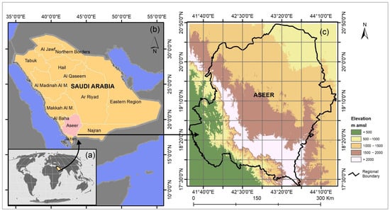
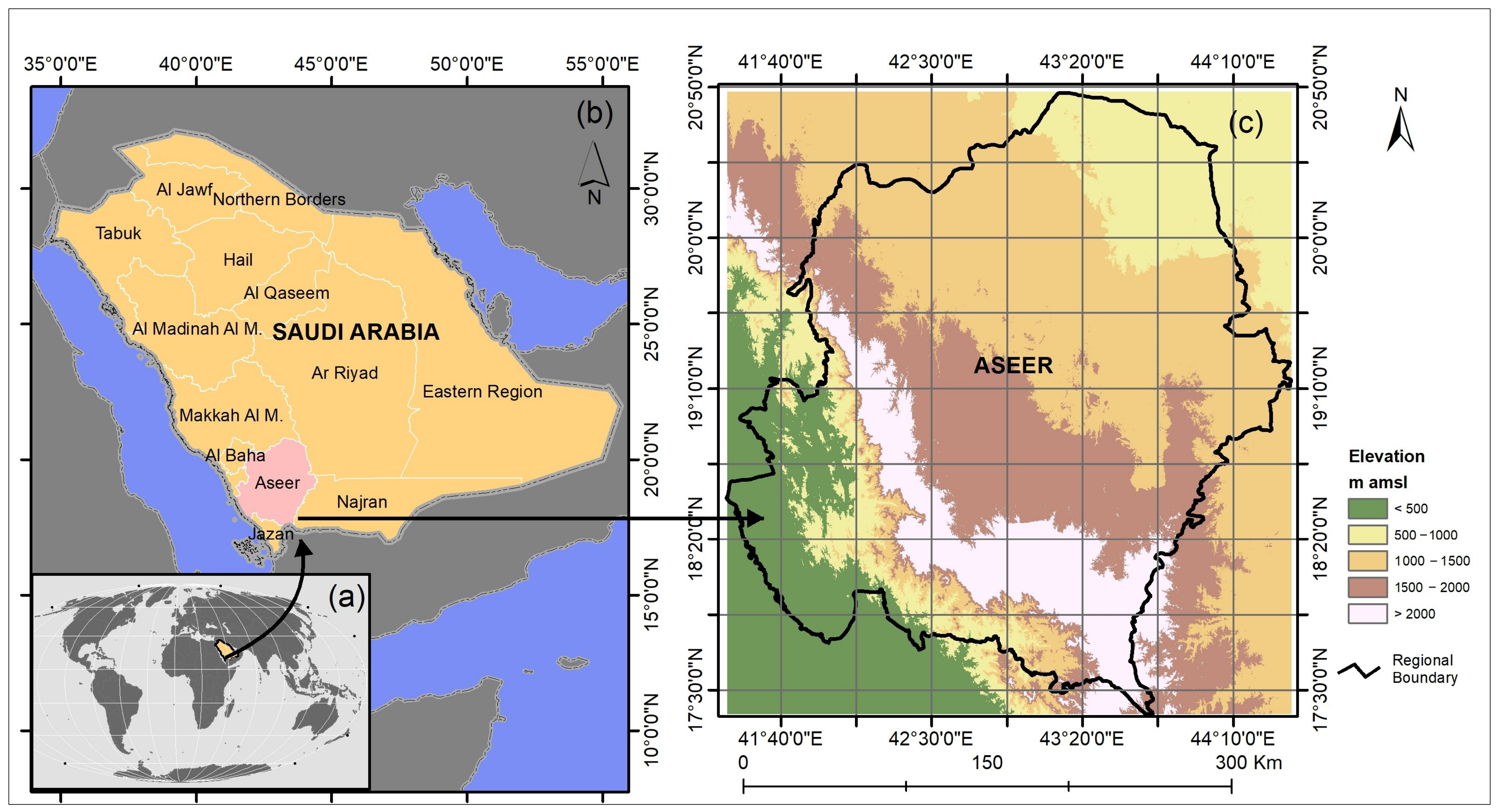
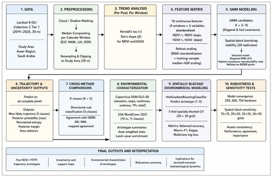
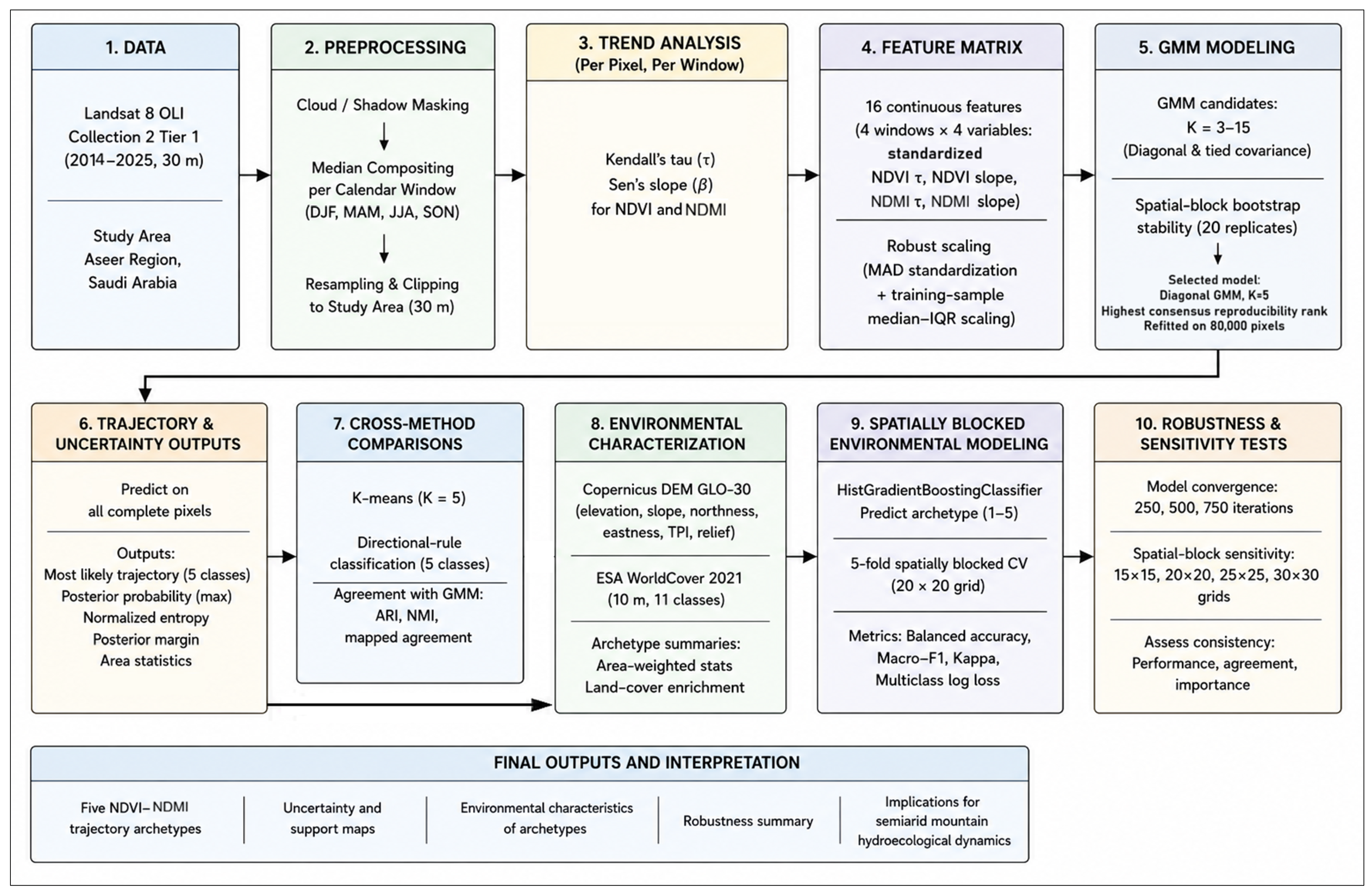
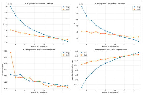
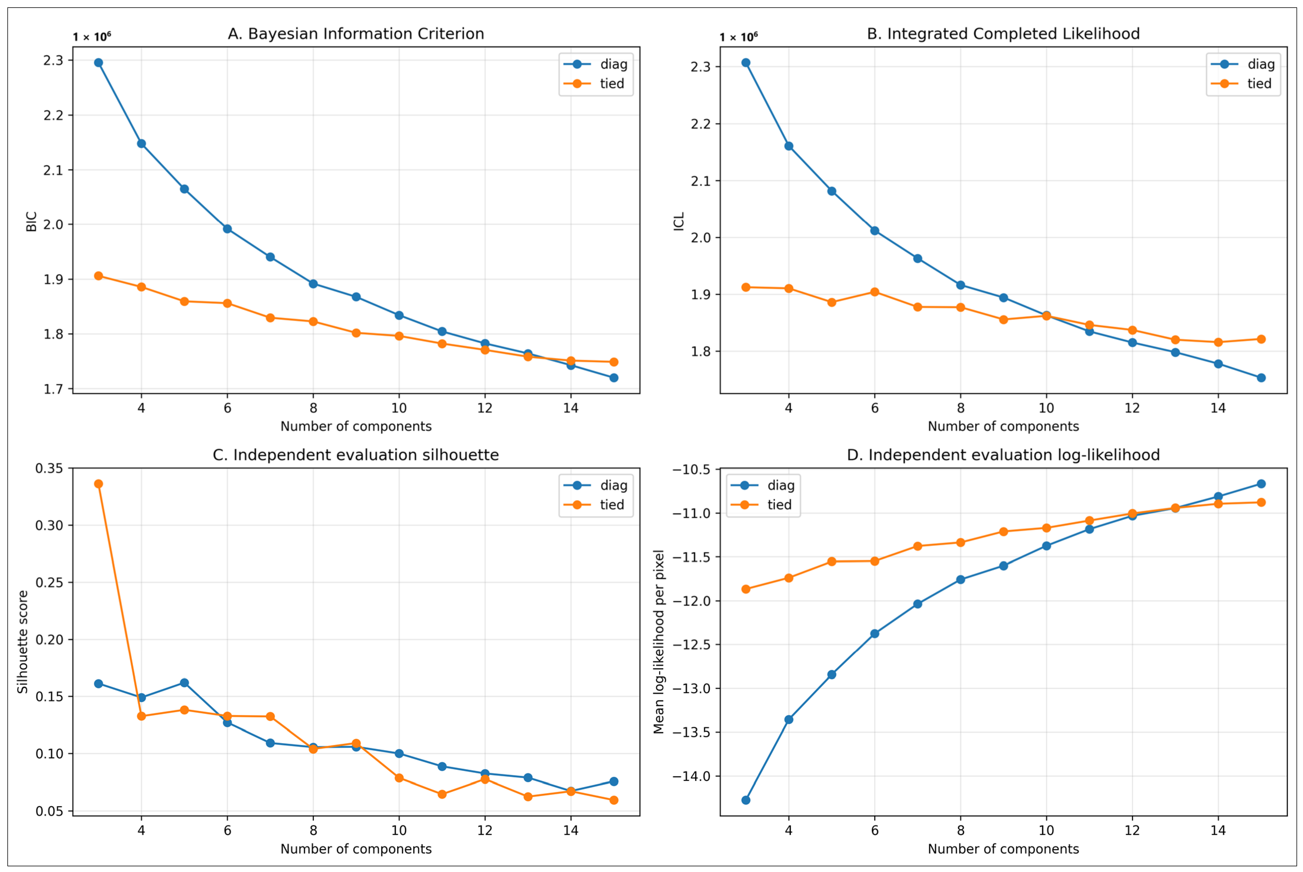
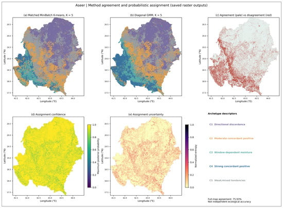
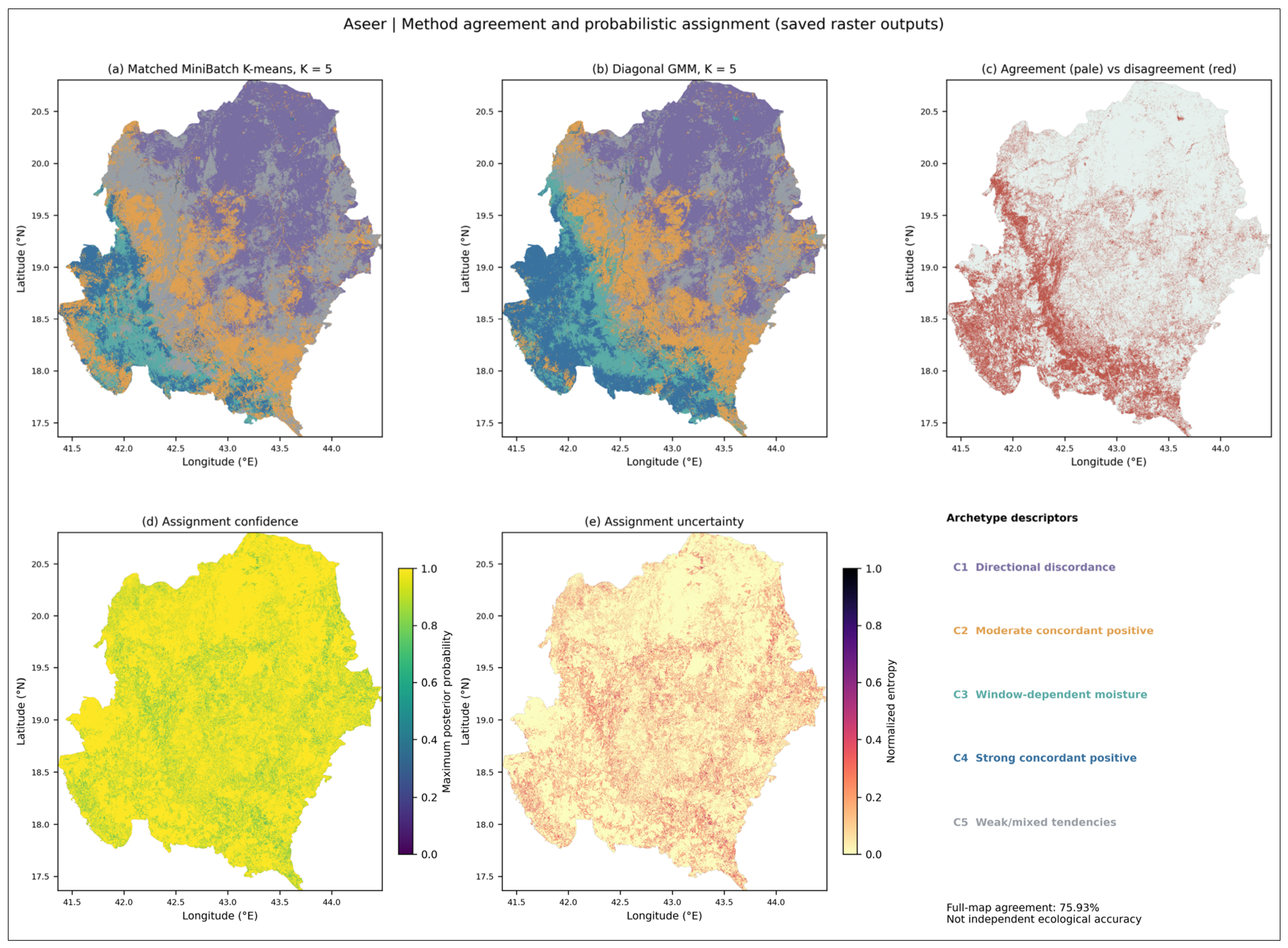
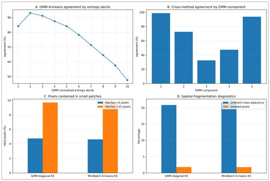
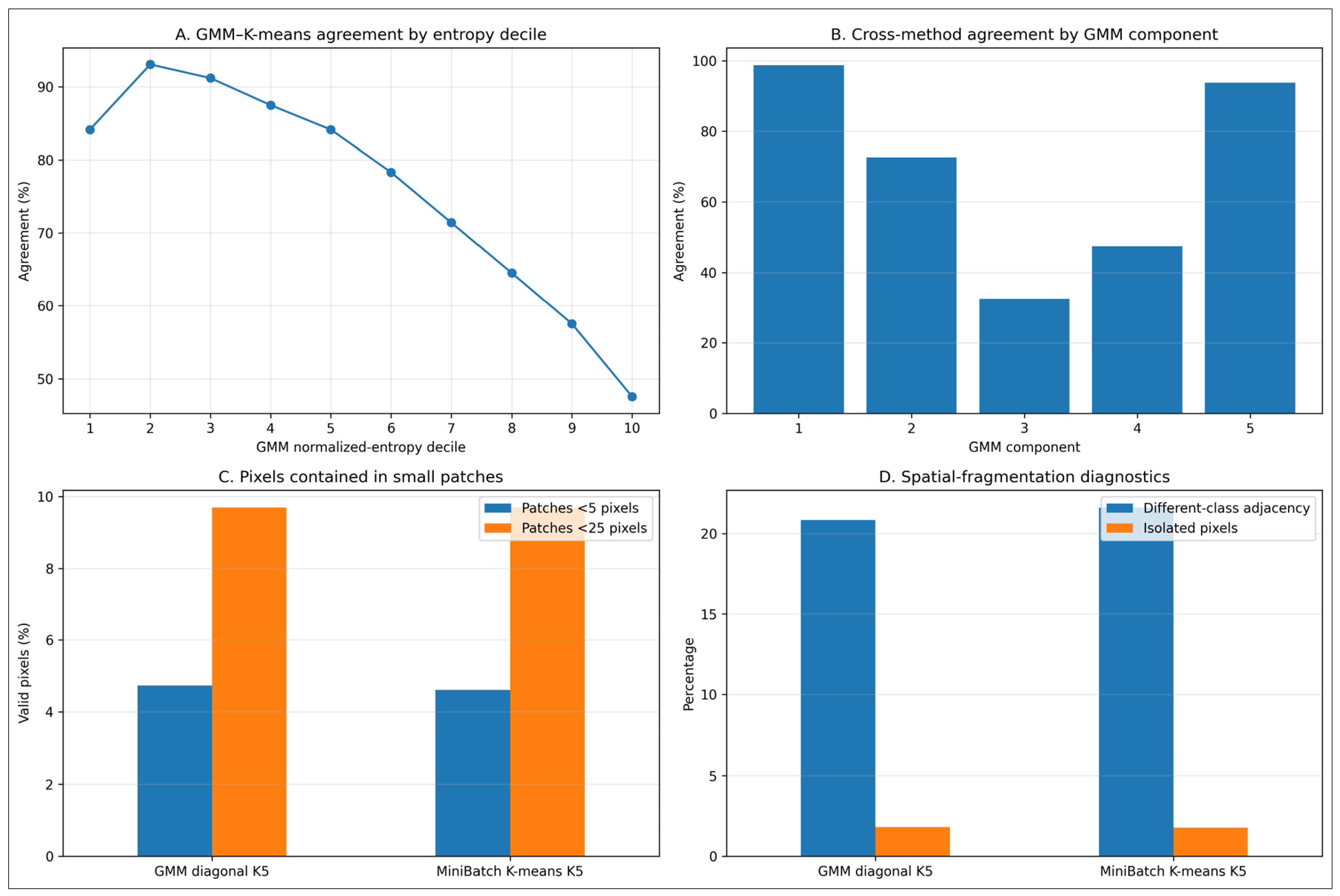
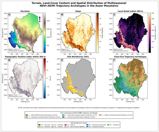
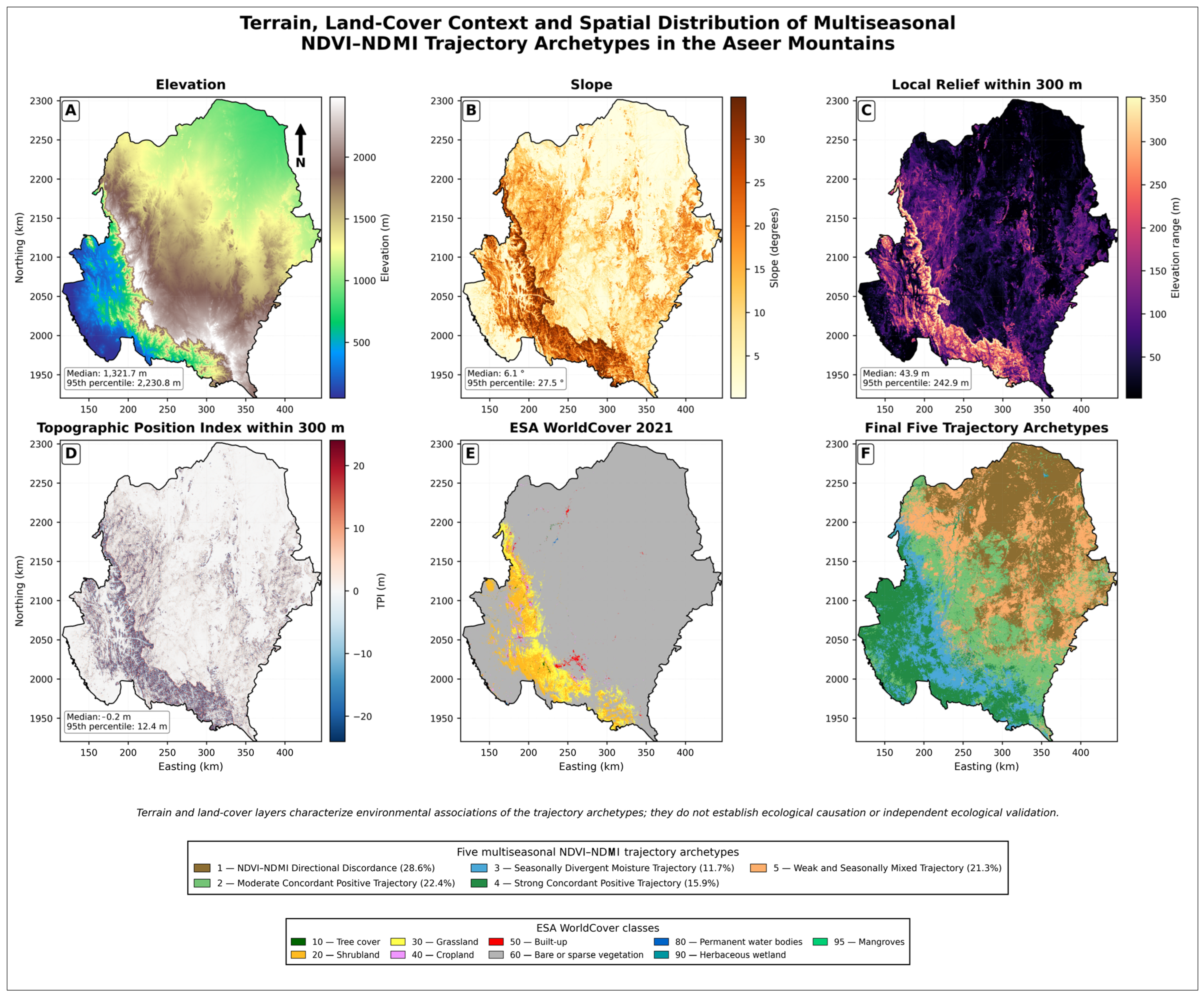
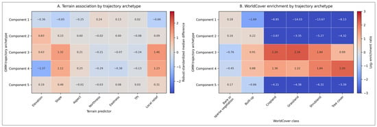
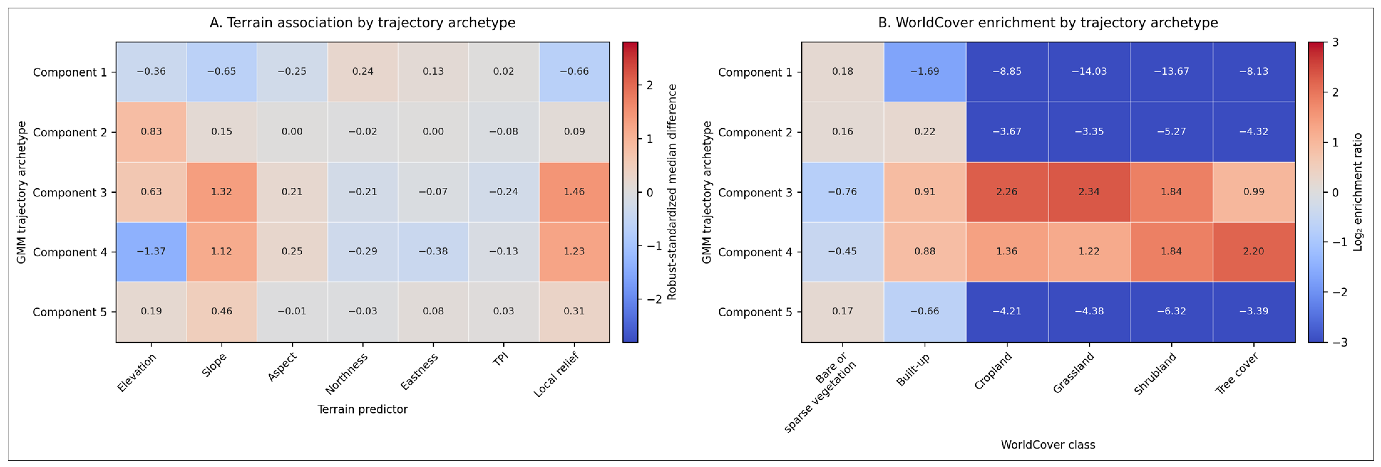
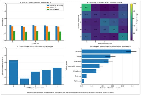
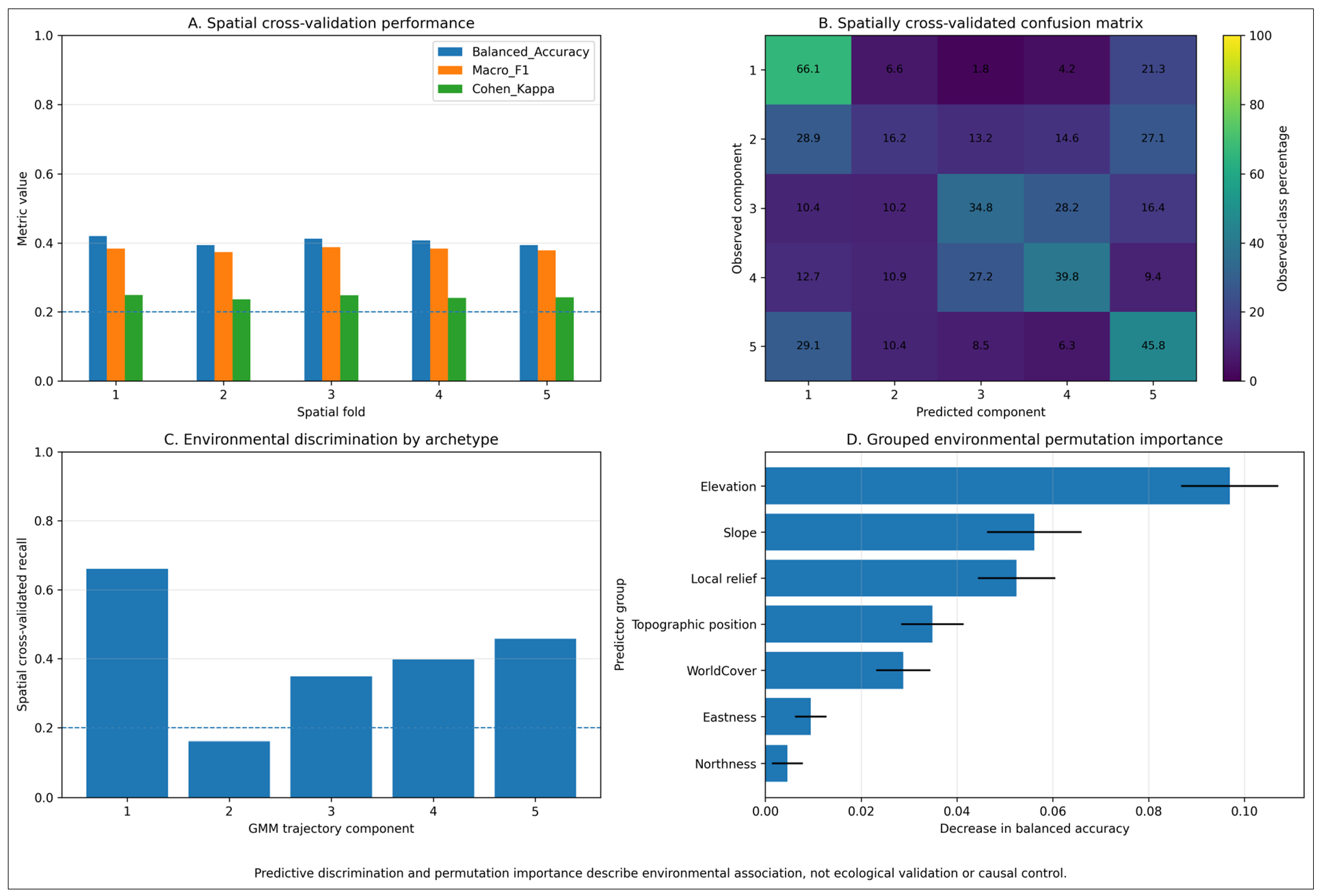

Disclaimer/Publisher’s Note: The statements, opinions and data contained in all publications are solely those of the individual author(s) and contributor(s) and not of MDPI and/or the editor(s). MDPI and/or the editor(s) disclaim responsibility for any injury to people or property resulting from any ideas, methods, instructions or products referred to in the content. |
© 2026 by the authors. Licensee MDPI, Basel, Switzerland. This article is an open access article distributed under the terms and conditions of the Creative Commons Attribution (CC BY) license.