


Highlights
What are the main findings?
- A coupling-embedded index distinguished provinces with similar baseline sustainability scores but contrasting Coupling Coordination Degree (CCD) values.
- MOSAIKS-inspired daytime remote-sensing features and nighttime lights recovered broad CESDI gradients in provinces excluded from model training (R2 = 0.4471), while within-province variation increased in 21 of 26 multi-unit provinces.
What are the implications of the main findings?
- Remote-sensing downscaling can extend long-term provincial sustainability assessments into an exploratory city-level screening layer where consistent local statistics are unavailable.
- Combining provincial CESDI, model-predicted within-province heterogeneity, and spatial clustering supports spatially targeted verification and differentiated sustainability monitoring, although individual-unit assessments require validation with data collected at the same administrative scale.
Abstract
Existing environmentally adjusted development indices can assign similar scores to regions with contrasting environmental–social configurations, while provincial averages conceal subprovincial variation. We developed a Coupling-Embedded Sustainable Development Index (CESDI), which retains the Sustainable Development Index (SDI) as baseline performance while incorporating an adjustment for the joint balance and overall development level of the environmental and social subsystems. CESDI was applied to 30 Chinese provincial-level units from 2002 to 2022. Exploratory predictions for 337 Chinese cities were generated using MOSAIKS-inspired Landsat features, nighttime lights, and dual-penalty ridge regression. CESDI preserved the interprovincial SDI gradient (Pearson r = 0.870 to 0.995) while differentiating provinces with similar SDI values but contrasting joint environmental–social conditions. National mean CESDI increased from 0.248 in 2002 to 0.465 in 2017 and declined to 0.371 in 2022. Nested province-grouped cross-validation yielded R2 = 0.4471 and RMSE = 0.1388. Feature-block ablation showed that the dual-penalty model outperformed daytime-only, nighttime-light-only, and equal-penalty specifications. The predicted share of high and very high classes increased from 12.5% to 37.1%, while within-province heterogeneity rose in 21 of 26 multi-unit provinces. The framework integrates baseline sustainability performance with a CCD-defined balance-and-level adjustment and provides an exploratory spatial-screening layer for identifying within-province variation.
1. Introduction
The United Nations 2030 Agenda frames social progress, economic development, and environmental protection as interdependent dimensions of sustainable development [1]. Monitoring progress toward the Sustainable Development Goals (SDGs) accordingly requires moving beyond global and national aggregates to identify spatial disparities in social development and environmental pressure at subnational scales [2,3,4,5]. The planetary boundaries framework delineates the biophysical thresholds within which Earth-system stability can be maintained [6,7,8], whereas the Safe and Just Operating Space complements these ecological limits with minimum social foundations, underscoring that ecological security and human well-being must advance jointly [9,10]. This integrated perspective is particularly relevant to China, where development stages, industrial structures, resource endowments, and environmental pressures vary markedly across provinces [11,12,13], and comparable levels of development can thus be associated with substantially different ecological costs and social shortfalls. Evaluating these outcomes within a consistent framework, while resolving disparities concealed by provincial aggregation, is critical for interpreting sustainability transitions and informing differentiated regional policies in a large and heterogeneous country [14,15].
Quantitative assessment that is both timely and comparable across regions is essential for evaluating regional sustainability and tracking its evolution [16,17]. Existing approaches follow two broad pathways. The first develops multidimensional indicator systems spanning economic, social, resource, and environmental domains [18]. Although such systems offer wide information coverage, discontinuous data, indicator selection, and weighting choices limit comparability across regions and over time [19,20,21,22,23]. The second incorporates environmental-pressure indicators, such as per capita carbon emissions, material footprints, or energy intensity, into the Human Development Index (HDI), enabling more parsimonious and temporally consistent assessments [24,25,26,27]. Despite their respective strengths, both pathways compress multidimensional information into a single score, meaning that similar index values may represent different combinations of environmental performance and social well-being [28,29]. Consequently, aggregate scores alone do not reveal whether these two subsystems develop in a coordinated manner or require different forms of policy attention.
Within the second pathway, Hickel [30] developed the Sustainable Development Index (SDI) by incorporating ecological overshoot into the HDI framework. Rather than treating human development alone as evidence of sustainability, SDI evaluates development achievements relative to the environmental pressures they entail. High human development accompanied by substantial ecological overshoot is accordingly not classified as strong sustainability performance. Application of SDI to 163 countries demonstrated the value of a consistent metric for large-scale and long-term comparison, while its parsimonious structure, transparent thresholds, and limited data requirements make it a transferable foundation for regional sustainability assessment.
Aggregate sustainability performance and environment–society coordination, however, capture different properties of regional development. SDI assesses human development relative to environmental pressure but does not directly reveal whether environmental performance and social well-being advance in a balanced manner. Similar SDI values do not imply similar environment-society configurations: one province may maintain balanced performance across the two subsystems, while another obtains the same aggregate score through the strength of a single subsystem. The Coupling Coordination Degree (CCD) provides an operational measure of the relative balance and joint development of multiple subsystems [4,31]. As a diagnostic indicator of numerical balance rather than evidence of causal interaction, CCD has generally been applied after composite indices have been calculated to explain observed differences [32,33]. Although informative, this post hoc treatment does not incorporate the joint subsystem state represented by CCD into the index calculation itself. Incorporating CCD directly into the SDI aggregation process allows the combined balance and overall development level of the environmental and social subsystems to adjust the SDI baseline retained in the final score. Through this adjustment, CESDI retains the baseline sustainability gradient captured by SDI while incorporating the CCD-defined subsystem configuration into the final score.
Beyond aggregation rules, sustainability diagnoses are also sensitive to the spatial scale at which indicators are constructed. Provincial statistics are relatively standardized and temporally continuous, making them suitable for long-term monitoring and broad regional comparison. Provincial averages, however, combine core cities, resource-dependent cities, and peripheral areas within a single observation, thereby obscuring substantial within-province variation through the modifiable areal unit problem [34,35]. Finer-scale assessment is constrained by the limited availability and consistency of long-term socio-ecological statistics. Remote sensing offers a practical means of narrowing this data gap: daytime imagery captures vegetation, land cover, and built-environment characteristics, whereas nighttime lights reflect the spatial intensity of human activity, infrastructure, and economic development. Both data sources have been widely used to estimate socioeconomic conditions at fine spatial scales [36,37,38], and advances in general-purpose remote-sensing feature learning have further improved the feasibility of spatial prediction when labeled observations are limited [39,40]. These developments provide a technical basis for extending provincial assessment into spatially explicit screening that reveals heterogeneity hidden by administrative averages. Taken together, existing assessments remain limited in their ability to differentiate regions with similar baseline sustainability performance but different joint environmental–social conditions, while consistent long-term evidence remains concentrated at the provincial scale and therefore obscures within-province variation.
To address these two gaps, this study develops a Coupling-Embedded Sustainable Development Index (CESDI) that retains SDI as a measure of baseline sustainability performance while incorporating CCD as an adjustment reflecting the joint environmental–social state. The study then combines provincial panel data with remote-sensing downscaling to extend the assessment from long-term provincial comparison to exploratory city-level spatial screening. Using panel data for 30 Chinese provincial-level units from 2002 to 2022, we first examine whether CESDI preserves the broad sustainability gradient captured by SDI while distinguishing provinces with comparable SDI values but different CCD-defined balance-and-level configurations. We then characterize the long-term trajectories and spatial distribution of provincial-level CESDI. MOSAIKS-inspired daytime features and nighttime-light data are subsequently integrated through dual-penalty ridge regression to generate exploratory predictions for 337 Chinese cities. A within-province heterogeneity index (HET) quantifies disparities among the predicted units, and their spatial clustering is assessed through global and local Moran’s I statistics. By linking baseline sustainability performance, coordination adjustment, and within-province variation, the framework connects long-term provincial comparison with remote-sensing-supported exploratory spatial screening (Figure 1).
Figure 1.
Conceptual framework and multiscale analytical workflow of CESDI.
2. Materials and Methods
2.1. Study Area
This study covers 30 provincial-level administrative units in China during 2002–2022. The Tibet Autonomous Region, Hong Kong Special Administrative Region, Macao Special Administrative Region, and Taiwan were excluded because of limitations in data continuity and statistical comparability. At the finer spatial scale, the analysis comprises 337 fixed cities and equivalent administrative units, including prefecture-level cities, autonomous prefectures, prefectures, leagues, and the four provincial-level municipalities treated as complete analytical units. For consistency with common usage in the literature, these units are hereafter referred to collectively as cities, and “city-level” denotes this analytical scale rather than a single legal administrative category.
To maintain spatial comparability throughout the study period, level-2 administrative boundaries from the Global Administrative Areas database (GADM, version 4.1) were adopted as a fixed spatial reference. The boundary data are available from the GADM website (https://gadm.org/download_country.html, accessed on 15 March 2026). Daytime remote-sensing imagery, nighttime-light data, and gridded population data were clipped and spatially harmonized within this boundary system. Raster-derived variables were subsequently aggregated using gridded population weights. The resulting city-level estimates therefore refer to spatially fixed analytical units rather than administrative boundaries that varied from year to year. This procedure improves temporal comparability but does not reconstruct historical administrative configurations.
Regional comparisons follow the four-region classification adopted by the National Bureau of Statistics of China, which divides the country into eastern, central, western, and northeastern regions (Table 1). Because Tibet was excluded from the analysis, the western region contains 11 provincial-level units. Each city-level unit was assigned to the same region as its corresponding province, and this classification was held constant throughout 2002–2022.
Table 1.
Regional classification of the provincial-level units included in the study.
2.2. Data Sources and Preprocessing
Five categories of data were assembled for the analysis. First, socioeconomic indicators were obtained primarily from the Human Development Reports published by the United Nations Development Programme and from successive editions of the China Statistical Yearbook, China Energy Statistical Yearbook, China Statistical Yearbook on Environment, China Land and Resources Statistical Yearbook, China Rural Statistical Yearbook, China Forestry Statistical Yearbook, and China Fishery Statistical Yearbook. Second, carbon-emission data used to quantify environmental pressure were obtained from the Carbon Emission Accounts and Datasets (CEADs), while freshwater use, nitrogen and phosphorus inputs, and land use were compiled from the corresponding statistical yearbooks.
Third, daytime remote-sensing inputs consisted of annual RGB composites derived from the encoded surface-reflectance bands of Landsat Collection 2 Level-2. The annual composites were generated in Google Earth Enbine (Google LLC, Mountain View, CA, USA; https://earthengine.google.com/, accessed on 20 March 2026). Landsat 5 Thematic Mapper (TM) data were used for 2002–2011, and Landsat 8 Operational Land Imager (OLI) data for 2013–2022. The same cloud-masking, fixed-range transformation, annual compositing, and export procedures were applied to both sensors, placing the resulting inputs on a common numerical RGB scale without constituting physical radiometric harmonization. Because no consistent annual composite was generated for 2012, the corresponding daytime features were interpolated from the adjacent years. The image-processing and interpolation procedures are detailed in Supplementary Sections S1.1 and S1.2.
Fourth, three population datasets served distinct analytical purposes. Annual global and provincial population totals were used in the allocation of environmental boundaries, while gridded population data provided the weights for aggregating remote-sensing features. Global population totals were obtained from the “Population, total” indicator in the World Bank’s World Development Indicators database, and provincial totals were compiled from successive editions of the China Statistical Yearbook. Annual gridded population counts for 2002–2020 were obtained from the WorldPop unconstrained individual-country population-count product at an approximate spatial resolution of 100 m (https://hub.worldpop.org/). Because equivalent grids were unavailable for the final two study years, the 2020 population distribution was held constant for 2021 and 2022. Further information on gridded-population processing and the population-weighting sensitivity analysis is provided in Supplementary Section S1.4, while environmental-boundary allocation is detailed in Supplementary Section S2.1.
Finally, the nighttime-light dataset comprises an annual harmonized time series for 2002–2022. The product was developed and is maintained by Chen et al. [41] and is available at https://doi.org/10.7910/DVN/YGIVCD (accessed on 25 March 2026). The procedures used to preprocess and aggregate the nighttime-light data are described in Supplementary Section S1.5.
2.3. Indicator System and Threshold Scoring
The indicator system is based on the Safe and Just Operating Space framework, which evaluates sustainability in terms of both ecological limits and minimum social foundations [9,10,42]. The environmental subsystem assesses regional environmental footprints relative to the corresponding allocated boundaries, thereby indicating the extent to which environmental pressures remain within or exceed those limits. The social subsystem evaluates the degree to which basic social objectives are achieved. Indicators in the two subsystems are scored and aggregated separately to derive environmental performance and social well-being, respectively. These subsystem-level measures subsequently serve as inputs for calculating CCD and, through CCD, CESDI.
2.3.1. Environmental Performance
The environmental subsystem represents four of the nine Earth-system processes identified in the planetary boundaries framework using five indicators: carbon emissions, freshwater use, human-modified land area, nitrogen fertilizer application, and phosphorus fertilizer application (Table 2). These indicators were selected according to three criteria: their suitability for spatial allocation, the continuity of provincial data over 2002–2022, and the avoidance of substantial information overlap among indicators [6,7,8]. Stratospheric ozone depletion and atmospheric aerosol loading were excluded because their boundaries cannot be meaningfully allocated to individual provinces. Biosphere integrity and novel entities were omitted because consistent provincial time-series data were unavailable, and ocean acidification was not represented separately because its information content substantially overlaps with that of carbon emissions. This selection prioritizes indicators that can be allocated consistently across provinces and tracked over the full study period.
Table 2.
Environmental-pressure indicators, global control values, and data sources.
Carbon-related pressure enters the CESDI framework through two pathways: per capita carbon emissions contribute to the SDI baseline, and the carbon footprint forms part of the environmental subsystem. This design creates partial overlap in the carbon-related information incorporated into CESDI. To evaluate whether this overlap materially affects the results, the index was recalculated after excluding the carbon indicator from the environmental subsystem. The corresponding sensitivity analysis is reported in Supplementary Section S3.
Global planetary boundaries were allocated to the provincial scale according to the equal per capita principle [4,43]. The allocated ecological boundary (EB) for environmental indicator j in province i and year y was calculated as follows:
where EBi,j,y denotes the allocated ecological boundary for environmental indicator j in province i and year y; is the global boundary for indicator j; is the global population in year y; and Popi,y is the population of province i in year y. Equal per capita allocation provides a transparent and reproducible equal-entitlement benchmark, rather than an empirically determined or normatively unique distribution of provincial environmental space.
For climate change, equal per capita allocation was operationalized using year-specific per capita CO2 emissions limits following Han et al. [4]. Han et al. derived these annual limits from the remaining cumulative carbon budget associated with a 50% probability of limiting global warming to less than 2 °C above pre-industrial levels and the cumulative projected global population to 2100. The published limits declined from 1.70 t CO2 capita−1 yr−1 in 2002 to 1.29 t CO2 capita−1 yr−1 in 2018. For 2019–2022, we extended the series to 1.26, 1.23, 1.19, and 1.16 t CO2 capita−1 yr−1, respectively. Provincial climate-pressure ratios were calculated by dividing provincial per capita CO2 emissions by the corresponding annual limit.
The Environmental Pressure Ratio (EP) was calculated as the ratio of an environmental footprint to its corresponding allocated ecological boundary:
where EPi,j,y denotes the environmental pressure ratio for indicator j in province i and year y, and EFi,j,y is the corresponding environmental footprint. To standardize the direction and scale of the indicators, reverse min–max normalization was applied using fixed extrema calculated across all provinces and years:
where EPminj and EPmaxj are the minimum and maximum values, respectively, of indicator j across all provinces and years. Xij ∈ [0, 1], with higher values indicating better relative environmental performance. Supplementary Section S4 further examines the robustness of the results using a distance-to-target scoring method that preserves absolute threshold interpretation.
2.3.2. Social Well-Being
The social subsystem comprises ten dimensions: food security, income, drinking water, sanitation, health care, energy, education, gender equality, social equity, and employment. Each dimension is linked to a corresponding Sustainable Development Goal (SDG) and is represented by an operational indicator and threshold (Table 3). Threshold values were primarily derived from O’Neill et al. [42], Han et al. [4], and Chen et al. [11], with adjustments made according to the availability and comparability of provincial data in China. These thresholds provide a consistent reference for evaluating social well-being across provinces and over time. Threshold attainment is interpreted dimension by dimension, providing a consistent benchmark for comparing specific components of social well-being.
Table 3.
Social-foundation dimensions, SDG links, indicators, and diagnostic thresholds.
Social well-being (SW) was calculated as the degree to which each social indicator attained its corresponding threshold:
where SWi,j,y is the attainment level of social indicator j in province i and year y; SIi,j,y is the observed value of social indicator j in province i and year y; and STj is the social threshold for indicator j. The Gini coefficient was converted to percentage form before calculation.
To prevent performance above a threshold from providing additional compensation for deficits in other dimensions, each attainment score was capped at 1:
where Yi,j,y is the standardized score for social indicator j in province i and year y and ranges from 0 to 1.
Yi,j,y = min(SWi,j,y,1)
2.3.3. Subsystem Aggregation
Equal-weight arithmetic means were used within both the environmental and social subsystems to avoid assigning disproportionate influence to specific indicators without sufficient normative justification:
where f(x) and f(y) denote the aggregate performance of the environmental and social subsystems, respectively. Both range from 0 to 1, with values closer to 1 indicating better performance. After aggregation, the environmental and social subsystem scores were separately rescaled using min–max normalization across the complete panel of 630 province–year observations. The resulting normalized subsystem scores were used to calculate C and T. Accordingly, a normalized subsystem score of zero represents the lowest observed value within the study panel rather than the complete absence of environmental or social performance.
2.4. Construction of CESDI
Following Liang et al.’s [44] provincial implementation of Hickel’s [30] Sustainable Development Index framework, the SDI baseline was constructed using provincial human-development indicators, per capita carbon emissions, and domestic material consumption. A CCD-based adjustment was then introduced to derive CESDI:
CESDI = SDI × P
The detailed calculation of SDI is provided in Supplementary Section S5. P is the adjustment term, ranging from 0 to 1, and its baseline formulation is defined as follows:
where CCD is the Coupling Coordination Degree, ranging from 0 to 1, and is calculated as follows:
where C measures the relative balance between environmental performance and social well-being and ranges from 0 to 1. A higher C value indicates greater numerical balance between the two subsystems, whereas a lower value indicates greater imbalance. C is used as a structural balance measure between the environmental and social subsystems. T represents their overall development level. Because CCD is jointly determined by C and T, a lower CCD may result from greater relative imbalance, a lower overall level of the two subsystems, or both. CCD is therefore interpreted as a joint balance-and-level measure rather than as a pure measure of environment–society imbalance. In this study, CCD is a descriptive index derived algebraically from contemporaneous subsystem scores. It summarizes their numerical balance and joint development level but does not estimate causal effects, feedback processes, or the direction of influence between the environmental and social subsystems. In the following equations, f(x) and f(y) refer to the environmental and social subsystem scores after the post-aggregation min–max normalization described in Section 2.3.3. C and T are calculated as follows:
where α and β are the weights assigned to the environmental and social subsystems, respectively, with α + β = 1. Following [4], equal weights were assigned to the two subsystems (α = β = 0.5).
P = CCD
To identify the sources of the post-2017 change in CESDI, the change between 2017 and 2022 was decomposed symmetrically into SDI and CCD components. The SDI component was calculated as the change in SDI multiplied by the mean CCD of the two years, whereas the CCD component was calculated as the change in CCD multiplied by the mean SDI. The two components sum exactly to the total change in CESDI.
2.5. Index Behavior and Internal Consistency
2.5.1. Correlation and Matched-Pair Comparison
To examine whether CESDI preserves the baseline sustainability information represented by SDI, Pearson correlation coefficients between the two indices were calculated for 2002, 2012, and 2022. For each representative year, the province pair with the smallest absolute difference in SDI was identified. Differences in their CCD and CESDI values were then compared to determine whether the CCD-based adjustment differentiated provinces with otherwise similar baseline performance. The selected pairs are highlighted in Figure 2 and summarized in Table 4. A within-year pairwise analysis was additionally conducted to identify similar CESDI values arising from contrasting SDI and CCD configurations; the definitions and threshold-sensitivity tests are provided in Supplementary Section S6.3. To assess sensitivity to the two zero-CESDI observations arising when a post-aggregation normalized subsystem score reached the panel lower boundary, we conducted leave-one-out checks and a positive-floor test in which zero-valued SDI and/or CCD terms were replaced with the smallest positive values observed in the panel. Changes in annual means, within-year provincial rankings, and SDI–CESDI correlations were then evaluated.
Figure 2.
Provincial-level relationships between SDI and CESDI in 2002, 2012, and 2022. The diagonal is the 1:1 line, and colors represent CCD on a common 0–1 scale. Red labels show the province pair with the smallest within-year SDI difference, with ∆CESDI indicating the corresponding absolute CESDI difference. Guizhou’s 2002 zero observation is shown at the origin and included in Pearson’s r. *** p < 0.001.
Table 4.
Matched-province comparisons illustrating the differentiation introduced by the CCD-based adjustment.
2.5.2. Internal Robustness
To assess the structural robustness of CESDI, we recalculated the index using alternative aggregation functions and environmental–social weighting schemes. The complete formulations and corresponding sensitivity results are reported in Supplementary Section S6.
2.6. Remote-Sensing Downscaling
2.6.1. MOSAIKS-Inspired Daytime Features
To obtain general-purpose spatial representations for cross-scale prediction, fixed random-convolution features were extracted from annual Landsat red–green–blue (RGB) composites following the MOSAIKS framework [36,39]. The annual composites were generated at a spatial resolution of 100 m and partitioned into non-overlapping windows of 10 × 10 pixels, corresponding to analytical units of approximately 1 km × 1 km. Each three-channel image window was passed sequentially through random convolution, rectified linear unit (ReLU) activation, and global average pooling. This procedure produced a 4000-dimensional daytime feature vector for each analytical unit:
where Xday is the 4000-dimensional daytime feature vector for the grid cell; Pool(⋅) denotes global average pooling over the spatial dimensions; ReLU(⋅) is the rectified linear unit activation function; and W and b are the randomly generated and fixed convolution-kernel weights and biases, respectively.
Xday = Pool(ReLU(W ⋅ xday+b))
2.6.2. Nighttime-Light Features
Nighttime-light data were incorporated to capture dimensions of human activity and infrastructure that are not directly represented by daytime imagery. Administrative-unit mean radiance was not used directly because the radiance distribution was zero-inflated, strongly right-skewed, and characterized by a long upper tail. Instead, temporally consistent binned features were constructed [40]. All zero-radiance observations among valid grid cells during 2002–2022 were assigned to a separate no-light class. Positive radiance values were pooled across the entire study period and divided into 20 quantile-based intervals, yielding 21 classes in total. The resulting class boundaries were fixed across years and applied identically when aggregating nighttime-light features at the provincial and city-level scales. This design preserved temporal and cross-scale comparability while reducing the influence of extreme radiance values.
For administrative unit c, the nighttime-light feature vector was calculated as follows:
where is the 21-dimensional nighttime-light feature vector for administrative unit c, and its kth element represents the proportion of the unit’s resident population located in grid cells whose radiance falls within bin k. Here, c denotes an administrative unit, either a province or a city-level unit; i denotes a 1 km grid cell within unit c; Popi is the population of grid cell i, obtained from the gridded-population data for year y; bink denotes the radiance interval covered by bin k, where (k = 1, 2, …, K); and c ∩ bink is the set of grid cells located within administrative unit c whose radiance values fall in bink.
Accordingly, the daytime and nighttime-light feature blocks represent observable surface and illumination patterns rather than direct measurements of environmental performance, social well-being, or CESDI.
2.6.3. Ridge Regression Model and Validation
The 4000-dimensional daytime feature vector and the 21-dimensional nighttime-light feature vector were concatenated to produce a 4021-dimensional joint representation for each province–year observation. The corresponding CESDI values for 30 provincial-level units over 2002–2022 provided 630 province–year training targets. To accommodate the substantial difference in dimensionality between the two feature groups and permit group-specific shrinkage, a dual-penalty ridge regression model was employed rather than imposing a single regularization parameter on all predictors. Separate L2 penalties were therefore applied to the coefficients of the daytime and nighttime-light feature groups. The model was estimated by minimizing the following objective function:
where L is the objective function; and are the provincial daytime and nighttime-light feature vectors, respectively, for province p in year y; P and Y are the total numbers of provinces and years; CESDIp,y is the coupling-embedded sustainable development index for province p in year y; βday, βntl and β0 are the model parameters; and λday and λntl control the shrinkage applied to the two coefficient groups.
To determine whether the full model provided predictive information beyond temporal and feature-based baselines, five specifications were compared: (1) a year-mean baseline, which assigned each held-out province the mean CESDI of the corresponding year calculated from the outer-training provinces; (2) a nighttime-light-only ridge model; (3) a daytime-feature-only ridge model; (4) an equal-penalty model combining both feature blocks under a single ridge penalty; and (5) the full dual-penalty model. All specifications used the same outer province-grouped folds, while feature centering and penalty selection for the ridge models were performed exclusively within the corresponding training data.
Model performance was evaluated using a 5 × 5 nested GroupKFold cross-validation design, with provinces defined as the grouping units. All annual observations from a given province were assigned to the same fold, allowing the validation procedure to assess spatial generalization to provinces not represented in model training. The five outer folds generated out-of-fold predictions for held-out provinces, whereas the five inner folds were restricted to the corresponding outer-training set and used to select the relative weight assigned to the daytime features and the base ridge penalty, which together determined the two group-specific penalties. Feature-centering parameters were estimated exclusively from the training data within each fold and then applied to the corresponding validation data. Hyperparameters were likewise selected using only the training folds, preventing validation-fold information from entering feature centering or hyperparameter selection.
All baseline, ablation, and full models were evaluated using the same outer province-grouped folds. Feature transformation and ridge-penalty selection were performed exclusively within the corresponding training data. Performance was evaluated from the pooled outer-fold predictions using R2, RMSE, MAE, Pearson’s r, mean bias, and the calibration slope obtained by regressing predicted values on observed CESDI. Full implementation details are provided in Supplementary Section S7.
After nested cross-validation had been used to estimate out-of-sample performance, deployment hyperparameters were reselected using all 630 province–year observations, and the final dual-penalty ridge regression model was refitted to the complete provincial training dataset. The city-level predictor matrix was constructed using the same feature definitions, population-weighted aggregation procedures, and column order as the provincial training matrix. City-level features were then centered using the parameters estimated from the complete provincial sample and entered into the fitted model to generate exploratory city-level CESDI predictions:
where CESDIc,y is the predicted CESDI for unit c in year y; is the population-weighted mean joint feature vector for unit c in year y; and and are the coefficient and intercept estimates obtained from the provincial ridge regression model. In the absence of a consistent national city-level CESDI benchmark, the fitted model projected relationships estimated from provincial data onto fixed city-level units to produce an exploratory spatial-screening layer.
2.7. Multiscale Spatial Diagnostics
2.7.1. Provincial Trend Estimation
Long-term changes in provincial-level CESDI over 2002–2022 were quantified using ordinary least squares (OLS) regression. For each province, CESDI was regressed on time using the complete 21-year series, and the estimated slope was interpreted as the mean annual linear change in CESDI over the study period [45]. Because annual observations may exhibit temporal autocorrelation, the standard errors, 95% confidence intervals, and two-sided p-values of the provincial OLS trends were calculated using the Newey–West heteroskedasticity- and autocorrelation-consistent covariance estimator with a maximum lag of two years:
where CESDIp,y is the observed provincial-level CESDI for province p in year y; βp is the province-specific intercept, representing the estimated CESDI value in 2002; θp is the OLS temporal-trend coefficient, representing the mean annual linear change in CESDI over the study period, with units of CESDI units yr−1; and εp,y is the random error term. The OLS slope was retained as the estimate of the mean annual linear change, while statistical significance was evaluated using the HAC-adjusted standard error.
CESDIp,y = βp + θp(y-2002) + εp,y
2.7.2. Within-Province Heterogeneity Index
To quantify within-province variation obscured by provincial averages, the within-province heterogeneity index (HET) was defined as the population-weighted standard deviation of predicted CESDI across cities. HET measures the dispersion of unit-level predictions around the corresponding provincial population-weighted mean. For province p in year y, the population-weighted mean CESDI across all valid constituent units was calculated as follows:
where CESDIp,y′ is the population-weighted mean of predicted city-level CESDI for province p in year y. HET was then calculated as follows:
where HETp,y is the within-province heterogeneity of province p in year y. HET describes within-province variation in the predicted CESDI surface and does not indicate the province’s overall level of sustainable development.
2.7.3. Spatial Autocorrelation
Global and local Moran’s I statistics were calculated for five representative years (2002, 2007, 2012, 2017, and 2022) to characterize the spatial clustering and temporal evolution of predicted city-level CESDI across China from 2002 to 2022 [46]. Global Moran’s I measures the direction and strength of overall spatial autocorrelation in the national predicted surface, whereas local Moran’s I identifies localized concentrations of similar or dissimilar predicted values. These statistics characterize the spatial organization of predicted CESDI under the specified spatial-weight matrix. The global and local indices were calculated as follows:
Higher Moran’s I values indicate stronger positive spatial autocorrelation, whereas lower values indicate greater spatial dispersion; statistical significance was assessed as described in Supplementary Section S8. n is the number of cities in the study area; Yi and Yj are the predicted CESDI values for units i and j, respectively; is the national mean predicted city-level CESDI; S2 is the sample variance of the predicted CESDI values; and Wij is the spatial-weight matrix. First-order Queen contiguity was defined using binary adjacency weights, such that Wij = 1 when units i and j share a boundary or vertex and Wij = 0 otherwise. The resulting weights were row standardized for analysis. Implementation settings and annual significance thresholds [47] are provided in Supplementary Section S8.
3. Results
3.1. Index Performance
CESDI preserved the principal interprovincial gradient captured by SDI while providing additional differentiation among provinces with nearly identical baseline scores. Pearson correlations between provincial-level CESDI and SDI were 0.870 in 2002, 0.982 in 2012, and 0.995 in 2022, indicating strong consistency between the two indices (Figure 2). The highlighted matched pairs nevertheless occupied visibly different CESDI positions because of their contrasting CCD values. In 2002, Hunan and Ningxia differed by only 0.003 in SDI but by 0.337 in CCD, resulting in CESDI values of 0.212 and 0.076, respectively. The Zhejiang–Henan pair in 2012 had absolute differences of 0.002 in SDI, 0.122 in CCD, and 0.063 in CESDI. In 2022, the corresponding differences between Shandong and Heilongjiang were 0.003, 0.271, and 0.077, respectively (Table 4). These comparisons demonstrate that provinces occupying nearly identical positions under SDI can be differentiated when their joint environmental–social conditions are incorporated. The broader pairwise analysis further identified contrasting SDI–CCD configurations in 93 of the 288 pairs with similar CESDI values, representing 32.29% of the similar-CESDI pairs and 1.02% of all 9135 within-year comparisons (Supplementary Section S6.3).
3.2. Provincial-Level CESDI
3.2.1. Temporal Evolution
From 2002 to 2022, CESDI exhibited a net increase, with a pronounced rise until 2017 followed by a decline (Figure 3a). The national mean provincial-level CESDI increased from 0.248 in 2002 to a peak of 0.465 in 2017 and subsequently declined to 0.371 in 2022, remaining 0.123 above the 2002 level. Under the two-factor accounting decomposition, 0.0939 of the 0.0940 reduction in national mean CESDI was assigned to changes in the SDI component and 0.0001 to changes in the CCD component. The SDI component also accounted for the larger absolute share of the decline in 24 of the 25 provinces with decreasing CESDI. All four regions reached local peaks in 2017, but their long-term changes differed markedly. Eastern China maintained the highest level, increasing from 0.384 to 0.482. Central China recorded the largest net increase, rising by 0.202 from 0.215 to 0.417, while western China increased by 0.148 from 0.124 to 0.272. Northeastern China was the only region to show a net decline, decreasing by 0.042 from 0.319 to 0.276. By 2022, the gap between eastern and central China had narrowed from 0.169 to 0.065, indicating a marked convergence of central China toward the eastern region over the study period.
Figure 3.
Provincial-level CESDI dynamics in China from 2002 to 2022. (a) Annual mean CESDI trajectories for China and the four geographical regions. (b) Province–year heatmap of CESDI. (c) Provincial-level OLS average annual changes, with 95% confidence intervals calculated using Newey–West heteroskedasticity- and autocorrelation-consistent standard errors with a maximum lag of two years. Filled and open circles indicate trends with HAC-adjusted two-sided p < 0.05 and p ≥ 0.05, respectively.
The province–year heatmap revealed substantial interprovincial divergence behind these regional averages (Figure 3b). Within eastern China, Beijing, Shanghai, and Guangdong remained at relatively high levels, whereas Shandong declined from 0.317 to 0.250. The overall increase in central China was concentrated mainly in Hunan, Jiangxi, and Henan, while Shanxi declined to 0.012. Sichuan, Chongqing, and Yunnan increased markedly in western China, whereas Xinjiang, Shaanxi, and Ningxia remained at relatively low levels in 2022. Northeastern China also diverged internally: Jilin increased to 0.454, while Liaoning and Heilongjiang declined to 0.201 and 0.173, respectively.
Provincial-level OLS trend coefficients demonstrated substantial variation in long-term CESDI change (Figure 3c). Based on Newey–West HAC standard errors, 16 of the 30 provinces exhibited significant increasing trends, seven exhibited significant decreasing trends, and the remaining seven showed no statistically significant linear change (p ≥ 0.05). Sichuan, Hunan, and Chongqing had the fastest increases, with trend coefficients of 23.59 × 10⁻³, 21.24 × 10⁻³, and 20.91 × 10⁻³ CESDI units yr−1, respectively; Beijing, Jiangxi, and Yunnan also showed pronounced significant increases. In contrast, Xinjiang, Inner Mongolia, and Shanxi recorded the largest declines, with coefficients of −14.63 × 10⁻³, −9.76 × 10⁻³, and −9.65 × 10⁻³ CESDI units yr−1, respectively. Additional checks broadly supported the direction of the estimated trends: a one-year HAC lag produced the same classification for 29 of the 30 provinces, and a Prais–Winsten AR(1) specification retained the trend direction for 27 provinces, with all three direction changes occurring among nonsignificant trends.
The provincial CESDI trajectories shown in Figure 3 were calculated entirely from statistical indicators and are therefore independent of the Landsat and gridded-population inputs, which were used only in the city-level downscaling analysis.
3.2.2. Spatial Patterns
To characterize the spatial expression of these temporal changes, provincial-level CESDI distributions were compared across five representative years (Figure 4). The spatial pattern shifted from an early advantage concentrated along the eastern coast to the coexistence of persistent coastal high values and localized improvements in central and western China. In 2002, the highest values were concentrated in Shanghai, Beijing, Zhejiang, Tianjin, and Jiangsu, whereas CESDI remained below 0.15 in Gansu, Ningxia, Yunnan, Sichuan, and Qinghai. After 2012, improvements became more spatially dispersed, and the medium-to-high-value zone extended from the eastern coast toward the middle reaches of the Yangtze River and southwestern China. By 2022, Beijing and Shanghai remained among the leading provinces, while CESDI exceeded 0.58 in Guangdong, Hunan, Sichuan, Jiangxi, and Chongqing, indicating that high values were no longer restricted to the traditional eastern core. In contrast, Shanxi, Xinjiang, Ningxia, and Shaanxi remained in the low-value group. Northeastern China also exhibited pronounced internal differences in 2022: CESDI reached 0.454 in Jilin but only 0.201 in Liaoning and 0.173 in Heilongjiang. The resulting spatial pattern combined a persistent eastern advantage with localized gains in central and southwestern China and continued low values across northwestern China and parts of the northeast.
Figure 4.
Spatial distribution of provincial-level CESDI in representative years.
3.3. Downscaled CESDI Predictions
3.3.1. Downscaling Performance
Predictive performance improved as the two remote-sensing feature blocks were combined and separately regularized. Under the same province-grouped validation design, R2 was −0.0451 for the year-mean baseline, 0.2466 for the nighttime-light-only model, 0.0802 for the daytime-feature-only model, 0.3953 for the equal-penalty model, and 0.4471 for the dual-penalty model (Figure 5b). The full model achieved an RMSE of 0.1388 and an MAE of 0.1148 (Figure 5a; Supplementary Table S13).
Figure 5.
Out-of-province predictive performance of the CESDI downscaling model. (a) Observed versus out-of-fold predicted CESDI from the selected dual-penalty model for 630 province–year observations under five-fold GroupKFold by province. The solid line is the fitted regression, and the dashed line is the 1:1 reference. (b) Out-of-fold R2 and RMSE for the selected model and four comparator models; higher R2 and lower RMSE indicate better performance.
The calibration slope of 0.4908 was associated with overprediction at the lower end and underprediction at the upper end of the observed CESDI distribution. Transition-period sensitivity tests showed that excluding 2012 or 2012–2013 had little effect on pooled out-of-province performance and that the nighttime-light-only model produced a larger 2011–2013 increase than the daytime-feature-only model, although prediction error was higher in 2013 (Supplementary Table S2). Because the harmonized nighttime-light series also spans a change in source sensors around this period [41], part of this increase may reflect residual cross-sensor inconsistency rather than actual change.
Reaggregating the city-level estimates to the provincial scale produced a mean residual of 0.0041 relative to the provincial predictions from the same model, with 98.41% of absolute residuals below 0.05; the larger deviations occurred mainly among low-CESDI observations (Supplementary Table S13).
3.3.2. Predicted CESDI Distribution Across Chinese Cities
Predicted CESDI values for the 337 cities during 2002–2022 were classified into five levels using the Jenks natural breaks method. The breakpoints were estimated once from the pooled city-level predictions and held constant across all years, allowing prediction patterns and class compositions to be compared across five representative years (Figure 6). The predicted surface shifted from a predominance of very low and low values toward an expansion of high and very high values, although regional gradients persisted (Figure 6a). In 2002, units in the very low and low classes were concentrated primarily in northwestern China and parts of northern China, whereas units in the high and very high classes were scattered along the eastern coast and across southern China. From 2007 onward, high and very high values gradually extended into central and southwestern China. By 2017 and 2022, relatively dense concentrations of the high and very high classes had formed along the eastern coast and across central and southwestern China. Contiguous low-value areas, by contrast, persisted in northwestern China and parts of northeastern China. The predicted surface thus exhibited a broad upward class transition without eliminating the underlying spatial gradient.
Figure 6.
Predicted city-level CESDI distribution. (a) Spatial distribution of city-level CESDI predictions in five representative years. (b) Proportions of cities across the five predicted CESDI classes in the corresponding years. Note that the 2012 predictions combine interpolated Landsat-derived daytime features with contemporaneous nighttime-light data.
Under the fixed classification thresholds, the distribution of city-level CESDI predictions shifted toward higher classes between 2002 and 2022 (Figure 6b). The combined share of cities in the high and very high classes increased from 12.5% to 37.1%, with the very high class increasing from 2.1% to 11.0%. Over the same period, the share of cities in the medium class decreased from 51.6% to 36.8%, while the combined share of cities in the very low and low classes declined from 35.9% to 26.1%. These class shares describe model-predicted rather than observed city-level CESDI and may be compressed toward the mean because of the model’s moderate out-of-province performance and calibration slope below unity.
3.3.3. Within-Province Heterogeneity in City-Level CESDI Predictions
To quantify within-province variation among city-level predictions that was obscured by provincial averages, the within-province heterogeneity index (HET) was used to characterize the dispersion of predicted city-level CESDI within each province (Figure 7). HET increased in most provinces, although the direction and magnitude of change varied considerably. Because the four provincial-level municipalities were each represented by a single analytical unit and therefore had no measurable internal dispersion, they were excluded from both the mean and median comparisons. Across the remaining 26 provinces, mean HET increased from 0.081 in 2002 to 0.113 in 2022, while median HET increased from 0.075 to 0.118. HET increased in 21 provinces and decreased in five. Holding the city-level predictions fixed, replacing the 2020 city population shares with the corresponding 2019 shares when calculating provincial means and HET produced highly correlated results for 2021–2022 (Pearson’s r ≥ 0.9958 for provincial means and r ≥ 0.9658 for HET). The direction of the 2002–2022 HET change remained unchanged across all 26 multi-unit provinces, indicating that the principal provincial summaries showed limited sensitivity to this alternative set of city-level aggregation weights (Supplementary Section S1.4 and Table S4).
Figure 7.
Within-province heterogeneity and city-level CESDI trends. (a,b) Spatial distribution of the within-province heterogeneity index (HET) in 2002 and 2022. Gray indicates provinces represented by a single analytical unit, and white indicates no data. (c) Descriptive OLS slopes of model-predicted CESDI for 21 cities in Guangdong during 2002–2022. Diamonds identify Pearl River Delta core cities, and the dashed yellow line indicates the Guangdong provincial OLS slope (14.16 × 10⁻³ CESDI units yr−1).
The spatial distribution of HET also changed markedly between 2002 and 2022 (Figure 7a,b). In 2002, Guangdong, Xinjiang, Inner Mongolia, Qinghai, and Shaanxi ranked among the five provinces with the highest HET. By 2022, the corresponding group comprised Xinjiang, Guangdong, Jiangsu, Ningxia, and Hainan, with Xinjiang and Guangdong remaining persistently high. The largest increases occurred in Jiangsu, Ningxia, Hainan, Fujian, and Sichuan, whereas HET declined in Jilin, Shaanxi, Heilongjiang, Inner Mongolia, and Yunnan. These contrasts demonstrate that provinces with comparable provincial-level CESDI values contained substantially different levels of dispersion across their predicted city-level distributions.
Guangdong, which remained among the provinces with the highest HET in both 2002 and 2022, provides an illustrative case of how within-province heterogeneity also appears in city-level temporal trajectories. During 2002–2022, the descriptive OLS slopes of predicted CESDI across its 21 cities ranged from −3.03 × 10⁻³ CESDI units yr−1 in Zhanjiang to 24.86 × 10⁻³ CESDI units yr−1 in Shantou (Figure 7c). Eighteen cities exhibited positive slopes, with Shantou, Chaozhou, and Zhongshan recording the largest increases, whereas Zhanjiang, Shanwei, and Maoming showed negative slopes. Variation was also evident among the major Pearl River Delta cities: the slopes were 11.92 × 10⁻³ in Foshan, 9.56 × 10⁻³ in Guangzhou, 5.28 × 10⁻³ in Shenzhen, and 3.41 × 10⁻³ CESDI units yr−1 in Dongguan. Thus, the persistent cross-sectional heterogeneity identified by HET was accompanied by markedly different rates of predicted CESDI change among cities within the province.
3.3.4. Spatial Clustering of City-Level CESDI Predictions
Global Moran’s I and local Moran’s I were used to distinguish overall spatial dependence from the locations of specific local clusters in the predicted city-level CESDI surface (Figure 8). Global Moran’s I indicated significant positive spatial autocorrelation in the predicted city-level CESDI values in all five representative years (Figure 8a). The index decreased from 0.394 in 2002 to 0.349 in 2012 before increasing to 0.414 in 2017 and 0.431 in 2022. The corresponding Z scores exceeded 10.14 in every representative year, with p < 0.01. The overall strength of spatial clustering thus weakened during the first half of the study period but subsequently recovered and exceeded its initial level by 2022.
Figure 8.
Spatial clustering of city-level CESDI predictions. (a) Global Moran’s I and corresponding Z scores for the five representative years. (b–f) FDR-corrected local indicators of spatial association (LISA) cluster maps for 2002, 2007, 2012, 2017, and 2022. All spatial statistics refer to the predicted surface.
After false discovery rate (FDR) correction, local Moran’s I revealed persistent spatial cores of predicted high and low CESDI values (Figure 8b–f). Low–low clusters were consistently concentrated in Xinjiang, Gansu, Qinghai, and western Inner Mongolia, whereas high–high clusters occurred mainly along the southeastern coast and within southern urban agglomerations. High–low and low–high spatial outliers were comparatively infrequent and were located primarily in transition zones separating the two dominant cluster types. Although the core locations of high–high and low–low clusters remained broadly stable from 2002 to 2022, cluster membership changed among units along their margins, indicating localized adjustments around an otherwise persistent spatial structure.
4. Discussion
4.1. Interpretation of the CCD-Adjusted CESDI
The strong correlations between CESDI and SDI are consistent with the intended construction of CESDI, in which SDI remains the baseline measure of sustainability performance. The contribution of the CCD-based adjustment is therefore not to replace or reverse the broad interprovincial pattern represented by SDI, but to differentiate provinces that have similar baseline scores but different joint environmental–social conditions. The matched comparisons in Figure 2 demonstrate this additional information: small differences in SDI can coexist with appreciable differences in CCD and, consequently, CESDI. Because CCD incorporates both the relative balance C and the overall subsystem level T, these differences may arise from imbalance, overall environmental and social performance, or their combined influence.
The matched-province and pairwise comparisons show that similar CESDI values may arise from different combinations of baseline sustainability performance and environmental–social conditions. This equivalence is inherent to any composite that maps two components onto a single score: CESDI limits the extent to which strong baseline performance can conceal a weak or unbalanced environmental–social configuration, but it does not eliminate compensation between SDI and CCD. In the panel, contrasting SDI–CCD configurations occurred in 93 of the 288 pairs with similar CESDI values (32.29% of the similar-CESDI pairs and 1.02% of all within-year comparisons), and contrasts in the overall subsystem level T were far more frequent than contrasts in relative balance C (Supplementary Section S6.3). CESDI should therefore be reported and interpreted together with SDI and CCD rather than alone. Joint examination of SDI and CCD can distinguish these sustainability pathways, while C, T, and the underlying indicators support further diagnosis. Accordingly, differences or temporal changes in CCD and CESDI identify contrasting numerical configurations of environmental and social performance but do not demonstrate that changes in one subsystem caused changes in the other. Establishing causal relationships would require an explicit longitudinal causal design beyond the scope of the present indicator framework.
4.2. Multiscale Differentiation of CESDI
The mean provincial CESDI increased from 0.248 in 2002 to a peak of 0.465 in 2017 and subsequently declined to 0.371 in 2022. Under the accounting decomposition, 0.0939 of the 0.0940 decrease in national mean CESDI was assigned to changes in SDI and 0.0001 to changes in CCD; the SDI component also accounted for the larger absolute share of the decline in 24 of the 25 provinces with decreasing CESDI. These results indicate that the reversal was associated predominantly with weaker baseline sustainability performance rather than a widespread decline in CCD. Because the environmental-boundary values, SDI thresholds, subsystem weights, normalization reference ranges, and carbon-budget allocation rule were applied consistently throughout the study period, the turning point is unlikely to be an artifact of a discrete methodological change.
The regional averages arose from contrasting provincial trajectories rather than uniform changes within each region. Eastern China retained the highest CESDI level, supported by persistently high values in Beijing, Shanghai, and Guangdong, although Shandong declined. The increase in Central China was concentrated mainly in Hunan, Jiangxi, and Henan, whereas Shanxi followed a declining trajectory. In Western China, marked improvements in Sichuan, Chongqing, and Yunnan coexisted with relatively low or declining values in Xinjiang, Shaanxi, and Ningxia. Northeastern China also showed internal divergence: Jilin increased, while Liaoning and Heilongjiang declined. These contrasts show that similar regional averages or trends can conceal substantially different provincial pathways and that the sources of change should be examined at the provincial rather than solely the regional level.
Previous studies identify industrial restructuring, technological diffusion, resource dependence, and population change as possible contextual explanations for regional sustainability differences [48,49,50,51,52]. These mechanisms provide useful context for the spatial patterns observed here, but their relative contributions were not directly identified in the present analysis. Further indicator-level decomposition and province-specific socioeconomic analysis would be required to determine why particular provincial trajectories diverged.
Provincial comparisons, however, capture only part of the spatial variation. The downscaled predictions show that a shift toward higher CESDI values coexisted with widening differences within many provinces. At the city scale, the predicted share of high and very high classes increased from 12.5% to 37.1%, while HET increased in 21 of 26 multi-unit provinces. Together, these modeled patterns indicate that provincial averages increasingly conceal within-province variation, which is the principal diagnostic contribution of the downscaled layer [14,15,34,35].
For management, these spatial diagnostics are most useful for directing further investigation. High-HET provinces warrant spatially stratified monitoring to verify contrasts among their constituent units, while persistent predicted low–low clusters identify candidate areas for coordinated investigations across administrative boundaries. The clustering results provide a spatial basis for examining whether adjacent low-value areas share common regional constraints. The predictions are most valuable as a screening tool for locating spatial contrasts that provincial averages cannot resolve. Combined with local statistics, environmental monitoring, and contextual knowledge, these patterns can help refine intervention priorities at the corresponding administrative scale.
4.3. Diagnostic Value of Remote-Sensing Downscaling
MOSAIKS-inspired daytime features and nighttime lights extend the spatial coverage of sustainability assessments where consistent long-term statistics are unavailable at finer administrative scales. Daytime imagery captures vegetation, land-cover, and built-environment characteristics, while nighttime lights provide complementary information on human activity and infrastructure. In this study, the combined feature blocks recovered the broad provincial CESDI gradient and generated city-level predictions that characterized modeled variation within provinces. This application extends previous satellite-based assessments of human development and socioeconomic conditions to the spatial screening of a composite sustainability index [36,38,39,40].
The 5 × 5 nested, province-grouped cross-validation yielded an R2 of 0.4471, an RMSE of 0.1388, and an MAE of 0.1148, indicating moderate out-of-province predictive performance. The dual-penalty formulation allowed the daytime and nighttime-light feature blocks to receive separately selected penalties, while feature-centering parameters and hyperparameters were estimated exclusively within the training folds. This specification outperformed the year-mean, single-feature-block, and equal-penalty baselines, while the calibration slope of 0.4908 indicated systematic shrinkage toward the sample mean: relatively low CESDI values tended to be overestimated, whereas relatively high values tended to be underestimated. The model therefore recovered the broad provincial gradient but showed reduced fidelity at the extremes. Remote-sensing features provide spatial proxies for human activity, infrastructure, land cover, and settlement conditions [53,54], but they do not directly measure sustainability or capture all statistical indicators used to calculate provincial CESDI. Similar surface and illumination patterns may correspond to different underlying environmental and social conditions, while dimensions such as resource consumption, inequality, access to public services, and institutional capacity may have weak remote-sensing signatures. These proxy mismatches, together with the transfer of province-level relationships to cities, may contribute to spatially uneven errors and the observed shrinkage of extreme values. The city-level predictions are therefore most appropriately interpreted as relative spatial-screening signals rather than direct quantitative measurements of local CESDI.
The distinction between provincial CESDI and its downscaled estimates is therefore central to their interpretation. Provincial CESDI is calculated from statistical indicators under the specified scoring framework, whereas city-level CESDI is predicted from relationships estimated at the provincial scale. Province-grouped cross-validation evaluates spatial generalization before the model is applied to city-level screening. The provincial results support long-term comparisons and, when read alongside SDI and CCD, the diagnosis of CCD-defined numerical balance and overall subsystem level. The city-level estimates provide a spatially explicit diagnostic layer that projects provincial CESDI relationships onto finer administrative units, supporting the identification of spatial contrasts and the prioritization of locations for same-scale verification.
4.4. From Provincial Comparison to City-Level Spatial Screening
CESDI has different roles at the provincial and city levels. Calculated from statistical indicators, provincial CESDI supports long-term comparisons and, when interpreted alongside SDI, CCD, and the underlying indicators, helps identify environmental and social conditions that warrant policy attention. Compared with environmentally adjusted development indices that primarily summarize aggregate performance, CESDI additionally indicates whether similar aggregate scores are associated with different CCD-defined balance-and-level configurations. These assessments can inform provincial priorities and identify indicators requiring further investigation. The downscaled city-level estimates serve an exploratory role by locating areas where additional data collection and same-scale verification can be prioritized.
Two operational scenarios illustrate how the screening results could connect with existing policy processes. First, in high-HET provinces such as Xinjiang, Guangdong, Jiangsu, Ningxia, and Hainan, provincial development and reform, natural-resource, and ecological-environment authorities could select cities with contrasting predicted CESDI values for stratified verification. Once confirmed by city-level statistics and environmental monitoring, these contrasts could inform differentiated monitoring priorities under main functional-zone planning and carbon-peaking and carbon-neutrality programmes. The screening results can identify where uniform provincial measures warrant further examination before carbon-reduction targets are assigned. Second, persistent predicted low–low clusters in Xinjiang, Gansu, Qinghai, and western Inner Mongolia could help provincial authorities and cross-boundary or river-basin coordination bodies identify areas requiring joint investigation. Where same-scale evidence confirms common constraints, these findings could support monitoring under major regional or river-basin strategies. The predicted clusters can also prioritize where evidence on ecosystem-service provision, conservation costs, beneficiaries, and local implementation capacity should be collected before ecological-compensation eligibility or payment levels are considered.
Operationally, the results can enter decision-making through three sequential stages: model-based screening, same-scale verification, and policy assignment. The first stage uses the existing remote-sensing predictions and provincial statistical records to identify high-HET provinces, contrasting cities, and persistent spatial clusters at relatively low additional cost. The second stage requires harmonized city-level socioeconomic statistics, emissions and energy-use records, land-use information, and ground-based environmental observations. For high-HET provinces, verification can be stratified across units with high and low predicted values; for persistent low–low clusters, comparable data definitions and coordinated observations are required across administrative boundaries. The third stage may require new monitoring stations, household or enterprise surveys, ecosystem-service assessment, and field investigation. Because these activities are more costly, they should be concentrated in the limited number of areas identified and confirmed through the first two stages.
Accordingly, the city-level estimates support qualitative comparison, broad ranking, identification of candidate areas, and prioritization of subsequent verification. Fiscal and resource allocation, administrative performance evaluation, ecological-compensation payments, and unit-specific policy targets require independent statistical and environmental observations at the corresponding administrative scale.
4.5. Methodological Boundaries and Future Research
The CESDI framework was designed to support long-term and spatially comparable sustainability diagnosis using indicators that can be consistently allocated across provinces. This design prioritizes temporal continuity, cross-provincial comparability, and operational transparency. The five environmental indicators represent major dimensions of ecological pressure that can be tracked over the full 2002–2022 period, while the social indicators provide SDG-related benchmarks for evaluating dimension-level social well-being. Future applications could extend the environmental subsystem to additional planetary-boundary processes, such as biosphere integrity and novel entities, as spatially consistent provincial data become available. Further refinement of social thresholds would also strengthen the framework by improving the match between uniform benchmarks and local socioeconomic contexts.
Equal per capita allocation provides a transparent and reproducible basis for translating global environmental boundaries to provinces, although provincial CESDI rankings remain conditional on this normative choice. Under territorial or production-based accounting, importing provinces may have more favorable pressure ratios than provinces supplying energy, raw materials, or food to other regions. This allocation rule also does not account for historical responsibility or mitigation capacity. The persistently low CESDI values of several energy-exporting provinces in northern and northwestern China may partly reflect this accounting choice. Future studies should therefore test alternative allocation and accounting schemes based on responsibility, capacity, consumption, or hybrid principles.
Min–max normalization supports consistent comparisons across regions and years while defining zero as the lowest observed subsystem performance in the province–year panel rather than the absence of environmental or social performance. The zero subsystem values arose from the panel minima for Guizhou’s social subsystem in 2002 and Inner Mongolia’s environmental subsystem in 2021, resulting in zero values of C and CCD. Guizhou’s SDI in 2002 was also zero through an independent calculation pathway because its original HDI input was recorded as zero; with a positive Ecological Impact Index (EII), SDI = HDI/EII = 0. Replacing zero-valued SDI and/or CCD terms with the smallest positive values left provincial rankings unchanged and altered annual mean CESDI by no more than 0.039%. These endpoint observations therefore had little influence on the overall patterns, although future research should examine the sensitivity of CESDI to alternative scaling rules and boundary-preserving transformations.
The present diagnostics establish the internal behavior of CESDI: the index preserves the principal SDI gradient while distinguishing CCD-defined balance-and-level configurations. External validation should examine how CESDI corresponds to independent sustainability outcomes. Spatially and temporally matched observations of air quality, ecosystem condition, public health, access to public services, and social equity would help determine whether CESDI provides incremental diagnostic information beyond SDI and clarify which dimensions of sustainability it captures most strongly.
The city-level component extends provincial CESDI relationships to finer administrative units through remote-sensing features and nighttime-light data. The province-grouped cross-validation design provides a conservative test of spatial generalization by excluding entire provinces from model training. The fitted ridge model prioritizes stable gradient recovery across heterogeneous landscapes, making the downscaled outputs most suitable for identifying spatial contrasts, within-province heterogeneity, and candidate areas for targeted verification. Future work should validate and recalibrate this screening layer using independent city-level socioeconomic and environmental observations and explicitly quantify prediction uncertainty. Tests on years outside the training period, comparisons with nonlinear or spatially explicit models, and alternative spatial-weight specifications would further assess the temporal transferability of the predictions and the stability of the identified spatial clusters.
5. Conclusions
This study developed CESDI by applying a CCD-based adjustment to the SDI baseline and examined sustainability patterns across 30 Chinese provincial-level units and 337 cities. CESDI retained the broad interprovincial gradient represented by SDI while distinguishing provinces with comparable baseline performance but contrasting CCD-defined environmental–social configurations. Mean provincial CESDI increased from 2002 to a peak in 2017 and subsequently declined, with the accounting decomposition associating most of the post-2017 decrease with changes in the SDI component.
The predicted city-level surface reproduced the broad provincial gradient and exhibited persistent spatial clustering and increasing within-province heterogeneity in most multi-unit provinces. These findings demonstrate the value of examining baseline performance, CCD-defined balance-and-level configurations, and subprovincial variation jointly. Provincial CESDI supports long-term comparison and component-based diagnosis, whereas the proxy-based city-level estimates are most appropriately used for exploratory spatial screening and prioritizing areas for same-scale verification. Future research should prioritize two extensions: testing the sensitivity of provincial CESDI to alternative boundary-allocation and accounting principles based on responsibility, capacity, consumption, or hybrid criteria; and independently validating and recalibrating the city-level screening layer with same-scale socioeconomic and environmental observations while explicitly quantifying prediction uncertainty.
Supplementary Materials
The following supporting information can be downloaded at https://www.mdpi.com/article/10.3390/rs18213747/s1. Section S1, Remote-sensing and gridded-population preprocessing; Section S2, Detailed indicator definitions and threshold rationales; Section S3, Sensitivity analysis excluding the carbon indicator; Section S4, Sensitivity analysis of boundary scoring; Section S5, Calculation of provincial SDI; Section S6, Supplementary examination of CESDI; Section S7, Remote-sensing downscaling implementation and reproducibility; Section S8, Significance testing and FDR correction for spatial autocorrelation.
Author Contributions
Conceptualization, H.L.; methodology, Y.L., Y.Z. and H.L.; formal analysis, Y.L.; resources, L.D.; data curation, Y.L.; writing—original draft preparation, Y.L. and H.L.; writing—review and editing, Y.Z., H.L., S.S.C. and L.D.; visualization, Y.L. and Y.Z.; supervision, H.L.; funding acquisition, H.L. and L.D. All authors have read and agreed to the published version of the manuscript.
Funding
This research was funded by the National Natural Science Foundation of China, grant number 42571350; the China National University Student Innovation and Entrepreneurship Development Program, grant numbers XJDC202610300397 and XJDC202610300727; and the joint project of the National Natural Science Foundation of China and the Dutch Research Council (NWO), “Towards Inclusive Circular Economy: Transnational Network for Wise-waste Cities (IWWCs)”, grant numbers 72061137071 and 482.19.608, respectively.
Data Availability Statement
The processed data and code supporting the findings of this study are available from the corresponding author upon reasonable request.
Acknowledgments
The authors acknowledge the United Nations Development Programme, the World Bank, the National Bureau of Statistics of China and the institutions responsible for publishing the Chinese statistical yearbooks used in this study. The authors also acknowledge the Carbon Emission Accounts and Datasets (CEADs), the U.S. Geological Survey, WorldPop, and the Global Administrative Areas database (GADM) for providing the environmental, remote-sensing, population, and administrative-boundary data. We further thank the developers of the harmonized global NPP-VIIRS-like annual nighttime-light dataset for making the data publicly available and acknowledge Google Earth Engine for providing the cloud-computing platform used for Landsat preprocessing.
Conflicts of Interest
The authors declare no conflicts of interest.
Abbreviations
The following abbreviations are used in this manuscript:
| Abbreviations | Full names |
| CCD | Coupling Coordination Degree |
| CESDI | Coupling-Embedded Sustainable Development Index |
| EII | Ecological Impact Index |
| FDR | false discovery rate |
| GADM | Global Administrative Areas |
| HDI | Human Development Index |
| HET | within-province heterogeneity index |
| LISA | local indicators of spatial association |
| MAE | mean absolute error |
| MOSAIKS | Multi-task Observation using Satellite Imagery & Kitchen Sinks |
| NTL | nighttime lights |
| OLI | Operational Land Imager |
| OLS | ordinary least squares |
| RGB | red–green–blue |
| RMSE | root mean squared error |
| SDG | Sustainable Development Goal |
| SDI | Sustainable Development Index |
| TM | Thematic Mapper |
References
- United Nations. Transforming Our World: The 2030 Agenda for Sustainable Development | Department of Economic and Social Affairs. Available online: https://sdgs.un.org/2030agenda (accessed on 14 August 2026).
- Li, C.; Deng, Z.; Wang, Z.; Hu, Y.; Wang, L.; Yu, S.; Li, W.; Shi, Z.; Bryan, B.A. Responses to the COVID-19 Pandemic Have Impeded Progress towards the Sustainable Development Goals. Commun. Earth Environ. 2023, 4, 252. [Google Scholar] [CrossRef] [Scilit]
- Yuan, H.; Wang, X.; Gao, L.; Wang, T.; Liu, B.; Fang, D.; Gao, Y. Progress towards the Sustainable Development Goals Has Been Slowed by Indirect Effects of the COVID-19 Pandemic. Commun. Earth Environ. 2023, 4, 184. [Google Scholar] [CrossRef] [Scilit]
- Han, D.; Yu, D.; Qiu, J. Assessing Coupling Interactions in a Safe and Just Operating Space for Regional Sustainability. Nat. Commun. 2023, 14, 1369. [Google Scholar] [CrossRef] [Scilit]
- Su, Y.; Dong, X.; Li, Y.; Hong, Q.; Flower, R. Optimizing Safe and Just Operating Spaces at Sub-Watershed Scales to Guide Local Environmental Management. J. Clean. Prod. 2023, 398, 136530. [Google Scholar] [CrossRef] [Scilit]
- Richardson, K.; Steffen, W.; Lucht, W.; Bendtsen, J.; Cornell, S.E.; Donges, J.F.; Drüke, M.; Fetzer, I.; Bala, G.; Von Bloh, W.; et al. Earth beyond Six of Nine Planetary Boundaries. Sci. Adv. 2023, 9, eadh2458. [Google Scholar] [CrossRef] [Scilit]
- Rockström, J.; Steffen, W.; Noone, K.; Persson, Å.; Chapin, F.S.; Lambin, E.F.; Lenton, T.M.; Scheffer, M.; Folke, C.; Schellnhuber, H.J.; et al. A Safe Operating Space for Humanity. Nature 2009, 461, 472–475. [Google Scholar] [CrossRef] [Scilit]
- Steffen, W.; Richardson, K.; Rockström, J.; Cornell, S.E.; Fetzer, I.; Bennett, E.M.; Biggs, R.; Carpenter, S.R.; De Vries, W.; De Wit, C.A.; et al. Planetary Boundaries: Guiding Human Development on a Changing Planet. Science 2015, 347, 1259855. [Google Scholar] [CrossRef] [Scilit]
- Dearing, J.A.; Wang, R.; Zhang, K.; Dyke, J.G.; Haberl, H.; Hossain, M.S.; Langdon, P.G.; Lenton, T.M.; Raworth, K.; Brown, S.; et al. Safe and Just Operating Spaces for Regional Social-Ecological Systems. Glob. Environ. Change 2014, 28, 227–238. [Google Scholar] [CrossRef] [Scilit]
- Raworth, K. A Safe and Just Space for Humanity: Can We Live Within the Doughnut? Oxfam Discussion Paper; Oxfam: Oxford, UK, 2012. [Google Scholar]
- Chen, J.; Chen, H.; Sun, Q. Pursuing China’s Provincial Sustainable Development Goals within a Safe and Just Operating Space: Past, Present and Future. Environ. Impact Assess. Rev. 2024, 108, 107612. [Google Scholar] [CrossRef] [Scilit]
- Hu, Z.; Wu, Q.; Li, J. The Localization of SDGs in China: System Construction, Status Assessment and Development Reflection. Ecol. Indic. 2023, 154, 110514. [Google Scholar] [CrossRef] [Scilit]
- Qu, S.; Zhang, Y.; Huang, F.; Gao, J. Assessing Regional Sustainability from the Perspective of Reconciling Social-Ecological Resilience and Human Well-Being: Empirical Evidence from China. Appl. Geogr. 2025, 182, 103720. [Google Scholar] [CrossRef] [Scilit]
- Liu, L.; Wu, J. Ecosystem Services-Human Wellbeing Relationships Vary with Spatial Scales and Indicators: The Case of China. Resour. Conserv. Recycl. 2021, 172, 105662. [Google Scholar] [CrossRef] [Scilit]
- Wiedmann, T.; Allen, C. City Footprints and SDGs Provide Untapped Potential for Assessing City Sustainability. Nat. Commun. 2021, 12, 3758. [Google Scholar] [CrossRef] [Scilit]
- Andries, A.; Morse, S.; Murphy, R.J.; Lynch, J.; Woolliams, E.R. Using Data from Earth Observation to Support Sustainable Development Indicators: An Analysis of the Literature and Challenges for the Future. Sustainability 2022, 14, 1191. [Google Scholar] [CrossRef] [Scilit]
- Yang, H.; Li, X.; Elliott, M. Integrated Quantitative Evaluation Framework of Sustainable Development—The Complex Case of the Yangtze River Delta. Ocean Coast. Manag. 2023, 232, 106426. [Google Scholar] [CrossRef] [Scilit]
- Xu, Z.; Chau, S.N.; Chen, X.; Zhang, J.; Li, Y.; Dietz, T.; Wang, J.; Winkler, J.A.; Fan, F.; Huang, B.; et al. Assessing Progress towards Sustainable Development over Space and Time. Nature 2020, 577, 74–78. [Google Scholar] [CrossRef] [Scilit]
- Böhringer, C.; Jochem, P.E.P. Measuring the Immeasurable—A Survey of Sustainability Indices. Ecol. Econ. 2007, 63, 1–8. [Google Scholar] [CrossRef] [Scilit]
- Lindfors, A. Assessing Sustainability with Multi-Criteria Methods: A Methodologically Focused Literature Review. Environ. Sustain. Indic. 2021, 12, 100149. [Google Scholar] [CrossRef] [Scilit]
- Nilashi, M.; Keng Boon, O.; Tan, G.; Lin, B.; Abumalloh, R. Critical Data Challenges in Measuring the Performance of Sustainable Development Goals: Solutions and the Role of Big-Data Analytics. Harv. Data Sci. Rev. 2023, 5, 1–36. [Google Scholar] [CrossRef] [Scilit]
- Warchold, A.; Pradhan, P.; Thapa, P.; Putra, M.P.I.F.; Kropp, J.P. Building a Unified Sustainable Development Goal Database: Why Does Sustainable Development Goal Data Selection Matter? Sustain. Dev. 2022, 30, 1278–1293. [Google Scholar] [CrossRef] [Scilit]
- Zhang, J.; Wang, S.; Zhao, W.; Meadows, M.E.; Fu, B. Finding Pathways to Synergistic Development of Sustainable Development Goals in China. Humanit. Soc. Sci. Commun. 2022, 9, 21. [Google Scholar] [CrossRef] [Scilit]
- Comim, F.; Hirai, T. Sustainability and Human Development Indicators: A Poset Analysis. Ecol. Econ. 2022, 198, 107470. [Google Scholar] [CrossRef] [Scilit]
- Jiang, Y.; Liang, H.; Shi, C.; Xia, H. Estimating Sustainability and Regional Inequalities Using an Enhanced Sustainable Development Index in China. Sustain. Cities Soc. 2023, 99, 104555. [Google Scholar] [CrossRef] [Scilit]
- Liu, C.; Tu, J.; He, Y. Measurement of China’s Human Development Index and Analysis of Its Influencing Factors from the Perspective of New Development Concept. Soc. Indic. Res. 2023, 167, 213–268. [Google Scholar] [CrossRef] [Scilit]
- Roy, A.; Dutta, T.; Li, Y.; Dong, X. Human Development at the Cost of the Environment?—An Application of Planetary Pressures–Adjusted Human Development Index in the Lens of Planetary Boundaries. Environ. Sci. Pollut. Res. 2022, 30, 32383–32405. [Google Scholar] [CrossRef] [Scilit]
- Munda, G. Social Multi-Criteria Evaluation: Methodological Foundations and Operational Consequences. Eur. J. Oper. Res. 2004, 158, 662–677. [Google Scholar] [CrossRef] [Scilit]
- Pollesch, N.; Dale, V.H. Applications of Aggregation Theory to Sustainability Assessment. Ecol. Econ. 2015, 114, 117–127. [Google Scholar] [CrossRef] [Scilit]
- Hickel, J. The Sustainable Development Index: Measuring the Ecological Efficiency of Human Development in the Anthropocene. Ecol. Econ. 2020, 167, 106331. [Google Scholar] [CrossRef] [Scilit]
- Xiao, Y.; Wang, R.; Wang, F.; Huang, H.; Wang, J. Investigation on Spatial and Temporal Variation of Coupling Coordination between Socioeconomic and Ecological Environment: A Case Study of the Loess Plateau, China. Ecol. Indic. 2022, 136, 108667. [Google Scholar] [CrossRef] [Scilit]
- Fang, Y.; Meng, F.; Luo, M.; Sa, C.; Bao, Y.; Lei, J. Coupling Coordination Framework for Assessing Balanced Development Between Potential Ecosystem Services and Human Activities. Earth’s Future 2025, 13, e2025EF006243. [Google Scholar] [CrossRef] [Scilit]
- Li, Y.; Li, Y.; Zhou, Y.; Shi, Y.; Zhu, X. Investigation of a Coupling Model of Coordination between Urbanization and the Environment. J. Environ. Manag. 2012, 98, 127–133. [Google Scholar] [CrossRef] [Scilit]
- Dark, S.J.; Bram, D. The Modifiable Areal Unit Problem (MAUP) in Physical Geography. Prog. Phys. Geogr. Earth Environ. 2007, 31, 471–479. [Google Scholar] [CrossRef] [Scilit]
- Wu, J. Effects of Changing Scale on Landscape Pattern Analysis: Scaling Relations. Landsc. Ecol. 2004, 19, 125–138. [Google Scholar] [CrossRef] [Scilit]
- Burke, M.; Driscoll, A.; Lobell, D.B.; Ermon, S. Using Satellite Imagery to Understand and Promote Sustainable Development. Science 2021, 371, eabe8628. [Google Scholar] [CrossRef] [Scilit]
- Elvidge, C.D.; Baugh, K.; Zhizhin, M.; Hsu, F.C.; Ghosh, T. VIIRS Night-Time Lights. Int. J. Remote Sens. 2017, 38, 5860–5879. [Google Scholar] [CrossRef] [Scilit]
- Jean, N.; Burke, M.; Xie, M.; Davis, W.M.; Lobell, D.B.; Ermon, S. Combining Satellite Imagery and Machine Learning to Predict Poverty. Science 2016, 353, 790–794. [Google Scholar] [CrossRef] [Scilit]
- Rolf, E.; Proctor, J.; Carleton, T.; Bolliger, I.; Shankar, V.; Ishihara, M.; Recht, B.; Hsiang, S. A Generalizable and Accessible Approach to Machine Learning with Global Satellite Imagery. Nat. Commun. 2021, 12, 4392. [Google Scholar] [CrossRef] [Scilit]
- Sherman, L.; Proctor, J.; Druckenmiller, H.; Tapia, H.; Hsiang, S. Global High-Resolution Estimates of the UN Human Development Index Using Satellite Imagery and Machine Learning. Nat. Commun. 2026, 17, 1315. [Google Scholar] [CrossRef] [Scilit]
- Chen, Z.; Liao, L.; Wang, C.; Shi, K.; Yu, B. The 1992–2024 Global NPP-VIIRS-like Nighttime Light Annual Data from Deep Learning Super-Resolution Reconstruction. J. Remote Sens. 2026, 6, 0874. [Google Scholar] [CrossRef] [Scilit]
- O’Neill, D.W.; Fanning, A.L.; Lamb, W.F.; Steinberger, J.K. A Good Life for All within Planetary Boundaries. Nat. Sustain 2018, 1, 88–95. [Google Scholar] [CrossRef] [Scilit]
- Dao, H.; Peduzzi, P.; Friot, D. National Environmental Limits and Footprints Based on the Planetary Boundaries Framework: The Case of Switzerland. Glob. Environ. Change 2018, 52, 49–57. [Google Scholar] [CrossRef] [Scilit]
- Liang, H.; Xia, H.; Chen, S.; Dong, L. Coupling Coordination between New Urbanization and Sustainable Development at the Provincial Scale. Resour. Ind. 2024, 26, 97–113. [Google Scholar] [CrossRef]
- Fu, J.; Liu, J.; Qin, J.; Yang, L.; Zhang, Z.; Deng, Y.; Hu, Y.; Su, B. Monitoring Long-term Vegetation Dynamics over the Yangtze River Basin, China, Using Multi-temporal Remote Sensing Data. Ecosphere 2024, 15, e4809. [Google Scholar] [CrossRef] [Scilit]
- Anselin, L. Local Indicators of Spatial Association—LISA. Geogr. Anal. 1995, 27, 93–115. [Google Scholar] [CrossRef] [Scilit]
- Benjamini, Y.; Hochberg, Y. Controlling the False Discovery Rate: A Practical and Powerful Approach to Multiple Testing. J. R. Stat. Soc. Ser. B Stat. Methodol. 1995, 57, 289–300. [Google Scholar] [CrossRef] [Scilit]
- Wen, H.; Liang, W.; Lee, C.-C. China’s Progress toward Sustainable Development in Pursuit of Carbon Neutrality: Regional Differences and Dynamic Evolution. Environ. Impact Assess. Rev. 2023, 98, 106959. [Google Scholar] [CrossRef] [Scilit]
- Yang, L.; Chen, S.; Chiu, Y.; Chang, T.-H.; Wang, Y. Reassessment of Industrial Eco-Efficiency in China under the Sustainable Development Goals: A Meta Two-Stage Parallel Entropy Dynamic DDF-DEA Model. J. Clean. Prod. 2024, 447, 141275. [Google Scholar] [CrossRef] [Scilit]
- Huang, H.; Huang, H.; Xiao, Y.; Xiang, X. Industrial Structure Upgrading, Government’s Attention to Ecological Environment and the Efficiency of Green Innovation: Evidence from 115 Resource-Based Cities in China. J. Nat. Resour. 2024, 39, 104. [Google Scholar] [CrossRef] [Scilit]
- Qiu, Y.; Cao, G.; Liu, T. Population Growth and Decline in China: A Geographical Analysis, 1982–2020. Popul. Space Place 2025, 31, e70003. [Google Scholar] [CrossRef] [Scilit]
- You, H.; Yang, J.; Xue, B.; Xiao, X.; Xia, J.; Jin, C.; Li, X. Spatial Evolution of Population Change in Northeast China during 1992–2018. Sci. Total Environ. 2021, 776, 146023. [Google Scholar] [CrossRef] [Scilit]
- Yeh, C.; Perez, A.; Driscoll, A.; Azzari, G.; Tang, Z.; Lobell, D.; Ermon, S.; Burke, M. Using Publicly Available Satellite Imagery and Deep Learning to Understand Economic Well-Being in Africa. Nat. Commun. 2020, 11, 2583. [Google Scholar] [CrossRef] [Scilit]
- Engstrom, R.; Hersh, J.; Newhouse, D. Poverty from Space: Using High Resolution Satellite Imagery for Estimating Economic Well-Being. World Bank. Econ. Rev. 2022, 36, 382–412. [Google Scholar] [CrossRef] [Scilit]
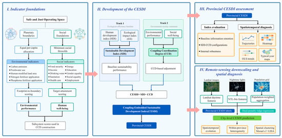
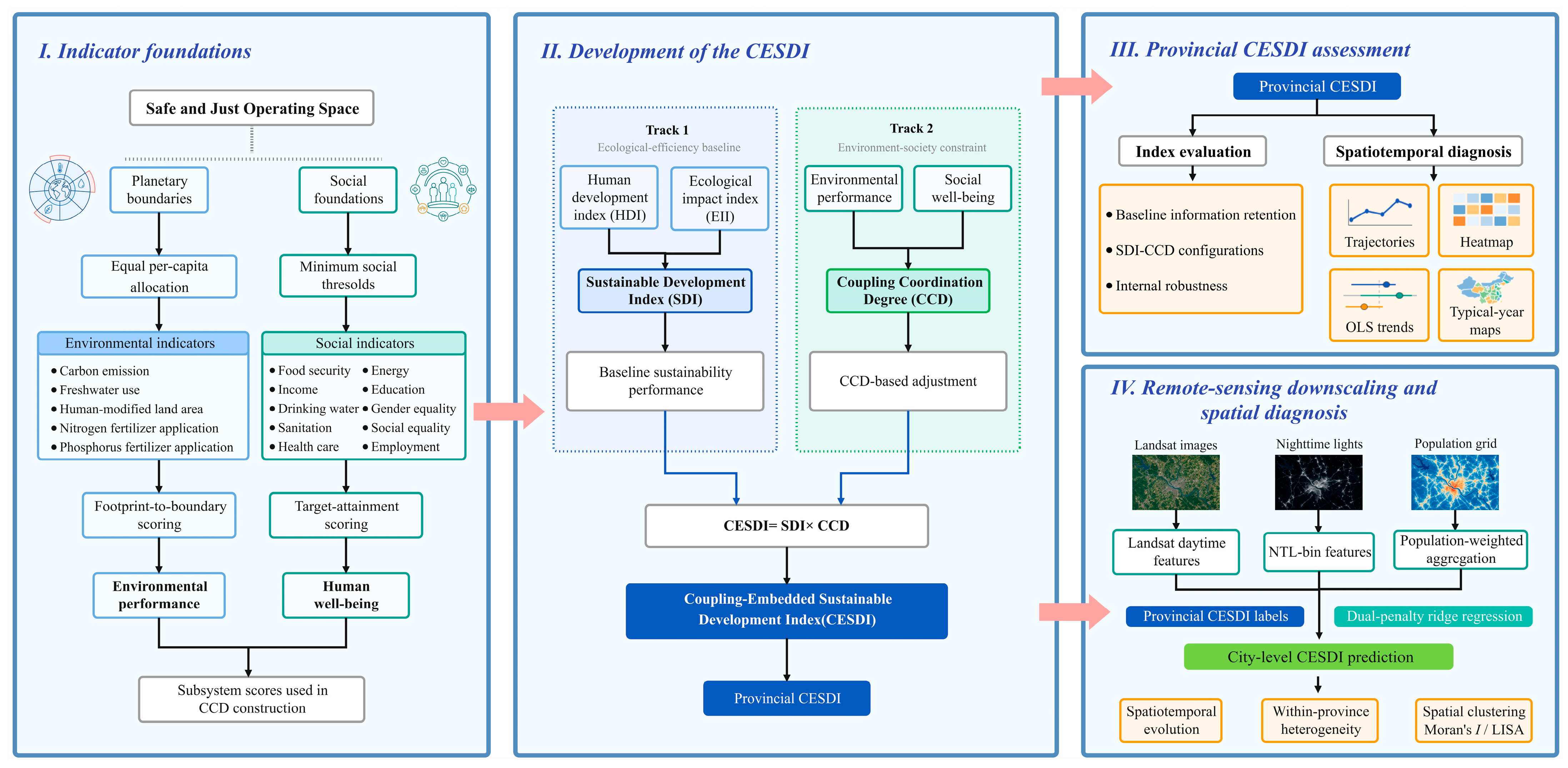
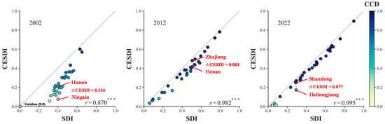
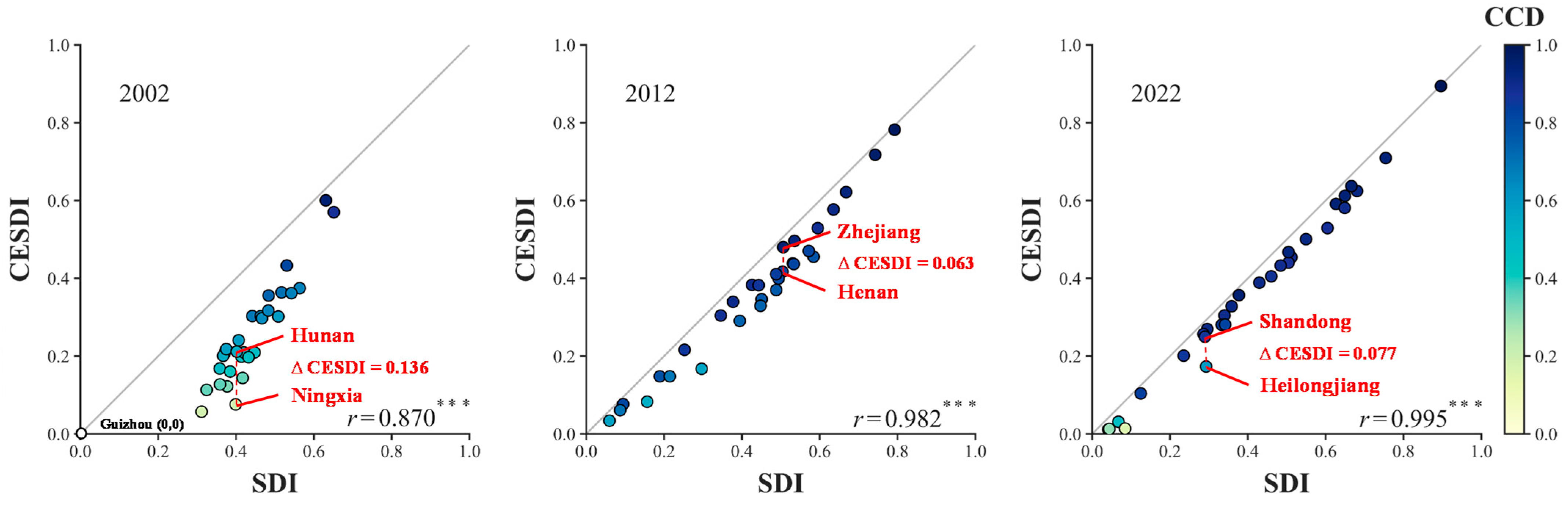
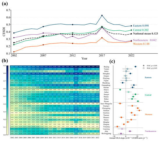
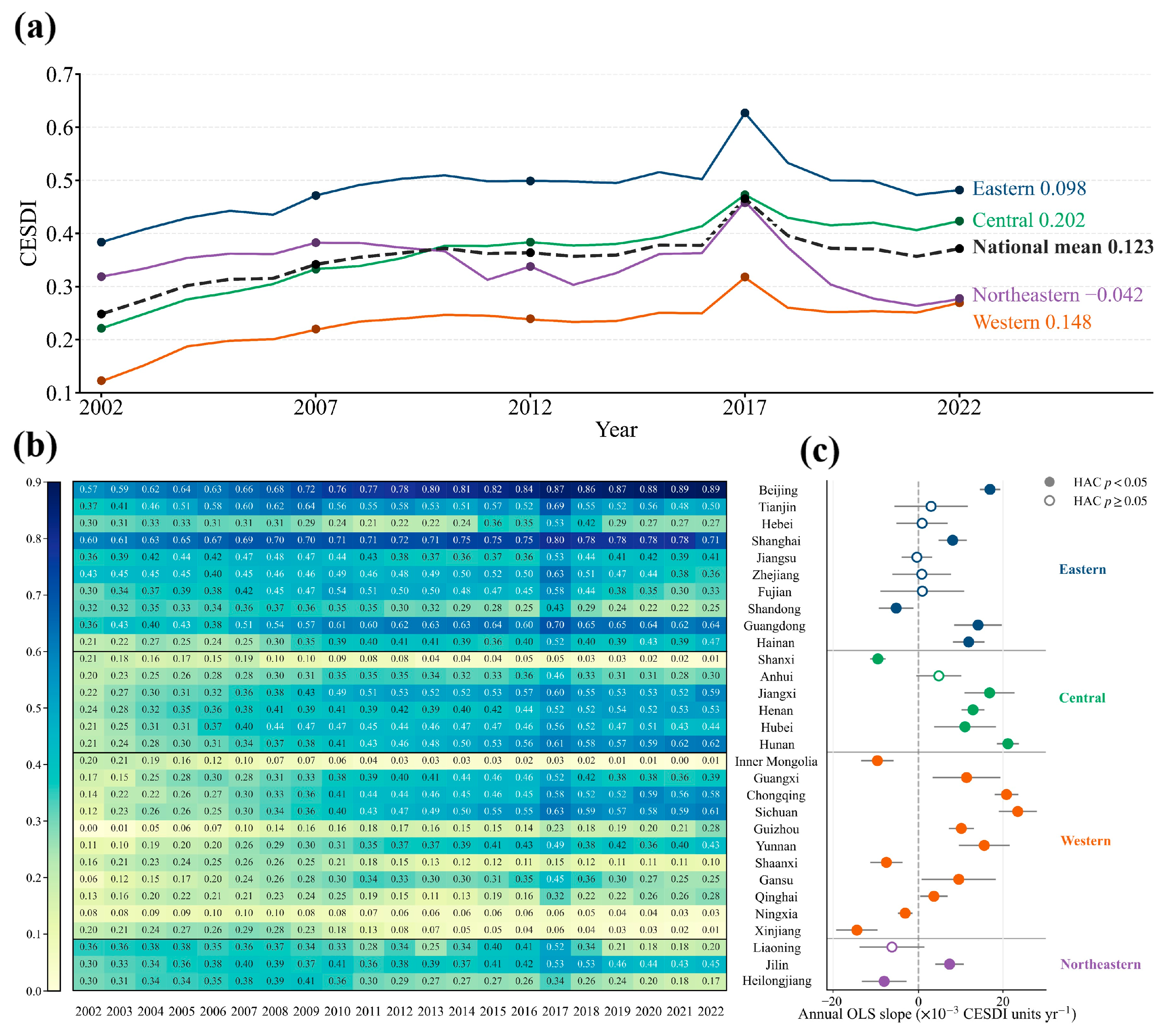
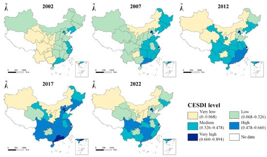
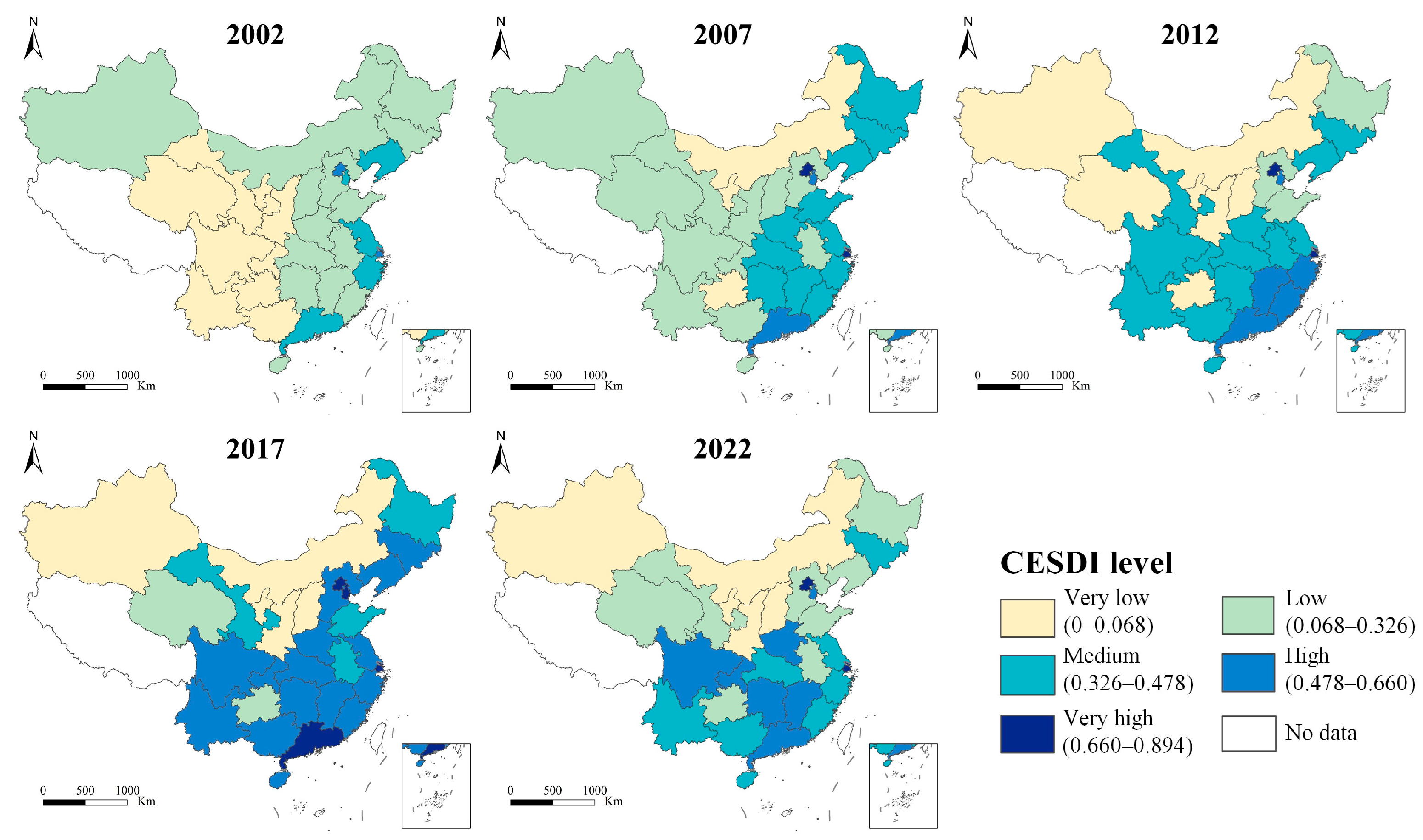
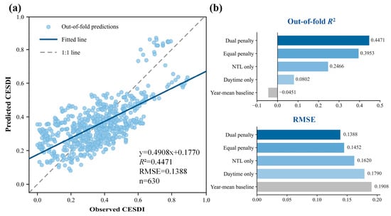
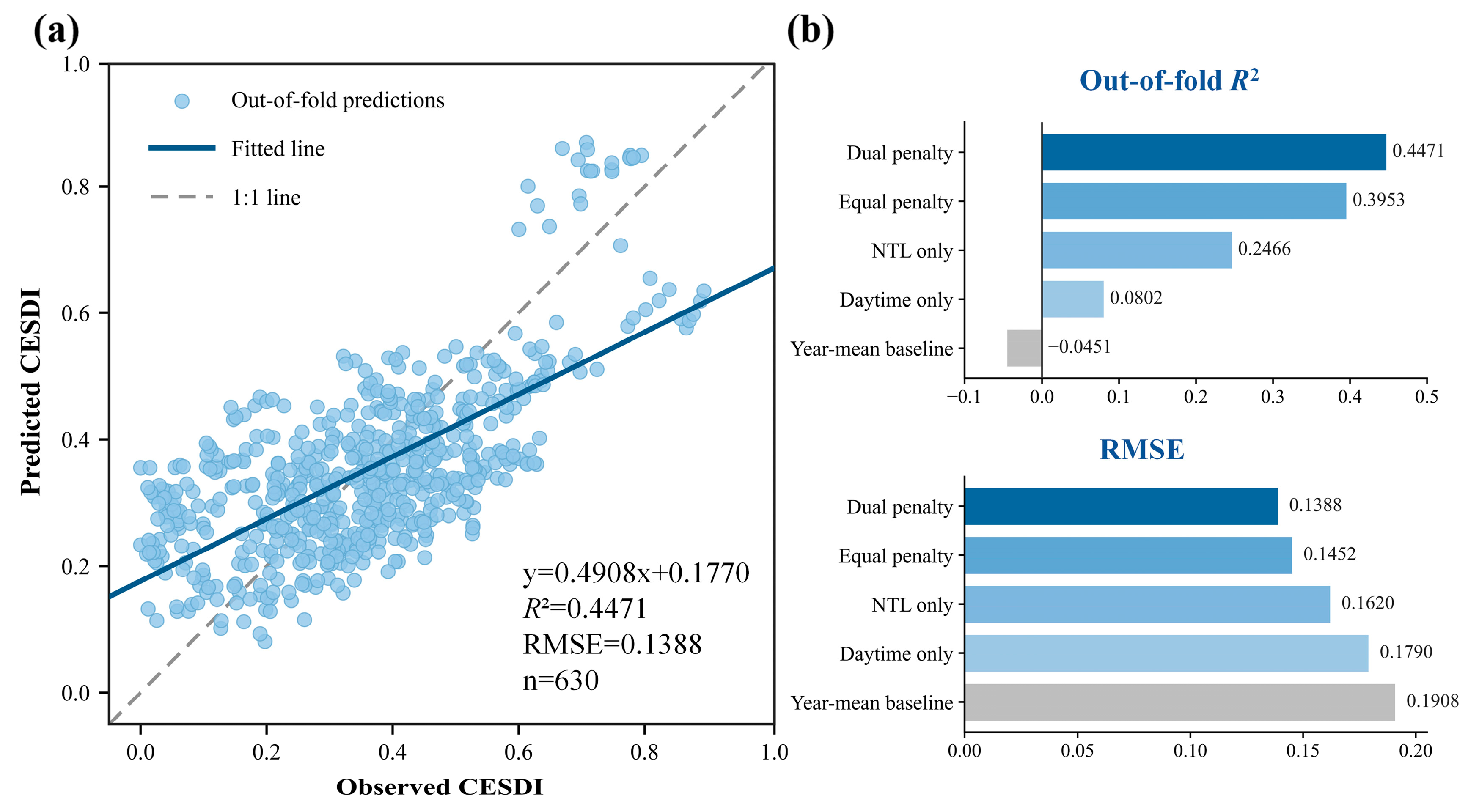
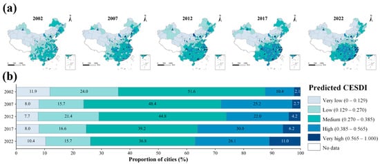
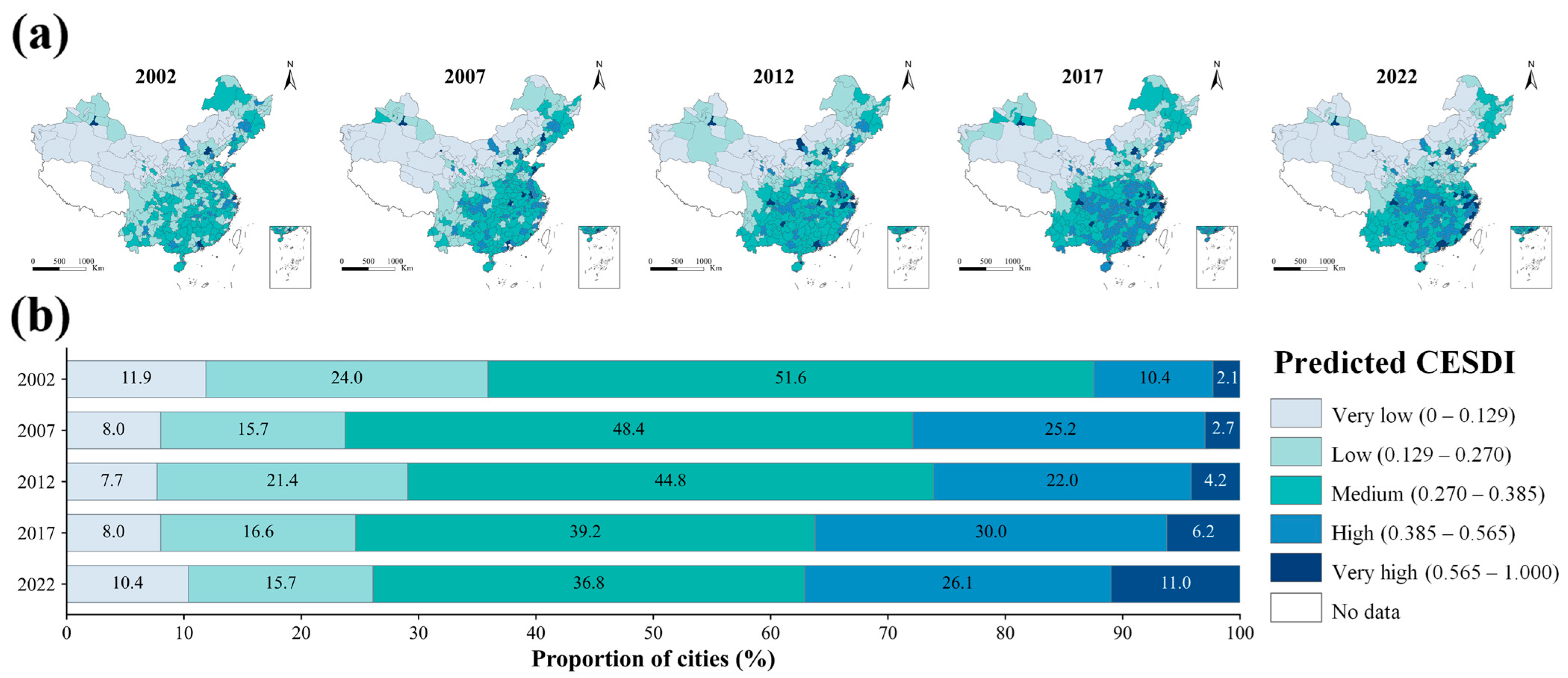
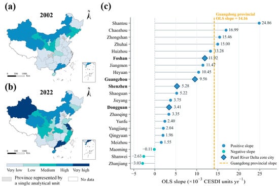
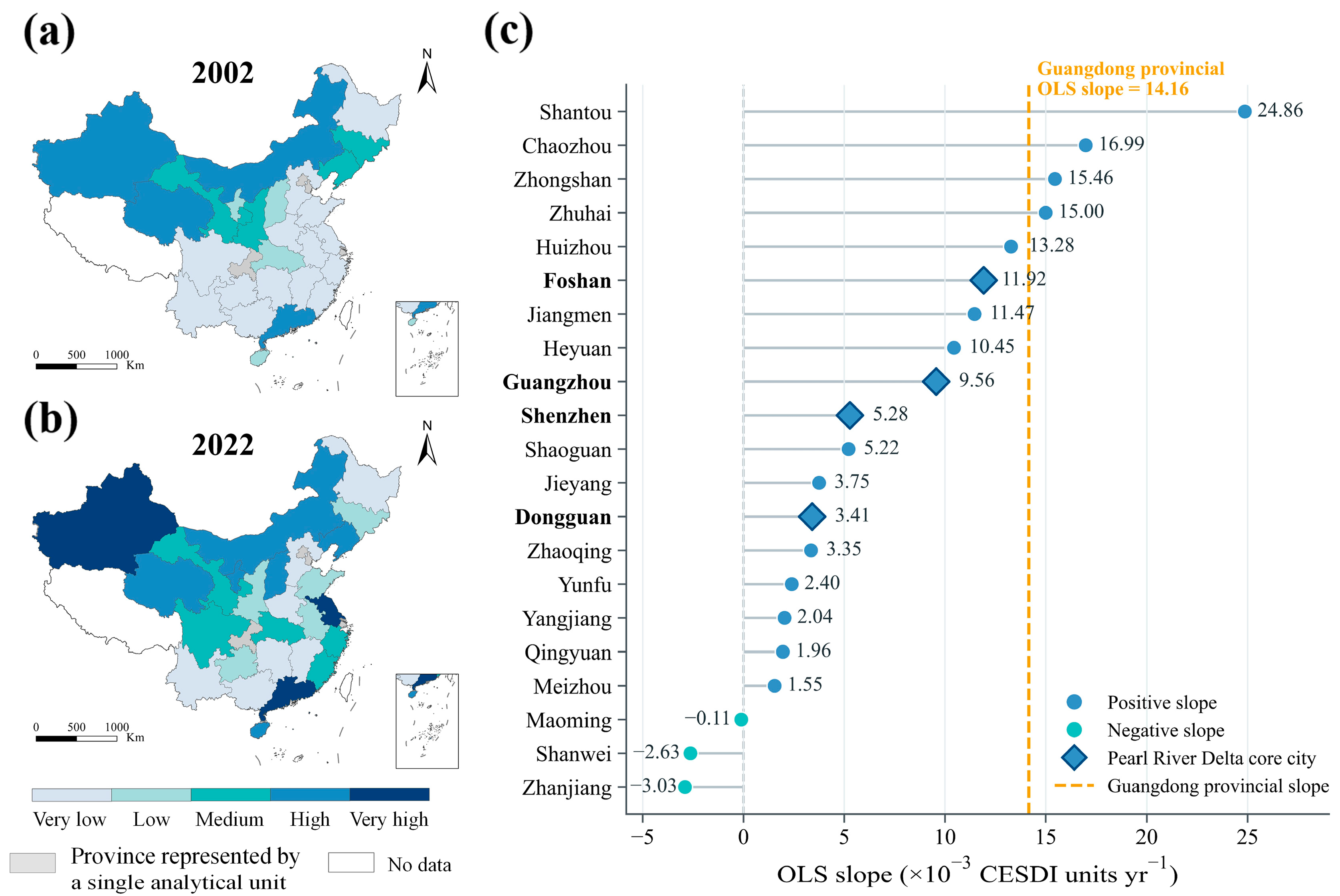
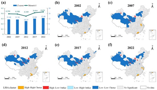
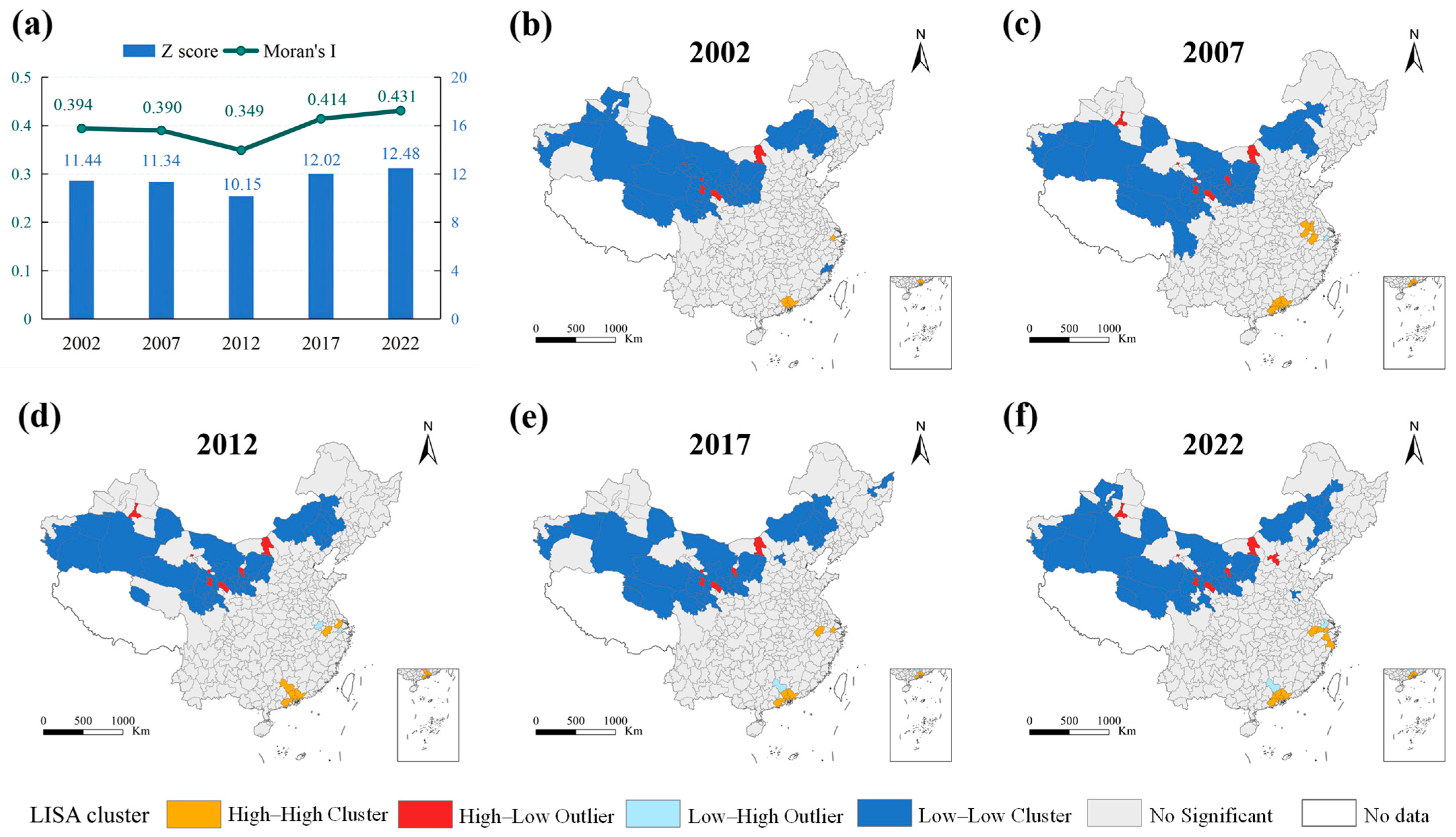

Disclaimer/Publisher’s Note: The statements, opinions and data contained in all publications are solely those of the individual author(s) and contributor(s) and not of MDPI and/or the editor(s). MDPI and/or the editor(s) disclaim responsibility for any injury to people or property resulting from any ideas, methods, instructions or products referred to in the content. |
© 2026 by the authors. Licensee MDPI, Basel, Switzerland. This article is an open access article distributed under the terms and conditions of the Creative Commons Attribution (CC BY) license.