


Highlights
What are the main findings?
- Zonal planetary waves 1 and wave 2 exert stage-separated forcing on polar vortex decay: wave 1 triggers the first warming peak, while amplified wave 2 dominates the second intense vortex disturbance.
- Wave–ozone coupling shows distinct wave-type and latitude selectivity: wave 1 at 60–70°S is associated with negative ozone anomalies over 0–50°S while wave 2 is associated with positive anomalies over 60–70°S during the 2024 Antarctic SSW.
What are the implications of the main findings?
- The stage-separated roles of wave 1 and wave 2 challenge the wave-1-dominated view of SSW forcing and highlight the importance of wave 2 in the Southern Hemisphere.
- Wave-type-selective ozone transport offers observational evidence for distinct dynamical pathways shaping Antarctic ozone variability during SSWs.
Abstract
Sudden Stratospheric Warmings (SSWs) are rare polar stratospheric extremes far less documented over Antarctica than the Arctic. A pair of successive midwinter Antarctic SSWs occurred in July–August 2024, featuring severe polar vortex distortion and sharp stratospheric temperature rises. Using MERRA-2/ERA5 reanalysis and MSR-2 total ozone column data, we diagnose wave 1 and wave 2 planetary wave forcing and associated ozone variations. Abnormally strong upward-propagating Southern Hemisphere tropospheric planetary waves drove the 2024 SSW. Wave 1 triggered the first July warming peak, while amplified wave 2 dominated the second intense vortex disruption in early August. These waves delivered westward momentum that weakened the polar night jet and destabilized the vortex. The ozone redistribution is consistent with an inferred enhancement of the Brewer–Dobson circulation (BDC) driven by the amplified wave activity, raising polar ozone levels and supplying extra stratospheric heat. Wave–ozone coupling shows clear selectivity: wave 1 is associated with negative total ozone column anomalies across 0–50°S (low-to-midlatitudes), whereas wave 2 is positively correlated with total ozone column anomalies over the 60–70°S polar collar region. Fading planetary wave activity after the warming peaks gradually restored the polar vortex and stratospheric thermal structure. This study provides key observational evidence for rare Antarctic SSWs and advances understanding of stratosphere–troposphere coupling and polar ozone dynamics under global warming.
1. Introduction
The stratosphere is a critical coupling layer connecting the troposphere and mesosphere, which exerts profound regulation on global large-scale atmospheric circulation and multi-timescale climate variability [1,2,3]. Sudden Stratospheric Warming (SSW) is the most intense dynamical extreme event in the polar stratosphere. It is defined as a rapid rise in polar temperature by several to tens of Kelvin within several days, accompanied by significant weakening, deformation or even breakdown of the stratospheric polar vortex (SPV). For major SSW events, the zonal-mean westerly wind at 10 hPa and 60° latitude may even reverse completely [4,5,6]. Following the standard WMO convention and the widely used definition from Andrews et al. [7], a major SSW is defined as a reversal of the zonal-mean zonal wind at 60°N/S and 10 hPa from westerly to easterly, whereas a minor warming (minor SSW) is a rapid stratospheric warming in which the zonal wind weakens significantly but does not reverse to easterly. SSW events involve complex dynamical, radiative and chemical feedbacks [8]. Their wave–mean flow interactions can reshape stratospheric circulation and propagate downward to modulate mid-latitude weather systems, cold surges, heatwaves and other extreme weather [9,10,11,12].
A remarkable hemispheric asymmetry exists in the climatology of SSW occurrence [13,14,15]. In the Northern Hemisphere (NH), SSWs occur frequently: minor warming events appear about once every 1–2 years, and major events with wind reversal recur every 2–4 years [5]. In sharp contrast, Antarctic SSWs are extremely rare. The core reasons include the nearly zonally symmetric Antarctic continent, weak meridional land–sea thermal contrast, and limited orographic forcing of planetary waves in the Southern Hemisphere midlatitudes [16,17,18]. Since the beginning of the satellite era in 1979, only one canonical major Antarctic SSW has been recorded, which occurred in September 2002 and featured full vortex splitting and zonal wind reversal [19,20]. This event was accompanied by significant total ozone anomalies and a split of the southern hemisphere ozone hole [21,22]. Two minor SSWs were separately documented in late winter 1988 and 2019, neither accompanied by complete zonal wind reversal [23,24]. Previous reanalysis studies have confirmed that the persistently strong polar night jet in austral winter suppresses the upward propagation of planetary waves and dynamically inhibits the formation of winter SSWs [25,26].
Planetary waves and the stratospheric polar vortex constitute the core dynamical system governing the onset and evolution of SSWs [27,28,29]. The winter polar vortex maintains a cold cyclonic circulation over the polar stratosphere, and its stability is predominantly controlled by vertical wave activity flux from the lower atmosphere, with the vortex-edge surf zone serving as the key region of wave dissipation and momentum deposition [30]. Tropospheric blocking highs over the Southern Ocean act as critical planetary wave sources that excite persistent upward wave propagation [31,32,33]. Existing investigations of the 2024 consecutive Antarctic SSWs indicate that sustained intense mid-high latitude tropospheric blocking triggered robust upward transport of wave 1 and wave 2 [34,35]. In addition, stratospheric preconditioning featured by negative meridional potential vorticity gradient and adjusted wave refractive index weakens vortex stability and facilitates planetary wave resonance amplification [36,37]. Nonlinear amplification of wave 2 jointly forced by tropospheric upward injection and in situ stratospheric excitation is widely accepted as a key driver of vortex splitting and severe attenuation during Southern Hemisphere SSWs [38,39].
Stratospheric ozone maintains tight dynamical-radiative-chemical coupling with SSWs [40,41,42,43]. Ozone effectively absorbs solar ultraviolet radiation and modulates stratospheric thermal and wind fields [3]. In turn, SSW-induced acceleration of the BDC enhances meridional ozone transport from subtropics toward the winter polar region [44]. Observations from historical Antarctic SSWs demonstrate strengthened residual circulation lifts polar total ozone column, suppresses heterogeneous chemical ozone loss on polar stratospheric clouds, and delays ozone hole formation [45].
Two successive winter SSWs hit Antarctica during July–August 2024, namely SW07 (6–13 July) and SW08 (21 July–5 August). Both events are classified as minor SSWs because the zonal-mean zonal wind at 60°S and 10 hPa weakened substantially (by approximately 23% between 13 July and 5 August, from ~74 to ~57 m s−1) but remained westerly throughout. This event set the record of the earliest winter SSW since satellite observations began and generated profound disturbances to polar vortex and ozone distribution [34,35]. Zi et al. [34] systematically diagnosed the troposphere-blocking-planetary wave cascade triggering SW07 and clarified that downward-propagating negative Southern Annular Mode signals originating from SW07 provided preconditioned circulation for SW08. Lim et al. [35] further pointed out that the 2024 SSW produced record-low Southern Annular Mode anomalies and induced extreme continental warming over Antarctica, representing an abnormal case of strong stratosphere–troposphere downward coupling rarely seen in austral winter. Nevertheless, prior research has not quantitatively identified the inherent correlations between multi-scale planetary wave variations and spatiotemporal ozone redistribution through correlation and spectral decomposition methods. Given the extreme scarcity of Antarctic winter SSWs and their far-reaching influences on polar ozone balance and mid-high latitude climate teleconnections, targeted dynamical diagnosis of the 2024 events carries essential theoretical and observational significance. This paper takes the two successive minor Antarctic SSWs in 2024 as research objects, systematically diagnoses the temporal, latitudinal and vertical evolution of wave 1 and wave 2, quantifies their modulating effects on polar vortex decay, and further discusses the dynamical coupling between planetary wave forcing and stratospheric ozone transport and redistribution throughout the warming lifecycle.
2. Materials and Methods
The study area focuses on the Southern Hemisphere during winter (June–August), with an emphasis on the Antarctic polar stratosphere, which is the core region where the 2024 sudden stratospheric warming (SSW) event occurred. This period corresponds to the polar night in the Antarctic region, during which the polar vortex is typically well-developed, and the stratospheric circulation is sensitive to planetary wave forcing, making it the key window for studying SSW events and their associated dynamical processes.
Four types of datasets are used in this study to ensure the comprehensiveness and reliability of the analysis: MERRA-2 (Modern-Era Retrospective analysis for Research and Applications, Version 2) reanalysis data, ERA5 reanalysis data, Aura MLS (Microwave Limb Sounder, National Aeronautics and Space Administration, USA) satellite observations, and the Multi-Sensor Reanalysis version 2 (MSR-2) total ozone product. MERRA-2 and ERA5 reanalysis data provide high-resolution atmospheric dynamical parameters (including temperature, zonal wind, meridional wind, and geopotential height) covering the troposphere and stratosphere, which are used to analyze planetary wave propagation and polar vortex variations. Aura MLS geopotential height data are used only for the wave amplitude diagnostics. Daily total ozone column (TOC) data were obtained from the MSR-2 dataset [45], produced by the Royal Netherlands Meteorological Institute (KNMI) and distributed through the Copernicus Climate Change Service (C3S). The MSR-2 dataset provides gap-free global TOC fields at a horizontal resolution of 0.5° × 0.5° spanning 1970 to the present, constructed by assimilating bias-corrected total ozone retrievals from 15 satellite instruments (including BUV, TOMS, SBUV series, GOME, SCIAMACHY, OMI, and GOME-2) together with ground-based Brewer and Dobson observations from the World Ozone and Ultraviolet Radiation Data Centre (WOUDC) into the TMDAM chemistry-transport model driven by ECMWF ERA-Interim reanalysis meteorology. Satellite observations are de-biased as a function of solar zenith angle, viewing zenith angle, temporal drift, and stratospheric temperature against the WOUDC ground-based reference, yielding a mean bias of less than 1% with respect to the de-biased satellite observations after 1979. The MSR-2 data were used here to provide the long-term climatological context (2005–2024) against which the 2024 SH SSW ozone anomalies were evaluated. For MERRA-2 and ERA5, the climatological mean is computed over 1979–2024 (46 years), consistent with the MERRA-2 data record starting from January 1979; for the MSR-2 total ozone column, the climatological mean is computed over 2005–2024. All datasets are processed to ensure consistency and applicability for the research objectives.
The data are obtained from the following archives: MERRA-2, NASA Global Modeling and Assimilation Office (GMAO)/GES DISC, https://gmao.gsfc.nasa.gov/reanalysis/MERRA-2/, accessed on 10 July 2026; ERA5, Copernicus Climate Data Store (CDS), https://cds.climate.copernicus.eu/, accessed on 20 June 2026; Aura MLS, NASA JPL Microwave Limb Sounder, https://mls.jpl.nasa.gov/, accessed on 4 August 2026; MSR-2 total ozone column, KNMI TEMIS, https://www.temis.nl/protocols/O3global.php (https://doi.org/10.21944/temis-ozone-msr2), accessed 15 July 2026.
Table 1 summarizes the four datasets used in this study, giving for each product the variables extracted, the horizontal and vertical resolutions, and the temporal resolution. MERRA-2 and ERA5 are the primary gridded reanalyses, Aura MLS provides the geopotential height wave amplitude used for the vertical structure analysis, and MSR-2 supplies the daily total ozone column analysys.
Table 1.
Datasets used in this study.
Table 2 defines the event labels used throughout the text. SSW88, SSW02 and SSW19 denote the three historical Antarctic SSWs used for comparison, SSW24 denotes the 2024 season as a whole, and SW07 and SW08 denote its two consecutive warming pulses.
Table 2.
Correspondence between the event labels used in this study and the dates of each event.
The geopotential height data from the Aura Microwave Limb Sounder (MLS) are interpolated onto a regular longitudinal grid of 360 points (0–359°) for each pressure level and day. The MLS retrievals are valid between approximately 100 hPa and 0.1 hPa (roughly 16–64 km geometric height), and pressure levels are converted to geometric height using the U.S. Standard Atmosphere. Planetary waves at zonal wavenumbers 1 (wave 1) and 2 (wave 2) are then extracted via a discrete Fourier transform (DFT) along the longitudinal dimension, which decomposes the geopotential height field into wavenumber space:
where Z(λj, ϕ, p, t) denotes the gridded geopotential height as a function of longitude λj, latitude ϕ, pressure level p, and time t; is the complex Fourier coefficient at zonal wavenumber k; and the normalization factor 1/N ensures that the zero-wavenumber component directly equals the zonal-mean value. For real-valued geopotential height fields, the coefficients satisfy conjugate symmetry . The wave amplitude at wavenumber k is defined as twice the magnitude of the single-sided coefficient: giving the actual peak-to-mean amplitude in geopotential height (units: meters).
To reconstruct the spatial structure of wave 1 and wave 2, a spectral filter H1,2(k) that equals unity for k = ±1 or k = ±2 and zero otherwise is applied, and the filtered field is transformed back to longitude space via the inverse DFT:
where Z1 and Z2 denote the reconstructed wave 1 and wave 2 spatial components, respectively. Both positive and negative wavenumber components are retained in the reconstruction to ensure the resulting field remains real-valued. The resulting Z1,2(λj, ϕ, p, t) represents the day-to-day spatial pattern of planetary wave 1 and wave 2 at each latitude and pressure level.
3. Results
3.1. Zonal Mean Temperature and Zonal Wind
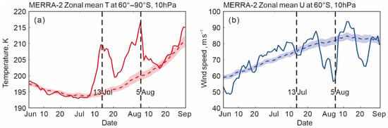
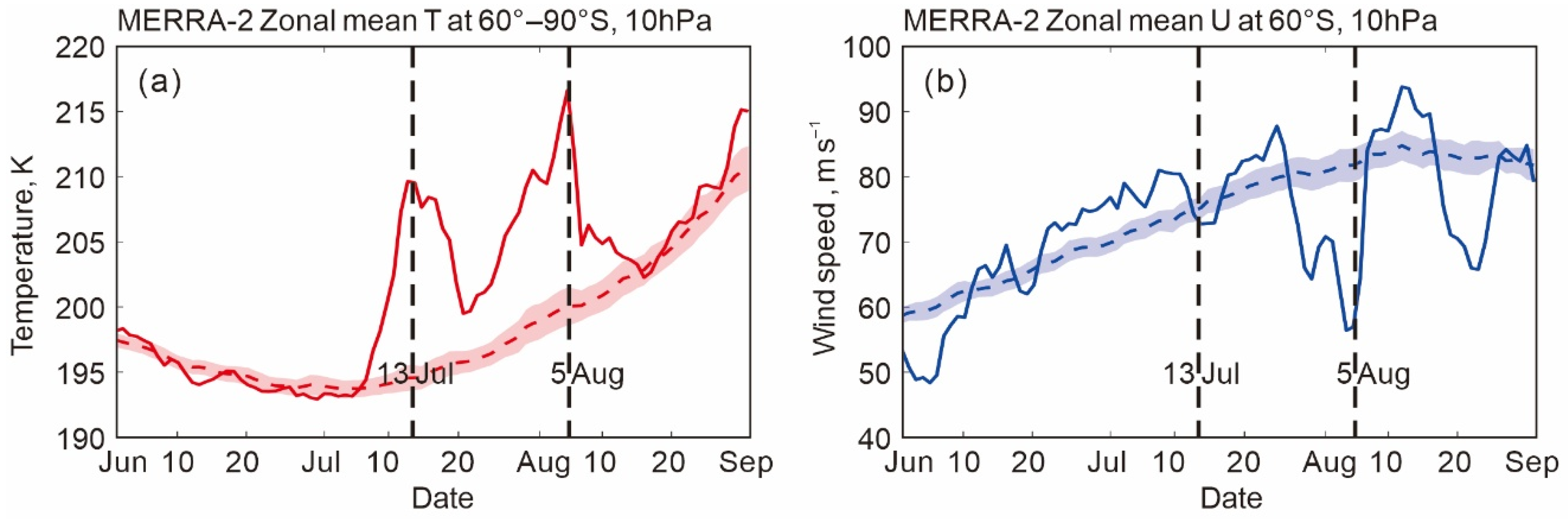
The time series of daily zonal-mean parameters at 10 hPa over the Antarctic region, derived from MERRA-2 reanalysis data, is shown in Figure 1, which is divided into two panels: panel (a) presents the zonal-mean temperature (K) averaged over 60–90°S, while panel (b) displays the zonal-mean zonal wind speed (m s−1) at 60°S. The dashed line in both panels represents the climatological mean of the corresponding parameters over the period 1979–2024, and the shaded area around the dashed line denotes the 95% confidence interval. The 95% confidence interval (shaded band) of the daily climatological mean was constructed using Student’s t-distribution. For each calendar day d, the climatological mean was computed as , where N = 46 is the number of years (1979–2024). The sample standard deviation was calculated as , and the standard error of the mean was obtained as . The 95% confidence interval was then given by , where tN−1,0.025 is the two-sided 0.025 critical value of Student’s t-distribution with N − 1 degrees of freedom (t45,0.025 ≈ 2.014). Note that this interval represents the sampling uncertainty of the climatological mean rather than the interannual variability of the raw daily values, which is why the shaded band is relatively narrow (see Supplement S2 for details).
Figure 1.
Time series of daily 10 hPa MERRA-2 reanalysis zonal mean (a) temperature at 60–90°S and (b) zonal wind at 60°S, 10 hPa, during June–September 2024. The vertical dashed lines mark 13 July and 5 August 2024, the two dates when the temperature reached its peak values. The dashed line denotes the climatological mean over the period 1979–2024, with the shaded area representing the 95% confidence interval, both calculated as described in the text above.
Two vertical dashed lines are added to mark 13 July and 5 August 2024, the two key dates when the stratospheric temperature reached its peak values during the 2024 Antarctic sudden stratospheric warming (SSW) event.
Clear temporal variations of the mean zonal wind can be observed throughout the SSW event: before the onset of the SSW (early July 2024), the mean zonal wind at 60°S and 10 hPa maintains a relatively high value of approximately 70 m s−1, indicating a well–developed and stable Antarctic polar vortex. As the SSW event progresses, the zonal wind shows a continuous and dramatic downward trend, with the most significant deceleration occurring during the peak period of the SSW. By the late stage of the SSW (early August 2024), the mean zonal wind decreases to around 57 m s−1 on 5 August, a reduction of approximately 23% from ~74 m s−1 on 13 July to ~57 m s−1 on 5 August. Following this minimum, the zonal wind recovers progressively. This sharp decline in zonal wind is closely associated with the upward propagation of anomalous planetary waves during the 2024 SSW, which deposit westward momentum and weaken the polar night jet, further leading to the weakening and distortion of the Antarctic polar vortex.
Obvious variations of the parameters can be observed in the time series: in Figure 1a, the zonal mean temperature at 60–90°S and 10 hPa shows a significant upward trend from early July 2024, rising from around 194 K (7 July) to the first peak of approximately 210 K on 13 July, followed by a slight decline and then another upward trend to the second peak of about 217 K on 5 August. Throughout the entire observation period, the daily temperature values are consistently higher than the climatological mean and mostly outside the 95% confidence interval, indicating the anomalous nature of the 2024 SSW-related warming (see Figure S1 in Supplement S3 for details). In panel (b), the zonal wind at 60°S and 10 hPa strengthens from approximately 50 m s−1 in early June to a local maximum of approximately 88 m s−1 in late July, before decreasing sharply to approximately 57 m s−1 on 5 August. Following this minimum, the wind rebounds rapidly to approximately 93 m s−1 in mid-August, indicating a quick recovery of the polar vortex that reflects the strengthening of planetary wave activities during the SSW event.
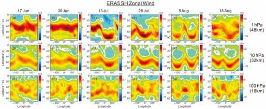
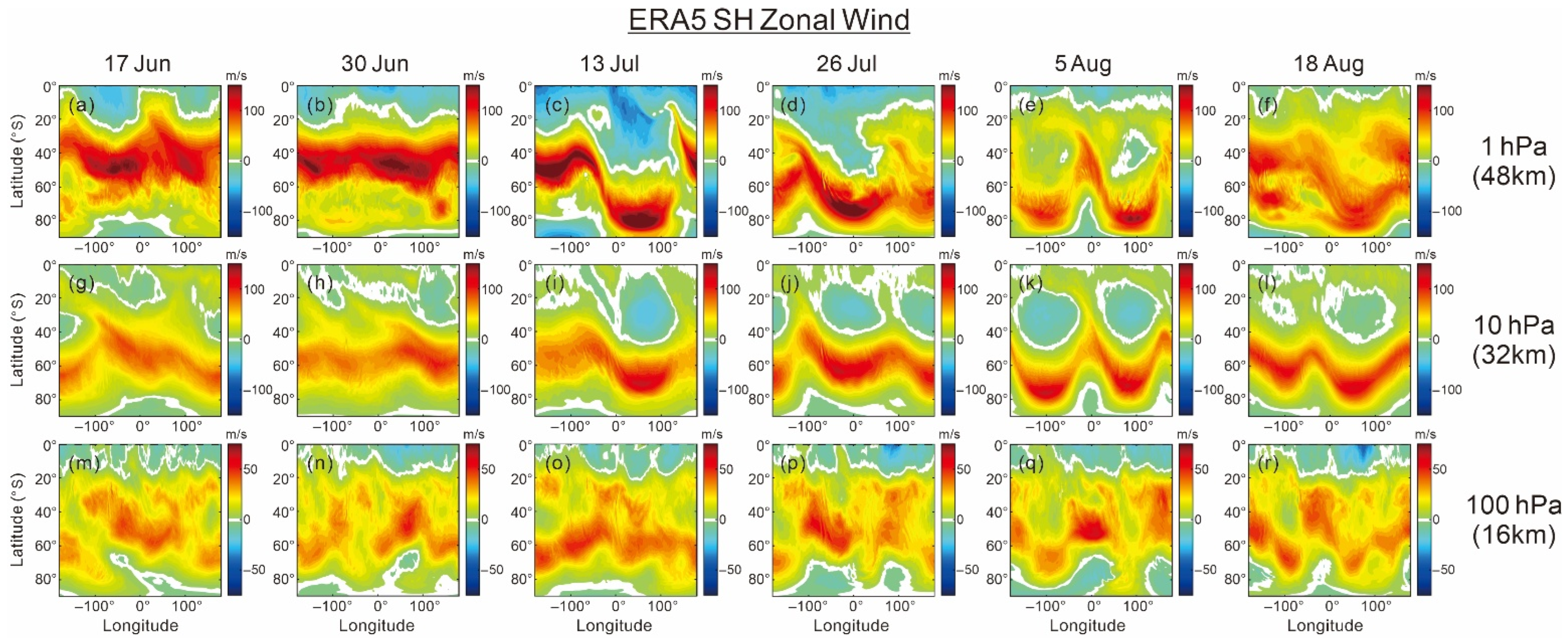
Figure 2 displays the Southern Hemisphere zonal wind fields from ERA5 reanalysis data across three stratospheric levels during June to August 2024, covering the period before and during the Antarctic sudden stratospheric warming (SSW). At the pre-SSW stage in early June, a strong westerly polar night jet dominated southern latitudes 40–60°S. The maximum wind speed reached 120–150 m s−1 at the 48 km stratopause and 80–100 m s−1 at the 32 km middle stratosphere, sustaining a stable polar vortex. As the SSW developed from mid-July, the westerly jet weakened at mid-latitudes and contracted poleward. By 5 August, the westerly circulation developed two lobes at both 1 and 10 hPa, one centered near 65–80°S, 80–120°W and the other near 65–80°S, 80–120°E, indicating elongation and distortion of the vortex rather than a complete split (Figures S4 and S5).
Figure 2.
The zonal wind field over SH (0–90°S) on selected dates between 1 June and 31 August from the ERA5 reanalysis: (a–f) stratopause (48 km); (g–l) middle stratosphere (32 km); (m–r) lower stratosphere (16 km) levels before and during the SSW event.
The vertical discrepancy of wind anomalies reflects the typical dynamical characteristics of Antarctic SSW events. Disturbances in the zonal flow first emerged in the upper stratosphere and then gradually descended to lower levels, with anomaly intensity decreasing evidently with decreasing altitude. From late July to August, the stratospheric wind field experienced a full cycle of jet weakening and gradual recovery. The overall spatiotemporal variation of zonal winds clearly depicts the entire evolution of polar vortex disturbance and stratospheric circulation adjustment throughout the 2024 Antarctic SSW event.
3.2. Planetary Wave 1 and 2
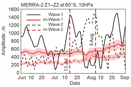
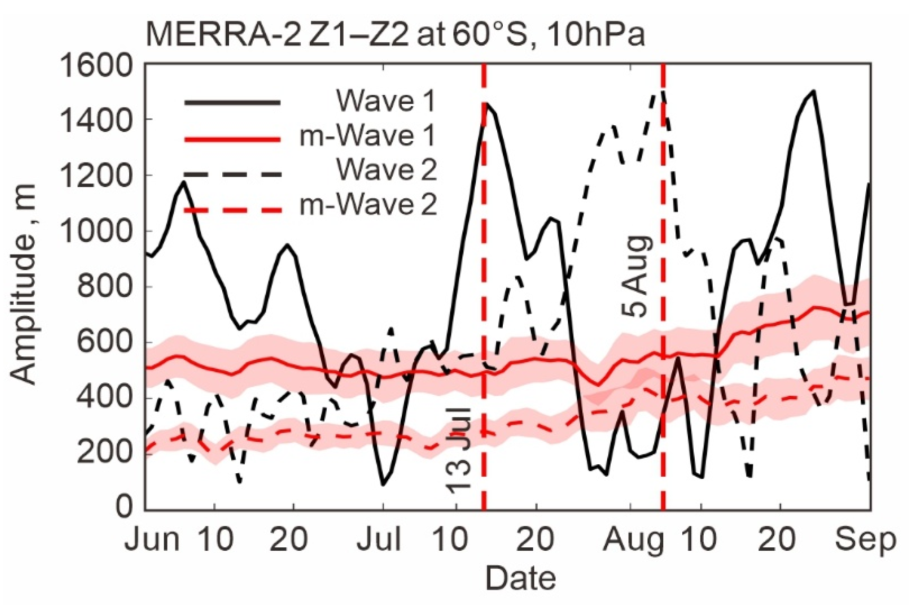
Figure 3 presents the time series of zonal wave 1 and wave 2 amplitudes in geopotential height at 60°S and 10 hPa during June–August 2024, derived from MERRA-2 reanalysis time series data. This figure focuses on the temporal evolution of planetary wave amplitudes, which are key indicators of planetary wave activity and play a crucial role in triggering and maintaining the 2024 Antarctic Sudden Stratospheric Warming (SSW) event. Two vertical dashed lines are included in the figure, representing 13 July and 5 August 2024 respectively, which correspond to the two temperature peak dates of the 2024 SSW event. Additionally, the red solid line and red dashed line in the figure denote the climatological mean of the wave 1 and wave 2 amplitudes over the period 1979–2024, while the shaded area represents the 95% confidence interval of the climatological mean.
Figure 3.
Daily amplitudes of planetary wave 1 (solid lines) and wave 2 (dashed lines) in geopotential height at 60°S and 10 hPa during June–August 2024 from the MERRA-2 reanalysis. Red lines show the corresponding climatological mean (1979–2024) for each calendar day, with the shaded area representing the 95% confidence interval of the climatological mean. The vertical dashed lines mark 13 July and 5 August.
Distinct variations in wave 1 and wave 2 amplitudes can be observed throughout the study period (June–August 2024). During early June, wave 1 amplitude is already at a moderately high level (923 m on 1 June), while wave 2 remains relatively weak (268 m on 1 June). Following a transient peak in mid-June (1175 m on 6 June), wave 1 declines through early July before rising sharply to 1454 m on 14 July. In contrast, wave 2 stays moderate through the first half of July and shows a distinct secondary enhancement in late July, before intensifying markedly in early August and surging to its peak near 5 August. These peak values are significantly higher than the climatological mean and well outside the 95% confidence interval, indicating anomalous enhancement of planetary wave activity during the SSW peak periods. After mid-August, new peaks emerged for both waves: wave 1 reached approximately 1500 m around 23 August, and wave 2 sustained values of 100–1000 m through 15–20 August, before both amplitudes decreased toward late August. This variation pattern of planetary wave amplitudes is closely associated with the evolution of the 2024 SSW event, as the enhanced upward propagation of wave 1 and wave 2 delivers westward momentum to the stratosphere, contributing to the polar vortex weakening and stratospheric warming.
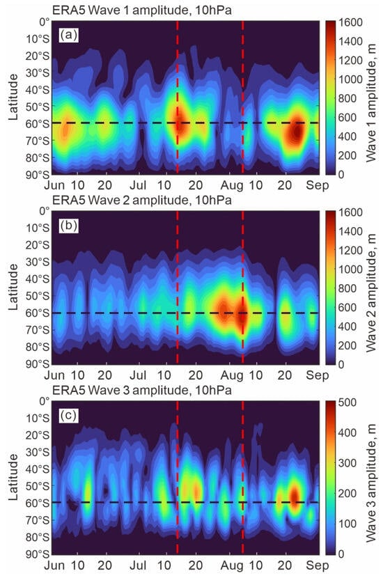
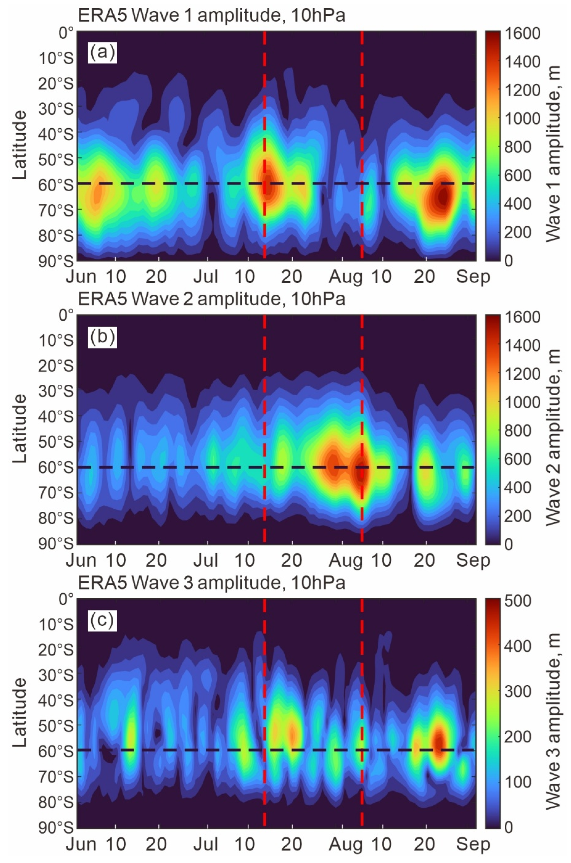
Complementing the temporal analysis at 60°S, the latitude–time cross-sections of planetary wave amplitudes (Figure 4) from ERA5 data further contextualize the spatial and temporal evolution of wave activity across the Southern Hemisphere stratosphere at 10 hPa during June–September 2024.
Figure 4.
Latitude—time cross-section of the amplitudes of planetary (a) wave 1, (b) wave 2, (c) wave 3 at 10 hPa in Southern Hemisphere (SH) by ERA5 data. Dashed horizontal lines mark the mean vortex edge latitude of 60°S.
Consistent with the MERRA-2 time series results, the cross sections confirm that the strongest wave forcing during the SSW event was concentrated in mid-to-high latitudes (50–80°S), near the climatological polar vortex edge at 60°S (see Figure 4). For wave 1 (Figure 4a), a single prominent amplitude maximum is observed on 14 July, with peak values exceeding 1400 m near 60–70°S. This aligns with the first warming peak of the 2024 SSW and indicates that wave 1 was the dominant wave contribution to the initial vortex weakening. Wave 2 activity (Figure 4b) shows a pronounced enhancement centered on 5 August, with peak amplitudes reaching approximately 1500 m. This corresponds to the second warming phase of the SSW, indicating that wave 2 forcing was closely associated with the amplification of vortex disruption. In contrast, wave 3 (Figure 4c) amplitude remains much weaker throughout the period with small enhancement during the SSW event. This indicates that wave 3 played a negligible role in the 2024 Antarctic SSW, consistent with the established understanding that wavenumbers 1 and 2 are the primary planetary wave drivers of Southern Hemisphere stratospheric sudden warmings.
Across all three waves, the vertical dashed lines highlight the key transition periods of the SSW, demonstrating that the anomalous wave activity was confined to the mid-to-high latitudes where the polar vortex is most vulnerable to wave forcing. Together, the time series and latitude–time cross-section analyses confirm that the sequential, climatologically anomalous enhancement of wave 1 and wave 2 activity were closely associated with the two-stage weakening of the Antarctic polar vortex and the associated stratospheric warming in 2024.
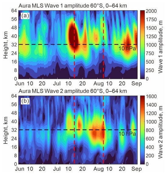
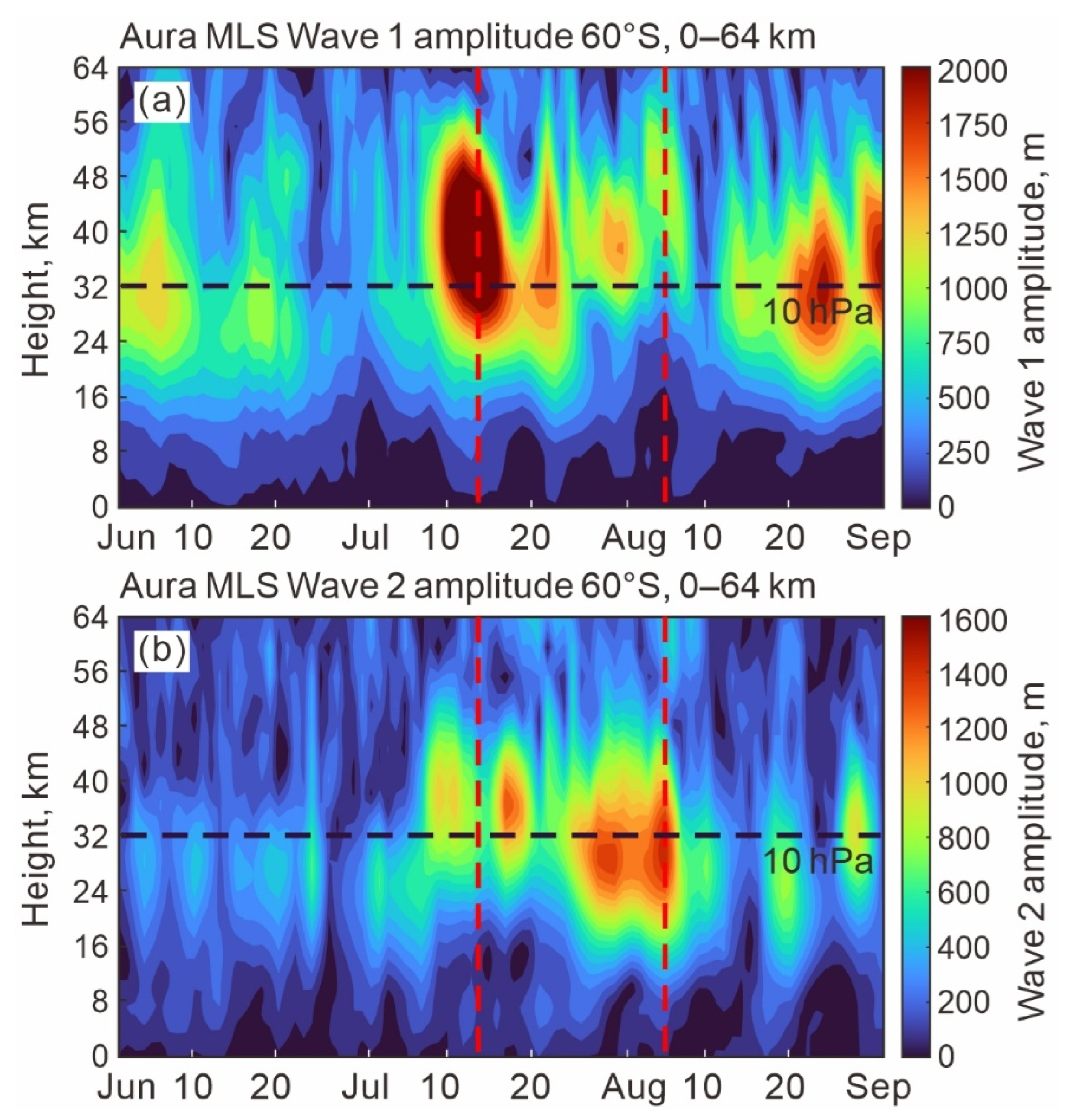
Figure 5 further extends the analysis by presenting height–time cross-sections of wave 1 and wave 2 amplitudes at 60°S from 0 to 64 km, based on Aura MLS observations, revealing the vertical structure of wave activity during the same period.
Figure 5.
The amplitudes (a) Z1 and (b) Z2 at 60°S in pressure—time section for June–August 2024 by Aura MLS data. Dashed horizontal lines mark the stratosphere level at 10 hPa.
For wave 1 (Figure 5a), a vertically coherent maximum is observed in mid-July, spanning approximately 20–50 km with peak amplitudes exceeding 1750 m near 40 km (above the 10 hPa level), indicating strong upward propagation into the upper stratosphere during the early SSW phase. In late July to August, wave 1 amplitudes weaken considerably at 20–40 km and do not sustain significant forcing through the second warming peak. Wave 2 (Figure 5b) exhibits a delayed but vertically extensive enhancement peaking in late July to early August, spanning approximately 20–45 km with maximum amplitudes of approximately 1400 m in the 25–35 km layer (centered on 10 hPa), reflecting middle-stratospheric forcing during the vortex disruption phase.
Collectively, the multi-dataset analysis of temporal, latitudinal, and vertical variations in wave amplitudes demonstrates that sequential, climatologically anomalous enhancements of wave 1 and wave 2 activity were closely associated with the two-stage evolution of the 2024 Antarctic SSW, with wave 1 dominating the early phase and wave 2 dominating during the peak warming period.
Beyond the amplitude diagnostics presented above, wavenumber-resolved Eliassen–Palm (EP) fluxes and their divergence for wave 1 and wave 2 were computed from daily ERA5 fields in order to examine the upward propagation and momentum deposition associated with the two warming phases. These flux-level diagnostics support the wave forcing interpretation drawn from the amplitude evolution and are provided in the Supplementary Material (Figures S3 and S6).
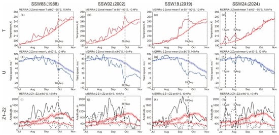
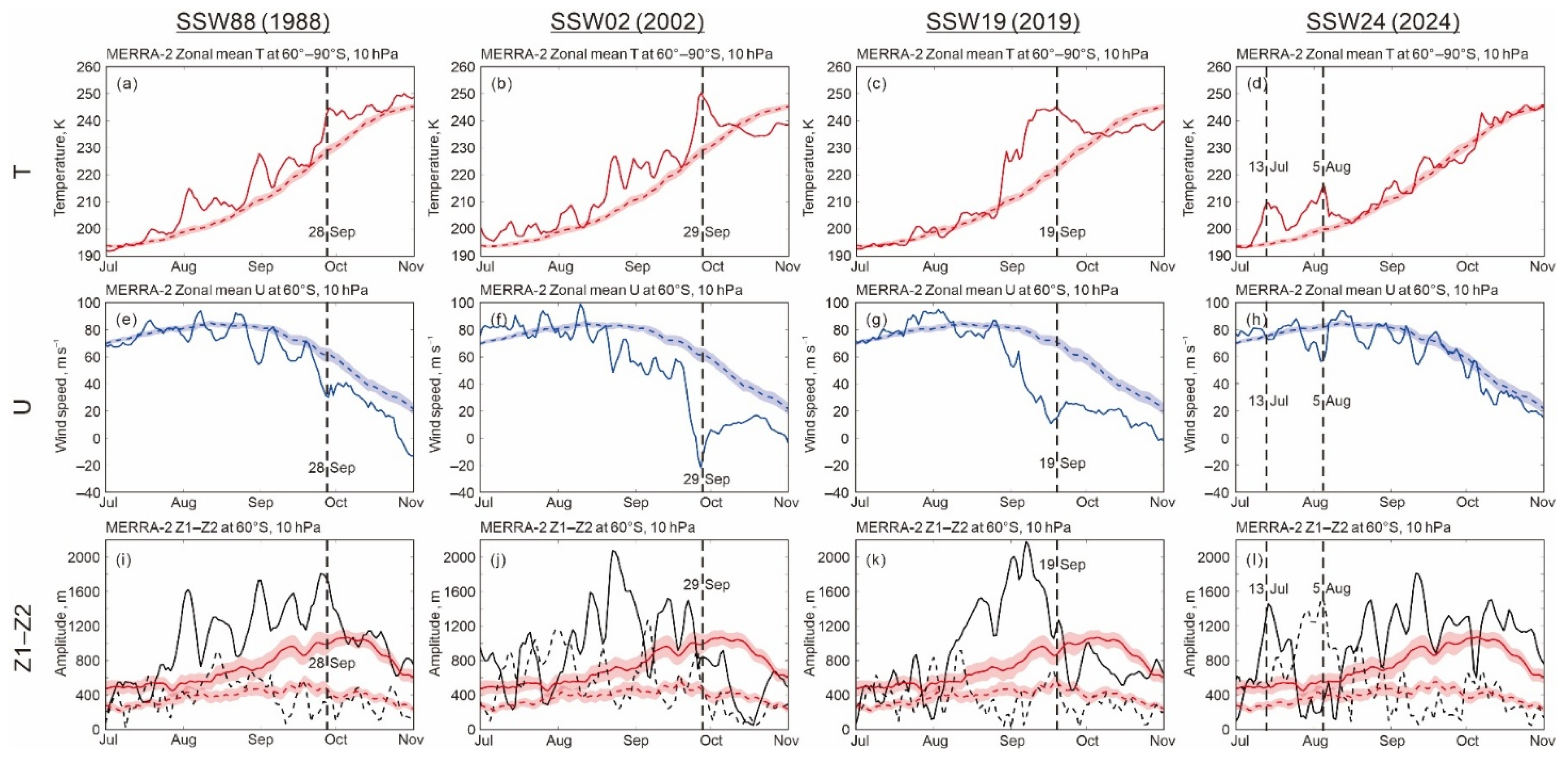
To contextualize the 2024 Antarctic stratospheric warming within the broader record of Southern Hemisphere stratospheric variability, a comparative analysis of three historical Southern Hemisphere SSW events, namely SSW88 (1988), SSW02 (2002), and SSW19 (2019), together with SSW24 (2024), are shown in Figure 6. Panels (a–d) show zonal-mean polar temperatures (60–90°S), (e–h) zonal winds at 60°S, and (i–l) planetary wave 1 (solid) and wave 2 (dashed) amplitudes at 60°S, all at 10 hPa and spanning 1 July–31 October. Vertical dashed lines mark the date of maximum temperature of each event, while the red/blue dashed line and shaded red/blue area denote the 1979–2024 climatological mean and 95% confidence interval, respectively. Across all four events, clear common patterns emerge: early winter conditions are characterized by near-climatological polar temperatures (~190–200 K on 1 July) and a strong, stable polar night jet (~60–80 m s−1 on 1 July), while the SSW events display distinct warming signatures, with SSW88 peaking at T ≈ 245 K on 28 September (u ≈ 30 m s−1), SSW02 at T ≈ 250 K on 27 September (u ≈ −22 m s−1, wind reversal), SSW19 at T ≈ 245 K on 19 September (u ≈ 14 m s−1), and SSW24 showing two consecutive minor peaks at T ≈ 210 K on 13 July and T ≈ 217 K on 5 August (u ≈ 57 m s−1, no wind reversal). Each event is preceded by a pronounced enhancement of planetary wave activity, indicating that enhanced upward wave propagation is closely associated with vortex disruption and stratospheric warming.
Figure 6.
Comparison of four Southern Hemisphere SSW events: SSW88 (1988), SSW02 (2002), SSW19 (2019), and SSW24 (2024). (a–d) Zonal mean temperature averaged over 60–90°S; (e–h) zonal wind at 60°S; (i–l) planetary wave 1 (solid) and wave 2 (dashed) amplitudes at 60°S. All variables are at 10 hPa and cover the period from 1 July to 31 October. The vertical black dashed lines indicate the dates with the highest temperature. The red/blue dashed line denotes the 1979–2024 climatological mean, with the shaded area representing the 95% confidence interval.
Despite these shared characteristics, the events exhibit key differences in intensity, timing, and wave forcing dynamics. SSW88 represents a minor event, with temperatures rising only ~15 K above the climatological mean (a peak of 244.6 K on 28 September against the 1979–2024 climatological mean of 229.3 K) and the zonal wind weakening but remaining positive, dominated almost entirely by wave 1 forcing with minimal wave 2 contribution. SSW02 is a major SSW, featuring a sharp temperature rise (~22 K above climatology), a complete reversal of the zonal wind, and a secondary enhancement of wave 2 activity that amplifies vortex disruption. SSW19 is a minor SSW, with temperatures peaking ~23 K above climatology, a dramatic collapse of the polar night jet, and a particularly prominent, early wave 1 peak that is associated with strong vortex weakening.
SSW24 is fundamentally different from the other three SSWs. First, it occurred earliest, with two consecutive warming pulses occurring in midwinter (13 July and 5 August) rather than in early spring, when the climatological background temperature is still relatively low. Second, the polar night jet remains strong (minimum 57 m s−1 on 5 August) with no wind reversal, confirming its minor SSW classification. Third, SSW24 is the only event with two distinct warming pulses within a single season, driven by a sequential switch from wave 1 (peak ~1454 m on 14 July) to wave 2 (peak ~1511 m on 5 August). These variations highlight that while planetary wave activity is the common driver, differences in the timing, magnitude, and relative contributions of wave 1 and wave 2 lead to distinct SSW intensities and vortex responses in the Southern Hemisphere.
3.3. Total Ozone Column
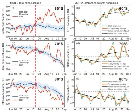
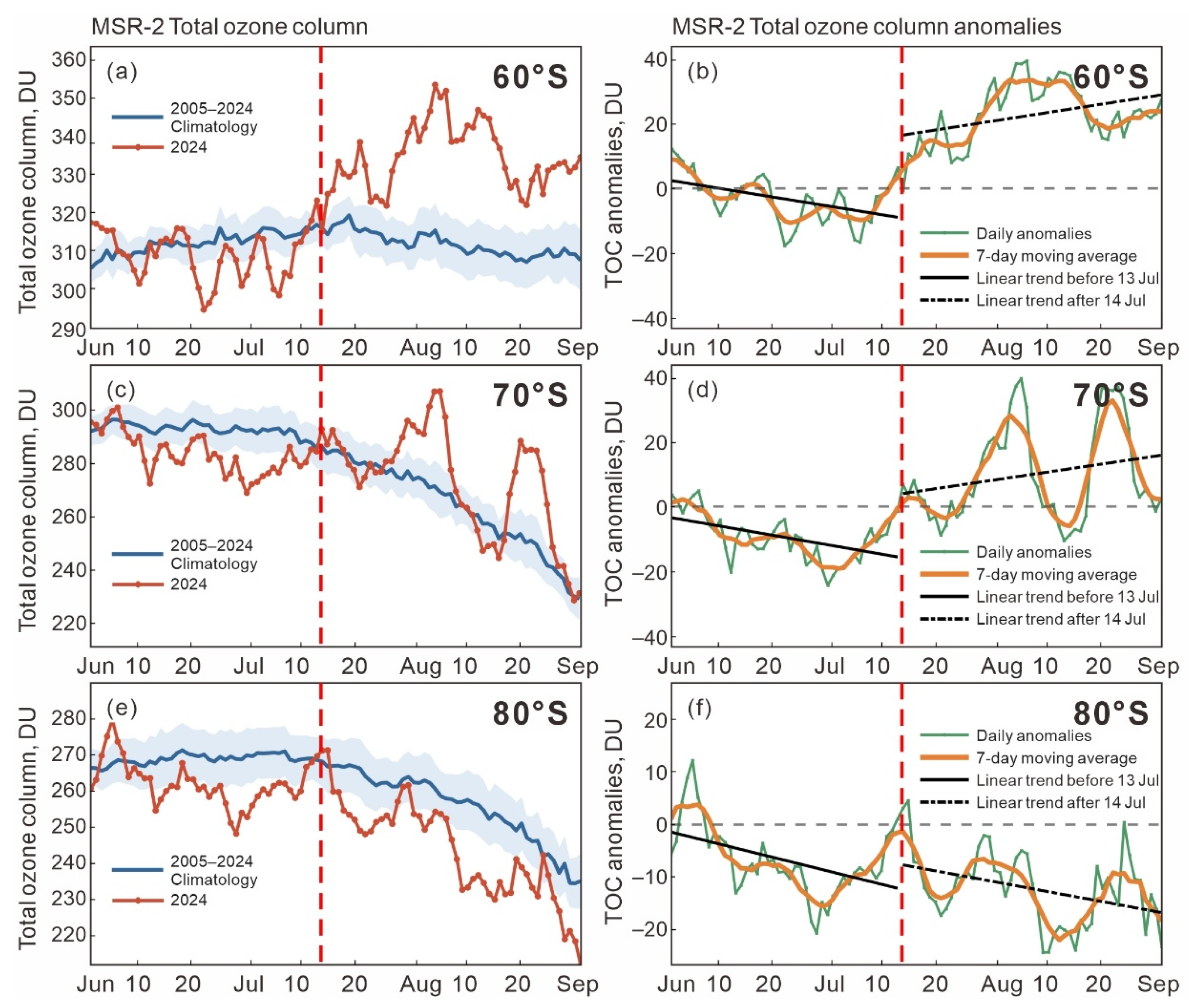
Figure 7 presents the latitudinal structure and temporal evolution of the total ozone column (TOC) and its anomalies across 60°S, 70°S, and 80°S during the 2024 austral winter, with the red dashed line marking 13 July 2024—a key transition point associated with the 2024 Southern Hemisphere sudden stratospheric warming (SSW). Figure 7a,c,e show the absolute TOC values, revealing a striking latitudinal divergence after mid-July. At 60°S, TOC rises sharply above the climatological mean, peaking at ~355 DU in mid-August, indicating significant ozone enrichment. At 70°S, TOC shows a transient peak around early August (~305 DU) before declining sharply to ~230 DU by early September. At 80°S, TOC declines steadily after mid-July, reaching ~210 DU by early September, well below the climatological baseline. This creates a pronounced poleward gradient in the ozone response, where the outer polar vortex region (60°S) exhibits ozone accumulation while the inner vortex core (80°S) experiences sustained ozone depletion, with 70°S representing an intermediate, transitional behavior.
Figure 7.
Zonal-mean daily total ozone column (TOC) and TOC absolute anomalies at 60°S, 70°S and 80°S during austral JJA 2024, derived from the MSR-2 reanalysis. Left panels (a,c,e) display daily TOC; red curves represent 2024 daily values, blue curves denote the 2005–2024 climatology with light blue shading for the 95% confidence interval. Right panels (b,d,f) show TOC anomalies at each latitude relative to the 2005–2024 climatology at that latitude. Green lines are raw daily anomalies; orange lines are the Seven-day moving average. Two segmented linear trends are fitted separately: solid black lines represent linear trends before 13 July, black dash-dot lines represent linear trends starting from 14 July to 31 August, and gray dashed lines mark the zero line.
In Figure 7b,d,f present TOC anomalies alongside segmented linear trends before and after 13 July, quantifying the dynamical transition linked to the SSW. Prior to 13 July, all three latitudes show negative TOC anomalies and consistent downward trends: −0.27 to −0.28 DU day−1 at 60–70°S and −0.25 DU day−1 at 80°S, consistent with a strengthened polar vortex that traps ozone-poor polar air and suppresses poleward transport of ozone-rich midlatitude air. After 14 July, the trends reverse dramatically at 60°S and 70°S, shifting to positive rates of +0.26 DU day−1 and +0.23 DU day−1, respectively, driving anomalies from negative to positive. Meanwhile, 80°S retains a weakened negative trend (−0.19 DU day−1), indicating a delayed recovery. This latitudinal asymmetry arises from SSW-induced dynamical changes: the weakened polar vortex and enhanced planetary wave activity promote the poleward transport of ozone-enriched air to 60–70°S, while the more isolated inner vortex at 80°S lags in circulation adjustment, sustaining negative ozone anomalies through limited ozone replenishment. These results quantitatively demonstrate that the 2024 SSW played a pivotal role in reshaping the stratospheric ozone distribution via modified meridional transport and vortex dynamics. The 13 July breakpoint is used as the reference date because it marks the first warming peak of the event, and not because it is a statistically optimal breakpoint; the fits are based on unsmoothed daily anomalies.
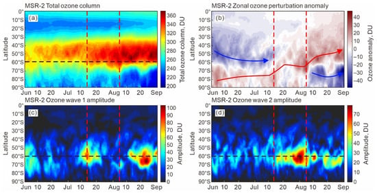
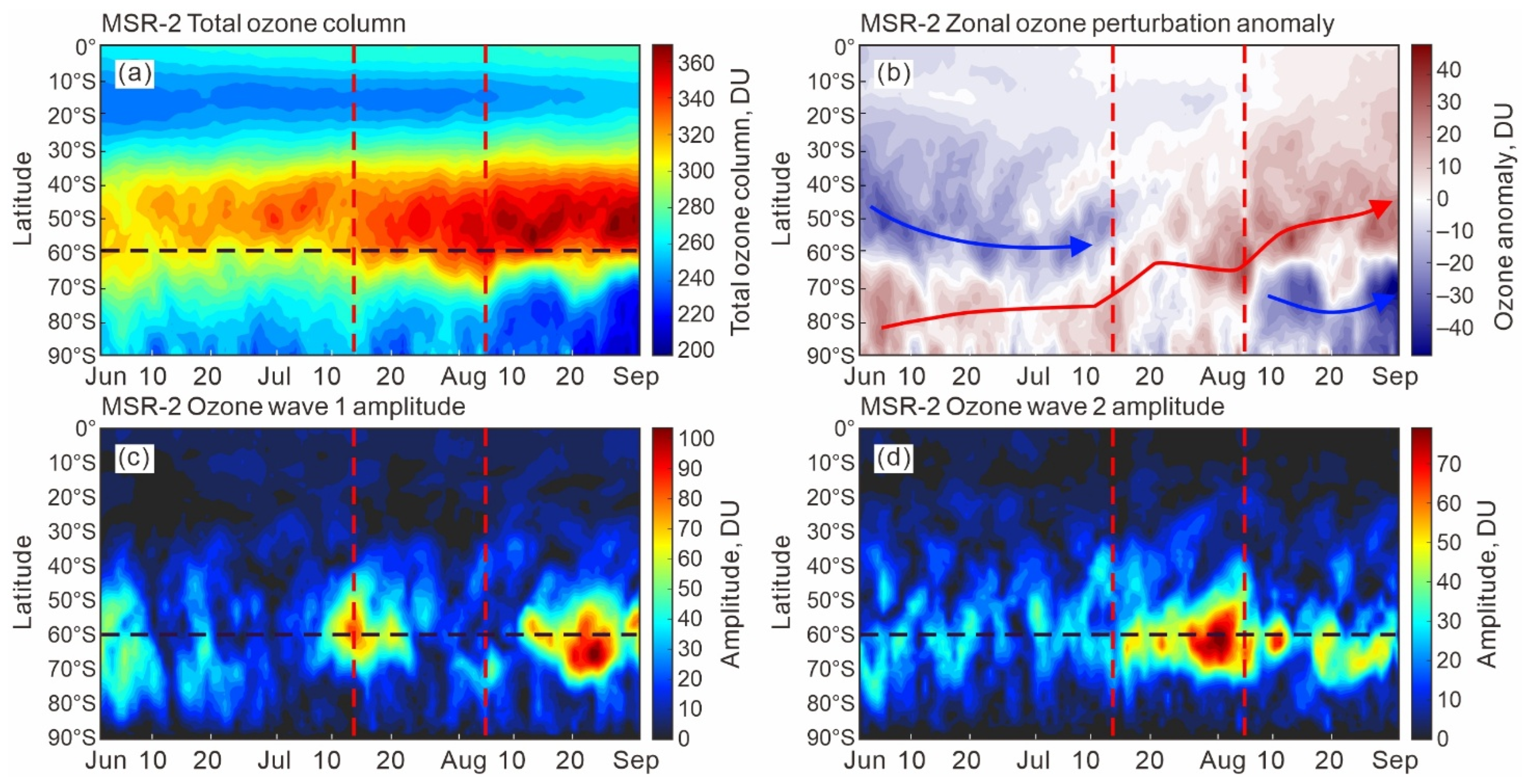
The latitude–time cross-section of total ozone column over the Southern Hemisphere during June–August 2024, revealing a pronounced meridional gradient in ozone distribution, is presented in Figure 8a. Ozone concentrations peak at mid-latitudes (30–50°S), reaching approximately 340–360 Dobson Units (DU), while values decline sharply poleward, dropping to 200–260 DU south of 60°S. This persistent pattern reflects the climatological mid-latitude ozone maximum and polar ozone depletion, with a stable band of enhanced ozone (280–340 DU) maintained across 30–60°S throughout the period. The gradual weakening of this poleward gradient in late August suggests a disruption of the meridional transport regime, likely linked to the dynamical perturbations associated with the 2024 Antarctic SSW.
Figure 8.
(a) Latitude–time cross-section of total ozone column (DU) over the Southern Hemisphere during June–August (JJA) 2024, based on MSR-2 data; (b) zonal-mean ozone perturbation anomaly, computed relative to the daily climatology of the Southern Hemisphere zonal mean, with arrows indicating the equatorward migration of positive anomalies and the poleward migration of negative anomalies; (c,d) amplitudes of zonal ozone wave 1 and wave 2. The dashed horizontal line marks 60°S, and the vertical dashed lines indicate dates of extremely high temperatures.
Figure 8b illustrates the zonal mean ozone perturbation anomaly, capturing the wave-driven redistribution of ozone during the SSW. Before the SSW, ozone anomalies were negative at lower latitudes (equatorward of 60°S) and positive at higher latitudes (poleward of 60°S). After 5 August, the pattern reversed: positive anomalies appeared at lower latitudes and negative anomalies at higher latitudes. This opposing migration of anomalies reveals a clear meridional rearrangement of ozone, with positive anomalies migrating equatorward (from 50–60°S to 40–50°S) and negative anomalies advancing poleward (toward 70–80°S). This description refers to the movement of anomaly patterns rather than to individual air-parcel trajectories. Figure 8c,d further show that zonal ozone wave 1 exhibits two prominent amplitude peaks (~80–100 DU) at 60–70°S around mid-July and late August, while ozone wave 2 reaches a sharp peak (~70 DU) at the same latitudes during early August, coinciding with the extreme temperature maxima marked by vertical dashed lines. The confinement of these wave amplitudes to 40–80°S—overlapping with the climatological polar vortex edge at 60°S—indicates that wave 1 and wave 2 are closely associated with the perturbation of the polar vortex and with the observed ozone redistribution via meridional mixing and transport. We note that the ozone anomalies in Figure 7f and Figure 8b are not constructed from the same reference field: those in Figure 7f are referred to a climatology at a single latitude, whereas those in Figure 8b are referred to a daily climatology averaged over a latitude band. The two panels are therefore not directly comparable at high southern latitudes.
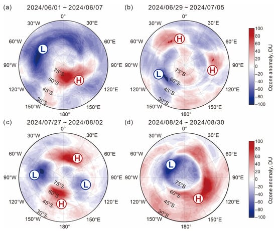
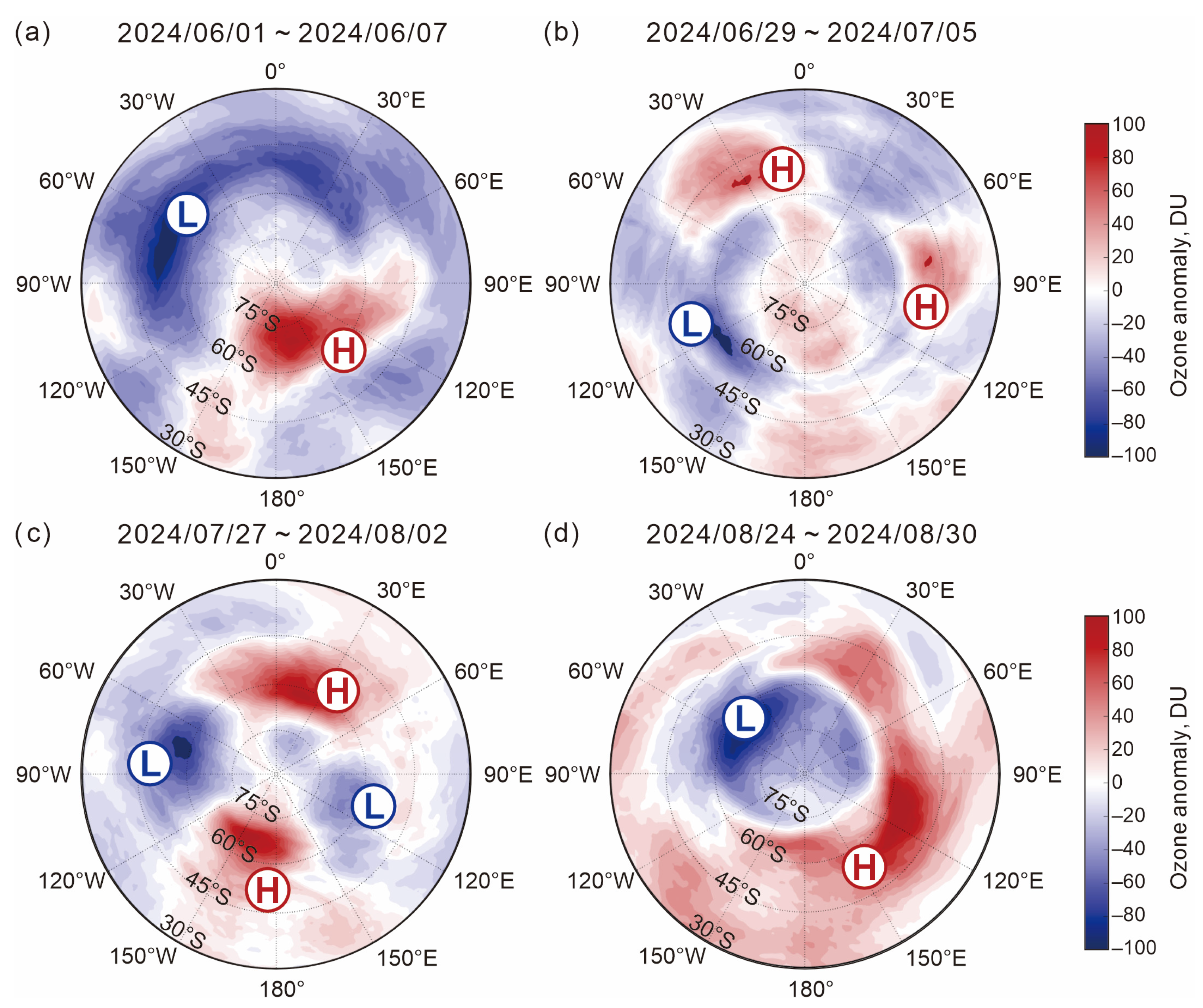
Figure 9 shows the Seven-day mean ozone perturbation distributions (unit: DU) during four typical periods in the 2024 Southern Hemisphere winter (June–August). From 1 to 7 June 2024, ozone anomalies exhibit a monopolar pattern, with significant positive anomalies (red, marked H) in the region of 60–90°S and 30°E–150°E, and strong negative anomalies (blue, marked L) near 60°W, forming a sharp contrast between mid-latitude negative and high-latitude positive anomalies. From 29 June to 5 July 2024, ozone anomalies transition into a bipolar structure, with two positive anomaly centers (H) near 30°W and 90°E, respectively, and a negative anomaly center (L) in the 90–120°W region, with positive and negative anomalies distributed alternately along the zonal direction. From 27 July to 2 August 2024, ozone anomalies present a multipolar distribution, with positive anomaly centers (H) near 30°E and 180°, and negative anomaly centers (L) near 60°W and 120°E, where high- and mid-latitude anomalies are nested, leading to a more complex structure. This location of ozone anomalies is associated with wave 2 domination that reached its peak in early August (Figure 8d). From 24 to 30 August 2024, ozone anomalies show a vortex-like pattern, with a strong negative anomaly center (L) in the 60°W–0° region and a strong positive anomaly center (H) near 90°E, forming a zonal ring wave train of positive and negative anomalies, reflecting the modulation of planetary-scale waves on ozone distribution.
Figure 9.
The Seven-day mean (a) 1–7 June 2024; (b) 29 June–5 July 2024; (c) 27 July–2 August 2024; (d) 24–30 August ozone perturbation distributions (unit: DU) during four typical periods in the 2024 Southern Hemisphere winter.
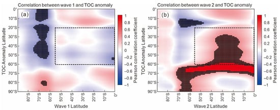
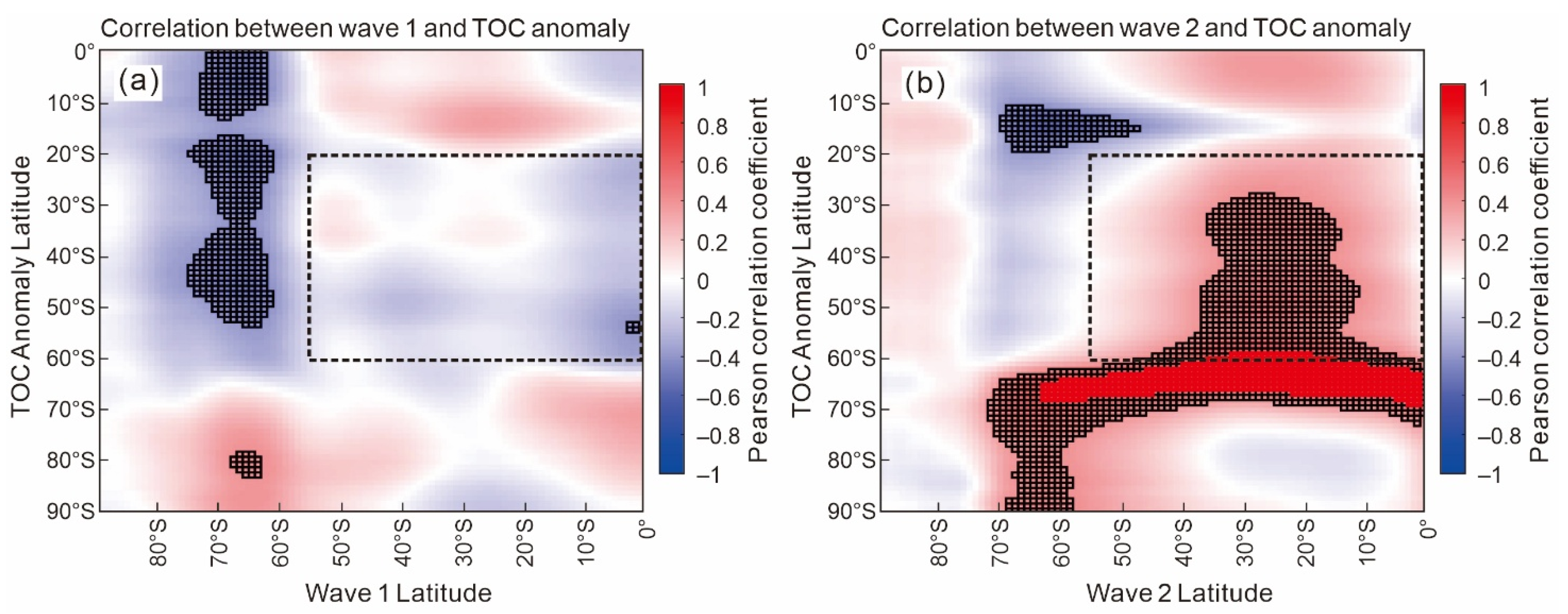
Figure 10 shows the cross-latitudinal Pearson correlation distributions between planetary wave 1 and wave 2 amplitudes and zonal-mean TOC anomalies over the Southern Hemisphere. In the left panel, the wave 1 amplitude at 60–70°S is negatively correlated with zonal-mean TOC anomalies over 0–50°S, with correlation coefficients between −0.6 and −0.4. The correlations are weak (|R| < 0.4) at all other latitudes. In the right panel, wave 2 amplitudes over 0–65°S show strong positive correlations (R ≥ 0.6) with TOC anomalies in the 60–70°S band. The regions of significant correlation for the two waves overlap only slightly. Within the boxed region (20–60°S), TOC anomalies are negatively correlated with the wave 1 amplitude and positively correlated with the wave 2 amplitude.
Figure 10.
Cross-latitudinal Pearson correlation distribution between the amplitudes of (a) wave 1 and (b) wave 2 and the zonal-mean TOC anomalies in the Southern Hemisphere during June–August 2024. The dashed black rectangle marks the 20–60°S band, where wave 1 shows negative correlation with TOC while wave 2 shows positive correlation, illustrating the wave-type selectivity of wave–ozone coupling. Stippling denotes points significant at the 95% level from a two-tailed t-test in which the effective sample size is reduced for lag-1 autocorrelation.
The two waves therefore exhibit clear wave-type and latitudinal selectivity in their coupling with ozone. Wave 1 dominates the negative coupling over 0–50°S (low-to-midlatitudes), whereas wave 2 governs the positive coupling over the 60–70°S polar collar region. The limited spatial overlap between the two correlation patterns suggests that the two waves are associated with largely separable correlation structures. The opposite correlation signs within the same latitude band further indicate a possible temporal offset between the two wave forcings, consistent with the sequential amplification of wave 1 in early July and wave 2 in late July. Wave 2 thus shows a positive correlation with TOC anomalies in the 60–70°S polar collar during the 2024 SSW.
4. Discussion
The 2024 austral winter witnessed an event without precedent in the satellite era: two successive minor Antarctic sudden stratospheric warmings occurring in July–August, the earliest midwinter SSWs ever recorded over the Southern Hemisphere. While prior studies have established the tropospheric blocking, sea-ice loss, stratospheric preconditioning, and downward SAM propagation as the triggering chain for these events [34,35], several critical aspects of the wave forcing and ozone response remain unresolved. Zi et al. [34] diagnosed the tropospheric blocking–planetary wave cascade that triggered the first 2024 warming, decomposing the eddy heat flux into its climatological, linear and nonlinear terms, resolving the nonlinear term by wavenumber at 10 and 100 hPa, and complementing this with EP flux divergence, potential-vorticity-gradient preconditioning and Antarctic sea-ice diagnostics. They identified the nonlinear wave–wave interaction, rather than the linear interaction between anomalous and climatological waves, as the dominant contribution at 45–75°S, and examined the ozone response as a polar-cap average (60–90°S), attributing it to an intensified residual meridional circulation. Lim et al. [35] placed the same event in the context of wintertime Southern Hemisphere stratospheric variability over 1979–2023, diagnosed the leading mode of the 1 hPa winter jet as a meridional expansion or contraction of the vortex, and quantified the associated wave forcing through wavenumber-resolved poleward eddy heat and momentum fluxes, reporting a record July wavenumber-2 heat flux at 100 hPa, a record contraction of the vortex for July, a polar-cap total ozone column anomaly for the event of about +1σ, and the record negative Southern Annular Mode values of early August 2024. Neither diagnostic set resolves the vertical structure of wavenumber-specific wave activity between the lower stratosphere and the stratopause, and a polar-cap average by construction removes the latitudinal structure of the ozone response. The present study addresses both gaps. First, we provide a quantitative, stage-separated diagnosis of wave 1 and wave 2 forcing across the full 20–50 km altitude range using multiple independent datasets, demonstrating that the two warming peaks were associated with distinct wave components having different vertical structures.
The finding that wave 1 and wave 2 operate in a temporally staggered, functionally distinct manner during the 2024 SSW carries implications beyond this single event. In Northern Hemisphere major SSWs, wave 1 is generally considered the primary forcing agent, with wave 2 playing a secondary role primarily during vortex-splitting events [12,46]. Our results suggest that in the Southern Hemisphere, where the polar vortex is typically more zonally symmetric and less receptive to wave forcing, the relative contribution of wave 2 may be disproportionately important for achieving the threshold of vortex disruption. The delayed but vertically extensive enhancement of wave 2 observed in late July–early August (Figure 5b), peaking in the 25–35 km layer, suggests that wave 2 amplification was not merely a passive response to vortex weakening but contributed to sustaining the second warming phase. This is consistent with the resonance amplification mechanism proposed by [36], wherein stratospheric preconditioning by the first warming episode creates a refractive index structure favorable for subsequent wave 2 growth. Notably, Zi et al. [34] reported wave 1 and wave 2 amplitudes near historical extremes at 10 hPa but did not examine their vertical distribution; our vertically resolved analysis reveals that the two wave components reached their respective maxima at different altitudes and during different phases, a distinction that a single-level diagnostic cannot capture. We also note that amplitude and eddy heat flux need not peak simultaneously: the record-breaking wave-2 activity in July reported by Lim et al. [35] is diagnosed from the eddy heat flux, which peaks earlier than the 10 hPa geopotential height amplitude, so the two diagnostics are consistent rather than contradictory.
Aura MLS employs limb sounding with sparse, non-uniform longitudinal sampling, and interpolating its geopotential height onto a regular 360-point longitude grid before the Fourier analysis can, in principle, alias the wave 1 and wave 2 patterns. This is precisely why MERRA-2 and ERA5 are used as the primary datasets for the wave amplitude analysis (Figure 3 and Figure 4), while MLS is used only for the vertical structure validation of Figure 5. The correlations between MLS and the reanalysis wave amplitudes at 60°S and 10 hPa are high (R > 0.94 for both wave 1 and wave 2; Figure S2), which indicates that the MLS sampling aliasing does not significantly distort the wave signal at 60°S during this event.
The wave–ozone coupling selectivity revealed by our cross-latitudinal correlation analysis (Figure 10) represents a novel observational result with implications for understanding Antarctic ozone variability under a changing climate. Whereas Zi et al. [34] reported a bulk ozone increase averaged over 60–90°S and attributed it to residual meridional circulation transport, our latitude-resolved analysis uncovers a more nuanced picture. Wave 1 amplitudes at 60–70°S are negatively correlated with zonal-mean TOC anomalies over 0–50°S, with correlation coefficients of −0.4 to −0.6. In contrast, wave 2 amplitudes over 0–65°S are positively correlated with TOC anomalies in the 60–70°S band, with R ≥ 0.6. These correlation structures are latitudinally separated, which is consistent with two partially separable transport pathways. The poleward progression of negative ozone anomalies and equatorward migration of positive anomalies (Figure 8b) are qualitatively consistent with the two-cell residual circulation response described in observational MLS analyses of the 2009 Arctic major warming [47], though the quantitative attribution of this response to specific wave components warrants further investigation using transformed Eulerian-mean diagnostics. We further note that the positive correlation for wave 2 concerns the 60–70°S collar, which lies equatorward of the polar cap; the abnormally southward ozone response described by Lim et al. [35], with maxima near 50°S and no significant anomalies over the polar cap, is consistent with a positive anomaly in the collar rather than over the cap.
Several limitations should be acknowledged. First, our analysis relies on reanalysis and satellite data over a single season, which limits the statistical robustness of the correlation-based ozone attribution. The extreme rarity of Antarctic winter SSWs precludes a large-sample statistical approach; however, the consistency across independent datasets strengthens confidence in the identified relationships. Second, we did not carry out a residual-mean (transformed Eulerian-mean) circulation diagnosis, which would quantify the Brewer–Dobson circulation response directly; such a diagnosis is beyond the scope of this observational analysis and is identified as a target for future work. Third, the potential modulating roles of the quasi-biennial oscillation (QBO) and El Niño–Southern Oscillation (ENSO) on the 2024 event were not assessed. The QBO was in its easterly phase during austral winter 2024, a configuration previously linked to increased susceptibility to SSW onset via modified wave propagation conditions [48,49], and this may have contributed to the unusual preconditioning of the 2024 Antarctic stratosphere. Zi et al. [34] similarly did not account for these tropical forcings, underscoring a shared limitation that future studies should address. Fourth, our ozone analysis focused on total column amounts and did not separate dynamical from chemical contributions to ozone changes; heterogeneous chemical ozone depletion may remain competitive with transport effects, particularly at high latitudes within the cold vortex core. Future work incorporating trajectory analysis, ozone tendency budgets, and chemistry–climate model simulations would help disentangle these processes.
The 2024 event challenges the canonical view that Antarctic winter SSWs are suppressed by the persistent austral polar night jet. The fact that two successive warmings occurred during midwinter, rather than in late winter or spring as in previous events (1988, 2002, 2019), raises the question of whether the conditions favoring Southern Hemisphere SSWs are evolving under climate change. Rising greenhouse gas concentrations induce stratospheric cooling—which strengthens the polar vortex—but also enhance tropospheric wave generation through changes in tropical sea surface temperatures and Hadley cell expansion [50]. These competing influences create uncertainty in projections of future Antarctic SSW frequency. The 2024 event provides a valuable observational benchmark for evaluating the fidelity of climate models in simulating extreme stratospheric variability under both present-day and future climate forcing. If the preconditioning mechanisms identified here—including tropospheric blocking, stratospheric wave resonance, and wave–ozone feedback—are captured by models, improved seasonal prediction of Antarctic stratospheric extremes and their surface impacts may become feasible.
5. Conclusions
This study provides a systematic observational diagnosis of the unprecedented pair of successive midwinter Antarctic sudden stratospheric warmings in July–August 2024, with a focus on the stage-separated planetary wave forcing and the associated wave–ozone coupling. The principal findings are summarized as follows:
- The 2024 Antarctic winter witnessed two consecutive minor SSWs, the earliest winter warmings recorded over Antarctica in the satellite era, characterized by a maximum reduction of approximately 23% in the 10 hPa zonal-mean wind at 60°S (from ~74 m s−1 on 13 July to ~57 m s−1 on 5 August), and polar temperature anomalies of approximately 15 K and 17 K above the 1979–2024 climatological mean at the 13 July and 5 August peaks, respectively. These events were driven by an anomalously strong upward propagation of tropospheric planetary waves that deposited westward momentum in the stratosphere and systematically weakened the polar night jet.
- Wave 1 and wave 2 exerted stage-separated, functionally distinct forcing on the polar vortex. Wave 1 dominated the first warming peak in mid-July, with vertically coherent amplitude maxima spanning 20–50 km and peak geopotential height amplitudes exceeding 1750 m near 40 km. Wave 2 amplification, concentrated in the 25–35 km layer during late July–early August, was closely associated with the second, more intense phase of vortex disruption. Multi-dataset analysis indicates that the sequential enhancement of wave 1 and wave 2 activity is closely associated with the two-stage evolution of the 2024 Antarctic SSW.
- A clear wave-type and latitude-selective coupling between planetary wave activity and stratospheric ozone redistribution is established. Wave 1 exhibits a significant negative correlation with total ozone column anomalies across the 0–50°S low-to-midlatitude band, reflecting the equatorward export of ozone-poor air during the warming onset. In contrast, wave 2 shows strong positive coupling with TOC over the 60–70°S polar collar region, consistent with the poleward transport of ozone-rich air. These two pathways display limited latitudinal overlap, indicating partially separable correlation structures for stratospheric ozone distribution during Antarctic SSWs. The segmented linear trend analysis confirms a dynamical transition on ~13 July, after which TOC trends reversed from negative (−0.27 DU day−1) to positive (+0.26 DU day−1) at 60°S, coinciding with the peak warming period.
- The wave-forced ozone anomalies exhibit a progressive meridional reorganization, with positive anomalies migrating equatorward from 50–60°S to 40–50°S and negative anomalies advancing poleward toward 70–80°S, consistent with a perturbed BDC and enhanced planetary-wave-driven meridional mixing across the polar vortex edge.
These results demonstrate that the 2024 Antarctic SSW provides a unique natural laboratory for investigating stratosphere–troposphere dynamical coupling and wave–ozone interactions under conditions of extreme planetary wave forcing. The identified wave-type selectivity in ozone transport carries implications for understanding Antarctic ozone variability, stratospheric predictability, and the potential modulation of ozone hole development by dynamical extremes in a changing climate.
Supplementary Materials
The following supporting information can be downloaded at: https://www.mdpi.com/article/10.3390/rs18213741/s1.
Author Contributions
Conceptualization, Y.S. and F.Y.; data curation, Y.S. and F.Y.; formal analysis, Y.S., A.G. and G.M.; investigation, Y.S., D.Z. and G.M.; methodology, Y.S.; project administration, G.M.; software, Y.S. and F.Y.; supervision, G.M. and A.G.; validation, Y.S. and D.Z.; visualization, Y.S. and F.Y.; writing—original draft, Y.S. and F.Y.; writing—review and editing, Y.S., G.M., D.Z. and A.G. Each author contributed to the interpretation and discussion of the results and edited the manuscript. All authors have read and agreed to the published version of the manuscript.
Funding
This research was funded by Heilongjiang University, Harbin, China, grant number 2025-KYYWF-ZR0422.
Data Availability Statement
The data used in this study are available from the following archives: MERRA-2, NASA Global Modeling and Assimilation Office (GMAO)/GES DISC, https://gmao.gsfc.nasa.gov/reanalysis/MERRA-2/, accessed 15 September 2026; ERA5 hourly pressure-level data, Copernicus Climate Data Store (CDS), https://cds.climate.copernicus.eu/ (https://doi.org/10.24381/cds.bd0915c6), accessed 15 September 2026; Aura MLS, NASA JPL Microwave Limb Sounder, https://mls.jpl.nasa.gov/, accessed 15 September 2026; MSR-2 total ozone column, KNMI TEMIS, https://www.temis.nl/protocols/O3global.php (https://doi.org/10.21944/temis-ozone-msr2), accessed 15 September 2026. The analysis scripts that reproduce all figures are available from the corresponding author on request.
Acknowledgments
This work was partially supported by Heilongjiang University, Harbin, China, by College of Physics, International Center of Future Science, Jilin University, China (the project DH20260025), and by the Taras Shevchenko National University of Kyiv, Ukraine (the project 0126U004808). This study contributed to the State Institution National Antarctic Scientific Center, Ukraine, research objectives. We acknowledge data availability from Modern-Era Retrospective analysis for Research and Applications, Version 2 (MERRA-2) reanalysis (https://gmao.gsfc.nasa.gov/gmao-products/merra-2/, accessed on 10 July 2026), Microwave Limb Sounder (Aura MLS) satellite observations (https://mls.jpl.nasa.gov/, accessed on 4 August 2026) and the Multi-Sensor Reanalysis version 2 (MSR-2) total ozone product data (https://www.temis.nl/protocols/O3global.php, accessed on 15 July 2026). Ozone concentration and air temperature at selected pressure levels are derived from the European Centre for Medium-Range Weather Forecasts (ECMWF) ERA5 dataset (https://cds.climate.copernicus.eu/datasets/reanalysis-era5-pressure-levels?tab=overview, accessed on 20 June 2026).
Conflicts of Interest
The authors declare no conflicts of interest.
Abbreviations
The following abbreviations are used in this manuscript:
| BDC | Brewer–Dobson Circulation |
| C3S | Copernicus Climate Change Service |
| DU | Dobson Units |
| ERA5 | ECMWF Reanalysis Version 5 |
| KNMI | Royal Netherlands Meteorological Institute |
| MLS | Aura Microwave Limb Sounder |
| MSR-2 | Multi-Sensor Reanalysis Version 2 |
| NH | Northern Hemisphere |
| SH | Southern Hemisphere |
| SSW | Sudden Stratospheric Warming |
| TOC | Total Ozone Column |
| WOUDC | World Ozone and Ultraviolet Radiation Data Centre |
References
- Haynes, P. Stratospheric Dynamics. Annu. Rev. Fluid Mech. 2005, 37, 263–293. [Google Scholar] [CrossRef] [Scilit]
- Waugh, D.W.; Sobel, A.H.; Polvani, L.M. What Is the Polar Vortex and How Does It Influence Weather? Bull. Am. Meteorol. Soc. 2017, 98, 37–44. [Google Scholar] [CrossRef] [Scilit]
- Butchart, N. The Brewer–Dobson Circulation. Rev. Geophys. 2014, 52, 157–184. [Google Scholar] [CrossRef] [Scilit]
- Butler, A.H.; Seidel, D.J.; Hardiman, S.C.; Butchart, N.; Birner, T.; Match, A. Defining Sudden Stratospheric Warmings. Bull. Am. Meteorol. Soc. 2015, 96, 1913–1928. [Google Scholar] [CrossRef] [Scilit]
- Baldwin, M.P.; Ayarzagüena, B.; Birner, T.; Butchart, N.; Butler, A.H.; Charlton-Perez, A.J.; Domeisen, D.I.V.; Garfinkel, C.I.; Garny, H.; Gerber, E.P.; et al. Sudden Stratospheric Warmings. Rev. Geophys. 2021, 59, e2020RG000708. [Google Scholar] [CrossRef] [Scilit]
- Matsuno, T. A Dynamical Model of the Stratospheric Sudden Warming. J. Atmos. Sci. 1971, 28, 1479–1494. [Google Scholar] [CrossRef] [Scilit]
- Andrews, D.G.; Holton, J.R.; Leovy, C.B. Middle Atmosphere Dynamics; Academic Press: Orlando, FL, USA, 1987; Available online: https://www.sciencedirect.com/bookseries/international-geophysics/vol/40 (accessed on 10 August 2026).
- Shi, G.; Krochin, W.; Sauvageat, E.; Stober, G. Ozone Anomalies over the Polar Regions during Stratospheric Warming Events. Atmos. Chem. Phys. 2024, 24, 10187–10207. [Google Scholar] [CrossRef] [Scilit]
- Baldwin, M.P.; Thompson, D.W.J. A Critical Comparison of Stratosphere–Troposphere Coupling Indices. Q. J. R. Meteorol. Soc. 2009, 135, 1661–1672. [Google Scholar] [CrossRef] [Scilit]
- Domeisen, D.I.V.; Grams, C.M.; Papritz, L. The Role of North Atlantic–European Weather Regimes in the Surface Impact of Sudden Stratospheric Warming Events. Weather Clim. Dyn. 2020, 1, 373–388. [Google Scholar] [CrossRef] [Scilit]
- White, I.P.; Garfinkel, C.I.; Gerber, E.P.; Jucker, M.; Aquila, V.; Oman, L.D. The Downward Influence of Sudden Stratospheric Warmings: Association with Tropospheric Precursors. J. Clim. 2019, 32, 85–108. [Google Scholar] [CrossRef] [Scilit] [PubMed]
- Wang, Y.; Shulga, V.; Milinevsky, G.; Patoka, A.; Evtushevsky, O.; Klekociuk, A.; Han, W.; Grytsai, A.; Shulga, D.; Myshenko, V.; et al. Winter 2018 Major Sudden Stratospheric Warming Impact on Midlatitude Mesosphere from Microwave Radiometer Measurements. Atmos. Chem. Phys. 2019, 19, 10303–10317. [Google Scholar] [CrossRef] [Scilit]
- Charlton, A.J.; Polvani, L.M.; Perlwitz, J.; Sassi, F.; Manzini, E.; Shibata, K.; Pawson, S.; Nielsen, E.; Rind, D. A New Look at Stratospheric Sudden Warmings. Part II: Evaluation of Numerical Model Simulations. J. Clim. 2007, 20, 470–488. [Google Scholar] [CrossRef] [Scilit]
- Lim, E.-P.; Hendon, H.H.; Thompson, D.W.J. Seasonal Evolution of Stratosphere-Troposphere Coupling in the Southern Hemisphere and Implications for the Predictability of Surface Climate. J. Geophys. Res. Atmos. 2018, 123, 12002–12016. [Google Scholar] [CrossRef] [Scilit]
- Kuroda, Y.; Kodera, K. Interannual Variability in the Troposphere and Stratosphere of the Southern Hemisphere Winter. J. Geophys. Res. Atmos. 1998, 103, 13787–13799. [Google Scholar] [CrossRef] [Scilit]
- Charney, J.G.; Drazin, P.G. Propagation of Planetary-Scale Disturbances from the Lower into the Upper Atmosphere. J. Geophys. Res. 1961, 66, 83–109. [Google Scholar] [CrossRef] [Scilit]
- Martius, O.; Polvani, L.M.; Davies, H.C. Blocking Precursors to Stratospheric Sudden Warming Events. Geophys. Res. Lett. 2009, 36, L14806. [Google Scholar] [CrossRef] [Scilit]
- Woollings, T.; Charlton-Perez, A.; Ineson, S.; Marshall, A.G.; Masato, G. Associations between Stratospheric Variability and Tropospheric Blocking. J. Geophys. Res. Atmos. 2010, 115, D06108. [Google Scholar] [CrossRef] [Scilit]
- Charlton, A.J.; O’Neill, A.; Lahoz, W.A.; Berrisford, P. The Splitting of the Stratospheric Polar Vortex in the Southern Hemisphere, September 2002: Dynamical Evolution. J. Atmos. Sci. 2005, 62, 590–602. [Google Scholar] [CrossRef] [Scilit]
- Newman, P.A.; Nash, E.R. The Unusual Southern Hemisphere Stratosphere Winter of 2002. J. Atmos. Sci. 2005, 62, 614–628. [Google Scholar] [CrossRef] [Scilit]
- Sinnhuber, B.-M.; Weber, M.; Amankwah, A.; Burrows, J.P. Total Ozone during the Unusual Antarctic Winter of 2002. Geophys. Res. Lett. 2003, 30, 1580. [Google Scholar] [CrossRef] [Scilit]
- Varotsos, C. The Southern Hemisphere Ozone Hole Split in 2002. Environ. Sci. Pollut. Res. 2002, 9, 375–376. [Google Scholar] [CrossRef] [Scilit] [PubMed]
- Kanzawa, H.; Kawaguchi, S. Large Stratospheric Sudden Warming in Antarctic Late Winter and Shallow Ozone Hole in 1988. Geophys. Res. Lett. 1990, 17, 77–80. [Google Scholar] [CrossRef] [Scilit]
- Shen, X.; Wang, L.; Osprey, S. Tropospheric Forcing of the 2019 Antarctic Sudden Stratospheric Warming. Geophys. Res. Lett. 2020, 47, e2020GL089343. [Google Scholar] [CrossRef] [Scilit]
- Hio, Y.; Yoden, S. Interannual Variations of the Seasonal March in the Southern Hemisphere Stratosphere for 1979–2002 and Characterization of the Unprecedented Year 2002. J. Atmos. Sci. 2005, 62, 567–580. [Google Scholar] [CrossRef] [Scilit]
- Jucker, M. Are Sudden Stratospheric Warmings Generic? Insights from an Idealized GCM. J. Atmos. Sci. 2016, 73, 5061–5080. [Google Scholar] [CrossRef] [Scilit]
- Polvani, L.M.; Waugh, D.W. Upward Wave Activity Flux as a Precursor to Extreme Stratospheric Events and Subsequent Anomalous Surface Weather Regimes. J. Clim. 2004, 17, 3548–3554. [Google Scholar] [CrossRef] [Scilit]
- Kodera, K.; Mukougawa, H.; Fujii, A. Influence of the Vertical and Zonal Propagation of Stratospheric Planetary Waves on Tropospheric Blockings. J. Geophys. Res. Atmos. 2013, 118, 8333–8345. [Google Scholar] [CrossRef] [Scilit]
- Nishii, K.; Nakamura, H.; Orsolini, Y.J. Geographical Dependence Observed in Blocking High Influence on the Stratospheric Variability through Enhancement and Suppression of Upward Planetary-Wave Propagation. J. Clim. 2011, 24, 6408–6423. [Google Scholar] [CrossRef] [Scilit]
- McIntyre, M.E.; Palmer, T.N. The “Surf Zone” in the Stratosphere. J. Atmos. Terr. Phys. 1984, 46, 825–849. [Google Scholar] [CrossRef] [Scilit]
- Takaya, K.; Nakamura, H. A Formulation of a Phase-Independent Wave-Activity Flux for Stationary and Migratory Quasigeostrophic Eddies on a Zonally Varying Basic Flow. J. Atmos. Sci. 2001, 58, 608–627. [Google Scholar] [CrossRef] [Scilit]
- Colucci, S.J.; Kelleher, M.E. Diagnostic Comparison of Tropospheric Blocking Events with and without Sudden Stratospheric Warming. J. Atmos. Sci. 2015, 72, 2227–2240. [Google Scholar] [CrossRef] [Scilit]
- Simpson, I.R.; Blackburn, M.; Haigh, J.D. The Role of Eddies in Driving the Tropospheric Response to Stratospheric Heating Perturbations. J. Atmos. Sci. 2009, 66, 1347–1365. [Google Scholar] [CrossRef] [Scilit]
- Zi, Y.; Long, Z.; Sheng, J.; Lu, G.; Perrie, W.; Xiao, Z. The Sudden Stratospheric Warming Events in the Antarctic in 2024. Geophys. Res. Lett. 2025, 52, e2025GL115257. [Google Scholar] [CrossRef] [Scilit]
- Lim, E.-P.; Thompson, D.W.J.; Butler, A.H.; Wheeler, M.C.; Nakamura, H.; Jucker, M.; Arblaster, J.M.; Hendon, H.H.; Newman, P.A.; Coy, L. Characteristics of Antarctic Stratospheric Variability During Winter: A Case Study of the 2024 Sudden Stratospheric Warming and Its Surface Impacts. J. Geophys. Res. Atmos. 2025, 130, e2025JD045089. [Google Scholar] [CrossRef] [Scilit]
- Albers, J.R.; Birner, T. Vortex Preconditioning due to Planetary and Gravity Waves prior to Sudden Stratospheric Warmings. J. Atmos. Sci. 2014, 71, 4028–4054. [Google Scholar] [CrossRef] [Scilit]
- Jucker, M.; Reichler, T. Dynamical Precursors for Statistical Prediction of Stratospheric Sudden Warming Events. Geophys. Res. Lett. 2018, 45, 13124–13132. [Google Scholar] [CrossRef] [Scilit]
- Hartmann, D.L.; Mechoso, C.R.; Yamazaki, K. Observations of Wave-Mean Flow Interaction in the Southern Hemisphere. J. Atmos. Sci. 1984, 41, 351–362. [Google Scholar] [CrossRef] [Scilit][Green Version]
- Hio, Y.; Yoden, S. Quasi-Periodic Variations of the Polar Vortex in the Southern Hemisphere Stratosphere due to Wave-Wave Interaction. J. Atmos. Sci. 2004, 61, 2510–2527. [Google Scholar] [CrossRef] [Scilit]
- Seviour, W.J.M.; Hardiman, S.C.; Gray, L.J.; Butchart, N.; MacLachlan, C.; Scaife, A.A. Skillful Seasonal Prediction of the Southern Annular Mode and Antarctic Ozone. J. Clim. 2014, 27, 7462–7474. [Google Scholar] [CrossRef] [Scilit]
- Zambri, B.; Solomon, S.; Thompson, D.W.J.; Fu, Q. Emergence of Southern Hemisphere Stratospheric Circulation Changes in Response to Ozone Recovery. Nat. Geosci. 2021, 14, 638–644. [Google Scholar] [CrossRef] [Scilit]
- Lim, E.-P.; Hendon, H.H.; Butler, A.H.; Thompson, D.W.J.; Lawrence, Z.D.; Scaife, A.A.; Shepherd, T.G.; Polichtchouk, I.; Nakamura, H.; Kobayashi, C.; et al. The 2019 Southern Hemisphere Stratospheric Polar Vortex Weakening and Its Impacts. Bull. Am. Meteorol. Soc. 2021, 102, E1150–E1171. [Google Scholar] [CrossRef] [Scilit]
- Yu, R.; Grytsai, A.; Milinevsky, G.; Evtushevsky, O.; Yukhymchuk, Y.; Zazubyk, D.; Klekociuk, A. Comparison of Antarctic Total Ozone Behavior in Pre-SSW, SSW, and Post-SSW Years. Ukr. Antarct. J. 2025, 23, 30–52. [Google Scholar] [CrossRef] [Scilit]
- de Laat, A.T.J.; Van Weele, M. The 2010 Antarctic Ozone Hole: Observed Reduction in Ozone Destruction by Minor Sudden Stratospheric Warmings. Sci. Rep. 2011, 1, 38. [Google Scholar] [CrossRef] [Scilit] [PubMed]
- van der A, R.J.; Allaart, M.A.F.; Eskes, H.J. Extended and refined multi sensor reanalysis of total ozone for the period 1970–2012. Atmos. Meas. Tech. 2015, 8, 3021–3035. [Google Scholar] [CrossRef] [Scilit]
- Matthewman, N.J.; Charlton, A.J.; Polvani, L.M. A New Look at Stratospheric Sudden Warmings. Part III: Polar Vortex Evolution and Vertical Structure. J. Clim. 2009, 22, 1566–1585. [Google Scholar] [CrossRef] [Scilit]
- Manney, G.L.; Schwartz, M.J.; Krüger, K.; Santee, M.L.; Pawson, S.; Lee, J.N.; Daffer, W.H.; Fuller, R.A.; Livesey, N.J. Aura Microwave Limb Sounder Observations of Dynamics and Transport During the Record-Breaking 2009 Arctic Stratospheric Major Warming. Geophys. Res. Lett. 2009, 36, L12815. [Google Scholar] [CrossRef] [Scilit]
- Holton, J.R.; Tan, H.-C. The Influence of the Equatorial Quasi-Biennial Oscillation on the Global Circulation at 50 mb. J. Atmos. Sci. 1980, 37, 2200–2208. [Google Scholar] [CrossRef] [Scilit]
- Anstey, J.A.; Shepherd, T.G. High-Latitude Influence of the Quasi-Biennial Oscillation. Q. J. R. Meteorol. Soc. 2014, 140, 1–21. [Google Scholar] [CrossRef] [Scilit]
- Jucker, M.; Reichler, T.; Waugh, D.W. How Frequent Are Antarctic Sudden Stratospheric Warmings in Present and Future Climate? Geophys. Res. Lett. 2021, 48, e2021GL093215. [Google Scholar] [CrossRef] [Scilit]

Disclaimer/Publisher’s Note: The statements, opinions and data contained in all publications are solely those of the individual author(s) and contributor(s) and not of MDPI and/or the editor(s). MDPI and/or the editor(s) disclaim responsibility for any injury to people or property resulting from any ideas, methods, instructions or products referred to in the content. |
© 2026 by the authors. Licensee MDPI, Basel, Switzerland. This article is an open access article distributed under the terms and conditions of the Creative Commons Attribution (CC BY) license.