GCDI: A Composite Drought Index on a 1-km Grid for China via Multi-Source Geo-Aware Feature Learning

Highlights

What are the main findings?

• GeoSPEI-1, constructed from neighboring station-based SPEI-1 values, provides the primary information source for GCDI-1 estimation, while multi-source environmental variables provide complementary information.
• Incorporating GeoSPEI-1 consistently improves RF, DFNN, and CSL/GeoCSL, and GCDI-1 achieves lower station-referenced errors than leave-one-station-out Kriging and SPEIbase-1 during the 2011–2012 evaluation period.

What is the implication of the main finding?

• Explicitly incorporating geographically weighted neighboring-station drought information can improve data-driven drought estimation across different model types.
• GCDI-1 provides spatially continuous monthly drought information over China on a 1-km output grid and can serve as a supplementary gridded product for regional drought monitoring and assessment.

Abstract

Reliable drought assessment requires spatially continuous drought information, whereas station-based drought indices are spatially discrete and many existing gridded products are available at relatively coarse spatial scales. To address this issue, this study generates a monthly Geographically Weighted Composite Drought Index, termed GCDI-1, on a 1-km output grid over China. A geographically weighted SPEI-related auxiliary variable, termed GeoSPEI-1, is constructed from neighboring station-based SPEI-1 values to incorporate neighboring-station drought information into drought index generation. GeoSPEI-1 is jointly used with multi-source remote sensing and reanalysis variables as input to a geographically weighted feature-learning model, termed GeoCSL, which combines convolutional neural network, self-attention, and long short-term memory components to process the multi-source inputs. Input-combination experiments showed that GeoSPEI-1 was the primary contributor among the evaluated input variables within GeoCSL, while the multi-source environmental variables provided additional complementary information. Ten-fold cross-validation using the 2001–2010 training samples yielded an RMSE of 0.546 and an MAE of 0.407 for GeoCSL against station-based SPEI-1. Station-referenced evaluation using the temporally held-out 2011–2012 data further showed that GCDI-1 achieved an RMSE of 0.556 and an MAE of 0.410, compared with 0.562 and 0.421 for leave-one-station-out Kriging and 0.754 and 0.577 for SPEIbase-1, respectively. These results indicate that incorporating geographically weighted neighboring-station information together with multi-source environmental variables can support the generation of spatially continuous drought information and the use of GCDI-1 as a supplementary gridded product for regional drought monitoring and assessment in China.

1. Introduction

Drought is a complex natural hazard with substantial ecological, social, and economic impacts and can manifest as meteorological, agricultural, hydrological, and socioeconomic drought [1,2,3]. Its development is associated with interactions among atmospheric, soil, and vegetation processes [4,5], and drought events are often characterized by long duration, broad spatial extent, and severe impacts [6,7]. Under a changing climate, changes in the frequency and intensity of drought events have posed increasing challenges to sustainable development and disaster risk management [8,9]. Therefore, accurate and spatially continuous drought monitoring and assessment are important for characterizing drought conditions and supporting regional drought management and adaptation.

Drought monitoring requires quantitative characterization of drought intensity, duration, and spatial extent. Drought indices are widely used for this purpose by integrating one or more drought-related variables to characterize drought conditions [10,11,12]. Among conventional drought monitoring approaches, indices derived from ground-based meteorological observations have been extensively applied, particularly the Palmer Drought Severity Index (PDSI) [13] and the Standardized Precipitation Index (SPI) [14]. However, these indices have different limitations in representing drought conditions. The PDSI is primarily suited to characterizing relatively persistent drought conditions but is less responsive to short-term drought variability [15]. In contrast, the SPI is computationally simple and can be calculated at multiple accumulation timescales [16,17], but it considers only precipitation and does not explicitly account for atmospheric evaporative demand. To incorporate the influence of both water supply and atmospheric water demand, the Standardized Precipitation Evapotranspiration Index (SPEI) was developed by extending the SPI framework through the climatic water balance between precipitation and potential evapotranspiration [18]. This formulation enables SPEI to characterize drought variability across multiple timescales while accounting for the combined effects of precipitation and potential evapotranspiration [19,20].

Ground-based drought indices provide valuable point-scale information on local drought conditions; however, their use for spatially continuous regional assessment is constrained by the sparse and uneven distribution of meteorological stations [21]. In contrast, satellite remote sensing (RS) provides repeated observations with continuous spatial coverage over large areas, offering an important source of information for regional drought monitoring [22]. A variety of RS-based drought indices have therefore been developed, including the Vegetation Condition Index [23], Soil Moisture Condition Index [24], Temperature Condition Index [25], Normalized Difference Water Index [26], and Multiyear Vegetation Temperature Condition Index [27]. However, these indices generally characterize drought from a specific aspect of land-surface or vegetation conditions and may therefore provide only a partial representation of drought-related variability [28]. To incorporate complementary drought-related information, several integrated indices combining multiple environmental variables have subsequently been developed, such as the Vegetation Health Index [29], Standardized Drought Condition Index [30], and Microwave-Integrated Drought Index [31,32]. More recently, geographically weighted approaches have been combined with satellite observations to account for spatially varying relationships among drought-related variables [33]. The construction of composite drought indices has also progressed from predefined linear weighting toward more data-driven weighting strategies, including principal component analysis [34] and constrained optimization [35], which reduce dependence on manually specified variable weights.

Machine learning provides a data-driven approach for integrating multiple drought-related variables and modeling their nonlinear relationships [36,37,38]. Compared with conventional weighting-based methods, machine learning can learn the relative contributions and interactions of different environmental predictors directly from data, thereby facilitating multi-source drought estimation [39]. For example, Houmma et al. [40] developed an agricultural composite drought index by integrating NDVI, land surface temperature, and soil moisture using a random forest model, while Başakın et al. [41] combined multi-source environmental information with explainable artificial intelligence techniques for drought assessment in Türkiye. These studies demonstrate the potential of data-driven methods for jointly utilizing heterogeneous drought-related information [42]. With the development of deep learning, architectures such as convolutional neural networks (CNNs) and long short-term memory (LSTM) networks have further enhanced the ability to model nonlinear feature interactions and temporal dependencies in multi-source drought data [43,44]. Other machine-learning approaches, including random forest, XGBoost, and gradient boosting regression trees, have also been applied to drought-related estimation using multiple environmental variables [45,46,47].

However, two limitations remain in current approaches to spatially continuous drought assessment. First, conventional station-based interpolation methods use neighboring observations to estimate continuous drought fields [48,49], whereas many remote-sensing- and machine-learning-based approaches primarily use climatic, vegetation, soil, and other environmental variables, with station-based drought observations mainly serving as reference or supervisory information [50]. Consequently, neighboring station-based drought information and multi-source gridded environmental variables are rarely incorporated jointly within a unified data-driven framework. Second, many widely used gridded drought and drought-related products are provided on relatively coarse grids. For example, SPEIbase provides global monthly SPEI data on a $0.5°$ grid, while CHIRPS and TerraClimate are provided at approximately $0.05°$ and ${\displaystyle \frac{1}{24}}°$, respectively. Although these products provide valuable long-term and spatially continuous information, their grid scales may limit the representation of local spatial variability, particularly over regions such as China where climate, topography, land-surface conditions, and meteorological station density vary substantially across space.

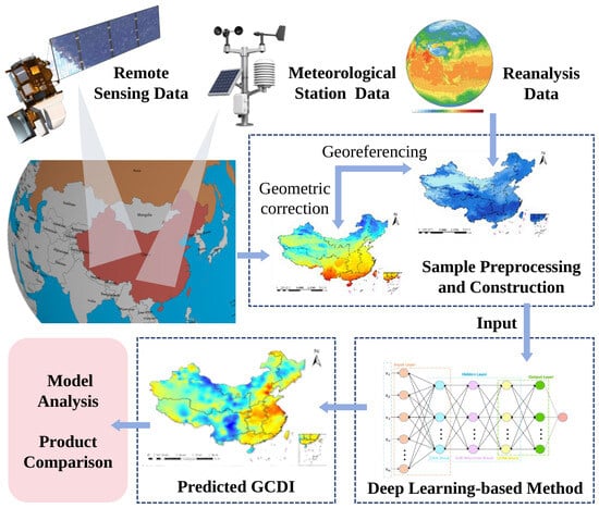
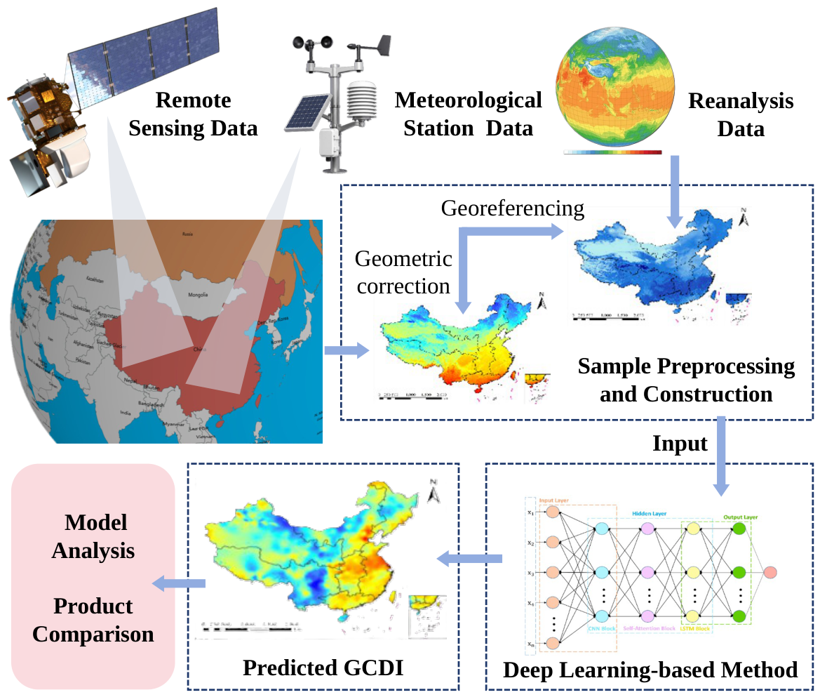
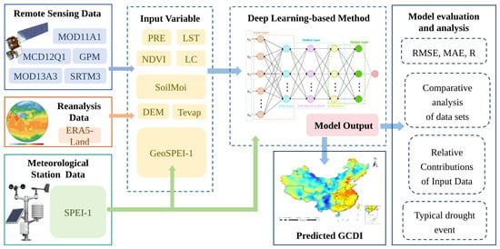
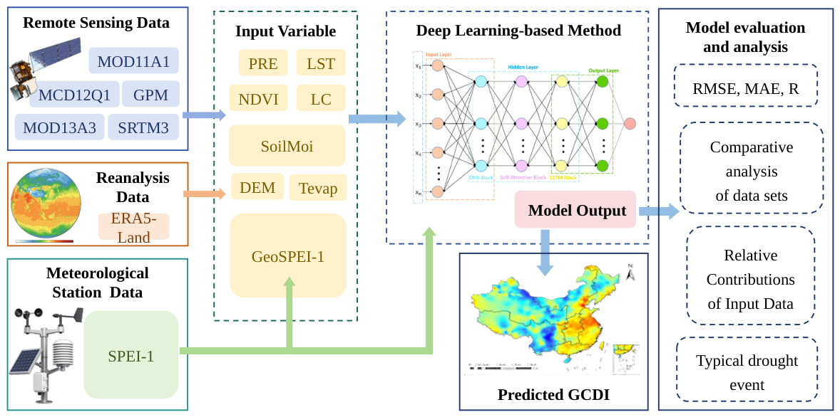
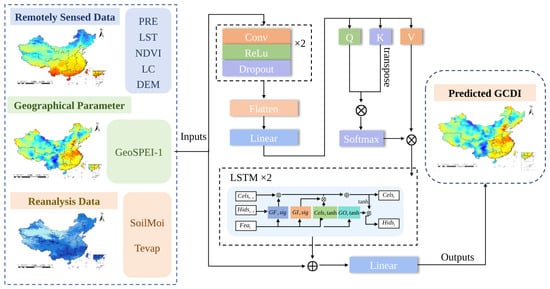
To address these limitations, this study develops a multi-source geo-aware feature learning framework to generate a monthly Geographically Weighted Composite Drought Index, termed GCDI-1, on a 1-km grid over China. The overall workflow of GCDI-1 generation is illustrated in Figure 1. The main contributions of this study are summarized as follows.

Figure 1. Overall workflow of drought product generation. Arrows indicate the flow of information between processing stages. Ellipses in the neural-network schematic denote omitted repeated units. Colored elements distinguish data sources and processing components; inset maps illustrate spatial input and output patterns.

1.

We construct a geographically weighted SPEI-related auxiliary variable, termed GeoSPEI-1, from neighboring station-based SPEI-1 values. GeoSPEI-1 incorporates neighboring-station drought information according to geographic distance and provides spatial auxiliary information for drought index generation.

2.

Based on GeoSPEI-1, we construct a deep learning model, termed GeoCSL, to jointly process GeoSPEI-1, remote sensing data, and reanalysis variables for drought index generation. GeoCSL combines convolutional neural network, self-attention, and long short-term memory components to process and integrate the multi-source input variables.

3.

We generate a monthly spatially continuous GCDI-1 product on a 1-km grid over China. During the temporally held-out 2011-2012 evaluation period, GCDI-1 achieved a station-referenced RMSE of 0.556 and MAE of 0.410, compared with 0.562 and 0.421 for leave-one-station-out Kriging and 0.754 and 0.577 for SPEIbase-1, respectively.

The remainder of this paper is organized as follows. Section 2 introduces the study area and datasets. Section 3 describes the proposed methodology. Section 4 presents the experimental design and analysis. Section 5 discusses the findings and limitations of GCDI-1. Finally, Section 6 summarizes this study.

2. Study Area and Data

2.1. Study Area

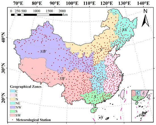
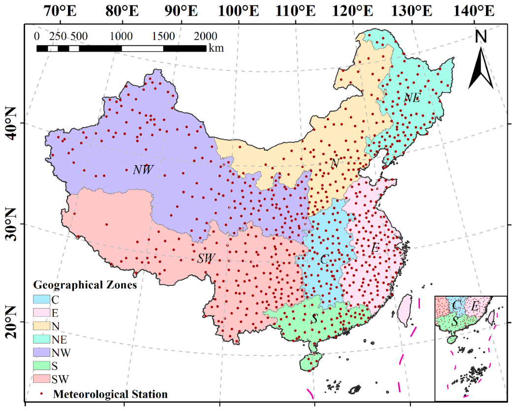
China was selected as the study area, and its geographic extent is shown in Figure 2. China covers approximately 9.6 million ${\mathrm{km}}^2$ and extends from $3°$ to $54°$N and from $73°$ to $135°$E. The country exhibits pronounced spatial heterogeneity in topography and climate, with generally higher terrain in the west and lower terrain in the east, and climatic conditions ranging from arid northwestern regions to humid southeastern regions. For regional description, China was divided into seven regions: eastern, central, northern, northeastern, northwestern, southwestern, and southern China.

Figure 2. Study area with geographical distribution of 804 meteorological stations. C, E, N, NE, NW, S, and SW denote central, eastern, northern, northeastern, northwestern, southern, and southwestern China, respectively.

2.2. Data Sources

To generate spatially continuous drought information across China, this study integrated meteorological station observations, satellite remote sensing (RS) products, reanalysis variables, and an existing gridded drought index product. These datasets were selected to represent meteorological, vegetation, hydrological, and topographic factors related to drought conditions. Station-based SPEI-1 was used as the supervised reference for model training and evaluation, while the RS and reanalysis variables were used as auxiliary predictors for drought index generation. The spatial resolutions reported below refer to the native resolutions or grid spacings of the original products. All gridded variables were subsequently harmonized to a common 1-km grid for model input, as described in the data preprocessing section.

Meteorological station observations: Daily meteorological observations were processed to calculate station-based SPEI-1. The resulting station-level SPEI-1 values were used as the reference drought variable for model training and evaluation. The original meteorological records were obtained from the China Meteorological Data Service Center (http://data.cma.cn/ (accessed on 9 June 2023)). The primary dataset used in this study was the China Surface Climate Data Daily Value Dataset (V3.0), which contains long-term daily meteorological records beginning in 1951. The dataset includes meteorological variables related to the hydrological cycle and drought conditions, including air pressure, air temperature, precipitation, evaporation, relative humidity, wind speed and direction, sunshine duration, and ground temperature. These observations provide the basis for estimating potential evapotranspiration and calculating SPEI. Because station-based SPEI-1 calculation requires temporally continuous meteorological records, the station dataset was screened before sample construction. Stations with continuous missing records longer than six months were excluded. For an additional 54 stations requiring monthly data reconstruction, missing year–month records were inserted chronologically, and missing precipitation and temperature values were filled using within-station linear interpolation. Missing values in the calculated SPEI series were also interpolated separately within each station. This procedure is distinct from the six-neighbor weighting used to construct GeoSPEI-1. After quality control and screening, 804 meteorological stations across mainland China were retained. Their spatial distribution is shown in Figure 2.

Remote sensing data: Satellite RS products were used to characterize spatially distributed vegetation, surface thermal, precipitation, land-cover, and topographic conditions associated with drought. Three groups of satellite-derived datasets were included: Moderate Resolution Imaging Spectroradiometer (MODIS) products, Global Precipitation Measurement (GPM) precipitation data, and Shuttle Radar Topography Mission (SRTM) elevation data. The derived variables included normalized difference vegetation index (NDVI), land surface temperature (LST), land cover (LC), digital elevation model (DEM), and GPM-based precipitation.

MODIS data: MODIS products were used to characterize vegetation conditions, surface thermal status, and land-cover types. LST was derived from the MOD11A1 product, which provides daily observations at a native spatial resolution of 1 km. Because the target drought index was generated at the monthly scale, daily LST observations were aggregated into monthly mean values. LST was included to represent surface thermal conditions related to evapotranspiration, soil moisture depletion, and vegetation water stress. Monthly NDVI was obtained from the MOD13A3 product at a native spatial resolution of 1 km and was used to characterize vegetation conditions and drought-related vegetation responses. In addition, the MCD12Q1 land-cover product, with an annual temporal resolution and a native spatial resolution of 500 m, was used to describe spatial differences in land-surface types.

GPM data: Precipitation data were obtained from the Integrated Multi-satellite Retrievals for GPM (IMERG) product of the Global Precipitation Measurement mission. The dataset used in this study provides monthly precipitation on a native $0.1°$ grid. Because precipitation represents the primary moisture input associated with meteorological drought and directly contributes to the climatic water balance underlying SPEI, GPM precipitation was included as an environmental predictor for GCDI-1 generation.

SRTM data: Topographic information was obtained from the SRTM V3 elevation product, which has a native spatial resolution of approximately 30 m. The resulting DEM was used to represent topographic differences that may be associated with spatial variations in precipitation, temperature, and evapotranspiration, thereby providing additional terrain information for drought index generation.

Reanalysis data: ERA5-Land reanalysis data were used to provide spatially continuous information on land-surface hydrothermal conditions. ERA5-Land is a global land-surface reanalysis dataset developed by the European Centre for Medium-Range Weather Forecasts (ECMWF) and provides long-term variables with high temporal continuity. In this study, soil moisture (SoilMoi) and total evapotranspiration (Tevap) were used as model predictors, while 2-m air temperature (T2) was used during data preprocessing to fill missing LST values. These ERA5-Land variables have a native grid spacing of approximately $0.1°$ and an hourly temporal resolution. Soil moisture was used to characterize land-surface water availability, while total evapotranspiration was used to represent water loss from the land surface and vegetation canopy.

Comparison drought product: SPEIbase v2.9 was used as an existing gridded SPEI product for comparison with GCDI-1. SPEIbase v2.9 provides global gridded SPEI at multiple accumulation timescales. It is generated from monthly precipitation and potential evapotranspiration, with potential evapotranspiration estimated using the Penman-Monteith method. The dataset provides SPEI series at timescales ranging from 1 to 48 months. In this study, the one-month SPEI product from SPEIbase v2.9 was used for comparison with GCDI-1 under the adopted station-referenced evaluation setting. SPEIbase v2.9 is provided on a $0.5°$ grid and therefore represents drought conditions at a substantially coarser grid scale than the 1-km output grid adopted for GCDI-1.

2.3. Calculation of Station-Based SPEI-1

Station-based SPEI-1 was calculated from meteorological station observations and used as the reference drought variable for model training and evaluation. SPEI extends the Standardized Precipitation Index (SPI) by incorporating potential evapotranspiration into the climatic water balance. Unlike SPI, which characterizes drought solely on the basis of precipitation variability, SPEI considers the difference between precipitation and potential evapotranspiration and therefore reflects the combined effects of water supply and atmospheric evaporative demand [18]. This formulation makes SPEI suitable for characterizing drought conditions under varying temperature and hydrothermal conditions.

Daily meteorological observations, including precipitation, mean 10-m wind speed, maximum and minimum air temperature, mean relative humidity, and sunshine duration, together with station latitude and elevation, were used to estimate potential evapotranspiration and construct the climatic water balance series. Specifically, reference evapotranspiration was estimated using the FAO Penman-Monteith method [51]. The daily reference evapotranspiration values were then aggregated to the monthly scale to obtain monthly potential evapotranspiration. Monthly precipitation and potential evapotranspiration were used to calculate the monthly climatic water balance. The accumulated water balance series was fitted using a three-parameter log-logistic distribution, with the distribution parameters estimated using L-moments. The corresponding cumulative probabilities were then standardized to obtain SPEI values [18]. The fitting period was determined according to the available long-term meteorological record at each station, generally spanning 1982–2017. The available record at each station was used to fit the three-parameter log-logistic distribution and calculate station-based SPEI-1. Based on the resulting SPEI values, drought conditions were classified into different severity levels according to commonly used SPEI classification criteria, as shown in Table 1.

Table 1. SPEI Drought Classification.

Level	SPEI	Types
1	$\mathrm{SPEI}>-0.5$	No drought
2	$-1.0<\mathrm{SPEI}\le -0.5$	Mild drought
3	$-1.5<\mathrm{SPEI}\le -1.0$	Moderate drought
4	$-2.0<\mathrm{SPEI}\le -1.5$	Severe drought
5	$\mathrm{SPEI}\le -2.0$	Extreme drought

For different SPEI timescales, the monthly climatic water balance series can be accumulated over corresponding time windows, such as 1, 3, 6, 9, and 12 months. In this study, one-month SPEI (SPEI-1) was selected to characterize short-term meteorological drought conditions because it is sensitive to monthly variations in precipitation and potential evapotranspiration.

2.4. Sample Preprocessing and Construction

Data preprocessing was conducted to ensure consistency among meteorological station observations, RS products, reanalysis variables, and auxiliary geographic data. Table 2 summarizes the datasets and their corresponding abbreviations. The spatial scales reported in Table 2 refer to the native spatial resolutions or grid spacings of the original datasets. Because these datasets differed in spatial resolution, temporal resolution, coordinate system, and data format, preprocessing was performed before sample construction. According to the data characteristics, the preprocessing procedure consisted of two parts: meteorological station data processing and gridded auxiliary data processing.

Table 2. Data abbreviations of variables.

Abbreviation	Data	Native Spatial Resolution/Grid Spacing	Temporal Resolution
SPEI-1	SPEI at a monthly scale	–	1 month
LST	Land surface temperature	1000 m	1 day
PRE	Precipitation	$0.1°$	1 month
NDVI	Normalized difference vegetation index	1000 m	1 month
DEM	Digital elevation model	30 m	–
LC	Land cover type	500 m	1 year
SoilMoi	Soil moisture	$0.1°$	1 h
Tevap	Total evapotranspiration	$0.1°$	1 h
T2	2-m air temperature (for LST gap filling)	$0.1°$	1 h

For the meteorological station data, station-based SPEI-1 values calculated using the method described in Section 2.3 were used as the supervised target for sample construction. Each station-based SPEI-1 value was matched with the corresponding RS, reanalysis, and auxiliary geographic variables according to station location and month, thereby generating station-month samples for model development and evaluation.

The RS and reanalysis datasets were preprocessed using the Google Earth Engine platform. The preprocessing steps included unifying the geographic coordinate system to GCS_WGS_1984, harmonizing the temporal scale, and clipping all datasets to the study area using the boundary of China. Because the original datasets have different native spatial resolutions or grid spacings, all gridded variables were subsequently resampled to a common 1000 m × 1000 m grid using the nearest-neighbor method to ensure spatial alignment among the model inputs. This common grid was used for subsequent variable matching and GCDI-1 generation. It should be emphasized that the resampling procedure only harmonizes the grid spacing and spatial alignment of the input datasets and does not increase the intrinsic spatial information content of datasets originally available at coarser spatial scales, such as GPM and ERA5-Land.

After spatial and temporal harmonization, point-to-pixel matching was performed according to the geographic coordinates of each meteorological station. The values of the corresponding gridded auxiliary variables were extracted from the grid cell containing each station and matched with the station-based SPEI-1 value for the same month. In this way, station-month samples were constructed by pairing each station-based SPEI-1 value with the corresponding LST, PRE, SoilMoi, NDVI, DEM, Tevap, and LC values for the same station location and month. Samples containing unresolved missing or abnormal gridded values were removed during data preprocessing. Because the LST dataset contained relatively extensive missing areas, ERA5-Land 2-m air temperature was used to fill missing LST values after confirming a high correlation between the two variables. Before model training, the input predictor variables were standardized column-wise using StandardScaler. The station-based SPEI-1 values used as the supervised target were not standardized.

Finally, a total of 164,016 matched station-month samples containing SPEI-1 values and all input variables were obtained for the period from 2001 to 2017. Among them, 96,480 samples from 2001 to 2010 were used for model training, while 19,296 samples from 2011 to 2012 were reserved as the temporally held-out test set. The remaining 48,240 samples from 2013 to 2017 were used for an additional temporal evaluation, product mapping, and drought-event analysis.

3. Methodology

The overall drought index generation framework is shown in Figure 3. The framework integrates meteorological station information, multi-source RS data, and reanalysis variables to generate the Geographically Weighted Composite Drought Index (GCDI-1). Station-based SPEI-1 is used as the supervised reference variable. To incorporate neighboring-station drought information into the generation process, a geographically weighted SPEI-related auxiliary variable, termed GeoSPEI-1, is constructed from neighboring station-based SPEI-1 values. GeoSPEI-1 is jointly used with multi-source RS and reanalysis variables as input to GeoCSL. Here, “composite” refers to the integration of these information sources to generate GCDI-1. GeoCSL combines convolutional neural network (CNN), self-attention (SA), and long short-term memory (LSTM) components to process and integrate the multi-source input features. The trained model is subsequently applied to the spatially continuous gridded inputs to generate monthly GCDI-1 on a 1-km grid over China.

Figure 3. Workflow of the multi-source geo-aware feature-learning framework, including data preprocessing, GeoSPEI-1 construction, GeoCSL modeling, and GCDI-1 generation.

3.1. Geographically Weighted SPEI-1 Auxiliary Variable

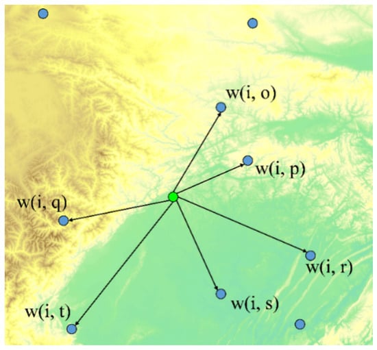
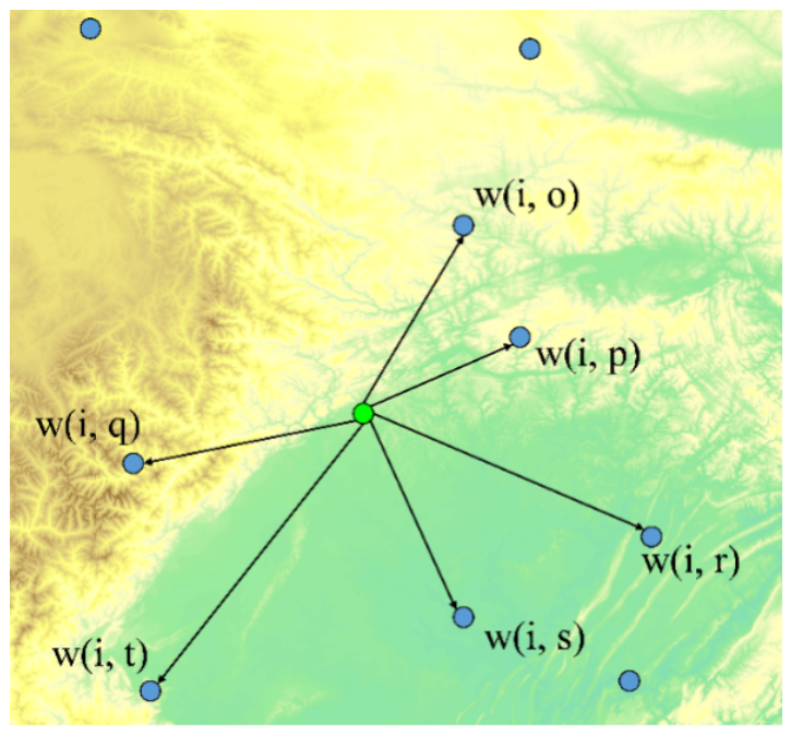
To incorporate neighboring-station drought information into GCDI-1 generation, this study constructs a geographically weighted SPEI-related auxiliary variable, termed GeoSPEI-1. GeoSPEI-1 is not treated as an independent drought index; instead, it provides geographically weighted information derived from neighboring station-based SPEI-1 observations. For each target location and month, six neighboring meteorological stations were used to construct GeoSPEI-1. For station-based samples used for model training and evaluation, the target station itself was first excluded from the candidate station set, after which the six nearest neighboring stations were selected. For ordinary grid cells used for spatial GCDI-1 generation, the six nearest available meteorological stations were directly selected. The SPEI-1 values of the selected neighboring stations for the same month were then combined using Gaussian distance weights, as illustrated in Figure 4.

Figure 4. Schematic illustration of GeoSPEI-1 construction from neighboring meteorological stations. Blue circles indicate neighboring meteorological stations, and the green circle denotes the target location. Connecting lines indicate station-to-target geographical weighting relationships.

The Gaussian distance weights assign larger contributions to stations closer to the target location and smaller contributions to more distant stations. GeoSPEI-1 is calculated as follows:

$$\mathrm{GeoSPEI}-1_{s,t}={\displaystyle \frac{{\sum }_{i=1}^n{w}_{s,i}\mathrm{SPEI}-1_{i,t}}{{\sum }_{i=1}^n{w}_{s,i}}},$$

(1)

where n denotes the number of neighboring meteorological stations ($n=6$ in this study), $\mathrm{SPEI}-1_{i,t}$ denotes the station-based SPEI-1 value of the i-th neighboring station at month t, and $w_{s,i}$ denotes the geographical weight between target location s and the i-th neighboring station. The geographical weight is determined using a Gaussian distance-weighting function:

$$w_{s,i}=\exp \left(-{\displaystyle \frac{d_{s,i}^2}{2{\sigma }_s^2}}\right),$$

(2)

$${\sigma }_s={\displaystyle \frac{1}{2}}\left({\displaystyle \frac{1}{n}}{\displaystyle \sum _{i=1}^n}{d}_{s,i}\right),n=6,$$

(3)

where $d_{s,i}$ denotes the geographic distance between target location s and the i-th neighboring station. Rather than using a single fixed bandwidth for all locations, ${\sigma }_s$ is determined adaptively as one-half of the mean distance from the target location to its six nearest neighboring stations. Therefore, the Gaussian distance-decay scale varies according to the local spacing of the meteorological station network. In addition, the geographic distance is calculated using the Vincenty method:

$$d_{s,i}=\mathrm{Vincenty}\left[(Lon,Lat),(Lo{n}_i,La{t}_i)\right],$$

(4)

where $(Lon,Lat)$ denotes the longitude and latitude of target location s, and $(Lo{n}_i,La{t}_i)$ denotes the longitude and latitude of the i-th neighboring meteorological station.Through this geographically weighted calculation, GeoSPEI-1 incorporates neighboring station-based SPEI-1 information according to geographic distance and is subsequently used together with the multi-source RS and reanalysis variables as input to GeoCSL for GCDI-1 generation.

3.2. Geographically Weighted CNN-SA-LSTM Network

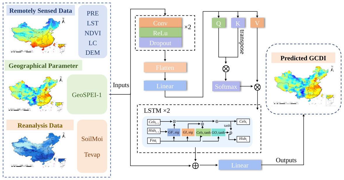
To jointly process GeoSPEI-1 and the multi-source environmental variables, this study constructs a geographically weighted CNN-SA-LSTM model, termed GeoCSL, for GCDI-1 generation. As shown in Figure 5, GeoCSL sequentially combines CNN blocks, an SA module, and LSTM blocks to process the input features.

Figure 5. Architecture of GeoCSL, consisting of CNN blocks, a self-attention (SA) module, and LSTM blocks. Arrows indicate feature flow and the residual connection. Dashed boxes group the input data sources and network components. Colors distinguish feature groups, operations, and attention/gating elements rather than numerical magnitudes. The notation $\times 2$ denotes repeated blocks.

For a grid cell s in month t, the input feature vector of GeoCSL is defined as ${\mathbf{X}}_{s,t}$:

$${\mathbf{X}}_{s,t}=[{\mathrm{PRE}}_{s,t},{\mathrm{LST}}_{s,t},{\mathrm{Tevap}}_{s,t},{\mathrm{SoilMoi}}_{s,t},{\mathrm{NDVI}}_{s,t},{\mathrm{DEM}}_s,{\mathrm{LC}}_s,\mathrm{GeoSPEI}-1_{s,t}].$$

(5)

The station-based SPEI-1 value is used as the supervised target, i.e., $Y_{s,t}=\mathrm{SPEI}-1_{s,t}$, and the overall generation function of GeoCSL can be expressed as

$$\mathrm{GCDI}-1_{s,t}=\mathrm{GeoCSL}\left({\mathbf{X}}_{s,t}\right),$$

(6)

where $PRE$, $LST$, and $Tevap$ represent precipitation, land surface temperature, and total evapotranspiration, respectively; $SoilMoi$ and $NDVI$ denote soil moisture and vegetation condition; $DEM$ and $LC$ represent terrain and land-cover information, respectively; and $\mathrm{GeoSPEI}-1_{s,t}$ denotes the geographically weighted SPEI-related auxiliary variable constructed from neighboring station-based SPEI-1 values. $\mathrm{GeoCSL}(·)$ denotes the GeoCSL model, and $\mathrm{GCDI}-1_{s,t}$ denotes the generated GCDI-1 value at grid cell s in month t. Each sample corresponds to a single target month. In the implemented GeoCSL model, the temporal input length is $T=1$; therefore, no multi-month sequence is provided within an individual sample.

Feature Extraction: The eight input variables are first processed using two one-dimensional CNN blocks. The CNN input feature size is 8, with hidden feature dimensions of 128 and 256 and an output feature dimension of 8. The convolution kernel size is 3, the padding size is 1, and a dropout rate of 0.2 is used. The resulting feature maps are then flattened and projected through a fully connected layer to obtain the feature representation used by the subsequent SA module.

Feature Dependency Modeling: An SA module is applied to the CNN-derived representation to model dependencies among the learned drought-related features. The feature dimension of the SA module is 8. The attention-enhanced representation is then passed to the subsequent LSTM module.

LSTM-based Feature Transformation: The attention-enhanced feature representation is further processed by a two-layer LSTM module. The LSTM input feature dimension is 8, the hidden dimension is 64, and the number of stacked layers is 2. In the implementation used in this study, each sample contains only one target month and the sequence length is $T=1$. Therefore, the LSTM does not incorporate observations from preceding months within an individual sample and is not interpreted here as explicitly modeling multi-month temporal evolution. The 64-dimensional LSTM hidden representation is projected to eight dimensions and added element-wise to the original standardized input features through a residual connection. The resulting features are then passed through a fully connected layer to generate GCDI-1.

During model training, station-based SPEI-1 is used as the supervised target, and the GeoCSL model is optimized using the L1 loss. After training and validation, the optimized GeoCSL model is applied to spatially continuous gridded input variables to generate monthly GCDI-1 maps on a 1-km grid over China.

4. Experiments and Analysis

4.1. Experimental Settings

From 2001 to 2017, a total of 164,016 matched station-month samples were obtained, each containing a station-based SPEI-1 value and the corresponding input variables. The samples were divided according to year. Specifically, 96,480 samples from 2001 to 2010 were used for model training, while 19,296 samples from 2011 to 2012 were reserved as the temporally held-out test set. The same meteorological station network was represented in both periods; therefore, the 2011–2012 test set evaluates temporal generalization at existing station locations rather than spatial transferability to previously unseen stations or regions. The remaining 48,240 samples from 2013 to 2017 were used for an additional temporal evaluation, product mapping, and drought-event analysis.

Ten-fold cross-validation was conducted using only the 2001–2010 training samples for hyperparameter selection and internal model validation [52,53]. Neither the temporally held-out test samples from 2011 to 2012 nor the samples from 2013 to 2017 were involved in this procedure. Specifically, the samples from 2001 to 2010 were randomly divided into ten subsets. In each run, one subset was used for validation and the remaining nine subsets were used for model training. This procedure was repeated ten times so that each subset was used once for validation.

To evaluate GeoCSL and examine the contribution of GeoSPEI-1, three comparison models were considered: CSL, DFNN [54], and RF [47]. CSL has the same network structure as GeoCSL but does not include GeoSPEI-1 as an input variable. DFNN and RF were also implemented using the same multi-source environmental variables without GeoSPEI-1. For RF, the ensemble consisted of 100 decision trees, with the maximum tree depth set to 14. The minimum numbers of samples required to split an internal node and to form a leaf node were set to 4 and 2, respectively. At each split, the candidate feature subset was selected using the square-root strategy, and bootstrap sampling was adopted. For the deep-learning models, training was conducted for a maximum of 300 epochs with a learning rate of 0.001 and a batch size of 64. GeoCSL was optimized using the Adam optimizer with L1 loss. An early-stopping strategy was applied based on the mean training MAE loss of each epoch. Training was terminated if the mean training loss did not improve for 10 consecutive epochs, with 300 epochs as the maximum training duration. Neither the validation data nor the temporally held-out test data were used to determine the stopping point. A fixed random seed of 42 was used.

Before model training, the input predictor variables were standardized column-wise using StandardScaler, with the scaling parameters estimated from the 2001–2010 training data. The station-based SPEI-1 values used as the supervised target were not standardized. To further examine whether the contribution of GeoSPEI-1 is consistent across different model types, additional paired experiments were conducted using RF and DFNN. For each model, two input settings were compared: M + S + T without GeoSPEI-1 and G + M + S + T with GeoSPEI-1. Within each model pair, the same ten-fold partitions and hyperparameter settings were used, with a fixed random seed of 42.

To evaluate model performance, three primary metrics were adopted: Root Mean Squared Error ($RMSE$), Mean Absolute Error ($MAE$), and Pearson correlation coefficient (R). In addition, Positive Mean Error ($PME$) and Negative Mean Error ($NME$) were used in the station-referenced product comparison to characterize the magnitudes of positive and negative index-value errors.

$RMSE$ measures the overall deviation between the generated drought index and station-based SPEI-1 and gives greater weight to relatively large errors. It is defined as Equation (7):

$$RMSE=\sqrt{{\displaystyle \frac{1}{N}}\sum _{i=1}^N{\left({\widehat{y}}_i-y_i\right)}^2}$$

(7)

$MAE$ measures the average absolute difference between the generated drought index and station-based SPEI-1. Compared with $RMSE$, it is less sensitive to relatively large errors and provides a direct measure of the average absolute estimation error. It is defined as Equation (8):

$$MAE={\displaystyle \frac{1}{N}}{\displaystyle \sum _{i=1}^N}\left|{\widehat{y}}_i-y_i\right|$$

(8)

The Pearson correlation coefficient (R) was used to quantify the strength and direction of the linear association between the generated drought index and station-based SPEI-1. It is defined as

$$R={\displaystyle \frac{{\sum }_{i=1}^N({\widehat{y}}_i-\overline{\widehat{y}})(y_i-\overline{y})}{\sqrt{{\sum }_{i=1}^N{({\widehat{y}}_i-\overline{\widehat{y}})}^2{\sum }_{i=1}^N{(y_i-\overline{y})}^2}}},$$

(9)

The value of R ranges from $-1$ to 1. Values closer to 1 indicate a stronger positive linear association, values closer to $-1$ indicate a stronger negative linear association, and values closer to 0 indicate a weaker linear association.

$PME$ represents the mean positive index-value error for samples satisfying ${\widehat{y}}_i-y_i>0$ and is defined as Equation (10):

$$PME={\displaystyle \frac{1}{N_{+}}}\sum _{{\widehat{y}}_i-y_i>0}\left({\widehat{y}}_i-y_i\right)$$

(10)

A larger $PME$ indicates a larger mean positive deviation between the generated drought index and station-based SPEI-1.

$NME$ represents the mean negative index-value error for samples satisfying ${\widehat{y}}_i-y_i<0$ and is defined as Equation (11):

$$NME={\displaystyle \frac{1}{N_{-}}}\sum _{{\widehat{y}}_i-y_i<0}\left({\widehat{y}}_i-y_i\right)$$

(11)

Because $NME$ is calculated from negative errors, its value is negative, and a larger absolute value of $NME$ indicates a larger mean negative deviation.

Here, $y_i$ denotes the station-based SPEI-1 value, ${\widehat{y}}_i$ denotes the corresponding generated drought-index value, N denotes the total number of samples, $\overline{y}$ and $\overline{\widehat{y}}$ denote the mean station-based SPEI-1 value and mean generated drought-index value, respectively, and $N_{+}$ and $N_{-}$ denote the numbers of samples satisfying ${\widehat{y}}_i-y_i>0$ and ${\widehat{y}}_i-y_i<0$, respectively.

4.2. Effects of Auxiliary Variable Combinations

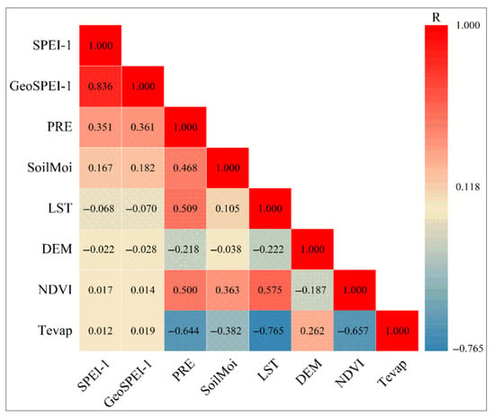
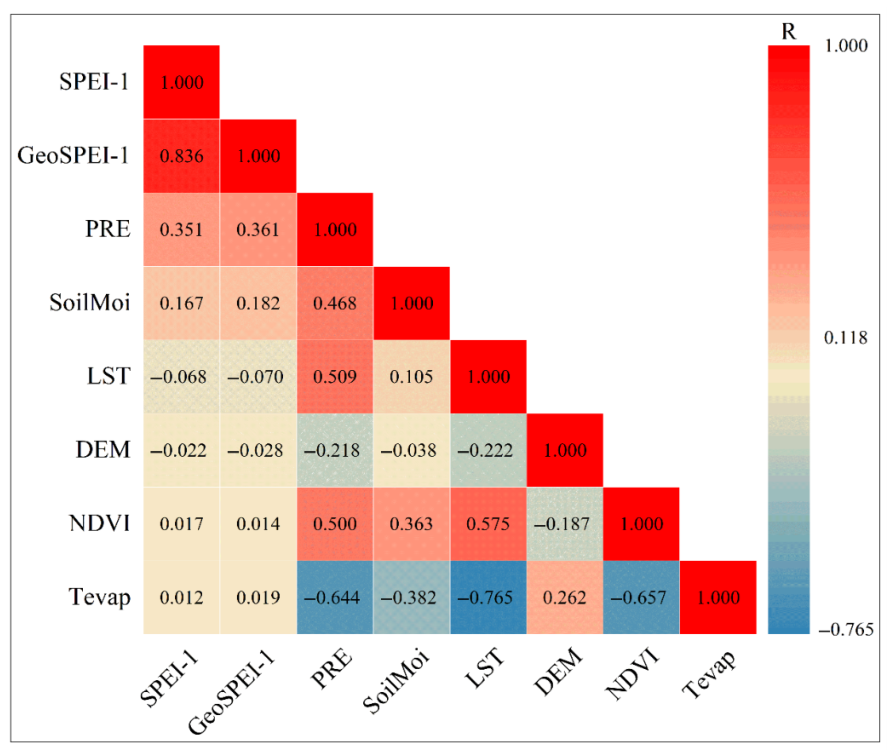
The linear associations between the input variables and station-based SPEI-1 were evaluated using Pearson correlation coefficients. Figure 6 presents the Pearson correlation coefficient (R) between each input variable and station-based SPEI-1. Among the input variables, GeoSPEI-1 showed the strongest linear association with station-based SPEI-1, with an R value greater than 0.8. PRE and SoilMoi showed moderate linear associations with station-based SPEI-1, whereas LST, NDVI, DEM, and Tevap showed relatively weaker associations. These results indicate that GeoSPEI-1 contains information that is strongly associated with station-based SPEI-1, while the individual environmental variables exhibit different degrees of linear association with station-based SPEI-1.

Figure 6. Pearson correlation coefficients between input variables and station-based SPEI-1.

To examine the effects of different input-variable combinations on GeoCSL performance, different combinations of the input variables were evaluated using the same GeoCSL architecture, as summarized in Table 3. When only the environmental variable groups M, S, and T were used, GeoCSL obtained an $RMSE$ of 0.735, an $MAE$ of 0.572, and an R of 0.708. When GeoSPEI-1 was used as the sole input to GeoCSL (G), the corresponding $RMSE$, $MAE$, and R were 0.578, 0.426, and 0.812, respectively. The substantial difference between M + S + T and G indicates that geographically weighted neighboring-station information provides the dominant information source among the evaluated input groups.

Table 3. Model performance under different combinations of input variables based on ten-fold cross-validation using the 2001–2010 training samples.

Input Combination	RMSE	MAE	R
M + S + T	0.735	0.572	0.708
G	0.578	0.426	0.812
G + S	0.563	0.418	0.841
G + T	0.564	0.418	0.841
G + M	0.553	0.411	0.847
G + S + T	0.562	0.417	0.842
G + M + S	0.551	0.409	0.849
G + M + T	0.550	0.409	0.850
G + M + S + T	0.546	0.407	0.851

Note: M represents meteorological variables (LST, PRE, and Tevap); S represents land-surface condition variables (SoilMoi and NDVI); T represents geographic variables (DEM and LC); and G represents GeoSPEI-1 used as the sole input to GeoCSL.

When the environmental variable groups were combined with GeoSPEI-1, GeoCSL performance generally improved. Among the combinations obtained by adding one environmental variable group to GeoSPEI-1, G + M achieved an $RMSE$ of 0.553, an $MAE$ of 0.411, and an R of 0.847, while G + S and G + T produced smaller improvements. The best performance was obtained when all four variable groups were jointly used (G + M + S + T), with an $RMSE$ of 0.546, an $MAE$ of 0.407, and an R of 0.851. These results indicate that GeoSPEI-1 provides the primary information source for GeoCSL, while the multi-source environmental variables provide additional complementary information for GCDI-1 generation. The relative contributions of these input data groups were assessed through their effects on GeoCSL performance, corresponding to the analysis illustrated in Figure 3.

4.3. Model Performance

The overall performance of GeoCSL and the comparison models was evaluated using ten-fold cross-validation on the 2001–2010 training samples, as described in Section 4.1. Figure 7 presents the scatter plots of the estimated drought-index values against station-based SPEI-1 for DFNN [54], RF [47], CSL, and GeoCSL.

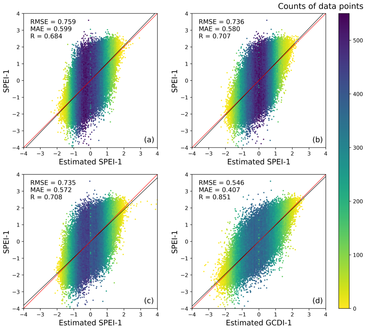
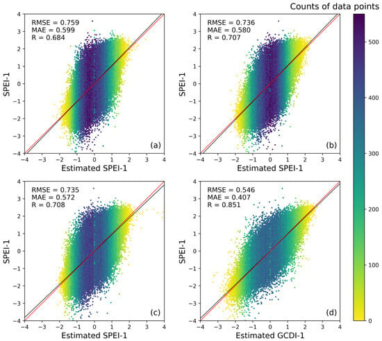
Figure 7. Scatter plots of out-of-fold predictions against station-based SPEI-1 for (a) DFNN, (b) RF, (c) CSL, and (d) GeoCSL based on ten-fold cross-validation using the 2001–2010 training samples.

As shown in Figure 7, the fitted lines for the four models show different degrees of agreement with the 1:1 line. DFNN obtained an $RMSE$ of 0.759, an $MAE$ of 0.599, and an R of 0.684. Its estimated values were more concentrated around the central range, with larger dispersion toward the extremes. RF achieved an $RMSE$ of 0.736, an $MAE$ of 0.580, and an R of 0.707. CSL obtained an $RMSE$ of 0.735, an $MAE$ of 0.572, and an R of 0.708. GeoCSL, which additionally incorporates GeoSPEI-1, achieved the best overall performance among the four models, with an $RMSE$ of 0.546, an $MAE$ of 0.407, and an R of 0.851. Compared with CSL, which uses the same network architecture without GeoSPEI-1, the improved performance further indicates the important contribution of geographically weighted neighboring-station information to GeoCSL. Overall, these results are consistent with the input-combination experiments in Section 4.2, indicating that GeoSPEI-1 provides an important source of information for GeoCSL, while the multi-source environmental variables provide additional complementary information.

To further examine whether the contribution of GeoSPEI-1 is consistent across different model types, GeoSPEI-1 was additionally introduced into RF and DFNN, and the corresponding results were compared with the CSL-GeoCSL pair. As shown in Table 4, CSL achieved an $RMSE$ of 0.735, an $MAE$ of 0.572, and an R of 0.708 without GeoSPEI-1, whereas GeoCSL achieved 0.546, 0.407, and 0.851, respectively, after incorporating GeoSPEI-1. For RF, the corresponding metrics changed from 0.736, 0.580, and 0.707 to 0.552, 0.412, and 0.848 after GeoSPEI-1 was introduced. Similarly, DFNN achieved an $RMSE$ of 0.759, an $MAE$ of 0.599, and an R of 0.684 without GeoSPEI-1, compared with 0.554, 0.418, and 0.847, respectively, with GeoSPEI-1. The consistent improvement observed for CSL, RF, and DFNN indicates that the contribution of geographically weighted neighboring-station information is not restricted to a specific model architecture. These results further support GeoSPEI-1 as an important information source across the evaluated models.

Table 4. Performance of different models with and without GeoSPEI-1 based on ten-fold cross-validation using the 2001–2010 training samples.

Model	Input	RMSE	MAE	R
RF	M + S + T	0.736	0.580	0.707
RF + GeoSPEI-1	G + M + S + T	0.552	0.412	0.848
DFNN	M + S + T	0.759	0.599	0.684
DFNN + GeoSPEI-1	G + M + S + T	0.554	0.418	0.847
CSL	M + S + T	0.735	0.572	0.708
GeoCSL	G + M + S + T	0.546	0.407	0.851

4.4. Ablation Analysis of GeoCSL Components

To further examine the contribution of the network components in GeoCSL, an ablation experiment was conducted by evaluating different combinations of CNN, self-attention (SA), and LSTM components under the same experimental setting. Five configurations were considered: CNN, LSTM, CNN + SA, CNN + LSTM, and CNN + SA + LSTM. The results are summarized in Table 5.

Table 5. Ablation results for different component configurations of GeoCSL based on ten-fold cross-validation using the 2001–2010 training samples.

Configuration	RMSE	MAE	R
CNN	0.550	0.411	0.848
LSTM	0.556	0.414	0.845
CNN + SA	0.552	0.411	0.848
CNN + LSTM	0.550	0.412	0.849
CNN + SA + LSTM	0.546	0.407	0.851

Among the individual-component configurations, CNN achieved an $RMSE$ of 0.550, an $MAE$ of 0.411, and an R of 0.848, whereas LSTM obtained an $RMSE$ of 0.556, an $MAE$ of 0.414, and an R of 0.845. Adding SA to CNN resulted in an $RMSE$ of 0.552, an $MAE$ of 0.411, and an R of 0.848, while the CNN + LSTM configuration yielded an $RMSE$ of 0.550, an $MAE$ of 0.412, and an R of 0.849. These results show that adding an individual component did not consistently improve all evaluation metrics. The complete CNN + SA + LSTM configuration achieved the best overall performance among the five evaluated configurations, with an $RMSE$ of 0.546, an $MAE$ of 0.407, and an R of 0.851. Compared with CNN alone, the complete configuration reduced both $RMSE$ and $MAE$ while increasing R. It also outperformed the CNN + SA and CNN + LSTM configurations across all three metrics. These results indicate that the combination of CNN, SA, and LSTM provides better overall estimation performance than the evaluated individual or partial configurations. Under the single-month sample formulation adopted in this study, this ablation analysis is interpreted as an assessment of the contribution of the network components rather than evidence of multi-month temporal modeling capability.

4.5. Spatial and Temporal Evaluation of Model Performance

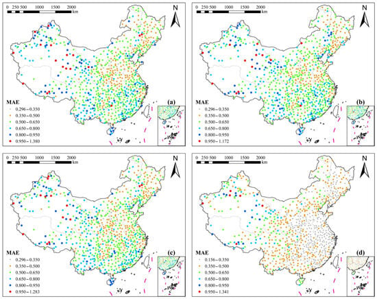
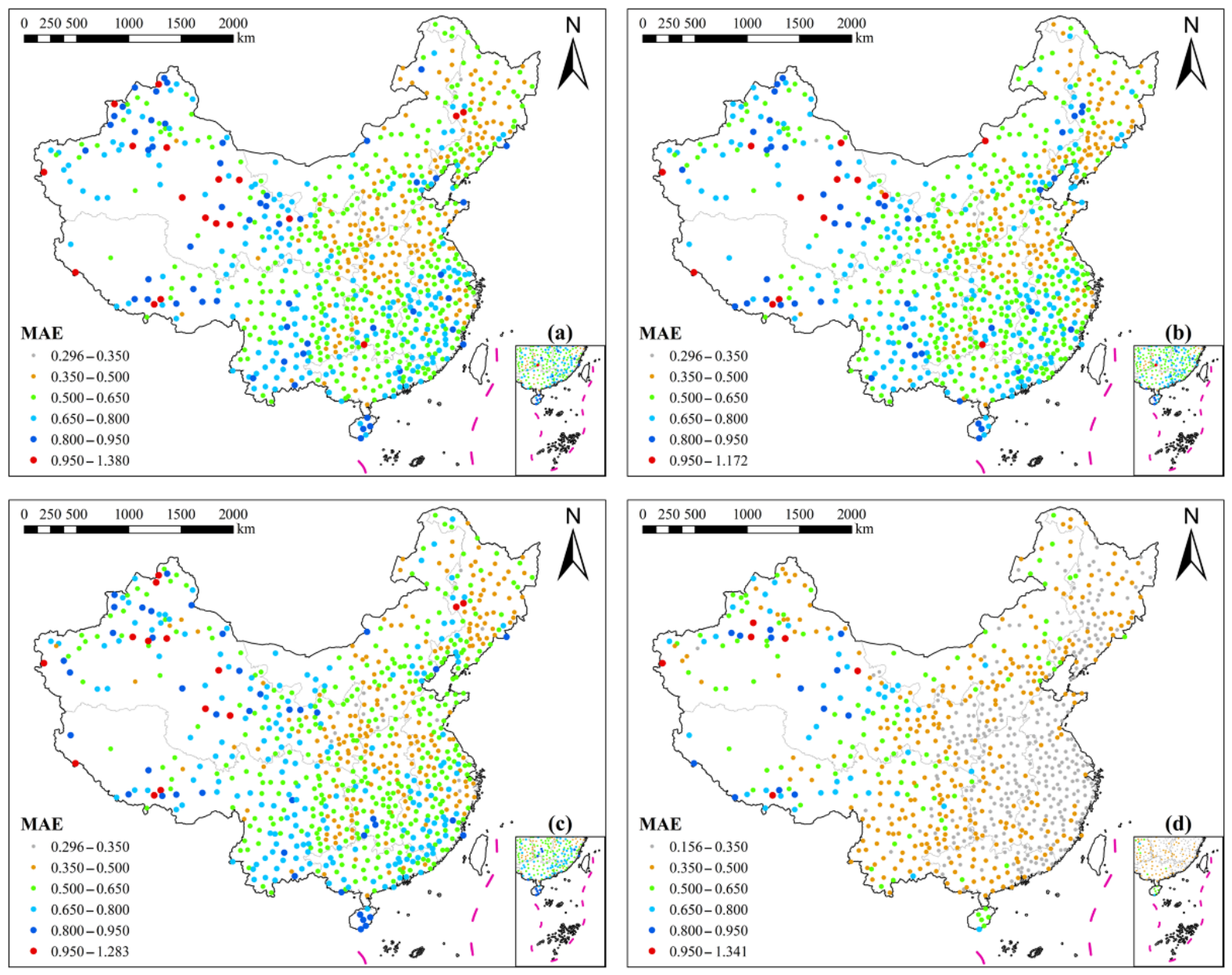
To examine the spatial variation in model performance, the $MAE$ was calculated for each meteorological station. Figure 8 presents the spatial distribution of station-level $MAE$ for the four models. For DFNN, the $MAE$ ranged from 0.296 to 1.380, with 263 stations showing $MAE$ values above 0.650, mainly distributed in southwestern, northwestern, and eastern China. For RF, the maximum $MAE$ decreased to 1.172, and 261 stations had $MAE$ values above 0.650, with many of these stations located in southwestern, northwestern, and southern China. For CSL, 239 stations had $MAE$ values above 0.650, while relatively lower errors were observed in northern, central, and eastern China. GeoCSL showed lower station-level errors overall, with only 62 stations having $MAE$ values above 0.650.

Figure 8. Spatial distribution of station-level $MAE$ for (a) DFNN, (b) RF, (c) CSL, and (d) GeoCSL during the temporally held-out 2011–2012 evaluation period.

The number of stations with $MAE$ values above 0.95 was 6 for GeoCSL, compared with 14, 13, and 18 for CSL, RF, and DFNN, respectively. The station-level $MAE$ of GeoCSL ranged from approximately 0.156 to 1.341, and most stations had $MAE$ values below 0.650. Compared with CSL, after GeoSPEI-1 was incorporated, the number of stations with $MAE$ values between 0.500 and 0.650 decreased by 236, while the numbers of stations with $MAE$ values between 0.350 and 0.500 and between 0 and 0.350 increased by 99 and 314, respectively. These results indicate an overall reduction in station-level estimation errors after the incorporation of GeoSPEI-1. Spatial differences nevertheless remained, with relatively higher errors occurring more frequently in northwestern and southwestern China.

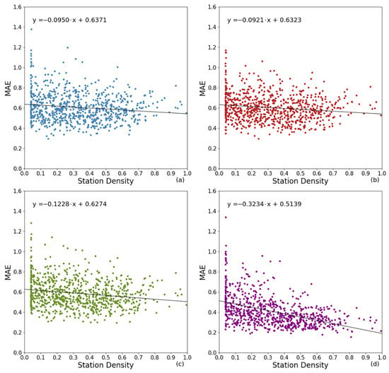
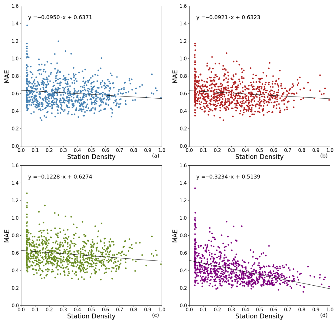
Because meteorological station density varies considerably across China, the relationship between station density and station-level $MAE$ was further examined. Station density was calculated using the Kernel Density tool in ArcGIS 10.8. As shown in Figure 9, station-level $MAE$ generally decreased with increasing station density across the four models, indicating an association between denser station distributions and lower estimation errors. Compared with the other models, GeoCSL showed a more pronounced decrease in station-level $MAE$ with increasing station density, suggesting a stronger dependence of its estimation performance on station density.

Figure 9. Relationship between station density and station-level $MAE$ for (a) DFNN, (b) RF, (c) CSL, and (d) GeoCSL during the temporally held-out 2011–2012 evaluation period.

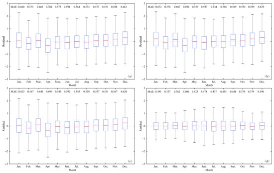
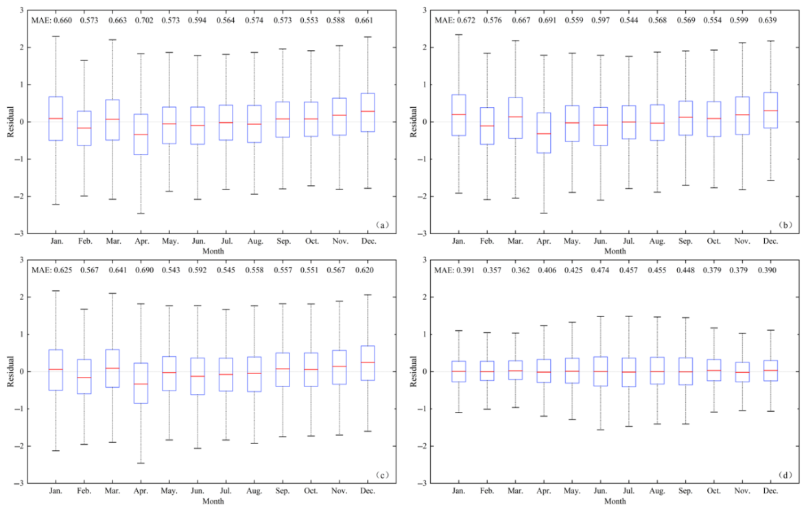
Model performance was also evaluated on a monthly scale using the temporally held-out test samples from 2011 to 2012. Figure 10 presents the distributions of monthly residuals, defined as the difference between the estimated and station-based SPEI-1 values. The median residuals of DFNN and RF varied across months and were below zero in February, April, June, and August, indicating a tendency to underestimate station-based SPEI-1 in these months. In comparison, the monthly median residuals of GeoCSL remained closer to zero. GeoCSL also showed a smaller spread in residuals than the comparison models, particularly in April, when DFNN and RF exhibited relatively large residual fluctuations.

Figure 10. Boxplots of month-specific residuals for (a) DFNN, (b) RF, (c) CSL, and (d) GeoCSL during the temporally held-out 2011–2012 evaluation period.

The monthly $MAE$ results further showed that model performance varied across months. GeoCSL achieved its lowest $MAE$ in February, with a value of 0.357, whereas higher $MAE$ values were observed from June to August. These results indicate that month-to-month variation in estimation error remained even after GeoSPEI-1 was incorporated.

To further evaluate model performance over a later period, an additional station-referenced evaluation was conducted using 48,240 station-month samples from 2013 to 2017. GeoCSL achieved an $RMSE$ of 0.593, an $MAE$ of 0.438, and an R of 0.840 during this period. These results provide an additional quantitative evaluation of the model over 2013–2017.

4.6. Comparative Product Evaluation

SPEIbase-1, Direct GeoSPEI-1, Kriging, and GCDI-1 were compared against station-based SPEI-1 during 2011–2012. SPEIbase-1 is a $0.5°$ gridded product, while Direct GeoSPEI-1 directly uses the geographically weighted average of six neighboring stations without GeoCSL. The target station was excluded when constructing Direct GeoSPEI-1. Kriging was evaluated using leave-one-station-out interpolation with an isotropic spherical variogram. Station coordinates were transformed into the China Albers projection, and empirical semivariances were calculated using the 2001–2010 station observations and grouped into 20 distance bins. The variogram parameters were fitted using PyKrige 1.7.3 with bounded soft-L1 optimization and short-distance logistic weighting. For each target station, variogram fitting and interpolation excluded that station, and the fitted parameters remained fixed across the 24 evaluation months. As shown in Table 6, GCDI-1 achieved an $RMSE$ of 0.556 and an $MAE$ of 0.410, compared with 0.572 and 0.421 for Direct GeoSPEI-1 and 0.562 and 0.421 for Kriging. These results indicate that the complete framework provides a modest additional improvement over directly using neighboring-station information.

Table 6. Station-referenced comparison of SPEIbase-1, Direct GeoSPEI-1, Kriging, and GCDI-1 during the 2011–2012 evaluation period. Kriging was evaluated using leave-one-station-out interpolation.

Method/Product	RMSE	MAE	PME	NME
SPEIbase-1	0.754	0.577	0.612	−0.527
Direct GeoSPEI-1	0.572	0.421	0.425	−0.418
Kriging	0.562	0.421	0.424	−0.418
GCDI-1	0.556	0.410	0.420	−0.400

To assess the small performance difference between GCDI-1 and Kriging, a paired station-cluster bootstrap was conducted using 19,296 station-month records from 804 stations. A total of 20,000 bootstrap replicates were performed by resampling stations with replacement while retaining their 24 monthly records. The $RMSE$ difference (Kriging minus GCDI-1) was 0.006781, with a 95% confidence interval of 0.001826–0.011869. The corresponding $MAE$ difference was 0.010527, with a 95% confidence interval of 0.006782–0.014357. Both intervals excluded zero, indicating a modest reduction in error under the adopted evaluation conditions. However, GCDI-1 was evaluated on temporally held-out samples at known station locations, whereas Kriging used leave-one-station-out interpolation. The bootstrap also does not fully account for spatial dependence between stations or model-refitting uncertainty. Therefore, these results do not establish superior generalization to previously unseen stations.

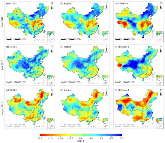
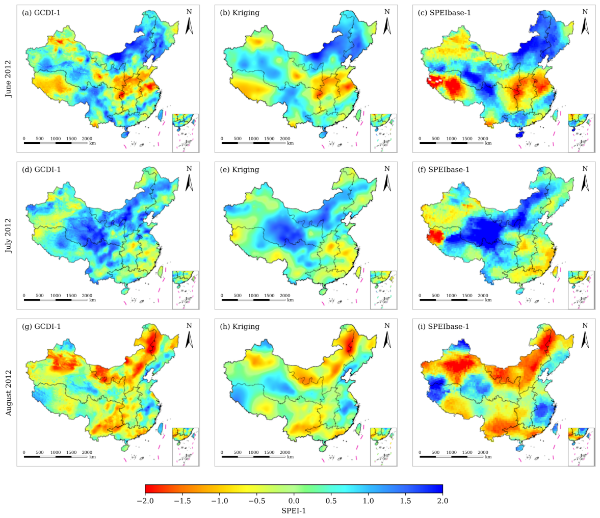
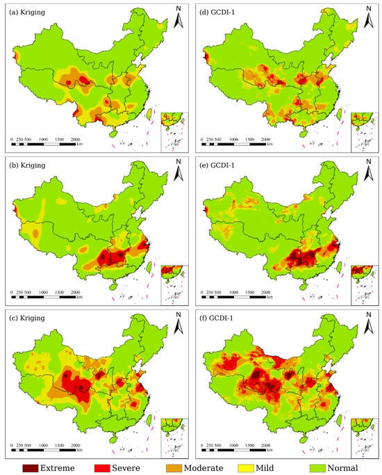
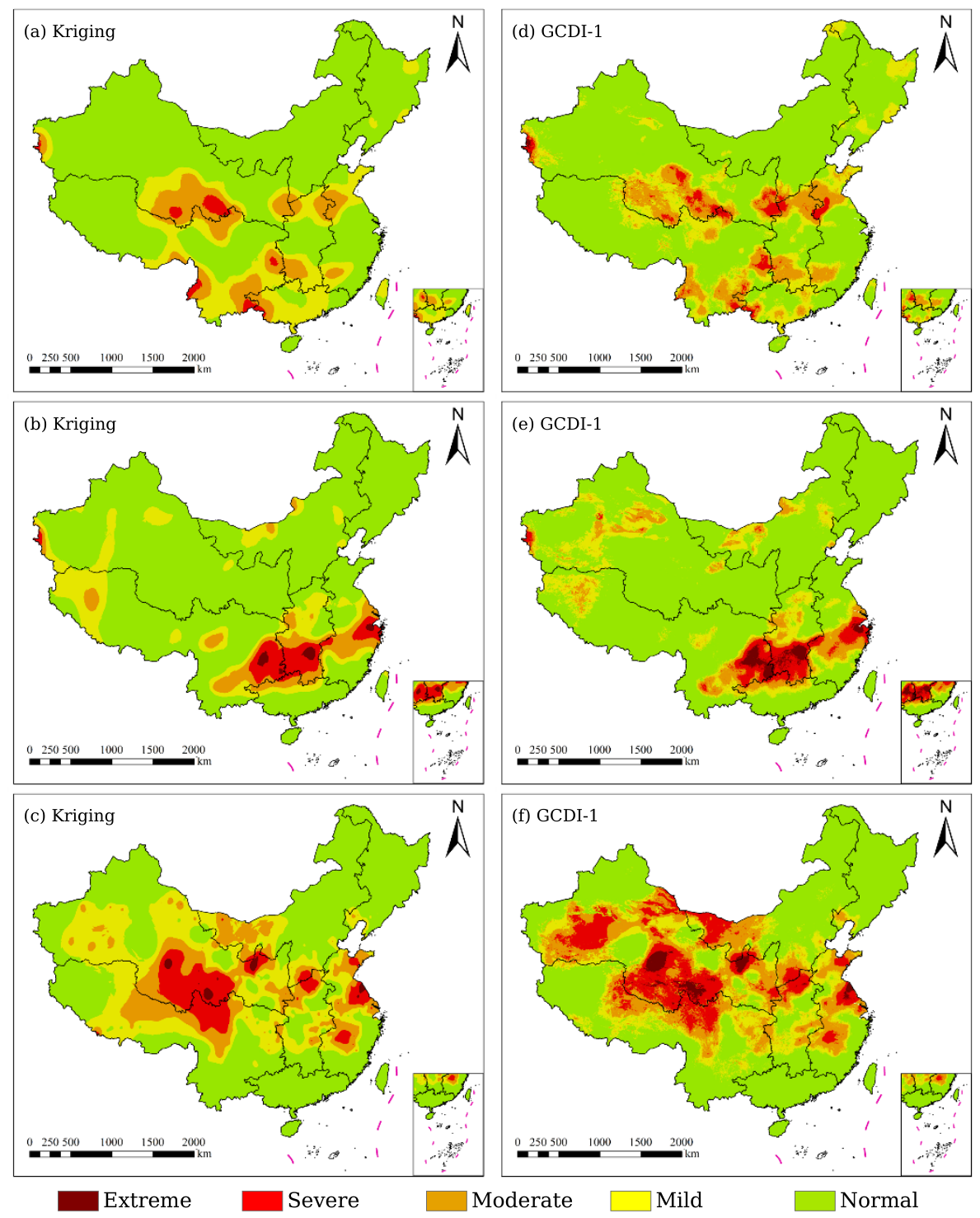
In terms of grid spacing, SPEIbase-1 is provided on a $0.5°$ grid, whereas GCDI-1 was generated on a 1-km output grid. Figure 11 compares the spatial distributions of GCDI-1, Kriging, and SPEIbase-1 in June, July, and August 2012. Overall, the three results exhibit broadly consistent regional drought patterns, but noticeable differences can be observed in their local spatial distributions. The Kriging results are relatively smooth because they are generated directly from station-based spatial interpolation, and some local variations and transition boundaries are consequently weakened. SPEIbase-1 also presents relatively coarse spatial patterns, which are consistent with its $0.5°$ grid spacing. In contrast, GCDI-1 shows richer local spatial variation and clearer spatial transitions between adjacent drought conditions on the 1-km output grid. The internal spatial heterogeneity of drought patterns is also more apparent in GCDI-1, particularly in areas where Kriging produces broad and smooth spatial distributions.

Figure 11. Spatial comparison of GCDI-1, Kriging, and SPEIbase-1 in June, July, and August 2012.

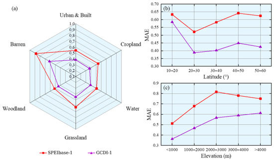
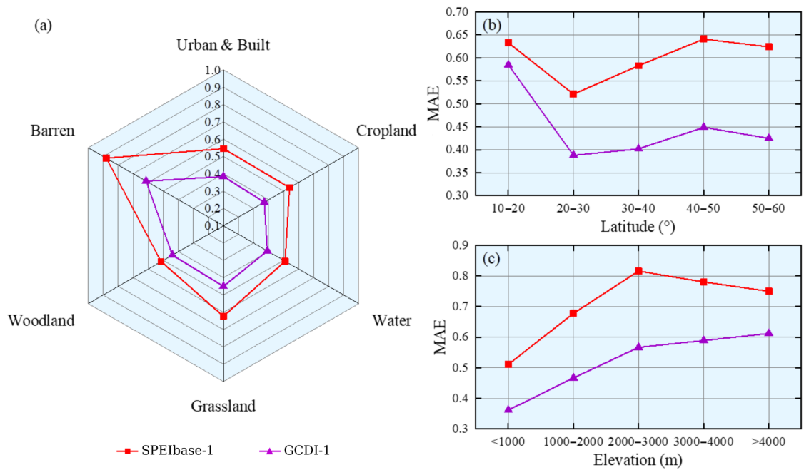
The station-referenced performance of GCDI-1 and SPEIbase-1 was further compared across different land cover types, latitude intervals, and elevation intervals, as shown in Figure 12. For land cover types (Figure 12a), barren land showed the highest $MAE$ for both products, with values of 0.607 for GCDI-1 and 0.894 for SPEIbase-1, whereas the lowest $MAE$ values were observed over cropland for GCDI-1 and water bodies for SPEIbase-1, with values of 0.372 and 0.510, respectively. The difference between the maximum and minimum $MAE$ was approximately 0.24 for GCDI-1 and 0.38 for SPEIbase-1, and GCDI-1 maintained lower $MAE$ values across all evaluated land cover classes. Across the evaluated latitude intervals (Figure 12b), the $MAE$ values of GCDI-1 ranged from 0.388 to 0.585, whereas those of SPEIbase-1 ranged from 0.521 to 0.633. GCDI-1 maintained lower $MAE$ values across all latitude intervals, while $MAE$ generally increased with increasing latitude within the 20–$50°$N range and showed relatively small variations within the 20–$40°$N range. As shown in Figure 12c, the station-referenced errors of both products also varied across elevation intervals. GCDI-1 maintained lower $MAE$ values than SPEIbase-1 across all evaluated elevation intervals, with a particularly large difference between the two products in the 2000–3000 m range. Overall, GCDI-1 showed lower station-referenced errors than SPEIbase-1 across the evaluated land cover, latitude, and elevation groups.

Figure 12. Comparison of station-level $MAE$ for GCDI-1 and SPEIbase-1 across (a) land cover types, (b) latitude intervals, and (c) elevation intervals during the temporally held-out 2011–2012 evaluation period.

5. Discussion

The experimental results indicate that GeoSPEI-1 provides the primary source of information for GCDI-1 estimation. In the input-combination experiments, GeoCSL using only the environmental variable groups (M + S + T) obtained an $RMSE$ of 0.735, whereas using GeoSPEI-1 alone reduced the $RMSE$ to 0.578. Incorporating the environmental variables together with GeoSPEI-1 further reduced the $RMSE$ to 0.546. Similar improvements were observed when GeoSPEI-1 was introduced into RF and DFNN. These results indicate that the geographically weighted neighboring-station information accounts for the major improvement in estimation performance, while the multi-source environmental variables provide additional complementary information rather than serving as the primary source of predictive information.

The spatial and temporal analyses further show that the performance improvement is not limited to the overall evaluation metrics. GeoCSL produced lower station-level errors at most evaluated locations and showed residual distributions that were generally closer to zero than those of the comparison models. The relationship between station density and station-level error nevertheless indicates that the spatial distribution of meteorological stations remains relevant to model performance. In the generated maps, GCDI-1 also exhibited greater local spatial variation than the Kriging interpolation and SPEIbase-1. This visual difference reflects the spatial representation produced by the integrated gridded inputs and GeoSPEI-1; however, it should not be interpreted as evidence that GCDI-1 has an effective spatial resolution of 1 km, because several input datasets have substantially coarser native grid spacing.

The GCDI-1 maps for 2013 were additionally compared with Kriging-interpolated SPEI-1 (Figure 13) and the drought conditions reported in the China Drought and Water Hazard Bulletin of 2013. The regional drought evolution represented by GCDI-1 from June to August was broadly consistent with the reported drought development in Southwest China and the middle and lower reaches of the Yangtze River. This comparison provides qualitative event-based support for the regional drought patterns represented by GCDI-1, but it is not treated as an independent quantitative validation of drought impacts.

Figure 13. Spatial comparison of Kriging-interpolated SPEI-1 and GCDI-1 from June to August 2013.

Several limitations should therefore be considered. First, GeoSPEI-1 is constructed from neighboring station-based SPEI-1 values, and the same overall station network is represented in the training and temporally held-out evaluation periods. Although the target station is excluded when constructing GeoSPEI-1 for station-based samples, the current 2011–2012 and 2013–2017 evaluations primarily assess temporal generalization at existing station locations rather than spatial transferability to previously unseen stations or regions. Second, the 1-km grid represents the output grid spacing of GCDI-1 rather than an effective spatial resolution of 1 km. Third, the present study does not quantitatively validate GCDI-1 against independent drought-related observations such as soil moisture observations, crop yield losses, or reported drought-affected areas. Future work will therefore focus on spatially independent evaluation and additional external drought-related observations.

6. Conclusions

This study developed a framework for GCDI generation by integrating multi-source RS data, meteorological station information, reanalysis variables, and the geographically weighted SPEI-related variable GeoSPEI-1 through the GeoCSL model. The framework was used to generate spatially continuous monthly GCDI-1 maps on a 1-km output grid over China. Ten-fold cross-validation using the 2001–2010 training samples yielded an $RMSE$ of 0.546, an $MAE$ of 0.407, and an R of 0.851 for GeoCSL. The input-combination experiments showed that GeoSPEI-1 was the primary contributor among the evaluated input variables, while the multi-source environmental variables provided additional complementary information. Comparisons across RF, DFNN, and CSL/GeoCSL further showed consistent performance improvements after GeoSPEI-1 was introduced, indicating that the contribution of GeoSPEI-1 was not limited to the GeoCSL architecture. Station-referenced evaluation using the temporally held-out 2011–2012 data showed that GCDI-1 achieved an $RMSE$ of 0.556 and an $MAE$ of 0.410 against station-based SPEI-1, compared with 0.562 and 0.421 for leave-one-station-out Kriging and 0.754 and 0.577 for SPEIbase-1, respectively. In addition, the station-referenced evaluation using 48,240 samples from 2013 to 2017 yielded an $RMSE$ of 0.593, an $MAE$ of 0.438, and an R of 0.840. These results support the use of geographically weighted neighboring-station information together with multi-source environmental variables for generating spatially continuous drought information over China.

Several limitations remain. Although GCDI-1 is generated on a 1-km output grid, several input datasets have substantially coarser native grid spacing, and the output grid should not be interpreted as an effective spatial resolution of 1 km. In addition, the current study has not quantitatively evaluated GCDI-1 against independent drought-related observations such as soil-moisture observations, crop yield losses, or reported drought-affected areas. Future work will therefore focus on additional independent drought-related observations and multi-timescale drought-index generation to further assess and extend the applicability of GCDI-1.

References

- Mishra, A.K.; Singh, V.P. A review of drought concepts. J. Hydrol. 2010, 391, 202–216. [Google Scholar] [CrossRef] [Scilit]
- Zhang, Q.; Shi, R.; Xu, C.Y.; Sun, P.; Yu, H.; Zhao, J. Multisource data-based integrated drought monitoring index: Model development and application. J. Hydrol. 2022, 615, 128644. [Google Scholar] [CrossRef] [Scilit]
- Chang, S.; Isaev, E.; Chen, H.; Wu, B.; Yan, N.; Ma, Z.; Meng, J. Exploring the Linkages Between Different Types of Drought and Their Impacts on Crop Production in Kyrgyzstan. IEEE J. Sel. Top. Appl. Earth Obs. Remote Sens. 2024, 17, 4566–4580. [Google Scholar] [CrossRef] [Scilit]
- Hazaymeh, K.; Hassan, Q.K. Remote sensing of agricultural drought monitoring: A state of art review. AIMS Environ. Sci. 2016, 3, 604–630. [Google Scholar] [CrossRef] [Scilit]
- Zhang, Z.; Xu, W.; Shi, Z.; Qin, Q. Establishment of a Comprehensive Drought Monitoring Index Based on Multisource Remote Sensing Data and Agricultural Drought Monitoring. IEEE J. Sel. Top. Appl. Earth Obs. Remote Sens. 2021, 14, 2113–2126. [Google Scholar] [CrossRef] [Scilit]
- Balti, H.; Ben Abbes, A.; Mellouli, N.; Farah, I.R.; Sang, Y.; Lamolle, M. A review of drought monitoring with big data: Issues, methods, challenges and research directions. Ecol. Inform. 2020, 60, 101136. [Google Scholar] [CrossRef] [Scilit]
- Azam, M.; Hunjra, A.I.; Bouri, E.; Tan, Y.; Al-Faryan, M.A.S. Impact of institutional quality on sustainable development: Evidence from developing countries. J. Environ. Manag. 2021, 298, 113465. [Google Scholar] [CrossRef] [Scilit] [PubMed]
- Ferrentino, E.; Polcari, M.; Silverii, F.; Bignami, C.; Nunziata, F.; Stramondo, S.; Migliaccio, M. On the joint use of SAR and meteo-climatological information to monitor the Po River under nominal and drought conditions. Int. J. Appl. Earth Obs. Geoinf. 2024, 133, 104095. [Google Scholar] [CrossRef] [Scilit]
- Tanriverdi, I.; Batmaz, İ. AI-driven US drought prediction using machine learning and deep learning. Clim. Dyn. 2025, 63, 249. [Google Scholar] [CrossRef] [Scilit]
- Zargar, A.; Sadiq, R.; Naser, B.; Khan, F.I. A review of drought indices. Environ. Rev. 2011, 19, 333–349. [Google Scholar] [CrossRef] [Scilit]
- Hao, Z.; AghaKouchak, A. Multivariate Standardized Drought Index: A parametric multi-index model. Adv. Water Resour. 2013, 57, 12–18. [Google Scholar] [CrossRef] [Scilit]
- Hao, Z.; Singh, V.P. Drought characterization from a multivariate perspective: A review. J. Hydrol. 2015, 527, 668–678. [Google Scholar] [CrossRef] [Scilit]
- Palmer, W.C. Meteorological Drought; US Department of Commerce, Weather Bureau: Washington, DC, USA, 1965; Volume 30.
- McKee, T.B.; Doesken, N.J.; Kleist, J. The relationship of drought frequency and duration to time scales. Am. Meteorol. Soc. 1993, 17, 179–183. [Google Scholar]
- Vicente Serrano, S.M.; Beguera, S.; Lpez-Moreno, J.I. Comment on “Characteristics and trends in various forms of the Palmer Drought Severity Index (PDSI) during 1900–2008” by Aiguo Dai. J. Geophys. Res. 2011, 116, D19112. [Google Scholar] [CrossRef] [Scilit]
- McKee, T.B.; Doesken, N.J.; Kleist, J. Drought monitoring with multiple time scales. Environ. Sci. 1995. [Google Scholar]
- Hayes, M.J.; Svoboda, M.D.; Wiihite, D.A.; Vanyarkho, O.V. Monitoring the 1996 drought using the standardized precipitation index. Bull. Am. Meteorol. Soc. 1999, 80, 429–438. [Google Scholar] [CrossRef] [Scilit]
- Vicente-Serrano, S.M.; Beguera, S.; Lpez-Moreno, J.I. A multiscalar drought index sensitive to global warming: The standardized precipitation evapotranspiration index. J. Clim. 2010, 23, 1696–1718. [Google Scholar] [CrossRef] [Scilit]
- Wen, J.; Zhang, X.; Wang, Y.; Wang, W. Effects of Drought in Multi-Time Scale on Wheat Crop in Eastern Agricultural Region of Qinghai Province. J. Irrig. Drain. 2016, 35, 92–97. [Google Scholar]
- Baez-Villanueva, O.M.; Zambrano-Bigiarini, M.; Miralles, D.G.; Beck, H.E.; Siegmund, J.F.; Alvarez-Garreton, C.; Verbist, K.; Garreaud, R.; Boisier, J.P.; Galleguillos, M. On the timescale of drought indices for monitoring streamflow drought considering catchment hydrological regimes. Hydrol. Earth Syst. Sci. 2024, 28, 1415–1439. [Google Scholar] [CrossRef] [Scilit]
- Zhang, Q.; Miao, C.; Su, J.; Gou, J.; Hu, J.; Zhao, X.; Xu, Y. A new high-resolution multi-drought-index dataset for mainland China. Earth Syst. Sci. Data 2025, 17, 837–853. [Google Scholar] [CrossRef] [Scilit]
- Zhao, Q.; Ma, Y.; Li, Z.; Yao, Y. Retrieval of a High-Precision Drought Monitoring Index by Using GNSS-Derived ZTD and Temperature. IEEE J. Sel. Top. Appl. Earth Obs. Remote Sens. 2021, 14, 8730–8743. [Google Scholar] [CrossRef] [Scilit]
- Liu, W.; Kogan, F. Monitoring regional drought using the vegetation condition index. Int. J. Remote Sens. 1996, 17, 2761–2782. [Google Scholar] [CrossRef] [Scilit]
- Jiao, W.; Tian, C.; Chang, Q.; Novick, K.A.; Wang, L. A new multi-sensor integrated index for drought monitoring. Agric. For. Meteorol. 2019, 268, 74–85. [Google Scholar] [CrossRef] [Scilit]
- Kogan, F.N. Global Drought Watch from Space. Bull. Am. Meteorol. Soc. 1997, 78, 621–636. [Google Scholar] [CrossRef] [Scilit]
- Kogan, F. Application of vegetation index and brightness temperature for drought detection. Adv. Space Res. 1995, 15, 91–100. [Google Scholar] [CrossRef] [Scilit]
- Zhou, X.; Wang, P.; Tansey, K.; Ghent, D.; Zhang, S.; Li, H.; Wang, L. Drought Monitoring Using the Sentinel-3-Based Multiyear Vegetation Temperature Condition Index in the Guanzhong Plain, China. IEEE J. Sel. Top. Appl. Earth Obs. Remote Sens. 2020, 13, 129–142. [Google Scholar] [CrossRef]
- Zhou, L.; Wu, J.; Zhang, J.; Leng, S.; Liu, M.; Zhang, J.; Zhao, L.; Zhang, F.; Shi, Y. The Integrated Surface Drought Index (ISDI) as an Indicator for Agricultural Drought Monitoring: Theory, Validation, and Application in Mid-Eastern China. IEEE J. Sel. Top. Appl. Earth Obs. Remote Sens. 2013, 6, 1254–1262. [Google Scholar] [CrossRef] [Scilit]
- Kogan, F.N. Operational Space Technology for Global Vegetation Assessment. Bull. Am. Meteorol. Soc. 2001, 82, 1949–1964. [Google Scholar] [CrossRef] [Scilit]
- Guo, H.; Bao, A.; Liu, T.; Ndayisaba, F.; Jiang, L.; Zheng, G.; Chen, T.; De Maeyer, P. Determining variable weights for an Optimal Scaled Drought Condition Index (OSDCI): Evaluation in Central Asia. Remote Sens. Environ. 2019, 231, 111220. [Google Scholar] [CrossRef] [Scilit]
- Brown, J.F.; Wardlow, B.D.; Tadesse, T.; Hayes, M.J.; Reed, B.C. The Vegetation Drought Response Index (VegDRI): A New Integrated Approach for Monitoring Drought Stress in Vegetation. GIScience Remote Sens. 2008, 45, 16–46. [Google Scholar] [CrossRef] [Scilit]
- Rhee, J.; Im, J.; Carbone, G.J. Monitoring agricultural drought for arid and humid regions using multi-sensor remote sensing data. Remote Sens. Environ. 2010, 114, 2875–2887. [Google Scholar] [CrossRef] [Scilit]
- Khosravi, Y.; Homayouni, S.; St-Hilaire, A. An integrated dryness index based on geographically weighted regression and satellite earth observations. Sci. Total Environ. 2024, 911, 168807. [Google Scholar] [CrossRef] [Scilit] [PubMed]
- Bayissa, Y.A.; Tadesse, T.; Svoboda, M.; Wardlow, B.; Poulsen, C.; Swigart, J.; Andel, S.J.V. Developing a satellite-based combined drought indicator to monitor agricultural drought: A case study for Ethiopia. GIScience Remote Sens. 2019, 56, 718–748. [Google Scholar] [CrossRef] [Scilit]
- Wei, W.; Zhang, J.; Zhou, J.; Zhou, L.; Xie, B.; Li, C. Monitoring drought dynamics in China using Optimized Meteorological Drought Index (OMDI) based on remote sensing data sets. J. Environ. Manag. 2021, 292, 112733. [Google Scholar] [CrossRef] [Scilit] [PubMed]
- Belayneh, A.; Adamowski, J. Drought forecasting using new machine learning methods. J. Water Land Dev. 2013, 18, 3–12. [Google Scholar] [CrossRef] [Scilit]
- Liu, R.; Yin, J.; Slater, L.; Kang, S.; Yang, Y.; Liu, P.; Guo, J.; Gu, X.; Zhang, X.; Volchak, A. Machine-learning-constrained projection of bivariate hydrological drought magnitudes and socioeconomic risks over China. Hydrol. Earth Syst. Sci. 2024, 28, 3305–3326. [Google Scholar] [CrossRef] [Scilit]
- Shen, R.; Huang, A.; Li, B.; Guo, J. Construction of a drought monitoring model using deep learning based on multi-source remote sensing data. Int. J. Appl. Earth Obs. Geoinf. 2019, 79, 48–57. [Google Scholar] [CrossRef] [Scilit]
- Raza, M.O.; Mahoto, N.A.; Al Reshan, M.S.; Alqazzaz, A.; Rajab, A.; Shaikh, A. Drought detection in satellite imagery: A layered ensemble machine learning approach. Int. J. Comput. Intell. Syst. 2025, 18, 161. [Google Scholar] [CrossRef] [Scilit]
- Houmma, I.H.; Gadal, S.; Mansouri, L.E.; Garba, M.; Gbetkom, P.G.; Barkawi, M.B.M.; Hadria, R. A new multivariate agricultural drought composite index based on random forest algorithm and remote sensing data developed for Sahelian agrosystems. Geomat. Nat. Hazards Risk 2023, 14, 2223384. [Google Scholar] [CrossRef] [Scilit]
- Başakın, E.E.; Stoy, P.C.; Demirel, M.C.; Ozdogan, M.; Otkin, J.A. Combined Drought Index Using High-Resolution Hydrological Models and Explainable Artificial Intelligence Techniques in Türkiye. Remote Sens. 2024, 16, 3799. [Google Scholar] [CrossRef] [Scilit]
- Xu, Z.; Sun, H.; Zhang, T.; Xu, H.; Wu, D.; Gao, J. The high spatial resolution Drought Response Index (HiDRI): An integrated framework for monitoring vegetation drought with remote sensing, deep learning, and spatiotemporal fusion. Remote Sens. Environ. 2024, 312, 114324. [Google Scholar] [CrossRef] [Scilit]
- Belayneh, A.; Adamowski, J.; Khalil, B.; Ozga-Zielinski, B. Long-term SPI drought forecasting in the Awash River Basin in Ethiopia using wavelet neural network and wavelet support vector regression models. J. Hydrol. 2014, 508, 418–429. [Google Scholar] [CrossRef] [Scilit]
- Guzmán, S.M.; Paz, J.O.; Tagert, M.L.M.; Mercer, A.E.; Pote, J.W. An integrated SVR and crop model to estimate the impacts of irrigation on daily groundwater levels. Agric. Syst. 2018, 159, 248–259. [Google Scholar] [CrossRef] [Scilit]
- Di Persio, L.; Fraccarolo, N. Energy Consumption Forecasts by Gradient Boosting Regression Trees. Mathematics 2023, 11, 1068. [Google Scholar] [CrossRef] [Scilit]
- Di Persio, L.; Fraccarolo, N.; Veronese, A. Wind Energy Production in Italy: A Forecasting Approach Based on Fractional Brownian Motion and Generative Adversarial Networks. Mathematics 2024, 12, 2105. [Google Scholar] [CrossRef] [Scilit]
- Li, X.; Jia, H.; Wang, L. Remote Sensing Monitoring of Drought in Southwest China Using Random Forest and eXtreme Gradient Boosting Methods. Remote Sens. 2023, 15, 4840. [Google Scholar] [CrossRef] [Scilit]
- Beguería, S.; Vicente-Serrano, S.M.; Angulo-Martínez, M. A Multiscalar Global Drought Dataset: The Speibase: A New Gridded Product for the Analysis of Drought Variability and Impacts. Bull. Am. Meteorol. Soc. 2010, 91, 1351–1354. [Google Scholar] [CrossRef] [Scilit]
- DeGaetano, A.T.; Belcher, B.N.; Noon, W. Temporal and Spatial Interpolation of the Standardized Precipitation Index for Computational Efficiency in the Dynamic Drought Index Tool. J. Appl. Meteorol. Climatol. 2015, 54, 795–810. [Google Scholar] [CrossRef] [Scilit]
- Hirwa, H. Review and synthesis: Dynamism of classical and holistic drought indices and indicators. Front. Water 2025, 7, 1672070. [Google Scholar] [CrossRef] [Scilit]
- Allen, R.G.; Pereira, L.S.; Raes, D.; Smith, M. Crop Evapotranspiration-Guidelines for Computing Crop Water Requirements-FAO Irrigation and Drainage Paper 56; Fao: Rome, Italy, 1998; Volume 300, p. D05109. [Google Scholar]
- Roberts, D.R.; Bahn, V.; Ciuti, S.; Boyce, M.S.; Elith, J.; Guillera-Arroita, G.; Hauenstein, S.; Lahoz-Monfort, J.J.; Schröder, B.; Thuiller, W.; et al. Cross-validation strategies for data with temporal, spatial, hierarchical, or phylogenetic structure. Ecography 2017, 40, 913–929. [Google Scholar] [CrossRef] [Scilit]
- Valavi, R.; Elith, J.; Lahoz-Monfort, J.J.; Guillera-Arroita, G. blockCV: An R package for generating spatially or environmentally separated folds for k-fold cross-validation of species distribution models. bioRxiv 2018. [Google Scholar] [CrossRef] [Scilit]
- Glorot, X.; Bengio, Y. Understanding the Difficulty of Training Deep Feedforward Neural Networks. In Proceedings of the Thirteenth International Conference on Artificial Intelligence and Statistics, Sardinia, Italy, 13–15 May 2010; Volume 9, pp. 249–256. [Google Scholar]
Disclaimer/Publisher’s Note: The statements, opinions and data contained in all publications are solely those of the individual author(s) and contributor(s) and not of MDPI and/or the editor(s). MDPI and/or the editor(s) disclaim responsibility for any injury to people or property resulting from any ideas, methods, instructions or products referred to in the content. |
© 2026 by the authors. Licensee MDPI, Basel, Switzerland. This article is an open access article distributed under the terms and conditions of the Creative Commons Attribution (CC BY) license.