


Highlights
What are the main findings?
- The proposed ABS-Net adaptive band selection network effectively eliminates redundant spectral bands and retains critical diagnostic features; high-contribution bands are concentrated in 380–560 nm visible and 700–1000 nm near-infrared regions for archaeological stratigraphic discrimination.
- Global PCA dimensionality reduction discards subtle inter-stratum spectral gradients, resulting in degraded classification performance for spectrally similar archaeological cultural layers.
What are the implications of the main findings?
- Hyperspectral deep learning mitigates subjective bias of manual stratigraphic interpretation and delivers an objective technical reference for the intelligent delineation of archaeological profiles, though multi-site datasets are required to validate model generalisation.
- The adaptive band selection paradigm offers transferable inspiration for other hyperspectral classification tasks facing severe band redundancy and weak inter-class spectral differences.
Abstract
Archaeological stratigraphy serves as the core foundation for establishing archaeological chronological sequences, clarifying ancient human activity patterns, and revealing the evolution of human–land relationships. Current field stratigraphic delineation mainly relies on manual visual observation and empirical judgement, which suffers from strong subjectivity and poor repeatability. It is difficult to accurately identify quasi-homogeneous archaeological strata with similar paedogenic backgrounds and soil characteristics, easily resulting in stratigraphic misclassification and boundary misjudgement. Hyperspectral imaging technology can effectively capture subtle spectral differences in soil physicochemical components and support the refined identification of homogeneous strata, whereas its practical application is restricted by high data dimensionality, severe band redundancy, and insufficient targeted extractions of effective features. Taking five typical archaeological deposits, including Warring States–Han, Song–Yuan, and Ming–Qing cultural layers, ash pits, and undisturbed subsoil, this study constructs a spectral–spatial collaborative deep learning model (ABS-Net) with an adaptive band selection module based on field-measured hyperspectral data of archaeological profiles. The proposed model realises the automatic mining of subtle spectral features and intelligent stratigraphic classification. Comparative experiments with multiple state-of-the-art hyperspectral classification models demonstrate that ABS-Net achieves competitive and stable classification accuracy. This study verifies the feasibility and application potential of combining hyperspectral remote sensing with deep learning for intelligent stratigraphic classification, providing a novel technical reference for intelligent stratigraphic interpretation in field archaeology.
1. Introduction
As the fundamental core of archaeology, archaeological stratigraphy provides an essential theoretical and methodological basis for constructing the chronological and spatial framework of archaeological research, as well as for interpreting paleohuman activities and environmental evolution [1]. Through systematic analysis of the stacking order and spatial juxtaposition of cultural layers at archaeological sites, the dynamic interactions between anthropogenic activities and natural environmental changes can be quantitatively and qualitatively revealed [2,3].
In conventional sedimentary environments, site deposits generally follow the superposition law, i.e., older strata underlie younger ones. Nevertheless, long-term anthropogenic disturbance and natural exogenous modification frequently alter original stratigraphic structures, resulting in blurred stratigraphic boundaries, mixed deposits, and disordered layer sequences, which substantially increases the difficulty of stratigraphic identification and interpretation [4,5]. Current field stratigraphic division predominantly relies on conventional artificial discrimination [6]. Archaeologists delineate vertical stratigraphic sequences according to macroscopic differences in soil texture, colour, structure, and sedimentary inclusions (e.g., pottery shards, stone artefacts, animal bones, and charcoal fragments) [7]. However, this approach is highly dependent on field experience and prior knowledge, leading to substantial subjectivity and empirical uncertainty. In particular, adjacent strata with similar paedogenic backgrounds and subtle physicochemical differences exhibit high interlayer similarity and intralayer variability in soil composition and macroscopic characteristics [8,9]. Such inherent similarities hinder the precise differentiation of subtle stratigraphic variations via artificial identification, thereby inevitably causing stratigraphic misclassification and boundary misjudgement.
With the rapid development of digital and technological archaeology, digital techniques, including three-dimensional scanning, GIS modelling and remote sensing detection, have been progressively applied to field archaeological practice, promoting the transformation of archaeological stratigraphic research from traditional experience-driven qualitative discrimination to data-oriented quantitative analysis [10]. Among these techniques, hyperspectral imaging has emerged as a cutting-edge method for refined stratigraphic identification due to its unique advantages of integrated spectral–spatial mapping, non-destructive detection, and high spectral and spatial resolution [8,9]. Different from conventional RGB and multispectral remote sensing that only acquire discrete band surface information, hyperspectral technology can collect hundreds of continuous narrow-band spectral data in the visible-to-short-wave infrared range [11,12]. It is capable of capturing subtle spectral response differences in soil physicochemical components, including soil organic matter, free iron oxide, clay minerals, carbonates, salts and humus, thereby effectively distinguishing quasi-homogeneous archaeological strata that are indistinguishable to the naked eye and conventional imaging methods [13,14,15]. This provides reliable data support for the quantitative identification of stratigraphic subtle differences [9,16]. Currently, hyperspectral technology has been widely adopted in various archaeological scenarios, such as mural pigment identification [17,18,19], stone relic weathering monitoring [20,21], bronze corrosion analysis [22], ancient site detection [23,24] and paleoenvironmental reconstruction [25,26]. Nevertheless, these conventional applications still suffer from inherent technical limitations, including severe data redundancy and insufficient targeted feature extraction.
Hyperspectral data contain hundreds of adjacent bands with strong linear correlation [27]. This high band redundancy not only increases data storage and computational costs and reduces model training efficiency, but also accumulates noise interference and weakens the saliency of effective spectral features, ultimately limiting the classification accuracy of archaeological scenarios [28]. Principal component analysis (PCA) is one of the most widely used dimensionality reduction and de-redundancy methods for hyperspectral data processing [29,30,31]. It compresses spectral dimensions through global linear transformation and is well suited for conventional remote sensing land-cover classification tasks [32]. Moreover, random noise caused by measurement errors and outliers contained in the dataset will severely interfere with the solution process, resulting in biased or even misleading principal components [33,34]. In addition, the number of retained principal components is generally determined by empirical rules, which tends to lose the subtle and fine spectral features required to distinguish quasi-homogeneous strata. In addition, the transformed principal components lose the physical semantics of original spectral bands with low interpretability, making it impossible to identify dominant bands for stratigraphic discrimination [11,35,36]. Compared with PCA-based linear transformation methods, band selection (BS) techniques directly screen optimal band subsets with explicit physical significance from the original hyperspectral data, effectively avoiding the lack of physical interpretability inherent in principal component transformation [37,38]. Existing BS methods can be divided into unsupervised and supervised categories [28]. Unsupervised methods require no labelled samples and select bands based on spectral statistical characteristics [38]. However, they only evaluate individual band information and ignore the synergistic effects of band combinations, tending to retain highly correlated and redundant adjacent bands [39]. In contrast, supervised BS methods iterate and optimise by relying on prior sample category information to maximise spectral separability among land-cover types and improve classification performance, thus exhibiting better targeting and practicality [37]. Such methods are plagued by limited architectural compatibility, heavy reliance on manual annotations, and high susceptibility to labelling noise [40].
Deep learning techniques, which eliminate the reliance on manual prior knowledge and enable autonomous mining of implicit complex features, are capable of fully extracting joint spectral–spatial characteristics from hyperspectral data [41,42], providing a novel technical solution for the refined classification of archaeological strata. Currently, convolutional neural networks (CNN) and Transformer architectures dominate the intelligent classification of hyperspectral images. CNNs extract local spatial texture and spectral features via convolutional operators [29,43] and integrate residual structures to alleviate gradient vanishing caused by increased network depth, realising the fusion and extraction of multi-scale features [11,35]. However, restricted by the local receptive field mechanism, CNNs fail to model sequential spectral information and capture long-range spectral dependencies and subtle spectral variations. They also struggle to establish global spatial dependencies, easily leading to the loss of contextual information and feature redundancy [12,31]. Although recurrent neural networks (RNNs) can extract features according to spectral sequences, they suffer from severe gradient vanishing issues and cannot effectively capture long-range spectral dependencies and subtle feature differences [44,45]. By contrast, Transformer models break the local receptive field limitation of CNNs through a multi-head self-attention mechanism, which efficiently models long-range spectral sequence correlations and global spatial dependencies, and has been widely applied in hyperspectral classification tasks [12]. Benefiting from this advantage, Transformer models outperform traditional machine learning and CNN-based methods. Furthermore, recent advanced hyperspectral networks including Representative Spectral Correlation Network [46], Semantic-Guided Fusion Network [47] and MSFMamba [48] achieve promising performance by exploring effective spectral feature mining. Nevertheless, these architectures are primarily optimised for conventional land-cover scenarios with significant spectral differences, such as vegetation, water bodies, and construction lands. These models are poorly adapted to the unique characteristics of archaeological strata, including similar paedogenic backgrounds, subtle spectral discrepancies, and ambiguous interlayer boundaries. Targeted research focusing on refined archaeological stratigraphic classification remains insufficient.
To address the current challenges in archaeological stratigraphic classification, including strong subjectivity of manual discrimination, low accuracy in distinguishing quasi-homogeneous strata, and the loss of subtle spectral features caused by conventional dimensionality reduction and band selection methods with poor compatibility with deep learning frameworks, this study proposes a novel spectral–spatial collaborative classification model (ABS-Net) for refined stratigraphic identification. Based on hyperspectral data collected from field archaeological profiles, the proposed model integrates an adaptive band selection module and a spatial attention mechanism to optimise feature extraction for subtle stratigraphic differences. Furthermore, this study systematically compares the performance and stratigraphic adaptability of two mainstream deep learning frameworks, CNN and Transformer, in archaeological stratigraphic classification. This work aims to break the empirical limitations of traditional manual stratification, realise the intelligent classification of archaeological strata, and provide an effective technical reference for refined stratigraphic division in field archaeology.
2. Materials and Methods
2.1. Materials
Hyperspectral data of archaeological strata were acquired using a Headwall hyperspectral imaging camera (Headwall Photonics Inc., Bolton, MA, USA) (Figure 1a). The data acquisition system consisted of a hyperspectral camera, a motorised rotating pan–tilt head, and a triangular support tripod. Field measurements were conducted on the west-wall profile of an archaeological test pit at 13:30 on 1 April 2025. The profile preserves continuous sedimentary sequences ranging from the Warring States–Han period to modern soil accumulation (Table 1), and all stratigraphic units were systematically divided by professional archaeologists according to sedimentary characteristics (Figure 1d). Before formal data acquisition, the tilt angle, initial angle and scanning range of the pan–tilt platform were configured according to device parameters. Dark current correction and whiteboard reference correction were sequentially implemented for spectral calibration. Equipped with a motorised pan–tilt unit, the system adopts a push-broom linear scanning mode for data collection. The hyperspectral sensor provides an original spectral sampling interval of 0.8 nm, covering 775 spectral channels within the visible and near-infrared range of 380–1000 nm. The established dataset contains 939 spatial pixels and 775 spectral bands. The acquired hyperspectral data were stored as three-dimensional data cubes with dimensions of height, width, and channel, representing spatial vertical extent, spatial horizontal extent, and spectral band number, respectively.
Figure 1.
Hyperspectral images and archaeological strata. (a) Hyperspectral data acquisition device; (b) field photograph of the stratigraphic profile; (c) 3D cube of hyperspectral image (R: 438 nm, G: 546 nm, B: 700 nm); (d) stratigraphic labelling result.
Table 1.
Abbreviations and chronological information of different archaeological strata.
In this study, the modern cultivated topsoil (Layer L1) was artificially removed prior to data collection, and the remaining L2, L3, and L4 layers were retained as anthropogenic cultural deposits (Table 1). Cultural layers represent horizontal sedimentary accumulations formed by long-term human activities, containing evenly distributed archaeological remains such as pottery shards, stone artefacts, charcoal fragments, and animal bones. Their superposition relationships establish the chronological sequence of the archaeological site and serve as the fundamental basis for determining site age and cultural characteristics. These cultural deposits are commonly truncated by later archaeological features including pits, house foundations, and tombs. In addition, pit features (H) are artificially excavated depressions originally constructed for waste disposal, storage, soil extraction, or ritual activities, which were subsequently backfilled naturally or artificially. Characterised by clear boundaries and dense relic assemblages, pits typically cut through earlier cultural layers and undisturbed subsoil, providing critical evidence for reconstructing ancient human behaviours and livelihood patterns. Undisturbed subsoil (S) refers to pristine natural sediment formed prior to human occupation without any anthropogenic remains, which marks the basal boundary of archaeological excavation and the bottom of the cultural stratigraphic sequence. Cultural layers, pit deposits, and subsoil exhibit significant differences in soil texture, morphological characteristics, inclusions, and stratigraphic relationships, forming the primary foundation for field stratigraphic identification and chronological interpretation.
2.2. Proposed Method
2.2.1. Hyperspectral Image Preprocessing
- Savitzky–Golay Filtering
Hyperspectral data of archaeological strata contain both stratigraphic texture information in the spatial dimension and sediment physicochemical signatures in the spectral dimension, showing strong coupled spectral–spatial characteristics. Affected by sensor system noise, environmental interference and subtle textural variations in strata, the original hyperspectral cubes suffer from uneven noise distribution across bands. Low signal-to-noise ratio bands are prone to spectral distortion and feature degradation, which seriously impairs the accurate identification of layers and homogeneous sedimentary strata.
Conventional standalone spatial filtering or spectral filtering methods have obvious drawbacks: spatial filtering tends to over-smooth faint stratigraphic boundaries, while band-wise spectral filtering fails to suppress random noise using spatial neighbourhood constraints. The Savitzky–Golay (SG) filter can effectively suppress noise interference while preserving the prominent morphological features of the original signal to the greatest extent [23,49]. Considering the unique spectral–spatial coupling characteristics of archaeological hyperspectral data, this study adopts the SG filter with second-order polynomial fitting. A 5 × 5 spatial window and a 20-band spectral window are configured to implement three-dimensional joint spectral–spatial filtering for preprocessing. The filtering procedure sequentially performs row-wise spatial smoothing, column-wise spatial smoothing, and spectral-axis smoothing. Specifically, spatial neighbourhood smoothing is applied to each single band to remove salt-and-pepper noise within homogeneous strata while precisely preserving stratigraphic boundary features. Pixel-wise fitting and optimisation are then conducted along the spectral dimension to effectively reduce random fluctuations and spectral curve distortion. This method achieves an optimal trade-off among noise suppression, stratigraphic edge preservation and fidelity of sediment spectral features.
- 2.
- Signal-to-Noise Ratio Estimation
Signal-to-noise ratio (SNR, unit: dB) serves as a reliable quantitative indicator for evaluating the quality of archaeological hyperspectral data and the effectiveness of preprocessing algorithms, which avoids the subjective uncertainty of qualitative visual judgement based on spectral curve smoothness. SNR quantifies the power ratio of valid target reflection signals to random noise introduced by sensors and environmental interference. A higher SNR indicates weaker noise interference on genuine spectral signals, and the observed band reflectance is closer to the real spectral response of stratigraphic sediments. In this study, a 5 × 5 sliding window consistent with the filtering spatial scale is adopted to achieve unbiased band-by-band SNR estimation, which can accurately separate valid stratigraphic spectral signals from sensor random noise. Specifically, for each spectral band λ, a local neighbourhood window Ω centred at pixel (x,y) is constructed, and the mean reflectance within the window is calculated to represent the stable local valid signal:
where Rλ denotes the reflectance value of pixel (i,j) in band λ; M is the total number of pixels inside the window, and M = 25 in this work.
An unbiased standard deviation with degrees of freedom M − 1 is further used to estimate the amplitude of random noise and reduce statistical bias induced by limited sample size:
Stratification textures and stratigraphic boundaries contain structural information that would interfere with pure noise statistics. Due to the inherent spatial heterogeneity and texture variations in soil, fully homogeneous spectral regions rarely exist in archaeological stratigraphic profiles. In this study, regions with relatively low local variance are selected to calculate the signal-to-noise ratio (SNR). The obtained SNR values are only used for the relative evaluation of dataset quality, rather than representing the absolute noise level of archaeological strata. Following the conventional decibel definition widely used in optical remote sensing, the band-wise SNR is formulated as:
where μ(λ) and σ(λ) refer to the mean signal value and noise standard deviation derived from the optimal homogeneous regions, respectively. Established on the spectral amplitude ratio, this formula can objectively quantify the data quality of each hyperspectral band and quantitatively evaluate the improvement brought by the filtering denoising preprocessing.
2.2.2. Adaptive Band Selection Net (ABS-Net)
The proposed ABS-Net architecture consists of three core components: an adaptive band selection module (ABS), a heterogeneous convolution and multi-head attention fusion module (HetConv-MHA), and an MLP classification head. The overall network framework is illustrated in Figure 2a. The input of the model is a hyperspectral data cube with the dimension of X ∈ ℝb×c×h×w. Firstly, the ABS module adaptively screens high-discriminative valid bands and eliminates redundant and noisy bands (Figure 2b). Secondly, point-wise convolution is adopted for dimensionality reduction, heterogeneous convolution is used to extract local spatial features, and grouped multi-head attention is integrated to capture long-range global spectral–spatial dependencies (Figure 2c). Finally, global average pooling is applied for feature aggregation, followed by a multi-layer perceptron to implement the final classification of archaeological strata (Figure 2d).
Figure 2.
Overall architecture of the proposed ABS-Net. (a) Adaptive Band Selection Module; (b) Heterogeneous Convolution and Multi-Head Attention Joint Module; (c) Classification Head. (d) Classification Head.
- 3.
- Adaptive Band Selection Module
Hyperspectral imagery consists of hundreds of highly redundant consecutive bands, and fixed rule-based band selection methods fail to adapt to hyperspectral datasets collected from different archaeological profiles with variable noise levels. Inspired by previous studies [17,18], this study designs an adaptive band screening module based on learnable codebook clustering (Figure 2b). Without manual prior rules for band selection, the module automatically learns to generate band importance weight masks according to the intrinsic spectral distribution of data, retains high-discriminative valid bands at a preset proportion, and eliminates highly redundant and noise-contaminated bands.
- (1)
- Spectral Feature Embedding
Grouped convolution (GWC) is first applied to perform spatial preprocessing on each band of the input hyperspectral cube X ∈ ℝb×c×h×w. Subsequently, 1 × 1 point-wise convolution (PWC) is used for spectral feature projection to obtain embedded features X∗ ∈ ℝb×c×h×w, formulated as:
where BN denotes batch normalisation and Relu is the nonlinear activation function.
Y = BN (Relu(GWC(X)))
X∗ = BN (Relu(PWC(Y)))
X∗ = BN (Relu(PWC(Y)))
- (2)
- Codebook Attention Generation
A set of learnable global spectral codebook centres C is introduced to capture global spectral statistical characteristics of the entire profile. The L2 distance between pixel-wise spectral vectors and codebook vectors is calculated to measure feature similarity: a smaller L2 distance indicates higher spectral similarity, while a larger distance implies greater spectral discrepancy. The embedded feature X∗ ∈ ℝb×D×h×w is reshaped into a 2D matrix Zreshape ∈ ℝbn×D, where b is the batch size, n = h × w represents the total number of pixels per batch, and the feature dimension D equals the original band number c. The learnable codebook centres are defined as C ∈ ℝK×D (K = number of codebooks), together with a scaling coefficient vector S ∈ ℝK. The final output distance matrix is Ddis ∈ ℝb×n×K. To avoid prohibitive computational cost caused by double nested loops, vectorized matrix operation is adopted to compute the raw Euclidean distance for spatially flattened features Zreshape ∈ ℝbn×D:
in which is the squared L2 norm of pixel features, and is the squared L2 norm of codebook features. This parallel computing strategy drastically reduces codebook matching overhead and accommodates high-resolution archaeological hyperspectral data. Direct adoption of raw L2 distance has two drawbacks: all codebook centres share an identical distance metric and cannot differentially characterise distributions of distinct spectral prototypes; In addition, large raw distance values easily lead to gradient saturation after Softmax activation, resulting in the low discrimination of attention weights. To address this issue, a learnable scaling vector S is introduced to adaptively weight and scale distance distributions across different codebook channels, enlarging the distance gap between valid and invalid bands and improving the discriminability of attention coefficients:
Ddis = S⊙Draw
The 2D distance matrix is restored to a 3D tensor Ddis ∈ ℝb×n×K, which is normalised by Softmax to yield the attention weight matrix A ∈ ℝb×n×K representing pixel-wise weights relative to global codebook prototypes:
A = Softmax(reshape(Ddis))
- (3)
- Global Spectral Feature Aggregation
Weighted summation is performed on residuals between pixel spectra and codebook centres guided by attention weights A ∈ ℝb×n×K. Discrete local pixel spectra are aggregated into globally unified spectral representations, producing codebook aggregated features E ∈ ℝb×K×D:
The aggregated features are sequentially processed by batch normalisation and Relu activation, followed by summation along the codebook dimension to derive the global spectral vector Esum ∈ ℝb×D. This global representation reflects the overall spectral statistics of the whole profile and serves as the basis for subsequent band importance evaluation:
Esum = Sum(Relu(BN(E))
- (4)
- Band Importance Scoring and Mask Generation
To study the influence of spectral resolution (band width) on stratigraphic classification performance, our experiments do not directly modify the spectral resolution of the raw data. Instead, band masks with widths of 2 nm, 4 nm, and 8 nm are constructed to simulate multi-resolution scenarios. We calculate band importance scores using a linear layer combined with the Sigmoid function and adopt a continuous soft mask to replace the conventional binary hard mask. With nearest-neighbour interpolation for mask construction and dimension alignment, element-wise operations between the mask and feature maps screen discriminative valid bands and suppress noisy bands, achieving adaptive selection of the optimal band subset.
Band importance scores are generated via a linear layer followed by the Sigmoid function:
where σ denotes the sigmoid function constraining scores within the range [0,1]; a higher score indicates richer discriminative spectral information for stratigraphic identification; Flinear is the fully connected layer adapted to the corresponding band width.
γ = σ(Flinear(Esum))
Given the predefined retention ratio p of valid bands, the total number of reserved bands is calculated via the ceiling function . The TopK algorithm sorts the band importance scores γ, extracts the indices idx of high-score bands, and retains the corresponding spectral channels via these indices to realise the adaptive selection of the optimal band subset.
where is the index matrix of screened dominant bands. Different from traditional binary hard masks with values 0 or 1, a continuous soft mask strategy is adopted herein: positions indexed by selected bands are assigned their original importance scores, while redundant unselected bands are set to zero. A 2D mask M2d is generated through the scatter operation:
Nearest-neighbour linear interpolation upsamples the low-dimensional mask back to the original spectral dimension and expands it into a 4D tensor M ∈ ℝb×c×1×1 for dimension consistency:
M = LinearInterpolate(M2d)
Element-wise multiplication is conducted between the preceding embedded feature Y and band mask M to weight-enhance high-value bands and suppress noisy redundant bands. The adaptive band selection is finally accomplished with the output screened feature:
- 4.
- Heterogeneous Convolution and Multi-Head Attention Joint Module
The input features are first fed into a lightweight heterogeneous convolution (HetConv) block, which integrates grouped spatial convolution and spectral convolution in a parallel manner, followed by batch normalisation (BN) and Relu activation. Afterwards, a joint spatial–spectral attention module is employed to model global spatial correlations within hyperspectral data (Figure 2c). All convolutional operations adopt grouped convolution design to reduce the number of parameters and floating-point operations. Meanwhile, learnable scaling coefficients are introduced to adaptively adjust the distribution of attention weights.
- (1)
- Heterogeneous Convolution Module
The original hyperspectral data contains up to 750 spectral bands, which suffers from severe band redundancy, strong channel coupling and sparse valid feature distribution. At the network input layer, a 1 × 1 point-wise convolution (PWC) is applied to perform channel dimensionality reduction on the high-dimensional features Xsel ∈ ℝb×c×h×w screened by the ABS module. The number of channels is compressed into a fixed low-dimensional feature space Xdim ∈ ℝb×C×h×w (C = 64 is set in this study) to relieve the computational burden of subsequent modules. The dimensionality reduction formulation is written as:
Hyperspectral images inherently exhibit heterogeneous spectral–spatial properties: the spatial dimension encodes local texture, edge contours and neighbourhood structural information of archaeological strata, while the spectral dimension records continuous reflectance signatures of sediments and cross-band channel correlations. Traditional homogeneous convolutions adopt identical kernels for all channels, leading to excessive parameter redundancy and insufficient feature modelling capacity. As a remedy, heterogeneous convolution (HetConv) constructs a dual-branch parallel structure: grouped depthwise convolution (GWC) extracts local spatial textural features, and point-wise convolution (PWC) captures long-range cross-band spectral dependencies [50]. The two branches are fused via element-wise addition to realise efficient spectral–spatial feature aggregation with minimal computational overhead. The fused features are normalised by BN and activated by Relu to introduce nonlinearity, yielding the initial spectral–spatial embedding Xhet ∈ ℝb×C×h×w:
- (2)
- Grouped Multi-Head Spatial–Spectral Attention Mechanism
To address the challenges of heterogeneous spectral–spatial coupling, complicated long-range global dependencies and heavy interference from redundant high-dimensional bands in hyperspectral data, a grouped multi-head spatial–spectral attention mechanism is proposed in this work. Limited by fixed local receptive fields, standard CNNs fail to model global pixel-wise correlations. In contrast, grouped multi-head attention achieves multi-scale and multi-dimensional joint spectral–spatial feature extraction with lightweight computational cost [31,45]. Different from conventional Transformers that generate Q, K, V merely through linear projection, this method first fuses inter-channel spectral information via point-wise convolution, then enhances local spatial neighbourhood constraints using grouped depthwise convolution. The decomposed query, key and value tensors Qsp,Ksp,Vsp ∈ ℝb×C×h×w integrate both cross-band spectral dependencies and local spatial textures:
Single-head attention can only capture pixel correlations within a single feature subspace, resulting in limited representation ability, underfitting and homogenised attention weights. Multi-head attention evenly partitions the channel dimension into H independent subspaces, where each attention head independently learns one type of spectral–spatial dependency pattern, greatly improving feature diversity and discriminability for stratigraphic classification. Specifically, the spatial dimensions of Qsp,Ksp,Vsp are flattened into 1D sequences, and the channel dimension is equally split into H groups to obtain grouped tensors . Each head processes only C/H sub-channels with independent parameters and parallel computation, which can simultaneously learn long-range spectral–spatial dependencies at diverse scales. Such channel grouping strategy decomposes the computationally expensive global attention into multiple lightweight parallel calculations, realising efficient global dependency modelling with reduced complexity:
Direct dot-product attention calculation tends to cause weight polarisation, gradient saturation and unstable distribution. To numerically stabilise the attention scores, L2 normalisation is imposed on Q and K to constrain feature magnitudes:
Instead of the fixed handcrafted scaling factor adopted in vanilla Transformers, a learnable scaling parameter τhw ∈ ℝb×H×1×1 is introduced and updated adaptively via backpropagation. It dynamically adjusts attention amplitude according to the band noise intensity and spatial distribution of archaeological deposits, strengthening the generalisation capability of the network. The global pixel similarity matrix is computed based on normalised and , scaled by the learnable factor and normalised by Softmax to generate refined attention weights. Weighted aggregation is performed on value features, followed by dimension reshaping to output the final deep spectral–spatial feature Xfeat ∈ ℝb×C×h×w with consistent input–output resolution:
- 5.
- Classification Head
The classification head adopts global average pooling (GAP) to compress spatial dimensions and constructs a lightweight MLP classifier with double LayerNorm and fully connected layers, ultimately outputting the classification probability distribution of archaeological strata (Figure 2d). GAP aggregates feature values over spatial height and width to eliminate spatial scale differences. Layer normalisation (LN) is further applied to standardise the feature distribution of individual samples and stabilise feature statistics, yielding the global spectral–spatial representation Fgap ∈ ℝb×C:
Fgap = LN(GAP(Xfeat))
To explore nonlinear discriminative channel features and compress redundant dimensions, the normalised global features are fed into the first fully connected layer. Combined with linear projection and Relu activation, nonlinear feature space transformation is implemented to enhance category distinguishability:
To alleviate feature distribution shift and mitigate gradient vanishing caused by stacked fully connected layers, the intermediate hidden features are standardised again via LayerNorm. The corrected stable features are mapped from the feature space to the category space through the output fully connected layer, generating the raw classification scores:
where Ncls denotes the total number of archaeological stratum categories, and the final linear projection transforms the dimension from ℝb×32 to .
Finally, the Softmax function normalises the raw scores into a valid probability distribution that satisfies . The category with the maximum probability is taken as the final refined stratigraphic classification result:
- 6.
- Evaluation Metrics
In the hyperspectral classification of archaeological strata, cultural layers, sedimentary layers and disturbed layers present subtle spectral differences and are severely affected by local spectral noise. A single evaluation metric cannot objectively reflect the actual classification performance of the model. Therefore, overall accuracy (OA), average accuracy (AA), producer’s accuracy (PA), and Kappa coefficient are adopted for quantitative performance evaluation [19]. These metrics comprehensively evaluate the overall classification quality and quantify the consistency between model predictions and ground-truth stratigraphic labels.
- (1)
- Producer’s Accuracy (PA)
Producer’s accuracy (PA) reflects the extraction integrity of real stratigraphic samples. It quantifies the proportion of correctly classified pixels within each ground-truth category and evaluates the omission error of individual stratigraphic classes. The formulation is defined as:
where PAi denotes the producer’s accuracy of the i-th stratum; Mi,i represents the number of correctly classified samples for the i-th category; is the total number of ground-truth samples belonging to the i-th category. A lower PA value indicates severe omission and incomplete identification of the corresponding stratigraphic class.
- (2)
- Average Accuracy (AA)
Average accuracy (AA) is calculated as the arithmetic mean of PA values across all categories. It assigns equal weight to each stratigraphic class, enabling a fair and balanced evaluation of identification performance for strata with subtle spectral discrepancies:
- (3)
- Overall Accuracy (OA)
Overall accuracy (OA) is a fundamental metric for evaluating global classification performance. It calculates the proportion of correctly predicted pixels among all test samples (N) and intuitively reflects the overall identification capability of the model:
- (4)
- Kappa Coefficient
The Kappa coefficient is a robust statistical metric that eliminates the interference of random classification. It effectively removes false accuracy caused by high spectral similarity and random matching among quasi-homogeneous strata, compensating for the overestimation bias of OA and precisely reflecting the real consistency between predicted stratigraphic distribution and ground truth. The formula is defined as:
where Po is the observed consistency, i.e., the proportion of correctly classified samples; Pe represents the expected random consistency under fully stochastic classification, which is calculated as:
The Kappa coefficient ranges from −1 to 1. A higher Kappa value indicates better consistency between predicted stratigraphic sequences and real archaeological strata, as well as fewer interlayer misclassifications and spectral misjudgements. As a reliable and authoritative comprehensive metric, Kappa is widely recognised in hyperspectral remote sensing classification and stratigraphic identification tasks.
2.3. Experimental Settings
To alleviate spatial information leakage and overestimated accuracy caused by pixel-wise random sampling, a spatial block-based train/test partitioning strategy is adopted in this study. The profile hyperspectral image is divided into continuous spatial blocks, where training and testing blocks are spatially isolated to eliminate cross-block pixel correlation. For each archaeological stratum category, 400 samples are randomly selected to construct the overall dataset and are further split into training and testing subsets at a ratio of 5:5. All experiments are repeated five times with different random seeds, and the average values ± standard deviation of overall accuracy (OA), Kappa coefficient, and average accuracy (AA) are adopted as the final results to ensure experimental stability and reliability.
The proposed ABS-Net is implemented based on the PyTorch (v2.4.1, PyTorch Foundation, https://pytorch.org/) deep learning framework. To guarantee experimental fairness, all comparative models adopt identical hyperparameters, including learning rate, optimizer, epoch number, and batch size. The AdamW optimizer is utilised for parameter optimisation, and a polynomial decay strategy is applied for dynamic learning rate adjustment, with an initial learning rate of 0.001. A total of 500 training epochs are set to ensure sufficient model convergence, and the batch size is fixed to 40. All training and inference processes are accelerated by an NVIDIA GeForce RTX 3080 GPU (NVIDIA Corporation, Santa Clara, CA, USA).
Ablation experiments are conducted to verify the effectiveness of each component in ABS-Net. By sequentially removing or replacing the PCA dimensionality reduction module, ABS adaptive band selection module, HetConv heterogeneous convolution module, and MHA multi-head attention module, the classification performance of different module combinations is compared. All ablation experiments share the same hyperparameter settings and data partitioning strategy. Specifically, the ABS module retains 50% of the optimal discriminative bands (p = 50%). OA and Kappa coefficient are employed to quantitatively evaluate the contribution of each component to fine-grained archaeological stratigraphic classification.
3. Results
3.1. Results of Data Preprocessing
During hyperspectral data acquisition, high-frequency random noise is inevitably introduced due to environmental interference and instrumental systematic errors, which obscures intrinsic spectral absorption features and deteriorates the accuracy of subsequent feature identification and stratigraphic classification. Figure 3 illustrates the reflectance spectra of five groups of archaeological stratum samples (S, L2, L3, L4, H) covering the visible and near-infrared range of 380–1000 nm. The horizontal axis represents wavelength in nanometers (nm), and the vertical axis denotes spectral reflectance of various strata. Curves without suffixes correspond to raw measured spectra, whereas those marked with the suffix “-SG” refer to preprocessed spectra smoothed by the Savitzky–Golay filter. The reflectance amplitudes of the five sample groups show stable hierarchical stratification, following the descending order: S > L2 > L3 > L4 > H. The full-band raw spectra are contaminated by prominent high-frequency random noise, with more drastic fluctuations concentrated in the near-infrared region (750–1000 nm). Such severe noise masks subtle spectral inflection points and weak reflectance gradients between adjacent bands. After SG filtering, the spectral curves become continuous and smooth, high-frequency jagged oscillations over the entire wavelength range are thoroughly removed, and subtle inter-band reflectance variations are clearly distinguishable, greatly improving the interpretability of spectral profiles. Moreover, the relative hierarchical relationship of reflectance among strata remains unchanged, and discriminative inter-group spectral differences are well retained. Post-smoothing processing enables clear identification of the near-infrared reflectance peak within 780–830 nm and highlights the gradient difference between low reflectance in the blue visible band and rapid reflectance elevation in green and red bands. Consequently, SG smoothing delivers high-quality and high signal-to-noise ratio datasets for subsequent adaptive band selection and intelligent classification of archaeological strata.
Figure 3.
Comparison between raw spectral curves and SG-smoothed spectral curves of different archaeological strata.
Figure 4 quantitatively evaluates the band-level signal-to-noise ratio (SNR) of raw stratigraphic reflectance spectra and SG-smoothed spectra. The horizontal axis denotes wavelengths covering the visible to near-infrared range of 380–1000 nm, and the vertical axis represents SNR in decibels (dB). The red curve labelled “Raw” corresponds to the band-wise SNR of original measured spectra, while the light blue curve indicates the SNR of spectra preprocessed by Savitzky–Golay smoothing. A higher SNR value implies a larger proportion of valid signal components, weaker random noise interference, and better quality of spectral data. Within the full 380–1000 nm visible and near-infrared range, the SNR of SG-filtered spectra ranges from 33.5 to 44.2 dB, which is consistently superior to that of raw spectra (19.0–37.2 dB). SG smoothing achieves a systematic SNR improvement across all bands, with an average increment of approximately 7–14 dB. The most remarkable enhancement occurs in the blue band (380–500 nm) and near-infrared region (730–1000 nm). Both datasets maintain relatively high SNR values from 580 nm to 730 nm: the peak SNR of raw spectra is around 37 dB, whereas the maximum SNR rises to 44 dB after SG smoothing. The SNR curve of raw data fluctuates drastically with abundant jagged undulations, accompanied by sharp SNR dips near 750 nm and 900 nm. This phenomenon reveals severe contamination by high-frequency random noise in unprocessed spectra, whose power fluctuates irregularly with wavelength and severely distorts valid spectral signals. In contrast, the SNR curve after SG filtering becomes continuous and smooth without abrupt local valleys or violent oscillations, only undergoing a gentle slight decline after 950 nm. It is verified that the Savitzky–Golay algorithm effectively removes high-frequency random noise and eliminates abnormal SNR fluctuations induced by noise, thereby substantially improving the numerical stability of hyperspectral datasets.
Figure 4.
Comparison of band-wise signal-to-noise ratio (SNR) of hyperspectral data before and after Savitzky–Golay filtering.
3.2. Stratigraphic Classification Accuracy Under Different Spectral Resolutions and Band Selection Proportions
In this study, overall accuracy (OA) was adopted as a quantitative index to evaluate the identification accuracy of archaeological sediment layers under different spectral resolutions. The model classification performance of three spectral resolutions (2 nm, 4 nm, and 8 nm) was systematically compared within the band proportion (p) range of 5–100%, and the experimental results are shown in Figure 5. The horizontal axis p denotes the percentage of selected bands in the total full-spectrum bands.
Figure 5.
Stratigraphic classification accuracy of different spectral resolution widths and band ratios.
In the low band proportion range of 5–40%, the OA values of models with all spectral resolutions showed a sustained and rapid growth trend. When the band proportion was reduced to 5%, the classification accuracy corresponding to the three spectral resolutions reached the minimum value throughout the experiment. Obvious resolution differentiation characteristics were observed in this interval: wider spectral resolutions corresponded to a slower improvement rate of model accuracy. Specifically, the OA value of the wide spectral resolution model (swidth = 8 nm) was only about 0.73, that of the moderate spectral resolution model (swidth = 4 nm) was approximately 0.82, while the narrow spectral resolution model (swidth = 2 nm) exhibited the optimal stratum identification performance with an OA value of 0.85. Under the condition of limited input bands, coarse-resolution spectra feature sparse sampling density, which easily loses the subtle spectral reflection gradient characteristics between different archaeological strata and further aggravates model misclassification errors.
When the band proportion increased to 40% or above, the OA of the three groups of resolution models stabilised at 0.90–0.92, indicating that the model classification performance reached a saturated state. Further increasing the band selection proportion cannot supplement valid characteristic information for stratum discrimination, but only generates substantial data redundancy. Based on the characteristics of the accuracy variation curves, the optimal band proportion for model construction was determined to be 40–80%. High-precision identification of archaeological strata can be achieved by only using 40–80% of the full-spectrum band data. A band proportion lower than 40% leads to insufficient effective spectral diagnostic information and obvious defects in model classification accuracy.
Figure 6a–c illustrates the band weight distributions of the proposed adaptive band selection strategy under three spectral window widths Swidth = 2,4,8 with 50% of the total bands retained. The horizontal axis denotes wavelengths ranging from 380 nm to 1000 nm, and the vertical axis represents band weight, which quantifies the relative importance of each wavelength band for stratigraphic classification. The weight coefficient indicates the contribution of a single band to the classification model: a value approaching 1 denotes strong discriminative capability for distinguishing archaeological strata, while a value close to 0 implies negligible effectiveness in layer differentiation. For narrow window widths of Swidth = 2 and Swidth = 4, each band covers a limited wavelength range with simple spectral variations and no inter-band information aliasing. Accordingly, the model can explicitly determine whether a band contains valid discriminative features for stratigraphic identification (Figure 6a,b). Band weights only take the two discrete extreme values of 0 and 1, visualised as isolated vertical narrow bars. Under the identical 50% band retention ratio, the 2 nm resolution achieves denser spectral sampling and better preservation of subtle spectral gradients. In contrast, when Swidth = 8, weights are no longer binary discrete values but form continuous gradual blocks between 0 and 1. Numerous bands obtain intermediate weights, and several visible bands approach zero weight, which indicates a dramatic shift in the model’s band screening behaviour (Figure 6c). Such a phenomenon originates from the excessively broad wavelength coverage of each 8 nm band: diverse reflectance trends within one window are averaged and diluted, making it difficult for the model to extract subtle spectral discrepancies among strata. The network thus assigns reduced weights to wide bands and compensates the lost spectral details through internal nonlinear fitting. From the overall weight pattern, high-weight bands are intensively distributed in the visible region of 380–560 nm and the red-edge to near-infrared region of 700–1000 nm, where significant spectral differences exist across various archaeological layers. The red band of 560–700 nm contributes less to classification and tends to be eliminated during adaptive selection. The band weight distribution verifies that these high-weight regions serve as critical diagnostic spectral windows for discriminating virgin soil layers, cultural layers and ash pits.
Figure 6.
Results of adaptive band selection (50% bands reserved) and corresponding weights. (a) band width of 2 nm; (b) band width of 4 nm; (c) band width of 8 nm.
3.3. Comparative Experiments of Band Selection Algorithms
To explore the optimisation effect of the adaptive band selection module of ABS-Net on spectral redundancy and feature discriminability, this paper adopts the traditional XGB-based band selection method as the benchmark to compare the feature extraction performance of several representative band selection algorithms (XGB [51], BSNet [52] and SRL-SOA [53]). All methods uniformly select 100 optimal bands and adopt identical training and test sets to eliminate interference from sample partitioning and band quantity differences. Two complementary metrics, the Average Correlation Coefficient (ACC) and Mutual Information (MI), are utilised for quantitative evaluation [46]. ACC calculates the average Pearson correlation between bands to reflect linear spectral redundancy, while MI characterises the nonlinear correlation between individual bands and stratigraphic labels, quantifying the discriminative potential for fine-grained stratigraphic classification. Lower ACC indicates weaker spectral redundancy, and higher MI corresponds to stronger single-band discriminability.
As shown in Table 2, ABS-Net achieves an ACC of 0.35 and an MI of 0.13, which is comparable to the XGB baseline (ACC = 0.34, MI = 0.13). Nevertheless, ABS-Net obtains the best classification performance with an OA of 0.92 and Kappa of 0.90. In contrast, BSNetFC and SRL-SOA are optimised for spectral reconstruction rather than classification, resulting in band subsets with higher redundancy, lower discriminative information, and severely degraded classification accuracy. The experimental results demonstrate that ABS-Net achieves competitive redundancy suppression and band selection capability compared with XGB. By fully exploiting spectral–spatial joint features, the proposed method significantly improves the identification accuracy of fine-grained archaeological stratigraphic classification.
Table 2.
ACC, MI and classification performance obtained by different band selection methods.
3.4. Ablation Experiments
To validate the effectiveness of each functional component of ABS-Net, systematic ablation experiments are conducted in this study (Table 3). The experimental results show that the introduction of PCA dimensionality reduction significantly degrades classification accuracy (OA = 0.88). The global linear compression of PCA tends to eliminate subtle spectral differences among archaeological strata, making it unsuitable for fine-grained stratigraphic identification. Compared with the model without the ABS module (OA = 0.91, Kappa = 0.89), the model embedded with the ABS adaptive band selection module achieves improved classification performance (OA = 0.92, Kappa = 0.90). The ABS module screens high-quality discriminative bands and suppresses spectral redundancy, which not only improves classification accuracy but also reduces input channel dimensions and computational cost. Among all components, HetConv exerts the most significant impact on model performance. Removing HetConv reduces OA to 0.90 and Kappa to 0.88, demonstrating its core role in extracting joint spectral–spatial features. The elimination of the MHA module also causes slight accuracy degradation, indicating that multi-head attention can capture long-range spectral–spatial dependencies and refine feature differences between similar strata. Overall, the ablation results verify the synergistic effect of the ABS band selection module, HetConv, and MHA, which collectively guarantee the superior performance of ABS-Net in fine-grained hyperspectral classification of archaeological strata.
Table 3.
Ablation experiments of components in ABS-Net.
3.5. Comparative Experiments of Hyperspectral Classification Models for Archaeological Strata
To fully verify the effectiveness of the proposed ABS-Net for fine-grained hyperspectral classification of archaeological strata, eight mainstream classic algorithms in the field of hyperspectral image classification are selected for comparative experiments (Table 4), including DFFN [43], SPRN [11], HybridSN [8], DSFormer [31], SSFTT [36], MorperFormer [50], GAHT [45] and SSTN [54]. For HybridSN, DSFormer and SSFTT marked with the suffix (PCA), principal component analysis is first applied to reduce the dimensionality of raw hyperspectral data, where only the first 30 principal components are retained as model inputs. The remaining comparative models are trained directly on the complete original spectral bands. Quantitative metrics in the table consist of per-class classification accuracy, average accuracy (AA), overall accuracy (OA) and Kappa coefficient for five types of archaeological deposits (cultural layers L2, L3, L4, ash pit H, and undisturbed parent soil S).
Table 4.
Per-class accuracy, average accuracy (AA), overall accuracy (OA) and Kappa coefficient of archaeological strata classification for different comparative models.
In terms of the inherent separability of each stratum, all models exhibit a consistent difficulty distribution for identification. The undisturbed parent soil S has homogeneous material composition and stable spectral responses, achieving classification accuracy ranging from 0.93 to 0.98 across all algorithms with the lowest discrimination difficulty. Affected by uneven organic matter accumulation and post-depositional disturbance, cultural layer L3 presents the highest overlap of interlayer spectral features, which leads to the lowest accuracy for all models and serves as a critical category to evaluate the capability of extracting subtle spectral differences. Cultural layers L2, L4 and ash pit H show moderate identification difficulty, and the final classification performance directly depends on the capacity of each model to mine joint spectral–spatial features. Quantitative results of multi-model comparisons demonstrate that ABS-Net constructed with the adaptive band selection strategy achieves the optimal comprehensive performance for fine-grained archaeological stratigraphic segmentation, obtaining the highest OA of 0.92, Kappa coefficient of 0.90 and AA of 0.92 among all competitors. At the per-class level, the proposed model reaches an accuracy of 0.98 for easily distinguishable parent soil S. It still yields an accuracy of 0.89 for the most challenging L3 cultural layer with minimal inter-stratum spectral discrepancy, outperforming most comparative methods, and maintains balanced and stable discrimination results on the L2, L4 cultural layers and ash pit H. DFFN, SPRN, MorphFormer and GAHT can realise basic and reliable stratigraphic classification with comparable overall performance, whereas their discriminative ability is limited when coping with weakly differentiated archaeological deposits such as L3.
In contrast, the three PCA-preprocessed models (DSFormer, HybridSN and SSFTT) suffer from obvious performance degradation. Although DSFormer retains an OA of 0.91, its Kappa coefficient drops to 0.88; SSFTT only achieves an OA of 0.88 and a Kappa of 0.85; and the OA of HybridSN is 0.89. All three methods produce degraded results on the L3 cultural layer and ash pit H, which indicates that global linear dimensionality reduction via PCA will discard subtle spectral gradients caused by differences in organic matter and carbon content, losing the diagnostic spectral features essential for archaeological stratigraphic classification. The standard deviations of most models range from 0.01 to 0.04. Models with PCA preprocessing exhibit relatively larger standard deviations, indicating aggravated random fluctuations during training. By contrast, ABS-Net yields smaller standard deviations for most strata categories, demonstrating favourable training stability for fine-grained archaeological stratigraphic classification. Moreover, Transformer-based SSTN suffers from severe accuracy fluctuation across different strata, with an accuracy of merely 0.82 for the most confusing L3 layer. It exhibits weak robustness in archaeological scenarios characterised by strong spatial heterogeneity of soil spectra, which further validates the task-adaptive superiority of the adaptive band selection and spectral–spatial coupled architecture embedded in the proposed ABS-Net.
Figure 7 illustrates the visual stratigraphic classification results of the archaeological test pit derived from different hyperspectral classification models. For each algorithm, the upper row presents the overall prediction map of archaeological strata classification, whereas the lower row highlights misclassified pixels inconsistent with the ground truth. Taking the manually annotated archaeological ground truth (GT, Figure 7b) as the unified evaluation criterion, all nine comparative models can correctly classify most stratum pixels. Restricted by inherent material composition of archaeological deposits, interlayer soil mixing, and uneven illumination during field measurement, all strata feature gradual transitional boundaries rather than rigid physical interfaces, which consequently lead to blurred interlayer boundaries and widespread misclassification in all models. Continuous strip-shaped misclassification bands commonly occur at the transition zones between cultural layers (L2/L3/L4) and sterile soil S; additionally, abundant salt-and-pepper discrete noisy pixels are distributed inside each stratum. In general, the reconstructed contours of ash pit H by all models are basically consistent with the GT, and the classification results within the bottom sterile soil S are homogeneous without large-scale cross-layer confusion.
Figure 7.
Classification results of archaeological strata using different models. Top: classification results; bottom: misclassification areas compared with GT.
Layers L2, L3 and L4 represent archaeological cultural deposits accumulated in different historical periods. Long-term burial triggers interlayer soil disturbance and sediment mixing, resulting in highly similar physicochemical properties and negligible discrepancies in spectral reflectance. Accordingly, these three layers become the dominant regions prone to cross-class misclassification for all models. The bottom cultural layer L4 and sterile soil S form a gentle transitional contact, causing strip-shaped pixel misclassification at their junction in most models (Box 2). Moreover, the edges of ash pit walls are mixed with overlying L2 and L3 deposits due to sediment interpenetration and pit collapse, resulting in the mutual interference of spectral signals and varying degrees of layer confusion along the upper edge of the ash pit in all competing methods (Box 1). Compared with the other eight models, the proposed ABS-Net excavates subtle diagnostic spectral differences between L2 and L3 via the adaptive band selection module, which greatly alleviates the mutual misclassification of these two layers (Box 1). In conclusion, the combination of hyperspectral remote sensing and deep learning can assist the automatic delineation of archaeological strata and effectively reduce subjective deviations induced by manual visual interpretation, thus providing an objective and robust technical scheme for the chronological division of archaeological profiles.
4. Discussion
4.1. Influencing Factors of Spectral Differences Among Archaeological Strata
Human activities in ancient times altered the physical and chemical properties of buried soils (e.g., soil moisture and organic matter content), forming characteristic soil marks [4,5]. These anthropogenic soil marks exhibit distinguishable spectral reflectance from surrounding undisturbed strata in specific bands such as the near-infrared region. In this study, three types of archaeological strata (virgin soil layers, cultural layers, and ash pits) follow a consistent reflectance hierarchy across the 380–1000 nm visible and near-infrared range: S > L2/L3/L4 > H. Although these archaeological deposits share similar parent materials and nearly identical overall spectral profiles, differences in organic matter content, moisture, mineral assemblages and particle size distribution lead to the hierarchical stratification of overall reflectance magnitude [55,56]. Only vertical shifts in reflectance amplitude are observed, without obvious displacement of characteristic absorption valleys, which demonstrates that the three strata derive from homologous bedrock parent materials [6]. Their spectral discrepancies are primarily governed by organic matter and carbonaceous materials introduced by ancient anthropogenic activities [57,58]. Spectral reflectance amplitude can serve as a quantitative indicator for the rapid field discrimination of archaeological strata: high-reflectance spectra correspond to undisturbed virgin soil layers, moderate reflectance represents anthropogenic cultural deposits, and extremely low reflectance directly indicates ash-enriched ash pits. This provides theoretical support and technical approaches for the non-destructive, rapid in situ identification of archaeological strata in field surveys.
Layer S (virgin soil) is developed from weathered products of local light-coloured bedrock, dominated by light silicate minerals such as quartz and feldspar, which possess strong intrinsic reflectance in the visible and near-infrared domain [16]. Free from anthropogenic interference, this layer accumulates negligible exogenous charcoal debris and humus, resulting in much higher reflectance than cultural layers and ash pits. Long-term accumulation of plant and animal residues, as well as enriched dark clay minerals and carbonaceous components in human-modified cultural layers and ash pits, strongly absorb incident light and suppress overall reflectance.
Cultural layers are mixed deposits formed by prolonged human occupation, with intermediate contents of organic matter and charcoal between virgin soil and ash pits. Continuous input of plant debris, animal bones and excreta from ancient subsistence activities undergoes humification during long-term burial, generating humus that uniformly filled in soil pores [59]. Humus causes broadband absorption across visible and near-infrared wavelengths and reduces full-band reflectance; hence, all L-series cultural layers show lower spectral curves than the virgin layer S.
Ash pits are special archaeological features for centralised burning and deposition of plant ashes and carbonised relics, massively enriched with amorphous black carbon, which fundamentally accounts for their far lower reflectance compared with virgin soil and ordinary cultural layers [58]. Abundant charcoal fragments, burnt residues and black humus inside ash pits produce strong broadband absorption for electromagnetic waves from 380 nm to 980 nm. Most incident photons are trapped and absorbed by carbonaceous materials, with only a tiny fraction reflected, making the H curve the lowest throughout the entire wavelength range.
Particle size and primary mineral composition exert superimposed regulatory effects on spectral reflectance [5,55,60]. Beyond organic matter, soil particle size and primary mineral assemblages impose superimposed controls on spectral behaviour [58]. Coarse-grained light-coloured silicate minerals in virgin soils enhance reflectance, as reported in the existing soil spectroscopy literature [60]. Virgin soils have low clay aggregation and a higher proportion of silt and sand fractions; intensified multiple scattering inside soil particles reduces internal light absorption loss and elevates reflectance, which has been validated by particle-size effect studies [5,60]. By contrast, elevated fine clay particles and dark secondary clay minerals in cultural layers and ash pits reinforce light absorption and further magnify inter-stratum spectral differences [16,60]. Ferromanganese oxide colloids coexist with carbonaceous substances and introduce extra absorption features in the visible bands, further widening the reflectance gap between anthropogenic deposits and light-coloured virgin soils [16,59,60].
As revealed by the classification accuracy of archaeological strata obtained by various models in Table 4, the undisturbed parent soil possesses homogeneous material composition and highly consistent spectral signatures, which can be identified with high accuracy by all models. In contrast, buried cultural layers, especially Layer L3, are affected by long-term anthropogenic disturbance and uneven accumulation of organic matter, resulting in strong spectral–spatial variability and high overlap of interlayer spectral features. Such conditions impose extremely high requirements on the spectral–spatial joint feature extraction capability of the model. The proposed ABS-Net integrates effective narrow-band spectral screening and coupled spectral–spatial feature learning. On the one hand, the model accurately captures the spectrally sensitive intervals of different strata (the visible band of 380–580 nm and the near-infrared band of 720–1000 nm) to preserve subtle reflectance differences among strata. On the other hand, it leverages spatial contextual information to alleviate misclassification caused by spectral heterogeneity within the same soil type, thereby retaining favourable recognition accuracy for the most confusing L3 stratum. It is worth noting that ABS-Net does not obtain the highest producer’s accuracy for all classes. SPRN and MorphFormer yield slightly higher accuracy for ash pit H (Table 4), because ash-pit deposits have unique spectral signatures and low interlayer mixing, enabling SPRN and MorphFormer to easily fit its unique spectral pattern. Nevertheless, ABS-Net exhibits remarkable advantages for spectrally highly confused cultural layers L2 and L3, which are the core challenge of fine-grained archaeological stratigraphic classification. Therefore, the trade-off in accuracy across different classes should be considered when comprehensively evaluating model performance. It should be explicitly acknowledged that all data in this study are acquired from a single archaeological test-pit west-wall profile at one acquisition time-point. Cross-site independent validation datasets are lacking in the present work.
4.2. Effects of Spectral Resolution, Band Selection Ratio and Patch Size on Archaeological Stratigraphic Classification
Three types of archaeological deposits in this study, namely undisturbed parent soil, cultural layers and ash pits, exhibit no prominent characteristic mineral absorption valleys in their spectral curves. The inter-stratum discrimination does not rely on diagnostic mineral spectra but entirely depends on subtle full-band reflectance gradients derived from the differences in organic matter and carbon content. Such a task is a typical fine-grained classification with weak spectral discrepancies, which fundamentally explains why narrow band width achieves remarkably better performance than wide band (Figure 5 and Figure 6). Lower spectral resolution and larger sampling intervals tend to average out and dilute tiny continuous gradient variations in raw spectra, erase weak reflectance differences among strata, drastically reduce the number of learnable discriminative features for the model, and ultimately degrade the overall classification performance.
When sufficient bands are fed into the model, the core sensitive spectral intervals automatically selected by models with 2 nm, 4 nm and 8 nm resolutions highly overlap, which effectively verifies the scientificity and robustness of the band selection results (Figure 6). The essential disparities among different resolutions lie in band weight distribution patterns and spectral information utilisation efficiency [16,61]. The 2 nm and 4 nm narrow resolutions follow a strict binary discrete weight distribution, enabling the model to accurately evaluate the discriminative value of each single band and precisely select effective diagnostic features. Nevertheless, the band weights of the 8 nm wide resolution shift to a continuous gradient distribution from 0 to 1. Subtle spectral variations within wide wavelength ranges are averaged and diluted, making it difficult for the model to extract valid discriminative signals. The model has to suppress partial band weights and discard some useful features, resulting in a sharp decline in spectral information utilisation efficiency. Existing studies on soil spectroscopy have demonstrated that the selected bands are highly sensitive to spectral variations induced by differences in soil organic matter and carbon content [16,23,58]. However, in situ measured soil physicochemical data are not available in this dataset. Therefore, the mechanistic interpretation is inferred merely from spectral characteristics. Further field investigations including soil sampling and laboratory physicochemical tests will be carried out to verify this hypothesis.
Experimental results with varying spatial patch sizes are illustrated in Figure 8. For fine-grained hyperspectral classification of archaeological strata, the classification accuracy of all deep learning models generally increases monotonically with the enlargement of patch spatial window size. Larger spatial windows greatly improve stratigraphic identification performance, showing an obvious discrepancy from the rule observed in conventional land-cover classification. In traditional hyperspectral multi-class land-cover classification, accuracy usually rises first and then declines with increasing patch size, because oversized windows contain multiple ground objects, trigger mixed pixel interference and lead to misclassification [11]. However, archaeological stratigraphic classification has particularities: soils from different strata share homologous parent materials and highly similar intrinsic spectral signatures, while individual pixel spectra suffer from severe spatial variability and are vulnerable to interference from surrounding soils [43]. Small-sized patch blocks only rely on isolated single-pixel spectral features without spatial contextual constraints, thus suffering from frequent misclassification errors. Expanding the patch window properly introduces abundant spatial background information from neighbouring pixels, and the joint spectral–spatial features can suppress random disturbances caused by spectral variations in individual pixels [35,62,63]. In particular, Transformer architectures can fully excavate global long-range spectral–spatial correlations and compensate for the limitations of single-pixel feature representation. Larger windows provide richer contextual spatial constraints and yield stronger classification robustness. Comprehensive results across multiple models demonstrate that large-size patch windows with sufficient spatial contextual constraints can well adapt to the inherent characteristics of archaeological strata (weak spectral differences and high spatial variability), serving as a critical hyperparameter setting for high-precision intelligent stratigraphic classification.
Figure 8.
Comparison of archaeological stratigraphic classification accuracy with different spatial patch sizes.
5. Conclusions
Aiming at the technical bottlenecks of traditional archaeological stratigraphic classification, including strong subjectivity in manual discrimination, difficulty in finely distinguishing adjacent homogeneous strata, high redundancy of hyperspectral data, and insufficient extraction of subtle stratigraphic features, this study constructs a deep learning model named ABS-Net integrated with adaptive band selection and spectral–spatial collaborative attention mechanism. The proposed model realises a high-precision intelligent classification of five typical archaeological deposits, namely Warring States–Han, Song–Yuan, and Ming–Qing cultural layers, ash pits, and undisturbed subsoil.
The experimental results demonstrate that the three-dimensional Savitzky–Golay filtering preprocessing can effectively suppress hyperspectral noise and significantly improve the signal-to-noise ratio, providing high-quality data support for the accurate mining of subtle stratigraphic spectral features. Compared with multiple state-of-the-art classification models, ABS-Net achieves superior and stable stratigraphic classification performance by adaptively screening stratigraphy-sensitive spectral bands and fully coupling global spectral–spatial correlation information.
This research validates the feasibility and effectiveness of integrating hyperspectral remote sensing with deep learning for intelligent stratigraphic identification. It breaks the inherent limitation that traditional stratigraphic interpretation heavily relies on empirical judgement, and overcomes the defect that conventional dimensionality reduction and feature extraction methods tend to lose subtle spectral differences among strata. The proposed ABS-Net obtains promising fine-grained classification performance on the investigated archaeological profile, and can serve as a reliable technical reference for refined stratigraphic division in field archaeology. Further multi-site datasets are required to test its generalisation across different archaeological contexts.
Author Contributions
Conceptualization, D.J. and P.L.; methodology, D.J.; software, D.J. and D.W.; validation, R.L., P.C. and Z.W.; formal analysis, P.C.; investigation, M.J. and S.Y.; resources, P.C.; data curation, D.J.; writing—original draft preparation, D.J.; writing—review and editing, D.W.; visualization, D.J.; supervision, P.L.; project administration, P.L.; funding acquisition, D.J. All authors have read and agreed to the published version of the manuscript.
Funding
This study is financially funded by the Science and Technology Project of Henan Province (Grant Nos. 242102321146, 252102320284), the High-Level Achievement Award and Cultivation Project of Henan Academy of Sciences (Grant No. 20252301012), Guidance Project of Henan Academy of Sciences (Grant No. 20251801000), the Outstanding Foreign Scientists Studio of Henan Province (Grant No. GZS2026017), and the Henan Provincial Cultural Relics Protection Research Project (Project No. 25HNWWJ-KJ11), and the Scientific Research Startup Funding of Henan Academy of Sciences (Grant Nos. 241801098, 2025180001, 241801100).
Data Availability Statement
The hyperspectral dataset of archaeological strata collected in this study is available for download via Google Drive (https://drive.google.com/file/d/1aTr7yG3-C9KySVJvJxNIgmbFgPqjnrYF/view?usp=drive_link (accessed on 18 October 2026)).
Conflicts of Interest
The authors declare no conflicts of interest.
References
- Stein, J.K.; Holliday, V.T. Archaeological Stratigraphy. In Encyclopedia of Geoarchaeology; Springer: Dordrecht, The Netherlands, 2017; pp. 33–39. [Google Scholar]
- Khokhlova, O.S.; Makeev, A.O.; Engovatova, A.V.; Myakshina, T.N. Cultural layers and a paleosol of a Late Medieval settlement as proxies of environmental change and anthropogenic influence—A case study of Tula Kremlin, Russia. CATENA 2022, 218, 106544. [Google Scholar] [CrossRef] [Scilit]
- Shahack-Gross, R. Archaeological formation theory and geoarchaeology: State-of-the-art in 2016. J. Archaeol. Sci. 2017, 79, 36–43. [Google Scholar] [CrossRef] [Scilit]
- Belgrano, A.; Cucchiella, F.; Jiang, D.; Rotilio, M. Anthropogenic modifications: Impacts and conservation strategies. Sci. Rep. 2023, 13, 12009. [Google Scholar] [CrossRef] [Scilit]
- Zha, L.; Wang, W.; Zhong, J.; Su, Y.; Chang, D. How did ancient human activities influence the properties and development of soil?—A case study of the Yangshao Village cultural relic site, Henan Province. Front. Environ. Sci. 2024, 12, 1380979. [Google Scholar] [CrossRef] [Scilit]
- Goldberg, P.; Macphail, R.I. Occupation Deposits I: Concepts and Aspects of Cultural Deposits. In Practical and Theoretical Geoarchaeology; Wiley-Blackwell: Hoboken, NJ, USA, 2005; pp. 211–224. [Google Scholar]
- Walkington, H. Soil science applications in archaeological contexts: A review of key challenges. Earth-Sci. Rev. 2010, 103, 122–134. [Google Scholar] [CrossRef] [Scilit]
- Roy, S.K.; Krishna, G.; Dubey, S.R.; Chaudhuri, B.B. HybridSN: Exploring 3-D–2-D CNN Feature Hierarchy for Hyperspectral Image Classification. IEEE Geosci. Remote Sens. Lett. 2020, 17, 277–281. [Google Scholar] [CrossRef] [Scilit]
- Pîrnău, R.G.; Roșca, B.; Patriche, C.V.; Tencariu, F.A.; Asăndulesei, A. Archaeological soils as archive of pedogenesis and human-landscape interactions: Classification issues and research challenges. CATENA 2025, 254, 108977. [Google Scholar] [CrossRef] [Scilit]
- Luo, L.; Wang, X.; Guo, H.; Lasaponara, R.; Zong, X.; Masini, N.; Wang, G.; Shi, P.; Khatteli, H.; Chen, F.; et al. Airborne and spaceborne remote sensing for archaeological and cultural heritage applications: A review of the century (1907–2017). Remote Sens. Environ. 2019, 232, 111280. [Google Scholar] [CrossRef] [Scilit]
- Zhang, X.; Shang, S.; Tang, X.; Feng, J.; Jiao, L. Spectral Partitioning Residual Network With Spatial Attention Mechanism for Hyperspectral Image Classification. IEEE Trans. Geosci. Remote Sens. 2022, 60, 1–14. [Google Scholar] [CrossRef] [Scilit]
- Hong, D.; Han, Z.; Yao, J.; Gao, L.; Zhang, B.; Plaza, A.; Chanussot, J. SpectralFormer: Rethinking Hyperspectral Image Classification With Transformers. IEEE Trans. Geosci. Remote Sens. 2022, 60, 1–15. [Google Scholar] [CrossRef] [Scilit]
- Hu, J.; Hu, L.; Gan, S.; Yuan, X.; Li, J.; Zhao, H.; Qi, Y.; Lu, C. Hyperspectral quantitative retrieving of soil iron oxide and Zn content combining feature selection and machine learning algorithms. Spectrochim. Acta Part A Mol. Biomol. Spectrosc. 2025, 343, 126612. [Google Scholar] [CrossRef] [Scilit]
- Rocha Neto, O.C.d.; Teixeira, A.D.S.; Leão, R.A.d.O.; Moreira, L.C.J.; Galvão, L.S. Hyperspectral Remote Sensing for Detecting Soil Salinization Using ProSpecTIR-VS Aerial Imagery and Sensor Simulation. Remote Sens. 2017, 9, 42. [Google Scholar] [CrossRef] [Scilit]
- Wang, L.; Zhang, B.; Shen, Q.; Yao, Y.; Zhang, S.; Wei, H.; Yao, R.; Zhang, Y. Estimation of Soil Salt and Ion Contents Based on Hyperspectral Remote Sensing Data: A Case Study of Baidunzi Basin, China. Water 2021, 13, 559. [Google Scholar] [CrossRef] [Scilit]
- Choi, Y.J.; Lampel, J.; Fiedler, S.; Jordan, D.; Wagner, T. A new method for the identification of archaeological soils by their spectral signatures in the vis-NIR region. J. Archaeol. Sci. Rep. 2020, 33, 102553. [Google Scholar] [CrossRef] [Scilit]
- Gao, Z.; Du, M.; Cao, N.; Hou, M.; Wang, W.; Lyu, S. Application of hyperspectral imaging technology to digitally protect murals in the Qutan temple. Herit. Sci. 2023, 11, 8. [Google Scholar] [CrossRef] [Scilit]
- Hou, M.; Cao, N.; Tan, L.; Lyu, S.; Zhou, P.; Xu, C. Extraction of Hidden Information under Sootiness on Murals Based on Hyperspectral Image Enhancement. Appl. Sci. 2019, 9, 3591. [Google Scholar] [CrossRef] [Scilit]
- Sun, P.; Hou, M.; Lyu, S.; Cui, W.; Wang, W.; Sun, Y. Revealing Disappearance Patterns in Murals Heavily Contaminated by Soot Based on Hyperspectral Imaging. Archaeometry 2026, 68, 527–539. [Google Scholar] [CrossRef] [Scilit]
- Wang, X.; Cheng, Y.; Zhang, R.; Zhang, Y.; Huang, J.; Yan, H. Non-Destructive Assessment of Stone Heritage Weathering Types Based on Machine Learning Method Using Hyperspectral Data. Int. Arch. Photogramm. Remote Sens. Spat. Inf. Sci. 2024, XLVIII-1-2024, 713–719. [Google Scholar] [CrossRef] [Scilit]
- Yang, H.; Zhou, X.; Li, X.; Peng, L.; Yue, Y. Non-contact deterioration patterns identification method of stone building heritage based on hyperspectral image technology. Infrared Phys. Technol. 2026, 154, 106388. [Google Scholar] [CrossRef] [Scilit]
- Liu, W.; Li, M.; Wu, N.; Liu, S.; Chen, J. A new application of Fiber optics reflection spectroscopy (FORS): Identification of “bronze disease” induced corrosion products on ancient bronzes. J. Cult. Herit. 2021, 49, 19–27. [Google Scholar] [CrossRef] [Scilit]
- Luo, R.; Lu, P.; Chen, P.; Wang, H.; Zhang, X.; Yang, S.; Wei, Q.; Wang, T.; Li, Y.; Liu, T.; et al. Hyperspectral classification of ancient cultural remains using machine learning. Remote Sens. Appl. Soc. Environ. 2025, 37, 101457. [Google Scholar] [CrossRef] [Scilit]
- Casana, J.; Ferwerda, C. Drone-Acquired Short-Wave Infrared (SWIR) Imagery in Landscape Archaeology: An Experimental Approach. Remote Sens. 2024, 16, 1671. [Google Scholar] [CrossRef] [Scilit]
- Sun, Y.; Fei, T.; Zheng, Y.; Zhuang, Y.; Wang, L.; Bian, M. Improving signal strength of tree rings for paleoclimate reconstruction by micro-hyperspectral imaging. Geo-Spat. Inf. Sci. 2024, 27, 1657–1674. [Google Scholar] [CrossRef] [Scilit]
- Fu, C.; Tian, J.E.; Xu, X.; Song, Y.; Zuo, J.; Wang, F.; Chen, L.; Li, P.; Qiang, X. Paleoclimatic application of spectral parameters to the eolian red clay of the Jianzha Basin, northeastern margin of the Tibetan Plateau. Sci. China Earth Sci. 2024, 67, 1952–1966. [Google Scholar] [CrossRef] [Scilit]
- Jia, X.; Richards, J.A. Segmented principal components transformation for efficient hyperspectral remote-sensing image display and classification. IEEE Trans. Geosci. Remote Sens. 1999, 37, 538–542. [Google Scholar] [CrossRef] [Scilit]
- Morales, G.; Sheppard, J.W.; Logan, R.D.; Shaw, J.A. Hyperspectral Dimensionality Reduction Based on Inter-Band Redundancy Analysis and Greedy Spectral Selection. Remote Sens. 2021, 13, 3649. [Google Scholar] [CrossRef] [Scilit]
- Wang, W.; Dou, S.; Jiang, Z.; Sun, L. A Fast Dense Spectral–Spatial Convolution Network Framework for Hyperspectral Images Classification. Remote Sens. 2018, 10, 1068. [Google Scholar] [CrossRef] [Scilit]
- Qu, S.; Li, X.; Gan, Z. A new hyperspectral image classification method based on spatial-spectral features. Sci. Rep. 2022, 12, 1541. [Google Scholar] [CrossRef] [Scilit]
- Xu, Y.; Wang, D.; Zhang, L.; Zhang, L. Dual selective fusion transformer network for hyperspectral image classification. Neural Netw. 2025, 187, 107311. [Google Scholar] [CrossRef] [Scilit]
- Liu, L.; Song, B.; Zhang, S.; Liu, X. A Novel Principal Component Analysis Method for the Reconstruction of Leaf Reflectance Spectra and Retrieval of Leaf Biochemical Contents. Remote Sens. 2017, 9, 1113. [Google Scholar] [CrossRef] [Scilit]
- Li, G.; Qin, Y. An Exploration of the Application of Principal Component Analysis in Big Data Processing. Appl. Math. Nonlinear Sci. 2024, 9, 1–24. [Google Scholar] [CrossRef] [Scilit]
- Fan, J.; Li, Q.; Wang, Y. Estimation of High Dimensional Mean Regression in the Absence of Symmetry and Light Tail Assumptions. J. R. Stat. Soc. Ser. B Stat. Methodol. 2017, 79, 247–265. [Google Scholar] [CrossRef] [Scilit]
- Zhong, Z.; Li, J.; Luo, Z.; Chapman, M. Spectral–Spatial Residual Network for Hyperspectral Image Classification: A 3-D Deep Learning Framework. IEEE Trans. Geosci. Remote Sens. 2018, 56, 847–858. [Google Scholar] [CrossRef] [Scilit]
- Sun, L.; Zhao, G.; Zheng, Y.; Wu, Z. Spectral–Spatial Feature Tokenization Transformer for Hyperspectral Image Classification. IEEE Trans. Geosci. Remote Sens. 2022, 60, 1–14. [Google Scholar] [CrossRef] [Scilit]
- Li, X.; Liu, Y.; Hua, Z.; Chen, S. An Unsupervised Band Selection Method via Contrastive Learning for Hyperspectral Images. Remote Sens. 2023, 15, 5495. [Google Scholar] [CrossRef] [Scilit]
- Benabadji, S.; Karoui, M.S.; Boukerch, I.; Farhi, N.; Amine, B. Unsupervised hyperspectral band selection by combination of unmixing and sequential clustering techniques. Eur. J. Remote Sens. 2018, 52, 30–39. [Google Scholar] [CrossRef] [Scilit]
- Ayna, C.O.; Mdrafi, R.; Du, Q.; Gurbuz, A.C. Learning-Based Optimization of Hyperspectral Band Selection for Classification. Remote Sens. 2023, 15, 4460. [Google Scholar] [CrossRef] [Scilit]
- Ding, D.; Zhuang, D.; Xia, F.; Yang, X. Hyperspectral band selection based on deep learning: A review. J. King Saud Univ. Comput. Inf. Sci. 2026, 38, 356. [Google Scholar] [CrossRef] [Scilit]
- Xu, Y.; Du, B.; Zhang, L. Beyond the Patchwise Classification: Spectral-Spatial Fully Convolutional Networks for Hyperspectral Image Classification. IEEE Trans. Big Data 2020, 6, 492–506. [Google Scholar] [CrossRef] [Scilit]
- Zhang, L.; Zhang, L.; Du, B. Deep Learning for Remote Sensing Data: A Technical Tutorial on the State of the Art. IEEE Geosci. Remote Sens. Mag. 2016, 4, 22–40. [Google Scholar] [CrossRef] [Scilit]
- Song, W.; Li, S.; Fang, L.; Lu, T. Hyperspectral Image Classification with Deep Feature Fusion Network. IEEE Trans. Geosci. Remote Sens. 2018, 56, 3173–3184. [Google Scholar] [CrossRef] [Scilit]
- Bengio, Y.; Simard, P.; Frasconi, P. Learning long-term dependencies with gradient descent is difficult. IEEE Trans. Neural Netw. 1994, 5, 157–166. [Google Scholar] [CrossRef] [Scilit]
- Mei, S.; Song, C.; Ma, M.; Xu, F. Hyperspectral Image Classification Using Group-Aware Hierarchical Transformer. IEEE Trans. Geosci. Remote Sens. 2022, 60, 1–14. [Google Scholar] [CrossRef] [Scilit]
- Gong, C.; Gao, F.; Lin, J.; Dong, J.; Du, Q. Representative Spectral Correlation Network for Multisource Remote Sensing Image Classification. IEEE Trans. Geosci. Remote Sens. 2026, 64, 1–14. [Google Scholar] [CrossRef] [Scilit]
- Zhao, Y.; Gong, C.; Huan, B.; Gao, F.; Dong, J.; Du, Q. Semantic-Guided Fusion Network for Multisource Remote Sensing Image Classification. IEEE Geosci. Remote Sens. Lett. 2026, 23, 5507305. [Google Scholar] [CrossRef] [Scilit]
- Gao, F.; Jin, X.; Zhou, X.; Dong, J.; Du, Q. MSFMamba: Multiscale Feature Fusion State Space Model for Multisource Remote Sensing Image Classification. IEEE Trans. Geosci. Remote Sens. 2025, 63, 1–16. [Google Scholar] [CrossRef] [Scilit]
- Candan, Ç.; Inan, H. A unified framework for derivation and implementation of Savitzky–Golay filters. Signal Process. 2014, 104, 203–211. [Google Scholar] [CrossRef] [Scilit]
- Roy, S.K.; Deria, A.; Shah, C.; Haut, J.M.; Du, Q.; Plaza, A.J. Spectral–Spatial Morphological Attention Transformer for Hyperspectral Image Classification. IEEE Trans. Geosci. Remote Sens. 2023, 61, 1–15. [Google Scholar] [CrossRef] [Scilit]
- Shang, X.; Cui, C.; Sun, X.; Wang, X.; Zhang, J. Classification Task-Driven Hyperspectral Band Selection via Interpretability From XGBoost. IEEE J. Sel. Top. Appl. Earth Obs. Remote Sens. 2025, 18, 13733–13754. [Google Scholar] [CrossRef] [Scilit]
- Cai, Y.; Liu, X.; Cai, Z. BS-Nets: An End-to-End Framework for Band Selection of Hyperspectral Image. IEEE Trans. Geosci. Remote Sens. 2020, 58, 1969–1984. [Google Scholar] [CrossRef] [Scilit]
- Ahishali, M.; Kiranyaz, S.; Ahmad, I.; Gabbouj, M. SRL-SOA: Self-Representation Learning with Sparse 1D-Operational Autoencoder for Hyperspectral Image Band Selection. In Proceedings of the 2022 IEEE International Conference on Image Processing (ICIP), Bordeaux, France, 16–19 October 2022; pp. 2296–2300. [Google Scholar]
- Zhong, Z.; Li, Y.; Ma, L.; Li, J.; Zheng, W. Spectral-Spatial Transformer Network for Hyperspectral Image Classification: A Factorized Architecture Search Framework. IEEE Trans. Geosci. Remote Sens. 2021, 60, 1–15. [Google Scholar] [CrossRef] [Scilit]
- Demattê, J.A.M.; Campos, R.C.; Alves, M.C.; Fiorio, P.R.; Nanni, M.R. Visible–NIR reflectance: A new approach on soil evaluation. Geoderma 2004, 121, 95–112. [Google Scholar] [CrossRef] [Scilit]
- Howard, J. Anthropogenic Soils, 1st ed.; Springer: Cham, Switzerland, 2017. [Google Scholar]
- Bortolini, M.; Agnoletto, F.C.; Argiriadis, E.; Nicosia, C.; McWethy, D.B.; Devos, Y.; Stortini, A.M.; Baldan, M.; Roman, M.; Vendrame, T.; et al. Insight into the carbonaceous fraction of three cultural layers of different age from the area of Verona (NE Italy). CATENA 2022, 217, 106453. [Google Scholar] [CrossRef] [Scilit]
- Eckmeier, E.; Gerlach, R. Characterization of Archaeological Soils and Sediments Using VIS Spectroscopy. eTopoi J. Anc. Stud. 2012, 3, 285–290. [Google Scholar] [CrossRef]
- Goldberg, P.; Macphail, R.I. Human Impact on Landscape: Forest Clearance, Soil Modifications, and Cultivation. In Practical and Theoretical Geoarchaeology; Wiley-Blackwell: Hoboken, NJ, USA, 2005; pp. 193–210. [Google Scholar]
- Ding, R.; Liu, S.; Wei, L.; Liu, H.; Yi, W. Collaborative impact of complex refractive indices and particle sizes on the reflectance spectra of minerals. Appl. Opt. 2025, 64, 8765–8776. [Google Scholar] [CrossRef] [Scilit]
- Martinez, E.; Contreras, K.; Bacca, J. Deep learning-based spectral band selection for hyperspectral imaging tasks. Appl. Opt. 2026, 65, F75–F85. [Google Scholar] [CrossRef] [Scilit]
- Santara, A.; Mani, K.; Hatwar, P.; Singh, A.; Garg, A.; Padia, K.; Mitra, P. BASS Net: Band-Adaptive Spectral-Spatial Feature Learning Neural Network for Hyperspectral Image Classification. IEEE Trans. Geosci. Remote Sens. 2017, 55, 5293–5301. [Google Scholar] [CrossRef] [Scilit]
- Zhu, J.; Fang, L.; Ghamisi, P. Deformable Convolutional Neural Networks for Hyperspectral Image Classification. IEEE Geosci. Remote Sens. Lett. 2018, 15, 1254–1258. [Google Scholar] [CrossRef] [Scilit]
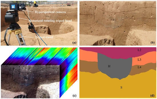
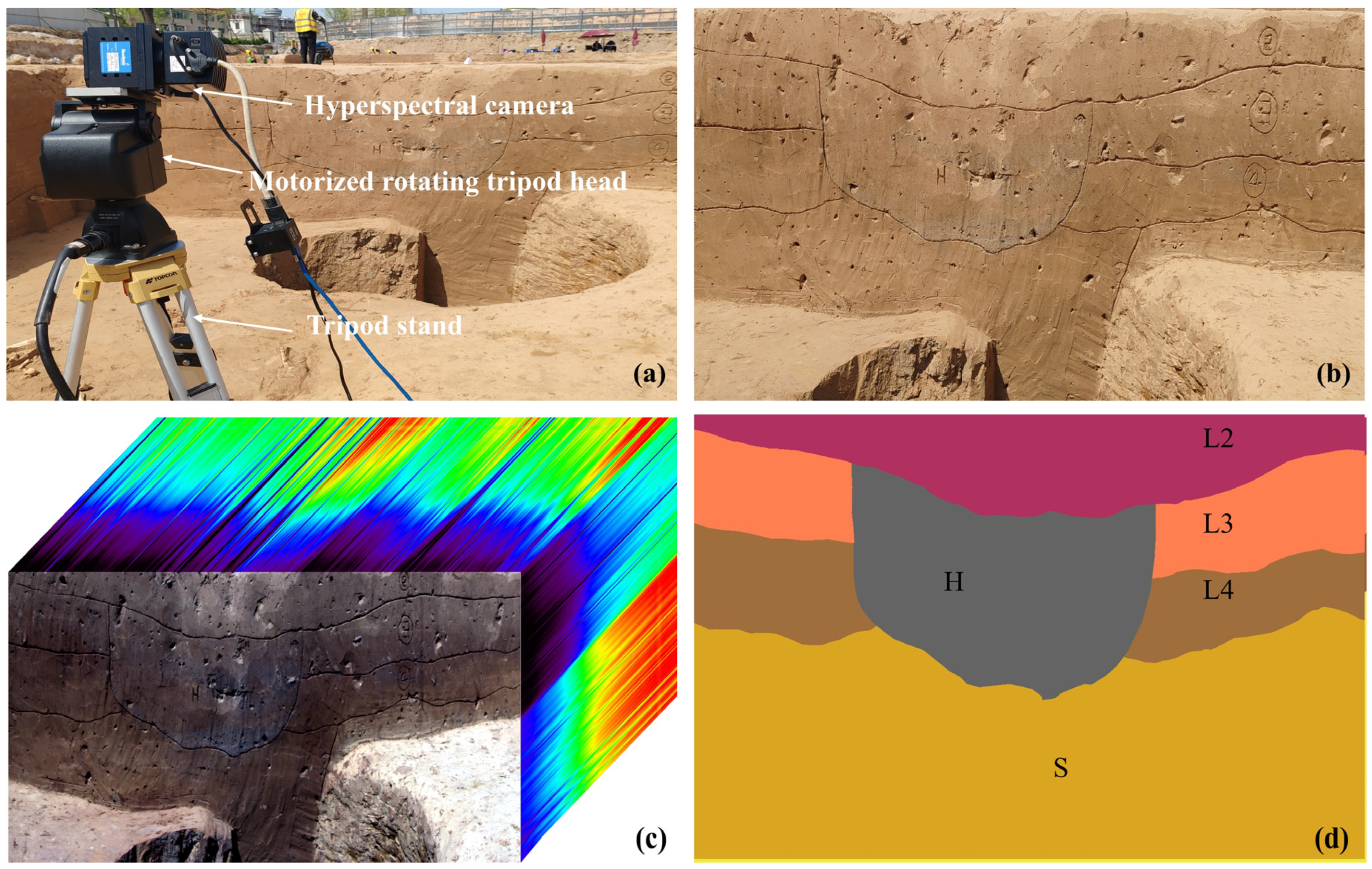
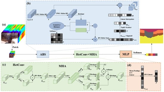
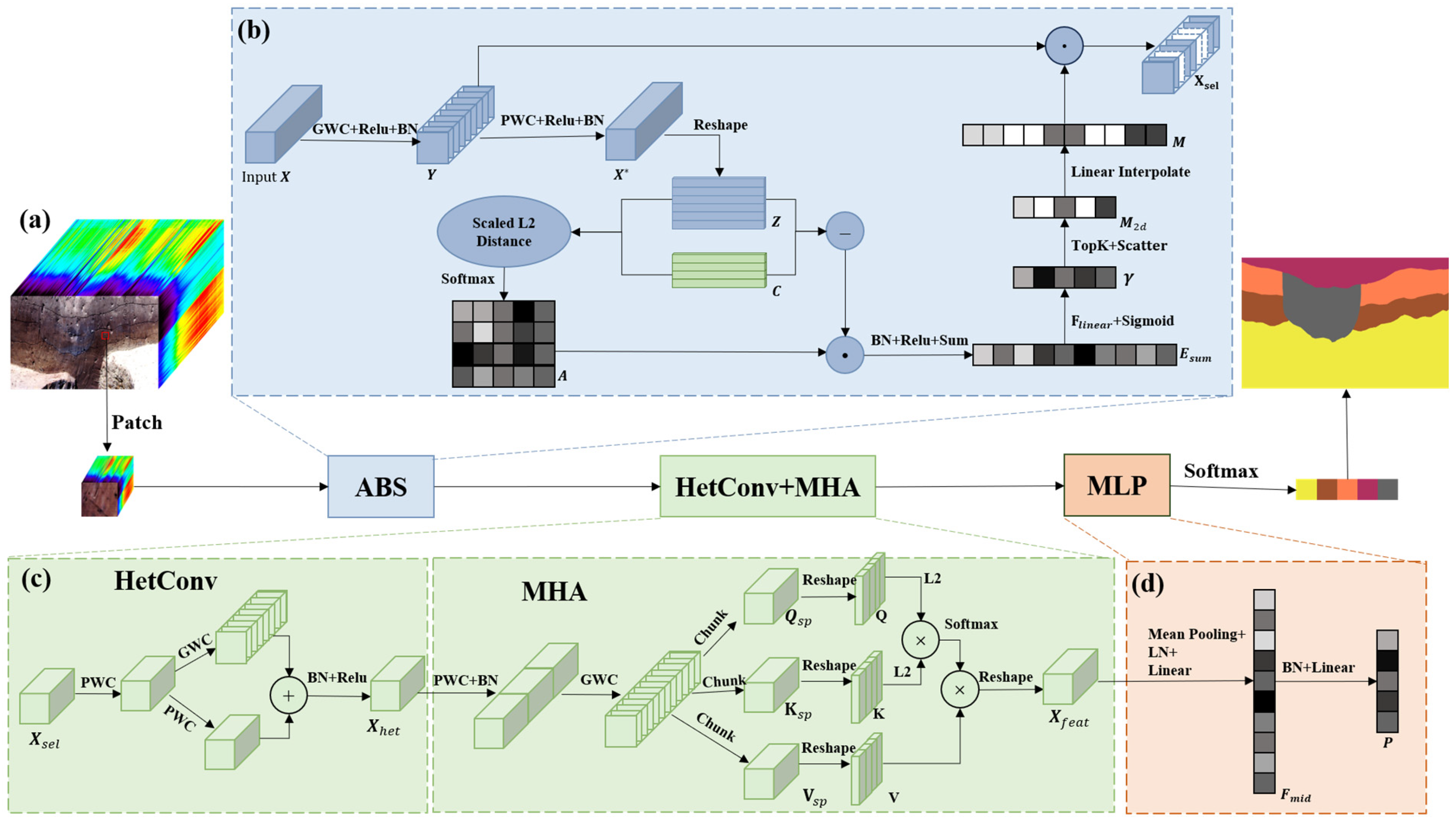
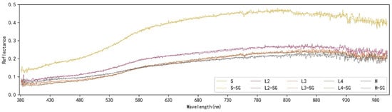
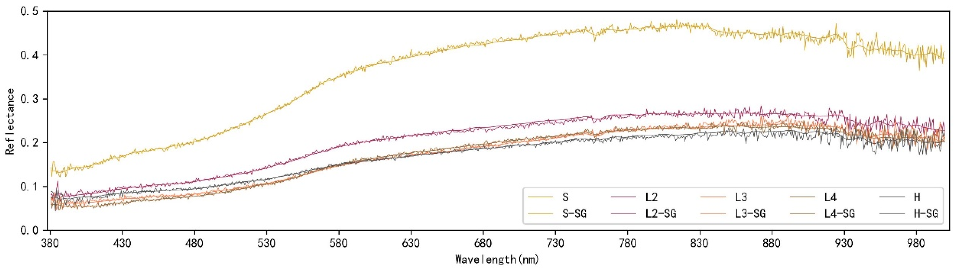
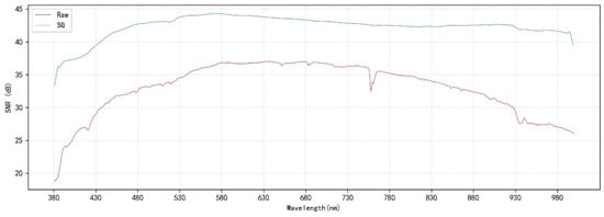
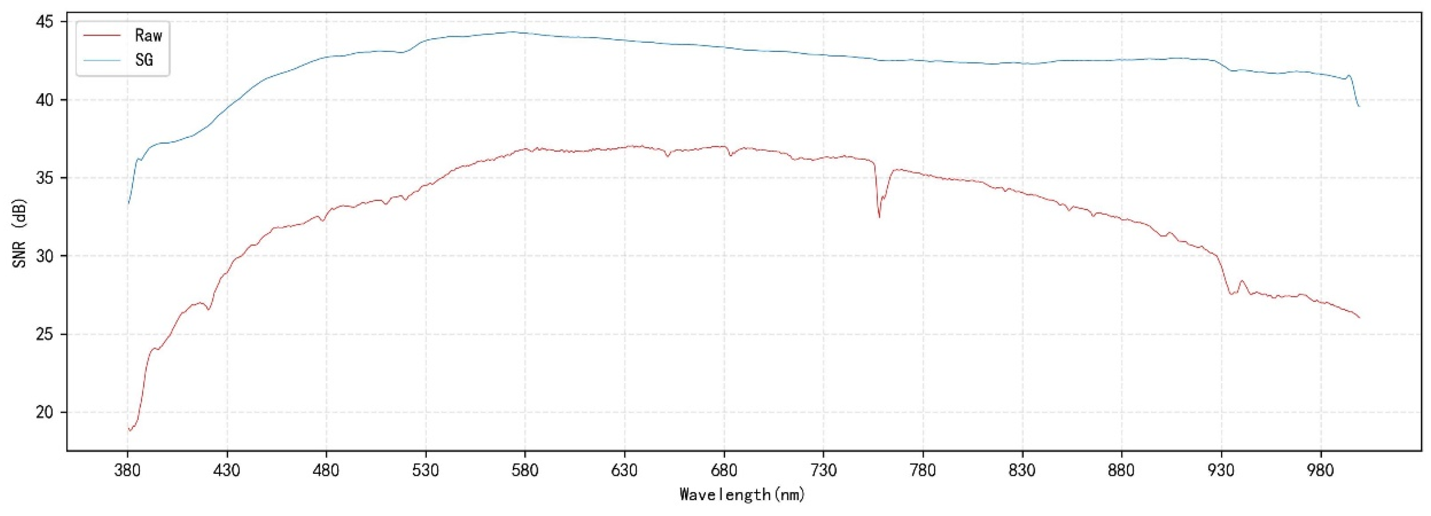
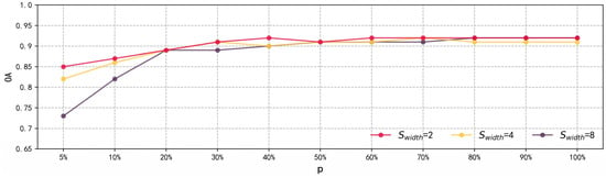
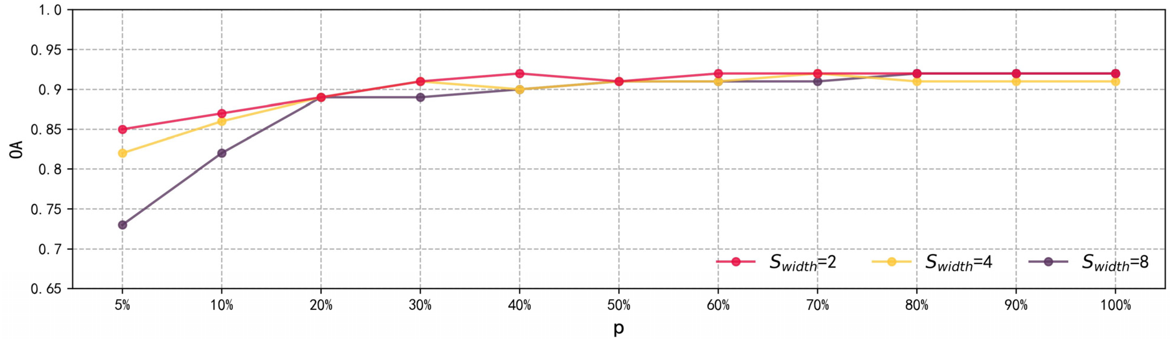
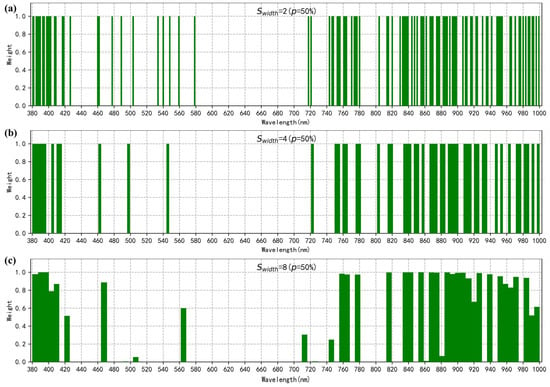
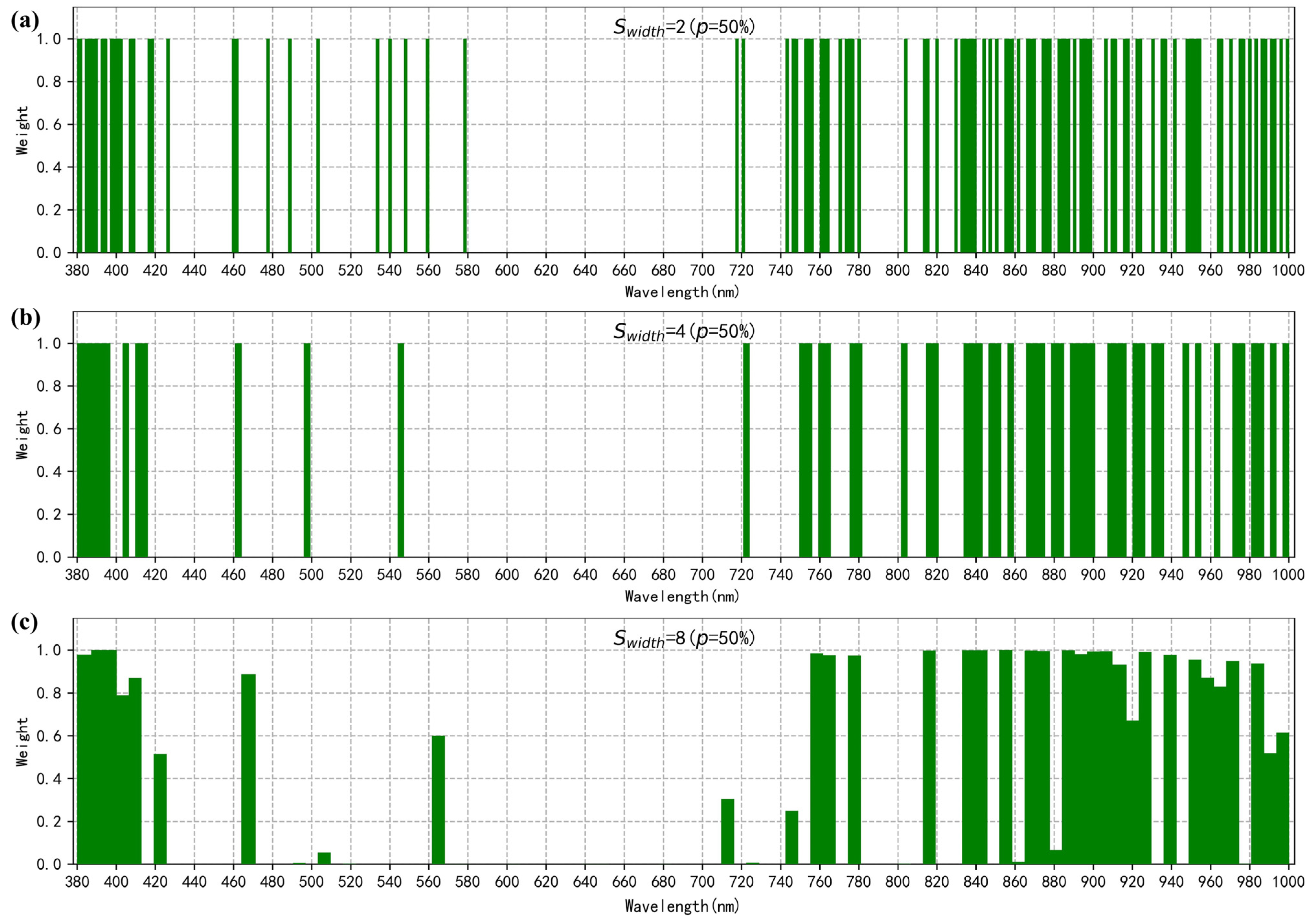
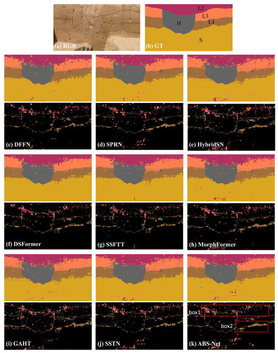
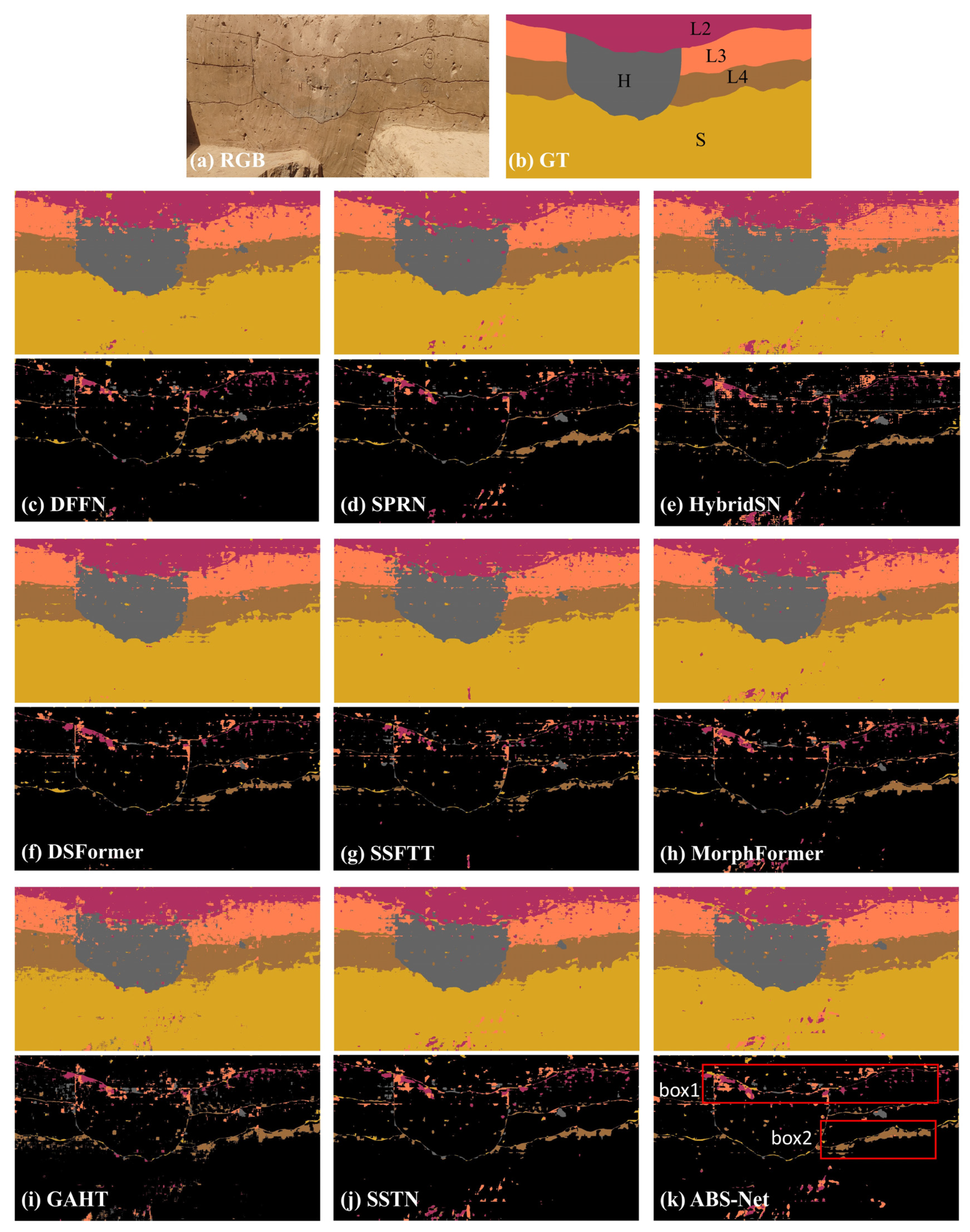
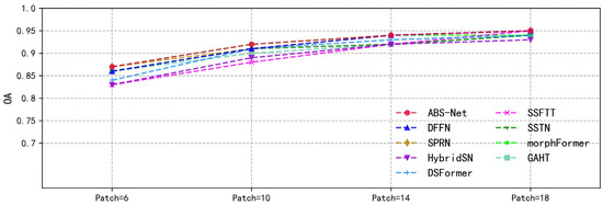
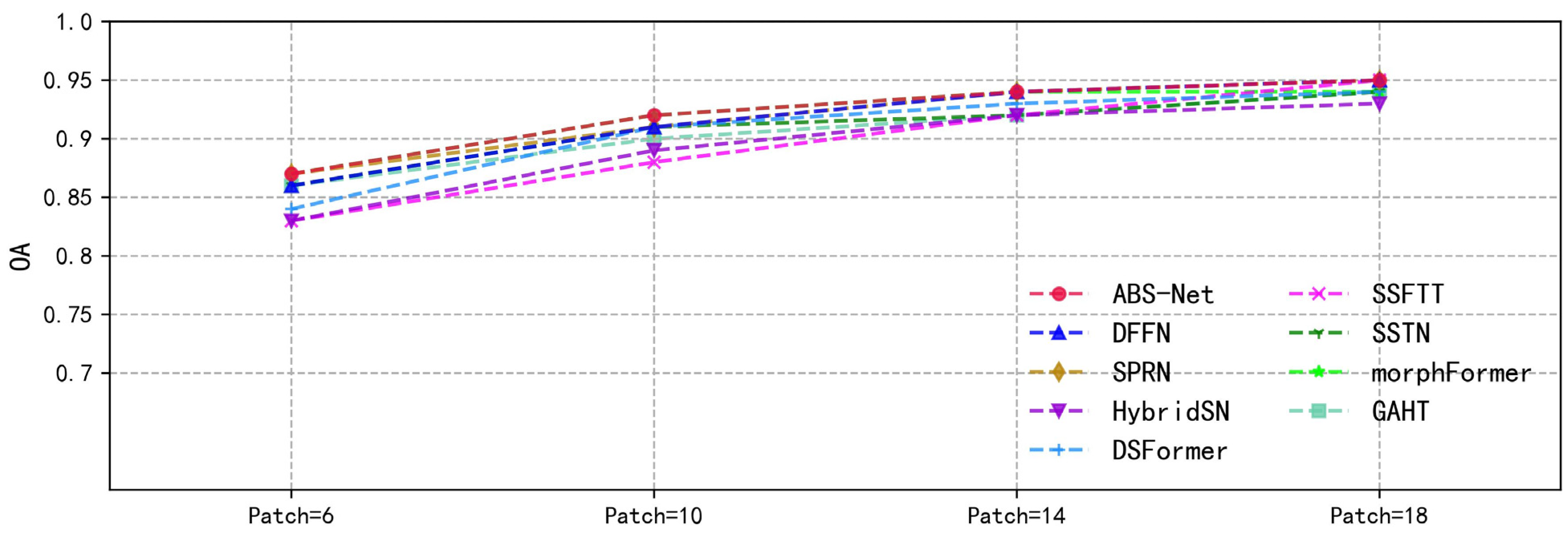

Disclaimer/Publisher’s Note: The statements, opinions and data contained in all publications are solely those of the individual author(s) and contributor(s) and not of MDPI and/or the editor(s). MDPI and/or the editor(s) disclaim responsibility for any injury to people or property resulting from any ideas, methods, instructions or products referred to in the content. |
© 2026 by the authors. Licensee MDPI, Basel, Switzerland. This article is an open access article distributed under the terms and conditions of the Creative Commons Attribution (CC BY) license.