Unsupervised Progressive Domain Adaptation for Underwater Hyperspectral Target Detection Across Increasing Turbidity Levels

Highlights

What are the main findings?

• CTP-DA improved cross-turbidity target–background ranking, while RG-OBS reduced expanded background responses after adaptation. Comparisons with conventional and learning-based detectors, together with matched internal interventions, characterized their complementary roles.

What are the implications of the main findings?

• Combining ordered adaptation with spatial response calibration offers a way to maintain target-specific detection without explicitly estimating water optical parameters.

Abstract

Detecting submerged objects becomes difficult when suspended particles alter spectral signatures and reduce target–background contrast. A detector trained in clear water can consequently lose discrimination and produce extensive background responses as turbidity increases. Here, we present a target-specific framework that couples progressive domain adaptation with object-level response calibration. A nonlinear unmixing autoencoder first learns the target representation from labeled clear-water observations. Cross-turbidity progressive domain adaptation (CTP-DA) then transfers model states, target prototypes, and prediction memory through ordered unlabeled domains. Risk-gated object-level background suppression (RG-OBS) subsequently limits background activation while protecting supported target regions. Across the L1–L5 target domains of the controlled brick-and-stone benchmark, the framework achieved an average precision of 0.9282. This exceeded the strongest external comparator evaluated here by 7.10 percentage points. Ablation experiments linked the ranking improvement to progressive adaptation and the reduction in background response to subsequent spatial calibration. Together, these findings support combining intermediate unlabeled domains with spatial target evidence to sustain underwater detection across controlled turbidity changes.

1. Introduction

Foreign objects such as bricks, stones, and construction debris can obstruct urban drainage pipelines. Conventional closed-circuit television inspection is sensitive to water conditions, illumination, and visibility [1]. Hyperspectral imaging provides spatial structure and narrow-band spectral responses that may distinguish submerged materials from their surroundings. Its feasibility in sewers has also been studied for non-contact pollution monitoring [2].

Turbid water changes more than overall brightness. Wavelength-dependent attenuation and distinct transmission and backscattering processes can alter spectral shape and target–background contrast [3]. Conventional detectors use target similarity, background statistics, or subspace structure. Examples include spectral angle mapper (SAM) [4], constrained energy minimization (CEM) [5], adaptive cosine estimator (ACE) [6], matched filter (MF) [7], and orthogonal subspace projection (OSP) [8]. Their performance can decline when the source target spectrum or estimated background no longer represents the turbid scene.

Underwater hyperspectral detection has addressed these changes through physical spectral models [9], target- and depth-constrained band selection [10,11], and joint depth estimation and detection [12]. TUTDF uses depth-dependent synthetic source domains to reduce synthetic-to-real mismatch [13]. Autoencoder-based unmixing connects reconstruction with abundance estimation [14]. UTD-Net incorporates target priors [15]; NUN-UTD adds prior-preserving and pseudo-mixture constraints with nonlinear decoding [16]. HUTDNet jointly estimates endmembers, abundances, and spectral features [17], whereas NCSS-Net combines target-prior unmixing, self-supervised band selection, and negative-correlation constraints [18]. These approaches motivate target-prior detection, but continual updating across an ordered turbidity sequence requires additional control of response drift.

Progressive domain adaptation decomposes a large shift into successive transitions using intermediate domains [19,20]. In related hyperspectral work, TASR updates target references at test time [21], ICLTD addresses multitemporal spectral variation through contrastive learning [22], and SPADA uses prototypes and stage-wise training for cross-scene classification [23]. SPADA may query target annotations in later stages, so its supervision differs from the present setting. Here, target-domain updating uses unlabeled cubes of the same physical entity, with all L1–L5 masks reserved for evaluation.

Representation adaptation alone does not constrain the extent of connected background responses. Spatial–spectral background suppression [24], adaptive background endmembers [25], and self-supervised background learning [26] address related interference. Recent underwater vision also examines joint image enhancement and captioning [27] and region-aware captioning with foundation-model-derived foreground and background information [28]. These image-to-text studies provide related context for degraded-image representation and regional perception. The present task instead produces target-specific pixel scores from hyperspectral cubes, without language supervision or caption generation.

We address these coupled difficulties by combining CTP-DA, which adapts target–background ranking across turbidity levels, with RG-OBS, which constrains spatial background activation after adaptation.

The main contributions of this study are as follows:

• We construct a controlled underwater hyperspectral cross-turbidity dataset. The primary cross-turbidity benchmark contains 78 hyperspectral cubes collected from 13 physical targets under six increasing relative turbidity levels, L0–L5. L0 is the labeled source domain, whereas L1–L5 are unlabeled target domains introduced in a prescribed order. Their masks are used only for offline evaluation after complete inference. Additional wooden-target and altered-illumination acquisitions extend the full evaluated inventory to 108 cubes across 18 condition-specific sequences (Section 4.6).
• We propose CTP-DA based on a target-prior nonlinear unmixing autoencoder. The method transfers model states, dynamic target prototypes, and unlabeled prediction memory along the prescribed turbidity order and progressively updates the continuous detection response using multi-evidence response fusion, high-confidence pseudo-anchors, and a teacher–student consistency constraint.
• We propose RG-OBS as a response-calibration module independent of cross-stage parameter updates. The module assesses background-response expansion risk from the area and connectivity of the continuous response and applies soft suppression with target-core and boundary protection using multiple sources of target support and candidate connected objects. When the risk is low or no reliable candidate object is obtained, the original CTP-DA response is retained.

2. Dataset Construction and Problem Formulation

2.1. Experimental Environment and Target Materials

We constructed a controlled scene resembling a drainage pipeline to examine how turbidity affects hyperspectral target detection. The acquisition system comprised a transparent acrylic tank, a halogen lamp, and a hyperspectral imager within a dark room enclosed by blackout curtains. The lamp illuminated the tank at approximately 45° to the horizontal plane. During push-broom acquisition, a linear translation stage moved the tank while the imager and lamp remained stationary. Maintaining the imaging geometry within each sequence allowed the turbidity gradient to be examined under comparable viewing conditions.

Six bricks and seven stones represented the solid foreign objects considered in this study. Each specimen was imaged individually on the tank bottom, with magnetic positioning maintaining its location across the six relative turbidity levels, L0–L5. The six cubes acquired for one physical target formed a paired cross-turbidity sequence. The resulting benchmark comprised 13 sequences and 78 hyperspectral cubes, allowing each target to be followed as water conditions changed.

The material evaluation also included three wooden specimens, branch1–branch3, each imaged through L0–L5 under the original illumination. Illumination variation was examined using brick1 alone. The lamp head was rotated 45° left (light1) or right (light2) relative to its original orientation, without moving the lamp mount, imager, or target. Each orientation remained fixed throughout L0–L5. All acquisitions followed the same acquisition and processing protocol. The evaluated inventory therefore comprised 16 physical targets, 18 condition-specific sequences, and 108 cubes. Primary comparisons and ablations used the 13-target benchmark; the material and illumination evaluations are reported in Section 4.6.

2.2. Turbidity Design and Data Acquisition

Kaolin was used to produce a repeatable gradient of particle-induced turbidity. Its weighed additions provided control over suspended scattering particles, avoiding the variable composition of natural sediment and the predominantly absorptive effect of ink.

The tank measured 60 × 20 cm and contained approximately 10 L of water at a depth of 8.5 cm. Successive kaolin additions generated clear-water L0 and five increasingly turbid conditions, L1–L5 (Table 1). These mass-defined levels describe the experimental gradient rather than calibrated turbidity units or the full composition of wastewater.

Table 1. Relative L0–L5 turbidity levels, cumulative kaolin addition, and domain roles in the primary benchmark.

Level	Cumulative Kaolin Mass (g)	Added at This Stage (g)	Nominal Concentration (g L−1)	Domain Role	Cubes
L0	0	0	0	Labeled source	13
L1	0.5	0.5	0.05	Unlabeled target	13
L2	1	0.5	0.10	Unlabeled target	13
L3	2	1	0.20	Unlabeled target	13
L4	4	2	0.40	Unlabeled target	13
L5	5	1	0.50	Unlabeled target	13

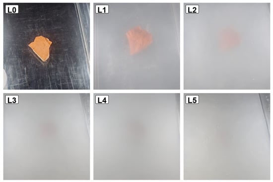
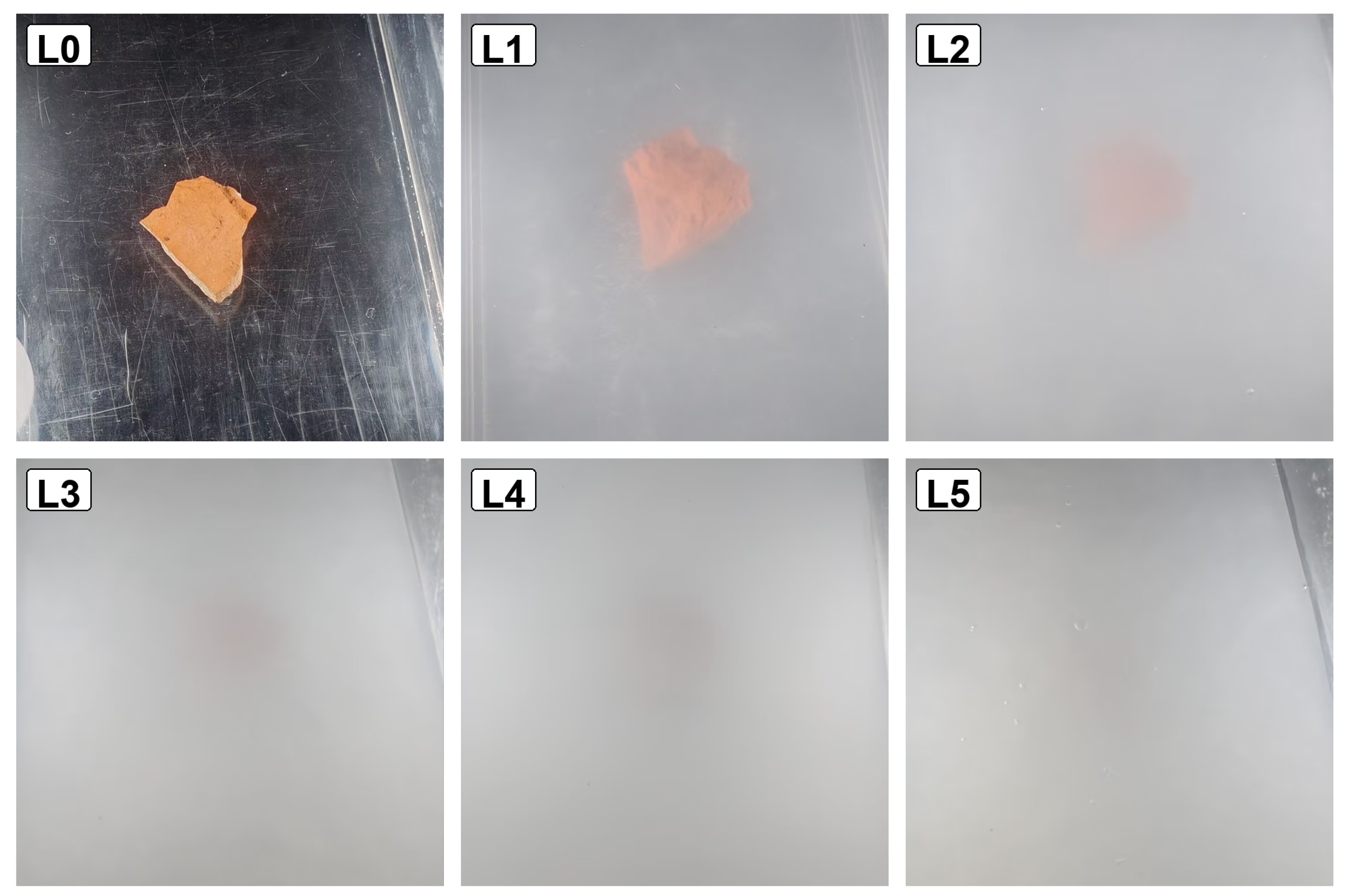
The water was stirred before each acquisition to reduce variation caused by particle settling. Figure 1 documents the resulting visibility changes with RGB reference photographs, which were not used as model inputs.

Figure 1. RGB reference photographs of brick1 at relative turbidity levels L0–L5.

Spectronon Pro was used for focusing, white-panel signal checks, and acquisition control. Each push-broom scan recorded 1000 lines and was stored in BIL format with an associated HDR header.

The raw cubes contained $1000\times 1600$ pixels and 462 spectral bands spanning 388.31–1005.85 nm. Acquisition used a frame rate of 20 frames ${\mathrm{s}}^{-1}$, an integration time of 49.0 ms, and a gain of 0 dB. Sample/Spectral/Line binning was set to 1/2/1 throughout the measurements.

2.3. Data Correction and Preprocessing

Radiometric correction combined dark-field subtraction with the imager calibration files to convert raw digital numbers into radiance. Each radiance cube was then normalized by the mean white-panel spectrum measured at the corresponding turbidity level. The resulting panel-referenced relative reflectance provided a common radiometric basis for comparing target responses across the sequence.

A common $800\times 800$-pixel region was extracted from each $1000\times 1600$-pixel cube, beginning at $x_{\mathrm{start}}=600$ and $y_{\mathrm{start}}=100$. Keeping this window fixed across L0–L5 preserved the spatial correspondence required for sequence-level evaluation.

Pronounced noise at the spectral extremes motivated removal of the corresponding bands. We retained software-indexed bands 50–230, covering 452.83–692.14 nm, to obtain 181 consecutive spectral channels. Combined with the spatial crop, this selection yielded $800\times 800\times 181$ inputs for detection.

2.4. Dataset Annotation and Evaluation Protocol

Reference masks were delineated as polygonal regions on the clear-water L0 images in ENVI 5.6, where target outlines were most visible. Magnetic positioning and the fixed crop supported direct transfer of these masks to L1–L5, without additional registration or boundary redrawing. The selected object was labeled as target and all remaining pixels as background. This common geometric reference allowed changes in detection response to be evaluated as turbidity increased.

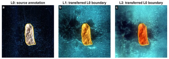
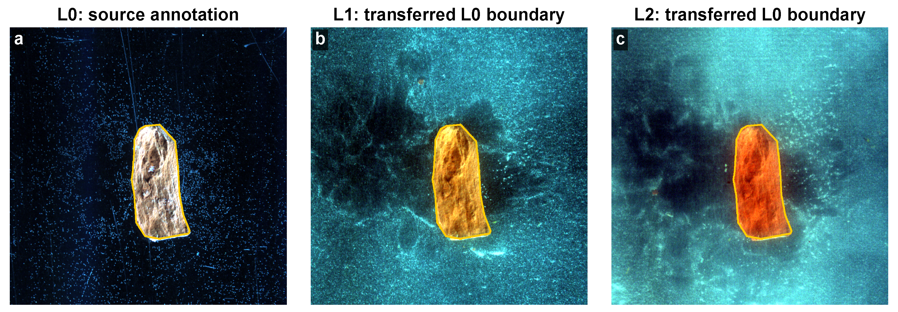
We assessed the spatial correspondence with a boundary-support diagnostic using Gaussian-smoothed Sobel gradients from 12 evenly sampled bands in L1–L2. Searching translations within $\pm 12$ pixels gave a median estimated displacement of 4.1 pixels across 26 target-level pairs; the 95th percentile was 10.9 pixels. Figure 2 illustrates brick4. These gradient-support shifts are not independently measured registration residuals and were not used to modify masks or fit the detector.

Figure 2. L0 reference contours for brick4 across L0–L2: (a) source annotation at L0; (b) L0 reference contour transferred to L1; (c) L0 reference contour transferred to L2. Estimated boundary-support displacements at L1 and L2 were 3.2 and 5.1 pixels, respectively.

Target-domain masks were reserved for offline evaluation. Their transfer from L0 prevented target-label use during adaptation but did not provide independent target-domain annotations. Boundary metrics therefore quantify consistency with the transferred reference and remain subject to its spatial uncertainty.

2.5. Problem Formulation for Target Detection

Let $n\in \{1,\dots ,13\}$ denote a physical-target sequence, and let $l\in \{0,\dots ,5\}$ denote a relative turbidity level. The hyperspectral cube of sequence n at level l is defined as

$$X_l^{\left(n\right)}\in {\mathbb{R}}^{H\times W\times B}.$$

(1)

where $H=W=800$ and $B=181$. Each physical-target sequence has an independently fitted detector, with labeled clear-water L0 followed by unlabeled L1–L5 in cumulative-kaolin order. Pixels are not randomly divided into training, validation, and test sets.

L0 and its mask provide supervised training, target/background median spectra, target area, and the fixed 181-dimensional target prior. The prior initializes the target endmember and supplies prior-target similarity at each stage. L1–L5 masks enter only offline evaluation and visualization after the complete sequence; they do not enter losses, pseudo-anchor selection, model updates, response computation, or threshold selection.

The pixel-level continuous target response produced by the model in target domain l is defined over the range

$$S_l^{\left(n\right)}\in {[0,1]}^{H\times W}.$$

(2)

Higher scores indicate stronger target support. Detection is binary and target-specific, using a prior spectrum; bricks and stones are evaluated as targets, rather than separate recognition classes.

3. Proposed Method

3.1. Overall Framework

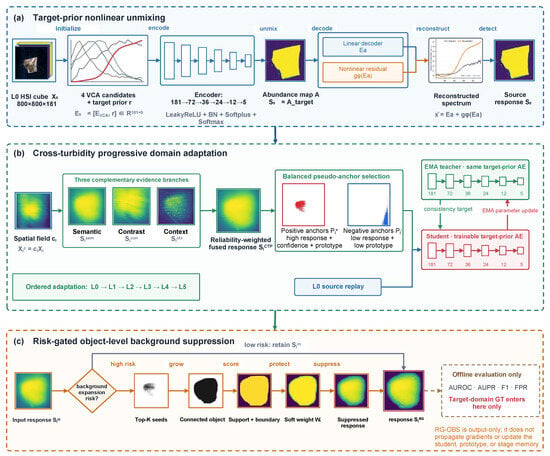
Using the sequence notation in Section 2.5, let $G_0$ denote the L0 mask and r the fixed prior target spectrum. Figure 3 shows the detector architecture and progressive processing.

Figure 3. Framework comprising (a) target-prior-guided nonlinear unmixing and labeled L0 source learning, (b) ordered unlabeled cross-turbidity progressive domain adaptation (CTP-DA), and (c) output-only risk-gated object-level background suppression (RG-OBS). Blue, green, and orange dashed outlines distinguish the three modules, respectively. Arrows indicate data flow and parameter updates as labeled. Target-domain masks are used only for offline evaluation.

As shown in Figure 3, the framework combines labeled L0 representation learning, ordered CTP-DA and output-only RG-OBS. Algorithm 1 summarizes the stage updates and conditional calibration. The final RG-OBS response is used for visualization and evaluation; later stages inherit student parameters, the prototype and uncalibrated response memory. Saved student snapshots also supply the frozen older teacher from L2 onward.

Algorithm 1 Progressive adaptation and response calibration.

Input: labeled L0 cube $X_0$ and mask $G_0$; fixed prior r; ordered unlabeled cubes $X_1,\dots ,X_5$; known stage/material metadata; fixed settings in Section 4.1.

Output: five stage-response maps $S_{\mathrm{RG}}$.

Notation:$S,C$ abbreviate the uncalibrated response/confidence $S_l^{\mathrm{CTP}},C_l$; $\mathcal{H}$ stores $(S,C)$; p is the prototype; $K^{*}$ denotes the undilated seed core associated with the selected candidate.

1 Train the L0 autoencoder; initialize source statistics, $p=p_0$, $A_0=\left|G_0\right|$ and $\mathcal{H}=⌀$ (Equations (3)–(7)).   2 For  $l=1,\dots ,5$  do   3   Initialize student/EMA teacher from the preceding student; freeze the stage-$(l-2)$ student as older teacher for $l\ge 2$. Prepare spatial-field correction, contrast/PCA features and context model (Section 3.3 and Section 4.1).   4   For  $t=1,2,3$  do   5     Compute semantic/abundance, spectral-contrast and context evidence with stripe handling, reliability fusion, memory and graph propagation, yielding uncalibrated $S,C$ (Equations (13)–(43)).   6     Select equal, disjoint pseudo-anchor classes with history-aware scores, supervision weights and stage fractions (Equations (44)–(49); Section 4.1).   7     Reset Adam; optimize CTP-DA with L0 replay, constraining the decoder and updating EMA after each step (Equations (50)–(52)). Update p from corrected-spectrum medians selected using this round’s pre-training $S,C$ (Equations (53) and (54)).   8   End for   9   Recompute final $S,C$ and support maps; preserve the student, p and $\mathcal{H}\leftarrow (S,C)$ for the next stage. 10   Set $S_{\mathrm{in}}\leftarrow \mathcal{N}\left(S\right)$; at L4–L5 replace it by the core–halo calibrated response only if all Section 3.3 acceptance tests pass. 11   Compute U, $Q_{\mathrm{seed}}(S_{\mathrm{in}},U)$ and $z\left(S_{\mathrm{in}}\right)$ (Equations (55)–(57)); set $Q\leftarrow \mathcal{N}\left(Q_{\mathrm{seed}}\right)$, $S_{\mathrm{RG}}\leftarrow S_{\mathrm{in}}$. 12   If $z=0$: emit $S_{\mathrm{RG}}$ and continue to the next stage. 13   Search fixed thresholds: seed by [high Q OR (high U AND $\mathrm{rank}\left(S_{\mathrm{in}}\right)>0.5$)], falling back to max-Q pixels. Use up to five connected seed components per seed threshold; grow, close/fill holes, reject overgrowth and trim while preserving seed cores; retain the best-scoring $(O,K^{*})$ (Equations (58) and (59)). 14   Final fallback check: if O is absent or $\left|O\right|<0.25A_0$, emit $S_{\mathrm{RG}}$ and continue to the next stage. 15   Apply preset area adjustment; conditionally run SGR at L4–L5. Replace O by its refinement only if seed/connectivity/area checks pass; otherwise retain pre-SGR O (Section 3.4). 16   Build distance-decaying W from final O, with radius limits, protection floors, smoothing and weak-support caps, in the order specified in Section 3.4 (Equation (60)). 17   Apply accepted SGR probabilities; otherwise set $W\left[O\right]\leftarrow 1$, retaining exterior W. Always set $W\left[K^{*}\right]\leftarrow 1$. 18   Set $S_{\mathrm{RG}}\leftarrow \min (S_{\mathrm{in}}\odot W,S_{\mathrm{in}})$ and emit $S_{\mathrm{RG}}$ (Equation (61)). 19 End for 20 Return the five stage-response maps.

Operators and settings follow Section 3.3, Section 3.4 and Section 4.1. Output calibration leaves saved states unchanged. Target masks are used only after the complete sequence for evaluation.

3.2. Target-Prior-Guided Nonlinear Unmixing Autoencoder

We use a target-prior-guided nonlinear unmixing autoencoder as the source detector, following the unmixing formulation in [14,16,29]. With $K_s=4$ candidate scene components and one target component, the encoder maps each pixel spectrum $x\in {\mathbb{R}}^B$ to an abundance vector with $K=K_s+1=5$:

$$a=f_{\theta }\left(x\right)\in {\mathbb{R}}^K.$$

(3)

The fifth abundance channel $a_K$ provides the pixel-level target response. Encoder widths follow $B\to 18K_s\to 9K_s\to 6K_s\to 3K_s\to K$, with Leaky ReLU hidden activations and batch normalization, Softplus, and Softmax at the output. Softmax enforces nonnegative abundances that sum to one, preserving the unmixing interpretation.

The decoder retains an abundance interpretation by combining endmembers according to their estimated weights. A learned nonlinear residual supplements this mixture to represent spectral deviations that the linear combination alone cannot capture.

Vertex component analysis (VCA) extracts four candidate components from the complete L0 cube [30]. These components are not assumed to be pure background endmembers. Concatenating them with the target prior initializes the bias-free decoder, which reconstructs spectra through linear and nonlinear residual branches:

$$E_0=[E^{\mathrm{VCA}},r]\in {\mathbb{R}}^{B\times K}.$$

(4)

$$x_n^{\mathrm{rec}}=E{a}_n+g_{\phi }\left(E{a}_n\right).$$

(5)

Here, E is trainable, whereas the reference spectrum r remains fixed throughout the sequence. Its initialized decoder column is updated at a smaller learning rate and remains nonnegative. The residual function $g_{\phi }$ uses widths $181\to 36\to 72\to 181\to 181$, sigmoid activations after the first three linear layers, and a linear output.

L0 labels supervise the target-abundance channel, while spectral reconstruction and abundance regularization constrain the learned representation. The source objective is

$$L_0={\lambda }_{\sup }{L}_{\mathrm{BBCE}}+{\lambda }_{\mathrm{rec}}^{\mathrm{src}}{L}_{\mathrm{rec}}^{\mathrm{src}}+{\lambda }_{\mathrm{ab}}{L}_{\mathrm{ab}}.$$

(6)

Here, $L_{\mathrm{BBCE}}$ is class-balanced, smoothed binary cross-entropy, and $L_{\mathrm{rec}}^{\mathrm{src}}$ is the source-domain mean-squared error (MSE) averaged over pixels and bands. For each pixel, the population variance is computed across its K abundance components. The abundance regularizer sums this variance-based penalty over N pixels:

$$L_{\mathrm{ab}}={\displaystyle \sum _{n=1}^N}{\log }_{10}\left[{\displaystyle \frac{1}{\mathrm{Var}\left(a_n\right)+\epsilon }}\right].$$

(7)

The loss weights are ${\lambda }_{\sup }=20$, ${\lambda }_{\mathrm{rec}}^{\mathrm{src}}=0.20$, and ${\lambda }_{\mathrm{ab}}={10}^{-5}$. Labels are smoothed to 0.95 and 0.05, with class weights $0.5/N^{+}$ and $0.5/N^{-}$ for equal positive and negative contributions. The resulting student parameters ${\theta }_0^S$ initialize adaptation. L0 also supplies target/background median spectra, the initial prototype $p_0$, and the target area $A_0=\left|G_0\right|$ for the subsequent modules.

3.3. CTP-DA: Cross-Turbidity Progressive Domain Adaptation

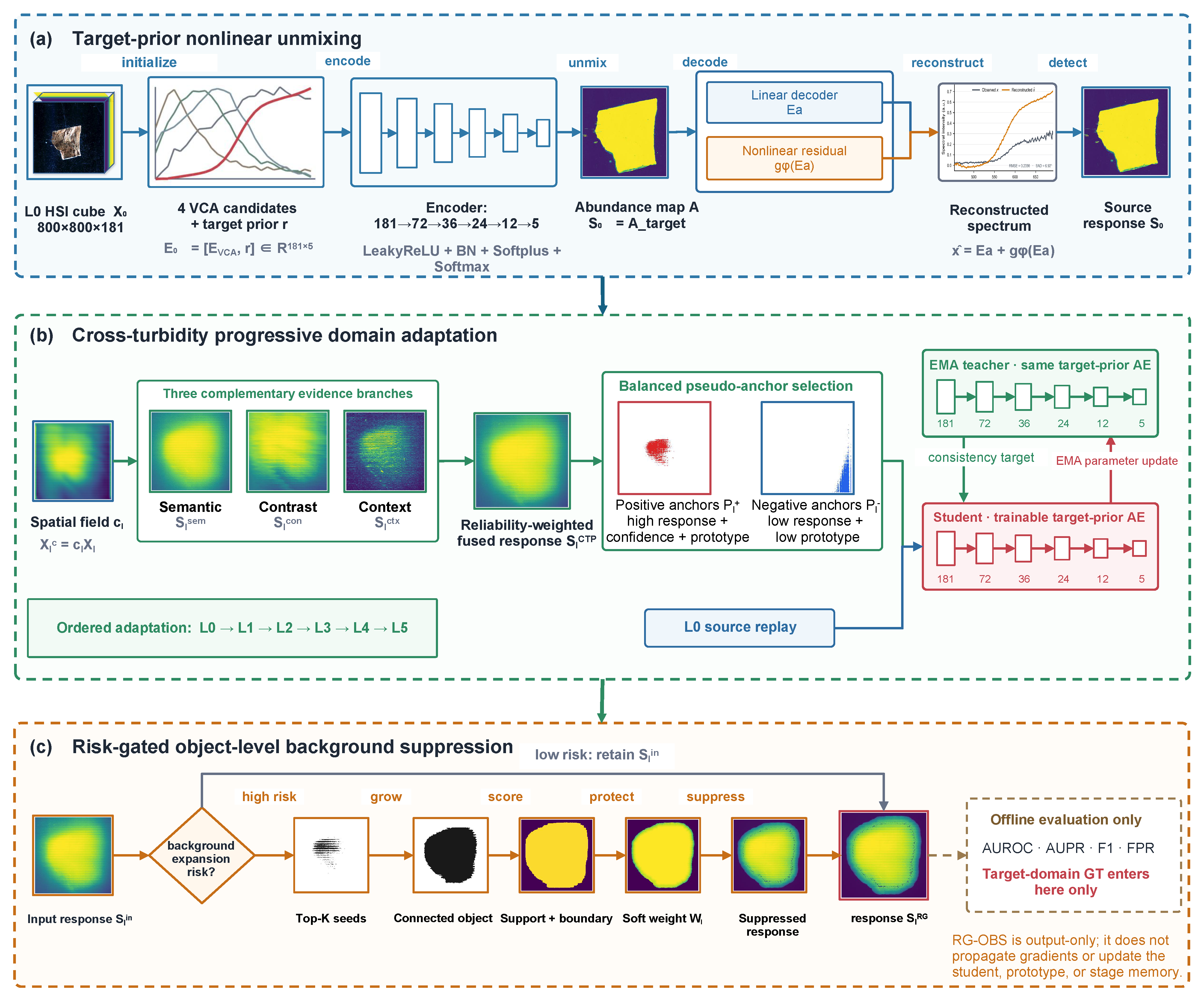
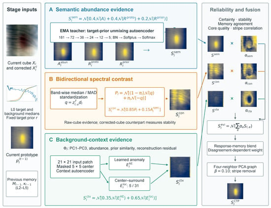
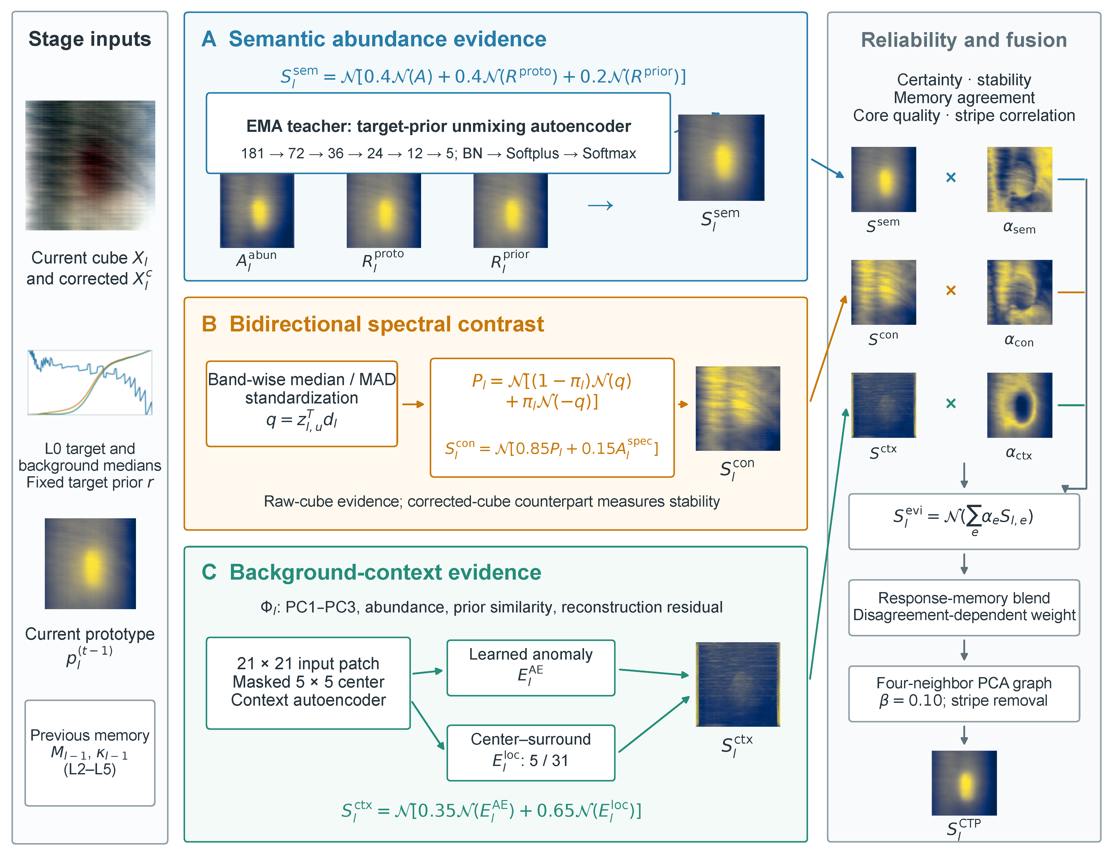
CTP-DA adapts the detector along L0 → L1 $\to \cdots \to$ L5 to accommodate changing spectral contrast and spatial responses. Each stage receives the current cube $X_l$, preceding student parameters ${\theta }_{l-1}^S$, target prototype $p_{l-1}$, and response memory $H_{l-1}$. Three evidence branches construct the stage response, which then guides pseudo-anchor selection and teacher–student updates (Figure 4).

Figure 4. Cross-turbidity progressive domain adaptation (CTP-DA): (A) semantic abundance evidence; (B) bidirectional spectral contrast; and (C) background-context evidence. Blue, orange, and green distinguish the three evidence branches, respectively. Arrows indicate evidence flow through branch construction, reliability-weighted fusion, response-memory blending, and principal component analysis (PCA) graph propagation to produce $S_l^{\mathrm{CTP}}$.

Spatial intensity correction first addresses slowly varying brightness and scan-line fluctuations. Throughout this section, the robust normalization operator is

$${\mathcal{N}}_{a,b}\left(Y\right)=\mathrm{clip}\left({\displaystyle \frac{Y-q_a\left(Y\right)}{q_b\left(Y\right)-q_a\left(Y\right)+\epsilon }},0,1\right).$$

(8)

Here, $q_a$ and $q_b$ are image-wide percentiles, and $\mathcal{N}$ abbreviates ${\mathcal{N}}_{0.5,99.5}$. If the percentile range degenerates, the image minimum and maximum replace its endpoints. The field estimator receives the log-band-mean image

$$Z_l(i,j)={\mathcal{N}}_{1,99}\left(\log \left[\epsilon +{\displaystyle \frac{1}{B}}{\displaystyle \sum _{b=1}^B}{X}_l(i,j,b)\right]\right).$$

(9)

The positive constant $\epsilon$ prevents a zero logarithm argument or denominator. The estimator fits a smoothed intensity field $Z_l^{\mathrm{smooth}}$ with total-variation regularization. Its background-fitting mask $B_l^{\mathrm{bg}}$ excludes the highest 8% of initial responses:

$$L_{\mathrm{field}}={\displaystyle \frac{{\sum }_{i,j}{B}_l^{\mathrm{bg}}\left|F_l^{\mathrm{AE}}-Z_l^{\mathrm{smooth}}\right|}{{\sum }_{i,j}{B}_l^{\mathrm{bg}}}}+{\lambda }_{\mathrm{TV}}\mathrm{TV}\left(F_l^{\mathrm{AE}}\right).$$

(10)

The field estimator is fitted on a bilinearly downsampled $256\times 256$ intensity image. Its estimated field is bilinearly upsampled to the original $800\times 800$ size before row-median residual compensation. This compensation gives the empirical field $F_l$. Its clipped exponential defines a positive coefficient applied equally to all bands of each pixel:

$$c_l=\mathrm{clip}\left[\exp (-\gamma F_l),c_{\min },c_{\max }\right].$$

(11)

$$X_l^c(i,j,:)=c_l(i,j)X_l(i,j,:).$$

(12)

On the corrected cube, the exponential moving average (EMA) teacher estimates target abundance $A_l^{\mathrm{abun}}$ and reconstruction residuals using the student’s architecture. Spectral-angle similarities to the fixed prior and current prototype are

$$R_l^{\mathrm{prior}}\left(u\right)=1-{\displaystyle \frac{\mathrm{SAM}(x_{l,u}^c,r)}{\pi }}.$$

(13)

$$R_l^{\mathrm{proto}}\left(u\right)=1-{\displaystyle \frac{\mathrm{SAM}(x_{l,u}^c,p_l^{(t-1)})}{\pi }}.$$

(14)

Here, $t=1,2,3$ indexes adaptation rounds, with the preceding-stage prototype used on entry. These maps and the abundance response form the semantic evidence:

$$S_l^{\mathrm{sem}}=\mathcal{N}\left[0.40\mathcal{N}\left(A_l^{\mathrm{abun}}\right)+0.20\mathcal{N}\left(R_l^{\mathrm{prior}}\right)+0.40\mathcal{N}\left(R_l^{\mathrm{proto}}\right)\right].$$

(15)

A second branch represents bidirectional target–background contrast. The current cube is standardized by its band-wise median and median absolute deviation (MAD), estimated from up to 100,000 uniformly strided pixels. Applying this scale to the L0 target/background median spectra gives ${\mu }_l^t$ and ${\mu }_l^b$. The standardized pixel $z_{l,u}$ is projected along their discriminative direction:

$$d_l={\displaystyle \frac{{\mu }_l^t-{\mu }_l^b}{{\parallel {\mu }_l^t-{\mu }_l^b\parallel }_2+\epsilon }}.$$

(16)

$$P_l\left(u\right)=\mathcal{N}\left[(1-{\pi }_l)\mathcal{N}\left(z_{l,u}^T{d}_l\right)+{\pi }_l\mathcal{N}(-z_{l,u}^T{d}_l)\right].$$

(17)

Equation (17) normalizes the positive and negative projection directions separately before blending; it does not apply positive-part truncation. The negative-polarity weight is

$${\pi }_l=\mathrm{sigmoid}\left[\mathrm{clip}\left({\displaystyle \frac{l-1.5}{0.75}}-{\displaystyle \frac{a_l^{+}-a_l^{-}}{0.003}},-8,8\right)\right].$$

(18)

The affinities $a_l^{+}$ and $a_l^{-}$ are mean cosine similarities to the L0 target median within the highest 1% of the respective directional responses. This weighting allows the preferred polarity to change with turbidity and current spectral evidence. The branch also includes standardized spectral magnitude:

$$A_l^{\mathrm{spec}}\left(u\right)=\mathcal{N}\left(\sqrt{{\displaystyle \frac{1}{B}}\sum _{b=1}^B{z}_{l,u,b}^2}\right).$$

(19)

$$S_l^{\mathrm{con}}\left(u\right)=\mathcal{N}\left[0.85P_l\left(u\right)+0.15A_l^{\mathrm{spec}}\left(u\right)\right].$$

(20)

The active contrast branch is evaluated on the original cube $X_l$. Its counterpart on $X_l^c$ measures correction stability; semantic evidence instead uses $X_l^c$.

Background context provides the third evidence source. Its six-channel feature tensor ${\mathrm{\Phi }}_l$ contains three PCA components: target abundance, prior similarity, and reconstruction residual. A context autoencoder learns masked-center reconstruction from low-response background patches. For each of the six feature channels, the local anomaly takes the absolute difference between $5\times 5$ and $31\times 31$ window means. These absolute differences are averaged across channels and then normalized by $\mathcal{N}$ to obtain $E_l^{\mathrm{loc}}$. It complements the learned reconstruction anomaly:

$$S_l^{\mathrm{ctx}}=\mathcal{N}\left[0.35\mathcal{N}\left(E_l^{\mathrm{AE}}\right)+0.65\mathcal{N}\left(E_l^{\mathrm{loc}}\right)\right].$$

(21)

The context network uses $21\times 21$ patches and Smooth-L1 reconstruction of the masked $5\times 5$ center. It has convolutional widths $6\to 24\to 24\to 12\to 24\to 6$, with GroupNorm and SiLU hidden transformations.

Before fusion, the semantic responses from the corrected and original cubes and both contrast responses undergo directional stripe removal. For a normalized map S, let $h_r$ and $h_c$ be its row- and column-median profiles minus their Gaussian-smoothed profiles. The operation is

$${\mathcal{D}}_{\eta }\left(S\right)(i,j)=\mathcal{N}\left[\mathcal{N}\left(S\right)(i,j)-\eta \{h_r\left(i\right)+h_c\left(j\right)\}\right].$$

(22)

The Gaussian width is 5 pixels; $\eta =1$ before fusion. In the following fusion definitions, branch maps denote these processed responses. Raw-cube semantic and corrected-cube contrast counterparts are denoted by $S_l^{\mathrm{sem},\mathrm{raw}}$ and $S_l^{\mathrm{con},\mathrm{c}}$.

Reliability weighting determines how the three branches contribute at each pixel. For $e\in \{\mathrm{sem},\mathrm{con},\mathrm{ctx}\}$, response certainty is

$$c_e\left(u\right)=2\left|S_{l,e}\left(u\right)-0.5\right|.$$

(23)

Semantic internal agreement additionally compares the three normalized constituent maps $V_l=\{\mathcal{N}\left(A_l^{\mathrm{abun}}\right),\mathcal{N}\left(R_l^{\mathrm{proto}}\right),\mathcal{N}\left(R_l^{\mathrm{prior}}\right)\}$:

$$I_l\left(u\right)=\mathrm{clip}\left[1-\underset{V\in V_l}{\max }V\left(u\right)+\underset{V\in V_l}{\min }V\left(u\right),0,1\right].$$

(24)

$${\tilde{c}}_e=\left\{\begin{array}{cc}\mathcal{N}\left(c_e{I}_l\right),\hfill & e=\mathrm{sem},\hfill \\ \mathcal{N}\left(c_e\right),\hfill & e\in \{\mathrm{con},\mathrm{ctx}\}.\hfill \end{array}\right.$$

(25)

The stability term compares responses before and after correction, or the learned and local context cues:

$$v_e=\left\{\begin{array}{cc}1-|S_l^{\mathrm{sem}}-S_l^{\mathrm{sem},\mathrm{raw}}|,\hfill & e=\mathrm{sem},\hfill \\ 1-|S_l^{\mathrm{con}}-S_l^{\mathrm{con},\mathrm{c}}|,\hfill & e=\mathrm{con},\hfill \\ 1-|\mathcal{N}\left(E_l^{\mathrm{AE}}\right)-\mathcal{N}\left(E_l^{\mathrm{loc}}\right)|,\hfill & e=\mathrm{ctx}.\hfill \end{array}\right.$$

(26)

Historical memory $H_{l-1}$ stores the preceding uncalibrated response $M_{l-1}$ and confidence ${\kappa }_{l-1}$. Memory scores are normalized by $\mathcal{N}$ when read. The temporal agreement is

$$t_e=\left\{\begin{array}{cc}1,\hfill & l=1,\hfill \\ 1-|S_{l,e}-M_{l-1}|,\hfill & l\ge 2.\hfill \end{array}\right.$$

(27)

Global quality factors use nonnegative response–memory correlations $h_e$, response–stripe correlations $b_e$, and mean map values, denoted by angle brackets. Correlations are Pearson correlations after robust scaling, evaluated on up to approximately 50,000 uniformly strided pixels; a degenerate map gives zero. The stripe map is the normalized mean absolute row/column high-frequency field of the three PCA channels. For the highest 5% response core, quality is the largest-component fraction minus the fraction of core pixels on the image edges. Semantic core reliability $k_{\mathrm{sem}}$ linearly maps this quality from [0.80,0.92] into [0,1], with clipping. The global factors are

$$\begin{array}{c}{g}_{\mathrm{sem}}=\mathrm{clip}[0.15+0.25h_{\mathrm{sem}}+0.15⟨I_l⟩+0.10⟨v_{\mathrm{sem}}⟩+0.45k_{\mathrm{sem}}\hfill \\ +0.20\max \{0,(3-l)/2\}⟨I_l⟩-0.20b_{\mathrm{sem}},0.05,1].\hfill \end{array}$$

(28)

$$\begin{array}{c}{g}_{\mathrm{con}}=\mathrm{clip}[0.20+0.40h_{\mathrm{con}}+0.15|2{\pi }_l-1|+0.10⟨v_{\mathrm{con}}⟩\hfill \\ +0.20(1-⟨I_l⟩)-0.25b_{\mathrm{con}},0.05,1].\hfill \end{array}$$

(29)

$$g_{\mathrm{ctx}}=\mathrm{clip}\left[0.03+0.25h_{\mathrm{ctx}}+0.20h_{\mathrm{AE},\mathrm{loc}}+0.10⟨v_{\mathrm{ctx}}⟩-0.40b_{\mathrm{ctx}},0.01,0.08\right].$$

(30)

Here, $h_{\mathrm{AE},\mathrm{loc}}$ is the nonnegative correlation between learned and local context anomalies, and $h_e=0$ at L1. If semantic–contrast correlation is at most $-0.25$ and their core qualities differ by at least 0.35, the lower-quality branch’s global factor is multiplied by 0.20. This veto limits strongly conflicting evidence. The implemented reliability and normalized fusion are

$$\begin{array}{c}{r}_e\left(u\right)=\mathrm{clip}\{g_e^4[0.25+0.75{\tilde{c}}_e\left(u\right)][0.45+0.55v_e\left(u\right)]\hfill \\ \times [0.45+0.55t_e\left(u\right)],{10}^{-4},1\}.\hfill \end{array}$$

(31)

$${\alpha }_e\left(u\right)={\displaystyle \frac{r_e\left(u\right)}{{\sum }_k{r}_k\left(u\right)+{10}^{-6}}}.$$

(32)

With the implemented context cap, $0.{08}^4<{10}^{-4}$, so the enabled context branch has $r_{\mathrm{ctx}}={10}^{-4}$. Its normalized weight still varies with the other branches. Context supplies floor-weighted auxiliary evidence and contributes to inter-branch disagreement; its raw reliability is not independently modulated under these presets.

$$S_l^{\mathrm{evi}}\left(u\right)=\mathcal{N}\left[\sum _e{\alpha }_e\left(u\right)S_{l,e}\left(u\right)\right].$$

(33)

The fused confidence uses response certainty $c_e$, rather than the internal-agreement-adjusted ${\tilde{c}}_e$, together with mean response and normalized disagreement:

$${\overline{S}}_l={\displaystyle \frac{1}{3}}\sum _e{S}_{l,e}.$$

(34)

$$D_l={\mathcal{N}}_{0,99.5}\left[{\displaystyle \frac{1}{3}}\sum _e|S_{l,e}-{\overline{S}}_l|\right].$$

(35)

$$C_l^{\mathrm{evi}}=\mathrm{clip}\left[(1-D_l)\sum _e{\alpha }_e{c}_e,0,1\right].$$

(36)

At L1, no response memory is available and $m_l=0$. From L2 onward, historical confidence, branch disagreement, and historical response certainty determine the memory weight:

$$\begin{array}{c}{m}_l\left(u\right)=\mathrm{clip}\{0.90[0.35+0.65{\kappa }_{l-1}\left(u\right)][0.75+0.25D_l\left(u\right)]\hfill \\ \times [0.5+|M_{l-1}\left(u\right)-0.5\left|\right],0,0.90\}.\hfill \end{array}$$

(37)

$$S_l^{\mathrm{mem}}=\mathcal{N}\left[(1-m_l)S_l^{\mathrm{evi}}+m_l{M}_{l-1}\right].$$

(38)

$$C_l^{\mathrm{mem}}=\mathrm{clip}\left[(1-m_l)C_l^{\mathrm{evi}}+m_l{\kappa }_{l-1},0,1\right].$$

(39)

The memory response then undergoes one four-neighbor graph-propagation step. Let $f_u$ denote the three normalized PCA features after row/column stripe removal, and $b\left(u\right)$ their stripe map. For adjacent pixels, the edge weight is

$$\begin{array}{c}{w}_{uv}=\exp \left(-{\displaystyle \frac{{\parallel f_u-f_v\parallel }_2^2/3}{0.05}}\right)\hfill \\ \times \exp \left[-2\{\max (b\left(u\right),b\left(v\right))+s_{uv}\}\right]\mathrm{clip}(C_l^{\mathrm{mem}}\left(v\right),0.05,1).\hfill \end{array}$$

(40)

The directional term $s_{uv}$ is the mean absolute row-profile residual divided by each PCA channel’s standard deviation, averaged over channels, for horizontal edges; column profiles are used for vertical edges. Edges crossing the image boundary have zero weight. With self-weight 2, graph propagation is

$$S_l^{\mathrm{graph}}\left(u\right)=\mathcal{N}\left[{\displaystyle \frac{2S_l^{\mathrm{mem}}\left(u\right)+{\sum }_{v\in {\mathcal{N}}_4\left(u\right)}{w}_{uv}{S}_l^{\mathrm{mem}}\left(v\right)}{2+{\sum }_{v\in {\mathcal{N}}_4\left(u\right)}{w}_{uv}}}\right].$$

(41)

$$S_l^{\mathrm{CTP}}={\mathcal{D}}_{0.75}\left(\mathcal{N}\left[(1-\beta )S_l^{\mathrm{mem}}+\beta S_l^{\mathrm{graph}}\right]\right).$$

(42)

Here, $\beta =0.10$. The stripe diagnostic $b_l^{*}$ is the pixel-wise maximum of the PCA, semantic, contrast, and final-response stripe maps. Response stripe maps are the normalized absolute field removed in Equation (22). The final confidence passed to adaptation and memory is

$$C_l=\mathrm{clip}\left[C_l^{\mathrm{mem}}(1-0.5b_l^{*}),0.02,1\right].$$

(43)

For unlabeled adaptation, equal numbers of positive and negative pseudo-anchors are ranked using $S=\mathcal{N}\left(S_l^{\mathrm{CTP}}\right)$, $R=\mathcal{N}\left(R_l^{\mathrm{proto}}\right)$, and confidence $C_l$. Without history, their scores are

$$Q_l^{+}=S{C}_l(0.5+0.5R).$$

(44)

$$Q_l^{-}=(1-S)C_l(1-R).$$

(45)

For L2–L5, temporal agreement is

$$a_l=1-|S-M_{l-1}|.$$

(46)

Historical conflict reduces confidence when $a_l<0.60$ and ${\kappa }_{l-1}\ge 0.60$:

$${\tilde{C}}_l=C_l(0.35+0.65a_l)\left\{\begin{array}{cc}0.5,\hfill & a_l<0.60\mathrm{and}{\kappa }_{l-1}\ge 0.60,\hfill \\ 1,\hfill & \mathrm{otherwise}.\hfill \end{array}\right.$$

(47)

$$Q_l^{+}=S{\tilde{C}}_l(0.5+0.5R)\left[0.5+0.5\{{\kappa }_{l-1}{M}_{l-1}+(1-{\kappa }_{l-1})S\}\right].$$

(48)

$$Q_l^{-}=(1-S){\tilde{C}}_l(1-R)\left[0.5+0.5\{{\kappa }_{l-1}(1-M_{l-1})+(1-{\kappa }_{l-1})(1-S)\}\right].$$

(49)

Positive anchors are selected first; negative anchors exclude all selected positives. Each class uses its stage-dependent top-ranked fraction, with at least 512 pixels and at most half the image. Selected joint scores are clipped to [0.05,1] as supervision weights. The student starts from the preceding-stage parameters and minimizes

$$\begin{array}{c}{L}_{\mathrm{CTP}}=3L_{\mathrm{pseudo}}+8L_{\mathrm{replay}}+2L_{\mathrm{ema}}+0.5L_{\mathrm{old}}\hfill \\ +0.03L_{\mathrm{rec}}^{\mathrm{adapt}}+10L_{\mathrm{prox}}.\hfill \end{array}$$

(50)

The first two terms are class-balanced, smoothed binary cross-entropy for weighted target pseudo-anchors and labeled L0 replay, respectively. The consistency terms are target-abundance MSE against the current teacher and the earlier-stage teacher; the latter is active from L2 onward. Proximity regularization averages squared parameter deviations from stage initialization. Unlike the pure source MSE in Section 3.2, the adaptation reconstruction term includes the implemented scale and source replay:

$$L_{\mathrm{rec}}^{\mathrm{adapt}}=10\left[\mathrm{MSE}(X_l^{c,\mathcal{B}},{\widehat{X}}_l^{c,\mathcal{B}})+0.25\mathrm{MSE}(X_0^{\mathcal{R}},{\widehat{X}}_0^{\mathcal{R}})\right].$$

(51)

Here, $\mathcal{B}$ and $\mathcal{R}$ denote target-anchor and source-replay mini-batches; each MSE is averaged over spectra and bands. Thus, the effective MSE coefficients in the adaptation objective are 0.30 and 0.075, respectively. The source reconstruction coefficient remains 0.20.

After each student optimizer update, the teacher is updated by EMA without backpropagation [31]:

$${\theta }_l^T\leftarrow \mu {\theta }_l^T+(1-\mu ){\theta }_l^S.$$

(52)

Prototype updating occurs once after each adaptation round. Let ${\mathcal{I}}_l^{\left(t\right)}$ contain the highest 1% of pixels ranked by normalized response times confidence, with a minimum of 64 pixels. With unit denoting L2 normalization, the corrected-spectrum median gives

$$p_l^{\mathrm{cand},\left(t\right)}=\mathrm{unit}\left[\underset{u\in {\mathcal{I}}_l^{\left(t\right)}}{\mathrm{median}}{x}_{l,u}^c\right].$$

(53)

$$p_l^{\left(t\right)}=\mathrm{unit}\left[\rho \mathrm{unit}\left(p_l^{(t-1)}\right)+(1-\rho )p_l^{\mathrm{cand},\left(t\right)}\right],t=1,2,3.$$

(54)

The current-domain prototype starts from $p_l^{\left(0\right)}=p_{l-1}$, and its final value $p_l^{\left(3\right)}$ becomes $p_l$ for the next stage. The momenta are $\mu =0.995$ and $\rho =0.90$. After three rounds, the final teacher and prototype recompute the stage response and confidence. Student parameters, the final prototype, and uncalibrated response memory pass to the next stage.

For core–halo output calibration at L4–L5, write $S=\mathcal{N}\left(S_l^{\mathrm{CTP}}\right)$ and exclude its upper 3% from background estimation: $M=\mathbf{1}[S<q_{97}\left(S\right)]$, where $q_p$ is the spatial pth percentile. With $G_{60}$ denoting Gaussian smoothing of width 60 pixels and nearest-edge padding,

$$F={\displaystyle \frac{G_{60}\ast \left(SM\right)}{\max (G_{60}\ast M,{10}^{-4})}},\widehat{S}=\mathcal{N}(S-{\beta }_{l}F),({\beta }_4,{\beta }_5)=(0.05,0.20).$$

The candidate $\widehat{S}$ is accepted if its Pearson correlation with S, computed after robust scaling as above, is at least 0.98; its top-5% core quality decreases by at most 0.05; and its median upper-3%-versus-remaining-pixel gap retains at least 0.98 of the original gap. Quality is the largest-component fraction minus the image-edge fraction defined above; each map uses its own quantiles. Otherwise, S is retained. This output-only calibration leaves pseudo-anchors, prototypes, and transferred memory unchanged.

3.4. RG-OBS: Risk-Gated Object-Level Background Suppression

RG-OBS constrains connected background responses after adaptation. Its input $S_l^{\mathrm{in}}$ is the accepted core–halo response at L4–L5, or the normalized uncalibrated response otherwise. Additional inputs are abundance $A_l^{\mathrm{abun}}$, prior/prototype similarities $R_l^{\mathrm{prior}},R_l^{\mathrm{proto}}$, and L0 area $A_0$. Risk diagnosis covers L1–L5; calibration leaves gradients and all states transferred to the next stage unchanged.

We first compute the pixel-percentile rank of each of the three target-support maps and take their pixel-wise maximum to form the integrated target support. This support and the rank of the RG-OBS input response $S_l^{\mathrm{in}}$ jointly define the object-seed score:

$$U_l\left(u\right)=\max \{\mathrm{rank}\left(A_l^{\mathrm{abun}}\right),\mathrm{rank}\left(R_l^{\mathrm{prior}}\right),\mathrm{rank}\left(R_l^{\mathrm{proto}}\right)\},$$

(55)

$$Q_l^{\mathrm{seed}}\left(u\right)=\mathrm{rank}\left(S_l^{\mathrm{in}}\right)[0.5+0.5U_l\left(u\right)].$$

(56)

This construction requires high-response regions to receive abundance or spectral-similarity support, rather than determining target objects from response amplitude alone. Background-response expansion risk is diagnosed using the area ratios of two high-response levels and the largest connected component at a low threshold. The low and high thresholds are used to identify potential large-area response expansion and to determine whether high-confidence background false responses are present, respectively.

$$z_l^{\mathrm{risk}}=1[r_l\left(0.2\right)>{\tau }_{0.2}\vee r_l\left(0.4\right)>{\tau }_{0.4}\vee n_l^{\max }\left(0.2\right)>\kappa A_0].$$

(57)

In Equation (57), $r_l\left(\tau \right)$ is the proportion of pixels whose input response exceeds threshold $\tau$, and $n_l^{\max }\left(0.2\right)$ is the area of the largest connected component in the mask defined by the 0.2 threshold. The parameters ${\tau }_{0.2}$ and ${\tau }_{0.4}$ are the response-area thresholds at the two levels, and $\kappa$ scales the connected-component risk threshold according to the labeled L0 target area $A_0$. The risk gate determines whether RG-OBS enters object search or passes through its input response. The fixed risk values are ${\tau }_{0.2}=0.10$, ${\tau }_{0.4}=0.05$, and $\kappa =5$.

Under high risk, RG-OBS extracts connected cores at multiple high-percentile seed thresholds and performs connected growth, closing, and hole filling within a region jointly constrained by the response and target support. The score of each candidate object combines its regional response, seed strength, target spectral support, consistency with the source-domain object scale, and inner-versus-outer boundary contrast. It also penalizes area mismatch, anomalous expansion, and contact with the image boundary:

$$O_l^{*}=\arg \underset{O}{\max }{J}_l\left(O\right).$$

(58)

$$\begin{array}{c}{J}_l\left(O\right)=0.18{\mu }_S+0.27{\mu }_Q+0.40U_O+0.15C_{\mathrm{area}}\hfill \\ +0.50\mathrm{clip}(C_{\mathrm{bnd}},-0.20,0.20)-P_{\mathrm{obj}}.\hfill \end{array}$$

(59)

In Equation (59), ${\mu }_S$ and ${\mu }_Q$ are the mean input response and mean seed score of the candidate region; $U_O$ is the regional target support; $C_{\mathrm{area}}$ and $C_{\mathrm{bnd}}$ quantify area consistency and inner-versus-outer boundary contrast, respectively; and $P_{\mathrm{obj}}$ summarizes the penalties for area mismatch, anomalous expansion, and boundary contact. The support $U_O$ is the average of the regional mean and 95th-percentile support. Within the allowed area interval, $C_{\mathrm{area}}$ decreases from one according to absolute log area-ratio deviation, normalized by $\log 8$ and clipped to [0,1]. Outside that interval, it is the clipped ratio of candidate area to minimum area, or maximum area to candidate area, respectively. The penalty weights are 0.65 for relative area violation, 0.30 for relative excess above the soft area cap, and 0.10 for image–border contact. Boundary contrast averages the inner-minus-outer mean differences of the input response and integrated target support within a five-pixel band. After candidate generation, overgrowth rejection, and core-preserving trimming, the highest-scoring candidate is retained. A final fallback returns the input response if no candidate is found or the selected area is below $0.25A_0$ (Equation (61)).

Before SGR, undersized objects undergo support-guided growth, whereas oversized objects undergo core-preserving trimming; the source-relative lower/upper triggers are 0.75/4.0 for brick and 0.50/3.0 for stone, with both routes disabled for the generic preset.

For valid candidates at L4 and L5, RG-OBS further refines the object boundary using seeded graph refinement (SGR) based on PCA graph features, foreground/background seeds, and four-neighbor smoothing. If the refined area falls outside the allowed range, the SGR result is discarded and the original candidate is retained. SGR is therefore a conditional boundary-refinement procedure for highly turbid stages, rather than an independent detector.

The final object O defines Euclidean distance $d_O$. The base distance weight is

$$W_l^{\mathrm{base}}\left(u\right)={\kappa }_{\mathrm{out}}+(1-{\kappa }_{\mathrm{out}})\exp \left[-{\displaystyle \frac{d_O^2\left(u\right)}{2{\sigma }_c^2}}\right].$$

(60)

To obtain the effective weight $W_l$, use Equation (60) within support radius R, and ${\kappa }_{\mathrm{out}}$ outside. Let $T=\mathrm{rank}\left(S_l^{\mathrm{in}}\right)$, V be the maximum normalized abundance/prior/prototype support, and ${\overline{V}}_O$ its object mean. Outside O, cap weights at w where $d_O\le R$ and $V<f{\overline{V}}_O$. Raise weights to at least s on $M_s=\{d_O\le R,U_l\ge q_{80}\left(U_l\right),T\ge q_{65}\left(T\right),V\ge f{\overline{V}}_O\}$. Apply floor b on $M_b$, the five-pixel outer square band satisfying $U_l\ge q_{70}\left(U_l\right),T\ge q_{60}\left(T\right),V\ge f{\overline{V}}_O$. Here, $q_p$ denotes the spatial pth percentile. Brick, stone, and generic presets use $(f,w,s,b)=(0.50,0.50,0.82,0.86)$, $(0.55,0.52,0.90,0.92)$, and $(0.55,0.52,0.86,0.88)$, respectively.

Set object weights to one, smooth with a 1.5-pixel Gaussian, and clip to $[{\kappa }_{\mathrm{out}},1]$. Reapply the exterior weak-support cap within $R+4.5$ pixels. The undergrowth-rescue route instead uses $f=0.35,w=0.08$ for this second cap and raises object weights to at least 0.92. Define protection set $P={\mathrm{dilate}}_{30}\left(O\right)\cup M_s\cup M_b$, using square dilation. For accepted SGR probability $p\in [0,1]$, set $a=0.18+0.82p$, $b_p=0.08+0.64p$. Replace weights by a on $O\setminus K^{*}$ where $p<0.55$; elsewhere in O, take their maximum with a. On $P\setminus O$, take their maximum with $b_p$. Without accepted SGR, retain exterior weights, and set object weights to one. Finally, set $W_l\left[K^{*}\right]=1$, and clip to [0,1]. The response is

$$S_l^{\mathrm{RG}}=\left\{\begin{array}{cc}{S}_l^{\mathrm{in}},\hfill & z_l^{\mathrm{risk}}=0\mathrm{or}\mathrm{no}\mathrm{reliable}\mathrm{object}\mathrm{is}\mathrm{found},\hfill \\ \min \{S_l^{\mathrm{in}}\odot W_l,S_l^{\mathrm{in}}\},\hfill & \mathrm{otherwise}.\hfill \end{array}\right.$$

(61)

Here, ${\kappa }_{\mathrm{out}}$ is far-field retention and ${\sigma }_c$ the preset distance-decay scale. Algorithm 1 gives the execution order; Section 4.1 supplies R and ${\sigma }_c$.

Brick and stone presets were selected from known sequence metadata and fixed across levels and seeds. Wood used the generic preset; the additional brick illumination sequences used the brick preset. A small-stone area cap applied only when $A_0<30,000$ pixels. Inference used L0 area and unlabeled responses/support, never target-domain masks or coordinates.

4. Experiments and Results

4.1. Experimental Settings

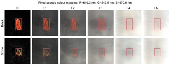
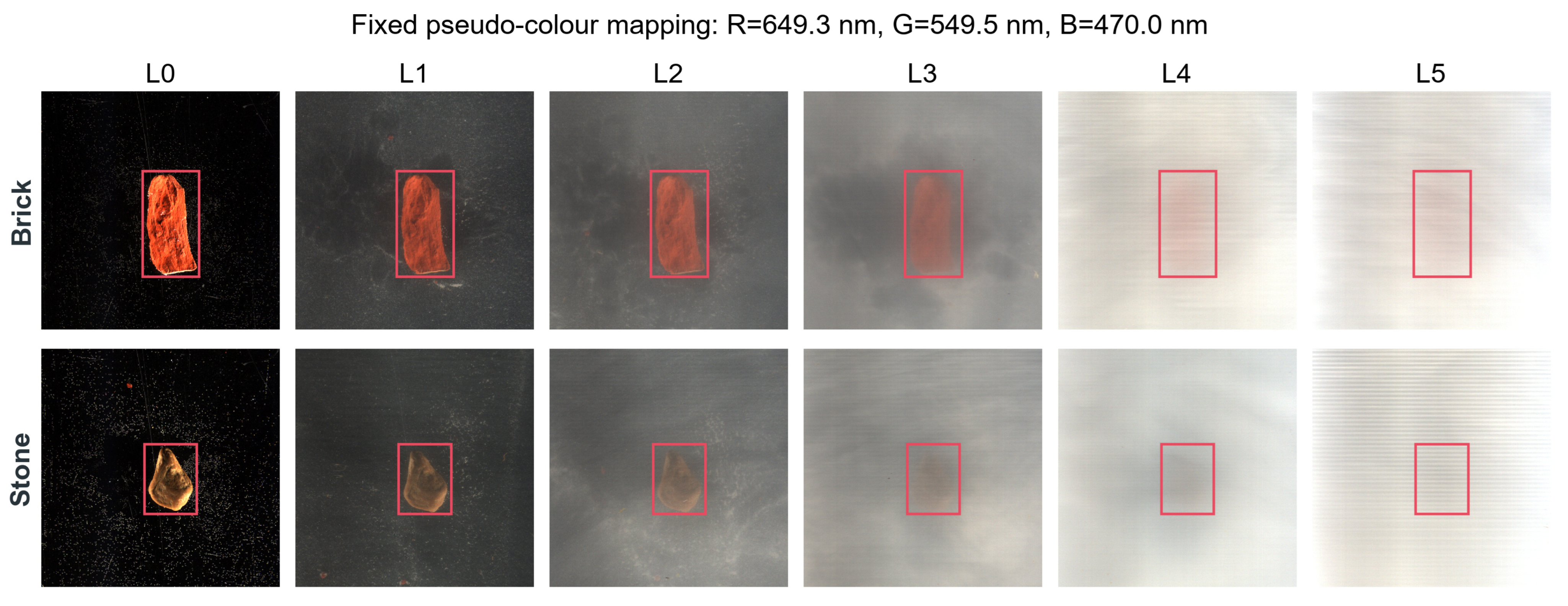
L0 served as the labeled source, and L1–L5 formed the ordered unlabeled target domains. For each sequence, the target prior was obtained by averaging the 1296 spectra within a $36\times 36$-pixel patch inside the L0 target region. The resulting 181-dimensional spectrum remained fixed throughout adaptation. Figure 5 shows representative inputs across the turbidity gradient.

Figure 5. Representative L0–L5 inputs using fixed R/G/B bands at 649.3/549.5/470.0 nm and common display limits. Red boxes locate targets for visualization only.

The source model was trained with Adam using a learning rate of ${10}^{-4}$, weight decay of ${10}^{-4}$, and batch size 1024. The linear decoder used 0.1 times the current learning rate. Source training ran for 50 epochs, followed by 30 adaptation epochs at each target level, divided into three rounds of ten epochs. Adaptation used a learning rate of $5\times {10}^{-6}$; each epoch used at most 150 mini-batches, further limited by the selected-anchor loader length. Teacher and prototype momenta were 0.995 and 0.90, respectively.

The spatial-field estimator used a $1\to 8\to 16\to 8\to 8\to 1$ channel architecture on $256\times 256$ inputs. It was trained for 120 steps at a learning rate of ${10}^{-3}$, with TV weight 0.05, target-smoothing width 5 pixels, and row-residual smoothing width 1.5 pixels. The correction strength was $\gamma =0.70$, with coefficients clipped to [0.70,1.40]. The background-context network used 12,000 patches per epoch sampled from the lowest 70% of initial responses. It was trained for eight epochs with batch size 128 and learning rate $5\times {10}^{-4}$. PCA used three components estimated from up to 50,000 sampled spectra. The per-class pseudo-anchor fractions for L1–L5 were 0.010, 0.0125, 0.015, 0.020, and 0.025, respectively.

RG-OBS searched seed percentiles 99.8, 99.7, 99.5, 99.3, and 99.0, retaining up to five seed components at each threshold. Allowable growth masks used percentiles 92, 90, 88, 85, 82, 80, 75, and 70; core dilation used a seven-pixel radius. The brick, stone, and generic presets used distance-decay scales/support radii of 25/32, 40/45, and 30/35 pixels, respectively. Their soft/hard area caps were 3.5/5.0, 4.0/6.0, and 4.0/6.0 times $A_0$; the small-stone branch used 3.0/4.5. The candidate-area utility used 0.35$A_0$ as a reference bound, not a hard rejection threshold; areas below 0.25$A_0$ triggered the final input-preserving fallback. Far-field retention was 0.08. Conditional SGR at L4–L5 used 24 iterations, a 35-pixel candidate radius, and foreground threshold 0.52. These presets were fixed across levels and seeds; no target-domain evaluation labels were used to select them.

Learning-based methods were evaluated with seeds 36–40. Within each seed, results were averaged equally over 13 targets and five target-domain levels, yielding 65 scenes. We report the mean and sample standard deviation across the five seed-wise averages. Level-wise results were first averaged over targets and then summarized across seeds. The five classical detectors produced deterministic responses; their ranking scores were computed once, whereas variation in source metrics reflected the five shared L0 calibration subsets.

4.2. Evaluation Metrics

Ranking was evaluated by the area under the receiver-operating-characteristic curve (AUROC) and average precision (AP). AP, also reported as AUPR in the ablations, was computed without trapezoidal interpolation:

$$\mathrm{AP}=\mathrm{AUPR}={\displaystyle \sum _{k=1}^K}(R_k-R_{k-1})P_k,R_0=0.$$

(62)

Here, $P_k$ and $R_k$ denote precision and recall at successive distinct score thresholds. With TP, FP, TN, and FN denoting true/false positives/negatives, thresholded metrics were $\mathrm{Precision}=\mathrm{TP}/(\mathrm{TP}+\mathrm{FP})$, $\mathrm{Recall}=\mathrm{TP}/(\mathrm{TP}+\mathrm{FN})$, $F_1=2\mathrm{TP}/(2\mathrm{TP}+\mathrm{FP}+\mathrm{FN})$, and $\mathrm{FPR}=\mathrm{FP}/(\mathrm{FP}+\mathrm{TN})$.

Boundary F1 combines boundary precision and recall with a two-pixel tolerance. It measures agreement with the transferred reference contours, rather than independently annotated target-domain boundaries. Mean background response is the average scene-normalized score outside the target mask and quantifies residual background activation.

To compare source-threshold transfer consistently, all methods used the same L0 calibration pixels for each target and seed: 180 target pixels and 180 background pixels. Each model’s threshold maximized F1 on these 360 source pixels, with ties resolved by choosing the highest threshold. Native saved responses were used without scene-wise min–max normalization. The shared protocol therefore standardized calibration pixels and the selection rule, rather than imposing one numerical threshold on all methods.

For Full and the other sequence systems, the source-model threshold was frozen along L1–L5; HUTDNet-based likewise retained its L0 model and threshold. DANN, TSDA, and SVHAE fitted a separate model for each target level. Each fitted model was evaluated on the same L0 calibration indices to obtain its own threshold, which was applied to the corresponding target level. Target-domain evaluation labels were not used to select these operating points. The calibration subset belonged to the source training domain and was not a held-out validation set.

The ablation and historical mask-perturbation analyses used full-L0 threshold selection after scene-wise normalization. The additional boundary checks used native scores and common L0 calibration subsets. Their operating-point F1 values are reported separately.

Adaptive F1 uses an unlabeled selector based on response strength, target support, L0 area consistency, and component plausibility. F1@0.4/0.6 applies fixed normalized-score thresholds. Oracle Best F1 is the offline maximum over target thresholds; Pd@FAR = 0.001 is the highest evaluated detection rate below the false-alarm limit. These last two are evaluation diagnostics, not deployment thresholds.

Paired analyses used 13 physical targets after averaging seeds and levels within each target. Exact two-sided signed-rank permutation tests enumerated all 8192 sign assignments, using average ranks for tied absolute differences. Holm correction covered ten comparators for AP and Source F1 (20 tests); pointwise 95% intervals used 20,000 paired target-bootstrap resamples. Full’s AP advantage over SVHAE was 0.0710 (95% CI 0.0302–0.1054; adjusted p = 0.0161), providing statistical support for the observed AP advantage under this protocol.

4.3. Comparative Experiments

The comparison retained the five conventional detectors SAM, CEM, ACE, MF, and OSP [4,5,6,7,8]; the nonlinear-unmixing baseline NUN-UTD [16]; and four additional learning methods. HUTDNet combines hyperspectral unmixing with target detection [17]. SVHAE uses a spectral-variability-aware hybrid autoencoder to model underwater spectral variation [32]. DANN learns domain-adapted features through adversarial training [33], while TSDA combines self-distillation and test-time adaptation in a two-stage framework [34]. Together with Full, these eleven systems cover conventional spectral detection, learned unmixing, and domain adaptation.

All methods were evaluated on the same cubes, spatial crops, transferred masks, and common L0 calibration subsets. SVHAE and HUTDNet-based, marked with an asterisk, were independently implemented for the present task. HUTDNet-based was trained using L0 supervision and applied directly to L1–L5 without target-domain adaptation. DANN and TSDA adapted independently from L0 to each target level, whereas Full inherited states along the ordered sequence. Architectures, supervision amounts, and training budgets were method-specific. These results compare the declared implementations rather than reproduce every method’s complete published protocol; the matched controls in Section 4.5 more directly examine adaptation routing and module contributions.

DANN used a spectral-network adaptation with batch size 256 for 20 epochs and 150 updates per epoch. TSDA was adapted from the authors’ code to binary detection with $7\times 7$ patches and 180 labeled L0 pixels per class. Its first stage used 50 epochs and batch size 32. Test-time adaptation performed one update in 223 tasks, two in 81, and none in 21; all 325 outcomes were retained.

SVHAE was fitted independently at each target level for 100 epochs with batch size 4096, using the L0 target prior, VCA initialization, and equal numbers of original and synthetic spectra. The independent implementation used convex-mixing coefficients sampled from $U(0.2,0.6)$ and equally weighted KL, MSE, and spectral-angle reconstruction terms. HUTDNet-based was trained on L0 for 100 epochs with batch size 2048 and $9\times 9$ patches. It used BF16 training and FP32 evaluation before direct application to L1–L5. Initial learning rates were 0.01 for DANN, 0.1 for TSDA, and ${10}^{-4}$ for both SVHAE and HUTDNet-based. DANN used 3000 joint updates/model; SVHAE and HUTDNet-based each used 31,300 updates per fitted model. Historical NUN-UTD budgets and Full optimizer totals were not fully recoverable. These are task-specific implementations with method-specific training budgets, rather than exact reproductions of the original training protocols.

Across the 65 target-domain scenes (Table 2), Full achieved AP = $0.9282\pm 0.0009$ and AUROC = $0.9773\pm 0.0009$. Its AP exceeded the strongest external comparator, SVHAE, by 7.10 percentage points. MF was the strongest external comparator by aggregate AUROC (0.9601). These comparisons support an aggregate advantage under the evaluated conditions, rather than superiority for every target or level.

Table 2. Overall ranking and operating-point results with shared L0 calibration on L1–L5. AP, average precision; AUROC, area under the receiver operating characteristic curve; FPR, false-positive rate.

Method	AUROC ↑	AP ↑	Source F1 ↑	Source Recall ↑	Source FPR ↓	Source Boundary F1 ↑
SAM	0.8713	0.7242	0.2483 ± 0.0350	0.5199 ± 0.0416	0.3273 ± 0.0777	0.0625 ± 0.0049
CEM	0.9011	0.6925	0.4099 ± 0.0127	0.4507 ± 0.0217	0.0907 ± 0.0052	0.0739 ± 0.0058
ACE	0.9099	0.6811	0.3122 ± 0.0166	0.9435 ± 0.0085	0.4219 ± 0.0291	0.0140 ± 0.0012
MF	0.9601	0.8047	0.3767 ± 0.0375	0.4547 ± 0.0202	0.1309 ± 0.0367	0.0685 ± 0.0049
OSP	0.5444	0.1155	0.1494 ± 0.0002	0.9953 ± 0.0034	0.9936 ± 0.0051	0.0092 ± 0.0017
NUN-UTD	0.7057 ± 0.0522	0.4619 ± 0.0507	0.1566 ± 0.0077	0.6596 ± 0.1664	0.5903 ± 0.1731	0.0143 ± 0.0036
SVHAE *	0.9521 ± 0.0161	0.8571 ± 0.0224	0.2346 ± 0.0186	0.4266 ± 0.0274	0.2192 ± 0.0295	0.0468 ± 0.0112
HUTDNet-based *	0.7563 ± 0.0288	0.5827 ± 0.0334	0.2865 ± 0.0309	0.6135 ± 0.0302	0.3940 ± 0.0622	0.0665 ± 0.0091
DANN	0.6937 ± 0.0376	0.5055 ± 0.0378	0.2000 ± 0.0123	0.8402 ± 0.0522	0.7390 ± 0.0443	0.0226 ± 0.0108
TSDA	0.5562 ± 0.0190	0.2623 ± 0.0173	0.1994 ± 0.0133	0.9829 ± 0.0179	0.8954 ± 0.0178	0.0298 ± 0.0071
Ours (Full)	0.9773 ± 0.0009	0.9282 ± 0.0009	0.7750 ± 0.0236	0.7942 ± 0.0449	0.0286 ± 0.0113	0.2020 ± 0.0236

Mean ± sample SD over five seed-wise macro averages of 65 L1–L5 scenes. The 180 L0 target and 180 L0 background pixels per target/seed are used only to calibrate thresholds. Source F1, recall, FPR, and Boundary F1 are evaluated on the L1–L5 target-domain images using native scores. Classical ranking scores are deterministic; their source SD reflects calibration sampling. * Independent task-adapted implementations, as defined in Section 4.3. ↑ indicates that higher values are better; ↓ indicates that lower values are better. Bold values indicate the best result in each column.

Under shared L0 calibration, Full achieved Source F1 = 0.7750 ± 0.0236, precision = 0.8339 ± 0.0277, recall = 0.7942, FPR = 0.0286, and Boundary F1 = 0.2020. It had the highest mean Source F1 and Boundary F1 and the lowest mean FPR among the eleven methods. SVHAE obtained Source F1 = 0.2346 ± 0.0186 and FPR = 0.2192. TSDA combined recall = 0.9829 with FPR = 0.8954, illustrating that high recall alone did not establish accurate foreground separation. These common-calibration results complement the ranking measures; Table 3 further separates offline discrimination potential from source-threshold transfer.

Table 3. Offline best-F1 and low-false-alarm detection diagnostics. Pd@FAR denotes detection probability at a specified false-alarm rate.

Method	Oracle Best F1 ↑	Pd@FAR = 0.001 ↑
SAM	0.7218	0.4213
CEM	0.6914	0.2798
ACE	0.6693	0.3162
MF	0.7703	0.3567
OSP	0.1860	0.0052
NUN-UTD	0.4864 ± 0.0376	0.2335 ± 0.0275
SVHAE *	0.8257 ± 0.0181	0.5390 ± 0.0241
HUTDNet-based *	0.6136 ± 0.0285	0.2381 ± 0.0363
DANN	0.5284 ± 0.0331	0.2447 ± 0.0171
TSDA	0.3564 ± 0.0131	0.0848 ± 0.0169
Ours (Full)	0.8906 ± 0.0008	0.6225 ± 0.0014

Both columns are offline diagnostics using target labels; neither defines a deployment threshold. Aggregation follows Table 2. ↑ indicates that higher values are better. Bold values indicate the best result in each column. An asterisk marks an independent task-adapted implementation, as described in Section 4.3.

Full also led the aggregate offline diagnostics in Table 3, with Oracle Best F1 = 0.8906 and Pd@FAR = 0.001 of 0.6225. The difference between offline-best and source-calibrated F1 distinguishes ranking quality from operating-point transfer.

4.4. Detection Performance and Spatial Responses Across Turbidity Levels

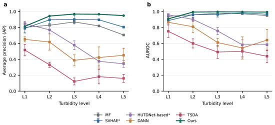
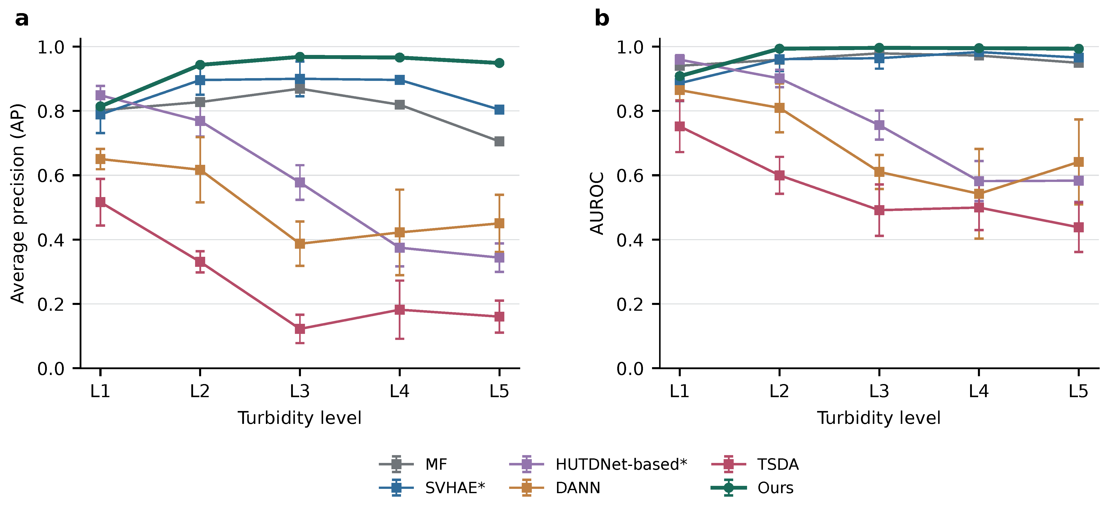
Full led all eleven methods in mean AP, AUROC, Source F1, and Source Boundary F1 at L4–L5 (Figure 6). Its AP reached 0.9661 and 0.9491, exceeding SVHAE by 6.96 and 14.49 percentage points, respectively. Full led mean AP and AUROC from L2 to L5, whereas HUTDNet-based performed better at L1 (AP 0.8486 versus 0.8141).

Figure 6. (a) AP and (b) AUROC across L1–L5. Each stochastic-method point is the mean of five seed-wise averages over 13 targets; error bars are sample standard deviations. MF is deterministic. Six representative methods are shown for readability; all eleven methods are included in Table 2. * Implementation definitions follow Table 2.

4.4.1. Qualitative Response Analysis

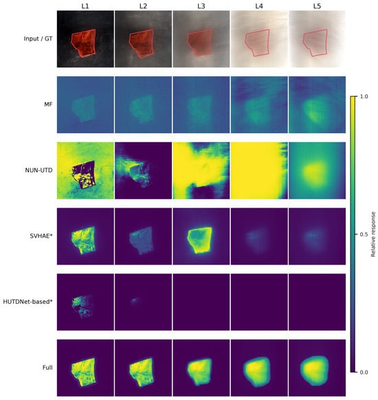
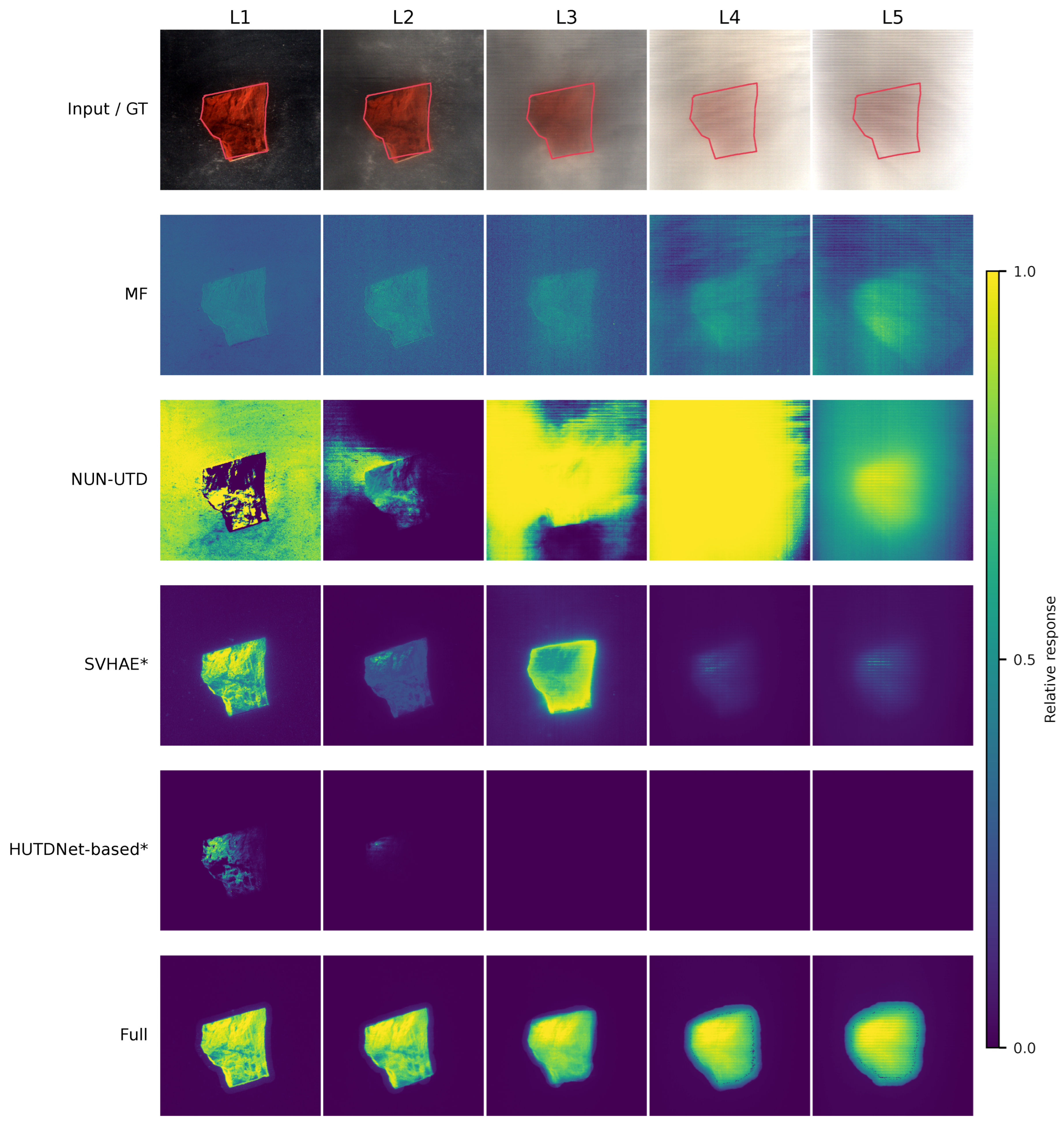
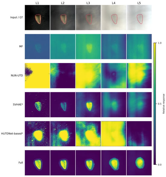
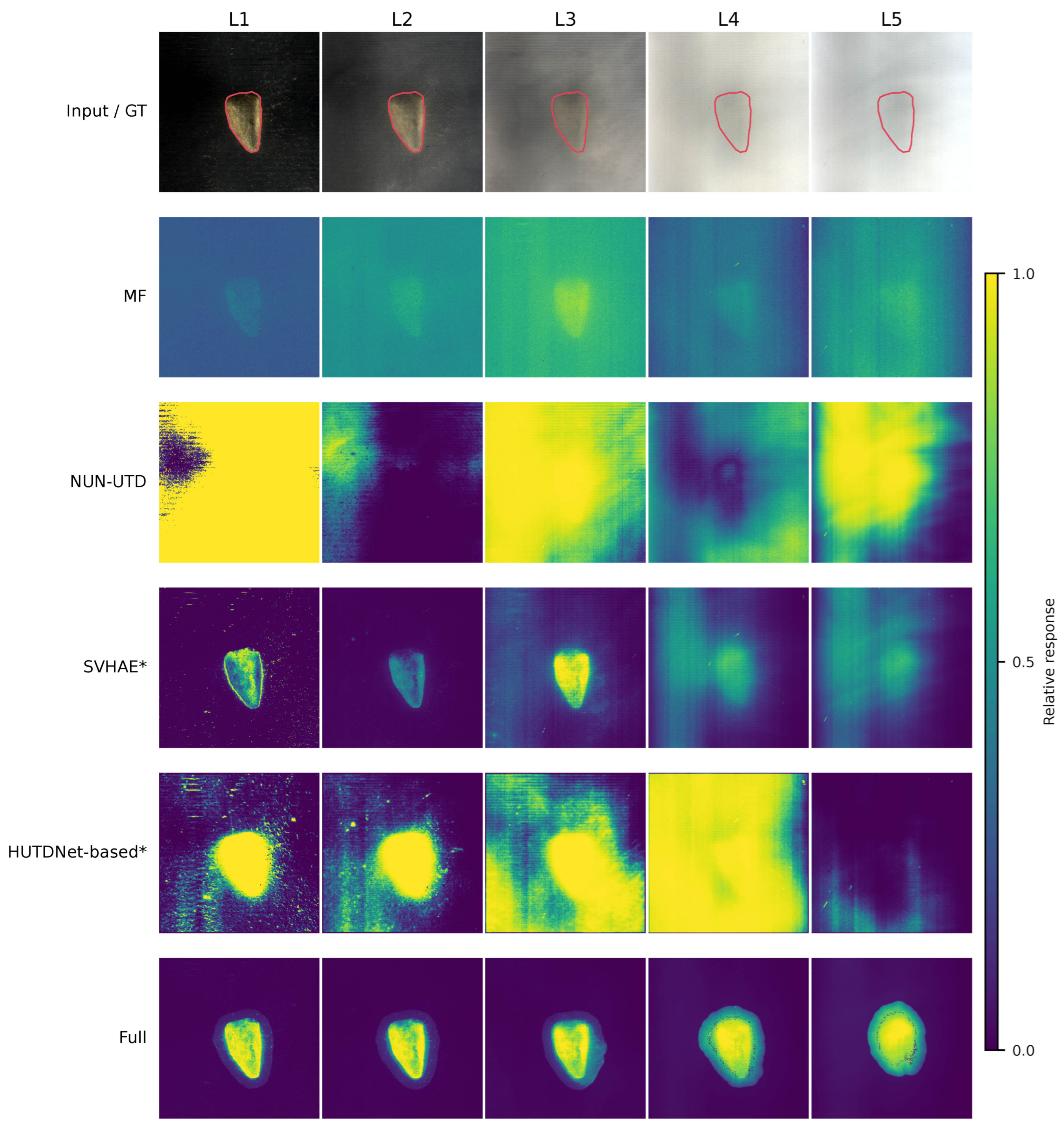
Figure 7 and Figure 8 compare five detectors on brick1 and stone4 (seed 36). Full retained a localized brick1 response as turbidity increased, whereas MF showed weaker contrast and NUN-UTD varied more across levels. Full fields of view are preserved; scene-wise response normalization shows relative spatial contrast, not probabilities calibrated across methods.

Figure 7. Brick1 L1–L5 input/GT and responses of MF, NUN-UTD, SVHAE*, HUTDNet-based*, and Full (seed 36). RGB bands are 649.33/549.45/470.00 nm, with pooled display limits shared with Figure 8. Red contours are evaluation references; continuous responses use scene-wise min–max display only. GT (ground-truth reference) denotes the evaluation mask transferred from L0, without independent target-domain annotation. An asterisk marks an independent task-adapted implementation, as described in Section 4.3.

Figure 8. Stone4 L1–L5 input/GT and responses of MF, NUN-UTD, SVHAE*, HUTDNet-based*, and Full (seed 36). The method selection, RGB bands, pooled input-display limits, and scene-wise min–max response display match Figure 7. GT (ground-truth reference) denotes the evaluation mask transferred from L0, without independent target-domain annotation. An asterisk marks an independent task-adapted implementation, as described in Section 4.3.

Full similarly retained the main stone4 response despite declining visibility, while comparator maps showed background expansion, striping, or weakened contrast. Visual darkness alone does not establish poor ranking: HUTDNet-based obtained AP = 0.9762 on brick1/L2 despite Source F1 = 0, illustrating imperfect source-threshold transfer.

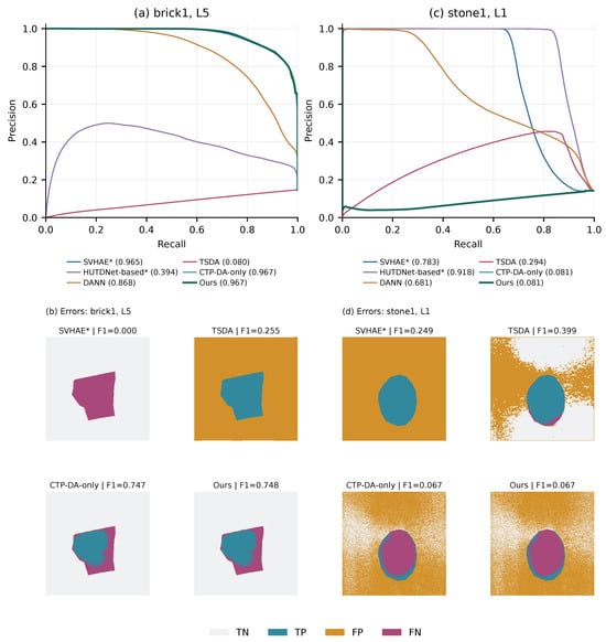
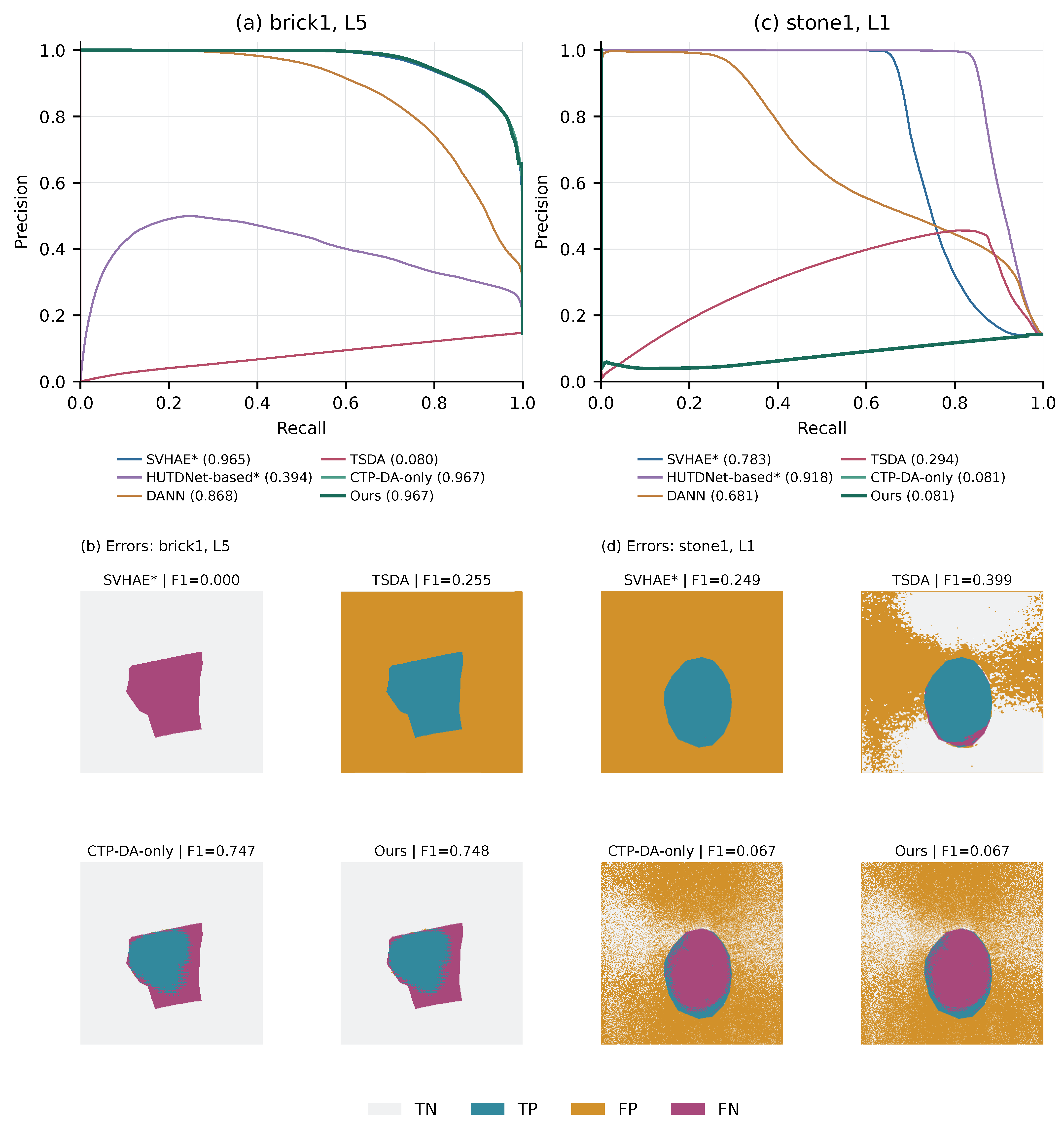
Figure 9 separates ranking from source-threshold errors. On brick1/L5, SVHAE, CTP-DA-only, and Full had similar AP (0.965–0.967), but Full obtained Source F1 = 0.7483 while SVHAE missed the target at its source threshold. On stone1/L1, CTP-DA-only and Full both had AP $\approx 0.081$ and Source F1 $\approx 0.0669$, showing the dependence of calibration on upstream ranking. Section 4.5 isolates RG-OBS using matched inputs.

Figure 9. Precision–recall (PR) curves and spatial errors for brick1/L5 and stone1/L1 (seed 36). Errors use native scores and common 180+180 L0 calibration. TN/TP/FP/FN denote true negatives, true positives, false positives, and false negatives. PR curves are case-specific. CTP-DA-only and Full are separately evaluated versions, not a matched-input RG-OBS estimate. An asterisk marks an independent task-adapted implementation, as described in Section 4.3.

4.4.2. Sensitivity to Transferred-Mask Perturbations

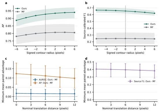
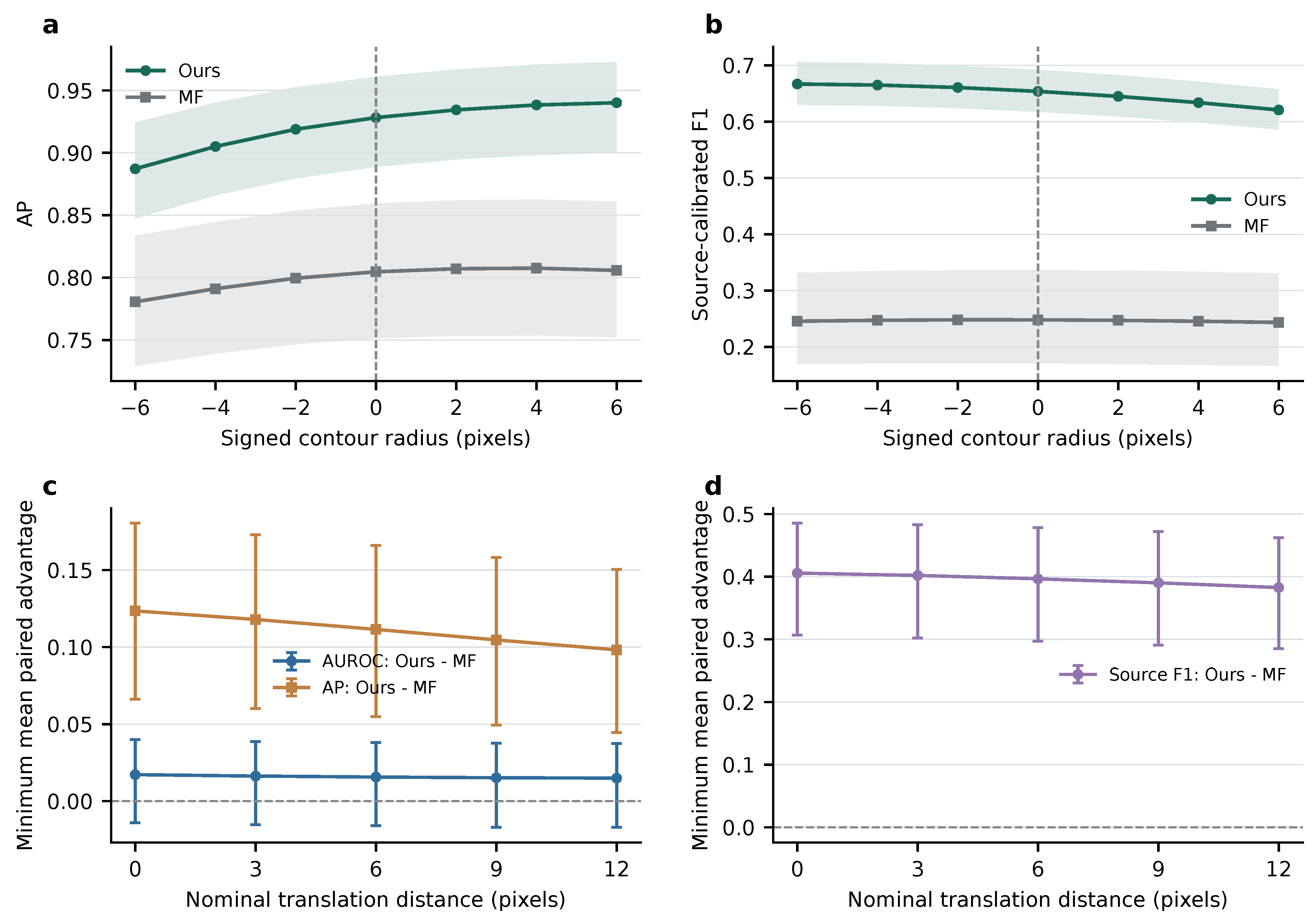
With detector response maps held fixed, the historical full-L0 normalized-score analysis yielded AP values of 0.8871–0.9401 under contour perturbations (Figure 10). At the largest nominal translation of 12 pixels, the least favorable directional mean advantages over MF were 0.0981 for AP and 0.3825 for Source F1. The corresponding pointwise 95% target-bootstrap intervals were above zero for both metrics, whereas the AUROC interval crossed zero.

Figure 10. Mask perturbations against MF: contour erosion/dilation (a,b) and least favorable mean paired differences across eight translation directions (c,d). Shading/bars are 95% target-sequence bootstrap intervals. Only evaluation masks changed; original full-L0 calibration applies.

Additional native-score checks used common 180+180 L0 calibration. For disk-morphology contour offsets of −6, −4, −2, 0, +2, +4, and +6 pixels, Full Boundary F1 was 0.1370, 0.1631, 0.1895, 0.2020, 0.1964, 0.1776, and 0.1515, respectively, at two-pixel tolerance. With the unperturbed reference mask, square-neighborhood tolerances of 2, 5, and 10 pixels gave Full Boundary F1 of 0.2020, 0.3470, and 0.5010, respectively. Paired pointwise 95% intervals for Full minus each comparator (SVHAE and MF) remained above zero across the tested contour offsets and matching tolerances; absolute boundary scores remained reference-dependent.

4.5. Ablation Study

4.5.1. Ablation Protocol

We first compared five configurations to separate adaptation from output calibration (Table 4). Base AE applied the source-trained autoencoder directly to L1–L5. Adding CTP-DA introduced progressive adaptation and its conditional output-only core–halo calibration; adding RG-OBS alone calibrated the unadapted responses. Full combined the two modules. Direct-DA independently adapted the L0 model to each target level for 30 epochs, providing a same-backbone route comparison. All configurations used the same 13 target sequences, source priors, and seeds 36–40.

Table 4. Overall contributions of CTP-DA, RG-OBS, and adaptation routing.

Configuration	AUROC ↑	AUPR ↑	Adaptive F1 ↑	Mean BG ↓	F1@0.4 ↑	F1@0.6 ↑
Base AE	0.6318 ± 0.0489	0.4645 ± 0.0467	0.6039 ± 0.0467	0.4392 ± 0.0191	0.3673 ± 0.0251	0.3986 ± 0.0298
Base AE + CTP-DA	0.9691 ± 0.0002	0.9103 ± 0.0004	0.8966 ± 0.0004	0.1927 ± 0.0018	0.6761 ± 0.0037	0.7882 ± 0.0030
Base AE + RG-OBS	0.6433 ± 0.0473	0.4761 ± 0.0497	0.4589 ± 0.0544	0.1306 ± 0.0128	0.4230 ± 0.0428	0.4199 ± 0.0421
Direct-DA	0.9638 ± 0.0009	0.8712 ± 0.0041	0.8638 ± 0.0094	0.2445 ± 0.0014	0.5979 ± 0.0015	0.7013 ± 0.0063
Full	0.9773 ± 0.0009	0.9282 ± 0.0009	0.8932 ± 0.0072	0.0528 ± 0.0040	0.8066 ± 0.0023	0.8354 ± 0.0021

Five-seed macro means ± sample SD. Adaptive F1 uses an unlabeled selector; F1@0.4/0.6 uses normalized-score thresholds. ↑ indicates that higher values are better; ↓ indicates that lower values are better. Bold values indicate the best mean in each column.

Internal CTP-DA interventions reran the full adaptation sequence and used a matched rerun default. In contrast, RG-OBS interventions and parameter scans reused identical frozen upstream responses, so their differences arose after response construction. Each comparison retained its corresponding full-L0 source threshold across L1–L5. Table 4 reports the original module-level runs, while Table 5 separates the matched internal comparisons.

Table 5. Selected internal mechanisms and a matched-input calibration control.

(A) CTP-DA with RG-OBS Disabled
Configuration	AUPR ↑	Source F1 ↑	Source Boundary F1 ↑	Source FPR ↓	Mean BG ↓
Default CTP-DA	0.9103 ± 0.0004	0.6517 ± 0.0198	0.1135 ± 0.0097	0.00665 ± 0.00195	0.1927 ± 0.0018
No spatial memory	0.8672 ± 0.0048	0.6011 ± 0.0165	0.0855 ± 0.0049	0.01082 ± 0.00211	0.2297 ± 0.0019
Equal expert weights	0.8081 ± 0.0048	0.4793 ± 0.0167	0.1418 ± 0.0037	0.00910 ± 0.00180	0.2350 ± 0.0011
Frozen L0 prototype	0.9115 ± 0.0005	0.6514 ± 0.0197	0.1132 ± 0.0095	0.00627 ± 0.00177	0.1923 ± 0.0018
No spectral contrast	0.7644 ± 0.0019	0.5372 ± 0.0180	0.0992 ± 0.0063	0.06757 ± 0.00793	0.2526 ± 0.0027
No background context	0.9098 ± 0.0004	0.6481 ± 0.0205	0.1087 ± 0.0102	0.00673 ± 0.00194	0.1917 ± 0.0020
(B) RG-OBS with frozen upstream predictions
Configuration	AUPR ↑	Source F1 ↑	Source Boundary F1 ↑	Source FPR ↓	Mean BG ↓
Default RG-OBS	0.9282 ± 0.0009	0.6537 ± 0.0204	0.1173 ± 0.0098	0.00429 ± 0.00172	0.0528 ± 0.0040
Identity of RG input	0.9103 ± 0.0004	0.6517 ± 0.0198	0.1134 ± 0.0097	0.00665 ± 0.00195	0.1927 ± 0.0018
No risk gate	0.9296 ± 0.0008	0.6537 ± 0.0204	0.1174 ± 0.0097	0.00429 ± 0.00172	0.0486 ± 0.0041
No additional boundary protection	0.9282 ± 0.0009	0.6537 ± 0.0204	0.1173 ± 0.0098	0.00429 ± 0.00172	0.0528 ± 0.0040
No SGR	0.9302 ± 0.0002	0.6550 ± 0.0199	0.1186 ± 0.0101	0.00431 ± 0.00176	0.0524 ± 0.0040

Five-seed macro means ± sample SD under full-L0, scene-normalized calibration. A reruns CTP-DA with RG-OBS disabled; B uses frozen upstream predictions. Identity retains the exact RG input. Other rows disable the named operation; no-risk-gate retains candidate checks. SGR is L4–L5 seeded graph refinement. ↑ indicates that higher values are better; ↓ indicates that lower values are better. Bold rows identify the default configurations and do not indicate column-wise optima.

4.5.2. Overall Module Contributions and Adaptation Routing

CTP-DA provided the principal module-level improvement (Table 4), raising AUPR from 0.4645 to 0.9103 and Adaptive F1 from 0.6039 to 0.8966. RG-OBS applied directly to Base AE reached only AUPR = 0.4761 and Adaptive F1 = 0.4589, so output calibration alone did not recover the adaptation benefit.

Full achieved the highest AUROC and AUPR among the five configurations (0.9773 and 0.9282). After RG-OBS, mean background response fell from 0.1927 to 0.0528; F1@0.4 and F1@0.6 rose to 0.8066 and 0.8354. Adaptive F1 decreased slightly from 0.8966 to 0.8932, indicating threshold-dependent calibration benefits.

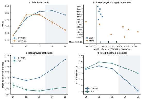
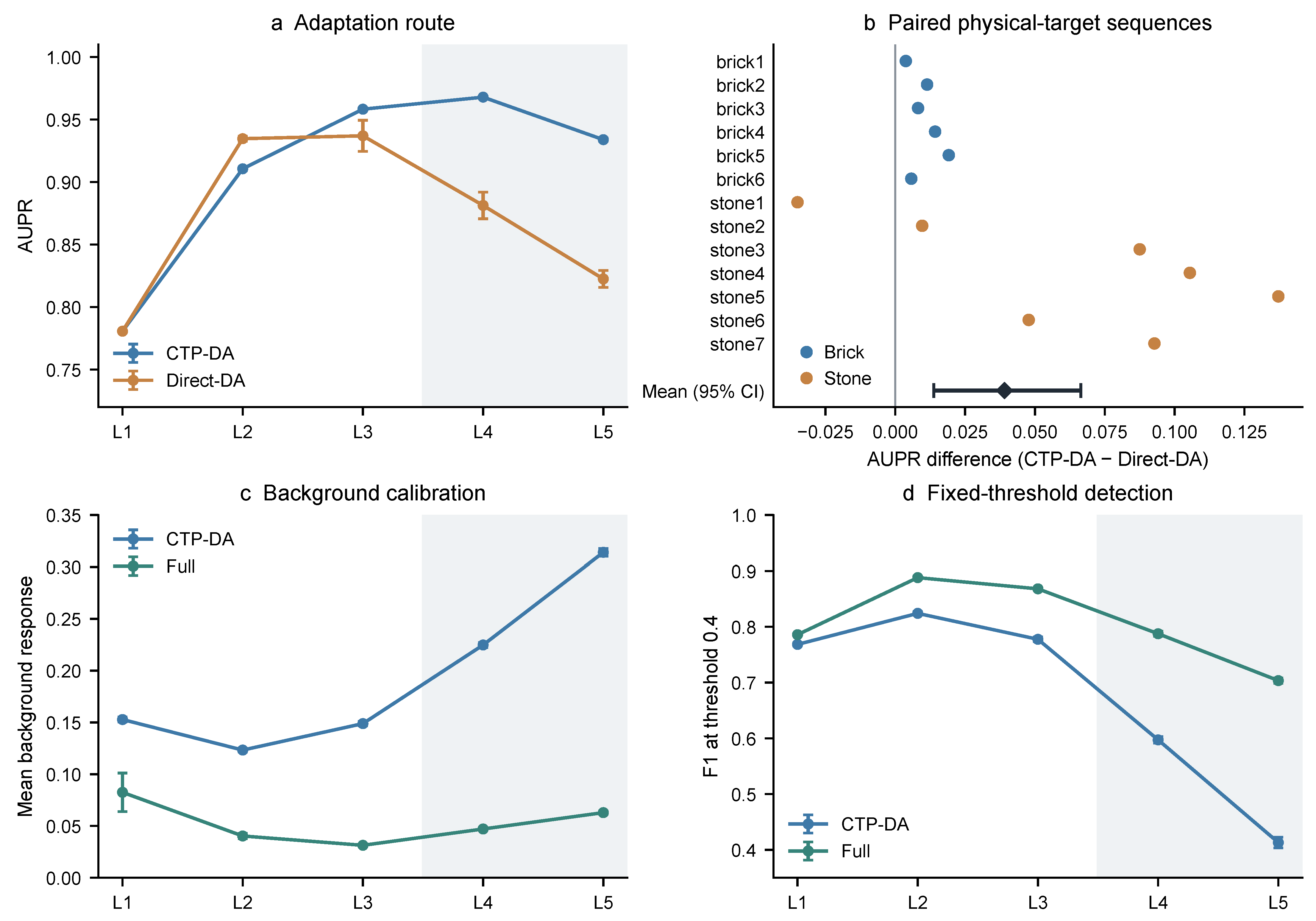
At L5, CTP-DA achieved AUPR = 0.9339 versus 0.8225 for Direct-DA (Figure 11a,b), although the routes differed in cumulative adaptation budget. RG-OBS then reduced background response from 0.3140 to 0.0629 and increased F1@0.4 from 0.4131 to 0.7035 (Figure 11c,d), supporting complementary adaptation and calibration roles.

Figure 11. CTP-DA versus Direct-DA across levels (a) and paired target-sequence AUPR differences (b); CTP-DA versus Full background response (c) and F1@0.4 (d). Bars in (a,c,d) are five-seed sample SD; (b) shows a 95% interval from 20,000 target-sequence bootstrap resamples. Gray shading marks L4–L5.

4.5.3. Selected Internal Mechanisms of CTP-DA

To examine the mechanisms within CTP-DA, we removed spatial memory, replaced reliability-weighted fusion with equal expert weights, froze the L0 prototype, or removed spectral contrast or background context (Table 5A). Equal weighting retained all evidence branches but changed their final combination; branch-removal variants renormalized the remaining experts. This design separates the contribution of evidence construction from the use of historical responses and reliability-dependent fusion.

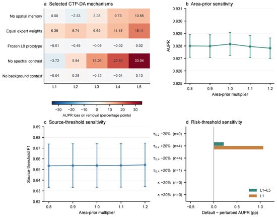
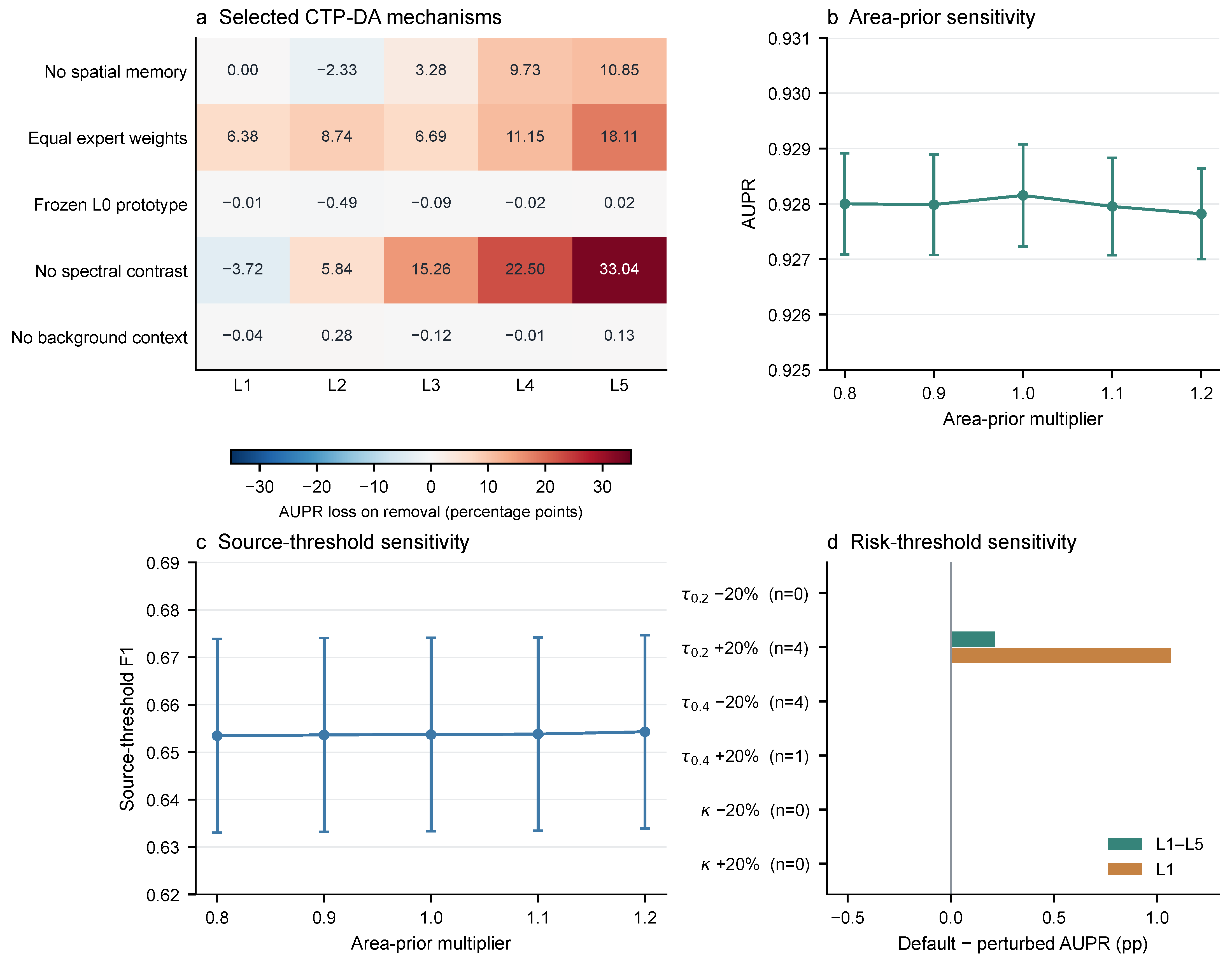
Reliability-weighted fusion, spatial memory, and spectral contrast provided the clearest aggregate ranking contributions (Table 5A). Equal expert weighting reduced AUPR by approximately 10.2 percentage points; removing spatial memory and spectral contrast reduced it by 4.31 and 14.59 points, respectively. The latter two removals reduced L4–L5 AUPR by 10.29 and 27.77 percentage points, respectively (Figure 12a). These comparisons support reliability-aware evidence fusion, historical spatial responses, and spectral contrast within the tested progressive adaptation procedure.

Figure 12. CTP-DA intervention losses (a), area-prior sensitivity (b,c), and risk-threshold sensitivity (d). Negative default-minus-variant values favor the variant. Error bars show five-seed sample SD; n counts changed gate decisions. Panel (a) reruns adaptation; (b–d) freeze upstream inputs and source thresholds.

The remaining intervention effects depended on the metric and target sequence. Equal weighting increased Source Boundary F1 from 0.1135 to 0.1418 but reduced Source F1 from 0.6517 to 0.4793, alongside the aggregate AUPR loss. Per-target averages over seeds and levels showed lower AUPR for all seven stone sequences after spectral-contrast removal, alongside small increases for the six brick sequences. Removing background context reduced L4–L5 Source F1 from 0.7062 to 0.6936 and Source Boundary F1 from 0.0946 to 0.0846. This supports its auxiliary contribution to thresholded spatial detection at high turbidity. Freezing the L0 prototype yielded AUPR of 0.9115, compared with 0.9103 for the default. The tested protocol therefore did not establish an independent aggregate ranking gain from prototype updating.

For brick1 and stone1 with seeds 36–38, 18 CTP-DA sequences before RG-OBS gave mean AP of 0.862157, 0.862322, and 0.862558 at replay weights 6.4, 8, and 9.6. Mean AP varied only slightly over this tested range; the maximum absolute scene/seed Source F1 difference from weight 8 was 0.13394, indicating less uniform operating-point stability.

4.5.4. Internal Analysis of RG-OBS

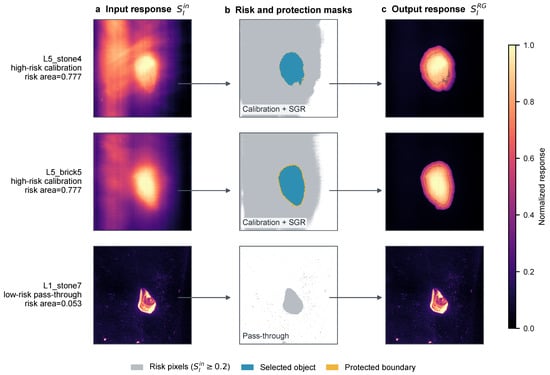
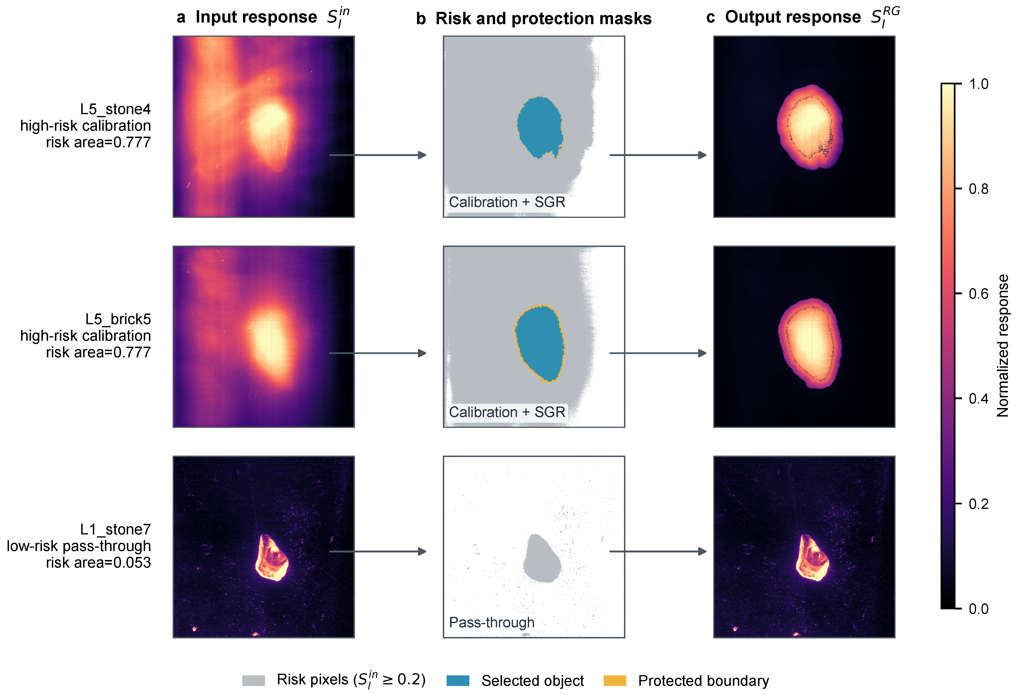
The matched-input identity control leaves the RG-OBS input $S_l^{\mathrm{in}}$ unchanged, including any accepted core–halo calibration (Table 5B). Relative to this control, complete RG-OBS increased AUPR from 0.9103 to 0.9282 and reduced mean background response from 0.1927 to 0.0528. Source FPR decreased from 0.00665 to 0.00429, while Source F1 and Source Boundary F1 increased from 0.6517 to 0.6537 and from 0.1134 to 0.1173, respectively. With upstream prediction, normalization, and source thresholds shared, this comparison isolates the overall contribution of RG-OBS. Figure 13 illustrates its selective suppression and low-risk pass-through behavior across representative scenes.

Figure 13. RG-OBS inputs, risk/candidate/protection states, and calibrated outputs (seed 36). L5_stone4/L5_brick5 show suppression; L1_stone7 shows pass-through. Shared response limits are [0,1]; gray/blue/yellow indicate risk pixels/selected objects/protected boundaries.

The gate controls conditional object search, while SGR refines supported candidates at L4–L5. Their interventions produced small, metric-dependent changes (Table 5), rather than uniform independent accuracy gains. Background context assisted in high-turbidity spatial detection, as shown in Section 4.5.3. Single-operation interventions do not establish equivalence after joint removal.

We also examined calibration sensitivity. Area-prior multipliers of 0.8–1.2 kept AUPR within 0.9278–0.9282 and Source F1 within 0.6535–0.6543 (Figure 12b,c). One-at-a-time ±20% risk-threshold perturbations changed zero to four of 325 gate decisions; the largest reported L1 AUPR loss was 1.07 points (Figure 12d). This indicates aggregate stability within the tested range, with local routing sensitivity.

4.6. Evaluation on Wooden Targets and Altered Illumination

We evaluated Full on the wooden targets and illumination conditions defined in Section 2.1 using the same configuration as the primary experiments. Each sequence started from its own labeled L0, target prior, and source threshold, followed by adaptation through L1–L5. Results were summarized over seeds 36–40 and analyzed separately from the 13-target benchmark. The wooden-target macro average weighted the three specimens equally.

4.6.1. Detection of Wooden Targets

Full maintained high ranking performance on all three wooden targets (Table 6), with macro-average AP = 0.9461, AUROC = 0.9931, and Source F1 = 0.7950. These results extend the tested materials under the same target-specific training and adaptation procedure.

Table 6. Wooden-target results over L1–L5 and at L5.

Target	Overall AP	Overall AUROC	Overall Source F1	L5 AP	L5 Source F1
branch1	0.9338 ± 0.0128	0.9892 ± 0.0024	0.7778 ± 0.0429	0.8752 ± 0.0563	0.7121 ± 0.0878
branch2	0.9474 ± 0.0007	0.9946 ± 0.0001	0.7539 ± 0.1584	0.9501 ± 0.0021	0.7484 ± 0.0739
branch3	0.9572 ± 0.0006	0.9956 ± 0.0001	0.8533 ± 0.0488	0.9657 ± 0.0021	0.8127 ± 0.0792
Macro average	0.9461 ± 0.0043	0.9931 ± 0.0008	0.7950 ± 0.0473	0.9303 ± 0.0184	0.7577 ± 0.0343

Five-seed means ± sample SD; overall averages L1–L5, and the macro row weights specimens equally. Source F1 uses each sequence’s common-subset L0 threshold. Full only.

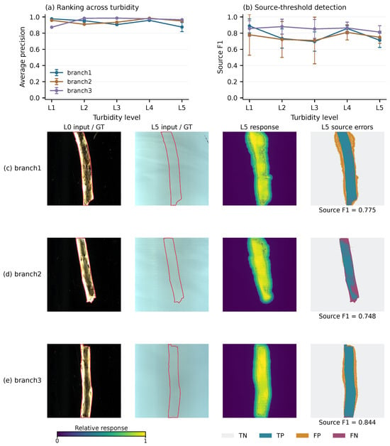
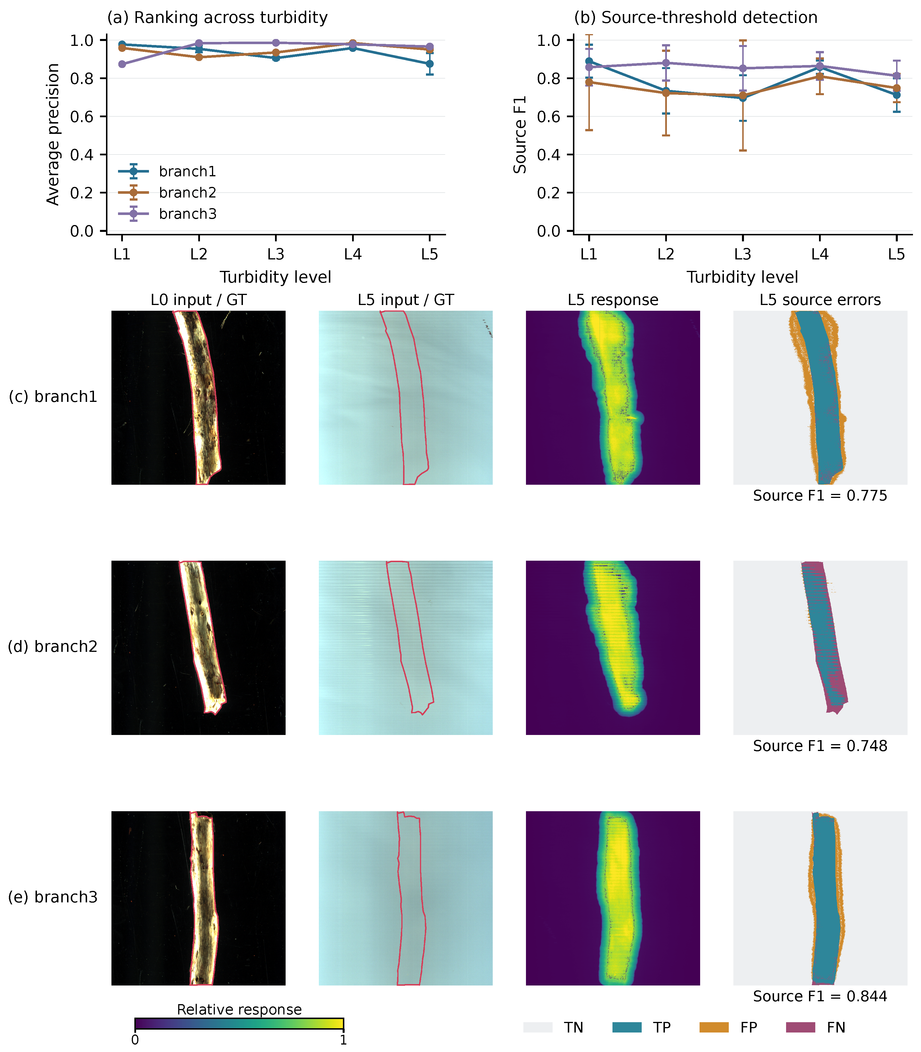
Figure 14 shows responses concentrated around all three wooden targets, together with residual background and missed boundary pixels. These full-field examples complement the five-seed summaries in Table 6.

Figure 14. Wooden-target AP and Source F1 across levels (a,b), with full-field L0/L5 inputs, L5 responses, and source-threshold errors for branch1–branch3 (c–e; seed 36). Curves show five-seed means ± sample SD. RGB bands are 649.33/549.45/470.00 nm. Red contours denote references; normalized response colors are for display only; errors use native scores and frozen L0 thresholds.

4.6.2. Evaluation Under Altered Illumination Directions

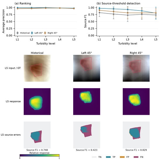
Brick1 maintained mean AP of 0.9927 and 0.9713 under left- and right-rotated illumination, respectively (Table 7). Figure 15 shows the retained target responses and remaining source-threshold errors. Each condition used its own newly acquired L0 source, supporting adaptation after a lighting change rather than frozen-detector invariance. The historical original-direction sequence is a reference, not a same-batch control.

Table 7. Brick1 under historical and left/right 45° lamp-head orientations.

Target	Condition	Overall AP	Overall AUROC	Overall Source F1	L5 AP	L5 Source F1
brick1	Historical	0.9772 ± 0.0015	0.9966 ± 0.0002	0.7606 ± 0.1709	0.9646 ± 0.0027	0.7344 ± 0.1382
brick1	Left 45°	0.9927 ± 0.0001	0.9986 ± 0.0000	0.9081 ± 0.1016	0.9798 ± 0.0004	0.8009 ± 0.2123
brick1	Right 45°	0.9713 ± 0.0009	0.9956 ± 0.0001	0.8372 ± 0.1466	0.9687 ± 0.0009	0.8105 ± 0.1433

Five-seed means ± sample SD. Overall averages L1–L5. Each condition uses its own L0 source, prior, and common-subset threshold; conditions are repeated observations of one physical target.

Figure 15. Brick1 under original, left 45°, and right 45° lamp-head orientations. (a,b) AP and Source F1 across L1–L5, with five-seed means ± sample SD. Lower rows show full-field L5 inputs, relative responses, and source-threshold errors (seed 36). Each condition has its own L0 calibration; original-direction data are historical references. Red contours indicate the target reference boundaries used for evaluation. Display conventions follow Figure 14.

Source-threshold detection showed greater variability across seeds, with an L5 Source F1 of $0.8009\pm 0.2123$ under left-rotated illumination (Table 7). The displayed seed 36 case yielded a Source F1 of 0.423 (Figure 15), illustrating the difference between individual examples and five-seed summaries.

Together, the wooden-target and brick1 illumination results extend the tested materials and lighting directions under target-specific training and adaptation. They do not establish zero-shot recognition or invariance to arbitrary environmental changes.

4.7. Error Propagation Under Early-Stage Pseudo-Anchor Perturbations

We examined early-error propagation on four physical-target sequences spanning brick and stone (brick1, brick2, stone1, and stone2) using seeds 36–40. In each L1 pseudo-anchor update round, 10% or 20% of the pseudo-anchor labels were randomly selected within each pseudo-anchor class and flipped. L2–L5 then followed the normal order, inheriting adapted states and response memory. Historical clean controls were paired by target, seed, and level. Evaluation used CTP-DA responses before RG-OBS, with target-domain labels reserved for offline assessment. Source F1 used a threshold calibrated on native L0 scores from the common subset of 180 target and 180 background pixels, without scene normalization; this threshold was fixed across L1–L5 and paired conditions. At each level, we calculated the clean-minus-perturbed metric difference as

$$\Delta {\mathcal{V}}_l={\mathcal{V}}_l^{\mathrm{clean}}-{\mathcal{V}}_l^{\mathrm{perturbed}},$$

(63)

where $\mathcal{V}$ denotes AP, AUROC, or Source F1; positive differences indicate lower performance after perturbation.

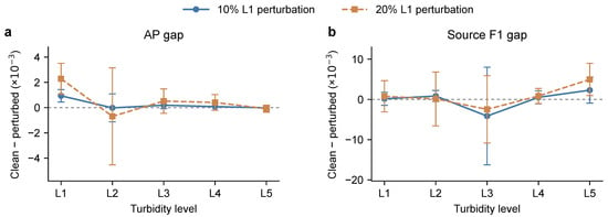
Mean ranking differences did not show sustained growth across levels (Figure 16a). L1 AP gaps were 0.000937 and 0.002285 for 10% and 20% perturbations, respectively. Although signed differences fluctuated at intermediate levels, the magnitudes of their means remained below the L1 gaps and approached zero at L5, reaching −0.000015 and −0.000084. AUROC gaps likewise narrowed from 0.001877 and 0.005847 at L1 to absolute values below 0.00001 at L5. Terminal AP was 0.948449 ± 0.001130 for the clean control, 0.948464 ± 0.001126 for 10% perturbation, and 0.948533 ± 0.001105 for 20% perturbation. Initial effects varied across targets and seeds, with the largest mean L1 AP loss in stone2.

Figure 16. Early-stage pseudo-anchor perturbation effects across turbidity levels. Clean-minus-perturbed differences in (a) AP and (b) Source F1 are shown for 10% and 20% L1 pseudo-anchor label perturbations. Points and error bars denote means ± sample SD across five seeds (36–40), after equal averaging over four targets within each seed. Differences are displayed in units of ${10}^{-3}$; dashed horizontal lines mark zero. Responses precede RG-OBS.

Fixed-source-threshold detection retained small residual mean differences (Figure 16b). L5 Source F1 was 0.713350 ± 0.052657 for the clean control, 0.711056 ± 0.050983 for 10% perturbation, and 0.708383 ± 0.050397 for 20% perturbation, corresponding to mean reductions of 0.23 and 0.50 percentage points. Within these four target sequences and the tested 10% and 20% L1 perturbations, CTP-DA maintained terminal ranking performance close to the clean control, while small Source F1 differences persisted.

4.8. Computational Efficiency and Online Adaptation Cost

Computational costs were measured on an Intel Core i7-14700HX CPU and an NVIDIA RTX 4070 Laptop GPU. Profiling used brick1–brick3 and stone1–stone3 at L1, L3, and L5 (18 scenes; seed 37), with 800 × 800 × 181 inputs. Each case used one warm-up and three timed repetitions; neural inputs were FP32 with pixel or patch batches of 1024. Detection time covered a CPU-resident cube through to a CPU-resident continuous response map, including data transfers and response processing. Disk and model loading, iterative fitting or adaptation, metric calculation, and export were excluded; MF and CEM scene-statistic estimation remained within this boundary.

The profiling subset comprises two representative classical detectors, MF and CEM, and all six evaluated neural network implementations, including Full (Table 8A). All neural networks were timed with fitted or adapted states held fixed; TSDA test-time updates and Full’s adaptation and auxiliary-network fitting were excluded.

Table 8. Computational costs under separately defined measurement scopes. (A) Original eighteen-scene post-fit detection benchmark. (B) Additional four-case resource checks for brick1 and stone1 at L1/L5, seed 37.

(A) Original Eighteen-Scene Detection Benchmark
Method	Network Parameters (K)		Network GFLOPs/Cube	Detection Time  (s/cube)		Peak Allocated GPU Memory (MiB)
MF	—		—	2.16 ± 0.18		— (CPU)
CEM	—		—	1.83 ± 0.05		— (CPU)
NUN-UTD	73.271		92.98	1.14 ± 0.02		455.99
SVHAE	66.935		21.55	1.08 ± 0.08		454.39
HUTDNet-based	603.682		58,973.54	9.35 ± 0.19		707.77
DANN	21.274		26.06	1.04 ± 0.09		455.70
TSDA	809.759		66,870.00	47.67 ± 0.60		2115.30
Full	164.977		300.56	30.49 ± 2.35		176.05
(B) Additional four-case resource checks
Method	Batch 1 time case-mean range (s)	Recheck time (s) mean ± between-case SD	Recheck cubes/min	Recheck CPU WS/private (GiB)	Recheck GPU (MiB)	Sampled GPU board energy (J)
Full	31.41–223.43	49.20 ± 34.35	1.22	4.21 / 6.46	176.05	135.76–158.66
NUN-UTD	1.23–11.93	5.87 ± 5.47	10.22	1.73 / 2.72	455.99	13.48–52.37
MF	2.17–2.38	2.02 ± 0.03	29.75	2.69 / 3.05	NA	NA

(A) Network parameters include all loaded detector-network parameters, including retained auxiliary branches; training-only networks and non-network state are excluded. Network GFLOPs count executed Linear/Conv operations (1 MAC = 2 FLOPs), excluding other operators and CPU processing; they are not whole-pipeline FLOPs. Detection times are means ± sample standard deviations across 18 scene means, each averaged over three repetitions. GPU memory is the maximum PyTorch (2.10.0+cu126 (CUDA 12.6)) allocation across scenes, excluding CPU memory and GPU reservations. Dashes indicate non-network quantities or CPU-only execution. The bold method name identifies Full; numerical values are not bolded. (B) Batch 1 is the earlier post-warm-up benchmark, not cold-start timing. Ranges and sample SD summarize four case means. Throughput is 60/mean recheck time. CPU values are sampled maximum working set/private commit (GiB); GPU values are peak allocation. Recheck GPU-board energy uses trapezoidal integration of NVML power over each separate sampling call (nominal 0.1 s polling), without idle subtraction. GPU-board energy is inapplicable to CPU-only MF; its CPU energy was not measured. For Full/brick1/L5, the energy call lasted 33.25 s (158.66 J), separate from formal calls of 29.72–153.30 s. Neither batch is pooled with A.

Table 8A places Full between the lightweight spectral models and HUTDNet-based or TSDA in network size and computation. Full required 30.49 ± 2.35 s per cube, approximately 36% less than TSDA, but longer than the other evaluated methods. Its peak allocated GPU memory was 176.05 MiB, the lowest among the evaluated neural network implementations under this configuration.

Online adaptation was measured separately over six complete L1–L5 sequences using seed 37. Across their 30 stages, adaptation, complete detection, and stage-output writing required 120.12 ± 38.71 s per stage (mean ± sample standard deviation). Mean sequence wall time, including sequence preparation and input/output, was 611.45 s (10.19 min), with a maximum allocated GPU memory of 186.17 MiB. These measurements excluded L0 source training and cannot be combined arithmetically with the detection times in Table 8A.

Four-case resource checks (Table 8B) used three warm-ups and three timed calls per case in each batch, with separate sampling and profiling. These checks are distinct from the eighteen-scene Table 8A benchmark. Dedicated profiles gave RG-OBS times of 9.86–15.58 s. Separate 90-stage CTP-DA diagnostics gave mean per-stage times of 44.36 s for response components and 41.61 s for adaptation-round training. These diagnostic timings use a different scope and are not an additive decomposition of Full’s 120.12 s/stage. Caching transforms and reducing redundant candidates are optimization directions. GPU-board energy excludes CPU/system consumption; embedded and real-time deployment remain untested.

5. Discussion

CTP-DA and RG-OBS address complementary problems: maintaining target–background ranking and suppressing spatial background expansion after adaptation. Reliability weighting, spatial memory, and spectral contrast provided the strongest internal ranking evidence. Matched-input controls support complete RG-OBS calibration without establishing that every auxiliary operation is individually necessary.

High AP can coexist with imperfect L0 threshold transfer and weak boundary responses. Boundary agreement also depends on transferred-mask uncertainty; the gradient-support shifts are not independent registration residuals. Mask perturbations assess reference sensitivity, while independent target annotations and held-out source calibration would strengthen operating-point validation.

The target-specific L0 reference limits unknown-target detection, which would require discovery or reference initialization. Area-prior and risk-threshold perturbations assess calibration uncertainty, rather than physical size, pose, or position changes. Confidence-guided scale updates remain a possible extension requiring target-preservation checks.

The prescribed L0–L5 order follows cumulative kaolin addition. The evidence is strongest for controlled, approximately fixed-geometry sequences with a clear-water reference; arbitrary dynamic or nonmonotonic domain transitions require further validation. Natural water, dynamic flow, camera motion, nonuniform illumination, and shared multi-object detection require further evaluation. Architectural and training-budget differences limit cross-system causal attribution; matched internal controls provide more direct module evidence. The implemented baselines do not exhaust recent underwater or source-free/continual methods. Early-error propagation and desktop costs are examined in Section 4.7 and Section 4.8; real-time and embedded deployment remain untested.

6. Conclusions

We developed a target-specific underwater hyperspectral detector that combines progressive domain adaptation with risk-gated background suppression. On the controlled cross-turbidity benchmark, the complete framework achieved AP = 0.9282 ± 0.0009 and common-L0 Source F1 = 0.7750 ± 0.0236. Controlled ablations linked these gains to complementary improvements in target–background ranking and spatial background calibration. Additional wooden-target and altered-illumination evaluations extended the tested material and lighting conditions, with each sequence using its own labeled L0 reference and target prior. The results support adapting through intermediate unlabeled domains while constraining the final response with reliable object evidence. Broader geometric variation, independent target-domain annotation, shared multi-target detection, and field deployment remain to be evaluated.

References

- Nashat, M.; Zayed, T. A hybrid review of sewer inspection tools and automated CCTV image analysis techniques. Undergr. Space 2025, 25, 295–326. [Google Scholar] [CrossRef] [Scilit]
- Lechevallier, P.; Villez, K.; Felsheim, C.; Rieckermann, J. Towards non-contact pollution monitoring in sewers with hyperspectral imaging. Environ. Sci. Water Res. Technol. 2024, 10, 1160–1170. [Google Scholar] [CrossRef] [Scilit]
- Akkaynak, D.; Treibitz, T. A revised underwater image formation model. In Proceedings of the 2018 IEEE/CVF Conference on Computer Vision and Pattern Recognition (CVPR), Salt Lake City, UT, USA, 18–22 June 2018; pp. 6723–6732. [Google Scholar] [CrossRef] [Scilit]
- Kruse, F.A.; Lefkoff, A.B.; Boardman, J.W.; Heidebrecht, K.B.; Shapiro, A.T.; Barloon, P.J.; Goetz, A.F.H. The spectral image processing system (SIPS)—Interactive visualization and analysis of imaging spectrometer data. Remote Sens. Environ. 1993, 44, 145–163. [Google Scholar] [CrossRef] [Scilit]
- Chang, C.I.; Ren, H.; Chiang, S.S. Real-time processing algorithms for target detection and classification in hyperspectral imagery. IEEE Trans. Geosci. Remote Sens. 2001, 39, 760–768. [Google Scholar] [CrossRef] [Scilit]
- Kraut, S.; Scharf, L.L.; McWhorter, L.T. Adaptive subspace detectors. IEEE Trans. Signal Process. 2001, 49, 1–16. [Google Scholar] [CrossRef] [Scilit]
- Robey, F.C.; Fuhrmann, D.R.; Kelly, E.J.; Nitzberg, R. A CFAR adaptive matched filter detector. IEEE Trans. Aerosp. Electron. Syst. 1992, 28, 208–216. [Google Scholar] [CrossRef] [Scilit]
- Harsanyi, J.C.; Chang, C.I. Hyperspectral image classification and dimensionality reduction: An orthogonal subspace projection approach. IEEE Trans. Geosci. Remote Sens. 1994, 32, 779–785. [Google Scholar] [CrossRef] [Scilit]
- Jay, S.; Guillaume, M.; Blanc-Talon, J. Underwater target detection with hyperspectral data: Solutions for both known and unknown water quality. IEEE J. Sel. Top. Appl. Earth Obs. Remote Sens. 2012, 5, 1213–1221. [Google Scholar] [CrossRef] [Scilit]
- Fu, X.; Shang, X.; Sun, X.; Yu, H.; Song, M.; Chang, C.I. Underwater hyperspectral target detection with band selection. Remote Sens. 2020, 12, 1056. [Google Scholar] [CrossRef] [Scilit]
- Qi, J.; Gong, Z.; Yao, A.; Liu, X.; Li, Y.; Zhang, Y.; Zhong, P. Bathymetric-based band selection method for hyperspectral underwater target detection. Remote Sens. 2021, 13, 3798. [Google Scholar] [CrossRef] [Scilit]
- Qi, J.; Wan, P.; Gong, Z.; Xue, W.; Yao, A.; Liu, X.; Zhong, P. A self-improving framework for joint depth estimation and underwater target detection from hyperspectral imagery. Remote Sens. 2021, 13, 1721. [Google Scholar] [CrossRef] [Scilit]
- Li, Z.; Li, J.; Zhang, P.; Zheng, L.; Shen, Y.; Li, Q.; Li, X.; Li, T. A transfer-based framework for underwater target detection from hyperspectral imagery. Remote Sens. 2023, 15, 1023. [Google Scholar] [CrossRef] [Scilit]
- Pálsson, B.; Sveinsson, J.R.; Úlfarsson, M.Ö. Blind hyperspectral unmixing using autoencoders: A critical comparison. IEEE J. Sel. Top. Appl. Earth Obs. Remote Sens. 2022, 15, 1340–1372. [Google Scholar] [CrossRef] [Scilit]
- Qi, J.; Gong, Z.; Xue, W.; Liu, X.; Yao, A.; Zhong, P. An unmixing-based network for underwater target detection from hyperspectral imagery. IEEE J. Sel. Top. Appl. Earth Obs. Remote Sens. 2021, 14, 5470–5487. [Google Scholar] [CrossRef] [Scilit]
- Liu, J.; Qi, J.; Zhu, D.; Wen, H.; Jiang, H.; Zhong, P. Detecting nearshore underwater targets with hyperspectral nonlinear unmixing autoencoder. IEEE Trans. Geosci. Remote Sens. 2024, 62, 5529615. [Google Scholar] [CrossRef] [Scilit]
- Li, Q.; Zu, X.; Zhang, M.; Li, J.; Feng, Y. HUTDNet: A joint unmixing and target detection network for underwater hyperspectral imagery. Int. J. Appl. Earth Obs. Geoinf. 2025, 136, 104374. [Google Scholar] [CrossRef] [Scilit]
- Liu, M.; Zhong, S. NCSS-Net: A negatively constrained network with self-supervised band selection for hyperspectral image underwater target detection. Remote Sens. 2026, 18, 418. [Google Scholar] [CrossRef] [Scilit]
- He, Y.; Wang, H.; Li, B.; Zhao, H. Gradual domain adaptation: Theory and algorithms. J. Mach. Learn. Res. 2024, 25, 1–40. Available online: https://jmlr.org/papers/v25/23-1180.html (accessed on 16 July 2026).
- Chen, H.Y.; Chao, W.L. Gradual domain adaptation without indexed intermediate domains. In Proceedings of the Advances in Neural Information Processing Systems; Ranzato, M., Beygelzimer, A., Dauphin, Y., Liang, P., Vaughan, J.W., Eds.; Curran Associates, Inc.: Red Hook, NY, USA, 2021; Volume 34, pp. 8201–8214. Available online: https://proceedings.neurips.cc/paper/2021/hash/45017f6511f91be700fda3d118034994-Abstract.html (accessed on 16 July 2026).
- Gerster, R.; Stütz, P. Towards robust hyperspectral target detection via test-time spectrum adaptation. Remote Sens. 2025, 17, 2756. [Google Scholar] [CrossRef] [Scilit]
- Zhang, X.; Gao, K.; Wang, J.; Wang, P.; Hu, Z.; Yang, Z.; Zhao, X.; Li, W. Target detection adapting to spectral variability in multi-temporal hyperspectral images using implicit contrastive learning. Remote Sens. 2024, 16, 718. [Google Scholar] [CrossRef] [Scilit]
- Zhang, W.; Hu, R.; Wang, J.; Zhang, L.; Zhu, C. Spectral prototype attention domain adaptation for hyperspectral image classification. Remote Sens. 2025, 17, 3901. [Google Scholar] [CrossRef] [Scilit]
- Wang, X.; Wang, L.; Wang, Q.; Vizziello, A.; Gamba, P. Hyperspectral target detection via global spatial–spectral attention network and background suppression. IEEE J. Sel. Top. Appl. Earth Obs. Remote Sens. 2023, 16, 9011–9024. [Google Scholar] [CrossRef] [Scilit]
- Yang, L.; Song, X.; Bai, B.; Chen, Z. Adaptive background endmember extraction for hyperspectral subpixel object detection. Remote Sens. 2024, 16, 2245. [Google Scholar] [CrossRef] [Scilit]
- Ali, M.K.; Amin, B.; Maud, A.R.; Bhatti, F.A.; Sukhia, K.N.; Khurshid, K. Hyperspectral target detection using self-supervised background learning. Adv. Space Res. 2024, 74, 628–646. [Google Scholar] [CrossRef] [Scilit]
- Li, H.; Li, L.; Wang, H.; Zhang, W.; Liu, J.; Ren, P. Joint underwater image enhancement and captioning through multisupervised chained task learning. IEEE Trans. Geosci. Remote Sens. 2026, 64, 4209622. [Google Scholar] [CrossRef] [Scilit]
- Li, H.; Li, L.; Wang, H.; Zhang, W.; Ren, P. Large foundation model empowered region-aware underwater image captioning. Int. J. Comput. Vis. 2026, 134, 66. [Google Scholar] [CrossRef] [Scilit]
- Zhao, M.; Wang, M.; Chen, J.; Rahardja, S. Hyperspectral unmixing for additive nonlinear models with a 3-D-CNN autoencoder network. IEEE Trans. Geosci. Remote Sens. 2022, 60, 5509415. [Google Scholar] [CrossRef] [Scilit]
- Nascimento, J.M.P.; Bioucas-Dias, J.M. Vertex component analysis: A fast algorithm to unmix hyperspectral data. IEEE Trans. Geosci. Remote Sens. 2005, 43, 898–910. [Google Scholar] [CrossRef] [Scilit]
- Tarvainen, A.; Valpola, H. Mean teachers are better role models: Weight-averaged consistency targets improve semi-supervised deep learning results. In Proceedings of the Advances in Neural Information Processing Systems; Guyon, I., von Luxburg, U., Bengio, S., Wallach, H., Fergus, R., Vishwanathan, S.V.N., Garnett, R., Eds.; Curran Associates, Inc.: Red Hook, NY, USA, 2017; Volume 30, pp. 1195–1204. [Google Scholar]
- Aala, S.; Kumar Sikhakolli, S.; Chinnadurai, S.; Deshpande, A.; Elumalai, K.; Sarker, M.A.L.; Mostafa, H. SVHAE: Spectral variability-aware hybrid autoencoder for hyperspectral underwater target detection. IEEE Access 2025, 13, 129161–129171. [Google Scholar] [CrossRef] [Scilit]
- Ganin, Y.; Ustinova, E.; Ajakan, H.; Germain, P.; Larochelle, H.; Laviolette, F.; Marchand, M.; Lempitsky, V. Domain-adversarial training of neural networks. J. Mach. Learn. Res. 2016, 17, 1–35. Available online: https://www.jmlr.org/papers/v17/15-239.html (accessed on 17 October 2026).
- Fang, Z.; He, Y.; Li, Z.; Gong, X. Two-stage domain adaptation for hyperspectral image classification based on self-distillation and test-time adaptation. IEEE Geosci. Remote Sens. Lett. 2025, 22, 5504405. [Google Scholar] [CrossRef] [Scilit]
Disclaimer/Publisher’s Note: The statements, opinions and data contained in all publications are solely those of the individual author(s) and contributor(s) and not of MDPI and/or the editor(s). MDPI and/or the editor(s) disclaim responsibility for any injury to people or property resulting from any ideas, methods, instructions or products referred to in the content. |
© 2026 by the authors. Licensee MDPI, Basel, Switzerland. This article is an open access article distributed under the terms and conditions of the Creative Commons Attribution (CC BY) license.