


Highlights
What are the main findings?
- UniRS-Seg unifies semantic and referring remote sensing segmentation in one adapted SAM ViT-B + SigLIP 2 model with a shared, query-conditioned mask decoder.
- It achieves the highest listed mIoU/gIoU on six benchmarks: 57.30% (LoveDA), 85.31% (Vaihingen), 88.24% (Potsdam), 78.18% (RefSegRS), 70.88% (RRSIS-D), and 72.91% (RISBench).
What are the implications of the main findings?
- A common query-conditioned decoder supports both task families; the joint-training comparison improves the reported mean metrics over the single-task controls.
- Joint task-balanced training with cross-modal consistency yields positive transfer between semantic and referring segmentation, supporting unified segmentation pipelines for Earth observation.
Abstract
Remote sensing semantic and referring segmentation share mask geometry but differ in whether a category vocabulary or a natural-language expression selects the output. UniRS-Seg bridges these interfaces through a shared sparse–dense query compiler and a hierarchical mask decoder, jointly trained on independently annotated datasets. Class names and referring expressions are projected from SigLIP 2 into the same decoder space; dense image–query activations supply spatial support, and sparse query tokens specify the requested region. An adapted SAM ViT-B pathway and parallel convolutional features recover local geometry, while learnable soft mask cross-attention refines both tasks and class-balanced mask-guided self-attention supports semantic parsing. UniRS-Seg achieves 57.30%, 85.31%, and 88.24% mIoU on LoveDA, Vaihingen, and Potsdam, and 78.18% and 70.88% gIoU on RefSegRS and RRSIS-D. These scores exceed the strongest listed baseline means by 0.68, 0.99, 1.18, 0.79, and 1.71 percentage points, respectively. Against separately trained semantic-only and referring-only versions of the shared architecture, joint training improves the four evaluated datasets by 0.45, 0.89, 1.40, and 0.97 points. An additional supervised RISBench evaluation achieves 72.91% gIoU and 74.85% cIoU, with the highest gIoU among the listed methods. On RefSegRS, adding learnable mask cross-attention to combined sparse and dense prompts increases gIoU by 0.86 points. The results support supervised dual-task transfer through a common query-conditioned decoder; the comparison uses published baseline results and does not establish unseen-domain or zero-shot generalization.
1. Introduction
Pixel-level remote sensing interpretation must recover both the category and spatial extent of geospatial regions. Semantic segmentation labels every pixel using a predefined land-cover vocabulary, whereas referring segmentation extracts the region selected by a natural-language expression. These interfaces are useful for complementary operations: mapping all buildings in a scene and isolating the building described relative to a road, for example. Both depend on geometry that is difficult in overhead imagery, including densely repeated small objects, large scale variation, irregular vegetation, low-contrast boundaries, and shadows [1]. Training two independent pipelines duplicates the adaptation and boundary-recovery machinery even though the outputs are masks of related scene content.
Recent semantic methods address global context and local detail with Transformer and state-space designs, including UNetFormer, RS3Mamba, UNetMamba, and PyramidMamba [2,3,4,5]. Attention-enhanced segmentation also uses cross-region and channel interactions to preserve small objects and boundaries [6]. In the semisupervised setting, APRW combines adaptive patch augmentation (APA) with class ranking weights to address perturbation diversity and imbalance [7]. These advances concern visual representation or supervision, but do not directly connect exhaustive land-cover prediction to expression-conditioned selection. Conversely, RefSegRS and RRSIS-D establish language-guided overhead segmentation benchmarks [8,9]; RMSIN emphasizes rotated multi-scale interaction, and FIANet improves fine-grained image–text alignment [9,10]. Their referring masks remain distinct from a full-scene semantic labeling interface.
Foundation models offer complementary priors for connecting the tasks. SAM supplies prompt-conditioned mask geometry, while adapters help bridge the natural-image/overhead-image gap [11,12,13]. RemoteCLIP and SigLIP 2 strengthen image–text representations, and SkySense supports broad Earth-observation interpretation [14,15,16]. RSRefSeg, RS2-SAM2, and RSRefSeg 2 combine vision–language localization with SAM-family segmentation [17,18,19]. Unification itself is also an active direction: UniGeoSeg extends instruction-driven geospatial segmentation across referring, interactive, and reasoning tasks [20]. Thus, neither combining foundation models nor pursuing several segmentation interfaces is by itself a sufficient novelty claim.
The question addressed here is more specific: can a class-vocabulary query bank and a free-form expression use the same sparse–dense interface and mask decoder, and does joint supervision improve both task families? A fixed semantic classifier is tied to one taxonomy, whereas an expression decoder must discriminate instances using attributes and relations. Sharing their weights can transfer category and contour evidence, but can also introduce conflicts between exhaustive class coverage and selective instance extraction. Independently annotated datasets further prevent assuming that every image has both forms of supervision. The architecture and training scheme must therefore connect compatible signals without inventing referring annotations from semantic labels.
We propose UniRS-Seg to address this gap. SigLIP 2 encodes dataset class names or a referring expression in a common query space. Query-to-patch similarities generate a dense spatial prompt, and activation-weighted visual pooling forms a sparse mask token. Both condition an adapted SAM ViT-B pathway with convolutional detail recovery and one hierarchical decoder. Learnable mask cross-attention uses the current soft prediction as a spatial prior; semantic-mode class-balanced attention reduces majority-class dominance. Semantic masks support conservative class-union expressions during training, while genuine referring annotations supervise expression-specific selection. Task-balanced sampling keeps either annotation family from dominating. Class queries are cached for image-only semantic inference, and referring inference accepts an expression without manual point or box prompts. The scope is supervised segmentation over the evaluated taxonomies, rather than zero-shot recognition of unseen categories.
The contributions are:
- A shared sparse–dense query interface and dynamic mask decoder that support both full-scene semantic parsing and expression-conditioned remote sensing segmentation.
- Complementary geometry and language pathways, with soft mask attention, semantic class balancing, and hierarchical reconstruction for overhead imagery.
- Annotation-compatible joint training with task-balanced sampling, cross-modal alignment, and class-union consistency, evaluated against separate and single-task controls.
- Evaluation on three semantic and three referring benchmarks, including an additional supervised RISBench experiment, with component, prompt, confidence, augmentation, training-regime, and adaptation ablations, corruption analysis, and measured computational profiling.
2. Related Work
2.1. Remote Sensing Semantic Segmentation
Fully convolutional networks established end-to-end dense prediction by replacing fully connected layers with spatial classifiers [21]. U-Net popularized symmetric encoder–decoder processing and skip connections for recovering high-resolution structure [22]. Atrous convolution and pyramid pooling subsequently enlarged receptive fields without proportionally reducing output resolution [23]. These ideas are particularly relevant in remote sensing, where a single tile may contain compact cars, elongated roads, individual roofs, and broad vegetation regions. Transformer models introduced long-range token interaction into segmentation. Swin Transformer provided hierarchical features through shifted-window attention [24]. BANet combined convolutional and Transformer representations for very-fine-resolution urban imagery, DC-Swin introduced a Transformer scheme for fine-resolution segmentation, and UNetFormer combined an efficient encoder with a global–local Transformer decoder [2,25,26]. More recent state-space designs pursue global modeling with approximately linear sequence complexity. RS3Mamba, UNetMamba, UMFormer, PyramidMamba, and PPMamba explore different scan, fusion, and decoder strategies [3,4,5,27,28]. Attention-based alternatives address spatial and channel context explicitly. Tong et al. combine CrossFormer with attention-enhanced multi-scale processing for urban segmentation [6]. APRW uses adaptive patch augmentation and class ranking weights in semisupervised segmentation [7]; its unlabeled-data and pseudo-label setting differs from the supervised dual-task protocol used here. WASP-Mamba combines multi-scale state-space aggregation with frequency-aware reconstruction and reports results on all three semantic datasets used here [29].
Explicit category modeling provides complementary context. D2LS dynamically refines class embeddings through iterative image–dictionary cross-attention, addressing appearance ambiguity with input-conditioned semantic representations [30]. SA-DDL extends this direction with a spatially adaptive dictionary field, a Local Context Modulator, and a Region-Aware Interaction Decoder [31]. These methods focus on semantic segmentation and local category variation. In contrast, CMAttn uses soft prediction-weighted class prototypes within the semantic branch of a shared semantic/referring decoder; expression-guided inference retains LMCAM while bypassing semantic class balancing. This distinction separates the present task-unification study from dictionary-based semantic representation learning.
Despite these advances, almost all semantic systems retain a dataset-specific output classifier. Changing from LoveDA’s seven labels to the ISPRS taxonomy requires replacing and retraining the classifier. By treating label names as text queries, UniRS-Seg makes the output vocabulary explicit and uses the same dynamic mask generator across taxonomies. This does not automatically make the system open-vocabulary: class performance is still learned from the training taxonomies, and evaluation on unseen categories would require a separate protocol. The benefit claimed here is architectural unification and vocabulary-conditioned decoding, not unmeasured zero-shot recognition.
2.2. Referring Image and Referring Remote Sensing Segmentation
Early referring segmentation models repeatedly fused recurrent language representations with convolutional image features. RRN refined predictions recurrently [32]; CMSA used cross-modal self-attention [33]; BRINet reasoned bidirectionally over relationships [34]; and LSCM modeled linguistic structure [35]. CMPC and its journal extension progressively decomposed and aligned visual and language cues [36,37]. Transformer-based methods strengthened cross-modal context: LAVT injected language into a hierarchical vision Transformer, CRIS exploited CLIP-aligned representations, RIS-DMMI reconsidered one-to-one matching, CARIS modeled context, and CrossVLT divided cross-aware fusion across encoder stages [38,39,40,41,42]. RRSIS adds domain-specific difficulties. RefSegRS contains 4420triplets from 285 aerial scenes and includes categories, attributes, and spatial relations [8,43]. Its language-guided cross-scale enhancement baseline showed the need to combine shallow detail and deep semantics. RRSIS-D, derived from remote sensing visual grounding data, contains 17,402 triplets across 20 categories and substantial scale and rotation variation [9,44]. RMSIN explicitly introduced rotated multi-scale interaction. FIANet decomposes expressions into object and position semantics for finer alignment [10]. More recent methods explore CLIP-driven dynamic feature selection, two-way guidance, and grounding-aware stagewise reasoning [45,46,47]. The common lesson is that language grounding and accurate mask delineation are separable but interdependent. Weak grounding selects the wrong instance, while weak decoding produces incomplete or blurred boundaries even when the instance is localized. UniRS-Seg adopts coarse-to-fine prompting for this reason, but it differs in scope: class-name prompts and referring expressions enter the same prompt interface and mask decoder.
2.3. Segmentation and Vision-Language Foundation Models
SAM consists of a large image encoder, prompt encoder, and lightweight two-way mask decoder [11]. Its promptability and strong boundary prior are attractive for remote sensing, but direct transfer is affected by the gap between ground-view natural images and overhead scenes [13]. SAM-Adapter demonstrated that lightweight trainable modules can inject task-specific information without fully fine-tuning the foundation backbone [12]. Parameter-efficient tuning is especially relevant when combining multiple foundation models. Bottleneck adapters modify activations with small residual modules [48]; LoRA instead parameterizes low-rank weight updates [49]. We use bottleneck adapters to adapt spatial activations while retaining the pretrained SAM weights; Section 5.4 compares this choice with SAM LoRA.
CLIP learned transferable image–text alignment through contrastive supervision [50]. RemoteCLIP and SkySense adapt large-scale multimodal representation learning to Earth observation [14,16]. SigLIP 2 extends sigmoid-loss image–text pretraining with captioning, self-supervised, masked-prediction, and data-curation components; its reported improvements include localization and dense features, making it a suitable interface between text and pixel prediction [15]. We use both its text representations and dense visual tokens. The SigLIP2 image tower supplies semantically aligned localization cues, whereas SAM supplies segmentation-oriented geometry. A learned fusion layer aligns their dimensions and resolutions; the two encoders are not assumed to be natively interchangeable.
Foundation-model RRSIS is a rapidly moving area. EVF-SAM performs early vision-language fusion for text-prompted SAM [51]. RSRefSeg employs CLIP activations as SAM prompts [17]. RS2-SAM2 jointly encodes visual and textual inputs, adapts hierarchical features, and generates a pseudo-mask dense prompt [18]. RSRefSeg 2 uses SigLIP 2 and SAM2 to decouple localization from fine segmentation [19]. These studies motivate language-guided foundation-model prompting and establish the relevant prior art. The architectural distinction evaluated by UniRS-Seg is that the same query-conditioned interface can support both full semantic parsing and referring segmentation while reusing an adapted SAM1 detail-recovery path.
2.4. Universal Segmentation and the Remaining Gap
Mask-classification decoders, exemplified by Mask2Former, represent segmentation as a set of learned queries and masks [52]. This view unifies semantic, instance, and panoptic segmentation more naturally than a fixed pixel classifier. Referring segmentation also produces a query-specific mask, but its query originates in language rather than a learned object slot. UniRS-Seg connects these views by treating a semantic vocabulary as multiple text queries and a referring expression as one text query. The decoder always predicts masks conditioned on query embeddings; task-specific post-processing determines whether the outputs are normalized across classes or thresholded as one binary mask. UniGeoSeg addresses a broader instruction-driven setting with referring, interactive, and reasoning segmentation [20]. CrossEarth uses multi-task training for remote sensing domain generalization [53]. UniRS-Seg instead evaluates supervised semantic/referring transfer through a shared foundation-model prompt interface. A shared model can benefit from complementary supervision or suffer negative transfer between class coverage and instance discrimination. The reported controls therefore compare single-task training, two task-specific models, task-balanced shared training, and shared training with consistency. They assess the present supervised setting rather than replacing a cross-domain evaluation.
3. Materials and Methods
3.1. Problem Formulation
Let denote an optical remote sensing image. In semantic mode, a dataset supplies a vocabulary and a dense label map . The desired output is a set of C logit maps whose pixel-wise softmax gives the semantic prediction. In referring mode, the input additionally contains an expression and the target is a binary mask . Rather than defining two output heads, we express both inputs as a query set Q. Semantic mode contains one query per class name; referring mode contains one query representing the expression, accompanied by its token-level context.
This abstraction separates three concerns. The visual pathway answers what geometric and semantic evidence exists in the image. The query pathway states which classes or described instance should be extracted. The shared decoder maps their interaction to masks. Dataset taxonomies can therefore differ in size without changing the decoder weights. All classes, including LoveDA background and ISPRS clutter/background, remain explicit during training; evaluation may omit a class only when the established benchmark protocol does so.
3.2. Architecture Overview
Figure 1 summarizes UniRS-Seg. The image is processed by two complementary foundation pathways. The adapted SAM1 branch supplies segmentation-oriented tokens and multi-level spatial features. A lightweight CNN in parallel retains high-frequency texture and feeds cross-branch attention. The SigLIP 2 image tower supplies dense vision-language features aligned with the text tower. The text input is either a prompt ensemble built from semantic class names or a free-form referring expression. A query compiler projects both forms into a common decoder space. The two foundation pathways are detailed in Section 3.3, Section 3.4, Section 3.5, Section 3.6 below.
Figure 1.
Overall architecture of UniRS-Seg. The gray block denotes the image; blue denotes the adapted SAM encoder; orange denotes the local CNN; purple denotes SigLIP 2, query/prompt construction, and the referring-mask output; green denotes class-name inputs and the semantic-map output. Teal blocks denote cross-branch attention (CBA) and the shared mask/pixel decoder, including LMCAM. Semantic class names and referring expressions provide the two task interfaces to the shared query-conditioned decoder.
The shared prompt interface performs query-to-image matching on the SigLIP 2 grid. It returns a coarse dense activation prompt and a sparse query token for every requested mask. These prompts condition a generalized SAM mask decoder. Learnable mask cross-attention (LMCAM) uses the current coarse probability as a differentiable spatial prior rather than a hard gate. In semantic mode, class-balanced mask-guided self-attention (CMAttn) further refines image embeddings with soft class prototypes while compensating for the long-tailed pixel distribution. Finally, the hierarchical pixel decoder combines decoder states, intermediate SAM features, and CNN features to recover thin objects and boundaries. Semantic mode runs the query set in parallel and applies a pixel-wise softmax; referring mode applies a sigmoid to one mask.
3.3. SAM Domain Adaptation and Local-Detail Pathway
3.3.1. Bottleneck Adapters
The SAM ViT-B image encoder contains 12 Transformer blocks. Its pretrained weights are frozen by default, and a residual bottleneck adapter is inserted after the attention and feed-forward sublayers of each block. For a token tensor at block k, the adapter update is
Tokensare rows of ; reduces channels and restores them. The scalar is a learnable residual scale initialized near zero. Unlike a prompt vector shared across spatial locations, this adapter transforms each token and can learn remote-sensing-specific appearance while preserving the pretrained backbone at initialization. The bottleneck ratio is 1:4. The adaptation ablation compares this configuration with frozen SAM and SAM LoRA; it does not include a bottleneck-ratio sweep or full fine-tuning.
Features are retained from blocks 3, 6, 9, and 12. Layer normalization and projections map these tensors to a common pyramid width before hierarchical decoding. Retaining intermediate features is necessary because the final SAM grid alone is too coarse for cars, narrow roads, roof outlines, and thin vegetation boundaries.
3.3.2. Parallel CNN and Cross-Branch Attention
The parallel convolutional branch contains a stem followed by four stages at strides 2, 4, 8, and 16. Each stage uses depthwise separable convolutions, normalization, GELU, and residual connections. The branch is intentionally lightweight: its role is to preserve local contrast, corners, texture, and boundary frequency rather than duplicate the global encoder. The stride-16 CNN feature is aligned with the final SAM token grid through learned projections.
Cross-branch attention uses SAM tokens as queries and CNN tokens as keys and values:
where is a relative-position bias and d is the attention width. A feed-forward residual block follows the attention. This direction of attention allows each globally contextual SAM token to retrieve the local evidence most relevant to its location. The lower-resolution CNN stages bypass this module and enter the hierarchical decoder as skip features. Figure 2 illustrates the complete adaptation and detail-recovery pathway.
Figure 2.
SAM domain adaptation and local-detail pathway. Blue blocks denote the frozen SAM ViT-B backbone and features retained from blocks 3, 6, 9, and 12; yellow/orange blocks denote trainable bottleneck adapters, their down–GELU–up residual update, and the lightweight CNN with stride-2/4/8/16 features. The light-blue block denotes cross-branch attention, and the teal block denotes the interface to the hierarchical decoder. SAM tokens supply queries (Q), while aligned CNN features supply keys and values (). Dashed teal arrows carry local skip features to the decoder; gray denotes the input image.
3.4. SigLIP 2 Query Pathway
3.4.1. Dense Visual and Text Representations
The fixed-resolution siglip2-so400m-patch16-512 checkpoint uses separate ViT image and text towers with a shared 1152-dimensional projection space. For a image and a patch size of 16, the vision tower returns unpooled patch tokens. The text tower accepts at most 64 tokens and returns both token-level states and a pooled representation [15]. We denote these outputs by
Here, , , and Pool denotes the checkpoint’s pooled text output used by the query pathway. The pooled image embedding is useful for image–text alignment, but UniRS-Seg retains the unpooled patch states because the dense spatial grid is required for localization. Padding patches introduced by aspect-ratio-preserving preprocessing are excluded with the recorded geometric valid-region mask.
SigLIP 2 retains SigLIP’s pairwise sigmoid objective and augments its pretraining recipe with captioning/localization supervision, self-distillation, and masked-patch prediction. For a batch of B matched image–text pairs, the pairwise component follows the original SigLIP batch normalization [54]:
where hats indicate normalization, t is a learned log-scale, and b is a learned bias. The auxiliary decoder used during SigLIP 2 pretraining is not part of the released encoder. UniRS-Seg therefore uses the released global embeddings and dense hidden states, while its own query compiler and mask decoder learn the remote-sensing task.
3.4.2. Semantic Class Queries
For a semantic dataset, every category name c is inserted into a fixed template set . Examples include “an aerial image of {class}”, “a remote sensing view of {class}”, and “the land-cover class {class}.” If is the mth prompted class string, its query is
where is shared across datasets and is a learned dataset embedding that captures taxonomy-specific label usage, such as the meaning of “background.” Stacking the C vectors gives . These queries are cached after training; consequently, semantic inference requires only the image even though the classifier weights originate from text.
The prompt ensemble makes the classifier vocabulary explicit while avoiding dependence on a single sentence form. It is not used to infer synonyms at evaluation time: benchmark class names and their documented meanings are fixed before training.
3.4.3. Referring Expression Queries
For a referring expression e, the pooled text vector initializes a single query, while token states preserve attributes and relations. A two-layer compiler first attends to the expression tokens and then to the dense image tokens:
Here, SA is token self-attention and is multi-head cross-attention. The first interaction preserves word-level modifiers such as color, size, absolute direction, and relative position; the second makes the final query image-conditioned so that identical language can select different spatial evidence in different scenes. The referring query set is .
3.4.4. Parameter-Efficient VLM Adaptation
The first optimization stage freezes SigLIP 2 and trains only the query compiler and projection layers. The second stage enables low-rank adaptation (LoRA) in the last four image-tower blocks and the last two text-tower blocks. For a frozen projection , the adapted mapping is
with ranks for vision and for text. Only A and B are optimized. Staging the adaptation prevents randomly initialized prompt and decoder layers from immediately perturbing the aligned embedding space. All reported results use the So400m/16 checkpoint at ; smaller checkpoints are treated as distinct model variants rather than silent replacements.
3.5. Shared Sparse–Dense Prompt Interface
Let be the projected SigLIP 2 image grid and let be the jth semantic or referring query. Their normalized similarity yields a coarse activation map
where is a learned log-temperature and is the dense prompt. Only logits used in the spatial softmax are masked to at padded locations; dense-prompt interpolation uses finite activation values and the recorded valid-region geometry. Activation-weighted visual evidence and the sparse prompt token are
where ∥ denotes concatenation and is the positional encoding in the SAM decoder space. We adopt cosine similarity because it decouples the match score from the magnitude of the SigLIP 2 embeddings, so a query’s alignment with a spatial location depends only on directional agreement rather than on feature norm, which can otherwise vary systematically across classes or expressions.
This interface preserves the useful coarse-localization/fine-segmentation decomposition found in foundation-model RRSIS, but it operates identically for C semantic queries or one referring query. In semantic mode the entire class bank is processed in parallel. In referring mode only the expression query is active. The interface does not derive hard points or boxes, avoiding non-differentiable prompt selection and threshold-sensitive failures on small objects.
Figure 3 summarizes the query construction and prompt transfer from SigLIP 2 to the shared decoder.
Figure 3.
SigLIP 2 query and sparse–dense prompt pathway. Purple blocks denote image encoding, the patch grid V, and the expression-query branch; green blocks denote class-name inputs, the cached semantic query bank, and the common query q. The blue block computes query–patch similarity. Teal blocks denote the activation map, upsampling to the dense prompt D, activation-weighted pooling to the sparse token S, and the shared SAM decoder. Gray denotes the input image. Semantic and referring queries use the same prompt-construction operations.
3.6. Query-Conditioned Mask Decoding
3.6.1. Dynamic SAM Mask Tokens
The original SAM mask decoder uses a fixed set of output tokens and hypernetworks. We retain its two-way Transformer initialization but make mask tokens query-conditioned. A shared learned seed is added to a projected query token, yielding one mask token for each active query. Batching these tokens permits a variable number of masks without changing decoder weights. The corresponding hypernetwork maps each decoded query token to channel weights applied to the upsampled image feature. This produces coarse mask logits at one-quarter input resolution.
The decoder also receives the dense prompt through the SAM dense-prompt projection. Consequently, the sparse token carries category or expression semantics, while the dense prompt supplies coarse spatial support. An ablation separates sparse-only, dense-only, and joint prompting.
3.6.2. Learnable Soft Mask Cross-Attention
Hard binary attention masks can suppress a target permanently when an early prediction is wrong. We instead turn the current probability map into a learnable additive bias:
where controls confidence in the mask and prevents numerical singularity. At initialization is small, so cross-attention can recover from poor localization. As training proceeds, the model can use reliable masks to suppress irrelevant regions. This formulation is differentiable everywhere and applies the mask before value aggregation, unlike multiplying an already aggregated attention output.
Figure 4 makes the operation order explicit: the mask is transformed into an additive log-prior before softmax, rather than multiplied onto an already normalized saliency map. For query j and spatial token n, let . Equation (10) gives attention proportional to . For two locations a and b, the attention ratio is
This separates feature compatibility from mask confidence. At the limiting operation is ordinary cross-attention. For , mask contrast is softened; at , the prior is proportional to the current probability; and sharpens preference for already confident locations. Softplus constrains the learned confidence to positive values, with initialization near zero reducing early error reinforcement. A larger weakens the distinction between low-confidence locations, while an excessively small value increases the gradient factor near zero.
Figure 4.
Learnable soft mask cross-attention corresponding to Equation (10). Blue token stacks and the score block denote projected query/image states and feature logits; orange blocks align the predicted soft mask and scale its log-prior by learned confidence; teal circles denote score addition and value aggregation, and the teal rounded block normalizes attention. The mask prior is added to query–key logits before softmax. Gradients pass through both the soft mask and confidence.
The query–key term can confuse repeated roofs or vehicles when appearance is similar. The mask prior can reinforce an incorrect instance or fragment a small target if the initial activation is poor. The learnable confidence adjusts reliance on that prior but does not guarantee recovery from a confidently wrong localization. Value features supply the content used for reconstruction; attention reweighting cannot restore an object absent from those features. The CNN pathway and hierarchical decoder preserve local evidence, while soft masking leaves a recovery path through nonzero attention. These components address different error sources rather than ensuring invariance to occlusion, resolution loss, or unseen scenes.
3.6.3. Class-Balanced Mask-Guided Self-Attention
Remote sensing taxonomies are strongly imbalanced: extensive background, building, or vegetation regions can dominate the features used to refine much smaller classes such as cars and narrow roads. CMAttn is therefore enabled in semantic mode after LMCAM. It uses the decoder’s current soft predictions rather than ground-truth masks, avoiding a train–test mismatch. Let denote image embeddings and the semantic probabilities at the same spatial resolution. For each class, the mask-weighted prototype and dispersion are
Here controls perturbation strength, during training, and is the normalized effective-number weight computed from training-pixel frequency. Squaring, square-root evaluation, and ⊙ act element-wise on channels. The rare-class prototypes consequently receive stronger, variance-aware augmentation. The augmented prototypes are concatenated with the image tokens, processed by self-attention and a feed-forward block, and returned through a gated residual connection. At inference, Gaussian sampling is disabled (), all class queries are retained, and no ground-truth label is required.
In semantic decoding, the same effective-number weights scale cross-entropy and parameterize a learned class-frequency embedding that refines the initial class query from Equation (5). Query dropout affects frequent classes only in auxiliary decoder layers; the final layer always predicts the complete vocabulary. Referring mode has one expression query rather than a semantic class distribution, so it bypasses stochastic class balancing while retaining LMCAM and the shared decoder. Figure 5 illustrates the semantic-mode CMAttn path from mask-guided prototypes to enhanced image embeddings.
Figure 5.
Semantic-mode class-balanced mask-guided self-attention. Blue token stacks denote image embeddings and soft semantic probabilities; orange blocks denote soft-mask pooling, class-frequency weights, and variance-aware prototype perturbation. Teal denotes token concatenation (∥), self-attention/FFN with a gated update, and residual addition (+); the dashed blue path supplies image tokens and the residual. Gaussian sampling is disabled at inference. Soft predictions, rather than ground-truth masks, form the prototypes. Referring inference bypasses this semantic class-balancing path.
3.6.4. Hierarchical Pixel Decoder
The hierarchical pixel decoder reconstructs full-resolution logits in three stages. Starting from the stride-16 decoder feature, it upsamples to strides 8, 4, and 1. Before each concatenation, retained SAM and CNN features are projected and resized to the current decoder grid; they are then combined with the upsampled query-conditioned state. A depthwise separable fusion block and a residual projection refine the result. Auxiliary masks at strides 8 and 4 provide deep supervision; only the full-resolution output is used for reporting.
For semantic mode, the C full-resolution mask logits are stacked and normalized across the query dimension. For referring mode, the single logit map is passed through a sigmoid. In compact notation,
The masks are therefore generated by the same decoder parameters, while output normalization expresses the different task semantics.
3.7. Joint Training Objective
Training alternates task-balanced mini-batches rather than forcing semantic and referring samples into one batch structure. For semantic data, the main losses are class-balanced cross-entropy and multi-class Dice. For referring data, binary cross-entropy and binary Dice supervise the expression mask. A boundary loss compares morphological gradients of prediction and target at a fixed three-pixel radius after resizing to a common evaluation scale. Auxiliary decoder stages receive the same task-appropriate mask losses at lower weight.
Two cross-modal objectives regularize the shared interface. First, masked average visual features are aligned with their class or expression query using an in-batch contrastive loss. Second, each semantic mask produces a conservative template expression of the form “all {class}”; the referring-mode output for that template is constrained to agree with the semantic class probability. This consistency loss is applied only to semantic samples and only to class-union language, so it does not pretend that semantic annotations contain instance-level relations.
The total objective is
Task terms absent from the current sample are set to zero. We use , , , , and in all primary experiments.
3.8. Training and Inference Modes
Training has three stages. Stage 1 freezes both foundation encoders and trains adapters, projections, the CNN branch, prompt interface, and decoder for stable initialization. Stage 2 continues training the SAM adapters and enables the selected SigLIP 2 LoRA blocks. Stage 3 jointly fine-tunes on task-balanced batches with a reduced learning rate and cross-task consistency. Dataset sampling is balanced first by task and then by dataset, preventing the larger RRSIS-D set from dominating RefSegRS and preventing tiled semantic datasets from overwhelming referring data.
At semantic inference, the chosen dataset vocabulary is encoded once and cached. All class queries are decoded in parallel, and each pixel receives the class with maximum probability. At referring inference, the expression is encoded online and one mask is thresholded at 0.5; no point, box, or human correction is used. For large tiles, overlapping sliding-window inference with logit averaging is applied before argmax or thresholding.
4. Experimental Setup
4.1. Datasets
4.1.1. LoveDA
LoveDA contains 5987 high-spatial-resolution images of size pixels from Nanjing, Changzhou, and Wuhan, China [55]. The 2522/1669/1796 image train/validation/test split covers urban and rural domains. Its seven labels are background, building, road, water, barren land, forest, and agriculture. The combination of scene-domain shift, class imbalance, small structures, and visually diverse background makes it suitable for testing both the adapted geometry pathway and vocabulary-conditioned mask queries. We use the official split, train on the training set, select hyperparameters on validation only, and obtain test labels through the official evaluation route. No test image is used for prompt selection or early stopping.
4.1.2. ISPRS Vaihingen
The Vaihingen benchmark contains 33 true orthophoto tiles with an average size of approximately pixels and a ground sampling distance of 9 cm [56]. The imagery provides near-infrared, red, and green channels, DSM data, and labels for impervious surfaces, buildings, low vegetation, trees, cars, and clutter/background. For comparability with the established comparison protocol, we use the common 16/17 tile split:training IDs 1, 3, 5, 7, 11, 13, 15, 17, 21, 23, 26, 28, 30, 32, 34, and 37; test IDs 2, 4, 6, 8, 10, 12, 14, 16, 20, 22, 24, 27, 29, 31, 33, 35, and 38. The IRRG channels are mapped to three input channels. Patches of pixels are extracted with 50% overlap for training; overlapping logits are averaged for tile reconstruction. The five foreground categories are used for the primary mIoU and mF1 comparison, matching the cited table, while clutter/background is still predicted and the present table reports the five-class protocol only.
4.1.3. ISPRS Potsdam
Potsdam comprises 38 georeferenced tiles at 5 cm ground sampling distance and uses the same six labels as Vaihingen [56]. RGB, IRRG, DSM, and normalized DSM products exist, but the primary experiment uses RGB only to match the established comparison protocol.Test IDs are 2_13, 2_14, 3_13, 3_14, 4_13, 4_14, 4_15, 5_13, 5_14, 5_15, 6_13, 6_14, 6_15, and 7_13. Tile 7_10 is excluded because of the documented annotation issue in the comparison protocol; the remaining 23 tiles are used for training. Patch extraction and reconstruction follow the Vaihingen procedure.
4.1.4. RefSegRS
RefSegRS is built on high-resolution SkyScapes aerial scenes and contains 4420 image–expression–mask triplets from 285 scenes [8,43]. The official scene-disjoint split contains 2172 training triplets from 151 scenes, 431 validation triplets from 31 scenes, and 1817 test triplets from 103 scenes. Images are standardized to pixels, and the annotation includes 14 hierarchical categories and five attribute groups. Scene-level separation is preserved to prevent nearly identical crops from leaking across splits. The primary model receives the image at in the SAM branch and in the SigLIP2 branch; the ground-truth mask is resized only with nearest-neighbor interpolation.
4.1.5. RRSIS-D
RRSIS-D was introduced with RMSIN and is derived from the RSVGD remote sensing visual-grounding data [9,44]. It contains 17,402 image–expression–mask triplets over 20 categories, divided into 12,181 training, 1740 validation, and 3481 test samples. Images are represented at pixels and span spatial resolutions from approximately 0.5 to 30 m per pixel. Targets range from small vehicles and windmills to large airports and fields, and many classes occur at arbitrary orientation. For SAM, each image is letterboxed to with a recorded valid-region mask; for SigLIP2 it is resized with aspect-ratio-preserving padding to . Predictions are mapped back to the original grid before metrics are computed.
4.1.6. RISBench
RISBench, introduced with CroBIM, contains 52,472 image–expression–mask triplets built from VRSBench annotations, with imagery originating from DOTA-v2 and DIOR [57,58]. It covers 26 object categories, eight attribute types, image patches, and ground sampling distances of 0.1–30 m. We conduct an additional supervised benchmark experiment using its official training partition and report results on its official test partition. The SAM/SigLIP 2 input sizes and mask restoration follow the referring configuration above. This experiment extends dataset coverage; the original five-benchmark joint-training controls and their checkpoint-selection protocol are retained.
4.2. Data Processing and Augmentation
Image normalization follows the pretrained encoder associated with each branch. The SAM input uses SAM’s pixel mean and standard deviation; the SigLIP 2 input uses the checkpoint processor’s normalization. A single decoded RGB image is transformed into the two resolutions to avoid inconsistent color conversion. Masks always use nearest-neighbor resampling.
Semantic training uses random scale in , random crop, horizontal and vertical flips, and rotations by multiples of 90°. Mild brightness, contrast, and saturation jitter is applied with probability 0.5. Referring training uses photometric jitter and random resize only in the primary protocol. Naive flips or rotations are not used because they would invalidate expressions such as “upper-left building” or “vehicle east of the road.” This distinction preserves annotation validity: a geometric transform changes both the mask and the spatial reference frame of directional language. Semantic geometry augmentation broadens orientation and scale coverage; mild photometric jitter broadens appearance coverage without changing the target. Referring resizing preserves relative position and photometric jitter leaves the expression unchanged. Primary results use this policy; Referring resizing preserves relative position and photometric jitter leaves the expression unchanged. Primary results use this policy; the effect of training without augmentation is evaluated separately in Section 5.
4.3. Evaluation Metrics
For semantic segmentation, we report per-class intersection over union (IoU), mean IoU (mIoU), per-class F1, mean F1 (mF1), and overall pixel accuracy (OA). The primary Vaihingen and Potsdam metrics average the five foreground classes in accordance with the cited comparison source. The reported semantic comparisons use the region metrics above; no additional boundary metric is inferred from the qualitative panels.
For referring segmentation, generalized IoU (gIoU) is the arithmetic mean of per-sample mask IoUs. Cumulative IoU (cIoU) sums intersections over all test samples and divides by the summed unions; it therefore gives larger targets greater influence. Precision at threshold x, denoted Pr@x, is the percentage of samples whose IoU exceeds x, with . The present referring tables report these overlap and threshold metrics; boundary F1 and median IoU are not included. Empty predictions and empty targets follow the official dataset evaluator; no post hoc removal of difficult examples is permitted.
4.4. Implementation Settings
The primary configuration uses SAM ViT-B and siglip2-so400m-patch16-512. New decoder, CNN, adapter, and projection parameters use AdamW with learning rate ; SAM adapters use ; and SigLIP2 LoRA parameters use . Weight decay is 0.01 except for normalization, bias, prompt, and temperature parameters, which use zero decay. Gradients are clipped to a global norm of 1.0. A linear warm-up of 1500 optimizer steps is followed by cosine decay to .
Stage 1 trains newly initialized modules for 30 epochs with both foundation encoders frozen. Stage 2 trains adapters and selected LoRA parameters for 80 epochs. Stage 3 performs task-balanced joint training for 100 epochs at one-tenth of the Stage 2 learning rates. The effective batch size is 4 through gradient accumulation; each optimizer step draws one task, then one dataset within that task, with equal task probability and inverse-square-root dataset-size sampling. Automatic mixed precision uses bfloat16 when supported and float16 otherwise. Gradient checkpointing is enabled for both foundation encoders. We have trained our model on a single RTX 5090 GPU.
Primary models are trained with seeds 0, 1, and 2, and model selection uses the arithmetic mean of normalized validation mIoU on the three semantic datasets and validation gIoU on the two referring datasets. No test metric participates in checkpoint selection. The internal UniRS-Seg configurations follow the same implementation setting. Published baseline values retain their source protocols; they are not described as reruns in this environment.
Computational Complexity
The full UniRS-Seg implementation contains 1140.7 M parameters, including 540.7 M in the vision encoders. Of the full model, 32.1 M parameters are trainable (2.81%); this is a subset of the total, not an additional parameter count. A referring forward pass for one image–expression pair requires 2305.16 GFLOPs with a SAM input and a SigLIP 2 image input. On a single RTX 5090, mean forward-pass latency is 312 ms, with 28.4 GB peak training memory and 14.8 GB peak inference memory. Frozen foundation weights reduce the optimization burden but remain active in the image and expression pathways at inference.
Table 1 compares these measurements with published referring-segmentation statistics from Dong et al., [47]. The 32.1 M trainable count is smaller than the listed baseline counts, while the full parameter count and 2305.16 GFLOPs make the deployment cost explicit. Parameter-efficient adaptation therefore addresses optimization cost rather than eliminating foundation-model inference. The baseline rows retain their source checkpoints, inputs, and profiling environment; the latency values provide published context rather than a common-hardware speed ranking.
Table 1.
Computational statistics for referring segmentation. Baseline measurements are from Dong et al., [47]. UniRS-Seg is profiled for one image–expression pair with SAM and SigLIP 2 inputs; its latency is measured on RTX 5090. M denotes millions of parameters. Best values are shown in bold.
4.5. Comparison Protocol and Provenance
The benchmark splits specified in Section 4 are fixed for all internal UniRS-Seg comparisons and ablations. Checkpoint selection and architecture decisions use validation data, with no test-set retuning. The primary tables compare the corresponding benchmark evaluation partitions; however, published methods retain their original training, validation, and preprocessing choices. Thus, identical sample splits and settings can be asserted for our internal controls, but not independently verified for every source-reported baseline.
Table 2, Table 3 and Table 4 include the comparison reported by WASP-Mamba [29]. These baseline values are interpreted as reported or reproduced in that study rather than as independently rerun results here. Its protocol uses crops or resized inputs with flip-based test-time augmentation; the UniRS-Seg entries use the matched test-time setting. Table 2 additionally includes the published LoveDA results of STAR-Net [59], a Swin-T-based dual-encoder model that fuses global semantic context and local spatial detail for agricultural land-cover parsing. STAR-Net reports 56.62% mIoU, compared with 57.30% for UniRS-Seg, and its row retains the original article’s evaluation setting.
Table 2.
Semantic segmentation results on LoveDA (%). Best values are shown in bold.
Table 3.
Semantic segmentation results on ISPRS Vaihingen (%). mIoU and mF1 average the five foreground classes. Best values are shown in bold.
Table 4.
Semantic segmentation results on ISPRS Potsdam (%). mIoU and mF1 average the five foreground classes. Best values are shown in bold.
Table 5 and Table 6 use the RefSegRS and RRSIS-D test comparisons reported by RSRefSeg 2 [19]. They include original RRSIS methods, natural-image referring baselines retrained for aerial imagery, and foundation-model approaches. The additional RISBench baseline results in Table 7 follow RSRefSeg 2 [19], with each compared method cited individually. Baseline values are retained as source-reported percentages; the UniRS-Seg values are produced by the evaluation protocol described above.
Table 5.
Referring segmentation results on the RefSegRS test set (%). Best values are shown in bold.
Table 6.
Referring segmentation results on the RRSIS-D test set (%). Best values are shown in bold.
Table 7.
Referring segmentation results on the RISBench test partition (%). Baseline results follow RSRefSeg 2 [19]. UniRS-Seg is trained using the official RISBench training partition. Best values among the listed methods are bold.
4.6. Ablation Design
All ablations use the same data splits, seed set, training budget, and input resolution as the primary model unless the varied factor is explicitly named. Architecture components are selected on LoveDA and RRSIS-D validation sets and subsequently checked on Vaihingen and RefSegRS, avoiding test-set selection. The confidence study compares fixed with the full model’s learnable confidence at ; removes the mask prior while retaining ordinary cross-attention. The LoveDA augmentation control varies the training augmentation policy. These studies retain the benchmark splits and evaluation metrics described above.
Cumulative module control. Table 8 isolates the contribution of each architectural group. Variant A receives deterministic class or expression prompts but contains no oracle points or boxes. Adding SAM adapters and the CNN/CBA pathway improves both tasks. The sparse–dense interface produces the largest single gain on RRSIS-D (5.34 gIoU points from C to D), while the decoder-attention group and hierarchical decoder provide further improvements. The LMCAM/CMAttn column enables LMCAM for both tasks and CMAttn for semantic samples only, following Section 3.6.3. Joint training raises the final LoveDA mIoU from 56.98% to 57.30% and RRSIS-D gIoU from 70.01% to 70.88%.
Table 8.
Component ablation on LoveDA and RRSIS-D.
Sparse and dense prompting. Table 9 compares sparse, dense, and joint prompting on RefSegRS. The prompt ablation distinguishes semantic identity from spatial support. Sparse and dense prompts together outperform either input alone. Adding LMCAM to the joint prompt increases RefSegRS gIoU from 77.32% to 78.18%, cIoU from 80.12% to 81.65%, and Pr@0.9 from 34.22% to 35.12%, indicating that soft iterative spatial guidance improves both mean overlap and strict-mask accuracy.
Table 9.
Sparse–dense prompt ablation on RefSegRS.
Joint and task-specific training. Table 10 evaluates the effect of shared training under equal optimizer-step counts. The semantic-only and referring-only controls retain the SAM ViT-B/SigLIP 2 backbone pair, prompt pathway, decoder, input sizes, optimizer settings, augmentation policy, and applicable mask losses; the available task supervision changes. The two task-specific models have independent copies of the corresponding architecture, with no weight sharing or cross-task consistency. This is an accuracy control, not an equal-total-parameter deployment comparison: storing both models duplicates the shared pathways. Equal total optimizer steps also do not imply equal task-specific exposure under alternated joint batches. Relative to semantic-only training, the full model gains 0.45 and 0.89 mIoU points on LoveDA and Vaihingen; relative to referring-only training it gains 1.40 and 0.97 gIoU points on RefSegRS and RRSIS-D. The full model exceeds the two task-specific models by 0.83 and 1.19 mIoU points on LoveDA and Vaihingen and by 1.94 and 1.76 gIoU points on RefSegRS and RRSIS-D. Consistency supervision also improves every dataset relative to task-balanced sampling alone, with gains ranging from 0.12 to 0.67 points.
Table 10.
Joint-training and single-task controls under the fixed benchmark splits and common UniRS-Seg backbone/decoder setting. Metrics are percentages. Dashes indicate that a task is not trained or evaluated by that control.
4.7. Reproducibility
Each experiment stores the dataset version and split, checkpoint identifiers, input processors, class prompt templates, random seed, optimizer groups, learning-rate schedule, loss weights, and software versions. Semantic label mappings are stored in query order, including ignore indices. Referring records retain the exact expression, tokenizer revision, original image size, padding transform, and inverse transform. Metrics are computed from saved per-sample masks rather than copied from training logs.
5. Results
5.1. Semantic Segmentation Performance
The semantic comparison in Table 2, Table 3 and Table 4 includes the source-reported WASP-Mamba comparison [29], with the published STAR-Net result [59] added to Table 2. In Table 2, Bac., Bui., Roa., Wat., Bar., For., and Agr. denote background, building, road, water, barren land, forest, and agriculture, respectively. In Table 3 and Table 4, Imp., Bui., Low., Tre., and Car. denote impervious surface, building, low vegetation, tree, and car; the mean scores average these five foreground categories, and the Potsdam comparison uses RGB input. On LoveDA, UniRS-Seg achieves 57.30% mIoU, exceeding the strongest listed baseline, STAR-Net (56.62%), by 0.68 percentage points and WASP-Mamba by 3.40 points. It obtains the highest listed IoU in five of the seven classes. Relative to the best baseline value in each of these columns, the gains are 2.33 points for background, 2.04 for building, 3.10 for road, 1.79 for water, and 3.01 for agriculture. STAR-Net performs better on barren land and forest, scoring 37.77% and 55.15% versus 23.01% and 51.08% for UniRS-Seg. The overall mIoU advantage therefore coexists with class-dependent weaknesses, while the road and agriculture gains support the value of complementary spatial and semantic features. Figure 6 provides the corresponding qualitative comparison.
Figure 6.
Qualitative semantic segmentation on LoveDA. Columns show image, ground truth, UniRS-Seg, and WASP-Mamba. Label colors are shared across predictions and ground truth; dashed boxes mark the original regions of interest.
On Vaihingen, UniRS-Seg obtains 85.31% mIoU, 91.91% mF1, and 94.22% OA (Table 3), improving the strongest listed values by 0.99, 0.60, and 0.70 points, respectively. It provides the highest IoU for impervious surfaces, buildings, low vegetation, and cars, while its tree IoU is 1.45 points below the strongest baseline. On Potsdam, the model reaches 88.24% mIoU, 93.63% mF1, and 92.07% OA (Table 4). These values exceed the strongest listed mean scores by 1.18, 0.68, and 0.16 points. The model leads four of the five class IoUs; its car IoU is 0.14 points below the best listed result. Figure 7 and Figure 8 show representative predictions from the two ISPRS benchmarks. In both montages, the shared class palette exposes boundary disagreement around buildings and vegetation, while the dashed boxes emphasize cars and other compact structures for which the CNN/CBA and hierarchical decoder are intended to preserve detail.
Figure 7.
Qualitative semantic segmentation on ISPRS Potsdam. Columns show image, ground truth, UniRS-Seg, and WASP-Mamba. A common label palette supports boundary and small-object comparison. Dashed boxes highlight regions for comparing boundary and small-target delineation.
Figure 8.
Qualitative semantic segmentation on ISPRS Vaihingen. Columns show image, ground truth, UniRS-Seg, and WASP-Mamba. A common label palette supports boundary and small-object comparison. Dashed boxes highlight regions for comparing boundary and small-target delineation.
5.2. Referring Remote Sensing Segmentation Performance
Table 5 and Table 6 use the source-reported comparisons from RSRefSeg 2 [19]; Pr@x denotes the percentage of test samples whose mask IoU exceeds threshold x. On RefSegRS, Table 5 shows a clear progression from early cross-modal methods to remote-sensing and foundation-model approaches. Early methods report 31.51–40.63% gIoU, followed by 58.84% for CrossVLT, 62.58% for RMSIN, and 68.67% for FIANet. Incorporating stronger foundation-model priors raises the reported value to 73.90% for RS2-SAM2 and 77.39% for RSRefSeg 2. UniRS-Seg reaches 78.18% gIoU and 81.65% cIoU, improving the strongest listed baseline by 0.79 and 0.41 points, respectively. Its cIoU–gIoU gap is 3.47 points, compared with 3.85 points for RSRefSeg 2 and 6.97 points for RS2-SAM2. Because cIoU weights samples in proportion to their union area whereas gIoU weights every expression equally, the simultaneous gains indicate that the improvement is retained under both size-weighted and sample-balanced aggregation. The precision profile is nevertheless non-uniform. Relative to RSRefSeg 2, UniRS-Seg changes Pr@0.5, Pr@0.6, Pr@0.7, Pr@0.8, and Pr@0.9 by , , , , and points, respectively. Thus, the principal advantage appears at the stricter 0.8 and 0.9 thresholds rather than as dominance at every cutoff.
RRSIS-D presents a complementary test because it contains a wider range of target sizes, ground resolutions, and object orientations. As reported in Table 6, the early CMPC, BRINet, and LSCM baselines remain near 49–50% gIoU, whereas LAVT, RIS-DMMI, CrossVLT, LGCE, RMSIN, FIANet, and EVF-SAM occupy the 59.37–64.20% range. RS2-SAM2 advances to 66.72%, and RSRefSeg 2 reaches 69.17%. UniRS-Seg obtains 70.88% gIoU and 80.32% cIoU, which are 1.71 and 0.87 points above the strongest listed values. The cIoU–gIoU gap decreases from 12.27 points for RS2-SAM2 and 10.28 points for RSRefSeg 2 to 9.44 points for UniRS-Seg, which is consistent with less concentration of the aggregate score in larger regions, although it does not by itself establish scale invariance. The threshold results again require a qualified interpretation. Compared with RSRefSeg 2, UniRS-Seg improves Pr@0.6 from 75.78% to 76.87% and Pr@0.7 from 65.41% to 67.05%, corresponding to gains of 1.09 and 1.64 points. Conversely, it is lower by 1.79, 2.04, and 1.04 points at Pr@0.5, Pr@0.8, and Pr@0.9. The higher gIoU and cIoU therefore reflect a favorable change in the overall overlap distribution, particularly around the moderate thresholds, rather than a uniform increase in the number of near-perfect masks.
Taken together, the two benchmarks show that the unified query formulation remains competitive under different expression and scale distributions. UniRS-Seg is the only entry in the reported tables that attains the highest gIoU and cIoU on both datasets, but its threshold behavior differs: RefSegRS shows its clearest gains at Pr@0.8 and Pr@0.9, whereas RRSIS-D shows gains at Pr@0.6 and Pr@0.7 and small regressions at the strictest cutoffs. This distinction is important because an aggregate IoU can improve through many moderate corrections even when the count of almost perfectly segmented samples does not. Figure 9 supports the corresponding qualitative diagnosis by placing RSRefSeg 2 and UniRS-Seg predictions beside the same ground truth. Both methods delineate the stadium and chimney accurately, whereas the relation-dependent overpass and airplane examples reveal incorrect extent or instance selection in the comparison column and closer agreement by UniRS-Seg. These examples are consistent with the intended division of labor between language-aligned localization and SAM-based delineation, although the quantitative tables, rather than selected visual examples, provide the primary evidence. Since the baseline entries are source reported rather than independently rerun, all differences in this subsection should be read as descriptive comparisons under the cited protocols; paired significance tests or per-category uncertainty estimates are not available for the published baseline predictions.
Figure 9.
Qualitative referring segmentation. Columns show the image, expression, ground truth, RSRefSeg 2, and UniRS-Seg. The four examples depict a stadium, small chimney, relation-dependent overpass, and relation-dependent airplane. White denotes target and black denotes background in all masks. The shared display format supports direct comparison of target selection and mask extent.
5.3. Additional Evaluation on RISBench
Table 7 extends the referring evaluation to RISBench. UniRS-Seg obtains 72.91% gIoU, exceeding RSRefSeg 2 by 0.34 percentage points and CroBIM-ConvNeXt by 3.58 points. Its 74.85% cIoU is 0.08 points above RSRefSeg 2 and 0.03 points below LSCF, so the highest sample-averaged overlap does not imply the highest cumulative overlap. Relative to RSRefSeg 2, Pr@0.6, Pr@0.8, and Pr@0.9 increase by 0.15, 0.26, and 0.26 points, respectively; Pr@0.5 and Pr@0.7 decrease by 0.14 and 0.19 points. The performance profile is therefore competitive across thresholds while remaining non-uniform, consistent with the two primary referring comparisons.
RISBench broadens the evaluation to a larger expression–mask collection with more categories and attribute types than RefSegRS or RRSIS-D. The additional result supports the applicability of the shared query-conditioned architecture under another supervised benchmark protocol. Because RISBench training samples are used, this experiment evaluates benchmark coverage rather than zero-shot transfer to an unseen domain. It complements the original joint-training controls without attributing a RISBench-specific gain to task sharing, for which no separate RISBench single-task ablation is reported.
5.4. Ablation Results
Domain adaptation and local detail. Table 8 isolates the architectural additions in a cumulative sequence; a checkmark indicates that the corresponding component is enabled. CNN/CBA denotes the local convolutional and cross-branch attention pathway, SPI denotes the SigLIP 2 sparse–dense prompt interface, LMCAM/CMAttn denotes the decoder-attention group described above, and HPD denotes the hierarchical pixel decoder. CMAttn is active only for semantic samples, whereas LMCAM is shared by both task modes. Starting from Variant A, the full configuration raises LoveDA mIoU from 50.05% to 57.30% and RRSIS-D gIoU from 60.76% to 70.88%, for total gains of 7.25 and 10.12 points. SAM adapters account for the first 3.82-point LoveDA gain and 1.67-point RRSIS-D gain, showing that lightweight domain adaptation is important before cross-modal fusion. Adding CNN/CBA provides a further 1.04 and 0.55 points, respectively, which supports the use of an explicit local-detail pathway alongside SAM’s token representation.
Vision–language prompting. The largest task-specific change occurs from Variant C to D: introducing the SigLIP 2 SPI adds only 0.21 LoveDA points but 5.34 RRSIS-D points. This asymmetric result is expected because the referring task directly depends on language-conditioned localization, whereas LoveDA receives a fixed semantic query bank.
Soft attention and hierarchical reconstruction. Enabling the decoder-attention group then contributes 1.09 LoveDA points and 0.44 RRSIS-D points; the RRSIS-D change is attributable to LMCAM because CMAttn is bypassed in referring mode. HPD contributes 0.77 and 1.25 points, and joint training contributes the final 0.32 and 0.87 points. The semantic attention gain combines LMCAM and CMAttn, so this experiment does not isolate CMAttn alone; the RefSegRS prompt study separately isolates LMCAM. The positive increments in both columns indicate complementarity among domain adaptation, local detail, prompt construction, mask-conditioned fusion, and multi-scale decoding; because the variants are cumulative, however, these increments should not be interpreted as order-independent main effects.
Prompt composition and LMCAM. The prompt and training studies clarify which parts of the unified interface produce these gains. In Table 9, dense activation alone slightly exceeds the sparse query alone in cIoU and gIoU (79.53% versus 79.12% cIoU and 76.54% versus 76.35% gIoU), but neither representation is sufficient by itself. Combining them raises the scores to 80.12% cIoU and 77.32% gIoU, gains of 0.59 and 0.78 points over the stronger single-prompt result. LMCAM then increases the joint design by another 1.53 cIoU points and 0.86 gIoU points, reaching 81.65% and 78.18%. Relative to the sparse-only variant, the complete prompt pathway also raises Pr@0.5 by 1.76 points and Pr@0.9 by 0.91 points, suggesting benefits at both permissive and strict overlap criteria.
Task sharing and consistency. Table 10 evaluates unification under equal optimizer-step counts. The “two task-specific models” row uses separate networks with no shared weights, whereas the “shared” rows use the same architecture and parameter budget as UniRS-Seg. The full shared model improves over the two-model setting by 0.83 and 1.19 mIoU points on LoveDA and Vaihingen and by 1.94 and 1.76 gIoU points on RefSegRS and RRSIS-D. Compared with single-task training of the shared architecture, task-balanced training with consistency supervision gains 0.45 and 0.89 semantic points and 1.40 and 0.97 referring points. Consistency supervision itself provides smaller but uniform improvements over task-balanced sampling alone: 0.27, 0.21, 0.12, and 0.67 points across the four datasets. These results are consistent with positive transfer under the reported training budget. They do not isolate encoder sharing from decoder sharing, and equal-step joint and single-task runs differ in the mixture of task exposures.
Parameter-efficient adaptation. Table 11 finally examines parameter-efficient tuning while all other components are held fixed within that controlled setting. With both foundation encoders frozen, the configuration obtains 79.04% mIoU on Vaihingen, 82.22% mIoU on Potsdam, 50.05% mIoU on LoveDA, and 60.76% gIoU on RRSIS-D. Adding a bottleneck adapter to SAM raises these values to 81.99%, 84.54%, 52.98%, and 61.65%, confirming that adapting mask geometry is useful across both task families. SAM LoRA with rank 16 produces a similar semantic result on Vaihingen and Potsdam, a higher LoveDA score of 54.91%, and a comparable RRSIS-D score of 61.54%; thus, neither SAM-only tuning method dominates on every dataset. The selected combination of a SAM adapter and SigLIP 2 LoRA achieves the best value in all four columns: 82.76%, 86.11%, 54.98%, and 67.43%. Relative to the fully frozen setting, the gains are 3.72, 3.89, 4.93, and 6.67 points, respectively. More importantly for referring segmentation, tuning the vision–language pathway raises RRSIS-D by 5.78 points over the SAM-adapter-only configuration, whereas the corresponding semantic gains are 0.77, 1.57, and 2.00 points. This pattern agrees with the role assigned to SigLIP 2 in the architecture: its adaptation primarily improves alignment between remote-sensing imagery and language queries, while the SAM pathway supplies the mask prior and boundary refinement. The absolute scores in this table belong to the controlled adaptation study and are not the final full-model results, so they should be used to compare tuning choices rather than to replace the benchmark values in Table 2, Table 3 and Table 4.
Table 11.
Parameter-efficient adaptation ablation.
LMCAM confidence sensitivity. Table 12 evaluates the mask-confidence parameter in Equation (10) on LoveDA and RefSegRS. With , the prior is disabled and LMCAM reduces to ordinary cross-attention. Increasing fixed confidence from 0 to 1 raises LoveDA mIoU from 56.43% to 57.05%, RefSegRS gIoU from 77.32% to 77.92%, and cIoU from 80.12% to 80.98%. Sharpening the prior to lowers these scores by 0.17, 0.22, and 0.28 points relative to . This pattern is consistent with excessive reliance on a potentially incorrect spatial prior, although aggregate scores do not directly establish the cause of individual localization errors. Learnable confidence performs best among the evaluated settings, reaching 57.30% mIoU, 78.18% gIoU, and 81.65% cIoU. It exceeds the strongest fixed setting by 0.25, 0.26, and 0.67 points, respectively. The RefSegRS endpoints reproduce the “Sparse + dense” and “Sparse + dense + LMCAM” values in Table 9. The attention-odds column is an analytical illustration of Equation (11); the segmentation metrics are measured results. This comparison supports adaptive confidence within the tested range, without establishing a globally optimal initialization or stabilizer.
Table 12.
LMCAM confidence sensitivity on LoveDA and RefSegRS at . disables the mask prior; learnable is the full-model setting. LoveDA reports mIoU and RefSegRS reports gIoU/cIoU. Attention odds are analytical illustrations for , , and equal feature logits (Equation (11)), rather than measured attention statistics. Best values are shown in bold.
Effect of data augmentation. Table 13 compares UniRS-Seg on LoveDA with and without the training augmentation policy described in Section 4.2. Augmentation raises mIoU from 57.13% to 57.30%, a modest 0.17-point improvement. Background IoU increases by 1.04 points, while each of the six remaining classes improves by 0.01–0.03 points. Thus, most of the aggregate gain comes from the heterogeneous background category; the comparison supports the stated policy but does not indicate a large improvement for every land-cover class. The augmented row matches the primary LoveDA result in Table 2. Geometric and photometric transformations broaden training variation while preserving semantic labels, and the conservative referring policy preserves directional language. This LoveDA comparison evaluates the combined policy, without separating individual transforms or measuring its effect on referring segmentation or corruption robustness.
Table 13.
Semantic segmentation results on LoveDA (%) with and without the training augmentation policy. Both rows use UniRS-Seg with SAM ViT-B. The augmented row is the primary configuration reported in Table 2; bold denotes the higher value in each metric.
5.5. Robustness Analysis
Controlled image corruptions. We evaluate the trained full UniRS-Seg model on LoveDA and RefSegRS under Gaussian noise, resolution degradation, and illumination changes (Table 14). The model components, training configuration, and evaluation protocol remain those of the main experiments; only the evaluation images are corrupted. Mild, moderate, and severe Gaussian noise use standard deviations on RGB intensities scaled to . Resolution degradation resizes images to of their original width and height, respectively, and then bilinearly upsamples them to the original size. Illumination changes multiply pixel intensities by , , and at the three severities; each reported illumination score is the arithmetic mean of the separate dimming and brightening evaluations. Labels and referring expressions remain unchanged. The clean row reproduces the main LoveDA mIoU and RefSegRS gIoU results.
Table 14.
Robustness of UniRS-Seg under controlled image corruptions. LoveDA reports mIoU (%) and RefSegRS reports gIoU (%). Severity settings are defined in Section 5.5; illumination scores average the paired dimming and brightening evaluations. Clean performance is included for reference.
Performance under increasing severity. Scores decrease monotonically with severity for all three corruption types. Illumination changes have the smallest effect: the severe setting yields 55.19% LoveDA mIoU and 76.15% RefSegRS gIoU, decreases of 2.11 and 2.03 percentage points from clean performance. Severe Gaussian noise reduces the scores to 54.16% and 75.23%, corresponding to decreases of 3.14 and 2.95 points. Resolution degradation causes the largest losses, reaching 51.24% and 72.08% at the severe setting, or 6.06 and 6.10 points below the clean results. Nevertheless, these scores retain 89.4% and 92.2% of their respective clean values. These percentages describe retained overlap scores, rather than the proportion of unaffected objects or pixels.
Interpretation and remaining limits. The greater sensitivity to resolution loss is consistent with removal of the fine spatial evidence needed to delineate small targets, thin structures, and boundaries. The smaller illumination-related drops are compatible with the photometric variation seen during training. Local CNN features, adapted SAM geometry, language-aligned localization, soft mask guidance, and hierarchical reconstruction provide complementary processing pathways, but this full-model study does not isolate their individual effects under corruption. The measured results support tolerance to the specified perturbations within the two evaluated datasets; they do not establish superiority over corruption-tested baselines, robustness to combined corruptions, or transfer to unseen sensors and scenes. Resolution loss remains the most damaging tested condition, and fully occluded regions are outside the model’s visible-mask objective.
6. Discussion
6.1. Unified Query Interface
The results support the central formulation: semantic segmentation can be represented by a bank of class-name queries, whereas referring segmentation can be represented by one expression query. Once both are mapped to the same decoder space, the difference between the tasks lies primarily in query construction, output normalization, and supervision. The training-regime ablation is important because it separates this architectural claim from a simple increase in model capacity. Under the reported setting, the shared model improves both semantic and referring metrics relative to two task-specific networks.
The sparse–dense interface also provides an interpretable separation between localization and delineation. The dense prompt records where the vision–language pathway finds compatible evidence, while the sparse token identifies what the decoder should extract. A localization error appears in the dense activation map before boundary refinement; a geometry error appears when the activation is correct but the final contour is inaccurate. This separation is useful for analyzing small targets, repeated instances, and relation-heavy expressions.
6.2. Role of SigLIP 2 and SAM
SigLIP 2 and SAM contribute different priors. SigLIP 2 supplies a multilingual image–text embedding space and unpooled patch features whose pretraining explicitly emphasizes localization and dense prediction [15]. SAM supplies prompt-conditioned mask geometry and strong boundary priors [11]. The query compiler and prompt interface align these representations without assuming that their token spaces or spatial resolutions are directly interchangeable. The marked RRSIS-D gain obtained when the sparse–dense interface is added is consistent with this division of labor.
Combining a vision–language encoder with SAM is not itself the novelty of UniRS-Seg. RSRefSeg, EVF-SAM, RS2-SAM2, and RSRefSeg 2 already use foundation models for language-guided segmentation [17,18,19,51]. The contribution here is the task-level interface: one class-or-expression query compiler, one generalized mask decoder, and joint training across semantic and referring annotations. The present evaluation supports unified supervised segmentation, but it does not establish open-vocabulary or zero-shot segmentation on unseen categories.
6.3. Correlation and Complementarity of the Two Tasks
Both tasks estimate regions in the same visual scene, so they share category evidence, local contours, scale cues, and contextual structure. Their supervision nevertheless differs. Semantic masks teach exhaustive class coverage, including background and adjacent land-cover transitions. Referring masks teach which instance or region satisfies attributes and relations while excluding other regions of the same class. In a dense settlement, class supervision helps distinguish roof from vegetation, while referring supervision distinguishes the roof next to a road from neighboring roofs. Class-union consistency connects only the compatible category-level outputs; it does not equate a semantic union with a relation-specific instance mask.
This complementarity is relevant to small targets and ambiguous boundaries. Semantic supervision supplies many labeled boundary pixels even when referring masks are sparse. Referring supervision rewards selective retrieval amid repeated targets and complex backgrounds. The joint-training improvements over the single-task shared-architecture controls are 0.45/0.89 semantic points and 1.40/0.97 referring points (Table 10). These aggregate results support complementary supervision in the evaluated setting, but do not identify which scene type or target-size group benefits most. CMAttn addresses semantic frequency imbalance only; the shared LMCAM and reconstruction pathway carry the common spatial processing.
6.4. Language Grounding in Remote Sensing Scenes
Description diversity and background selection. The referring compiler combines pooled expression semantics with token-level modifiers before retrieving image context (Equation (6)). This provides a route for category, size, appearance, and directional cues to influence the same mask query. Cosine matching reduces feature-norm bias, the dense prompt supplies candidate spatial support, and LMCAM reweights it using the current mask. These operations can reduce irrelevant background aggregation; however, attention can still favor a visually similar distractor if language grounding is wrong. The four referring examples in Figure 9 illustrate size and relational variation, rather than exhaustive linguistic robustness or multilingual grounding.
Scale diversity, occlusion, and heterogeneity. The coarse SigLIP 2 grid offers language-aligned context, while intermediate SAM states, local CNN features, and hierarchical fusion retain finer spatial evidence. This division explains why a small chimney and a broad stadium can use the same prompt interface. Domain adapters and dataset-conditioned class queries provide trainable responses to overhead appearance and taxonomy differences. They do not make the fixed-resolution language grid scale invariant. Severe occlusion removes observable contours, and shadows or vegetation may obscure the target even when its category is understood. The model predicts visible benchmark masks; it has neither an amodal reconstruction objective nor an explicit mechanism for recovering fully hidden objects.
Qualitative successes and residual failures. Figure 9 shows correct selection of a compact chimney and relation-dependent overpass/airplane targets in the shown panels. Figure 10 complements these successes with residual errors taken from the LoveDA prediction: roof outlines lose regularity, and a narrow canal has mismatched width and contact with adjacent land cover. The prediction–ground-truth differences expose incomplete contour recovery and foreground extent errors. They illustrate the distinction between recognizing a region and reconstructing its contour. The lower Vaihingen tree IoU and lower strict-threshold RRSIS-D precision relative to the strongest listed baseline likewise show that aggregate gains do not eliminate class- or difficulty-dependent failures.
Figure 10.
Residual UniRS-Seg errors from the LoveDA qualitative montage (Figure 6, upper scene). Each row shows the same RGB crop, ground truth, and UniRS-Seg prediction. The roof crop exposes softened/irregular outlines; the canal crop exposes extent and boundary disagreement. Matched crop coordinates preserve spatial correspondence among the three columns.
6.5. Evaluation Scope and Generalization
The six benchmarks cover urban tiles, urban/rural land cover, and expression-guided aerial targets across different resolutions and taxonomies. The additional RISBench experiment extends supervised dataset coverage (Section 5.3); it is distinct from transfer without target-dataset training. RefSegRS preserves its scene-disjoint split, and LoveDA contains both urban and rural imagery, but the reported scores are aggregate.
The controlled corruption study in Section 5.5 quantifies Gaussian-noise, resolution-degradation, and illumination sensitivity on LoveDA and RefSegRS. It shows progressive degradation within these benchmark distributions, with resolution loss producing the largest reduction among the tested conditions. These measurements complement the clean-benchmark evaluation but do not establish unseen-domain transfer or the corruption-specific contribution of each module. The present studies also do not include a loss-weight search, a controlled shared-versus-task-specific-encoder factorial experiment, or occlusion-stratified metrics. The cumulative module ablation and single-task controls address narrower questions and should be interpreted within that scope.
6.6. Limitations
The dual-foundation-image-pathway design is computationally demanding (Table 1). Parameter-efficient tuning reduces optimization cost but leaves both image encoders active during inference. Cached class queries remove repeated semantic text encoding; smaller vision–language checkpoints, distillation, and token reduction could reduce deployment cost. These alternatives are not evaluated here. LMCAM depends on the quality of its coarse spatial prior, and the grouped semantic-attention ablation does not independently separate CMAttn from LMCAM. The confidence sweep compares five fixed values with learned confidence on LoveDA and RefSegRS; initialization and sensitivity remain unevaluated. The augmentation control is limited to LoveDA and does not isolate individual transformations.
The corruption study covers three separate perturbation types at three severities on two datasets; combined corruptions and matched robustness comparisons with other models remain unevaluated. Severe resolution degradation still lowers LoveDA mIoU and RefSegRS gIoU by 6.06 and 6.10 percentage points. The input is three-channel optical imagery; multispectral, SAR, hyperspectral, and temporal transfer remain outside the present evaluation. The referring benchmarks are English-only, so multilingual pretraining does not demonstrate multilingual geospatial grounding. Severe occlusion, very small objects, ambiguous referring expressions, and scene-domain shifts can still produce incorrect masks. The work establishes supervised dual-task decoding and measured transfer in the reported benchmark experiments, with no claim of universal scene robustness or unseen-class recognition.
7. Conclusions
We presented UniRS-Seg, a supervised framework that connects full-scene semantic parsing and expression-guided remote sensing segmentation through a shared sparse–dense query interface and hierarchical mask decoder. Class-vocabulary queries and referring expressions use compatible decoder representations, while adapted SAM geometry, local CNN detail, and SigLIP 2 alignment supply complementary evidence. Across three semantic and three referring benchmarks, the model achieves the highest listed mIoU/gIoU values, including the additional supervised RISBench evaluation. Joint training improves the single-task shared-architecture controls on all four datasets in the original training-regime study. The prompt ablation separately supports the contribution of soft mask cross-attention, while cumulative component results reveal the importance of domain adaptation and language-aligned localization. The confidence study favors learnable guidance over the tested fixed values, and augmentation provides a modest LoveDA improvement. These findings support dual-task weight sharing under the reported supervised protocols. The controlled corruption study further measures tolerance to noise, resolution degradation, and illumination changes on LoveDA and RefSegRS, with resolution loss causing the largest degradation. These results do not establish universal corruption robustness or unseen-scene transfer. Smaller shared models and explicit evaluations of scene shift, difficult targets, and augmentation across additional datasets are useful directions for extending the framework.
Author Contributions
Conceptualization, A.T.; methodology, A.T.; software, A.T.; resources, H.H.; writing—original draft preparation, A.T.; writing—review and editing, A.T. and H.H.; visualization, H.H.; supervision, H.H. All authors have read and agreed to the published version of the manuscript.
Funding
This research received no external funding.
Data Availability Statement
LoveDA, ISPRS Vaihingen, ISPRS Potsdam, RefSegRS, RRSIS-D, and RISBench are publicly available from their respective benchmark providers, subject to the original licenses and access conditions.
Conflicts of Interest
The authors declare no conflicts of interest.
References
- Zhu, X.X.; Tuia, D.; Mou, L.; Xia, G.S.; Zhang, L.; Xu, F.; Fraundorfer, F. Deep Learning in Remote Sensing: A Comprehensive Review and List of Resources. IEEE Geosci. Remote Sens. Mag. 2017, 5, 8–36. [Google Scholar] [CrossRef] [Scilit]
- Wang, L.; Li, R.; Zhang, C.; Fang, S.; Duan, C.; Meng, X.; Atkinson, P.M. UNetFormer: A UNet-Like Transformer for Efficient Semantic Segmentation of Remote Sensing Urban Scene Imagery. ISPRS J. Photogramm. Remote Sens. 2022, 190, 196–214. [Google Scholar] [CrossRef] [Scilit]
- Ma, X.; Zhang, X.; Pun, M.O. RS3Mamba: Visual State Space Model for Remote Sensing Image Semantic Segmentation. IEEE Geosci. Remote Sens. Lett. 2024, 21, 6011405. [Google Scholar] [CrossRef] [Scilit]
- Zhu, E.; Chen, Z.; Wang, D.; Shi, H.; Liu, X.; Wang, L. UNetMamba: An Efficient UNet-Like Mamba for Semantic Segmentation of High-Resolution Remote Sensing Images. IEEE Geosci. Remote Sens. Lett. 2025, 22, 6001205. [Google Scholar] [CrossRef] [Scilit]
- Wang, L.; Li, D.; Dong, S.; Meng, X.; Zhang, X.; Hong, D. PyramidMamba: Rethinking Pyramid Feature Fusion with Selective Space State Model for Semantic Segmentation of Remote Sensing Imagery. Int. J. Appl. Earth Obs. Geoinf. 2025, 144, 104884. [Google Scholar] [CrossRef] [Scilit]
- Tong, Q.; Zhu, Z.; Zhang, M.; Cao, K.; Xing, H. CrossFormer Embedding DeepLabv3+ for Remote Sensing Images Semantic Segmentation. Comput. Mater. Contin. 2024, 79, 1353–1375. [Google Scholar] [CrossRef] [Scilit]
- Zhu, P.; Yan, J.; Wang, E.; Hou, Y.; Liu, J.; Zhou, L.; Luo, X. Advancements in Semisupervised Remote Sensing Segmentation Using Adaptive Patch Augmentation and Class Ranking Weight. IEEE Trans. Geosci. Remote Sens. 2025, 63, 5645418. [Google Scholar] [CrossRef] [Scilit]
- Yuan, Z.; Mou, L.; Hua, Y.; Zhu, X.X. RRSIS: Referring Remote Sensing Image Segmentation. IEEE Trans. Geosci. Remote Sens. 2024, 62, 5613312. [Google Scholar] [CrossRef] [Scilit]
- Liu, S.; Ma, Y.; Zhang, X.; Wang, H.; Ji, J.; Sun, X.; Ji, R. Rotated Multi-Scale Interaction Network for Referring Remote Sensing Image Segmentation. In Proceedings of the IEEE/CVF Conference on Computer Vision and Pattern Recognition, Seattle, WA, USA, 16–22 June 2024; pp. 26648–26658. [Google Scholar] [CrossRef] [Scilit]
- Lei, S.; Xiao, X.; Zhang, T.; Li, H.C.; Shi, Z.; Zhu, Q. Exploring Fine-Grained Image-Text Alignment for Referring Remote Sensing Image Segmentation. IEEE Trans. Geosci. Remote Sens. 2025, 63, 5604611. [Google Scholar] [CrossRef] [Scilit]
- Kirillov, A.; Mintun, E.; Ravi, N.; Mao, H.; Rolland, C.; Gustafson, L.; Xiao, T.; Whitehead, S.; Berg, A.C.; Lo, W.Y.; et al. Segment Anything. In Proceedings of the IEEE/CVF International Conference on Computer Vision, Paris, France, 1–6 October 2023; pp. 3992–4003. [Google Scholar] [CrossRef] [Scilit]
- Chen, T.; Zhu, L.; Deng, C.; Cao, R.; Wang, Y.; Zhang, S.; Li, Z.; Sun, L.; Zang, Y.; Mao, P. SAM-Adapter: Adapting Segment Anything in Underperformed Scenes. In Proceedings of the IEEE/CVF International Conference on Computer Vision Workshops, Paris, France, 2–6 October 2023; pp. 3367–3375. [Google Scholar]
- Ren, S.; Luzi, F.; Lahrichi, S.; Kassaw, K.; Collins, L.M.; Bradbury, K.; Malof, J.M. Segment Anything, From Space? In Proceedings of the IEEE/CVF Winter Conference on Applications of Computer Vision, Waikoloa, HI, USA, 3–8 January 2024; pp. 8340–8350. [Google Scholar] [CrossRef] [Scilit]
- Liu, F.; Chen, D.; Guan, Z.; Zhou, X.; Zhu, J.; Ye, Q.; Fu, L.; Zhou, J. RemoteCLIP: A Vision Language Foundation Model for Remote Sensing. IEEE Trans. Geosci. Remote Sens. 2024, 62, 5622216. [Google Scholar] [CrossRef] [Scilit]
- Tschannen, M.; Gritsenko, A.; Wang, X.; Naeem, M.F.; Alabdulmohsin, I.; Parthasarathy, N.; Evans, T.; Beyer, L.; Xia, Y.; Mustafa, B.; et al. SigLIP 2: Multilingual Vision-Language Encoders with Improved Semantic Understanding, Localization, and Dense Features. arXiv 2025, arXiv:2502.14786. [Google Scholar]
- Guo, X.; Lao, J.; Dang, B.; Zhang, Y.; Yu, L.; Ru, L.; Zhong, L.; Huang, Z.; Wu, K.; Hu, D.; et al. SkySense: A Multi-Modal Remote Sensing Foundation Model Towards Universal Interpretation for Earth Observation Imagery. In Proceedings of the IEEE/CVF Conference on Computer Vision and Pattern Recognition, Seattle, WA, USA, 16–22 June 2024; pp. 27662–27673. [Google Scholar] [CrossRef] [Scilit]
- Chen, K.; Zhang, J.; Liu, C.; Zou, Z.; Shi, Z. RSRefSeg: Referring Remote Sensing Image Segmentation with Foundation Models. In Proceedings of the 2025 IEEE International Geoscience and Remote Sensing Symposium, Brisbane, Australia, 3–8 August 2025; pp. 1070–1074. [Google Scholar] [CrossRef] [Scilit]
- Rong, F.; Lan, M.; Zhang, Q.; Zhang, L. RS2-SAM2: Customized SAM2 for Referring Remote Sensing Image Segmentation. In Proceedings of the AAAI Conference on Artificial Intelligence, Singapore, 20–27 January 2026; Volume 40, pp. 8751–8759. [Google Scholar] [CrossRef] [Scilit]
- Chen, K.; Liu, C.; Chen, B.; Zhang, J.; Zou, Z.; Shi, Z. RSRefSeg 2: Decoupling Referring Remote Sensing Image Segmentation with Foundation Models. IEEE Trans. Geosci. Remote Sens. 2026, 64, 4700420. [Google Scholar] [CrossRef] [Scilit]
- Ni, S.; Wang, D.; Chen, H.; Guo, H.; Zhang, N.; Zhang, J. UniGeoSeg: Towards Unified Open-World Segmentation for Geospatial Scenes. In Proceedings of the IEEE/CVF Conference on Computer Vision and Pattern Recognition, Denver, CO, USA, 3–7 June 2026; pp. 34865–34876. [Google Scholar]
- Long, J.; Shelhamer, E.; Darrell, T. Fully Convolutional Networks for Semantic Segmentation. In Proceedings of the IEEE Conference on Computer Vision and Pattern Recognition, Boston, MA, USA, 7–12 June 2015; pp. 3431–3440. [Google Scholar] [CrossRef] [Scilit]
- Ronneberger, O.; Fischer, P.; Brox, T. U-Net: Convolutional Networks for Biomedical Image Segmentation. In Proceedings of the Medical Image Computing and Computer-Assisted Intervention, Munich, Germany, 5–9 October 2015; pp. 234–241. [Google Scholar] [CrossRef] [Scilit]
- Chen, L.C.; Papandreou, G.; Schroff, F.; Adam, H. Rethinking Atrous Convolution for Semantic Image Segmentation. arXiv 2017, arXiv:1706.05587. [Google Scholar]
- Liu, Z.; Lin, Y.; Cao, Y.; Hu, H.; Wei, Y.; Zhang, Z.; Lin, S.; Guo, B. Swin Transformer: Hierarchical Vision Transformer Using Shifted Windows. In Proceedings of the IEEE/CVF International Conference on Computer Vision, Montreal, QC, Canada, 10–17 October 2021; pp. 9992–10002. [Google Scholar] [CrossRef] [Scilit]
- Wang, L.; Li, R.; Wang, D.; Duan, C.; Wang, T.; Meng, X. Transformer Meets Convolution: A Bilateral Awareness Network for Semantic Segmentation of Very Fine Resolution Urban Scene Images. Remote Sens. 2021, 13, 3065. [Google Scholar] [CrossRef] [Scilit]
- Wang, L.; Li, R.; Duan, C.; Zhang, C.; Meng, X.; Fang, S. A Novel Transformer Based Semantic Segmentation Scheme for Fine-Resolution Remote Sensing Images. IEEE Geosci. Remote Sens. Lett. 2022, 19, 6506105. [Google Scholar] [CrossRef] [Scilit]
- Li, L.; Yi, J.; Fan, H.; Lin, H. A Lightweight Semantic Segmentation Network Based on Self-Attention Mechanism and State Space Model for Efficient Urban Scene Segmentation. IEEE Trans. Geosci. Remote Sens. 2025, 63, 4703215. [Google Scholar] [CrossRef] [Scilit]
- Mu, J.; Zhou, S.; Sun, X. PPMamba: Enhancing Semantic Segmentation in Remote Sensing Imagery by SS2D. IEEE Geosci. Remote Sens. Lett. 2025, 22, 6001705. [Google Scholar] [CrossRef] [Scilit]
- Zhang, Y.; Zhang, G.; Li, Y.; Wu, Y.; Zhou, Z. WASP-Mamba: A Wavelet-Enhanced Mamba Framework for Remote Sensing Semantic Segmentation. Remote Sens. 2026, 18, 2188. [Google Scholar] [CrossRef] [Scilit]
- Zou, X.; Li, Y.; Zhang, S.; Li, K.; Wang, S.; Tao, P.; Xing, J.; Lang, C. Dynamic Dictionary Learning for Remote Sensing Image Segmentation. In Proceedings of the IEEE/CVF International Conference on Computer Vision (ICCV), Honolulu, HI, USA, 19–25 October 2025; pp. 22457–22466. [Google Scholar]
- Zhang, Y.; Luo, Z.; Yang, B.; Chen, Z.; Zou, Y. Spatially-adaptive dynamic dictionary learning for fine-grained remote sensing image segmentation. Sci. Rep. 2026. ahead of print. [Google Scholar] [CrossRef] [Scilit]
- Li, R.; Li, K.; Kuo, Y.C.; Shu, M.; Qi, X.; Shen, X.; Jia, J. Referring Image Segmentation via Recurrent Refinement Networks. In Proceedings of the IEEE Conference on Computer Vision and Pattern Recognition, Salt Lake City, UT, USA, 18–23 June 2018; pp. 5745–5753. [Google Scholar] [CrossRef] [Scilit]
- Ye, L.; Rochan, M.; Liu, Z.; Wang, Y. Cross-Modal Self-Attention Network for Referring Image Segmentation. In Proceedings of the IEEE/CVF Conference on Computer Vision and Pattern Recognition, Long Beach, CA, USA, 15–20 June 2019; pp. 10494–10503. [Google Scholar] [CrossRef] [Scilit]
- Hu, Z.; Feng, G.; Sun, J.; Zhang, L.; Lu, H. Bi-Directional Relationship Inferring Network for Referring Image Segmentation. In Proceedings of the IEEE/CVF Conference on Computer Vision and Pattern Recognition, Seattle, WA, USA, 13–19 June 2020; pp. 4423–4432. [Google Scholar] [CrossRef] [Scilit]
- Hui, T.; Liu, S.; Huang, S.; Li, G.; Yu, S.; Zhang, F.; Han, J. Linguistic Structure Guided Context Modeling for Referring Image Segmentation. In Proceedings of the European Conference on Computer Vision, Glasgow, UK, 23–28 August 2020; pp. 59–75. [Google Scholar] [CrossRef] [Scilit]
- Huang, S.; Hui, T.; Liu, S.; Li, G.; Wei, Y.; Han, J.; Liu, L.; Li, B. Referring Image Segmentation via Cross-Modal Progressive Comprehension. In Proceedings of the IEEE/CVF Conference on Computer Vision and Pattern Recognition, Seattle, WA, USA, 13–19 June 2020; pp. 10485–10494. [Google Scholar] [CrossRef] [Scilit]
- Liu, S.; Hui, T.; Huang, S.; Wei, Y.; Li, B.; Li, G. Cross-Modal Progressive Comprehension for Referring Segmentation. IEEE Trans. Pattern Anal. Mach. Intell. 2022, 44, 4761–4775. [Google Scholar] [CrossRef] [Scilit]
- Yang, Z.; Wang, J.; Tang, Y.; Chen, K.; Zhao, H.; Torr, P.H. LAVT: Language-Aware Vision Transformer for Referring Image Segmentation. In Proceedings of the IEEE/CVF Conference on Computer Vision and Pattern Recognition, New Orleans, LA, USA, 18–24 June 2022; pp. 18134–18144. [Google Scholar] [CrossRef] [Scilit]
- Wang, Z.; Lu, Y.; Li, Q.; Tao, X.; Guo, Y.; Gong, M.; Liu, T. CRIS: CLIP-Driven Referring Image Segmentation. In Proceedings of the IEEE/CVF Conference on Computer Vision and Pattern Recognition, New Orleans, LA, USA, 18–24 June 2022; pp. 11676–11685. [Google Scholar] [CrossRef] [Scilit]
- Hu, Y.; Wang, Q.; Shao, W.; Xie, E.; Li, Z.; Han, J.; Luo, P. Beyond One-to-One: Rethinking the Referring Image Segmentation. In Proceedings of the IEEE/CVF International Conference on Computer Vision, Paris, France, 1–6 October 2023; pp. 4044–4054. [Google Scholar] [CrossRef] [Scilit]
- Liu, S.A.; Zhang, Y.; Qiu, Z.; Xie, H.; Zhang, Y.; Yao, T. CARIS: Context-Aware Referring Image Segmentation. In Proceedings of the 31st ACM International Conference on Multimedia, Ottawa, ON, Canada, 29 October–3 November 2023; pp. 779–788. [Google Scholar] [CrossRef] [Scilit]
- Cho, Y.; Yu, H.; Kang, S.J. Cross-Aware Early Fusion with Stage-Divided Vision and Language Transformer Encoders for Referring Image Segmentation. IEEE Trans. Multimed. 2024, 26, 5823–5833. [Google Scholar] [CrossRef] [Scilit]
- Azimi, S.M.; Henry, C.; Sommer, L.; Schumann, A.; Vig, E. SkyScapes: Fine-Grained Semantic Understanding of Aerial Scenes. In Proceedings of the IEEE/CVF International Conference on Computer Vision, Seoul, Republic of Korea, 27 October–2 November 2019; pp. 7392–7402. [Google Scholar] [CrossRef] [Scilit]
- Zhan, Y.; Xiong, Z.; Yuan, Y. RSVG: Exploring Data and Models for Visual Grounding on Remote Sensing Data. IEEE Trans. Geosci. Remote Sens. 2023, 61, 5604513. [Google Scholar] [CrossRef] [Scilit]
- Lu, Q.; Xie, Y.; Zhang, J.; Guo, Y.; Wei, Y.; Jiang, J.; Luan, X. CLIP-Driven with Dynamic Feature Selection and Alignment Network for Referring Remote Sensing Image Segmentation. Remote Sens. 2025, 17, 3675. [Google Scholar] [CrossRef] [Scilit]
- Zhao, Z.; Xu, X.; Huang, B.; Chen, H.; Pu, F. RSAM: Vision-Language Two-Way Guidance for Referring Remote Sensing Image Segmentation. Remote Sens. 2025, 17, 3960. [Google Scholar] [CrossRef] [Scilit]
- Dong, S.; Xie, J.; Chen, L.; Chen, H.; Qi, B.; Ge, Y. Structurally Consistent and Grounding-Aware Stagewise Reasoning for Referring Remote Sensing Image Segmentation. Remote Sens. 2026, 18, 1015. [Google Scholar] [CrossRef] [Scilit]
- Houlsby, N.; Giurgiu, A.; Jastrzebski, S.; Morrone, B.; de Laroussilhe, Q.; Gesmundo, A.; Attariyan, M.; Gelly, S. Parameter-Efficient Transfer Learning for NLP. In Proceedings of the 36th International Conference on Machine Learning, Long Beach, CA, USA, 9–15 June 2019; Volume 97, pp. 2790–2799. [Google Scholar]
- Hu, E.J.; Shen, Y.; Wallis, P.; Allen-Zhu, Z.; Li, Y.; Wang, S.; Wang, L.; Chen, W. LoRA: Low-Rank Adaptation of Large Language Models. In Proceedings of the International Conference on Learning Representations, Virtual, 25–29 April 2022. [Google Scholar]
- Radford, A.; Kim, J.W.; Hallacy, C.; Ramesh, A.; Goh, G.; Agarwal, S.; Sastry, G.; Askell, A.; Mishkin, P.; Clark, J.; et al. Learning Transferable Visual Models from Natural Language Supervision. In Proceedings of the 38th International Conference on Machine Learning, Virtual, 18–24 July 2021; Volume 139, pp. 8748–8763. [Google Scholar]
- Zhang, Y.; Cheng, T.; Zhu, L.; Hu, R.; Liu, L.; Liu, H.; Ran, L.; Chen, X.; Liu, W.; Wang, X. EVF-SAM: Early Vision-Language Fusion for Text-Prompted Segment Anything Model. arXiv 2024, arXiv:2406.20076. [Google Scholar]
- Cheng, B.; Misra, I.; Schwing, A.G.; Kirillov, A.; Girdhar, R. Masked-Attention Mask Transformer for Universal Image Segmentation. In Proceedings of the IEEE/CVF Conference on Computer Vision and Pattern Recognition, New Orleans, LA, USA, 18–24 June 2022; pp. 1280–1289. [Google Scholar] [CrossRef] [Scilit]
- Gong, Z.; Wei, Z.; Wang, D.; Hu, X.; Ma, X.; Chen, H.; Jia, Y.; Deng, Y.; Ji, Z.; Zhu, X.; et al. CrossEarth: Geospatial Vision Foundation Model for Domain Generalizable Remote Sensing Semantic Segmentation. arXiv 2024, arXiv:2410.22629v3. [Google Scholar]
- Zhai, X.; Mustafa, B.; Kolesnikov, A.; Beyer, L. Sigmoid Loss for Language Image Pre-Training. In Proceedings of the IEEE/CVF International Conference on Computer Vision, Paris, France, 1–6 October 2023; pp. 11975–11986. [Google Scholar]
- Wang, J.; Zheng, Z.; Ma, A.; Lu, X.; Zhong, Y. LoveDA: A Remote Sensing Land-Cover Dataset for Domain Adaptive Semantic Segmentation. In Proceedings of the Neural Information Processing Systems Track on Datasets and Benchmarks, Virtual, 6–14 December 2021; Volume 1. Available online: https://datasets-benchmarks-proceedings.neurips.cc/paper_files/paper/2021/file/4e732ced3463d06de0ca9a15b6153677-Paper-round2.pdf (accessed on 7 October 2026).
- ISPRS Working Group III/4. ISPRS 2D Semantic Labeling Benchmark: Vaihingen and Potsdam. 2026. Available online: https://www.isprs.org/resources/datasets/benchmarks/UrbanSemLab/semantic-labeling.aspx (accessed on 7 October 2026).
- Dong, Z.; Sun, Y.; Gu, Y.; Liu, T. Cross-Modal Bidirectional Interaction Model for Referring Remote Sensing Image Segmentation. arXiv 2024, arXiv:2410.08613v1. [Google Scholar]
- Li, Y.; Liu, G.; Bai, Y.; Zheng, C. Rotation Equivariant Convolution-Based Network for Semantic Segmentation of High Spatial Resolution Remote Sensing Imagery. IEEE Geosci. Remote Sens. Lett. 2026, 23, 6004705. [Google Scholar] [CrossRef] [Scilit]
- Yang, B.; Xu, P.; Han, H.; Wu, C.; Tang, J.; Feng, Z.; Cao, C.; Qiao, L. STAR-Net: Dual-Encoder Network with Global-Local Fusion for Agricultural Land Cover Parsing. Remote Sens. 2026, 18, 1314. [Google Scholar] [CrossRef] [Scilit]
- Ma, Q.; Li, L.; Lu, X.; Jiao, L.; Liu, F.; Ma, W.; Liu, X.; Sun, L. LSCF: Long-Term Semantic-Guidance ConvFormer for Referring Remote Sensing Image Segmentation. IEEE Trans. Geosci. Remote Sens. 2025, 63, 5628313. [Google Scholar] [CrossRef] [Scilit]
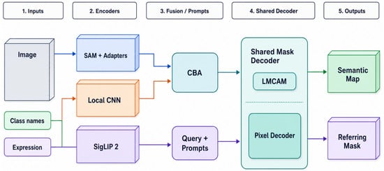
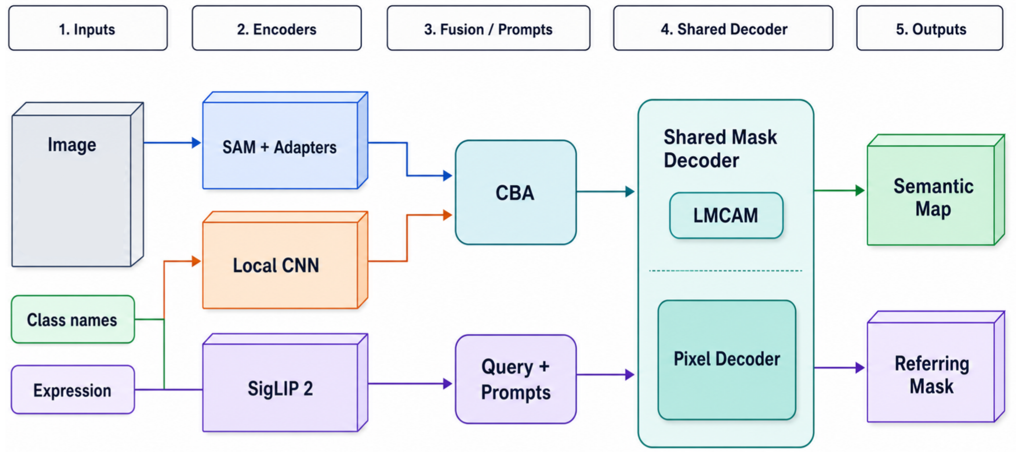
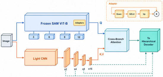
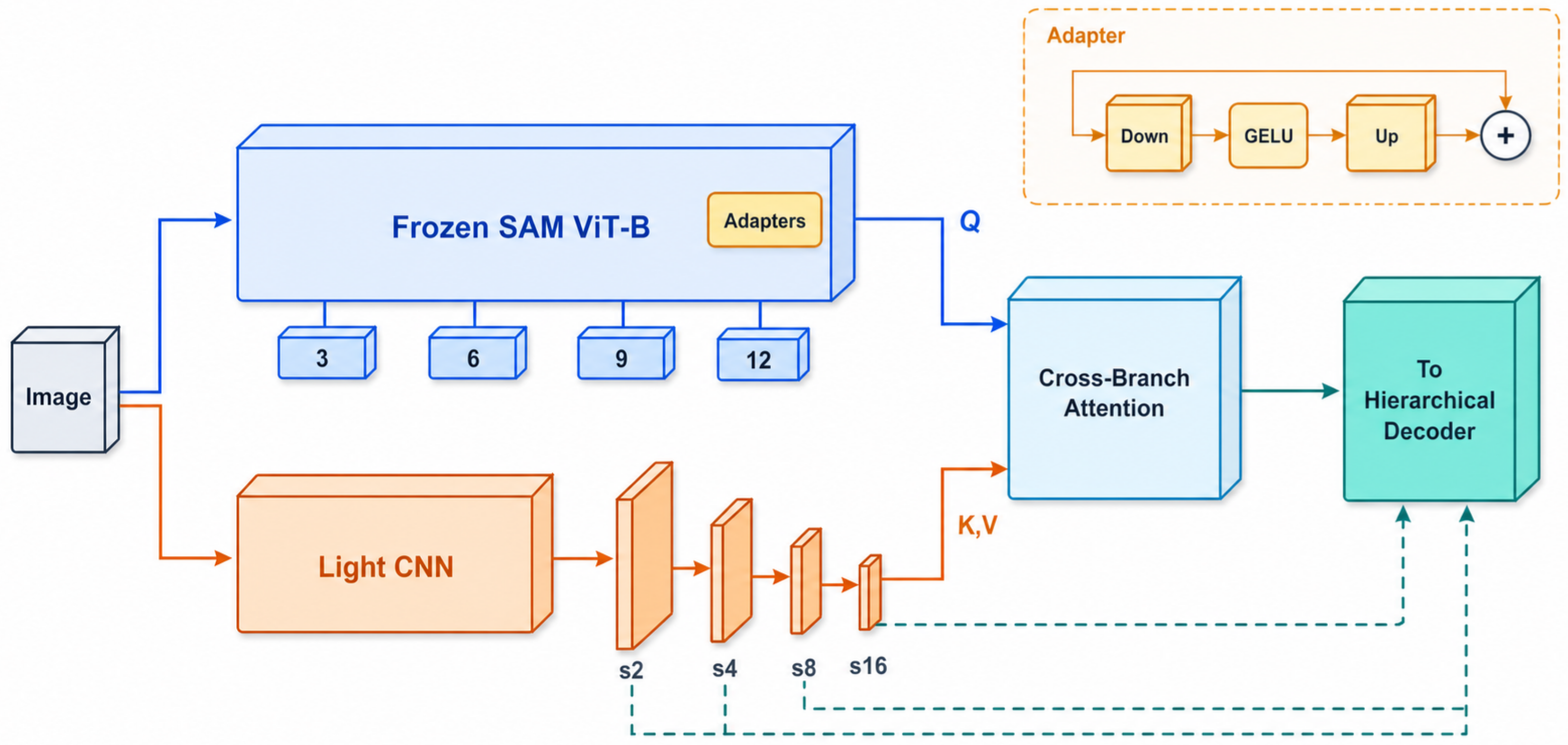
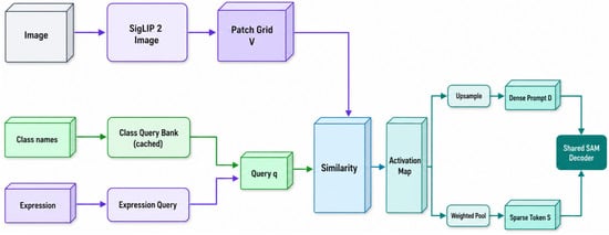
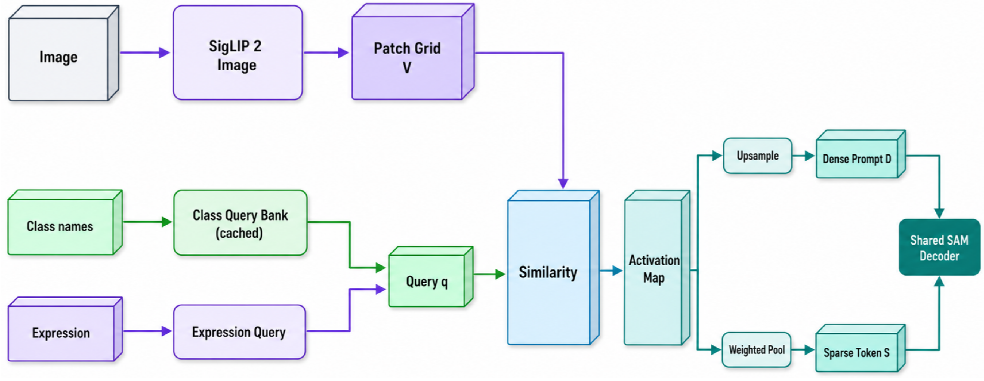
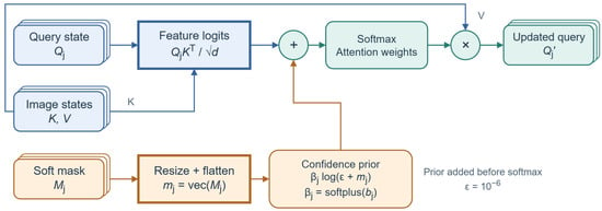
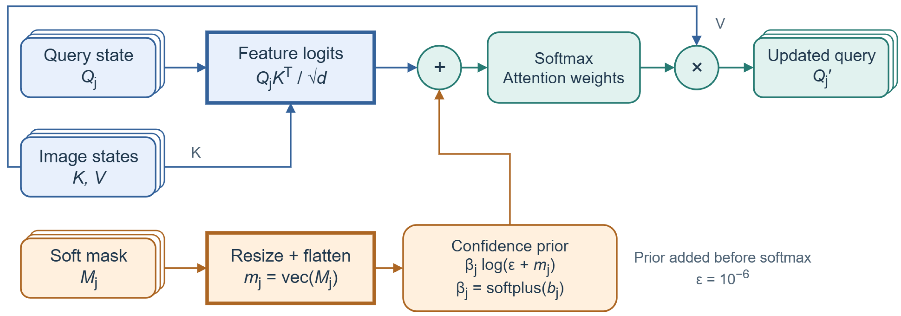
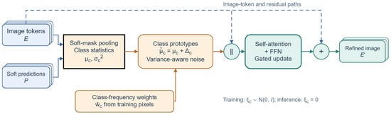
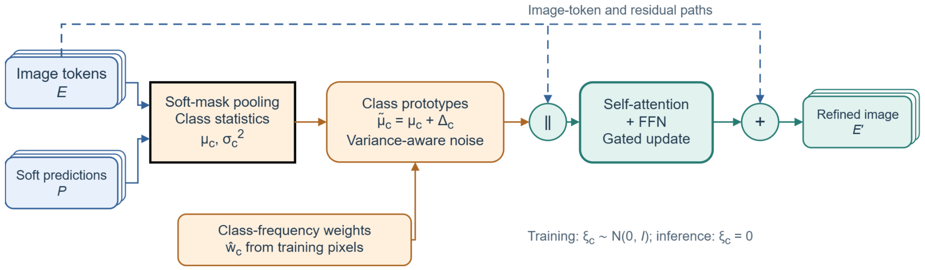
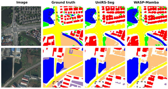
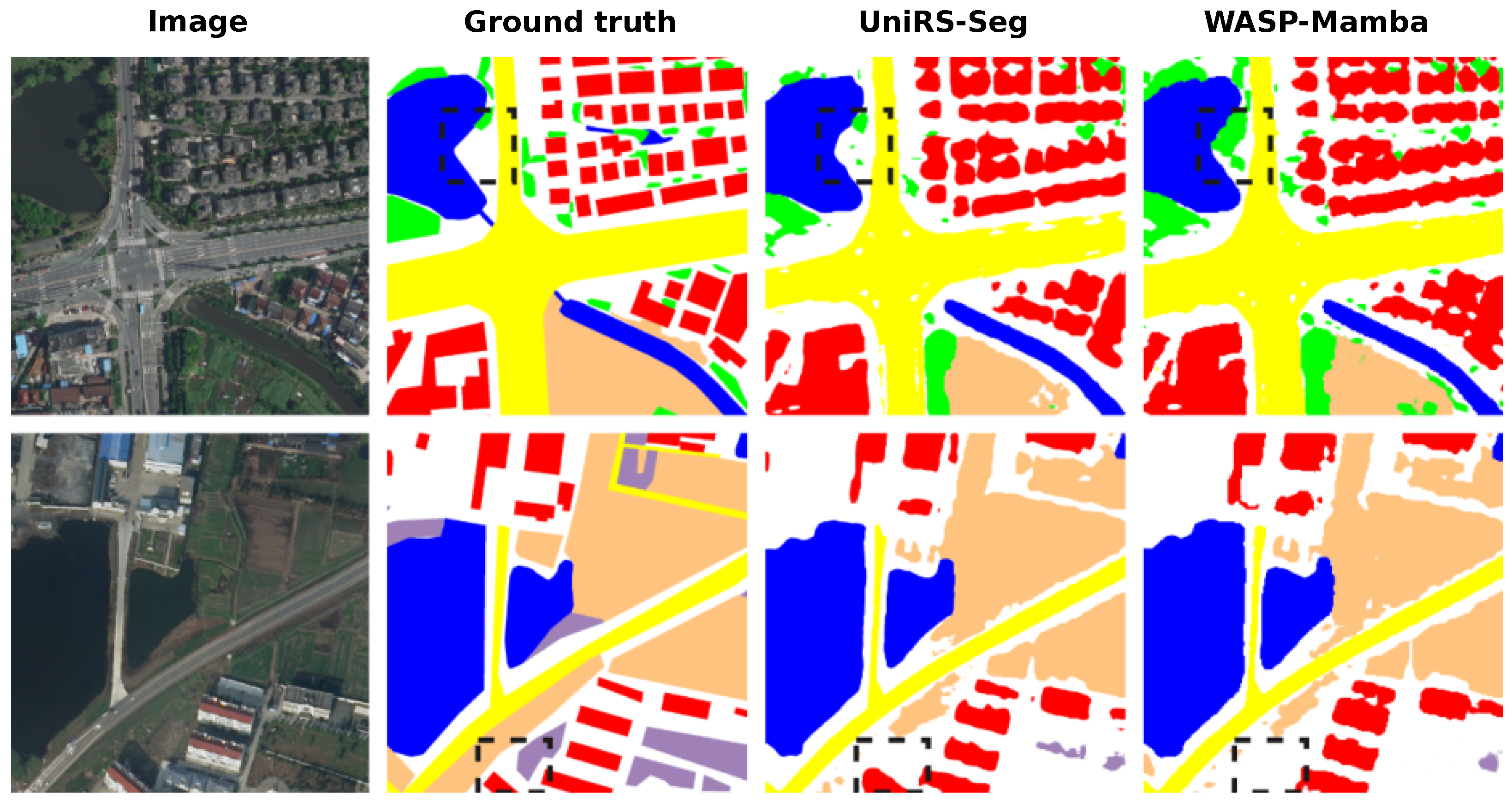
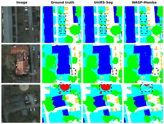
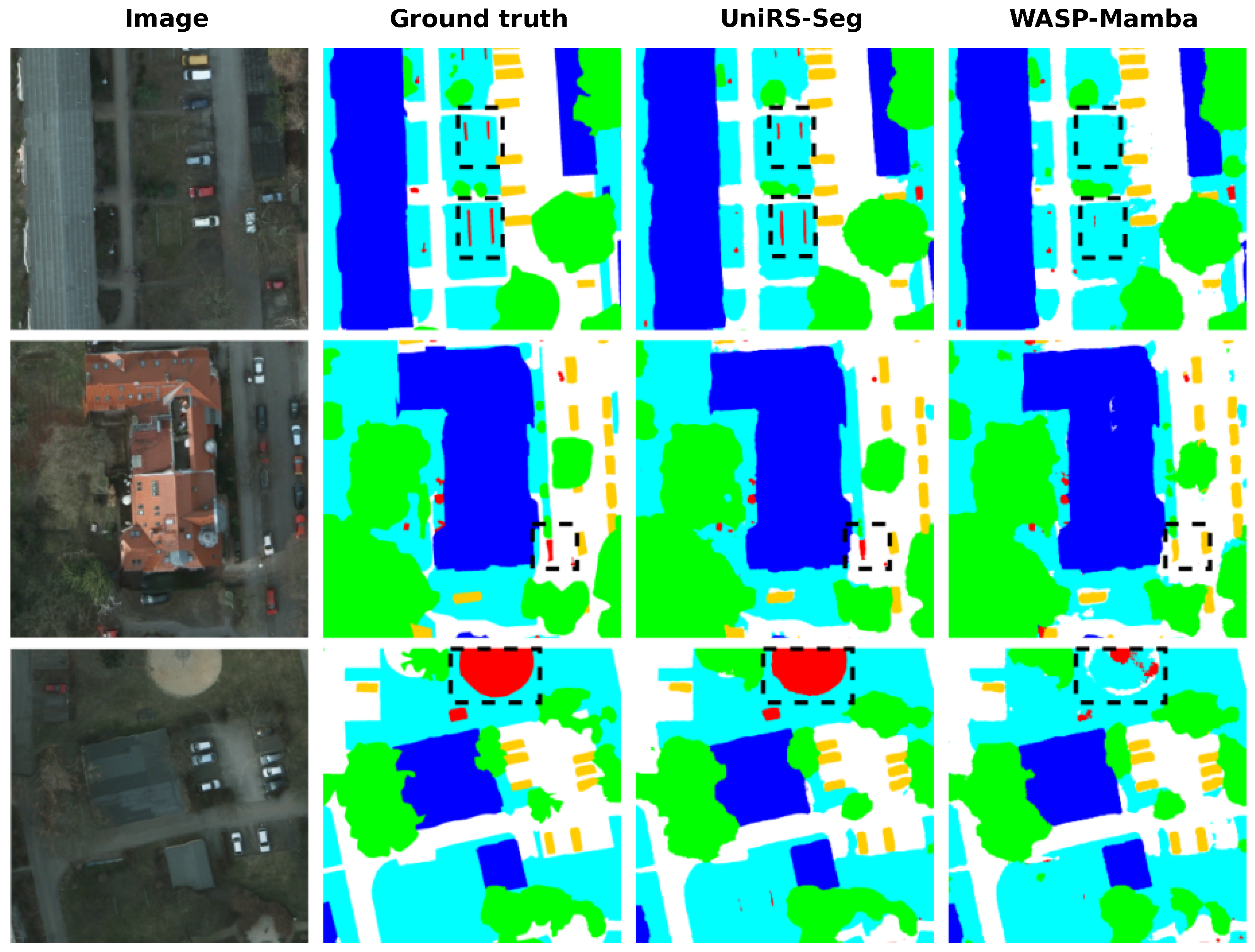
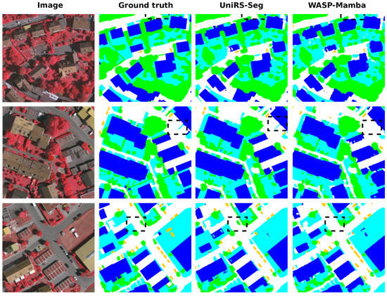
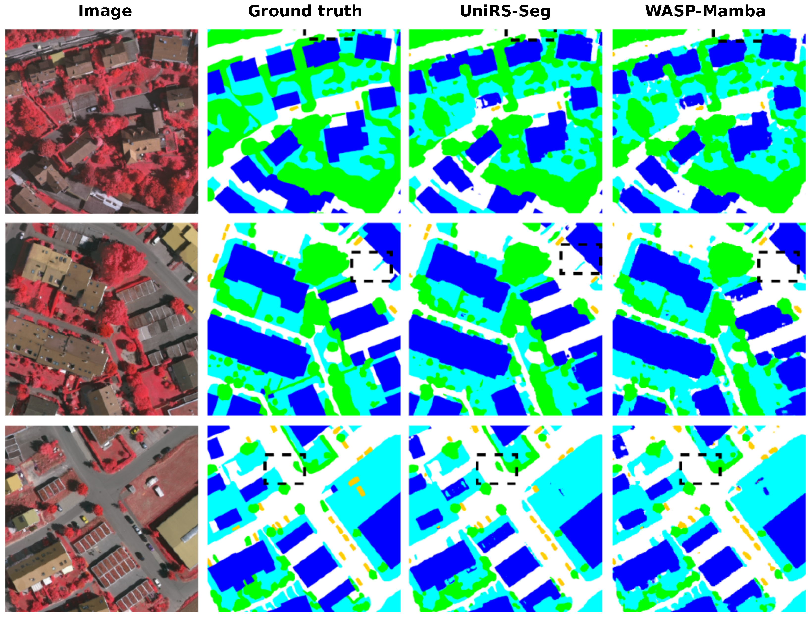
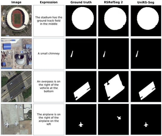
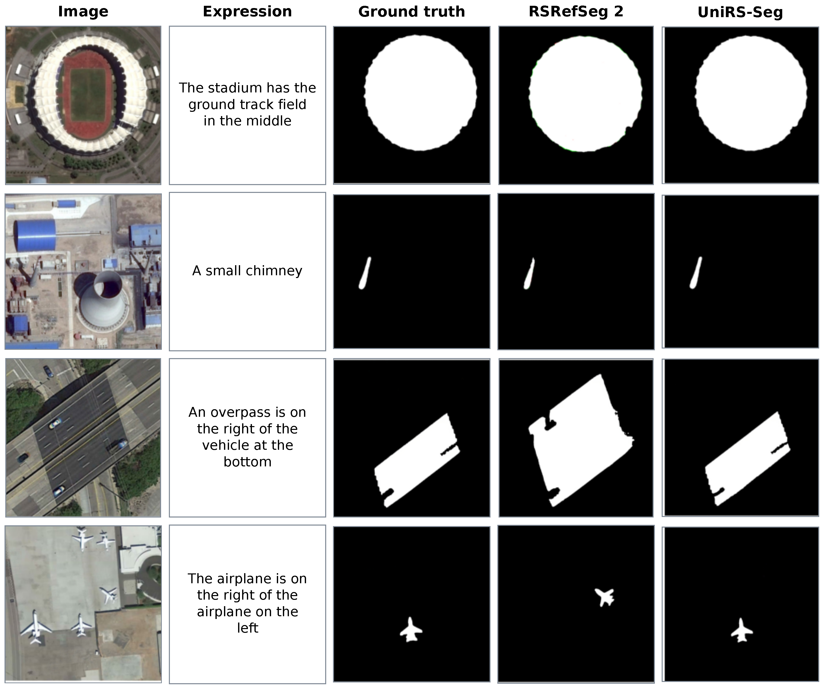
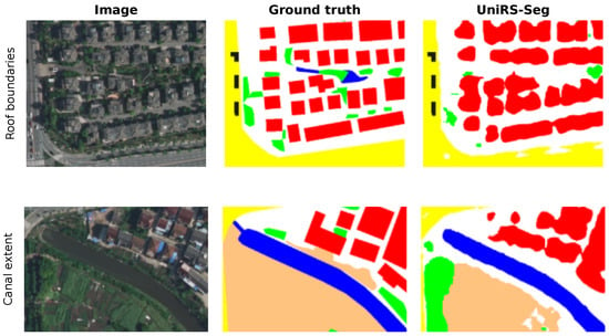
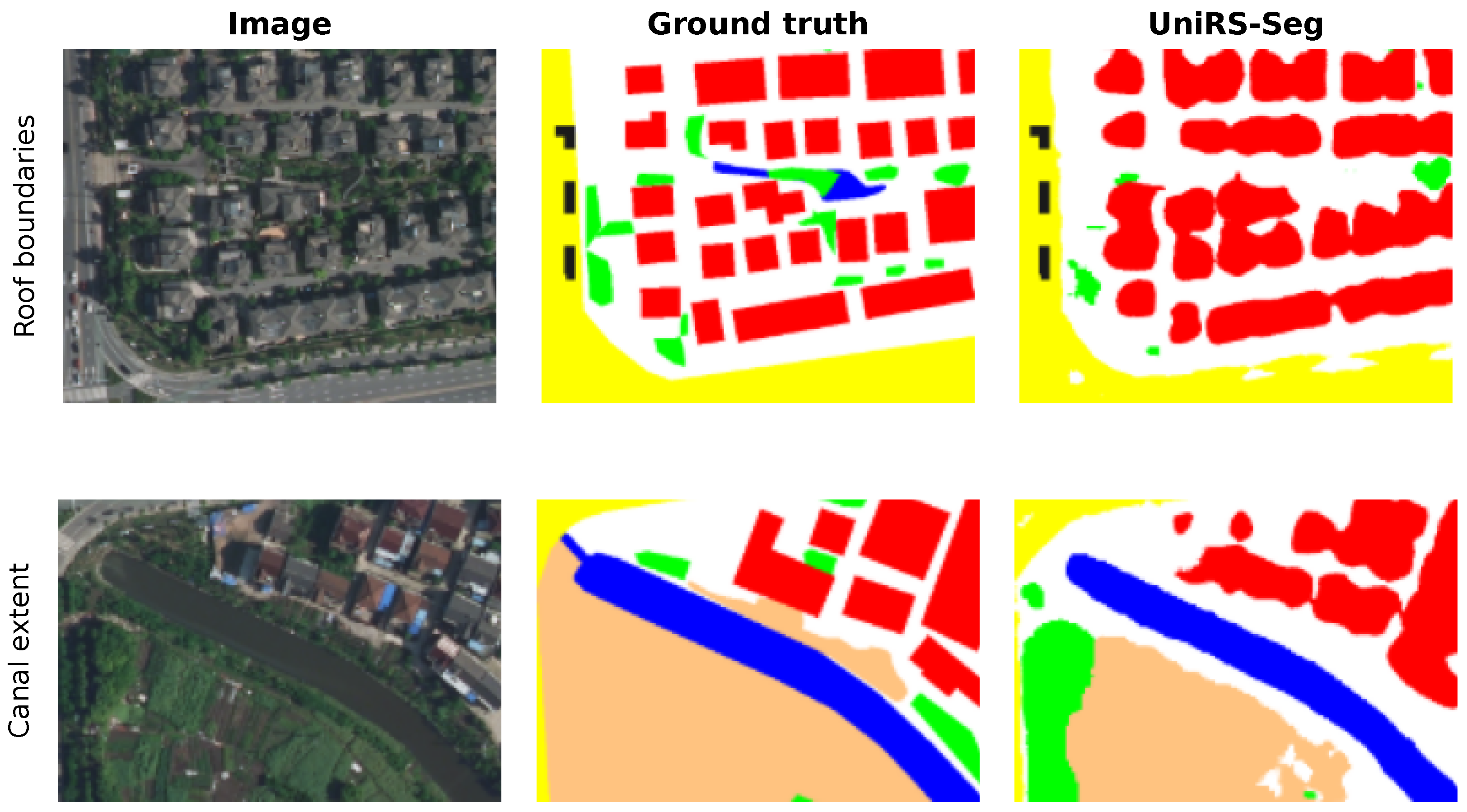

Disclaimer/Publisher’s Note: The statements, opinions and data contained in all publications are solely those of the individual author(s) and contributor(s) and not of MDPI and/or the editor(s). MDPI and/or the editor(s) disclaim responsibility for any injury to people or property resulting from any ideas, methods, instructions or products referred to in the content. |
© 2026 by the authors. Licensee MDPI, Basel, Switzerland. This article is an open access article distributed under the terms and conditions of the Creative Commons Attribution (CC BY) license.